Frustrated magnets in the limit of infinite dimensions: dynamics and disorder-free glass transition

Abstract

We study the statistical mechanics and the equilibrium dynamics of a system of classical Heisenberg spins with frustrated interactions on a $d$-dimensional simple hypercubic lattice, in the limit of infinite dimensionality $d\to\infty$. In the analysis we consider a class of models in which the matrix of exchange constants is a linear combination of powers of the adjacency matrix. This choice leads to a special property: the Fourier transform of the exchange coupling $J(\mathbf{k})$ presents a $(d-1)$-dimensional surface of degenerate maxima in momentum space. Using the cavity method, we find that the statistical mechanics of the system presents for $d\to\infty$ a paramagnetic solution which remains locally stable at all temperatures down to $T=0$. To investigate whether the system undergoes a glass transition we study its dynamical properties assuming a purely dissipative Langevin equation, and mapping the system to an effective single-spin problem subject to a colored Gaussian noise. The conditions under which a glass transition occurs are discussed including the possibility of a local anisotropy and a simple type of anisotropic exchange. The general results are applied explicitly to a simple model, equivalent to the isotropic Heisenberg antiferromagnet on the $d$-dimensional fcc lattice with first and second nearest-neighbour interactions tuned to the point $J_{1}=2J_{2}$. In this model, we find a dynamical glass transition at a temperature $T_{\rm g}$ separating a high-temperature liquid phase and a low temperature vitrified phase. At the dynamical transition, the Edwards-Anderson order parameter presents a jump demonstrating a first-order phase transition.

I Introduction

Many important phenomena in magnetism are controlled by frustration. Striking examples are spin systems on triangular, kagome, pyrochlore, fcc, and other geometrically-frustrated lattices, which present an extremely rich and complex phenomenology [1]. In many of these systems, frustration forces every plaquette to present multiple degenerate minima. In the lattice, when plaquettes share corners or edges, this leads often to striking collective behaviors.

At the same time, frustration is a key ingredient in systems displaying rugged energy landscapes, slow relaxation, and glassy dynamics. Prototype examples are spin glasses [2, 3], controlled by a random distribution of exchange couplings. However, frustration has a central role also in one of the theories for the vitrification of liquids [4, 5], in Coulomb-frustrated models [6, 4, 7, 8, 9, 10, 11, 12, 13, 14, 5] and in systems which present random patterns of stripes [15], relevant, for example, in Coulomb-frustrated charge separation [6], ferromagnetic thin films [16], and possibly even biology [17]. More precisely, we are talking about models with frustration induced by competition between short-range and long-range interactions, the latter can be Coulomb or dipole-dipole, or can have another nature. Here in the paper we will use the term “Coulomb-frustrated” to refer to such models, just for brevity. These models are closely connected to the phenomenon of avoided criticality [5]. In Coulomb-frustrated theories, complementary theoretical analyses [6, 4, 7, 8, 9, 10, 11, 12, 13, 14, 5] and numerical simulations [11] have given strong indications of the emergence of a glassy behavior even in absence of a quenched disorder. Similar behavior was shown to happen in magnetic systems with dipole-dipole interactions [15] and in Brazovskii-like models with a line of minima of exchange energy [18, 15].

A natural question is therefore: under which conditions frustration alone is sufficient to generate a glassy state? This question has been a subject of investigations for decades. Many theoretical models have been analyzed, for example fully-frustrated spin systems [19, 20, 21, 22], kinetically-constrained models [23], spin-systems with three-body interactions [24], and models of Josephson-junction arrrays [25, 26, 27].

In the context of geometrically frustrated magnets, the possibility of a glass transition in absence of disorder has attracted interest as an explanation to the behavior experimentally oberved in some kagome and pyrochlore materials [28, 29, 30]. The presence of disorder-free glassiness in these materials remains a subject of controversy.

Recently, systems which combine a geometrically frustrated lattice with a long-range interaction have attracted attention. In Ref. [31], it has been shown by numerical methods that an electron system with Coulomb repulsion on the triangular lattice undergoes an “electron glass” transition at quarter filling. The mechanism proposed for the emergence of glassiness is that the long-range force lifts the degeneracy between the many classical ground states on the triangular lattice, introducing large energy barriers and a rugged landscape. The disorder-free glass transition detected theoretically has been proposed as an explanation for the slow dynamics observed in an organic conductor [31].

Another theory analyzed recently which combines similarly a frustrated geometry and a long-range coupling is the Ising model with dipolar interaction on the kagome net. For this model, Ref. [32] found numerical evidence of a glass transition and a slow relaxation consistent with the Vogel-Fulcher law. The model has been analyzed in Ref. [33] by an analytical method, based on the Bethe-Peierls approximation. The results confirmed the existence of a glass transition, although the second-order transition found in Ref. [33] indicates a divergence of the relaxation time different from the Vogel-Fulcher law, and similar to that of disordered spin glasses.

On the experimental side, two recent works [34, 35] indicated that a disorder-free glass transition can occur even in an elemental solid: the rare earth neodymium (Nd). In particular, Refs. [34, 35] reported evidence of ageing, ultraslow dynamics, and a complex amorphous structures in nanoscale magnetization patterns imaged by spin-polarized scanning tunneling microscopy on the surface of Nd. It was shown that the randomness of the observed patterns becomes enhanced, and not reduced, when the defect concentration is lowered. This points to a theoretical explanation in terms of a “self-induced spin glass” (“self-induced” means an assumption that frustrations alone are sufficient for the spin-glass behavior in deterministic systems) [16, 15]. Refs. [34, 35] suggested, in particular. This scenario has been corroborated by the observation of slow relaxation in spin dynamics simulations, performed using exchange constants calculated from first principles.

The results found recently motivate us to investigate an exactly solvable spin model exhibiting a disorder-free glass transition. In particular, we revisit a model studied by Lopatin and Ioffe [36], which has as its key ingredient a frustrated antiferromagnetic on a large-dimensional hypercubic lattice. In the work of Ref. [36], the model was introduced as a lattice theory for the glass transition of supercooled liquids, and presented as fundamental degrees of freedom, a set of Ising spins representing particles ($S_{i}=+1$) and holes ($S_{i}=-1$). The interaction was constructed assuming a matrix of exchange couplings of the form $J_{ij}=[f(\hat{t}/\sqrt{2d})]_{ij}$ with $f(x)=-ux^{2}$ and $\hat{t}$ the adjacency matrix (a matrix $t_{ij}$ such that $t_{ij}=1$ if $i$ and $j$ are nearest neighbours and $t_{ij}=0$ otherwise). Ref. [36] solved the problem for an arbitrary chemical potential using a replica method. Despite the simplicitly of the model, it was shown that the system undergoes a dynamical and a static glass transition.

In this work, we study a similar model in the case in which the degrees of freedom are classical spin vectors $\mathbf{S}_{i}$. The continuous nature of the degrees of freedom allows us to study the possibility of a vitrification transition from a dynamical analysis. In the main part of the work, we derive a solution of the model, exact in the limit $d\to\infty$, including the possibility of anisotropy. Eventually, we apply the results to a special case: an isotropic model with $f(x)=J(x^{2}-1)$, $J<0$. After separation of the hypercubic lattice into sublattices, this model is equivalent to two decoupled Heisenberg models on the fcc structure. In particular, the model has two nonzero couplings: a nearest neighbour interaction of strength $J_{1}=J/d$ and a second-nearest-neighbour interaction of magnitude $J_{2}=J/(2d)$. For this model we identify a dynamical first-order glass transition, signaled by a jump of the Edwards-Anderson order parameter. The transition occurs even in absence of quenched disorder: the glass phase is self-induced.

The class of interactions $J_{ij}=[f(\hat{t}/\sqrt{2d})]_{ij}$ has a special property, which has not been emphasized in Ref. [36]: it implies that the Fourier transform $J(\mathbf{k})$ of the exchange coupling develops a $(d-1)$-dimensional surface of degenerate maxima in momentum space [37].

Similar surfaces appear in the Brazovskii model and with Coulomb-frustrated theories [6, 4, 7, 8, 9, 10, 11, 12, 13, 14, 5, 16, 15]. In Coulomb-frustrated models, the emergence of a glass phase has been investigated intensively using broken replica symmetry, with the specific tools borrowed from the theory of conventional, that is, disordered, spin glasses [38]. In particular, replica analyses based on the self-consistent screening approximation (SCSA) [8] and on local mean-field approximations [10, 14] predicted a glassy behavior of the random first-order type. The presence of a dynamical arrest has been confirmed by numerical simulations, and by an analytical study based on a mode-coupling theory and a dynamic SCSA [11, 12]. In dipole-frustrated [15] and for Brazovskii-like models [14, 15] analogue glass transitions have been shown by replica methods.

In Coulomb-frustrated models the surface of maxima occurs usually in the region of small momenta, at characteristic wavelengths much larger than the atomic spacing. In addition, the interactions have an infinite range. These factors introduce differences with respect to the model studied here, where the interactions are short-ranged and the degenerate surface lies in a region of large wavevectors, comparable with the size of the Brillouin zone. Despite these differences the analogy remains close. Thus we can consider the model as an exactly solvable theory exemplifying the “stripe glass” behavior, at a dynamical mean-field level. The methology used in our work allows to study vitrification in a physically transparent approach, based on explicit consideration of spin dynamics at large time scale, in analogy with the pioneering work by Edwards and Anderson on spin glasses [2] and to the mode coupling approach by Götze in the theory of structural glasses [39].

The range of applications of the model is even broader. The theory analyzed here allows to investigate, in infinite dimensions, the model of a frustrated magnet with a degenerate surface of helical states. Spin systems with degenerate manifolds of spiral ground states space have attracted an extensive interest and have been predicted to host spiral spin liquid phases (see Refs. [40, 37, 41, 42] for theoretical analyses and for experimental evidences of spiral spin liquid states in cubic spinels).

The article is organized as follows. In Sec. II, we introduce the model analyzed in this work. In Sec. III, we derive an exact solution of the equilibrium statistical mechanics of the system in the limit $d\to\infty$. The solution shows that renormalizations stabilize the paramagnetic solution at all temperatures down to $T=0$, a situation analogue to the “avoided criticality” [7]. In Sec. IV, we study the dynamics of the system, assuming a purely dissipative Langevin equation. In the large-$d$ limit, we show that the problem maps to an effective single-site Langevin equation with a colored noise, self-consistently determined by a set of consistency relations. The conditions under which the dynamics develops a glass transition are discussed in Sec. V. The general results are applied explicitly in the case of a isotropic Heisenberg model, and for a simple interaction $J_{ij}=[f(\hat{t}/\sqrt{2d})]_{ij}$ with $f(x)=J(x^{2}-1)$. The results for this minimal model are presented in Sec. VI. We conclude the article with a brief summary in Sec. VII.

II Model

Although we eventually focus on isotropic models, in the main part of the work we keep the discussion more general, and analyze spin systems subject to both an exchange interaction $J_{ij}^{\alpha\beta}$ and an on-site anisotropy $V(\mathbf{S}_{i})$. We thus assume a Hamiltonian:

$$H=-\frac{1}{2}\sum_{i,j}J^{\alpha\beta}_{ij}S^{\alpha}_{i}S^{\beta}_{j}+\sum_{i}V(\mathbf{S}_{i})~{}.$$ (1)

The degrees of freedom $\mathbf{S}_{i}$ are classical spins: three-dimensional vectors with cartesian coordinates $S^{\alpha}_{i}$, $\alpha=x,y,z$ and with the constraint of unit length $\mathbf{S}^{2}_{i}=S^{\alpha}_{i}S^{\alpha}_{i}=1$. The labels $i$, $j$ run over the sites of a hypercubic lattice in $d$ dimensions. In the analysis we take eventually the limit of large dimensionality $d\to\infty$. The $d\to\infty$ approximation [43] has demonstrated its power for the consideration of lattice fermionic problems where it is the base of dynamical mean-field theory (DMFT), for reviews see Refs. [44, 45, 46].

The anisotropy energy $V(\mathbf{S}_{i})$ in the model may be arbitrary. We make the only assumption that it is even ($V(\mathbf{S}_{i})=V(-\mathbf{S}_{i})$) in such way that $H$ is invariant under time-reversal, that is, spin-reversal.

The main ingredient in the model, controlling the frustration and the emergence of glassiness, is a strongly frustrated exchange coupling $J^{\alpha\beta}_{ij}$. Here we consider a coupling of the form $J_{ij}^{\alpha\beta}=[f^{\alpha\beta}(\hat{t}/\sqrt{2d})]$, where $f^{\alpha\beta}(x)$ a $3\times 3$ matrix of functions and the factor $1/\sqrt{2d}$ is introduced to have a well-defined large-$d$ limit [36, 47]. This interaction is a simple generalization of the coupling considered by Lopatin and Ioffe [36]. In the definition $f(x)$ is assumed to be a polynomial and powers of $\hat{t}$ are intended in the sense of matrix multiplication. For example, the function $f^{\alpha\beta}(x)=J_{0}^{\alpha\beta}+J_{1}^{\alpha\beta}x+J_{2}^{\alpha\beta}x^{2}+J_{4}^{\alpha\beta}x^{4}$ describes the coupling

$$\begin{split}J_{ij}^{\alpha\beta}&=J_{0}^{\alpha\beta}\delta_{ij}+\frac{J_{1}^{\alpha\beta}}{\sqrt{2d}}t_{ij}+\frac{J_{2}^{\alpha\beta}}{2d}\sum_{k}t_{ik}t_{kj}\\ &+\frac{J_{4}^{\alpha\beta}}{4d^{2}}\sum_{k,l,m}t_{ik}t_{kl}t_{lm}t_{mj}~{}.\end{split}$$ (2)

The matrix elements $[\hat{t}^{n}]_{ij}$ are equal to the number of paths which start at $i$, end at $j$, and are constituted by a sequence of $n$ steps along the bonds of the hypercubic lattice. In particular, $[\hat{t}^{n}]_{ij}$ is zero if the Manhattan distance $\ell_{ij}$ between $i$ and $j$ is greater than $n$. Thus the interaction is short ranged: if $f^{\alpha\beta}(x)$ is a polynomial of degree $R$, the exchange couplings are nonzero only up to a maximum range equal to $R$.

For convenience, we assume that the on-site exchange $J_{ii}^{\alpha\beta}=0$ (this does not imply a loss of generality because any local interaction can be absorbed in a redefinition of $V(\mathbf{S}_{i})$). This requires to choose a constant term $j_{0}^{\alpha\beta}$ in such way to cancel the contributions of the on-site matrix elements $[\hat{t}^{2}]_{ii}$, $[\hat{t}^{4}]_{ii}$, $[\hat{t}^{6}]_{ii}$, … In the limit of large dimensionality: $[\hat{t}^{2n}]_{ii}$ is of order $d^{n}$ [25]. Thus $[(\hat{t}/\sqrt{2d})^{2n}]$ is finite for $d\to\infty$. In particular we can choose a finite $j_{0}^{\alpha\beta}$ to impose the condition $J_{ii}^{\alpha\beta}=0$.

As it was anticipated in Sec. I, the exchange coupling $J^{\alpha\beta}_{ij}$ generates, under some conditions, a surface of maxima in momentum space. This follows from the fact that the Fourier transform of the interaction is

$$J^{\alpha\beta}(\mathbf{k})=\sum_{i}{\rm e}^{-i\mathbf{k}\cdot(\mathbf{x}_{i}-\mathbf{x}_{j})}J^{\alpha\beta}_{ij}=f^{\alpha\beta}(\varepsilon_{\mathbf{k}})~{},$$ (3)

with $\varepsilon_{\mathbf{k}}=\sqrt{2/d}\sum_{a=1}^{d}\cos(k_{a})$. Thus $J^{\alpha\beta}(\mathbf{k})$ depends on the wavevector $\mathbf{k}$ only through $\varepsilon_{\mathbf{k}}$. The variable $\varepsilon_{\mathbf{k}}$ is restricted to $-\sqrt{2d}<\varepsilon_{\mathbf{k}}<\sqrt{2d}$, but for $d\to\infty$ the bounds diverge and the variable $\varepsilon_{\mathbf{k}}$ takes values on the entire real axis. If the eigenvalues of $f^{\alpha\beta}(\varepsilon)$ are bounded from above on the real axis $-\infty<\varepsilon<\infty$, then the maximum eigenvalues of $J^{\alpha\beta}(\mathbf{k})$ occur on a $(d-1)$-dimensional surface: the manifold satisfying $\varepsilon_{\mathbf{k}}=\varepsilon_{\rm max}$ (with $\varepsilon_{\rm max}$ the point, or points, at which $f^{\alpha\beta}(\varepsilon)$ reaches its maximum eigenvalue).

To get a first understanding of the frustration in the model, it is useful to discuss its statistical mechanics at the level of a Weiss mean-field theory (MFT). Consider for simplicity the case of a isotropic model, with $V(\mathbf{S})=0$, and $f^{\alpha\beta}(\varepsilon)=\delta^{\alpha\beta}f(\varepsilon)$, and assume that $f(\varepsilon)=J(\varepsilon^{2}-1)$. It is simple to check that the constant term $-1$ in the definition of $f(\varepsilon)$ ensures $J_{ii}=0$, since $[(\hat{t}/\sqrt{2d})^{2n}]=1$. Within MFT, the susceptibility in the paramagnetic phase is given by

$$\chi^{-1\alpha\beta}(\mathbf{k})=\chi_{0}^{-1\alpha\beta}-J^{\alpha\beta}(\mathbf{k})~{},$$ (4)

where $\chi_{0}^{\alpha\beta}=\delta^{\alpha\beta}/(3k_{\rm B}T)$ is the susceptibility of single spin (in the isotropic case). The theory, therefore, predicts a second-order transition at a critical temperature $T_{\rm MFT}=J_{\rm max}/(3k_{\rm B})$ where $J_{\rm max}$ is the maximum value of $J(\mathbf{k})$. By Eq. (3), $J_{\rm max}$ simply equal to the maximum $f_{\rm max}$ of the function $f(x)$. If the coupling is ferromagnetic ($J>0$), $f(\varepsilon)$ is not bounded from above. In this case the interaction is not frustrated and the large-$d$ limit is unstable. A well-defined $d\to\infty$ theory would require to scale the interaction differently [47] (assigning to the adjacency matrix a scaling factor $1/d$ instead of $1/\sqrt{2d}$). If instead $J<0$, $J_{\rm max}=f_{\rm max}=|J|$. The Weiss transition temperature is, therefore, $T_{\rm MFT}=|J|/(3k_{\rm B})$.

The fact that $T_{\rm MFT}$ remains finite for $d\to\infty$ signals the very strong frustration of the problem. In fact, the model presents an interaction of range $2$ and magnitude of order $J/d$. The coordination number, however, grows as $z\approx d^{2}$ for $d$ large. Thus, if the interactions were not strongly frustrated, we would expect a critical temperature which diverges for $d\to\infty$ as $z|J_{2}|d^{-1}\approx d^{2}\times d^{-1}\propto d$. The fact that this divergence does not occur shows that the interactions are in strong mutual competition. In particular, the finiteness of the limit $d\to\infty$ shows that the situation is similar to other frustrated models with large coordination numbers: the local fields $\sum_{j}J_{ij}\mathbf{S}_{j}$ which act on a site $i$ do not scale linearly with the dimension $d$ but only as their square root $\sqrt{d}$ [20].

The presence of an infinitely strong frustration can also be understood by calculating the energy of the helical ground states of the system. The system admits spiral ground states of the form: $\mathbf{S}_{i}=\mathbf{A}_{i}\cos(\mathbf{k}\cdot\mathbf{x}_{i})+\mathbf{B}_{i}\sin(\mathbf{k}\cdot\mathbf{x}_{i})$, with $\mathbf{A}_{i}^{2}=\mathbf{B}_{i}^{2}=1$, $(\mathbf{A}_{i}\cdot\mathbf{B}_{i})=0$ [7, 37, 41], and $\mathbf{k}$ any wavevector which maximizes $J(\mathbf{k})$. For the antiferromagnetic interaction $f(\varepsilon)=J(\varepsilon^{2}-1)$, $J<0$, the set of $\mathbf{k}$-points maximizing $J(\mathbf{k})$ is the $(d-1)-$dimensional surface $\varepsilon_{\mathbf{k}}=\sum_{a=1}^{d}\cos(k_{a})=0$. There is therefore a degenerate manifold of helical ground states. The energy per particle in any of these plane-wave states is: $E/N=-f_{\rm max}/2=-|J|/2$. This shows again an extremely strong frustration. In fact any site interacts with $z\approx 2d^{2}$ neighbours via a coupling of magnitude $|J|/d$. If the spins could be lined up in such way to extract a finite fraction of the available energy $|J|/d\times z=|J|/d\times 2d^{2}$, then the ground state energy would diverge. However due to frustration, only a fraction $\approx 1/\sqrt{d}$ of the energy can be extracted, and thus $E/N$ remains finite.

The same considerations apply for any $f(\varepsilon)$. If $f(\varepsilon)$ is not bounded from above, the large-$d$ limit is unstable and the MFT transition temperature diverges. This case corresponds to non-frustrated or weakly-frustrated models, which we do not analyze in this work. If instead $f(\varepsilon)$ is bounded from above, the interaction is strongly frustrated, and the large-$d$ limit is stable, as indicated by a finite $T_{\rm MFT}$. The finiteness of $T_{\rm MFT}$ at the level of mean field theory is again a sign of a very strong frustration. In fact, the expansion of $J_{ij}^{\alpha\beta}=[f^{\alpha\beta}(\hat{t}/\sqrt{2d})]_{ij}$ generates a coupling $J_{ij}^{\alpha\beta}$ of order $d^{-\ell_{ij}/2}$ where $\ell_{ij}$ is the Manhattan distance between $i$ and $j$. The suppression factor $d^{-\ell_{ij}/2}$ does not compensate the growth of the coordination numbers $z_{\ell}\propto d^{\ell}$. Thus, in absence of frustration, we would expect a divergence $T_{\rm MFT}\approx z_{R}|J_{R}|d^{-R/2}\propto d^{R}\times d^{-R/2}\approx d^{R/2}$, where $R$ is the maximum range of the interaction.

In anisotropic models, the criterion for frustration and stability of the $d\to\infty$ limit are analogue. In order for the $d\to\infty$ to be finite, all eigenvalues of $f^{\alpha\beta}(\varepsilon)$ must be bounded from above on the real axis $-\infty<\varepsilon<\infty$. Throughout this work, we assume everywhere this condition is satisfied [48].

The conditions under which $f$, or its eigenvalues, are bounded has a simple geometrical interpretation. Suppose that the interaction has a range $R$, and, thus, that $f^{\alpha\beta}(\varepsilon)=\sum_{m=0}^{R}J_{m}^{\alpha\beta}\varepsilon^{m}$ is a polynomial of degree $R$. If the maximum degree $R$ is odd, it is clear that the eigenvalues cannot be bounded: depending on the signs of $J_{R}^{\alpha\beta}$, the system presents ferromagnetic or antiferromagnetic instabilities. Thus $R$ must be even. In addition, the interaction of maximum range $J^{\alpha\beta}_{R}$ must be antiferromagnetic [49]. The hypercubic lattice in $d$ dimensions is bipartite and can be viewed as composed of two interpenetrating sublattices: the sublattice A composed of the sites such that the sum $\sum_{a=1}^{d}x_{a}$ of the coordinates $(x_{1},....,x_{d})$ is an even integer and the complementary sublattice B where the sum $\sum_{a=1}^{d}x_{a}$ is an odd integer. The structure of A and B is that of a generalized $d$-dimensional fcc lattice [50]. Interactions with even range couple the spins within the same sublattice ($A-A$ or $B-B$), while interactions with an odd range induce a coupling between different sublattices ($A-B$ and $B-A$).

Thus, in infinite dimensions and within the class ofinteractions $J_{ij}^{\alpha\beta}=[f^{\alpha\beta}(\hat{t}/\sqrt{2d})]_{ij}$, frustration requires that the coupling of longest range is antiferromagnetic and takes place within the fcc sublattices. It is well known that the fcc geometry is frustrated [21, 50, 37].

In Sec. VI, we consider explicitly the isotropic model with $f(\varepsilon)=J(\varepsilon^{2}-1)$, $J<0$. In this model—and in any case in which $f(\varepsilon)$ is an even function—the two fcc sublattices are decoupled. Thus the system breaks into two independent copies of a frustrated model on the fcc structure. The reduced fcc model has a nearest-neighbour interaction $J_{1}=J/d$ and a second-nearest-neighbour interaction $J_{2}=J/(2d)$. The presence of the $J_{2}$ coupling makes the model different from the fully-frustrated fcc antiferromagnet [21], in which only nearest-neighbour interaction are present. Instead, the model extends, to infinite dimensions, the problem of an $J_{1}=2J_{2}$ fcc antiferromagnet. As in three dimensions [37], the $J_{1}=2J_{2}$ antiferromagnet presents a degenerate manifold of helical modes, which is absent in the nearest-neighbour fcc model.

Notations.—Throughout the paper we will use the following notations. The symbol $\int_{\mathbf{S}_{i}}$ stands for an integral over all values of the spin $\mathbf{S}_{i}$ (in spherical coordinates $\int_{\mathbf{S}_{i}}=\int_{0}^{\pi}\sin\theta_{i}{\rm d}\theta_{i}\int_{0}^{2\pi}{\rm d}\varphi_{i}$). $\delta_{S}(\mathbf{S}-\mathbf{S}^{\prime})$ is a delta function in spin space, defined according to the invariant measure (in spherical coordinates $\delta_{S}(\mathbf{S}-\mathbf{S}^{\prime})=\delta(\theta-\theta^{\prime})\delta(\varphi-\varphi^{\prime})/\sin\theta$). $3\times 3$ matrices such as $f^{\alpha\beta}(x)$ or $\chi^{\alpha\beta}$ are written in matrix notation with a symbol $\underline{\underline{f}}(x)$, $\underline{\underline{\chi}}$, etc. Matrices with lattice indices, such as $t_{ij}$ and $J_{ij}^{\alpha\beta}$, are denoted as $\hat{t}$, $\hat{J}$. Matrix multiplications and inverses are defined assuming contraction of all internal indices ($[\hat{A}\hat{B}]^{\alpha\beta}_{ij}=\sum_{k}A^{\alpha\gamma}_{ik}B^{\gamma\beta}_{kj}$, $[\hat{A}^{-1}\hat{A}]_{ij}^{\alpha\beta}=\sum_{k}A^{-1}{}^{\alpha\gamma}_{ik}A^{\gamma\beta}_{kj}=[\hat{1}]^{\alpha\beta}_{ij}=\delta^{\alpha\beta}\delta_{ij}$ for matrices with both spin and lattice indices; $[AB]_{ij}=\sum_{k}A_{ik}B_{kj}$ for matrices in site space only.)

III Static properties

In this section, we derive the solution, exact for $d\to\infty$, of the statistical mechanics of the system. As we show below, the result differs from the behavior indicated by the Weiss mean field theory. The system presents a paramagnetic state, with unbroken translation and spin inversion symmetries, which remains locally stable at all temperatures down to $T=0$. The stabilization of the paramagnetic phase occurs via a mechanism analogue to that which occurs in the Brazovskii model [18], and in Coulomb-frustrated systems [7]. The second-order magnetic instabilities are removed by strong renormalization effects, boosted by the presence of many low-lying modes near the degenerate surface.

To derive the solution, we use an approach based on the cavity method (in the context of DMFT for fermions, see Ref.47). As a starting point, we use a methodology analogue to the cavity approach applied in Ref. [3] to the Sherrington-Kirkpatrick (SK) spin-glass model. A key idea of this approach consists in analyzing the joint probability $P(\mathbf{S}_{i},\mathbf{b}_{i})$ of the spin $\mathbf{S}_{i}$ and the internal field $b^{\alpha}_{i}=\sum_{j}J^{\alpha\beta}_{ij}S^{\beta}_{j}$ at a single site $i$. In equilibrium at temperature $T$ [51]:

$$\begin{split}P(\mathbf{S}_{i},\mathbf{b}_{i})&=Z^{-1}\int_{\bar{\mathbf{S}}_{i_{1}}}..\int_{\bar{\mathbf{S}}_{i_{N}}}\big{[}\delta_{S}(\mathbf{S}_{i}-\bar{\mathbf{S}}_{i})\delta(\mathbf{b}_{i}-\bar{\mathbf{b}}_{i})\\ &\times{\rm e}^{-\beta H(\bar{\mathbf{S}}_{i_{1}},..\bar{\mathbf{S}}_{i_{N}})}\big{]}~{},\end{split}$$ (5)

where $Z$ is the partition function, $\beta=1/(k_{\rm B}T)$, $\bar{b}_{i}{}^{\alpha}=\sum_{j}J^{\alpha\beta}_{ij}\bar{S}_{j}{}^{\beta}$, and the integral is over all possible configurations of the $N$ spins. $P(\mathbf{S}_{i},\mathbf{b}_{i})$ can be interpreted, simply, as the probability that, extracting a random configuration at temperature $T$, the spin and the field at site $i$ have given values $\mathbf{S}_{i}$ and $\mathbf{b}_{i}$.

The reason why $P$ provides a particularly convenient framework for the analysis is that it describes efficiently a property of the large-$d$ limit: for $d\to\infty$ the field $\mathbf{b}_{i}$ has strong correlations with the spin $\mathbf{S}_{i}$ at the same site, but weaker correlations with the spins $\mathbf{S}_{j}$ at the other sites $j\neq i$. The consideration of a joint distribution allows to isolate the strong correlation of $\mathbf{b}_{i}$ with $\mathbf{S}_{i}$ factorizing

$$P(\mathbf{S}_{i},\mathbf{b}_{i})=Z^{\prime}_{i}Z^{-1}{\rm e}^{\beta(\mathbf{b}_{i}\cdot\mathbf{S}_{i})-\beta V(\mathbf{S}_{i})}p^{\prime}(\mathbf{b}_{i})~{}.$$ (6)

Here $Z^{\prime}_{i}$ and $p^{\prime}(\mathbf{b}_{i})$ are, respectively, the partition function and the distribution of the field $\mathbf{b}_{i}$ in a cavity system in which the site $i$ is removed. Explicitly,

$$Z^{\prime}_{i}=\int_{\mathbf{S}_{i_{2}}}...\int_{\mathbf{S}_{i_{N}}}{\rm e}^{-\beta H^{\prime}_{i}(\mathbf{S}_{i_{1}},...,\mathbf{S}_{i_{N}})}~{},$$ (7)

and

$$\begin{split}p^{\prime}(\mathbf{b}_{i})&=Z^{\prime}_{i}{}^{-1}\int_{\mathbf{S}_{i_{2}}}...\int_{\mathbf{S}_{i_{N}}}\big{[}\delta(b^{\alpha}_{i}-{\textstyle\sum}_{j}J^{\alpha\beta}_{ij}S^{\beta}_{j})\\ &\times{\rm e}^{-\beta H^{\prime}_{i}(\mathbf{S}_{i_{1}},...,\mathbf{S}_{i_{N}})}\big{]}~{},\end{split}$$ (8)

with

$$H^{\prime}_{i}=-\frac{1}{2}\sum_{j\neq i,k\neq i}J^{\alpha\beta}_{jk}S^{\alpha}_{j}S^{\beta}_{k}+\sum_{j\neq i}V(\mathbf{S}_{j})$$ (9)

the Hamiltonian of the cavity system (the $(N-1)$-particle system with the site $i$ removed). After the correlation with $\mathbf{S}_{i}$ is subtracted, the field distribution $p^{\prime}(\mathbf{b}_{i})$ has very simple statistical properties. In the limit $d\to\infty$, $p^{\prime}(\mathbf{b}_{i})$ becomes Gaussian:

$$p^{\prime}(\mathbf{b}_{i})=\frac{\exp\big{[}-L^{-1\alpha\beta}b^{\alpha}_{i}b^{\beta}_{i}/2\big{]}}{\sqrt{(2\pi)^{3}\det\underline{\underline{L}}}}$$ (10)

To prove this crucial fact we cannot use directly the methodology which applies to the SK model [3]. The reason is that in the SK model the nonlocal correlations $\mathopen{\hbox{${\langle}$}\kern-1.94444pt\leavevmode\hbox{${\langle}$}}S_{j}S_{k}S_{l}...\mathclose{\hbox{${\rangle}$}\kern-1.94444pt\leavevmode\hbox{${\rangle}$}}$ with $j\neq k\neq l\neq..$ give a negligible contribution to $p^{\prime}(\mathbf{b}_{i})$. In the model considered here, instead, the nonlocal parts $\langle S_{j}S_{k}\rangle$ contribute at leading order.

We thus use a perturbative approach, and analyze the cumulants of $p^{\prime}_{i}(\mathbf{b}_{i})$ within an expansion in powers of $J_{jk}$ (see Ref. [47] for a discussion of the cavity method in the context of DMFT). The $\ell$-th cumulant of $p^{\prime}(\mathbf{b}_{i})$ is equal to $C_{\ell}^{\prime}{}^{\alpha_{1}..\alpha_{\ell}}=\sum_{j_{1},j_{2},..j_{\ell}}J_{ij_{1}}^{\alpha_{1}\beta_{1}}...J_{ij_{\ell}}^{\alpha_{\ell}\beta_{\ell}}\mathopen{\hbox{${\langle}$}\kern-1.94444pt\leavevmode\hbox{${\langle}$}}S^{\beta_{2}}_{j_{2}}...S^{\beta_{\ell}}_{j_{\ell}}\mathclose{\hbox{${\rangle}$}\kern-1.94444pt\leavevmode\hbox{${\rangle}$}}^{\prime}{}^{(i)}$, where $\mathopen{\hbox{${\langle}$}\kern-1.94444pt\leavevmode\hbox{${\langle}$}}...\mathclose{\hbox{${\rangle}$}\kern-1.94444pt\leavevmode\hbox{${\rangle}$}}^{\prime}{}^{(i)}$ are connected averages computed in the cavity system (the symbol $\mathopen{\hbox{${\langle}$}\kern-1.94444pt\leavevmode\hbox{${\langle}$}}....\mathclose{\hbox{${\rangle}$}\kern-1.94444pt\leavevmode\hbox{${\rangle}$}}$ is used to denote connected averages, and the sign $\prime(i)$ reminds that the averaging is computed in a system with one cavity at site $i$). Therefore, the perturbative series of the $C^{\prime}_{\ell}$ can be represented by drawing the diagrams of the linked-cluster expansion (LCE) [52, 53] of $\mathopen{\hbox{${\langle}$}\kern-1.94444pt\leavevmode\hbox{${\langle}$}}S^{\beta_{1}}_{j_{1}}...S^{\beta_{\ell}}_{j_{\ell}}\mathclose{\hbox{${\rangle}$}\kern-1.94444pt\leavevmode\hbox{${\rangle}$}}^{\prime}{}^{(i)}$ and by adding $\ell$ additional lines connecting the sites $j_{1}$, …, $j_{\ell}$ to the site $i$ (the additional lines represent the factors $J_{ij_{1}}^{\alpha_{1}\beta_{1}}$, …, $J_{ij_{\ell}}^{\alpha_{\ell}\beta_{\ell}}$).

For example, the first few orders of the cumulant $C_{2}^{\prime}{}^{\alpha\beta}$ are

$$\begin{split}&\includegraphics[scale={1}]{Ptilde_cumulant_3}\\ &\quad=\sum_{j\neq i}J^{\alpha\gamma}_{ij}\rho_{2}^{\gamma\delta}J_{ji}^{\delta\beta}+\sum_{j,k\neq i}\beta J^{\alpha\gamma}_{ij}\rho_{2}^{\gamma\mu}J_{jk}^{\mu\nu}\rho_{2}^{\nu\delta}J_{ki}^{\delta\beta}\\ &\quad\quad+\beta^{2}\sum_{j,k,l\neq i}J_{ij}^{\alpha\gamma}\rho_{2}^{\gamma\mu}J_{jk}^{\mu\nu}\rho^{\nu\rho}_{2}J_{kl}^{\rho\sigma}\rho_{2}^{\sigma\delta}J_{li}^{\delta\beta}\\ &\quad\quad+\frac{\beta^{2}}{2}\sum_{j,k\neq i}J_{ij}^{\alpha\gamma}J_{ij}^{\beta\delta}\rho_{4}^{\gamma\delta\mu\nu}J_{jk}^{\mu\rho}\rho_{2}^{\rho\sigma}J_{kj}^{\sigma\nu}+..\end{split}$$ (11)

and the first two orders of $C^{\prime}_{4}{}^{\alpha\beta\gamma\delta}$ are

$$\begin{split}&\includegraphics[scale={1}]{Ptilde_cumulant_5}\\ &\quad=\sum_{j\neq i}J_{ij}^{\alpha\mu}J_{ij}^{\beta\nu}J_{ij}^{\gamma\rho}J_{ij}^{\delta\sigma}\rho_{4}^{\mu\nu\rho\sigma}\\ &\quad+4\beta\sum_{j,k\neq i}J_{ik}^{\alpha\lambda}\rho_{2}^{\lambda\omega}J_{kj}^{\omega\mu}J_{ij}^{\gamma\rho}J_{ij}^{\delta\sigma}\rho_{4}^{\mu\nu\rho\sigma}+..\end{split}$$ (12)

Here $\rho^{\alpha\beta}_{2}$ and $\rho_{4}^{\alpha\beta\gamma\delta}$ are the second and fourth cumulants of the single-spin distribution $\rho(\mathbf{S})={\rm e}^{-\beta V(\mathbf{S})}/\int_{\bar{\mathbf{S}}}{\rm e}^{-\beta V(\bar{\mathbf{S}})}$: $\rho_{2}^{\alpha\beta}=\int_{\mathbf{S}}\rho(\mathbf{S})S^{\alpha}S^{\beta}$, $\rho_{4}^{\alpha\beta\gamma\delta}=\int_{\mathbf{S}}\rho(\mathbf{S})S^{\alpha}S^{\beta}S^{\gamma}S^{\delta}-\rho_{2}^{\alpha\beta}\rho_{2}^{\gamma\delta}-\rho_{2}^{\alpha\gamma}\rho_{2}^{\beta\delta}-\rho_{2}^{\alpha\delta}\rho_{2}^{\beta\gamma}$.

In general the LCE of $C^{\prime}{}_{\ell}$ is represented by graphs in which $\ell$ lines leave from the origin $i$ and merge into an LCE graph for $\mathopen{\hbox{${\langle}$}\kern-1.94444pt\leavevmode\hbox{${\langle}$}}S_{j_{1}}^{\beta_{1}}..S_{j_{\ell}}^{\beta_{\ell}}\mathclose{\hbox{${\rangle}$}\kern-1.94444pt\leavevmode\hbox{${\rangle}$}}^{\prime}{}^{(i)}$. The vertices can have an aribrary number of incoming lines. To each vertex with $m$ incoming lines is associated a factor $\rho_{m}^{\alpha_{1}...\alpha_{m}}$, equal to the $m$-th cumulant of the single-spin distribution $\rho(\mathbf{S})$. (Explicitly, $\rho_{m}^{\alpha_{1}...\alpha_{m}}=\partial^{m}\big{(}\ln\int_{\mathbf{S}}\rho(\mathbf{S}){\rm e}^{\mathbf{x}\cdot\mathbf{S}}\big{)}/(\partial x^{\alpha_{1}}...\partial x^{\alpha_{m}})|_{\mathbf{x}=0}$). The vertices with an odd number of lines vanish by inversion symmetry. The diagrams have also a nontrivial multiplicity factor, but this is irrelevant for our arguments.

From the point of view of the large $d$ behavior, the graphs are completely analogue to the diagrams of the cavity method in DMFT [47]. The diagrams for $C^{\prime}_{2}$ are finite because the summations over the internal coordinates range over ${\rm O}(d^{\ell})$ sites and compensate the factors ${\rm O}(d^{-\ell/2}\times d^{-\ell/2})$ coming from the scaling of the interaction $|J_{ij}|={\rm O}(d^{-\ell/2})$. The graphs for $C^{\prime}_{4}$ or higher cumulants $C^{\prime}_{\ell}$, $\ell\geq 4$, instead, are suppressed and can be neglected for $d\to\infty$. The internal summations are still over ${\rm O}(d^{\ell})$ sites, but now the internal sites are ”bounded” to the origin $i$ by more than two lines leading to a suppression $d^{-n\ell}$ with $n>2$, which makes the graphs vanish for $d\to\infty$.

A crucial subtlety is that the diagrams would not vanish if the internal sites were allowed to ”collapse” to the origin $i$ [47]. For example the diagram for $C^{\prime}_{4}$

would give a finite contribution if $j$ was summed over all the $N$ sites of the system. The finite contribution would arise entirely from the term $j=i$ in which the internal vertex is ”collapsed” to the origin [47]. However, since $C^{\prime}_{4}$ has to be calculated in the cavity system, the term $j=i$ is absent by definition. The graph receives contributions only from the terms $j\neq i$, which vanish for $d\to\infty$ (the graph, in this specific example is of order $d^{-1}$).

The same considerations apply to arbitrary diagrams and arbitrary $C^{\prime}_{\ell}$. At any order $C^{\prime}_{2}$ is finite and the higher cumulants $C^{\prime}_{\ell}$, $\ell\geq 2$ are suppressed.

This implies that $p^{\prime}(\mathbf{b}_{i})$ has a Gaussian distribution, with $L^{\alpha\beta}=C^{\prime}_{2}{}^{\alpha\beta}$.

Having shown that $p^{\prime}(\mathbf{b}_{i})$ is Gaussian we can use Eq. (8) to reconstruct:

$$\begin{split}P(\mathbf{S}_{i},\mathbf{b}_{i})&=\frac{\exp\big{[}\beta(\mathbf{b}_{i}\cdot\mathbf{S}_{i})-\beta V(\mathbf{S}_{i})-\frac{1}{2}L^{-1}{}^{\alpha\beta}b^{\alpha}_{i}b^{\beta}_{i}\big{]}}{Z_{1}\sqrt{(2\pi)^{3}\det\underline{\underline{L}}}}~{}.\end{split}$$ (13)

and the normalization

$$Z_{1}=Z/Z^{\prime}_{i}=\int_{\mathbf{S}}{\rm e}^{-\beta V(\mathbf{S})+\frac{1}{2}\beta^{2}L^{\alpha\beta}S^{\alpha}S^{\beta}}~{},$$ (14)

which is fixed by the condition $1=\int_{\mathbf{S}}\int{\rm d}^{3}\mathbf{b}~{}P(\mathbf{S},\mathbf{b})$.

The distribution $P(\mathbf{S}_{i},\mathbf{b}_{i})$ has a form similar to the analogue distribution $P(S_{i},b_{i})$ in the SK model (in the paramagnetic phase and for zero external fields). In addition to the local potential $V(\mathbf{S}_{i})$, there are two factors, both of order 1 for large $d$: the fluctuations of the cavity and the the term ${\rm e}^{\beta(\mathbf{b}_{i}\cdot\mathbf{S}_{i})}$, which induces a correlation between $\mathbf{S}_{i}$ and $\mathbf{b}_{i}$.

A crucial difference with the SK model is the temperature-dependence of the cavity fluctuations. In the paramagnetic phase of the SK model, the variance $L$ of the cavity field is temperature-independent (equal to $J^{2}(1-q)=J^{2}$ [3], because the overlap $q$ vanishes in the paramagnetic state). In the model analyzed here, instead, $L^{\alpha\beta}$ has a nontrivial temperature dependence, which has to be analyzed explicitly.

In principle, $L^{\alpha\beta}$ could be computed directly from the second moment of $C_{2}^{\prime}{}^{\alpha\beta}$. This however requires to compute correlation functions in the cavity system. In the following, we use a different approach, which is similar to the method of matching effective single-site problems, used in field-theoretical approaches [47, 54, 36, 14].

In particular, we fix $L^{\alpha\beta}$ by matching two alternative expressions for the site-diagonal elements $c^{\alpha\beta}=C_{ii}^{\alpha\beta}$, $a^{\alpha\beta}=A_{ii}^{\alpha\beta}$, $\lambda^{\alpha\beta}=\Lambda_{ii}^{\alpha\beta}$ of the two-point correlation functions $C_{ij}^{\alpha\beta}=\langle S^{\alpha}_{i}S^{\beta}_{j}\rangle$, $A^{\alpha\beta}_{ij}=\langle S^{\alpha}_{i}b^{\beta}_{j}\rangle$, $\Lambda^{\alpha\beta}_{ij}=\langle b^{\alpha}_{i}b^{\beta}_{j}\rangle$.

For coincident sites $i=j$ these correlations can be calculated directly as

$$\begin{gathered}C_{ii}^{\alpha\beta}=c^{\alpha\beta}=\int_{\mathbf{S}}\int{\rm d}^{3}\mathbf{b}~{}S^{\alpha}S^{\beta}~{}P(\mathbf{S},\mathbf{b})~{},\\ A_{ii}^{\alpha\beta}=a^{\alpha\beta}=\int_{\mathbf{S}}\int{\rm d}^{3}\mathbf{b}~{}S^{\alpha}b^{\beta}~{}P(\mathbf{S},\mathbf{b})~{},\\ \Lambda_{ii}^{\alpha\beta}=\lambda^{\alpha\beta}=\int_{\mathbf{S}}\int{\rm d}^{3}\mathbf{b}~{}b^{\alpha}b^{\beta}~{}P(\mathbf{S},\mathbf{b})~{}.\\ \end{gathered}$$ (15)

Due to Eq. (13), they satisfy the ”equations of motion”

$$\begin{gathered}\delta^{\alpha\beta}+\beta a^{\alpha\beta}-L^{-1}{}^{\alpha\gamma}\lambda^{\gamma\beta}=0~{},\\ a^{\alpha\beta}-\beta c^{\alpha\gamma}L^{\gamma\beta}=0~{}.\end{gathered}$$ (16)

For non-coincident sites $i\neq j$, the correlations can be calculated by a generalized cavity method, with two cavities [3]: one at $i$ and one at $j$. As for the single cavity method, the starting point of the 2-cavity approach is an analysis of the probability $P(\mathbf{S}_{i},\mathbf{b}_{i};\mathbf{S}_{j},\mathbf{b}_{j})$ to find simultaneously, given values of the variables $\mathbf{S}_{i}$, $\mathbf{b}_{i}$, $\mathbf{S}_{j}$, $\mathbf{b}_{j}$ at the two sites $i$ and $j$. Factorizing the Gibbs weight, this probability can be written as:

$$\begin{split}&P(\mathbf{S}_{i},\mathbf{b}_{i};\mathbf{S}_{j},\mathbf{b}_{j})=Z^{\prime\prime}_{ij}Z^{-1}\exp\{\beta[(\mathbf{b}_{i}\cdot\mathbf{S}_{i})\\ &\quad+(\mathbf{b}_{j}\cdot\mathbf{S}_{j})-J_{ij}^{\alpha\beta}S^{\alpha}_{i}S^{\beta}_{j}-V(\mathbf{S}_{i})-V(\mathbf{S}_{j})]\}\\ &\quad\times p^{\prime\prime}_{ij}(b^{\alpha}_{i}-J^{\alpha\beta}_{ij}S^{\beta}_{j},b^{\alpha}_{j}-J^{\alpha\beta}_{ji}S^{\beta}_{i})~{}.\end{split}$$ (17)

The terms in the first two lines describe the Gibbs-Boltzmann weight associated with the energy $V(\mathbf{S}_{i})+V(\mathbf{S}_{j})-(\mathbf{b}_{i}\cdot\mathbf{S}_{i})-(\mathbf{b}_{j}\cdot\mathbf{S}_{j})+J^{\alpha\beta}_{ij}S^{\alpha}_{i}S^{\beta}_{j}$ (the last term cancels the double-counting of the direct $i-j$ interaction). $p_{ij}^{\prime\prime}(\mathbf{X}_{1},\mathbf{X}_{2})$ is the distribution of the fields $X_{1}^{\alpha}=b^{\alpha}_{i}-J^{\alpha\beta}_{ij}S^{\beta}_{j}=\sum_{k\neq i,j}J_{ik}^{\alpha\beta}S_{k}^{\beta}$ and $X_{2}^{\alpha}=b^{\alpha}_{j}-J^{\alpha\beta}_{ji}S^{\beta}_{i}=\sum_{k\neq i,j}J^{\alpha\beta}_{jk}S^{\beta}_{k}$ calculated in the 2-cavity system (with the sites $i$ and $j$ removed). The normalization factor $Z^{\prime\prime}_{ij}$ is the partition function of the 2-cavity system.

As in the case of the single-cavity distribution $p^{\prime}(\mathbf{b})$, we can analyze $p^{\prime\prime}_{ij}(\mathbf{X}_{1},\mathbf{X}_{2})$ by studying perturbatively its cumulants

$$\begin{split}&C^{\prime\prime}_{\ell,m}{}^{\alpha_{1}..\alpha_{\ell}\beta_{1}\beta_{m}}=\mathopen{\hbox{${\langle}$}\kern-1.94444pt\leavevmode\hbox{${\langle}$}}X_{1}^{\alpha_{1}}..X_{1}^{\alpha_{\ell}}X_{2}^{\beta_{1}}..X_{2}^{\beta_{m}}\mathclose{\hbox{${\rangle}$}\kern-1.94444pt\leavevmode\hbox{${\rangle}$}}^{\prime\prime}{}^{(ij)}\\ &=\sum_{k_{1},..,k_{\ell},l_{1},..,l_{m}\neq i,j}J^{\alpha_{1}\gamma_{1}}_{ik_{1}}..J^{\alpha_{\ell}\gamma_{\ell}}_{ik_{\ell}}J^{\beta_{1}\delta_{1}}_{jl_{1}}..J^{\beta_{m}\delta_{m}}_{jl_{m}}\\ &\qquad\qquad\times\mathopen{\hbox{${\langle}$}\kern-1.94444pt\leavevmode\hbox{${\langle}$}}S_{k_{1}}^{\gamma_{1}}..S_{k_{\ell}}^{\gamma_{\ell}}S^{\delta_{1}}_{l_{1}}S^{\delta_{m}}_{l_{m}}\mathclose{\hbox{${\rangle}$}\kern-1.94444pt\leavevmode\hbox{${\rangle}$}}^{\prime\prime}{}^{(ij)}~{}.\end{split}$$ (18)

Here $\mathopen{\hbox{${\langle}$}\kern-1.94444pt\leavevmode\hbox{${\langle}$}}..\mathclose{\hbox{${\rangle}$}\kern-1.94444pt\leavevmode\hbox{${\rangle}$}}^{\prime\prime}{}^{(ij)}$ are connected averages in the system with two cavities at $i$ and $j$.

The result is very simple. The cumulants $C^{\prime\prime}_{\ell,0}{}^{\alpha_{1}..\alpha_{\ell}}$ and $C^{\prime\prime}_{0,\ell}{}^{\alpha_{1}..\alpha_{\ell}}$, which involve only one of the two sites are equal, up to negligible corrections, to the cumulants $C^{\prime}_{\ell}{}^{\alpha_{1}..\alpha_{\ell}}$ of the system with a single-cavity. This is simple to show: the presence of a second cavity at a point $j$ which is away from the origin $i$ has only a small effects on the diagrams for the cumulants of $X_{1}$ (similarly the cavity at $i$ has small effects on the cumulants of $X_{2}$).

An analysis of the mixed cumulants shows that the diagrams for $C^{\prime\prime}_{1,1}{}^{\alpha\beta}$

are of order $d^{-\ell_{ij}/2}$ while the graphs for cumulants of higher order vanish in a faster way for large $d$.

We thus find that, at leading order for $d$ large, $p^{\prime\prime}(\mathbf{X}_{1},\mathbf{X}_{2})$ is Gaussian and has the form:

$$\begin{split}&p^{\prime\prime}_{ij}(\mathbf{X}_{1},\mathbf{X}_{2})\simeq[(2\pi)^{3}\det\underline{\underline{L}}]^{-1}\exp\big{\{}-\big{[}\big{(}L^{-1}{}^{\alpha\beta}X_{1}^{\alpha}X_{1}^{\beta}\\ &+L^{-1}{}^{\alpha\beta}X_{2}^{\alpha}X_{2}^{\beta}\big{)}/2+M_{ij}^{\alpha\beta}X_{1}^{\alpha}X_{2}^{\beta}\big{]}\big{\}}~{}.\end{split}$$ (19)

The off-diagonal term $M_{ij}^{\alpha\beta}$ is of order $d^{-\ell_{ij}/2}$ ($M_{ij}^{\alpha\beta}\simeq-L^{-1}{}^{\alpha\gamma}C^{\prime\prime}_{1,1}{}^{\gamma\delta}L^{-1}{}^{\delta\beta}$).

After plugging Eq. (19) into Eq. (17), the correlations $C_{ij}^{\alpha}$, $A_{ij}^{\alpha\beta}$, and $\Lambda_{ij}^{\alpha\beta}$ can be calculated substituting $Z^{\prime\prime}_{i}/Z\simeq 1/Z_{1}^{2}$ and expanding to first order in $J_{ij}^{\alpha\beta}$ and $M_{ij}^{\alpha\beta}$. After an explicit calculation we find the relations

$$\begin{split}C_{ij}^{\alpha\beta}&=\beta c^{\alpha\gamma}J_{ij}^{\gamma\delta}c^{\delta\beta}-a^{\alpha\gamma}M^{\gamma\delta}_{ij}a^{\beta\delta}~{},\\ A_{ij}^{\alpha\beta}&=c^{\alpha\gamma}J^{\gamma\beta}_{ij}+\beta c^{\alpha\gamma}J_{ij}^{\gamma\delta}a^{\delta\beta}-a^{\alpha\gamma}M_{ij}^{\gamma\delta}\lambda^{\delta\beta}~{},\\ \Lambda_{ij}^{\alpha\beta}&=J_{ij}^{\alpha\gamma}a^{\gamma\beta}+a^{\gamma\alpha}J_{ij}^{\gamma\beta}+\beta a^{\gamma\alpha}J_{ij}^{\gamma\delta}a^{\delta\beta}\\ &-\lambda^{\alpha\gamma}M^{\gamma\delta}_{ij}\lambda^{\delta\beta}~{},\end{split}$$ (20)

which are exact at leading order for $d\to\infty$.

Using Eqs. (16) and (20), we can eliminate $M_{ij}^{\alpha\beta}$ and obtain the following relations, valid for arbitrary $i$ and $j$ (coincident or non-coincident):

$$\begin{gathered}C_{ij}^{\alpha\beta}=-(k_{\rm B}T)^{2}\sigma^{\alpha\beta}\delta_{ij}-k_{\rm B}TA^{\alpha\gamma}_{ij}\sigma^{\gamma\beta}~{},\\ \Lambda^{\alpha\beta}_{ij}=-k_{\rm B}TJ_{ij}^{\alpha\beta}-\beta\sigma^{-1}{}^{\alpha\gamma}A_{ij}^{\gamma\beta}~{}.\end{gathered}$$ (21)

Here $\sigma^{\alpha\beta}=\lambda^{-1}{}^{\alpha\beta}-L^{-1}{}^{\alpha\beta}$.

Eqs. (21) now do not make any reference to the cavity system; they express relations between the ”true” correlation functions $C$, $A$, and $\Lambda$. The calculation can be completed using that the correlations have to satisfy $A_{ij}^{\alpha\beta}=\sum_{k}C_{ik}^{\alpha\gamma}J_{kj}^{\gamma\beta}$, $\Lambda_{ij}^{\alpha\beta}=\sum_{k}J_{ik}^{\alpha\gamma}A_{kj}^{\gamma\beta}$.

The result is:

$$\begin{gathered}\hat{C}=-(\beta^{2}\hat{\sigma}^{-1}+\beta\hat{J})^{-1}~{},\\ \hat{A}=\hat{C}\hat{J}~{},\\ \hat{\Lambda}=\hat{J}\hat{C}\hat{J}=-k_{\rm B}T\hat{J}+(\hat{\sigma}+\beta\hat{J}^{-1})^{-1}~{}.\end{gathered}$$ (22)

Here the matrix $\hat{\sigma}$ is site-diagonal, and is equal to $\sigma^{\alpha\beta}_{ij}=\delta_{ij}\sigma^{\alpha\beta}$. It plays the role of the local self-energy of DMFT [47].

We can finally return to the problem of determining $L^{\alpha\beta}$ as a function of temperature. The matrix $L^{\alpha\beta}$ is fixed by the condition that the onsite elements $C^{\alpha\beta}_{ii}$, $A^{\alpha\beta}_{ii}$, and $\Lambda^{\alpha\beta}_{ii}$ computed from Eqs. (22) coincide with the correlations $c^{\alpha\beta}$, $a^{\alpha\beta}$, $\lambda^{\alpha\beta}$ of the single-site problem, computed from Eqs. (15) and the distribution (13). Using Eqs. (16) it can be checked that the three matching conditions $C^{\alpha\beta}_{ii}=c^{\alpha\beta}$, $A^{\alpha\beta}_{ii}=a^{\alpha\beta}$, and $\Lambda^{\alpha\beta}_{ii}=\lambda^{\alpha\beta}$ are equivalent, so $L^{\alpha\beta}$ can be determined by imposing any one of them.

The problem is now solved exactly, at least in the case of a paramagnetic solution, with unbroken symmetry. For $d\to\infty$, we can compute all single-site averages and all two-point correlations using the distribution $P(\mathbf{S}_{i},\mathbf{b}_{i})$, the self-consistency conditions, and the expressions Eq. (22).

Since the two-site correlation $C_{ij}^{\alpha\beta}$ is connected to the static susceptibility $\chi_{ij}^{\alpha\beta}$ by the thermodynamic relation $\chi_{ij}^{\alpha\beta}=\beta C_{ij}^{\alpha\beta}$, the first of Eqs. (22) can be written as $\hat{\chi}^{-1}=-\beta\hat{\sigma}^{-1}-\hat{J}$, and, after a Fourier transform

$$\chi^{-1}{}^{\alpha\beta}(\mathbf{k})=-\beta\sigma^{-1}{}^{\alpha\beta}-J^{\alpha\beta}(\mathbf{k})~{}.$$ (23)

The result is common in systems with large coordination numbers: the susceptibility has the same structure as the Weiss mean-field susceptibility $\chi^{-1}{}^{\alpha\beta}=\chi_{0}^{-1}{}^{\alpha\beta}-J^{\alpha\beta}(\mathbf{k})$ [Eq. (4)], but $\chi_{0}^{-1}{}^{\alpha\beta}$ is now replaced by a renormalized term $-\beta\sigma^{-1}{}^{\alpha\beta}$, local in real space, and determined by self-consistency conditions. The term $-\beta\sigma^{-1}{}^{\alpha\beta}$ plays the role of the ”locator matrix” [36], here in the special case of a state with zero net magnetization.

III.1 Internal energy and free energy

The solution also gives access to the thermodynamic properties of the system. The internal energy per site is:

$$\frac{E(\beta)}{N}=\langle V(\mathbf{S})\rangle_{1}-\frac{1}{2}a^{\alpha\alpha}~{},$$ (24)

where $\langle V(\mathbf{S})\rangle_{1}=Z_{1}^{-1}\int_{\mathbf{S}}V(\mathbf{S})\exp\big{[}-\beta V(\mathbf{S})+\beta^{2}L^{\alpha\beta}S^{\alpha}S^{\beta}/2\big{]}$ is the average anisotropy energy computed in the single-site problem, and $a^{\alpha\alpha}$ is the trace of $a^{\alpha\beta}$. Integrating over temperatures and using the self-consistency conditions we find that the free energy is given by an expression with a standard ”${\rm tr}\ln$” form [36]:

$$\begin{split}&\frac{F(\beta)}{N}=-TS_{\infty}+k_{\rm B}T\int_{0}^{\beta}{\rm d}\beta^{\prime}~{}E(\beta^{\prime})\\ &=-k_{\rm B}T\ln Z_{1}(\beta,L^{\alpha\beta})-\frac{k_{\rm B}T}{2}{\rm tr}\ln[-\beta^{2}(\underline{\underline{\sigma}}^{-1}+\underline{\underline{L}})]\\ &\quad+\frac{k_{\rm B}T}{2}{\rm tr}\ln[-(\beta^{2}\hat{\sigma}^{-1}+\beta\hat{J})]~{}.\end{split}$$ (25)

Here $Z_{1}(\beta,L^{\alpha\beta})=\int_{\mathbf{S}}\exp\big{[}-\beta V(\mathbf{S})+\beta^{2}L^{\alpha\beta}S^{\alpha}S^{\beta}/2\big{]}$ is the single-site partition function [Eq. (14)] and the integration constant $S_{\infty}$ is equal to the entropy per site in the infinite-temperature limit. In the classical model analyzed here $S_{\infty}$ is an arbitrary constant with no physical meaning (only entropy differences are meaningful). In Eq. (25), we have chosen $S_{\infty}=k_{\rm B}\ln(4\pi)$.

We also note that the self-consistency equations can be obtained from a variational principle on $F$. If we regard the free energy as a function $F(\beta,L^{\alpha\beta},\sigma^{\alpha\beta})$ of three independent variables $\beta$, $L^{\alpha\beta}$, and $\sigma^{\alpha\beta}$, defined by Eq. (25), then the self-consistency conditions are equivalent to the requirements that $F$ is stationary with respect to variations of $L^{\alpha\beta}$ and $\sigma^{\alpha\beta}$. In fact the relations $\partial F/\partial L^{\alpha\beta}|_{\beta,\sigma}=0$ and $\partial F/\partial\sigma^{\alpha\beta}|_{\beta,L}=0$ give $c^{\alpha\beta}=C_{ii}^{\alpha\beta}$ and

$$\beta^{2}c^{\alpha\beta}=-(\underline{\underline{\sigma}}^{-1}+\underline{\underline{L}})^{-1}{}^{\alpha\beta}~{},$$ (26)

a relation which, using Eqs. (16), can be shown to be equivalent to the condition $\sigma^{\alpha\beta}=\lambda^{-1}{}^{\alpha\beta}-L^{-1}{}^{\alpha\beta}$.

III.2 Stability of the symmetric solution

We have discussed the system assuming unbroken spin-inversion and translation symmetries. The symmetric solution is locally stable if the susceptibility matrix $\chi_{ij}^{\alpha\beta}$ is positive-definite.

To study this stability condition it is useful to consider first the case of a isotropic model, with $V(\mathbf{S})=0$ and $f^{\alpha\beta}(x)=f(x)\delta^{\alpha\beta}$ proportional to the identity matrix. In this case $c^{\alpha\beta}=\delta^{\alpha\beta}/3$, $L^{\alpha\beta}=L\delta^{\alpha\beta}$, $\sigma^{\alpha\beta}=\sigma\delta^{\alpha\beta}$, $\lambda^{\alpha\beta}=\lambda\delta^{\alpha\beta}$.

Expressing $C_{ii}^{\alpha\beta}$ as a Fourier integral and using the infinite-dimensional density of states [47, 36]

$$\nu(\varepsilon)=\frac{1}{(2\pi)^{d}}\int_{-\pi}^{\pi}{\rm d}k_{1}..\int_{-\pi}^{\pi}{\rm d}k_{d}\delta(\varepsilon-\varepsilon_{\mathbf{k}})\begin{subarray}{c}\to\\ d\to\infty\end{subarray}\frac{{\rm e}^{-\varepsilon^{2}/2}}{\sqrt{2\pi}}~{},$$ (27)

the self-consistency condition $c^{\alpha\beta}=C_{ii}^{\alpha\beta}$ reduces to the scalar equation

$$\frac{\beta}{3}=-\int_{-\infty}^{\infty}{\rm d}\varepsilon~{}\frac{\nu(\varepsilon)}{\beta/\sigma+f(\varepsilon)}=I(\beta/\sigma)~{}.$$ (28)

As discussed in Sec. II, $f(\varepsilon)$ is assumed to be bounded from above, with a maximum value ${\rm max}_{\varepsilon}[f(\varepsilon)]=f_{\rm max}$. The integral $I(\beta/\sigma)$ therefore is well defined for $\beta/\sigma<-f_{\rm max}$. Since $I(\beta/\sigma)$ tends to $0$ for $\beta/\sigma\to-\infty$ and to $+\infty$ for $\beta/\sigma$ to $-f_{\rm max}$, there is always a value of $\beta/\sigma$ which solves Eq. (28), at any temperature $T$. The solution always corresponds to a locally-stable state because the susceptibility $\chi^{-1}(\mathbf{k})=-\beta/\sigma-J(\mathbf{k})=-\beta/\sigma-f(\varepsilon_{\mathbf{k}})\geq f_{\rm max}-f(\varepsilon_{\mathbf{k}})$ is automatically positive for all $\mathbf{k}$.

We see therefore that the second-order transition predicted by the Weiss theory disappears in the exact large-$d$ solution. The paramagnetic solution remains stable at all temperatures $T$.

The reason why the transition is suppressed can be traced to the fact that $J(\mathbf{k})=f(\varepsilon_{\mathbf{k}})$ has its maximum value $f_{\rm max}$ on an entire surface in momentum space, and not on isolated $\mathbf{k}$-points. Due to this geometrical property, there is a large number of modes near the degenerate surface $\varepsilon_{\mathbf{k}}=\varepsilon_{\rm max}$ which become simultaneously soft as $\beta/\sigma$ approaches $-f_{\rm max}$. It is the the fluctuation of these modes which makes the integral $I(\beta/\sigma)$ diverge for $\beta/\sigma\to-f_{\rm max}$, ensuring that Eq. (28) has always a solution.

The mechanism at play is closely analogue to that occurring in the Brazovskii model, and in other models with Coulomb- or dipole-frustrated interactions [9, 14, 16, 15, 7], where the modes near a degenerated surface lead to an avoided second order transition.

Before continuing the discussion, it is useful to analyze the properties of the paramagnetic solution in more detail. The condition $J_{ii}=0$, implies that $\int_{-\infty}^{\infty}{\rm d}\varepsilon~{}\nu(\varepsilon)f(\varepsilon)=J_{ii}=0$. This, in particular, shows that $f_{\rm max}$ is always positive and $\beta/\sigma<-f_{\rm max}$ is always negative. Using $\int_{-\infty}^{\infty}{\rm d}\varepsilon~{}\nu(\varepsilon)=1$ and analyzing Eq. (28) it can be shown, as a result, that $\beta/\sigma<{\rm min}(\{-f_{\rm max},-3/\beta\})$. At high temperatures $\beta/\sigma\approx-3/\beta+{\rm O}(\beta^{-3})$. The effective single-atom susceptibility $\tilde{\chi}=-\sigma/\beta$ is approximately equal to its Weiss mean-field value $\chi_{0}=\beta/3$. At low temperatures, however, $\tilde{\chi}$ becomes much smaller than $\chi_{0}$ and eventually saturates to a finite value $\tilde{\chi}=-\sigma/\beta\approx 1/f_{\rm max}$ when $T\to 0$. The temperature-dependence of $\tilde{\chi}$ is such that $\tilde{\chi}^{-1}$ is always larger than $J(\mathbf{k})$ at all wavelenghts, so that the system is locally stable at all $T$.

In the anisotropic case, the details of the analysis are more complex. However, we expect a behavior completely analougue to the isotropic case. When the eigenvalues of $f^{\alpha\beta}(x)$ are bounded from above, we expect that the paramagnetic state remains locally stable at all $T$.

If the system presents a transition to an ordered modulated phase, the transition needs necessarily to be discontinuous (first-order). In the Brazovskii model, for example, the transition to a modulated phase become weakly first-order [18]. Here we do not investigate this possibility. We assume, instead, a different scenario, analogue to the behavior of stripe glasses [13]. We assume that the system can be cooled within the locally stable paramagnetic phase. If a first-order instability is present, the transition can be avoided by supercooling.

Studying the equilibrium dynamics within the paramagnetic solution, we find that under certain conditions, the system undergoes a dynamical glass transition. The paramagnetic phase then breaks into a high-temperature liquid state and a low-temperature glassy phase.

III.3 Distribution of the internal field

To understand the qualitative properties of the solution in more detail it is useful to discuss the distribution of the field in the cavity and in the complete system. For simplicity, we restrict the discussion to isotropic models.

The cavity distribution $p^{\prime}(\mathbf{b})$ is always a centered Gaussian with width $L$. The value of $L$ can be computed from Eqs. (16), which in the isotropic give simply to $L=-3/\beta^{2}-1/\sigma$. At high temperatures, $L$ is controlled by the leading orders of perturbation theory and is approximately $L\approx{\cal J}^{2}_{2}/3$, with ${\cal J}^{2}_{2}=\int_{-\infty}^{\infty}{\rm d}\varepsilon~{}\nu(\varepsilon)f^{2}(\varepsilon)=\sum_{k}(J_{ik})^{2}$. When the temperature is lowered, $L$ decreases. Eventually in the limit $T\to 0$, $L$ vanishes as $L\approx-1/\sigma\approx k_{\rm B}Tf_{\rm max}$.

Consider now the true distribution of the field $p(\mathbf{b})=\int_{\mathbf{S}}P(\mathbf{S},\mathbf{b})$ [3]. At high temperatures, the reaction effects are weak and the distribution $p(\mathbf{b})$ is approximately equal to the cavity distribution $p^{\prime}(\mathbf{b})$. In particular, the variance $\lambda$ of $p(\mathbf{b})$ is approximately the same as the variance $L$ of $p^{\prime}(\mathbf{b})$.

When the temperature is lowered, the correlation between $\mathbf{b}_{i}$ and $\mathbf{S}_{i}$ becomes more important and the distribution $p(\mathbf{b}_{i})$ becomes significantly different from $p^{\prime}(\mathbf{b}_{i})$. Eventually in the limit of low temperatures, the distribution of the field $\mathbf{b}_{i}$ is completely dragged by the spin $\mathbf{S}_{i}$. In fact, using $L\approx k_{\rm B}Tf_{\rm max}$ we find:

$$\begin{split}P(\mathbf{S},\mathbf{b})&\approx\frac{\exp\{\beta[(\mathbf{b}\cdot\mathbf{S})-b^{2}/(2f_{\rm max})-f_{\rm max}/2]\}}{4\pi\sqrt{(2\pi)^{3}\det\underline{\underline{L}}}}\\ &\begin{subarray}{c}\to\\ \beta\to\infty\end{subarray}\frac{1}{4\pi}\delta(\mathbf{b}-f_{\rm max}\mathbf{S})~{}.\end{split}$$ (29)

In all relevant configurations, $\mathbf{b}_{i}$ is equal to $f_{\rm max}\mathbf{S}_{i}$ up to a small fluctuation (with root mean square $\sqrt{L}\approx\sqrt{k_{\rm B}Tf_{\rm max}}$). The probability $p(\mathbf{b})=\int_{\mathbf{S}}P(\mathbf{S},\mathbf{b})$ is then concentrated within a narrow spherical surface of radius $f_{\rm max}$. The variance of the distribution $\lambda=1/\sigma+\beta^{2}/(3\sigma^{2})$ remains finite and approaches $\lambda\approx f_{\rm max}^{2}/3$ for $T\to 0$.

Eq. (29) also implies that the internal energy for $T\to 0$ tends to $E_{0}=-Na^{\alpha\alpha}/2=-Nf_{\rm max}/2$ in isotropic models. It is interesting to note that $E_{0}$ is exactly equal to the energy of the spiral ground states. Thus we find that the ordered helix configuration has the same energy as the $T\to 0$ limit of the paramagnetic solution. This suggests that the configurations contributing to the $T\to 0$ limit of the paramagnetic state are built predominantly from a superposition of Fourier modes with $\mathbf{k}$ lying near the degenerate surface. However, we expect that the correlations in the paramagnetic phase remain short-ranged, since the correlation function $C_{ij}^{\alpha\beta}$ evolves smoothly when the system is cooled down from high temperatures.

We note as a remark that $E_{0}$ describes the average energy of a system in equilibrium. This energy may be unreachable if the system remains trapped in a glassy state at a vitrification temperature $T_{\rm g}$. The state in which the system remains blocked at $T_{\rm g}$ may have an energy larger than $E_{0}$ when it is eventually cooled down to $T\to 0$ (see Ref. [36] for a replica theory of thermodynamic cooling).

IV Dynamical properties

As mentioned above, we study the system focusing on its locally stable paramagnetic phase. At high temperature, the spins explore the entire phase space ergodically, and the system behaves as a liquid. As the temperature is lowered, the system can remain trapped a sector of the configuration space, and become a glass, with broken ergodicity. To investigate the possibility of vitrification, we study the dynamics of the system assuming a purely dissipative Langevin equation:

$$\begin{split}\dot{\mathbf{S}}_{i}&=-\mathbf{S}_{i}\times(\mathbf{S}_{i}\times(\mathbf{N}_{i}+\bm{\nu}_{i}))\\ &=\mathbf{N}_{i}+\bm{\nu}_{i}-\mathbf{S}_{i}(\mathbf{S}_{i}\cdot(\mathbf{N}_{i}+\bm{\nu}_{i}))~{}.\end{split}$$ (30)

Here $\mathbf{N}_{i}$ is the vector

$$\mathbf{N}_{i}=-\frac{\partial H}{\partial\mathbf{S}_{i}}=\mathbf{b}_{i}+\mathbf{F}_{i}~{},$$ (31)

$b^{\alpha}_{i}=\sum_{j}J_{ij}^{\alpha\beta}S^{\beta}_{j}$, and $F^{\alpha}(\mathbf{S}_{i})=-\partial V(\mathbf{S}_{i})/\partial S^{\alpha}_{i}$ is a contribution from the on-site anisotropy. $\bm{\nu}_{i}(t)$ is a random torque, considered as a white Gaussian noise with zero mean and

$$\langle\nu^{\alpha}_{i}(t)\nu^{\beta}_{j}(t^{\prime})\rangle=2k_{\rm B}T\delta^{\alpha\beta}\delta_{ij}\delta(t-t^{\prime})~{}.$$ (32)

For simplicity we have adopted a rescaled set of units, absorbing the gyromagnetic ratio and the Gilbert damping constant in a redefinition of the time scale.

This purely dissipative dynamics is a particular case, in the limit of strong damping, of the stochastic Landau-Lifshitz-Gilbert (LLG) equation [55, 56]. We restrict the analysis to the overdamped case to simplify the presentation, but the derivations could be adapted to include a precession term. We expect that the emergence of vitrification depends on the structure of the energy landscape, and not on the specific nature of the dynamical equations. Thus, it seems natural to assume that a more detailed, precessional dynamics, would give the same conditions for the emergence of glassiness.

In the analysis, we focus on equilibrium dynamics: we consider correlation functions averaged over the initial conditions $\mathbf{S}_{i_{1}0}$, ..,$\mathbf{S}_{i_{N}0}$ at time $t=0$. (The initial conditions are weighted with the equilibrium Gibbs distribution $Z^{-1}\exp[-\beta H(\mathbf{S}_{i_{1}0},...,\mathbf{S}_{i_{N}0})]$). Similarly to the static analysis presented in Sec. III, the solution of the dynamical theory two separate steps. The first is the study of a single spin $\mathbf{S}_{i}$ in the bath composed by the other $N-1$ spins. The second is the computation of self-consistency relations.

Before illustrating the derivations it is useful to anticipate the results. The main result is that for $d\to\infty$, the field $\mathbf{b}_{i}(t)$ acting on a spin $\mathbf{S}_{i}$ can be replaced with:

$$\begin{split}b_{i}(t)&=\zeta_{i}^{\alpha}(t)+\beta l^{\alpha\beta}(t)S^{\beta}_{i0}\\ &+\int_{0}^{t}{\rm d}t^{\prime}~{}K^{\alpha\beta}(t-t^{\prime})S^{\beta}_{i}(t^{\prime})~{}.\end{split}$$ (33)

Here $\bm{\zeta}_{i}(t)$ is a random field with a Gaussian distribution, zero mean, and $\langle\zeta^{\alpha}_{i}(t)\zeta^{\beta}_{i}(t^{\prime})\rangle=l^{\alpha\beta}(t-t^{\prime})$. The kernel $K^{\alpha\beta}(t-t^{\prime})$ is related to $l^{\alpha\beta}(t-t^{\prime})$ by the fluctuation-dissipation relation:

$$K^{\alpha\beta}(t-t^{\prime})=-\beta\Theta(t-t^{\prime})\frac{{\rm d}}{{\rm d}t}l^{\alpha\beta}(t-t^{\prime})~{}.$$ (34)

Finally the term $\beta l^{\alpha\beta}(t)S^{\beta}_{i0}$ is controlled by the same function $l^{\alpha\beta}(t)$ which defines the spectrum of $\zeta^{\alpha}_{i}(t)$, and depends on $\mathbf{S}_{i0}$, which is the initial condition of the spin $\mathbf{S}_{i}$ at time $t=0$. The dynamics for $d\to\infty$ can be replaced by an effective single-site problem: the Langevin equation of a single spin $\mathbf{S}_{i}=-\mathbf{S}_{i}\times(\mathbf{S}_{i}\times(\mathbf{b}_{i}(t)+\mathbf{F}_{i}+\bm{\nu}_{i}))$ with the field $\mathbf{b}_{i}(t)$ given by Eq. (33).

Instead of solving the $N$-body problem and averaging over the noises $\bm{\nu}_{j}$ and the initial conditions of all $N$ spins, we can calculate the equilibrium correlations $\langle S^{\alpha_{1}}_{i}(t_{1})...S_{i}^{\alpha_{n}}(t_{n})b_{i}^{\beta_{1}}(t^{\prime}_{1})...b^{\beta_{\ell}}_{i}(t^{\prime}_{\ell})\rangle$ by averaging the solutions of the single-site dynamics over $\bm{\nu}_{i}(t)$, $\bm{\zeta}_{i}(t)$, and over initial conditions $\mathbf{S}_{i0}$. The average over $\bm{\nu}_{i}(t)$ and $\bm{\zeta}_{i}(t)$ must be weighted with their Gaussian probability distribution. The initial conditions, instead, must be averaged with the probability distribution

$$\begin{split}P_{1{\rm eq}}(\mathbf{S}_{i0})&=Z^{-1}\int_{\mathbf{S}_{i_{2}}}..\int_{\mathbf{S}_{i_{N}}}{\rm e}^{-\beta H(\mathbf{S}_{i0},\mathbf{S}_{i_{2}},..,\mathbf{S}_{i_{N}})}\\ &=Z^{-1}_{1}{\rm e}^{-\beta V(\mathbf{S}_{i0})+\frac{1}{2}\beta^{2}L^{\alpha\beta}S_{i0}^{\alpha}S^{\beta}_{i0}}\end{split}$$ (35)

which is the Gibbs probability to find the spin orientation $\mathbf{S}_{i0}$.

In analogy with the statical mechanical calculation, the function $l^{\alpha\beta}(t-t^{\prime})$ can be fixed by self-consistency conditions satisfied by the correlations $C^{\alpha\beta}_{ij}(t-t^{\prime})=\langle S^{\alpha}_{i}(t)S^{\beta}_{j}(t^{\prime})\rangle$, $A^{\alpha\beta}_{ij}(t-t^{\prime})=\langle S^{\alpha}_{i}(t)b^{\beta}_{j}(t^{\prime})\rangle$, $\Lambda^{\alpha\beta}_{ij}(t-t^{\prime})=\langle b^{\alpha}_{i}(t)b^{\beta}_{j}(t^{\prime})\rangle$ and their site-diagonal elements $c^{\alpha\beta}(t-t^{\prime})=C_{ii}^{\alpha\beta}(t-t^{\prime})$, $a^{\alpha\beta}(t-t^{\prime})=A_{ii}^{\alpha\beta}(t-t^{\prime})$, $\lambda^{\alpha\beta}(t-t^{\prime})=\Lambda_{ii}^{\alpha\beta}(t-t^{\prime})$.

At equal times $t=t^{\prime}$, the dynamical correlations coincide with the static ones, and $l^{\alpha\beta}(t=t^{\prime})=l^{\alpha\beta}(0)$ is equal to the matrix $L^{\alpha\beta}$ found in the statistical mechanical analysis. This imposes a first condition $l^{\alpha\beta}(0)=L^{\alpha\beta}$ which must be satisfied by the fluctuation matrix.

To fix $l^{\alpha\beta}(t-t^{\prime})$ at non-coincident times it is convenient to study, instead of the correlations, their time derivatives $\dot{C}_{+ij}^{\alpha\beta}(t-t^{\prime})=\Theta(t-t^{\prime}){\rm d}C^{\alpha\beta}_{ij}(t-t^{\prime})/{\rm d}t$, $\dot{A}_{+ij}^{\alpha\beta}(t-t^{\prime})=\Theta(t-t^{\prime}){\rm d}A_{ij}^{\alpha\beta}(t-t^{\prime})/{\rm d}t$, $\dot{\Lambda}_{+ij}^{\alpha\beta}(t-t^{\prime})=\Theta(t-t^{\prime}){\rm d}\Lambda^{\alpha\beta}_{ij}(t-t^{\prime})/{\rm d}t$ restricted to the region $t>t^{\prime}$. $\dot{C}_{+}$ is simply related to the response function $G^{\alpha\beta}_{ij}(t-t^{\prime})=\langle\delta S^{\alpha}_{i}(t)/\delta\nu_{j}^{\beta}(t^{\prime})\rangle$ by the fluctuation-dissipation theorem (FDT) $G_{ij}^{\alpha\beta}(t-t^{\prime})=-\beta\dot{C}_{+ij}^{\alpha\beta}(t-t^{\prime})$ (see appendix A). $\dot{A}_{+}$ and $\Lambda_{+}$ are also related to the spin response function because, by definition, $\dot{A}_{+ij}^{\alpha\beta}(t-t^{\prime})=\sum_{k}\dot{C}_{+ik}^{\alpha\gamma}J^{\gamma\beta}_{kj}$, $\dot{\Lambda}_{+ij}^{\alpha\beta}=\sum_{k,l}J^{\alpha\gamma}_{ik}\dot{C}_{+kl}^{\gamma\delta}J_{lj}^{\delta\beta}$.

In the limit $d\to\infty$, we find that $\dot{C}_{+}$, $\dot{A}_{+}$, $\dot{\Lambda}_{+}$ satisfy the relations:

$$\begin{split}&\dot{C}_{+ij}^{\alpha\beta}(t-t^{\prime})-\delta_{ij}\dot{c}^{\alpha\beta}_{+}(t-t^{\prime})=\\ &\beta\int_{t^{\prime}}^{t}{\rm d}t^{\prime\prime}\int_{t^{\prime}}^{t^{\prime\prime}}{\rm d}t^{\prime\prime\prime}\big{[}\dot{C}_{+ij}^{\alpha\gamma}(t-t^{\prime\prime})\\ &\qquad\times K^{\gamma\delta}(t^{\prime\prime}-t^{\prime\prime\prime})\dot{c}_{+}^{\delta\beta}(t^{\prime\prime\prime}-t^{\prime})\Big{]}\\ &-\beta\int_{t^{\prime}}^{t}{\rm d}t^{\prime\prime}~{}\dot{A}^{\alpha\gamma}_{+ij}(t-t^{\prime\prime})\dot{c}_{+}^{\gamma\beta}(t^{\prime\prime}-t^{\prime})~{},\end{split}$$ (36)

$$\begin{split}&\dot{A}^{\alpha\beta}_{+ij}(t-t^{\prime})=\dot{c}_{+}^{\alpha\gamma}(t-t^{\prime})J^{\gamma\beta}_{ij}\\ &-\beta\int_{t^{\prime}}^{t}{\rm d}t^{\prime\prime}\dot{c}_{+}^{\alpha\gamma}(t-t^{\prime\prime})\Big{[}\dot{\Lambda}_{+ij}^{\gamma\beta}(t^{\prime\prime}-t^{\prime})\\ &-\int_{t^{\prime}}^{t^{\prime\prime}}{\rm d}t^{\prime\prime\prime}~{}K^{\gamma\delta}(t^{\prime\prime}-t^{\prime\prime\prime})\dot{A}_{+ij}^{\delta\beta}(t^{\prime\prime\prime}-t^{\prime})\Big{]}~{},\end{split}$$ (37)

or, in frequency space:

$$\begin{split}\dot{C}_{+}^{\alpha\beta}(\mathbf{k},\omega)&-\dot{c}_{+}^{\alpha\beta}(\omega)=\beta\dot{C}_{+}^{\alpha\gamma}(\mathbf{k},\omega)K^{\gamma\delta}(\omega)\dot{c}_{+}^{\delta\beta}(\omega)\\ &-\beta\dot{A}_{+}^{\alpha\gamma}(\mathbf{k},\omega)\dot{c}_{+}^{\gamma\beta}(\omega)~{},\\ \dot{A}_{+}^{\alpha\beta}(\mathbf{k},\omega)&=\dot{c}_{+}^{\alpha\gamma}(\omega)J^{\gamma\beta}(\mathbf{k})-\beta\dot{c}_{+}^{\alpha\gamma}(\omega)\dot{\Lambda}_{+}^{\gamma\beta}(\mathbf{k},\omega)\\ &+\beta\dot{c}^{\alpha\gamma}_{+}(\omega)K^{\gamma\delta}(\omega)\dot{A}_{+}^{\delta\beta}(\mathbf{k},\omega)~{}.\end{split}$$ (38)

Here $\dot{c}_{+}^{\alpha\beta}(t-t^{\prime})=\Theta(t-t^{\prime}){\rm d}c^{\alpha\beta}(t-t^{\prime})/{\rm d}t$ is the time-derivative of the single-site correlation $\langle S^{\alpha}(t)S^{\beta}(t^{\prime})\rangle$, related to the single-site response function $g^{\alpha\beta}(t-t^{\prime})=\langle\delta S_{i}^{\alpha}(t)/\delta\nu_{i}(t^{\prime})\rangle$ by the FDT $g^{\alpha\beta}(t-t^{\prime})=-\beta\dot{c}_{+}^{\alpha\beta}(t-t^{\prime})$. $\dot{c}_{+}^{\alpha\beta}(\omega)=\int_{-\infty}^{\infty}{\rm d}t~{}{\rm e}^{i\omega t}\dot{c}_{+}^{\alpha\beta}(t-t^{\prime})$ is the Fourier transform of $\dot{c}_{+}$.

Together with the relations $\dot{A}_{+}^{\alpha\beta}(\mathbf{k},\omega)=\dot{C}_{+}^{\alpha\gamma}(\mathbf{k},\omega)J^{\gamma\beta}(\mathbf{k})$, $\dot{\Lambda}_{+}^{\alpha\beta}(\omega,\mathbf{k})=J^{\alpha\gamma}(\mathbf{k},\omega)\dot{A}^{\gamma\beta}_{+}(\mathbf{k},\omega)$, Eqs. (38) fix the correlations as functionals of $K$ and $\dot{c}_{+}$.

The solutions are

$$\begin{gathered}\dot{C}_{+}^{\alpha\beta}(\mathbf{k},\omega)=\big{[}(\underline{\underline{\dot{c}_{+}}}(\omega))^{-1}-\beta\underline{\underline{K}}(\omega)+\beta\underline{\underline{J}}(\mathbf{k})\big{]}^{-1}{}^{\alpha\beta}~{},\\ \dot{A}_{+}^{\alpha\beta}(\mathbf{k},\omega)=\dot{C}_{+}^{\alpha\gamma}(\mathbf{k},\omega)J^{\gamma\beta}(\mathbf{k})~{},\\ \dot{\Lambda}_{+}^{\alpha\beta}(\mathbf{k},\omega)=J^{\alpha\gamma}(\mathbf{k})\dot{C}_{+}^{\gamma\delta}(\mathbf{k},\omega)J^{\delta\beta}(\mathbf{k})~{}.\end{gathered}$$ (39)

This result has a DMFT-like form, as expected due to the limit of large dimensionality: the self-energy depends on the frequency $\omega$ but not on the momentum $\mathbf{k}$ [47].

Eqs. (39) are exact in the $d\to\infty$ limit and can be used to compute the time derivatives of correlations at arbitrary time and for arbitrary sites $i$, $j$. The self-consistency condition is than that the on-site matrix elements $\dot{C}_{+ii}^{\alpha\beta}(t-t^{\prime})$, $\dot{A}_{+ii}^{\alpha\beta}(t-t^{\prime})$, $\dot{\Lambda}_{+ii}^{\alpha\beta}(t-t^{\prime})$ computed from Eqs. (39) coincide with the corresponding quantities $\dot{c}_{+}^{\alpha\beta}(t-t^{\prime})$, $\dot{a}^{\alpha\beta}_{+}(t-t^{\prime})=\Theta(t-t^{\prime}){\rm d}a^{\alpha\beta}(t-t^{\prime})/{\rm dt}=\Theta(t-t^{\prime}){\rm d}\langle S^{\alpha}_{i}(t)b^{\beta}_{i}(t^{\prime})/{\rm d}t$, $\dot{\lambda}_{+}^{\alpha\beta}(t-t^{\prime})=\Theta(t-t^{\prime}){\rm d}\lambda^{\alpha\beta}(t-t^{\prime})/{\rm d}t=\Theta(t-t^{\prime}){\rm d}\langle b^{\alpha}_{i}(t)b^{\beta}_{i}(t^{\prime})/{\rm d}t$ computed from the effective single-site Langevin equation.

In frequency space:

$$\begin{split}\underline{\underline{\dot{c}_{+}}}(\omega)&=\int_{-\pi}^{\pi}\frac{{\rm d}^{d}k}{(2\pi)^{d}}\big{[}(\underline{\underline{\dot{c}_{+}}}(\omega))^{-1}-\beta\underline{\underline{K}}(\omega)+\beta\underline{\underline{J}}(\mathbf{k})\big{]}^{-1}~{},\\ \underline{\underline{\dot{a}_{+}}}(\omega)&=\int_{-\pi}^{\pi}\frac{{\rm d}^{d}k}{(2\pi)^{d}}\big{\{}\big{[}(\underline{\underline{\dot{c}_{+}}}(\omega))^{-1}-\beta\underline{\underline{K}}(\omega)\\ &\qquad\qquad\qquad+\beta\underline{\underline{J}}(\mathbf{k})\big{]}^{-1}\underline{\underline{J}}(\mathbf{k})\big{\}}~{},\\ \underline{\underline{\dot{\lambda}_{+}}}(\omega)&=\int_{-\pi}^{\pi}\frac{{\rm d}^{d}k}{(2\pi)^{d}}\big{\{}\underline{\underline{J}}(\mathbf{k})\big{[}(\underline{\underline{\dot{c}_{+}}}(\omega))^{-1}-\beta\underline{\underline{K}}(\omega)\\ &\qquad\qquad\qquad+\beta\underline{\underline{J}}(\mathbf{k})\big{]}^{-1}\underline{\underline{J}}(\mathbf{k})\big{\}}~{}.\end{split}$$ (40)

As in the static problem, the three matching conditions for $\dot{c}_{+}$, $\dot{a}_{+}$, $\dot{\lambda}_{+}$ are equivalent, because Eqs. (36), (37), and thus Eqs. (40), are consistent by construction with the relations

$$\begin{split}&\dot{a}_{+}^{\alpha\beta}(\omega)=\dot{c}_{+}^{\alpha\gamma}(\omega)K^{\gamma\beta}(\omega)~{},\\ &\dot{\lambda}_{+}^{\alpha\beta}(\omega)=-\frac{1}{\beta}K^{\alpha\beta}(\omega)+K^{\alpha\gamma}(\omega)\dot{c}_{+}^{\gamma\delta}(\omega)K^{\delta\beta}(\omega)~{},\end{split}$$ (41)

which are satisfied by the effective single-site Langevin equation (see Sec. IV.2). Thus, we can choose equivalently to impose any one of the three equations (40).

The self-consistency equations fix the time derivatives and not directly the correlation functions. However, since the equal-time correlations are known from the static analysis, any correlation can be recovered integrating over time.

IV.1 Derivation: effective single-site problem

To derive the dynamical results we use again a combination of perturbation theory and the cavity method [3, 47]. The starting point is a methodology analogue to the cavity approach used in Ref. [3] for the dynamics of the SK model. A fundamental idea of this cavity approach is that a single spin $\mathbf{S}_{i}(t)=\mathbf{S}_{i_{1}}(t)$ has only a weak effect on the trajectories of the other $N-1$ spins $\mathbf{S}_{i_{2}}(t)$, …, $\mathbf{S}_{i_{N}}(t)$. For each set of initial conditions $\mathbf{S}_{i0}$, $\mathbf{S}_{i_{2}0}$, …, $\mathbf{S}_{i_{N}0}$ and for each realization of the noise $\bm{\nu}_{i}(t)$, $\bm{\nu}_{i_{2}}(t)$ …, $\bm{\nu}_{i_{N}}(t)$, this allows to expand the trajectories of the $N-1$ spins $i_{2}$, …, $i_{N}$ [3]

$$\begin{split}S_{j}^{\alpha}(t)&=S_{j}^{\alpha}{}^{\prime}{}^{(i)}(t)+\sum_{k}\int_{0}^{t}{\rm d}t^{\prime}~{}G_{jk}^{(1)\alpha,\mu}{}^{\prime}{}^{(i)}(t,t^{\prime})J_{ki}^{\mu\beta}S_{i}^{\beta}(t^{\prime})\\ &+\frac{1}{2}\sum_{k,l}\int_{0}^{t}{\rm d}t^{\prime}\int_{0}^{t}{\rm d}t^{\prime\prime}~{}G^{(2)}_{j,kl}{}^{\alpha,\mu\nu}{}^{\prime}{}^{(i)}(t;t^{\prime},t^{\prime\prime})\\ &\times J_{ki}^{\mu\beta}J_{li}^{\nu\gamma}S^{\beta}_{i}(t^{\prime})S_{i}^{\nu}(t^{\prime\prime})+...~{},\end{split}$$ (42)

and the corresponding magnetic field $b^{\alpha}_{i}=\sum_{j}J^{\alpha\beta}_{ij}S^{\beta}_{j}(t)$

$$\begin{split}&b_{i}^{\alpha}(t)=\eta_{i}^{\alpha}(t)+\int_{0}^{t}{\rm d}t^{\prime}~{}K^{(1)\alpha,\beta}(t,t^{\prime})S_{i}^{\beta}(t^{\prime})\\ &+\frac{1}{2}\int_{0}^{t}{\rm d}t^{\prime}\int_{0}^{t}{\rm d}t^{\prime\prime}~{}K^{(2)\alpha,\beta\gamma}(t;t^{\prime},t^{\prime\prime})S_{i}^{\beta}(t^{\prime})S_{i}^{\gamma}(t^{\prime\prime})\\ &+...\end{split}$$ (43)

as power series in the interaction between the spin $\mathbf{S}_{i}$ and the cavity.

The zero order term, denoted as $S_{j}{}^{\alpha\prime(i)}(t)$, is a solution of the Langevin equations of the cavity system [Eqs. (30) in absence of the site $i$, that is, $\dot{\mathbf{S}}^{\prime(i)}_{j}=-\mathbf{S}_{j}^{\prime(i)}\times(\mathbf{S}_{j}^{\prime(i)}\times(\mathbf{N}_{j}^{\prime(i)}+\bm{\nu}_{j}))$ with $\mathbf{N}_{j}^{\prime(i)}=\mathbf{F}(\mathbf{S}_{j}^{\prime(i)})+\mathbf{b}_{j}^{\prime(i)}$ and $b_{j}^{\alpha\prime(i)}=\sum_{k\neq i}J^{\alpha\beta}_{jk}S^{\beta\prime(i)}_{k}$]. $G^{(n)}$ are the $n$-th order response functions of the cavity Langevin equations, computed along the trajectory $S^{\prime}_{j}{}^{\alpha}(t)$ ($G^{(n)}$ are trajectory-dependent).

By construction $S_{j}{}^{\alpha\prime(i)}(t)$, $G^{(n)}$, $\bm{\eta}_{i}(t)$ and $K^{(n)}$ do not depend explicitly on $\mathbf{S}_{i0}$ and $\bm{\nu}_{i}$, but only on the noises $\bm{\nu}_{i_{2}}(t)$, …, $\bm{\nu}_{i_{N}}(t)$ and the initial conditions $\mathbf{S}_{i_{2}0},...,\mathbf{S}_{i_{N}0}$ of the cavity. As the noise realization and the initial conditions change, $\bm{\eta}_{i}(t)$ and $K^{(n)}$ fluctuate. To derive Eq. (33) we need to calculate their fluctations.

Let us consider first the fluctuations of $\bm{\eta}_{i}(t)$. In equilibrium, the initial conditions $\mathbf{S}_{i_{2}0}$, …, $\mathbf{S}_{i_{N}0}$ are drawn with a distribution which, for each $\mathbf{S}_{i0}$, is given by:

$$p(\mathbf{S}_{i_{2}0},..,\mathbf{S}_{i_{N}0}|\mathbf{S}_{i0})=\frac{Z^{-1}}{P_{1{\rm eq}}(\mathbf{S}_{i0})}{\rm e}^{-\beta H(\mathbf{S}_{i0},\mathbf{S}_{i_{2}0},...,\mathbf{S}_{i_{N}0})}~{}.$$ (44)

Thus we can characterize the distribution of $\bm{\eta}$ by studying the cumulants

$$C^{\prime\alpha_{1},..,\alpha_{n}}_{\ell|\mathbf{S}_{i0}}=\mathopen{\hbox{${\langle}$}\kern-1.94444pt\leavevmode\hbox{${\langle}$}}\eta^{\alpha_{1}}_{i}(t_{1})..\eta^{\alpha_{\ell}}_{i}(t_{\ell})\mathclose{\hbox{${\rangle}$}\kern-1.94444pt\leavevmode\hbox{${\rangle}$}}_{\bm{\nu}_{2},..,\bm{\nu}_{N};\mathbf{S}_{i_{2}0},..,\mathbf{S}_{i_{N}0}|\mathbf{S}_{i0}}~{},$$ (45)

where $\mathopen{\hbox{${\langle}$}\kern-1.94444pt\leavevmode\hbox{${\langle}$}}...\mathclose{\hbox{${\rangle}$}\kern-1.94444pt\leavevmode\hbox{${\rangle}$}}_{\bm{\nu}_{2},..,\bm{\nu}_{N};\mathbf{S}_{i_{2}0},..,\mathbf{S}_{i_{N}0}|\mathbf{S}_{i0}}$ are connected averages over $\bm{\nu}_{2}$, .., $\bm{\nu}_{N}$, and the initial conditions $\mathbf{S}_{i_{2}0}$, .., $\mathbf{S}_{i_{N}0}$, weighted with the distribution (44).

For large $d$, $p(\mathbf{S}_{i_{2}0},..,\mathbf{S}_{i_{N}0}|\mathbf{S}_{i0})$ is close to the cavity distribution $Z_{i}^{\prime}{}^{-1}\exp[-\beta H^{\prime}_{i}(\mathbf{S}_{i_{2}0},..,\mathbf{S}_{i_{N}0})]$ (the difference between $p(\mathbf{S}_{i_{2}0},..,\mathbf{S}_{i_{N}0}|\mathbf{S}_{i0})$ and the cavity distribution comes from the interaction $-\sum_{j}J^{\alpha\beta}_{ij}S_{i0}^{\alpha}S_{j0}^{\beta}$ which is small for large $d$).

At first, let us ignore the corrections due to $\mathbf{S}_{i0}$ and let us calculate the cumulants

$$\begin{split}&C^{\prime\alpha_{1},..,\alpha_{n}}_{\ell}=\mathopen{\hbox{${\langle}$}\kern-1.94444pt\leavevmode\hbox{${\langle}$}}\eta^{\alpha_{1}}_{i}(t_{1})..\eta^{\alpha_{\ell}}_{i}(t_{\ell})\mathclose{\hbox{${\rangle}$}\kern-1.94444pt\leavevmode\hbox{${\rangle}$}}^{\prime(i)}_{\bm{\nu}_{2},..,\bm{\nu}_{N};\mathbf{S}_{i_{2}0},..,\mathbf{S}_{i_{N}0}}\\ &\quad=\sum_{j_{1},..,j_{\ell}}J^{\alpha_{1}\beta_{1}}_{ij_{1}}..J^{\alpha_{\ell}\beta_{\ell}}_{ij_{\ell}}\mathopen{\hbox{${\langle}$}\kern-1.94444pt\leavevmode\hbox{${\langle}$}}S^{\beta_{1}\prime(i)}_{j_{1}}(t_{1})\\ &\quad\qquad\qquad\times...\times S^{\beta_{\ell}\prime(i)}_{j_{\ell}}(t_{\ell})\mathclose{\hbox{${\rangle}$}\kern-1.94444pt\leavevmode\hbox{${\rangle}$}}^{\prime(i)}_{\bm{\nu}_{2},..,\bm{\nu}_{N};\mathbf{S}_{i_{2}0},..,\mathbf{S}_{i_{N}0}}~{},\end{split}$$ (46)

assuming that the averages over initial conditions are weighted simply with the Gibbs distribution of the cavity. The averaging in Eq. (46) then reduces to an average in the equilibrium dynamics of the cavity system.

The $C^{\prime}_{\ell}$ can be studied perturbatively in powers of the interactions $J_{jk}$ within the cavity system, expanding at the same time the Langevin equations and the cavity distribution $Z^{\prime}_{i}{}^{-1}\exp(-\beta H^{\prime}_{i})$ as a series in the exchange coupling. The solutions $\mathbf{S}^{\prime(i)}(t)$ of the cavity Langevin equations have an expansion which can be represented in terms of tree diagrams:

$$\centering\begin{split}&\includegraphics[scale={1}]{Sprime}\\ &=S_{j}^{\alpha(0)}(t)+\sum_{k}\int_{0}^{t}{\rm d}t^{\prime}~{}{\cal G}_{j}^{(1)\alpha\beta}(t,t^{\prime})J_{jk}^{\beta\gamma}S_{k}^{\gamma(0)}(t^{\prime})\\ &\qquad+\sum_{k,l}\int_{0}^{t}{\rm d}t^{\prime}~{}\int_{0}^{t^{\prime}}{\rm d}t^{\prime\prime}~{}{\cal G}_{j}^{(1)\alpha\beta}(t,t^{\prime})J_{jk}^{\beta\gamma}\\ &\qquad\qquad\times{\cal G}_{k}^{(1)\gamma\delta}(t^{\prime},t^{\prime\prime})J_{kl}^{\delta\mu}S_{l}^{\mu(0)}(t^{\prime\prime})\\ &\qquad+\sum_{k,l}\int_{0}^{t}{\rm d}t^{\prime}~{}\int_{0}^{t^{\prime}}{\rm d}t^{\prime\prime}~{}{\cal G}_{j}^{(2)\alpha\beta\gamma}(t;t^{\prime},t^{\prime\prime})\\ &\qquad\qquad\times J_{jk}^{\beta\delta}S_{k}^{(0)\delta}(t^{\prime})J_{jl}^{\gamma\mu}S_{l}^{(0)\mu}(t^{\prime\prime})+...\end{split}\@add@centering$$ (47)

Here the lines represent interactions $J_{jk}^{\alpha\beta}$, $J^{\alpha\beta}_{kl}$, …. (irrespective of the direction of the arrows attached to them). The arrows are drawn to distinguish different vertices at the end-points of the lines. The dots with 1 outgoing line and no incoming line represent the solutions $\mathbf{S}_{j}^{(0)}$ of the non-interacting Langevin equation $\dot{\mathbf{S}}_{j}^{(0)}=-\mathbf{S}_{j}^{(0)}\times(\mathbf{S}_{j}^{0)}\times(\mathbf{F}_{j}(\mathbf{S}_{j}^{0}(t))+\bm{\nu}_{j}(t)))$ for a given initial condition $\mathbf{S}_{j0}$ and a given realization of the noise $\bm{\nu}_{j}$. The dots with 1 outgoing line and $m$ incoming lines represent the $m$-th order response function ${\cal G}^{(m)}_{j}$ of the site $j$, computed with the non-interacting Langevin equation (both $\dot{\mathbf{S}}_{j}^{(0)}$ and ${\cal G}^{(m)}_{j}$ are different from site to site for a particular realization of the noise and of the initial conditions).

The sum of all tree graphs gives the solution $\mathbf{S}_{j}^{\prime(i)}$ of the cavity Langevin equations for given noises and initial conditions. The perturbative expansion of the cumulants $C^{\prime}_{\ell}$ can be represented by drawing $\ell$ tree diagrams of the form (47), adding $\ell$ lines connected to $i$ (representing the factors $J_{ij_{1}}^{\alpha_{1}\beta_{1}}$, …, $J^{\alpha_{\ell}\beta_{\ell}}_{ij_{\ell}}$), and averaging over noises and initial conditions. The averaging glues the $\ell$ diagrams together.

For example the first few terms of $l^{\alpha\beta}(t-t^{\prime})=C_{2}^{\prime\alpha\beta}(t-t^{\prime})$ can be represented as:

$$\begin{split}&\includegraphics[scale={1}]{Ptilde_cumulant_3_dynamics_reduced}\\ &=\sum_{j}J_{ij}^{\alpha\gamma}J_{ij}^{\beta\delta}\langle S_{j}^{\beta(0)}(t)S_{k}^{\gamma(0)}(t^{\prime})\rangle^{(0)}\\ &+\sum_{j,k}J_{ij}^{\alpha\gamma}J_{jk}^{\delta\mu}J_{ik}^{\beta\nu}\int_{0}^{t^{\prime}}{\rm d}t^{\prime\prime}\Big{[}\langle S_{j}^{(0)\gamma}(t)S_{j}^{(0)\delta}(t^{\prime\prime})\rangle^{(0)}\\ &\qquad\times\langle{\cal G}^{(1)\mu\nu}_{k}(t^{\prime},t^{\prime\prime})\rangle^{(0)}\Big{]}\\ &+\sum_{j,k}\beta J_{ij}^{\alpha\gamma}J_{jk}^{\delta\mu}J_{ik}^{\beta\nu}\langle S^{(0)\gamma}_{j}(t)S_{j}^{(0)\delta}(0)\rangle^{(0)}\\ &\qquad\times\langle S^{(0)\gamma}_{k}(t)S_{k}^{(0)\delta}(0)\rangle^{(0)}+...\end{split}$$ (48)

gluing 2 tree diagrams.

In Eq. (48), $\langle\rangle^{(0)}$ is an average in the zero-order ensemble (over the noises $\bm{\nu}_{i_{2}}$,.. $\bm{\nu}_{i_{N}}$, with their Gaussian distribution, and over the initial conditions, with the noninteracting weight $\prod_{a=2}^{N}\rho(\mathbf{S}_{i_{a}})$, $\rho(\mathbf{S})={\rm e}^{-\beta V(\mathbf{S})}/\int_{\mathbf{S}}{\rm e}^{-\beta V(\mathbf{S})}$). The third graph contains a term coming from the perturbative expansion of the cavity distribution $Z^{\prime}_{i}{}^{-1}{\rm e}^{-\beta H^{\prime}_{i}(\mathbf{S}_{i_{2}0},..,\mathbf{S}_{i_{N}0})}$. The corresponding interaction is represented by a ”static line” (illustrated in the diagram as a line without an arrow).

In general, for any correlator of $\eta$, the perturbative expansion involves graphs similar to (48). The vertices can be organized as in the statistical linked-cluster series, separating the non-interacting averages $\langle\mathbf{S}_{i_{1}}^{(0)}...\mathbf{S}_{i_{n}}^{(0)}..{\cal G}_{j_{1}}^{(n_{1})}..{\cal G}_{j_{m}}^{(n_{m})}...\mathbf{S}_{k_{1}0}..\mathbf{S}_{k_{p}0}\rangle^{(0)}$ which appear in the perturbative series as sums of connected parts [52, 53]. This gives an expansion in which the vertices are connected averages of products of $S^{(0)}(t)$, ${\cal G}^{(n)}$, and $S(0)$ computed in the non-interacting system. The vertices are then local: since in the non-interacting system all sites are statistically independent, their connected moments are non-zero only at coincident sites.

Graphically the vertices can be represented as

(49)

where the circle stands for a connected average of all quantities inside it, calculated in the zero-order ensemble and with the zero-order dynamics. (After averaging, the vertices are the same at all sites and are time-translation invariant).

At high order the graphs have arbitrary numbers of lines with arrows (representing the perturbative solution of the Langevin equations) and without arrows (representing the expansion of the Gibbs distribution of the cavity). Also, the vertices can have arbitrary number of lines.

The analysis is much more complex than in the static case. However the structure of the diagrams is the same.

Using the same diagrammatic arguments which were discussed for the static case, we can conclude that the only finite cumulants for $d\to\infty$ are those in which at most two lines are connected to the site $i$. This shows that $C_{2}^{\prime\alpha\beta}(t-t^{\prime})$ is the only finite cumulant, and implies that $\bm{\eta}_{i}(t)$ has for $d\to\infty$ a Gaussian distribution. (This result relies again on the fact that the internal coordinates in the diagrams range over all sites except $i$, because we are expanding in the cavity system).

Repeating the same analysis for the kernels $K^{(n)}$ we see that the only term which is finite for $d\to\infty$ is the average $K^{\alpha\beta}(t-t^{\prime})=\langle K^{(1)\alpha\beta}(t,t^{\prime})\rangle$, which has an expansion:

$$\begin{split}&\includegraphics[scale={1}]{Ptilde_cumulant_3_dynamics_K}\\ &=\sum_{j}J^{\alpha\gamma}_{ij}J_{ij}^{\beta\delta}\langle{\cal G}^{(1)\gamma\delta}(t,t^{\prime})\rangle^{(0)}\\ &+\sum_{j,k}\int_{t^{\prime}}^{t}{\rm d}t^{\prime\prime}~{}\big{(}J^{\alpha\gamma}_{ij}J_{jk}^{\delta\mu}J_{ki}^{\nu\beta}\\ &\qquad\times\langle{\cal G}_{j}^{(1)\gamma\delta}(t,t^{\prime\prime})\rangle^{(0)}\langle{\cal G}_{k}^{(1)\mu\nu}(t,t^{\prime\prime})\big{)}+...\end{split}$$ (50)

All higher response functions ($K^{(n)}$, $n\geq 2$) and all higher cumulants are negligible for $d\to\infty$, because they are represented by diagrams in which more than two lines are attached to $i$. For example the variance of $K^{(1)}$ and the connected average $\mathopen{\hbox{${\langle}$}\kern-1.94444pt\leavevmode\hbox{${\langle}$}}K^{(1)\alpha\beta}(t_{1},t_{2})\eta^{\gamma}(t_{3})\eta^{\delta}(t_{4})\mathclose{\hbox{${\rangle}$}\kern-1.94444pt\leavevmode\hbox{${\rangle}$}}_{\bm{\nu}_{i_{2}},..\bm{\nu}_{i_{N}},\mathbf{S}_{i_{2}0},..\mathbf{S}_{i_{N}0}}^{\prime(i)}$ are given by graphs with four lines connected to the origin $i$, and are both suppressed for large $d$.

We thus have that 1) the nonlinear responses have a negligible effect for $d\to\infty$. The reaction field can be studied in linear response theory (as in the SK model [3]). 2) The linear response kernel $K^{(1)}(t,t^{\prime})$ is effectively a deterministic quantity, with a negligible variance. For any trajectory at temperature $T$ it is equal to its average $K^{\alpha\beta}(t-t^{\prime})$ up to negligible fluctuations.

In addition, since the kernel; and the correlator are determined by equilibrium averages in the cavity system, they are time-translation invariant and satisfy the FDT $K^{\alpha\beta}(t-t^{\prime})=-\beta\Theta(t-t^{\prime}){\rm d}l^{\alpha\beta}(t-t^{\prime})/{\rm d}t$.

To complete the calculation we have to discuss the polarization of the initial conditions: the fact that the correct averages should be computed with the weight (44) and not with the cavity distribution. The corrections due to the coupling with $\mathbf{S}_{i0}$ are negligible for $d\to\infty$ in all terms a part from one: the mean $\langle\bm{\eta}(t)\rangle$. The mean receives a nontrivial contribution, which for $d\to\infty$ can be calculated expanding to first order in the coupling $\beta\sum_{j}J^{\alpha\beta}_{ij}S^{\alpha}_{i0}S^{\beta}_{j0}$. As a result we find:

$$\begin{split}&\langle\eta^{\alpha}_{i}(t)\rangle_{\bm{\nu}_{i_{2}},..\bm{\nu}_{i_{N}},\mathbf{S}_{i_{2}0},...,\mathbf{S}_{i_{N}0}|\mathbf{S}_{i0}}\\ &\begin{subarray}{c}\to\\ d\to\infty\end{subarray}\sum_{j,k}\beta J^{\alpha\gamma}_{ij}J^{\beta\delta}_{ik}\mathopen{\hbox{${\langle}$}\kern-1.94444pt\leavevmode\hbox{${\langle}$}}S^{\gamma\prime(i)}_{j}(t)S_{k0}^{\delta}\mathclose{\hbox{${\rangle}$}\kern-1.94444pt\leavevmode\hbox{${\rangle}$}}^{\prime(i)}_{\bm{\nu}_{i_{2}}..\bm{\nu}_{i_{N}},\mathbf{S}_{i_{2}0}..\mathbf{S}_{i_{N}0}}\\ &=\beta l^{\alpha\beta}(t)S^{\beta}_{i0}~{}.\end{split}$$ (51)

This term is of order 1, and can be visualized in terms of diagrams of the form

$$\centering\includegraphics[scale={1}]{Ptilde_cumulant_3_dynamics_mean}~{},\@add@centering$$ (52)

which, again, have only two lines connected to the origin. One of the two lines is now an ”external” static line, representing the term $\beta J^{\alpha\beta}_{ij}S^{\alpha}_{i0}S^{\beta}_{j0}$.

In all other terms, the difference between the distribution (44) and the cavity distribution is negligible. In particular, the variance $l^{\alpha\beta}(t-t^{\prime})$ and the kernel $K^{\alpha\beta}(t-t^{\prime})$ calculated above remain exact for $d\to\infty$. This can be seen systematically expanding

$$\begin{split}&\mathopen{\hbox{${\langle}$}\kern-1.94444pt\leavevmode\hbox{${\langle}$}}\eta^{\alpha_{1}}..\eta^{\alpha_{n}}K^{(n_{1})}...K^{(n_{m})}\mathclose{\hbox{${\rangle}$}\kern-1.94444pt\leavevmode\hbox{${\rangle}$}}_{\bm{\nu}_{i_{2}},...,\bm{\nu}_{i_{N}},\mathbf{S}_{i_{2}0},...,\mathbf{S}_{i_{N}0}|\mathbf{S}_{i0}}\\ &=\sum_{m=0}^{\infty}\frac{\beta^{m}}{m!}\sum_{j_{1},..,j_{m}}J_{ij_{1}}^{\beta_{1}\gamma_{1}}...J_{ij_{m}}^{\beta_{m}\gamma_{m}}S_{i0}^{\beta_{1}}..S_{i0}^{\beta_{m}}\mathopen{\hbox{${\langle}$}\kern-1.94444pt\leavevmode\hbox{${\langle}$}}S_{j_{1}0}^{\gamma_{1}}..S_{j_{m}0}^{\gamma_{m}}\\ &\qquad\times\eta^{\alpha_{1}}..\eta^{\alpha_{n}}K^{(n_{1})}...K^{(n_{m})}\mathclose{\hbox{${\rangle}$}\kern-1.94444pt\leavevmode\hbox{${\rangle}$}}^{\prime(i)}_{\bm{\nu}_{i_{2}}..\bm{\nu}_{i_{N}},\mathbf{S}_{i_{2}0},\mathbf{S}_{i_{N}0}}\end{split}$$ (53)

as a series of connected averages with insertions of $\mathbf{S}_{j0}$ calculated in the cavity ensemble. Every additional interaction with $\mathbf{S}_{i0}$ carries an additional external static line attached to $i$, and suppresses the graph.

This concludes the derivation. Introducing $\zeta_{i}^{\alpha}(t)=\eta_{i}^{\alpha}(t)-\beta l^{\alpha\beta}(t)$, and using Eq. (43) we find that the instantaneous magnetic field is for large $d$: $b^{\alpha}_{i}(t)=\zeta_{i}^{\alpha}(t)+\beta l^{\alpha\beta}(t)S_{i0}^{\beta}+\int_{0}^{t}{\rm d}t~{}K^{\alpha\beta}(t-t^{\prime})S_{i}^{\beta}(t^{\prime})$, with $\bm{\zeta}$ a zero-mean Gaussian noise having $\langle\zeta^{\alpha}_{i}(t)\zeta^{\beta}_{i}(t^{\prime})\rangle=l^{\alpha\beta}(t-t^{\prime})$.

IV.2 General properties of the single-site dynamical problem

The effective single-site Langevin equations derive from the equilibrium dynamics of the system and thus satisfy time-translation invariance (TTI) and the fluctuation-dissipation theorem $g^{\alpha\beta}(t-t^{\prime})=\langle\delta S^{\alpha}_{i}(t)/\delta\nu^{\beta}_{i}(t^{\prime})\rangle_{\bm{\nu}_{i},\bm{\zeta}_{i},\mathbf{S}_{i0}}=-\beta\Theta(t-t^{\prime}){\rm d}\langle S_{i}^{\alpha}(t)S_{i}^{\beta}(t^{\prime})\rangle_{\bm{\nu}_{i},\bm{\zeta}_{i},\mathbf{S}_{i0}}/{\rm d}t=-\beta\dot{c}^{\alpha\beta}_{+}(t-t^{\prime})$. The TTI is not immediately manifest in the single-site equations because the term $\beta l^{\alpha\beta}(t)S^{\beta}_{i0}$ and the integral $\int_{0}^{t}{\rm d}t^{\prime}~{}K^{\alpha\beta}(t-t^{\prime})S^{\beta}_{i}(t^{\prime})$ seem to depend explicitly on the choice of the origin of time $t_{0}=0$. However, the non-invariant terms (the truncation of the integral at the lower limit and the field $\beta l^{\alpha\beta}(t)S^{\beta}_{i0}$ compensate each other, leading to a translationally-invariant result.

This can be verified, for example, by mapping the Langevin dynamics to an equivalent Markovian problem, in which the colored noise is mimicked by a bath of harmonic oscillators [57, 58]. Integrating out the bath leads to an equation of motion in which $\mathbf{b}_{i}(t)$ has the form (33).

It is also useful to note that the dynamical theory is consistent with the statistical mechanical results. The simplest way to check this property consists in verify the consistency at the initial time $t=0$. The dynamical correlation $l^{\alpha\beta}(0)$ at equal times $t=t^{\prime}$ must be identified with the matrix $L^{\alpha\beta}$ computed by equilibrium statistical mechanics. It describes the static variance of the cavity field. Using the distribution $P_{1{\rm eq}}(\mathbf{S}_{i0})$ of the initial conditions and the expression of the field $\mathbf{b}_{i0}$ at time $t=0$, $b_{i0}^{\alpha}=\zeta_{i}^{\alpha}(0)+\beta l^{\alpha\beta}(0)S^{\beta}_{i0}=\zeta_{i}^{\alpha}(0)+\beta L^{\alpha\beta}S^{\beta}_{i0}$ shows then that the joint distribution $P(\mathbf{S}_{i0},\mathbf{b}_{i0})$ has the form (13) predicted in the static calculation. TTI implies that $P(\mathbf{S}_{i}(t),\mathbf{b}_{i}(t))$ remains the same at all later times. Thus all equal-time averages of the single-site dynamics agree with the averages computed via the distribution $P(\mathbf{S}_{i},\mathbf{b}_{i})$.

Since they enter the self-consistency relations, it is useful discuss two equations of motion satisfied by the averages $c^{\alpha\beta}(t-t^{\prime})$, $a^{\alpha\beta}(t-t^{\prime})$, Using the property of Gaussian averages [59] $\langle S^{\alpha}_{i}(t)\zeta_{i}^{\beta}(t^{\prime})\rangle=\int_{0}^{\infty}{\rm d}t^{\prime\prime}~{}l^{\beta\gamma}(t^{\prime}-t^{\prime\prime})\langle\delta S^{\alpha}_{i}(t)/\delta\zeta^{\gamma}_{i}(t^{\prime\prime})\rangle$ and the FDT satisfied by the single-site response function $g^{\alpha\beta}(t-t^{\prime})=\langle\delta S_{i}^{\alpha}(t)/\delta\zeta^{\beta}_{i}(t^{\prime})\rangle=\langle\delta S^{\alpha}_{i}(t)/\delta\nu_{i}^{\beta}(t^{\prime})\rangle=-\beta\dot{c}_{+}^{\alpha\beta}(t-t^{\prime})$ and the kernel $K^{\alpha\beta}(t-t^{\prime})=-\beta{\rm d}l^{\alpha\beta}(t-t^{\prime})/{\rm d}t$ we find for $t\geq t^{\prime}$:

$$\begin{split}a^{\alpha\beta}(t-t^{\prime})&=\beta c^{\alpha\gamma}(t-t^{\prime})l^{\gamma\beta}(0)\\ &+\int_{t^{\prime}}^{t}{\rm d}t^{\prime\prime}g^{\alpha\gamma}(t-t^{\prime\prime})l^{\gamma\beta}(t^{\prime\prime}-t^{\prime})~{},\end{split}$$ (54)

$$\begin{split}&\lambda^{\alpha\beta}(t-t^{\prime})=l^{\alpha\beta}(t-t^{\prime})\\ &+\beta^{2}l^{\alpha\gamma}(t-t^{\prime})c^{\gamma\delta}(0)l^{\delta\beta}(0)\\ &+\beta\int_{t^{\prime}}^{t}{\rm d}t^{\prime\prime}~{}K^{\alpha\gamma}(t-t^{\prime\prime})c^{\gamma\delta}(t^{\prime\prime}-t^{\prime})l^{\delta\beta}(0)\\ &+\int_{t^{\prime}}^{t}{\rm d}t^{\prime\prime}\int_{t^{\prime}}^{t^{\prime\prime}}{\rm d}t^{\prime\prime\prime}~{}\big{[}K^{\alpha\gamma}(t-t^{\prime\prime})\\ &\qquad\times g^{\gamma\delta}(t^{\prime\prime}-t^{\prime\prime\prime})l^{\delta\beta}(t^{\prime\prime\prime}-t^{\prime})\big{]}~{},\end{split}$$ (55)

(The $\lambda^{\alpha\beta}(t-t^{\prime})$ correlation in the region $t<t^{\prime}$ follows by symmetry).

For equal times, these relations recover to the static equations (16). Taking a time derivative and using the fluctuation-dissipation relations we find after a Fourier transform Eqs. (41). Eqs. (54), (55) also confirm, in a particular case, the time-translation invariance of the colored single site dynamics.

IV.3 Self-consistency equations

To conclude, the derivation of the dynamical equations we need to derive the relations (36), (37) satisfied by the two-point correlation functions. When $i=j$, these relations are satisfied automatically due to Eqs. (41).

At non-coincident sites $i\neq j$, we can study the problem by the cavity method, using two cavities at the sites $i$ and $j$ [3]. The effective two-spin problem is at zero order equal to two copies of the single-site problem. The correlations are encoded in small corrections which couple the motion and the noises acting at the two sites. The corrections are due to: 1) the direct contribution of $\mathbf{S}_{i}$ to $\mathbf{b}_{j}$ (and of $\mathbf{S}_{j}$ to $\mathbf{b}_{i}$) and 2) diagrams of the type:

These describe indirect interactions mediated by the cavity and correlations $\langle\zeta^{\alpha}_{i}(t)\zeta^{\beta}_{j}(t^{\prime})\rangle$ between the random fields $\bm{\zeta}_{i}(t)$, $\bm{\zeta}_{j}(t)$ acting on the two sites.

At leading order for $d\to\infty$ it remains valid that the noisy part of the fields has a Gaussian distribution and that the indirect interactions can be studied in linear response theory. Thus the fields $\mathbf{b}_{i}(t)$ and $\mathbf{b}_{j}(t)$ acting at the sites $i$ and $j$ can be written as:

$$\begin{split}&b^{\alpha}_{i}(t)=\zeta_{i}^{\alpha}(t)+\beta l^{\alpha\beta}(t)S^{\beta}_{i0}+\int_{0}^{t}{\rm d}t^{\prime}~{}K^{\alpha\beta}(t-t^{\prime})S^{\beta}_{i}(t^{\prime})\\ &+J_{ij}^{\alpha\beta}S^{\beta}_{j}(t)+\beta r_{ij}^{\alpha\beta}(t)S^{\beta}_{j0}+\int_{0}^{t}{\rm d}t^{\prime}~{}R_{ij}^{\alpha\beta}(t-t^{\prime})S^{\beta}_{j}(t^{\prime})~{},\\ &b^{\alpha}_{j}(t)=\zeta_{j}^{\alpha}(t)+\beta l^{\alpha\beta}(t)S^{\beta}_{j0}+\int_{0}^{t}{\rm d}t^{\prime}~{}K^{\alpha\beta}(t-t^{\prime})S^{\beta}_{j}(t^{\prime})\\ &+J_{ji}^{\alpha\beta}S^{\beta}_{i}(t)+\beta r^{\alpha\beta}_{ji}(t)S^{\beta}_{i0}+\int_{0}^{t}{\rm d}t^{\prime}~{}R_{ji}^{\alpha\beta}(t-t^{\prime})S^{\beta}_{i}(t^{\prime})~{},\end{split}$$ (56)

where $\bm{\zeta}_{i}(t)$, $\bm{\zeta}_{j}(t)$ are Gaussian noises. The distribution of the noise is now characterized by site-diagonal terms $\langle\zeta^{\alpha}_{i}(t)\zeta^{\beta}_{i}(t^{\prime})\rangle=\langle\zeta^{\alpha}_{j}(t)\zeta^{\beta}_{j}(t^{\prime})\rangle=l^{\alpha\beta}(t-t^{\prime})$, and by an off-diagonal correlation $\langle\zeta_{i}^{\alpha}(t)\zeta_{j}^{\beta}(t^{\prime})\rangle=r_{ij}^{\alpha\beta}(t-t^{\prime})$. The single-diagonal part $l^{\alpha\beta}(t-t^{\prime})$ and the single-site kernel $K^{\alpha\beta}(t-t^{\prime})$ are of order 1 and for $d\to\infty$ can be replaced with the same quantities $l^{\alpha\beta}(t-t^{\prime})$, $K^{\alpha\beta}(t-t^{\prime})$ which appear in the single-site problem.

The intersite parts are related via $r_{ij}^{\alpha\beta}(t-t^{\prime})=\sum_{k,l\neq i,j}J^{\alpha\gamma}_{ik}J^{\beta\delta}_{jl}\mathopen{\hbox{${\langle}$}\kern-1.94444pt\leavevmode\hbox{${\langle}$}}S_{k}^{\gamma\prime\prime(ij)}(t)S_{l}^{\delta\prime\prime(ij)}(t^{\prime})\mathclose{\hbox{${\rangle}$}\kern-1.94444pt\leavevmode\hbox{${\rangle}$}}^{\prime\prime(ij)}$, $R_{ij}^{\alpha\beta}(t-t^{\prime})=\sum_{k,l\neq i,j}J^{\alpha\gamma}_{ik}J^{\beta\delta}_{jl}\mathopen{\hbox{${\langle}$}\kern-1.94444pt\leavevmode\hbox{${\langle}$}}G^{(1)\gamma,\delta\prime\prime(ij)}(t,t^{\prime})_{kl}\mathclose{\hbox{${\rangle}$}\kern-1.94444pt\leavevmode\hbox{${\rangle}$}}^{\prime\prime(ij)}$, $R_{ji}^{\beta\alpha}(t-t^{\prime})=\sum_{k,l\neq i,j}J^{\alpha\gamma}_{ik}J^{\beta\delta}_{jl}\mathopen{\hbox{${\langle}$}\kern-1.94444pt\leavevmode\hbox{${\langle}$}}G^{(1)\delta,\gamma\prime\prime(ij)}_{lk}(t,t^{\prime})\mathclose{\hbox{${\rangle}$}\kern-1.94444pt\leavevmode\hbox{${\rangle}$}}^{\prime\prime(ij)}$ to the equilibrium correlations $\mathopen{\hbox{${\langle}$}\kern-1.94444pt\leavevmode\hbox{${\langle}$}}S_{k}^{\gamma\prime\prime(ij)}(t)S_{l}^{\delta\prime\prime(ij)}(t^{\prime})\mathclose{\hbox{${\rangle}$}\kern-1.94444pt\leavevmode\hbox{${\rangle}$}}^{\prime\prime(ij)}$ and to the response functions $\mathopen{\hbox{${\langle}$}\kern-1.94444pt\leavevmode\hbox{${\langle}$}}G^{(1)\gamma,\delta\prime\prime(ij)}(t,t^{\prime})_{kl}\mathclose{\hbox{${\rangle}$}\kern-1.94444pt\leavevmode\hbox{${\rangle}$}}^{\prime\prime(ij)}$ of the 2-cavity system. Thus they satisfy the fluctuation-dissipation relations:

$$\begin{split}R_{ij}^{\alpha\beta}(t-t^{\prime})&=-\beta\Theta(t-t^{\prime})\frac{{\rm d}}{{\rm d}t}r_{ij}^{\alpha\beta}(t-t^{\prime})~{},\\ R_{ji}^{\beta\alpha}(t-t^{\prime})&=-\beta\Theta(t-t^{\prime})\frac{{\rm d}}{{\rm d}t}r_{ji}^{\beta\alpha}(t-t^{\prime})~{}.\end{split}$$ (57)

An inspection of the diagrams shows that $r_{ij}$ and $R_{ij}$ are of magnitude $\approx d^{-\ell_{ij}/2}$, as the direct interaction $J^{\alpha\beta}_{ij}$. Therefore for $d\to\infty$ it is sufficient to solve at first order in $r_{ij}$, $R_{ij}$, and $J_{ij}$. Calculating the correlation functions at this order we find:

$$\begin{split}\dot{C}_{+ij}^{\alpha\beta}(\omega)&=-\beta\dot{c}_{+}^{\alpha\gamma}(\omega)\big{(}J_{ij}^{\gamma\delta}+R_{ij}^{\gamma\delta}(\omega)\big{)}\dot{c}_{+}^{\delta\beta}(\omega)~{},\end{split}$$ (58)

$$\begin{split}\dot{A}_{+ij}^{\alpha\beta}(\omega)&=\dot{c}^{\alpha\gamma}_{+}(\omega)(J^{\gamma\beta}_{ij}+R_{ij}^{\gamma\beta}(\omega))+\dot{C}_{+ij}^{\alpha\gamma}(\omega)K^{\gamma\beta}(\omega)~{},\\ \dot{\Lambda}^{\alpha\beta}_{+ij}(\omega)&=-\frac{1}{\beta}R_{ij}^{\alpha\beta}(\omega)+K^{\alpha\gamma}(\omega)\dot{C}^{\gamma\delta}_{+ij}(\omega)K^{\delta\beta}(\omega)\\ &+(J_{ij}^{\alpha\gamma}+R_{ij}^{\alpha\gamma}(\omega))\dot{c}_{+}^{\gamma\delta}(\omega)K^{\delta\beta}(\omega)\\ &+K^{\alpha\gamma}(\omega)\dot{c}_{+}^{\gamma\delta}(\omega)(J_{ij}^{\delta\beta}+R_{ij}^{\delta\beta}(\omega))~{}.\end{split}$$ (59)

Note that Eq. (58) has a very simple interpretation: the response function at non-coincident sites $i\neq j$ receives two contributions of the same order of magnitude ($\approx d^{-\ell_{ij}/2}$). The first is from the direct interaction $J_{ij}^{\alpha\beta}$. The second is from an indirect interaction mediated by the cavity.

Combining Eqs. (58), (59), and using Eqs. (41) we find relations which do not depend on $R_{ij}$, and which are valid both for $i=j$ and for $i\neq j$:

$$\begin{split}&\dot{C}_{+ij}^{\alpha\beta}(\omega)-\delta_{ij}\dot{c}^{\alpha\beta}_{+}(\omega)=\beta\dot{C}_{+ij}^{\alpha\gamma}(\omega)K^{\gamma\delta}(\omega)\dot{c}_{+}^{\delta\beta}(\omega)\\ &\qquad\qquad-\beta\dot{A}^{\alpha\gamma}_{+ij}(\omega)\dot{c}^{\gamma\beta}_{+}(\omega)~{},\\ &\dot{A}^{\alpha\beta}_{+ij}(\omega)=\dot{c}_{+}^{\alpha\gamma}J_{ij}^{\gamma\beta}-\beta\dot{c}_{+}^{\alpha\gamma}(\omega)\dot{\Lambda}_{+ij}^{\gamma\beta}(\omega)\\ &\qquad\qquad+\beta\dot{c}_{+}^{\alpha\gamma}(\omega)K^{\gamma\delta}(\omega)\dot{A}_{+ij}^{\delta\beta}(\omega)~{}.\end{split}$$ (60)

These are equivalent to Eqs. (38), and in real time, to Eqs. (36), (37).

V Glass transition

The dynamical analysis allows to distinguish under which conditions the paramagnetic phase has a liquid- or a glass-like behavior. The liquid and the glass phase can be discerned by the large-time behavior of the time-dependent correlations: $\lim_{|t-t^{\prime}|\to\infty}l^{\alpha\beta}(t-t^{\prime})=L_{2}^{\alpha\beta}$, $\lim_{|t-t^{\prime}|\to\infty}c^{\alpha\beta}(t-t^{\prime})=c_{2}^{\alpha\beta}$, $\lim_{|t-t^{\prime}|\to\infty}C_{ij}^{\alpha\beta}(t-t^{\prime})=C_{2ij}^{\alpha\beta}$, $\lim_{|t-t^{\prime}|\to\infty}A_{ij}^{\alpha\beta}(t-t^{\prime})=A_{2ij}^{\alpha\beta}$…. In the ergodic phase all correlations decay to zero at large times. In the glass phase, instead, $L_{2},c_{2}$, $\lambda_{2}$, $C_{2ij}$ are different from zero. In particular, $c_{2}^{\alpha\beta}$, the large-time limit of the spin correlation, can be identified with the Edwards-Anderson order parameter: $c_{2}^{\alpha\beta}=q^{\alpha\beta}_{\rm EA}$.

To locate the occurence of a glass transition, it is not necessary to solve the dynamics in detail. In analogy with the theory of supercooled liquids in $d\to\infty$ [58], the order parameters $L_{2}$, $c_{2}$, $a_{2}$, $\lambda_{2}$ are fixed by closed equations which make reference only to the static averages and to the long-time limit of the correlations, and not to their transient behavior.

To derive these equations, we need to discuss the $|t-t^{\prime}|\to\infty$ limit of both the single site problem and the self-consistency relations.

We begin by discussing the single site problem. When ergodicity is broken and $L_{2}^{\alpha\beta}\neq 0$, the field $\mathbf{b}_{i}(t)$ develops a static component, which remains constant for an infinitely long time. The single site colored Langevin equation in presence of this quenched component can be analyzed by methods analogue to the approach used in Ref. [58] for the vitrification of a supercooled liquid in infinite dimensions. In presence of a quenched component, $\bm{\zeta}_{i}(t)$ can be separated as the sum $\bm{\zeta}_{i}(t)=\bm{\zeta}_{1i}(t)+\bm{\zeta}_{2i}$ of two independent parts $\bm{\zeta}_{1i}$ and $\bm{\zeta}_{2i}$, both having Gaussian distributions with zero mean. $\bm{\zeta}_{1i}(t)$ is a dynamic noise, with a correlation $\langle\zeta^{\alpha}_{1i}(t)\zeta_{1i}^{\beta}(t^{\prime})\rangle=l^{\alpha\beta}(t-t^{\prime})-L_{2}^{\alpha\beta}=l_{1}^{\alpha\beta}(t-t^{\prime})$ which decreases to zero at large times. $\bm{\zeta}_{2i}$ is instead a static noise, with $\langle\zeta_{2i}^{\alpha}\zeta_{2i}^{\beta}\rangle=L_{2}^{\alpha\beta}$ describing the time-persistent part of the random field $\bm{\zeta}_{i}$. The dynamic and static parts of the noise are mutually uncorrelated: $\langle\zeta_{1i}^{\alpha}(t)\zeta_{2i}^{\beta}\rangle=0$.

The field $\mathbf{b}_{i}(t)$ which enters in the single-site Langevin equations breaks similarly into static and dynamic parts:

$$\begin{split}b^{\alpha}_{i}(t)&=b_{2i}^{\alpha}+\zeta_{1i}^{\alpha}(t)+\beta l_{1}^{\alpha\beta}(t)S^{\beta}_{i0}\\ &+\int_{0}^{t}{\rm d}t^{\prime}~{}K_{1}^{\alpha\beta}(t-t^{\prime})S^{\beta}_{i}(t^{\prime})~{},\end{split}$$ (61)

with $b_{2i}^{\alpha}=\zeta_{2i}^{\alpha}+\beta L_{2}^{\alpha\beta}S^{\beta}_{i0}$ and $K_{1}^{\alpha\beta}(t-t^{\prime})=-\beta\Theta(t-t^{\prime}){\rm d}l_{1}^{\alpha\beta}(t-t^{\prime})/{\rm d}t=K^{\alpha\beta}(t-t^{\prime})$ (the constant $L_{2}^{\alpha\beta}$ does not contribute to the time derivative defining the memory kernel $K^{\alpha\beta}$).

We can assume that the dynamical noises $\bm{\nu}_{i}$ and $\bm{\zeta}_{1}$ drive the system into an equilibrium state dependent on the static field mean field $\mathbf{b}_{2i}$. In other words, we assume that after running the Langevin dynamics from the initial time $t=0$ to a large time, the system relaxes to a Gibbs probability, subject to the static field $\mathbf{b}_{2i}$.

Analyzing the colored Langevin equations with the methodology of Refs. [57, 58], we find that the asymptotic large-time distribution is:

$$P_{1}(\mathbf{S}_{i}|\mathbf{b}_{2i})=\frac{{\rm e}^{-\beta V(\mathbf{S}_{i})+\beta(\mathbf{b}_{2i}\cdot\mathbf{S}_{i})+\frac{1}{2}\beta^{2}L_{1}^{\alpha\beta}S^{\alpha}_{i}S^{\beta}_{i}}}{\int_{\bar{\mathbf{S}}}{\rm e}^{-\beta V(\bar{\mathbf{S}})+\beta(\mathbf{b}_{2i}\cdot\bar{\mathbf{S}})+\frac{1}{2}\beta^{2}L_{1}^{\gamma\delta}\bar{S}^{\gamma}\bar{S}^{\delta}}}~{},$$ (62)

with $L_{1}^{\alpha\beta}=l_{1}^{\alpha\beta}(0)=L^{\alpha\beta}-L_{2}^{\alpha\beta}$. This distribution can be interpreted as the probability of a single spin within an individual metastable state. The quenched component $\mathbf{b}_{2i}$ represents a mean field, present within the metastable state, and acting on the spin $\mathbf{S}_{i}$. When the Gibbs distribution breaks into a superposition of many nonergodic sectors, the field $\mathbf{b}_{2i}$ is itself a random variable. The probability to extract a value of $\mathbf{b}_{2i}$ can be calculated using the Gaussian distribution of $\bm{\zeta}_{2i}$ and the equilibrium distribution $P_{1{\rm eq}}(\mathbf{S}_{i0})$ of the initial conditions $\mathbf{S}_{i0}$. The result

$$\begin{split}&P_{\rm slow}(\mathbf{b}_{2i})=\int_{\mathbf{S}_{0}}\int{\rm d}^{3}\bm{\zeta}_{2}~{}\Big{\{}\delta(b_{2i}^{\alpha}-\beta L_{2}^{\alpha\beta}S^{\beta}_{0}-\zeta_{2}^{\alpha})\\ &\times\frac{\exp\big{(}-L_{2}^{-1\alpha\beta}\zeta_{2}^{\alpha}\zeta_{2}^{\beta}/2\big{)}}{\sqrt{(2\pi)^{3}\det\underline{\underline{L_{2}}}}}\times\frac{1}{Z_{1}}\exp\big{[}-\beta V(\mathbf{S}_{0})\\ &\qquad+\beta^{2}L^{\alpha\beta}S_{0}^{\alpha}S_{0}^{\beta}/2\big{]}\Big{\}}\\ &=\frac{1}{Z_{1}\sqrt{(2\pi)^{3}\det\underline{\underline{L_{2}}}}}\int_{\mathbf{S}_{0}}\exp\big{[}-\beta V(\mathbf{S}_{0})\\ &+\beta(\mathbf{b}_{2i}\cdot\mathbf{S}_{0})-L_{2}^{-1\alpha\beta}b_{2i}^{\alpha}b_{2i}^{\beta}/2+\beta^{2}L_{1}^{\alpha\beta}S_{0}^{\alpha}S_{0}^{\beta}/2\big{]}~{}.\end{split}$$ (63)

gives the probability to find a value of the mean field, selecting a metastable state at random in the Gibbs ensemble.

Since $P_{1{\rm eq}}(\mathbf{S}_{i})=\int{\rm d}^{3}\mathbf{b}_{2i}~{}P_{\rm slow}(\mathbf{b}_{2i})P_{1}(\mathbf{S}_{i}|\mathbf{b}_{2i})$, the equal-time averages are consistent with the static analysis. The separation of the average into a quenched and a vibrational part, however, allows also to calculate the correlations at large time separations. In particular, the Edwards-Anderson order parameter can be calculated as:

$$\begin{split}&q^{\alpha\beta}_{\rm EA}=\lim_{|t-t^{\prime}|\to\infty}\langle S_{i}^{\alpha}(t)S_{i}^{\beta}(t^{\prime})\rangle\\ &\qquad=\int{\rm d}^{3}\mathbf{b}_{2i}~{}P_{\rm slow}(\mathbf{b}_{2i})~{}\langle S^{\alpha}_{i}\rangle|_{\mathbf{b}_{2i}}\langle S^{\beta}_{i}\rangle|_{\mathbf{b}_{2i}}\\ &\qquad=\overline{\langle S^{\alpha}_{i}\rangle|_{\mathbf{b}_{2i}}\langle S^{\beta}_{i}\rangle|_{\mathbf{b}_{2i}}}~{}.\end{split}$$ (64)

Here $\langle\bullet\rangle|_{\mathbf{b}_{2i}}=\int_{\mathbf{S}}~{}\bullet~{}P(\mathbf{S}|\mathbf{b}_{2i})$ is an average calculated in the ensemble (62), with $\mathbf{b}_{2i}$ fixed, and the overline symbol $\overline{{}\bullet{}}=\int{\rm d}^{3}\mathbf{b}_{2i}\bullet P_{\rm slow}(\mathbf{b}_{2i})$ is an average over $\mathbf{b}_{2i}$, weighted with the distribution $P_{\rm slow}(\mathbf{b}_{2i})$.

More generally, arbitrary averages $\langle\Phi_{1}(\mathbf{S}(t_{1}))\Phi_{2}(\mathbf{S}(t_{2}))...\Phi_{n}(\mathbf{S}(t_{n}))\rangle$ in the limit in which all time differences are large can be calculated as:

$$\overline{\langle\Phi_{1}(\mathbf{S}(t_{1}))\rangle|_{\mathbf{b}_{2i}}...\langle\Phi_{n}(\mathbf{S}(t_{n}))\rangle|_{\mathbf{b}_{2i}}}~{}.$$ (65)

Eq. (65) assumes that within a single state the dynamics loses correletion at large time, so that for a fixed $\mathbf{b}_{2i}$, $\langle\Phi_{1}(\mathbf{S}(t_{1}))..\Phi_{n}(\mathbf{S}(t_{n}))\rangle|_{\mathbf{b}_{2i}}\approx\langle\Phi_{1}(\mathbf{S}(t_{1}))\rangle|_{\mathbf{b}_{2i}}\times...\times\langle\Phi_{n}(\mathbf{S}(t_{n}))\rangle|_{\mathbf{b}_{2i}}$ when the time separations are large. A frozen correlation, which persists for large times emerges after averaging over the static field $\mathbf{b}_{2i}$.

Eq. (64) gives an equation linking the Edwards-Anderson order parameter to $L^{\alpha\beta}$, $L_{2}^{\alpha\beta}$, and $L_{1}^{\alpha\beta}$. To fix the order parameters, we also need to discuss the large-time limit of the self-consistency equations. To this end, it is convenient to integrate Eqs. (36) over time. In the limit $t-t^{\prime}\to+\infty$ we find:

$$\begin{split}&\int_{t^{\prime}}^{t}{\rm d}t^{\prime\prime}~{}\dot{C}_{+ij}^{\alpha\beta}(t^{\prime\prime}-t^{\prime})=-C_{1ij}^{\alpha\beta}\\ &=-\delta_{ij}c_{1}^{\alpha\beta}-\beta\int_{t^{\prime}}^{t}{\rm d}t_{1}~{}\{[A_{ij}^{\alpha\gamma}(t-t_{1})-A_{ij}^{\alpha\gamma}(0)]\\ &\times\dot{c}_{+}^{\gamma\beta}(t_{1}-t^{\prime})\}+\beta\int_{t^{\prime}}^{t}{\rm d}t_{1}\int_{t^{\prime}}^{t_{1}}{\rm d}t_{2}\big{[}C_{ij}^{\alpha\gamma}(t-t_{1})\\ &-C_{ij}^{\alpha\gamma}(0)\big{]}K^{\gamma\delta}(t_{1}-t_{2})\dot{c}_{+}^{\delta\beta}(t_{2}-t^{\prime})~{},\end{split}$$ (66)

where $C_{1ij}^{\alpha\beta}=C_{ij}^{\alpha\beta}(0)-C_{2ij}^{\alpha\beta}$ and $c_{1}^{\alpha\beta}=c^{\alpha\beta}(0)-c_{2}^{\alpha\beta}$. Since $\dot{c}_{+}^{\alpha\beta}(t_{1}-t)$ and $K^{\gamma\delta}(t_{1}-t_{2})$ are defined by time derivatives of correlations, they do not contain quenched parts. Thus $\dot{c}_{+}^{\alpha\beta}(t_{1}-t^{\prime})$ and $\int_{t^{\prime}}^{t_{1}}{\rm d}t_{2}K^{\gamma\delta}(t_{1}-t_{2})\dot{c}_{+}^{\delta\beta}(t_{2}-t^{\prime})$ vanish for $|t_{1}-t^{\prime}|\to\infty$. As a result the integrals are dominated by the region in which $t_{1}$ is near $t^{\prime}$ and far from $t$. This allows to replace in the integrals $A_{ij}^{\alpha\gamma}(t-t_{1})=\lim_{|t-t_{1}|\to\infty}A^{\alpha\gamma}(t-t_{1})=A_{2ij}^{\alpha\beta}$, $C_{ij}^{\alpha\gamma}(t-t_{1})=\lim_{|t-t_{1}|\to\infty}=C_{2ij}^{\alpha\gamma}$. Introducing $C_{1ij}^{\alpha\beta}=C_{ij}^{\alpha\beta}(0)-C_{2ij}^{\alpha\beta}$,$A_{1ij}^{\alpha\beta}=A_{ij}^{\alpha\beta}(0)-A_{2ij}^{\alpha\beta}$ and using the FDT we find that Eq. (66) behaves for $|t-t^{\prime}|$ large as:

$$\begin{split}&\beta^{2}C_{1ij}^{\alpha\gamma}\int_{t^{\prime}}^{t}{\rm d}t_{2}~{}\dot{c}_{+}^{\delta\beta}(t_{2}-t^{\prime})\big{[}l^{\gamma\delta}(t-t_{2})-l^{\gamma\delta}(0)\big{]}\\ &=\beta^{2}C_{1ij}^{\alpha\gamma}L_{1}^{\gamma\delta}c_{1}^{\delta\beta}=-C_{1ij}^{\alpha\beta}+\delta_{ij}c_{1}^{\alpha\beta}+\beta A_{1ij}^{\alpha\gamma}c_{1}^{\gamma\beta}~{}.\end{split}$$ (67)

In Eq. (67) we have used again that the integration is dominated by the region in which $t_{2}$ is far from $t$.

Analyzing in a similar way Eqs. (37), (54), and (55), and using that the equal-time correlations satisfy the static relations (16) we find:

$$\begin{gathered}A_{1ij}^{\alpha\beta}+\beta^{2}c_{1}^{\alpha\gamma}L_{1}^{\gamma\delta}A_{1}^{\delta\beta}=c_{1}^{\alpha\gamma}J_{ij}^{\gamma\beta}+\beta c_{1}^{\alpha\gamma}\Lambda_{1ij}^{\gamma\beta}~{},\\ a_{1}^{\alpha\beta}=\beta c_{1}^{\alpha\gamma}L_{1}^{\gamma\beta}~{},\\ \lambda_{1}^{\alpha\beta}=L_{1}^{\alpha\beta}+\beta^{2}L_{1}^{\alpha\gamma}c_{1}^{\gamma\delta}L_{1}^{\delta\beta}~{},\end{gathered}$$ (68)

where $\Lambda_{1ij}^{\alpha\beta}=\Lambda_{ij}^{\alpha\beta}(0)-\Lambda_{2ij}^{\alpha\beta}$, $a^{\alpha\beta}_{1}=a^{\alpha\beta}(0)-a_{2}^{\alpha\beta}$, $\lambda^{\alpha\beta}_{1}=\lambda^{\alpha\beta}(0)-\lambda_{2}^{\alpha\beta}(t-t^{\prime})$, $\Lambda_{2ij}^{\alpha\beta}=\lim_{|t-t^{\prime}|\to\infty}\Lambda^{\alpha\beta}_{ij}(t-t^{\prime})$, $a_{2}^{\alpha\beta}=\lim_{|t-t^{\prime}|\to\infty}\langle S_{i}^{\alpha}(t)b^{\beta}_{i}(t^{\prime})\rangle$, $\lambda_{2}^{\alpha\beta}(t-t^{\prime})=\lim_{|t-t^{\prime}|\to\infty}\langle b^{\alpha}_{i}(t)b^{\beta}_{i}(t^{\prime})\rangle$. Introducing the ”self-energy” $\sigma_{1ij}^{\alpha\beta}=\delta_{ij}(\lambda_{1}^{-1\alpha\beta}-L_{1}^{-1\alpha\beta})$ the solutions can be written as:

$$\begin{gathered}\hat{C}_{1}=-(\beta^{2}\hat{\sigma}_{1}^{-1}+\beta\hat{J})^{-1}\\ \hat{A}_{1}=\hat{C}_{1}\hat{J}\\ \hat{\Lambda}_{1}=\hat{J}\hat{C}_{1}\hat{J}=-k_{\rm B}T\hat{J}+(\hat{\sigma}_{1}+\beta\hat{J})^{-1}~{}.\end{gathered}$$ (69)

These equations are identical in form to the relations (22). They show that the vibrational parts $\hat{C}_{1}$, $\hat{A}_{1}$, $\hat{\Lambda}_{1}$ satisfy the same relations of the full correlations $\hat{C}$, $\hat{A}$, $\hat{\Lambda}$, but with a different self-energy.

Combining Eqs. (64) and  (69) we can write the self-consistency equations for the order parameters as:

$$\begin{split}&c_{1}^{\alpha\beta}=c^{\alpha\beta}-q_{\rm EA}^{\alpha\beta}\\ &=-\int_{-\pi}^{\pi}\frac{{\rm d}^{d}k}{(2\pi)^{d}}\big{[}\big{(}\beta^{2}\underline{\underline{\sigma_{1}}}^{-1}+\beta\underline{\underline{J}}(\mathbf{k})\big{)}^{-1}\big{]}^{\alpha\beta}\\ &=-\int_{-\infty}^{\infty}{\rm d}\varepsilon~{}\nu(\varepsilon)\Big{[}(\beta^{2}\underline{\underline{\sigma_{1}}}^{-1}+\beta\underline{\underline{f}}(\varepsilon))^{-1}\Big{]}^{\alpha\beta}~{}.\end{split}$$ (70)

In the paramagnetic phase, the solution is trivial: $q_{\rm EA}^{\alpha\beta}=0$, $c_{1}^{\alpha\beta}=c^{\alpha\beta}$, $\sigma_{1}^{\alpha\beta}=\sigma^{\alpha\beta}$, $\lambda_{1}^{\alpha\beta}=\lambda^{\alpha\beta}$, … In the glass phase, a solution with $q_{\rm EA}\neq 0$ appears. In this case the static correlations $C_{ij}^{\alpha\beta}$ differ from $C_{1ij}^{\alpha\beta}$. The statistical mechanical fluctuations calculated in Sec. III do not have a completely vibrational origin but, rather, a part of the fluctuations becomes configurational.

VI Application: isotropic Heisenberg model on the infinite-dimensional fcc lattice

To continue the discussion, we apply the results to a specific case: a isotropic antiferromagnet with $V(\mathbf{S})=0$, $f^{\alpha\beta}(x)=f(x)\delta^{\alpha\beta}=J(x^{2}-1)\delta^{\alpha\beta}$, and $J<0$. As discussed in Sec. II, this interaction couples only the spins which reside in the same fcc sublattice (A or B) of the simple hypercubic crystal. As a result, the model can be viewed as describing two independent copies of a spin system on the fcc lattice [50]. The nonzero couplings on the fcc lattice are two: a nearest-neighbour interaction $J_{1}=J/d$ and a second-nearest neighbour interaction $J_{2}=J_{1}/2=J/(2d)$.

As in three-dimensions [37], this model presents a degenerate surface in momentum space. This makes the model different from the nearest-neighbour fcc antiferromagnet, analyzed in Ref. [21].

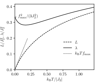
Figure 1: Temperature dependence of $L$ (dashed line) and $\lambda$ (solid line), in the isotropic model with $V(\mathbf{S})=0$, $f^{\alpha\beta}(x)=J(x^{2}-1)\delta^{\alpha\beta}$. The dotted line highlights the asymptotic behavior $L(T)\approx k_{\rm B}Tf_{\rm max}=k_{\rm B}T|J|$ for $T\to 0$.

The statistical mechanical properties of the model, computed from the equilibrium Gibbs distribution, are shown in Figs. 1, 2. In particular, Fig. 1 shows the temperature dependence of $L$ and $\lambda$, calculated numerically using Eq. (28), and the relations $L=-3/\beta^{2}-1/\sigma$, $\lambda=1/\sigma+\beta^{2}/(3\sigma^{2})$. In the limit of small temperatures, he variance $L=\langle\mathbf{b}_{i}^{2}\rangle^{\prime(i)}/3$ of the cavity distribution decreases with $T$ and vanishes for $T\to 0$ as $L(T)\approx k_{\rm B}Tf_{\rm max}=k_{\rm B}T|J|$. The full variance of the equilibrium distribution $\lambda=\langle\mathbf{b}_{i}^{2}\rangle/3$, instead, tends to $f^{2}_{\rm max}/3=|J|^{2}/3$ for $T\to 0$. In the opposite limit of high temperatures, $L\approx\lambda\approx{\cal J}_{2}^{2}/3=\sum_{j}J_{ij}^{2}/3=2|J|^{2}/3$.

The numerical solution shows a further interesting feature: the dependence of $\lambda$ on temperature is non-monotonic. $\lambda$ reaches a minimum at a temperature $T\simeq 0.167|J|$ and, for lower temperatures, starts to grow when $T$ is decreased.

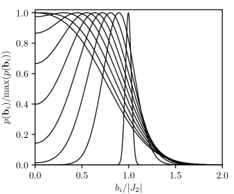
Figure 2: Equilibrium distribution of the field $\mathbf{b}_{i}$ for 10 different temperatures, equally spaced between $10^{-3}|J|$ and $0.25|J|$. At the higher temperatures in the plot, the distribution differs from a Gaussian, but has a bell-like shape with a maximum at $b_{i}=0$. At lower temperatures, the maximum shifts away from $b_{i}=0$. For $T\to 0$, the distribution becomes concentrated on a narrow shell near the spherical surface $|\mathbf{b}_{i}|=|J|=f_{\rm max}$.

The behavior ${\rm d}\lambda/{\rm d}T<0$ occurs in a region of temperatures for which the equilibrium distribution of the field $p(\mathbf{b}_{i})=\int_{\mathbf{S}}P(\mathbf{S}_{i},\mathbf{b}_{i})=\sinh(\beta|\mathbf{b}_{i}|)\exp[-(\beta^{2}L+L^{-1}\mathbf{b}_{i}^{2})/2]/[(2\pi L)^{3/2}\beta|\mathbf{b}_{i}|]$ is significantly different from a Gaussian function. The shape of the distribution $p(\mathbf{b}_{i})$ is shown in Fig. 2 for various temperatures.

The static properties are not sufficient to describe the system at low temperatures because a glass transition occurs. In the isotropic case the order-parameter equations reduce to:

$$\begin{split}&c_{1}=\frac{1}{3}-q_{\rm EA}=\frac{1}{\beta}I(\beta/\sigma_{1})~{},\\ &\beta^{2}c_{1}=-1/(\sigma_{1}^{-1}+L_{1})~{},\\ &q_{\rm EA}=\frac{1}{3}~{}\overline{\langle S^{\alpha}\rangle\langle S^{\alpha}\rangle}=\frac{1}{3}\overline{\big{(}{\cal L}(\beta|\mathbf{b}_{2}|)\big{)}^{2}}\\ &\quad~{}~{}=\frac{1}{3}(1-I_{1}(\beta^{2}L_{2}))~{},\\ &L=L_{1}+L_{2}~{},\end{split}$$ (71)

where ${\cal L}(x)=1/\tanh(x)-1/x$ is the Langevin function and

$$I_{1}(x)=\int_{-\infty}^{\infty}{\rm d}y~{}\frac{y[1-({\cal L}(y))^{2}]}{(2\pi x^{3})^{1/2}}\exp\bigg{(}-\frac{(y-x)^{2}}{2x}\bigg{)}~{}.$$ (72)

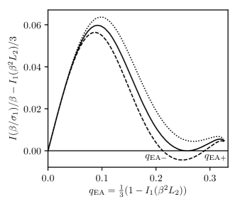
Figure 3: Numerical analysis of Eqs. (71). The curves show the function $I(\beta/\sigma_{1})/\beta-I_{1}(\beta^{2}L_{2})/3$ calculated substituting $\beta/\sigma_{1}=-1/(\beta c_{1})-\beta L_{1}=-3/(\beta I_{1}(\beta^{2}L_{2}))+\beta L_{2}-\beta L$. The $x$ axis is parametrized by the order parameter $q_{\rm EA}(\beta^{2}L_{2})=(1-I_{1}(\beta^{2}L_{2}))/3$. The dotted, solid, and dashed curves represent respectively the curves calculated at temperatures respectively equal to $T=0.012|J|/k_{\rm B}$, $0.0103|J|/k_{\rm B}$, and $0.009|J|/k_{\rm B}$. The solutions of the self-consistency problem are defined by the points at which the curves cross 0. For high-temperature the curve intersects 0 only at the trivial point $q_{\rm EA}=0$ (dotted line). A nontrivial solution appears at $T_{\rm g}\simeq 0.0103|J|/k_{\rm B}$. Below $T_{\rm g}$, the equations have two solutions $q_{{\rm EA}\pm}$. The physical solution is $q_{{\rm EA}+}$, the one with the largest order parameter.

A numerical study of the equations is presented in Fig. 3. At high temperatures, the only solution is the trivial one. However, at a temperature $T_{\rm g}\simeq 0.0103|J|/k_{\rm B}$ a nontrivial solution appears. We interpret $T_{\rm g}$ as the glass transition temperature, at which the system vitrifies. It is interesting to note that $T_{\rm g}$ is an order of magnitude smaller than the temperature scales which characterize the static solution. For example $T_{\rm g}$ is much smaller than the temperature $T\simeq 0.167|J|$ at which the derivative ${\rm d}\lambda/{\rm d}T$ changes sign.

At $T_{\rm g}$, the Edwards-Anderson order parameter $q_{\rm EA}$ jumps discontinuously from 0 to $q_{\rm EA}(T_{\rm g})\simeq 0.2575$. The jump is large: the magnetization of a spin at $T_{\rm g}$, $|\mathbf{m}|=[\overline{\langle S^{\alpha}\rangle\langle S^{\alpha}\rangle}]^{1/2}=\sqrt{3q_{\rm EA}(T_{\rm g})}\simeq 0.879$ is at $T_{\rm g}$ already close to the saturation value $|\mathbf{m}|=1$. Below $T_{\rm g}$ Eqs. (71) present two solutions $q_{{\rm EA}\pm}(T)$, which bifurcate from the transition point. The physical solution is the one with the largest overlap, which we denote as $q_{{\rm EA}+}(T)$. The other branch $q_{{\rm EA}-}(T)$ cannot be physical because it leads to an order parameter which decreases when $T$ is lowered. The temperature dependence of the solution $q_{\rm EA}(T)=q_{{\rm EA}+}(T)$ is illustrated in Fig. 4. Starting from the transition point, $q_{\rm EA}(T_{\rm g})$ grows at small $T$ and eventually reaches $1$ for $T\to 0$.

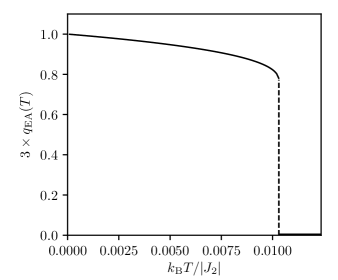
Figure 4: Equilibrium average of the Edwards-Anderson order parameter $q_{\rm EA}(T)$ obtained from a numerical solution of Eqs. (71). The order parameter represented in the figure describes the large-time limit $3q_{\rm EA}(T)=\lim_{|t-t^{\prime}|\to\infty}\langle S^{\alpha}(t)S^{\alpha}(t^{\prime})\rangle$, with an averaging $\langle...\rangle$ weighted with the equilibrium Gibbs distribution at temperature $T$. This equilibrium $q_{\rm EA}$ may differ in general from the average order parameter which the system presents after a cooling from the paramagnetic phase $T>T_{\rm g}$, because the spins remain trapped in a single metastable state at $T_{\rm g}$ and fall out of equilibrium at lower temperatures.

The transition is of a dynamical first order type, similar to the transition which occurs in supercooled liquids in $d\to\infty$ [58] and which was predicted in stripe systems [8, 9, 10, 11, 12, 13, 14]. In fact at $T_{\rm g}$, the equilibrium statistical properties remain smooth, without any signature of a phase transition, but the system undergoes a dynamical arrest. This contrasts, for example, with the second-order transitions found in random spin glasses [3]. Below $T_{\rm g}$ the system remains trapped into a single metastable state and thus falls out of equilibrium. After cooling from the high temperature liquid regime $T>T_{\rm g}$ to the glassy region $T<T_{\rm g}$, we can expect that the physical thermal properties are not controlled by the equilibrium distribution at $T$, but by the distribution of metastable states at the temperature at $T_{\rm g}$, at which the system fell out of equilibrium for the first time. The replica theory is useful to discuss this regime [36]. Another question which remains open is whether the Heisenberg model presents at a temperature $T_{\rm s}<T_{\rm g}$ a static glass transition, similarly to the Ising model analyzed in Ref. [36].

VII Conclusions

In this article, we have analyzed a class of exactly solvable frustrated spin models, characterized by the property that their interaction $J(\mathbf{k})$ presents a degenerate surface of maxima in momentum space. Using the cavity method, we derived in the limit of infinite dimensionality $d\to\infty$ the exact solution of the statistical mechanical properties in the paramagnetic phase. By a study of the equilibrium dynamics of the system, we derived a set of consistency equations for the glass order parameters. The theory was applied explicitly to the case of a isotropic model, equivalent after bipartition of the hypercubic lattice to a Heisenberg model on the fcc lattice. For this model we identified the temperature of dynamical vitrification. The transition is of a dynamical first order type and is similar to the vitrification predicted in the theory of stripe glassiness. Although the exact results were obtained in the limit of infinite dimensions, the power demonstrated by DMFT methods in describing correlated electron systems [44, 45, 46] indicates the relevance of the results also for the realistic case of a system in three dimensions. In comparison to the previous works hypothesizing self-induced spin-glass states in deterministic frustrated spin models [16, 15] our new approach seems to have two advantages. First, it has an explicit small parameter, albeit formal, and second it does not use the replica trick, whose applicability for deterministic systems is not obvious. Instead, we study the large-time behavior of correlation functions, in the spirit of the original approach by Edwards and Anderson in the theory of spin glasses, and Götze mode-coupling theory in the context of structural glasses. Importantly, both approaches lead to the same conclusion that frustration only can be sufficient for vitrification. This qualitatively supports the interpretation of the experimental data of Refs. [34, 35] as an observation of a self-induced spin glass state in elemental neodymium at low temperatures. Another interesting technical question concerning the relation between dynamical and replica approaches will be considered elsewhere.

Appendix A Fokker-Planck equation and fluctuation-dissipation theorem

The Fokker-Planck (FP) equation associated with the Brownian motion of magnetic moments has been discussed in several works (see for example Refs. [60, 61, 55, 62]).

Here we give a brief derivation of the FP equation, and discuss the FDT and the Hilbert space representation of the dynamics. To derive the equations, we parametrize the spins by two coordinates $(\theta^{1}_{i},\theta^{2}_{i})$. A natural choice are the spherical coordinates $\theta^{1}_{i}=\theta_{i}$, $\theta_{i}^{2}=\varphi_{i}$, $\mathbf{S}(\theta^{1},\theta^{2})=(\sin\theta^{1}\cos\theta^{2},\sin\theta^{1}\sin\theta^{2},\cos\theta^{1})$, but an arbitrary pametrization can be used. In the following we denote as $\theta^{\mu}_{i}$, $\mu=1,2$ the coordinates. To avoid confusion, letters from the beginning of the Greek alphabet $\alpha$, $\beta$, $\gamma$, $\delta$ are used to denote the cartesian components of the spins, as in the main text; letters from the final part of the alphabet $\mu$, $\nu$, $\rho$, … are used, instead, to denote the two-dimensional parametrization $\theta^{\mu}$.

In terms of the $\theta^{\mu}_{i}$, the Langevin equation can be written as:

$$\dot{\theta}^{\mu}_{i}=g^{\mu\nu}(\bm{\theta}_{i})(\mathbf{u}_{\nu}(\bm{\theta}_{i})\cdot\mathbf{E}_{i})~{},$$ (73)

where $\mathbf{E}_{i}=-\mathbf{S}_{i}\times(\mathbf{S}_{i}\times(\mathbf{N}_{i}+\bm{\nu}_{i}))$ is the right-hand side of the equation of motion (30), $\mathbf{u}_{\mu}(\bm{\theta})=\partial\mathbf{S}/\partial\theta^{\mu}$ are the tangent vectors, and $g^{\mu\nu}(\bm{\theta})$ is the inverse of the metric tensor $g_{\mu\nu}(\bm{\theta})=(\mathbf{u}_{\mu}(\bm{\theta})\cdot\mathbf{u}_{\nu}(\bm{\theta}))$.

Using the theory of Langevin processes on manifolds [59] and introducing the reparametrization-invariant distribution

$$\rho(\bm{\theta}_{1},....,\bm{\theta}_{N})=\frac{\left\langle\prod_{i=1}^{N}\delta(\bm{\theta}_{i}-\bm{\theta}_{i}(t))\right\rangle_{\bm{\nu}}}{\prod_{j=1}^{N}\sqrt{g(\bm{\theta}_{j})}}$$ (74)

we find after some computations:

$$\begin{split}&\frac{\partial\rho}{\partial t}+\sum_{i=1}^{N}\frac{1}{\sqrt{g(\bm{\theta}_{i})}}\frac{\partial}{\partial\theta_{i}^{\mu}}\bigg{\{}\sqrt{g(\bm{\theta}_{i})}g^{\mu\nu}(\bm{\theta}_{i})\\ &\times\bigg{[}(\mathbf{u}_{\nu}(\bm{\theta}_{i})\cdot\mathbf{N}_{i})\rho-k_{\rm B}T\frac{\partial\rho}{\partial\theta_{i}^{\nu}}\bigg{]}\bigg{\}}=0~{}.\end{split}$$ (75)

In Eq. (74) the factor $1/\prod_{j=1}^{N}\sqrt{g(\bm{\theta}_{j})}$, $g(\bm{\theta}_{i})=\det g_{\mu\nu}(\bm{\theta}_{i})$ is introduced in order to make the probability invariant. With this normalization $\rho$ is the invariant probability distribution. It gives the probability to find the system in an infinitesimal element ${\rm d}\Omega$ of the configuration space: ${\rm d}P=\rho(\bm{\theta}_{1},..,\bm{\theta}_{N}){\rm d}\Omega=\rho(\bm{\theta}_{1},..,\bm{\theta}_{N})\prod_{i}\sqrt{g(\bm{\theta}_{i})}{\rm d}^{2}\theta_{i}$.

In spherical coordinates $g(\bm{\theta}_{i})=\sin^{2}\theta_{i}$ and the infinitesimal element is the usual ${\rm d}\Omega=\prod_{i=1}^{N}\sin\theta_{i}{\rm d}\theta_{i}{\rm d}\varphi_{i}$. Eq. (75) becomes in these coordinates:

$$\begin{split}&\frac{\partial\rho}{\partial t}+\sum_{i=1}^{N}\bigg{\{}\frac{1}{\sin\theta_{i}}\frac{\partial}{\partial\theta_{i}}\bigg{[}\sin\theta_{i}\bigg{(}(N_{i}^{x}\cos\theta_{i}\cos\varphi_{i}\\ &+N_{i}^{y}\cos\theta_{i}\sin\varphi_{i}-N_{i}^{z}\sin\theta_{i})\rho-k_{\rm B}T\frac{\partial\rho}{\partial\theta_{i}}\bigg{)}\bigg{]}\\ &+\frac{1}{\sin^{2}\theta_{i}}\frac{\partial}{\partial\varphi_{i}}\bigg{[}(-N_{i}^{x}\sin\varphi_{i}+N_{i}^{y}\cos\varphi_{i})\sin\theta_{i}\rho\\ &\qquad-k_{\rm B}T\frac{\partial\rho}{\partial\varphi_{i}}\bigg{]}\bigg{\}}=0~{}.\end{split}$$ (76)

As a remark, we note that the methodolody which leads to Eq. (75) assumes the Stratonovich stochastic calculus. Thus in Eq. (30) we implicitly assume a Langevin equation (30) defined according to the Stratonovich prescription (see Ref. [62] for different prescriptions).

The time evolution can be written more compactly introducing the angular momentum operators [61], which in a general frame of coordinates can be written as:

$$\begin{split}\bm{\mathscr{L}}^{\alpha}_{i}\bullet&=-i\epsilon^{\alpha\beta\gamma}g^{\mu\nu}(\bm{\theta}_{i})(S^{\beta}_{i}u^{\gamma}_{\mu}(\bm{\theta}_{i}))\frac{\partial}{\partial\theta_{i}^{\nu}}\bullet\\ &=-\frac{i\epsilon^{\alpha\beta\gamma}}{\sqrt{g(\bm{\theta}_{i})}}\frac{\partial}{\partial\theta_{i}^{\nu}}\sqrt{g(\bm{\theta}_{i})}g^{\mu\nu}(\bm{\theta}_{i})S^{\beta}_{i}u_{\mu}^{\gamma}(\bm{\theta}_{i})\bullet~{}.\end{split}$$ (77)

These are generators of spin rotations and satisfy the commutation relations $[\mathscr{L}^{\alpha}_{i},S^{\beta}_{j}]=i\delta_{ij}\epsilon^{\alpha\beta\gamma}S^{\gamma}_{i}$, $[\mathscr{L}^{\alpha}_{i},\mathscr{L}^{\beta}_{j}]=i\delta_{ij}\epsilon^{\alpha\beta\gamma}\mathscr{L}_{i}^{\gamma}$. Note that $[S^{\alpha}_{i},S^{\beta}_{j}]=0$ because the spins here are simply classical variables.

In terms of the $\mathscr{L}_{i}^{\alpha}$, the FP equation (75) can be recast as:

$$\begin{split}\frac{\partial\rho}{\partial t}&+\mathscr{H}\rho=0~{},\end{split}$$ (78)

with

$$\begin{split}\mathscr{H}&=\sum_{i=1}^{N}\mathscr{L}_{i}^{\alpha}(i\epsilon^{\alpha\beta\gamma}S^{\beta}_{i}N^{\gamma}_{i}+k_{\rm B}T\mathscr{L}^{\alpha}_{i})~{}.\end{split}$$ (79)

and the components of the angular momentum operators read as usual

$$\begin{split}\mathscr{L}_{i}^{x}&=i\sin\varphi_{i}\frac{\partial}{\partial\theta_{i}}+\frac{i\cos\varphi_{i}}{\tan\theta_{i}}\frac{\partial}{\partial\varphi_{i}}~{},\\ \mathscr{L}_{i}^{y}&=-i\cos\varphi_{i}\frac{\partial}{\partial\theta_{i}}+\frac{i\sin\varphi_{i}}{\tan\theta_{i}}\frac{\partial}{\partial\varphi_{i}}~{},\\ \mathscr{L}_{i}^{z}&=-i\frac{\partial}{\partial\varphi_{i}}~{}.\end{split}$$ (80)

Using that $\mathscr{L}_{i}^{\alpha}H=i\epsilon^{\alpha\beta\gamma}S^{\beta}_{i}N_{i}^{\gamma}$, it is simple to show that the operator $i\epsilon^{\alpha\beta\gamma}S^{\beta}_{i}N^{\gamma}_{i}+k_{\rm B}T\mathscr{L}_{i}^{\alpha}$ annihilates the Gibbs distribution $\rho_{\rm G}=Z^{-1}{\rm e}^{-\beta H}$. Thus, $\rho_{\rm G}$ is stationary in time: $\partial\rho_{\rm G}/\partial t=-\mathscr{H}\rho_{\rm G}=0$.

Time-dependent correlation functions can be studied by setting up a Hilbert-space representation [59, 63]. Here, in order to maintain a notation which is manifestly reparametrization invariant, we find it convenient to define the scalar product of two functions $|\Phi_{1}\rangle=\Phi_{1}(\bm{\theta}_{1},...,\bm{\theta}_{N})$, $|\Phi_{2}\rangle=\Phi_{2}(\bm{\theta}_{1},...,\bm{\theta}_{N})$ as $\langle\Phi_{1}|\Phi_{2}\rangle=\int\prod_{j}{\rm d}^{2}\theta_{j}\sqrt{g(\bm{\theta}_{j})}\Phi^{*}_{1}(\bm{\theta}_{1},..,\bm{\theta}_{N})\Phi_{2}(\bm{\theta}_{1},...,\bm{\theta}_{N})$, including in the definition of the product the measure $\sqrt{g}$. (In spherical coordinates $\sqrt{g(\theta,\varphi)}=\sin\theta$ and the integrals are the usual $\int{\rm d}^{2}\theta_{j}\sqrt{g(\bm{\theta}_{j})}=\int_{0}^{\pi}{\rm d}\theta_{j}\int_{0}^{2\pi}{\rm d}\varphi_{j}\sin\theta_{j}$).

If the distribution of the initial conditions at time $t=0$ is $|\rho\rangle$, the average of a product of spin variables at later times can be represented as:

$$\begin{split}\langle S_{i_{1}}^{\alpha_{1}}(t_{1})&...S^{\alpha_{l}}_{i_{l}}(t_{l})\rangle=\langle 1|S_{i_{1}}^{\alpha_{1}}{\rm e}^{-\mathscr{H}(t_{1}-t_{2})}\times\\ &...\times{\rm e}^{-\mathscr{H}(t_{l-1}-t_{l})}S_{i_{l}}^{\alpha_{l}}{\rm e}^{-\mathscr{H}t_{l}}|\rho\rangle~{},\end{split}$$ (81)

where it is assumed that the times are arranged in the order as $t_{1}>t_{2}>...>t_{l}>0$. $|1\rangle$ is simply a function equal to 1, so that the scalar product $\langle 1|\Phi\rangle$ is the integral of $\Phi(\bm{\theta}_{1},..,\bm{\theta}_{N})$ over the configuration space, computed with the invariant measure $\prod_{j}{\rm d}^{2}\theta_{j}\sqrt{g(\bm{\theta}_{j})}$. In particular, the condition that $|\rho\rangle$ is normalized is expressed by $\langle 1|\rho\rangle=1$.

It can be verified that $\langle 1|\mathscr{L}^{\alpha}_{i}=0$. In fact, for any function $|\Phi\rangle$ Eq. (77) implies:

$$\begin{split}\langle 1|\mathscr{L}^{\alpha}_{i}|\Phi\rangle&=-i\epsilon^{\alpha\beta\gamma}\int\prod_{j=1}^{N}{\rm d}^{2}\theta_{j}\frac{\partial}{\partial\theta_{i}^{\nu}}[\sqrt{g}(\bm{\theta}_{i})\\ &\times g^{\mu\nu}(\bm{\theta}_{i})S^{\beta}_{i}u_{\mu}^{\gamma}\Phi(\bm{\theta}_{1},..,\bm{\theta}_{N})]=0~{},\end{split}$$ (82)

which vanishes because it is a total divergence, and the configuration space has no boundary. The relation $\langle 1|\mathscr{L}^{\alpha}_{i}$ implies that $\langle 1|\mathscr{H}=0$, that is, $\langle 1|$ is a left eigenvector with zero eigenvalue. THis implies in particular that $\langle 1|{\rm e}^{-\mathscr{H}t}=\langle 1|$, which is the conservation of probability: $\langle 1|\rho(t)\rangle=\langle 1|{\rm e}^{-\mathscr{H}t}|\rho\rangle=\langle 1|\rho\rangle=1$.

Similarly, the Gibbs distribution $|\rho_{\rm G}\rangle$ is a right-eigenvector with zero eigenvalue: $\mathscr{H}|\rho_{\rm G}\rangle=0$. In addition for all $i$, $(i\epsilon^{\alpha\beta\gamma}S^{\beta}_{i}N^{\gamma}_{i}+k_{\rm B}T\mathscr{L}_{i}^{\alpha})|\rho_{\rm G}\rangle=0$. These relations allow to write the correlations in the form [59]

$$\langle S_{i_{1}}^{\alpha_{1}}(t_{1})...S^{\alpha_{l}}_{i_{l}}(t_{l})\rangle=\left\langle 1\left|T\{\mathscr{S}^{\alpha_{1}}_{i_{1}}(t_{1})...\mathscr{S}^{\alpha_{l}}_{i_{l}}(t_{l})\}\right|\rho_{\rm G}\right\rangle~{},$$ (83)

where $\mathscr{S}^{\alpha}_{i}(t)={\rm e}^{\mathscr{H}t}S_{i}^{\alpha}{\rm e}^{-\mathscr{H}t}$ and $T$ is the time-ordering operator.

In this representation, the FDT is encoded by the fact that the time-derivative of the correlation function, in the region $t>t^{\prime}$, is

$$\begin{split}&\frac{{\rm d}}{{\rm d}t}\langle S^{\alpha}_{i}(t)S^{\beta}_{j}(t^{\prime})\rangle=\big{\langle}1\big{|}[\mathscr{H},\mathscr{S}^{\alpha}_{i}(t)]\mathscr{S}^{\beta}_{j}(t^{\prime})\big{|}\rho_{\rm G}\big{\rangle}\\ &=-\big{\langle}1\big{|}\mathscr{S}_{i}^{\alpha}(t-t^{\prime})[\mathscr{H},S_{j}^{\beta}]\big{|}\rho_{\rm G}\big{\rangle}\\ &=ik_{\rm B}T\epsilon^{\beta\gamma\delta}\big{\langle}1\big{|}\mathscr{S}_{i}^{\alpha}(t-t^{\prime})\mathscr{L}^{\gamma}_{j}(0)\mathscr{S}_{j}^{\delta}(0)\big{|}\rho_{\rm G}\big{\rangle}~{},\end{split}$$ (84)

and is proportional to the Kubo formula for the linear response function $G^{\alpha\beta}_{ij}=\langle\delta S^{\alpha}_{i}(t)/\delta\nu_{j}^{\beta}(t^{\prime})\rangle$:

$$\begin{split}G^{\alpha\beta}_{ij}(t-t^{\prime})&=-i\epsilon^{\beta\gamma\delta}\big{\langle}1\big{|}\mathscr{S}^{\alpha}_{i}(t-t^{\prime})\mathscr{L}_{j}^{\gamma}(0)\mathscr{S}_{j}^{\delta}(0)\big{|}\rho_{\rm G}\big{\rangle}\\ &=-\beta\Theta(t-t^{\prime})\frac{{\rm d}}{{\rm d}t}\langle S^{\alpha}_{i}(t)S^{\beta}_{j}(t^{\prime})\rangle~{}.\end{split}$$ (85)

Eq. (85) follows from the general formulas of linear response theory. It can be derived by using that in presence of a small external field $\delta\nu_{j}^{\alpha}(t)$ the FP evolution equations become $\partial\rho/\partial t+\mathscr{H}\rho+\mathscr{H}_{1}(t)\rho=0$ with $\mathscr{H}_{1}(t)=i\epsilon^{\alpha\beta\gamma}\sum_{i=1}^{N}\mathscr{L}_{i}^{\alpha}S_{i}^{\beta}\delta\nu_{i}^{\gamma}(t)$. The perturbation $\mathscr{H}_{1}(t)$ describes the effect on the motion of the field $\delta\nu_{i}^{\alpha}(t)$ which modifies $\mathbf{N}_{i}\to\mathbf{N}_{i}+\bm{\nu}_{i}$.

In analogy with other purely-dissipative equations [59, 63], it is also useful to discuss the FP equation by performing the transformation $\rho\to\tilde{\rho}$, $\rho={\rm e}^{-\beta H/2}\tilde{\rho}$. The transformed operators are:

$$\begin{gathered}\tilde{\mathscr{L}}^{\alpha}_{i}={\rm e}^{\beta H/2}\mathscr{L}^{\alpha}_{i}{\rm e}^{-\beta H/2}=\mathscr{L}^{\alpha}_{i}-\frac{i}{2}\beta\epsilon^{\alpha\beta\gamma}S_{i}^{\beta}N_{i}^{\gamma}~{},\\ \tilde{S}^{\alpha}_{i}={\rm e}^{\beta H/2}\mathscr{L}^{\alpha}_{i}{\rm e}^{-\beta H/2}=S_{i}^{\alpha}~{},\\ \tilde{\mathscr{H}}={\rm e}^{\beta H/2}\mathscr{H}{\rm e}^{-\beta H/2}=k_{\rm B}T\sum_{i=1}^{N}\tilde{\mathscr{L}}_{i}^{\alpha}\tilde{\mathscr{L}}_{i}^{\alpha+}~{}.\end{gathered}$$ (86)

Here $\tilde{\mathscr{L}}^{\alpha+}_{i}=\mathscr{L}^{\alpha}_{i}+i\beta\epsilon^{\alpha\beta\gamma}S_{i}^{\beta}N_{i}^{\gamma}/2$ is the adjoint of $\tilde{\mathscr{L}}^{\alpha}_{i}$ ($\mathscr{L}^{\alpha}_{i}$ and $S_{i}^{\alpha}$ are self-adjoint). In this representation $\tilde{\mathscr{H}}$ is Hermitian, and has the same left and right eigenvectors. By contrast the evolution operator $\mathscr{H}$ before the transformation is not Hermitian [59]. Eq. (86) also shows that $\tilde{\mathscr{H}}$ is positive semidefinite: all eigenvalues of $\tilde{\mathscr{H}}$ are $\geq 0$. The Gibbs distribution $|\tilde{\rho}_{\rm G}\rangle={\rm e}^{\beta H/2}|\rho_{\rm G}\rangle$ is a ground state and satisfies $\tilde{\mathscr{L}}^{\alpha+}_{i}|\tilde{\rho}_{\rm G}\rangle=0$.

Appendix B Dynamical two-point correlations

The derivation in Sec. IV.3 implies that any dynamical correlation of $\mathbf{S}_{i}$, $\mathbf{b}_{i}$, $\mathbf{S}_{j}$, $\mathbf{b}_{j}$ can be calculated replacing the definitions $b^{\alpha}_{i}(t)=\sum_{k}J_{ik}^{\alpha\beta}S^{\beta}_{k}(t)$, $b^{\alpha}_{j}(t)=\sum_{k}J_{ik}^{\alpha\beta}S^{\beta}_{k}(t)$, with Eqs. (56). In more detail, we can calculate the second-order correlations as:

$$\begin{split}C^{\alpha\beta}_{ij}(t-t^{\prime})&=\langle S^{\alpha}_{i}(t)S^{\beta}_{i}(t^{\prime})\rangle_{\bm{\nu}_{i},\bm{\nu}_{j},\bm{\zeta}_{i},\bm{\zeta}_{j},\mathbf{S}_{i0},\mathbf{S}_{j0}}~{},\\ A^{\alpha\beta}_{ij}(t-t^{\prime})&=\langle S^{\alpha}_{i}(t)b^{\beta}_{i}(t^{\prime})\rangle_{\bm{\nu}_{i},\bm{\nu}_{j},\bm{\zeta}_{i},\bm{\zeta}_{j},\mathbf{S}_{i0},\mathbf{S}_{j0}}~{},\\ \Lambda^{\alpha\beta}_{ij}(t-t^{\prime})&=\langle b^{\alpha}_{i}(t)b^{\beta}_{i}(t^{\prime})\rangle_{\bm{\nu}_{i},\bm{\nu}_{j},\bm{\zeta}_{i},\bm{\zeta}_{j},\mathbf{S}_{i0},\mathbf{S}_{j0}}~{},\\ \end{split}$$ (87)

where $\mathbf{S}_{i}(t)$, $\mathbf{S}_{j}(t)$, $\mathbf{b}_{i}(t)$, $\mathbf{b}_{j}(t)$ are solutions of the two-site Langevin equations $\dot{\mathbf{S}}_{i}=-\mathbf{S}_{i}\times(\mathbf{S}_{i}\times(\mathbf{F}(\mathbf{S}_{i})+\mathbf{b}_{i}+\bm{\nu}_{i}))$, $\dot{\mathbf{S}}_{j}=-\mathbf{S}_{j}\times(\mathbf{S}_{j}\times(\mathbf{F}(\mathbf{S}_{j})+\mathbf{b}_{j}+\bm{\nu}_{j}))$, with the fields $\mathbf{b}_{i}$ and $\mathbf{b}_{j}$ in Eqs. (56). The correlations are determined by averaging the solutions over the noises $\bm{\nu}_{i}$, $\bm{\nu}_{j}$, $\bm{\zeta}_{i}$, $\bm{\zeta}_{j}$, and over the initial conditions $\mathbf{S}_{i0}$, $\mathbf{S}_{j0}$ of the two spins.

Let us first analyze the correlation $C^{\alpha\beta}_{ij}(t-t^{\prime})$. Since $r_{ij}$, $R_{ij}$, and $J_{ij}$ are small ($\approx d^{-\ell_{ij}/2}$), the spins are only weakly coupled. For any fixed realization of the noises and the initial conditions the trajectories can be expanded to first order as:

$$\begin{split}&S^{\alpha}_{i}(t)=\tilde{S}^{\alpha}_{i}(t)+\int_{0}^{t}{\rm d}t^{\prime\prime}~{}\tilde{G}_{i}^{\alpha,\gamma}(t,t^{\prime\prime})\Delta b_{i}^{\gamma}(t^{\prime\prime})~{},\\ &S^{\alpha}_{j}(t)=\tilde{S}^{\alpha}_{j}(t)+\int_{0}^{t}{\rm d}t^{\prime\prime}~{}\tilde{G}_{j}^{\alpha,\gamma}(t,t^{\prime\prime})\Delta b_{j}^{\gamma}(t^{\prime\prime})~{},\\ &\Delta b^{\gamma}_{i}(t^{\prime\prime})=J_{ij}^{\gamma\delta}\tilde{S}_{j}^{\delta}(t^{\prime\prime})+\beta r^{\gamma\delta}_{ij}(t^{\prime\prime})S^{\delta}_{j0}\\ &\qquad+\int_{0}^{t^{\prime\prime}}{\rm d}t^{\prime\prime\prime}~{}R^{\gamma\delta}_{ij}(t^{\prime\prime}-t^{\prime\prime\prime})\tilde{S}_{j}^{\delta}(t^{\prime\prime\prime})~{},\\ &\Delta b^{\gamma}_{j}(t^{\prime\prime})=J_{ji}^{\gamma\delta}\tilde{S}_{i}^{\delta}(t^{\prime\prime})+\beta r^{\gamma\delta}_{ji}(t^{\prime\prime})S^{\delta}_{i0}\\ &\qquad+\int_{0}^{t^{\prime\prime}}{\rm d}t^{\prime\prime\prime}~{}R^{\gamma\delta}_{ji}(t^{\prime\prime}-t^{\prime\prime\prime})\tilde{S}_{i}^{\delta}(t^{\prime\prime\prime})~{}.\\ \end{split}$$ (88)

Here $\tilde{\mathbf{S}}_{i}(t)$, $\tilde{\mathbf{S}}_{j}(t)$ are solutions of the single-site Langevin equations

$$\begin{split}\dot{\tilde{\mathbf{S}}}_{i}&=-\tilde{\mathbf{S}}_{i}\times(\tilde{\mathbf{S}}_{i}\times(\mathbf{F}(\tilde{\mathbf{S}_{i}})+\tilde{\mathbf{b}}_{i}(t)+\bm{\nu}_{i}))~{},\\ \dot{\tilde{\mathbf{S}}}_{j}&=-\tilde{\mathbf{S}}_{j}\times(\tilde{\mathbf{S}}_{j}\times(\mathbf{F}(\tilde{\mathbf{S}}_{j})+\tilde{\mathbf{b}}_{j}(t)+\bm{\nu}_{j}))~{},\\ \tilde{b}^{\alpha}_{i}(t)&=\bm{\zeta}_{i}(t)+\beta l^{\alpha\beta}S^{\beta}_{i0}+\int_{0}^{t^{\prime\prime}}~{}K^{\alpha\gamma}(t-t^{\prime\prime})\tilde{S}^{\beta}_{i}(t^{\prime\prime})~{},\\ \tilde{b}^{\alpha}_{j}(t)&=\bm{\zeta}_{j}(t)+\beta l^{\alpha\beta}S^{\beta}_{j0}+\int_{0}^{t^{\prime\prime}}~{}K^{\alpha\gamma}(t-t^{\prime\prime})\tilde{S}^{\beta}_{j}(t^{\prime\prime})~{},\end{split}$$ (89)

and $\tilde{G}^{\alpha\beta}_{i}(t,t^{\prime})$, $\tilde{G}^{\alpha\beta}_{i}(t,t^{\prime})$ are the corresponding response functions.

To find $C^{\alpha\beta}_{ij}(t-t^{\prime})$ we need to discuss the averaging over initial conditions and over the noise. Since we are studying equilibrium correlations, the initial conditions must be weighted with the joint probability $P_{2}(\mathbf{S}_{i0},\mathbf{S}_{j0})$ to extract given values $\mathbf{S}_{i0}$ and $\mathbf{S}_{j0}$ of two spins in the Gibbs distribution. This probability can be calculated as:

$$P_{2}(\mathbf{S}_{i0},\mathbf{S}_{j0})=\int{\rm d}^{3}\bar{\mathbf{b}}_{i}\int{\rm d}^{3}\bar{\mathbf{b}}_{j}P(\mathbf{S}_{i0},\bar{\mathbf{b}}_{i};\mathbf{S}_{j0},\bar{\mathbf{b}}_{j})$$ (90)

where $P(\mathbf{S}_{i},\mathbf{b}_{i};\mathbf{S}_{j},\mathbf{b}_{j})$ is the distribution found in the static computation [Eqs. (17) and (19)]. At leading order for $d\to\infty$, it is sufficient to expand the distribution (19) at first order in $J^{\alpha\beta}_{ij}$ and $M^{\alpha\beta}_{ij}$. After integration over the magnetic fields we find:

$$\begin{split}P_{2}(\mathbf{S}_{i0},\mathbf{S}_{j0})&=P_{1{\rm}}(\mathbf{S}_{i0})P_{1{\rm eq}}(\mathbf{S}_{j0})(1+\beta J^{\alpha\beta}_{ij}S^{\alpha}_{i0}S^{\beta}_{j0}\\ &-\beta^{2}L^{\alpha\gamma}M_{ij}^{\gamma\delta}L^{\delta\beta}S^{\alpha}_{i0}S^{\beta}_{j0})~{}.\end{split}$$ (91)

The static equation (19), on the other hand implies that the fields $X^{\alpha}_{1}=\sum_{k\neq i,j}J^{\alpha\beta}_{ik}S^{\beta}_{k}$, $X^{\alpha}_{2}=\sum_{k\neq i,j}J^{\alpha\beta}_{jk}S^{\beta}_{k}$ have a correlation $\mathopen{\hbox{${\langle}$}\kern-1.94444pt\leavevmode\hbox{${\langle}$}}X^{\alpha}_{1}X^{\alpha}_{2}\mathclose{\hbox{${\rangle}$}\kern-1.94444pt\leavevmode\hbox{${\rangle}$}}^{\prime\prime(ij)}\approx-L^{\alpha\gamma}M_{ij}^{\gamma\delta}L^{\delta\beta}$ when they are averaged with the statistical distribution of the cavity system. $X^{\alpha}_{1}$ and $X^{\alpha}_{2}$ play the same role of $\zeta_{i}^{\alpha}$ and $\zeta_{j}^{\alpha}$, the Gaussian noises which enter the dynamical equations (56). We can thus identify $\mathopen{\hbox{${\langle}$}\kern-1.94444pt\leavevmode\hbox{${\langle}$}}X^{\alpha}_{1}X^{\alpha}_{2}\mathclose{\hbox{${\rangle}$}\kern-1.94444pt\leavevmode\hbox{${\rangle}$}}^{\prime\prime(ij)}$ with the equal-time element $r^{\alpha\beta}_{ij}(0)$ of the correlation $r_{ij}^{\alpha\beta}(t-t^{\prime})$. As a result we can write the equilibrium distribution of the initial conditions as: $P_{2}(\mathbf{S}_{i0},\mathbf{S}_{j0})=P_{1{\rm eq}}(\mathbf{S}_{i0})P_{1{\rm eq}}(\mathbf{S}_{j0})(1+\beta J^{\alpha\beta}_{ij}S^{\alpha}_{i0}S^{\beta}_{j0}+\beta^{2}r_{ij}^{\alpha\beta}(0)S^{\alpha}_{i0}S^{\beta}_{j0})$, where $P_{1{\rm eq}}(\mathbf{S}_{i0})$ is the single-site probability [Eq. (35)].

Consider now the distribution of the noise. We can formally write the Gaussian probability $P_{2{\rm noise}}[\bm{\zeta}_{i},\bm{\zeta}_{j}]$ of a given realization $\bm{\zeta}_{i}(t)$, $\bm{\zeta}_{j}(t)$ in the form:

$$\begin{split}&P_{2{\rm noise}}[\bm{\zeta}_{i},\bm{\zeta}_{j}]={\cal N}_{2}\exp\Big{[}-\frac{1}{2}{\textstyle\int}_{0}^{\infty}{\textstyle\int}_{0}^{\infty}{\rm d}t{\rm d}t^{\prime}~{}\\ &\qquad{\textstyle\sum}_{a=i,j}{\textstyle\sum}_{b=i,j}~{}l^{-1\alpha\beta}_{ab}(t-t^{\prime})\zeta^{\alpha}_{a}(t)\zeta^{\beta}_{b}(t^{\prime})\Big{]}~{},\end{split}$$ (92)

where $l^{-1\alpha\beta}_{ab}(t-t^{\prime})$ is the inverse of the matrix

$$\begin{split}l^{\alpha\beta}_{ab}(t-t^{\prime})&=\begin{Vmatrix}l^{\alpha\beta}_{ii}(t-t^{\prime})&l_{ij}^{\alpha\beta}(t-t^{\prime})\\ l_{ji}^{\alpha\beta}(t-t^{\prime})&l_{jj}^{\alpha\beta}(t-t^{\prime})\end{Vmatrix}\\ &=\begin{Vmatrix}l^{\alpha\beta}(t-t^{\prime})&r_{ij}^{\alpha\beta}(t-t^{\prime})\\ r_{ji}^{\alpha\beta}(t-t^{\prime})&l^{\alpha\beta}(t-t^{\prime})\end{Vmatrix}~{},\end{split}$$ (93)

and ${\cal N}_{2}$ is a normalization constant. The inverse is intended in the sense of kernels: $\sum_{c}\int_{0}^{\infty}{\rm d}t^{\prime\prime}~{}l^{-1\alpha\gamma}_{ac}(t-t^{\prime\prime})l^{\gamma\beta}_{cb}(t^{\prime\prime}-t^{\prime})=\delta^{\alpha\beta}\delta_{ab}\delta(t-t^{\prime})$.

Expanding to first order in $r_{ij}$ we find:

$$\begin{split}&P_{2{\rm noise}}[\bm{\zeta}_{i},\bm{\zeta}_{j}]\simeq P_{1{\rm noise}}[\bm{\zeta}_{1}]P_{1{\rm noise}}[\bm{\zeta}_{1}]\\ &\times\Big{[}1+{\textstyle\int}_{0}^{\infty}{\rm d}t{\textstyle\int}_{0}^{\infty}{\rm d}t^{\prime\prime}{\textstyle\int}_{0}^{\infty}{\rm d}t_{1}{\textstyle\int}_{0}^{\infty}{\rm d}t_{2}\big{(}l^{-1\alpha\gamma}(t-t_{1})\\ &\times r_{ij}^{\gamma\delta}(t_{1}-t_{2})l^{-1\delta\beta}(t_{2}-t^{\prime})\zeta^{\alpha}_{i}(t)\zeta^{\beta}_{j}(t^{\prime})\big{)}\Big{]}~{},\end{split}$$ (94)

where

$$\begin{split}P_{1{\rm noise}}[\bm{\zeta}]&={\cal N}_{1}\exp\Big{[}-\frac{1}{2}{\textstyle\int}_{0}^{\infty}{\rm d}t{\textstyle\int}_{0}^{\infty}{\rm d}t^{\prime}\\ &l^{-1\alpha\beta}(t-t^{\prime})\zeta^{\alpha}(t)\zeta^{\beta}(t^{\prime})\Big{]}\end{split}$$ (95)

is the noise distribution of the single-site problem.

We can now calculate the correlation. We get three terms at leading order. The first, which we denote as $C_{1ij}^{\alpha\beta}(t-t^{\prime})$, comes from the correction of the trajectories [Eq. (88)] calculated in the unperturbed ensemble. Using that $\langle G^{(n)\alpha\beta}_{i}(t,t^{\prime})\rangle=\langle G^{(n)\alpha\beta}(t,t^{\prime})\rangle=g^{\alpha\beta}(t-t^{\prime})=-\beta\dot{c}^{\alpha\beta}_{+}(t-t^{\prime})$ is the single-site response function we get:

$$\begin{split}&C_{1ij}^{\alpha\beta}(t-t^{\prime})=\int_{0}^{t}{\rm d}t^{\prime\prime}~{}g^{\alpha\gamma}(t-t^{\prime\prime})\langle\Delta b^{\gamma}_{i}(t^{\prime\prime})S_{j}^{\beta}(t^{\prime})\rangle\\ &+\int_{0}^{t^{\prime}}{\rm d}t^{\prime\prime}~{}g^{\beta\gamma}(t^{\prime}-t^{\prime\prime})\langle\Delta b_{j}^{\gamma}(t^{\prime\prime})S_{i}^{\alpha}(t)\rangle~{}.\end{split}$$ (96)

A second term, $C_{2}^{\alpha\beta}(t-t^{\prime})$, comes from the distribution of initial conditions:

$$\begin{split}&C_{2}^{\alpha\beta}(t-t^{\prime})=\beta[J^{\gamma\delta}_{ij}+\beta r_{ij}^{\gamma\delta}(0)]\langle S^{\alpha}_{i}(t)S^{\gamma}_{i0}\rangle\\ &\times\langle S^{\beta}_{j}(t^{\prime})S^{\delta}_{j0}\rangle=\beta[J^{\gamma\delta}_{ij}+\beta r_{ij}^{\gamma\delta}(0)]c^{\alpha\gamma}(t)c^{\beta\delta}(t^{\prime})~{}.\end{split}$$ (97)

Finally we have a third term arising from the correlation of the noise:

$$\begin{split}C_{3ij}^{\alpha\beta}(t-t^{\prime})&={\textstyle\int}_{0}^{\infty}{\rm d}t_{1}{\textstyle\int}_{0}^{\infty}{\rm d}t_{2}{\textstyle\int}_{0}^{\infty}{\rm d}t_{3}{\textstyle\int}_{0}^{\infty}{\rm d}t_{4}\\ &l^{-1\gamma\mu}(t_{1}-t_{3})r_{ij}^{\mu\nu}(t_{3}-t_{4})l^{-1\nu\delta}(t_{4}-t_{2})\\ &\langle S^{\alpha}_{i}(t)\zeta^{\gamma}_{i}(t_{1})\rangle\langle S_{j}^{\beta}(t^{\prime})\zeta^{\delta}_{j}(t_{2})\rangle~{},\end{split}$$ (98)

which, using the properties of Gaussian averages [59], can be rewritten as:

$$\begin{split}C_{3ij}^{\alpha\beta}(t-t^{\prime})&={\textstyle\int}_{0}^{\infty}{\rm d}t^{\prime\prime}{\textstyle\int}_{0}^{\infty}{\rm d}t^{\prime\prime\prime}~{}\big{[}g^{\alpha\gamma}(t-t^{\prime\prime})\\ &\times g^{\beta\delta}(t^{\prime}-t^{\prime\prime\prime})r_{ij}^{\gamma\delta}(t^{\prime\prime}-t^{\prime\prime\prime})\big{]}~{}.\end{split}$$ (99)

Collecting all terms $C_{ij}^{\alpha\beta}=C_{1ij}^{\alpha\beta}+C_{2ij}^{\alpha\beta}+C_{3ij}^{\alpha\beta}$, and using the FDT, we find and expression manifestly consistent with TTI:

$$\begin{split}&C_{ij}^{\alpha\beta}(t-t^{\prime})=\Theta(t-t^{\prime})\Big{\{}(J^{\gamma\delta}_{ij}+\beta r^{\gamma\delta}_{ij}(0))\\ &\times\Big{[}\beta c^{\beta\delta}(0)c^{\alpha\gamma}(t-t^{\prime})+\int_{t^{\prime}}^{t}{\rm d}t^{\prime\prime}~{}g^{\alpha\gamma}(t-t^{\prime\prime})c^{\beta\delta}(t^{\prime}-t^{\prime\prime})\Big{]}\\ &+\int_{t^{\prime}}^{t}{\rm d}t^{\prime\prime}\int_{t^{\prime}}^{t^{\prime\prime}}{\rm d}t^{\prime\prime\prime}~{}g^{\alpha\gamma}(t-t^{\prime\prime})r_{ij}^{\gamma\delta}(t^{\prime\prime}-t^{\prime\prime\prime})g^{\delta\beta}(t^{\prime\prime\prime}-t^{\prime})\Big{\}}\\ &+\Theta(t^{\prime}-t)\Big{\{}(J^{\gamma\delta}_{ij}+\beta r_{ij}^{\gamma\delta}(0))\Big{[}\beta c^{\alpha\gamma}(0)c^{\beta\delta}(t^{\prime}-t)\\ &+\int_{t}^{t^{\prime}}{\rm d}t^{\prime\prime}~{}c^{\alpha\gamma}(t-t^{\prime\prime})g^{\beta\delta}(t^{\prime}-t^{\prime\prime})\Big{]}\\ &+\int_{t}^{t^{\prime}}{\rm d}t^{\prime\prime\prime}\int_{t}^{t^{\prime\prime\prime}}{\rm d}t^{\prime\prime}g^{\gamma\alpha}(t^{\prime\prime}-t)r_{ij}^{\gamma\delta}(t^{\prime\prime}-t^{\prime\prime\prime})g^{\beta\delta}(t^{\prime}-t^{\prime\prime\prime})\Big{\}}\end{split}$$ (100)

Finally, differentiating over time we find

$$\begin{split}&\dot{C}_{+ij}^{\alpha\beta}(t-t^{\prime})=-\beta\Theta(t-t^{\prime})\Big{\{}\int_{t^{\prime}}^{t}{\rm d}t^{\prime\prime}~{}\dot{c}_{+}^{\alpha\gamma}(t-t^{\prime\prime})\\ &\times\Big{[}J_{ij}^{\gamma\delta}\dot{c}_{+}^{\delta\beta}(t^{\prime\prime}-t^{\prime})+\int_{t^{\prime}}^{t^{\prime\prime}}{\rm d}t^{\prime\prime\prime}~{}\big{(}\dot{c}_{+}^{\alpha\gamma}(t-t^{\prime\prime})\\ &\times R_{ij}^{\gamma\delta}(t^{\prime\prime}-t^{\prime\prime\prime})\dot{c}_{+}^{\delta\beta}(t^{\prime\prime\prime}-t^{\prime})\big{)}\Big{]}\Big{\}}~{},\end{split}$$ (101)

an expression which in frequency space becomes Eq. (58) in the main text.

Note in passing that for equal times $t=t^{\prime}$, Eq. (100) reduces to $C_{ij}^{\alpha\beta}=\beta c^{\alpha\gamma}(J^{\gamma\delta}_{ij}+\beta r_{ij}^{\gamma\delta}(0))c^{\delta\beta}$, which is equivalent to the first of the static equations (20) after the identification $r_{ij}^{\alpha\beta}(0)=-L^{\alpha\gamma}M_{ij}^{\gamma\delta}L^{\delta\beta}$.

We now consider $A_{ij}^{\alpha\beta}(t-t^{\prime})$ and $\Lambda^{\alpha\beta}_{ij}(t-t^{\prime})$. It is not necessary to go through a detailed calculation, as we did for $C_{ij}^{\alpha\beta}(t-t^{\prime})$, because equations of motion analogue to Eqs. (41) relate $A$ and $\Lambda$ to $C$.

Writing compactly the fields as:

$$\begin{split}b_{a}^{\alpha}(t)&=\zeta_{a}^{\alpha}(t)+\sum_{b=i,j}\Big{[}\beta l^{\alpha\gamma}_{ab}(t)S^{\gamma}_{b0}+J_{ab}^{\alpha\beta}S^{\beta}_{b}(t)\\ &+\int_{0}^{t}{\rm d}t^{\prime\prime}~{}K_{ab}^{\alpha\gamma}(t-t^{\prime})S^{\gamma}_{b}(t^{\prime})\Big{]}~{},\end{split}$$ (102)

and introducing

$$\begin{split}K^{\alpha\beta}_{ab}(t-t^{\prime})&=-\beta\Theta(t-t^{\prime})\frac{{\rm d}}{{\rm d}t}l_{ab}^{\alpha\beta}(t-t^{\prime})\\ &=\begin{Vmatrix}K^{\alpha\beta}(t-t^{\prime})&R_{ij}^{\alpha\beta}(t-t^{\prime})\\ R_{ji}^{\alpha\beta}(t-t^{\prime})&K^{\alpha\beta}(t-t^{\prime})\end{Vmatrix}~{},\end{split}$$ (103)

and

$$\begin{split}\dot{C}^{\alpha\beta}_{+ab}(t-t^{\prime})&=\begin{Vmatrix}\dot{C}_{+ii}^{\alpha\beta}(t-t^{\prime})&\dot{C}_{+ij}^{\alpha\beta}(t-t^{\prime})\\ \dot{C}_{+ji}^{\alpha\beta}(t-t^{\prime})&\dot{C}_{+jj}^{\alpha\beta}(t-t^{\prime})\end{Vmatrix}\\ &=\begin{Vmatrix}\dot{c}_{+}^{\alpha\beta}(t-t^{\prime})&\dot{C}_{+ij}^{\alpha\beta}(t-t^{\prime})\\ \dot{C}_{+ji}^{\alpha\beta}(t-t^{\prime})&\dot{c}^{\alpha\beta}_{+}(t-t^{\prime})\end{Vmatrix}\end{split}$$ (104)

we find, using the properties of Gaussian averages and the FDT:

$$\begin{split}&\dot{A}_{+ab}^{\alpha\beta}(t-t^{\prime})=\sum_{c=i,j}\dot{C}^{\alpha\gamma}_{+ac}(t-t^{\prime})J_{cb}^{\gamma\beta}\\ &\qquad+\sum_{c=i,j}\int_{t^{\prime}}^{t}{\rm d}t^{\prime\prime}~{}\dot{C}^{\alpha\gamma}_{+ac}(t-t^{\prime\prime})K^{\gamma\beta}_{cb}(t^{\prime\prime}-t^{\prime})~{},\end{split}$$ (105)

$$\begin{split}&\dot{\Lambda}_{+ab}^{\alpha\beta}(t-t^{\prime})=-\frac{1}{\beta}K_{ab}^{\alpha\beta}(t-t^{\prime})+\sum_{c,d=i,j}\Big{\{}\\ &\qquad\int_{t^{\prime}}^{t}{\rm d}t^{\prime\prime}\int_{t^{\prime}}^{t^{\prime\prime}}{\rm d}t^{\prime\prime\prime}\big{[}K^{\alpha\gamma}_{ac}(t-t^{\prime\prime})\dot{C}_{+cd}^{\gamma\delta}(t^{\prime\prime}-t^{\prime\prime\prime})\\ &\qquad\times K^{\delta\beta}_{db}(t^{\prime\prime\prime}-t^{\prime})\big{]}+J^{\alpha\gamma}_{ac}\dot{C}_{+cd}^{\gamma\delta}(t-t^{\prime})J_{db}^{\delta\beta}\\ &\qquad+J_{ac}^{\alpha\gamma}\int_{t^{\prime}}^{t}{\rm d}t^{\prime\prime}\dot{C}_{+cd}^{\gamma\delta}(t-t^{\prime\prime})K_{db}^{\delta\beta}(t^{\prime\prime}-t^{\prime})\\ &\qquad+J_{db}^{\delta\beta}\int_{t^{\prime}}^{t}{\rm d}t^{\prime\prime}K^{\alpha\gamma}_{ac}(t-t^{\prime\prime})\dot{C}_{+cd}^{\gamma\delta}(t^{\prime\prime}-t^{\prime})\Big{\}}~{}.\end{split}$$ (106)

$\dot{A}_{+ab}^{\alpha\beta}(t-t^{\prime})$ and $\dot{\Lambda}_{+ab}^{\alpha\beta}(t-t^{\prime})$ are given by convolutions of retarded response functions, acting in sequence. All time integrals can be extended to $-\infty$ to $+\infty$ because the $\Theta(t-t^{\prime})$ factors in the definition of $\dot{C}_{+}$ and $K$ automatically restrict the integration to the causal region.

This allows to write Eqs. (105), (106) in frequency space as:

$$\begin{split}&\dot{A}_{+ab}^{\alpha\beta}(\omega)=\sum_{c=i,j}\dot{C}^{\alpha\gamma}_{+ac}(\omega)(J_{cb}^{\gamma\beta}+K_{cb}^{\gamma\beta}(\omega))~{},\\ &\dot{\Lambda}^{\alpha\beta}_{+ab}(\omega)=-\frac{1}{\beta}K_{ab}^{\alpha\beta}(\omega)+\sum_{c,d=i,j}\big{[}(J_{ac}^{\alpha\gamma}+K_{ac}^{\alpha\gamma}(\omega))\\ &\qquad\times\dot{C}_{+cd}^{\gamma\delta}(\omega)(J_{db}^{\delta\beta}+K_{db}^{\delta\beta}(\omega))]~{}.\end{split}$$ (107)

We now take the $(ij)$ matrix element of the equations and keep only terms of linear order in $J_{ij}$, $r_{ij}$, $R_{ij}$. Using that $J_{ii}=J_{jj}=0$ we find:

$$\begin{split}\dot{A}_{+ij}^{\alpha\beta}(\omega)&=\dot{c}^{\alpha\gamma}_{+}(\omega)(J^{\gamma\beta}_{ij}+R_{ij}^{\gamma\beta}(\omega))\\ &+\dot{C}_{+ij}^{\alpha\gamma}(\omega)K^{\gamma\beta}(\omega)~{},\end{split}$$ (108)

$$\begin{split}\dot{\Lambda}^{\alpha\beta}_{+ij}(\omega)&=-\frac{1}{\beta}R_{ij}^{\alpha\beta}(\omega)+K^{\alpha\gamma}(\omega)\dot{C}^{\gamma\delta}_{+ij}(\omega)K^{\delta\beta}(\omega)\\ &+(J_{ij}^{\alpha\gamma}+R_{ij}^{\alpha\gamma}(\omega))\dot{c}_{+}^{\gamma\delta}(\omega)K^{\delta\beta}(\omega)\\ &+K^{\alpha\gamma}(\omega)\dot{c}_{+}^{\gamma\delta}(\omega)(J_{ij}^{\delta\beta}+R_{ij}^{\delta\beta}(\omega))~{},\end{split}$$ (109)

which are Eqs. (59) in the main text.