Convergence analysis of a primal-dual optimization-by-continuation algorithm

Abstract

We present a numerical iterative optimization algorithm for the minimization of a cost function consisting of a linear combination of three convex terms, one of which is differentiable, a second one is prox-simple and the third one is the composition of a linear map and a prox-simple function. The algorithm’s special feature lies in its ability to approximate, in a single iteration run, the minimizers of the cost function for many different values of the parameters determining the relative weight of the three terms in the cost function. A proof of convergence of the algorithm, based on an inexact variable metric approach, is also provided. As a special case, one recovers a generalization of the primal-dual algorithm of Chambolle and Pock, and also of the proximal-gradient algorithm. Finally, we show how it is related to a primal-dual iterative algorithm based on inexact proximal evaluations of the non-smooth terms of the cost function.

1 Introduction

We study the optimization problem

$$\operatorname*{arg\,min}_{u\in\mathbb{R}^{d}}F_{\lambda,\mu}(u)\stackrel{{\scriptstyle\text{def.}}}{{=}}f(u)+\lambda g(u)+\mu h(Au)$$ (1)

with the following assumptions

• $f:\mathbb{R}^{d}\to\mathbb{R}$ is differentiable with Lipschitz continuous gradient (constant $L$);

• $g:\mathbb{R}^{d}\to{\mathbb{R}_{+\infty}}$ and $h:\mathbb{R}^{d^{\prime}}\to{\mathbb{R}_{+\infty}}$ are proper, convex and closed functions (here we use ${\mathbb{R}_{+\infty}}=\mathbb{R}\cup\{+\infty\}$);

• $A:\mathbb{R}^{d}\to\mathbb{R}^{d^{\prime}}$ is a linear map;

• positive parameters $\lambda,\mu>0$;

• there exists at least one minimizer $\hat{u}_{\lambda,\mu}$ of $F_{\lambda,\mu}$.

Furthermore, and from a practical side, it is also assumed that the gradient of $f$ and the proximal operator (see expression (5)) of $g$ and $h$ can be evaluated. It is not assumed that the proximal operator of $h\circ A$ is available.

We will be interested in the case when the number of unknowns $d$ is large. Such optimization problems are often encountered in imaging and other inverse problems [1, 2, 3]. In that context, the first term in the cost function (1) typically corresponds to a data fidelity term (e.g. as in least squares) and the two remaining terms correspond to penalties that need to be added to discard ‘unphysical’ solutions arising from the ill-posedness of the underlying inverse problem [4].

In this context the values of the parameters $\lambda$ and $\mu$, which regulate the relative importance of each term in the cost function (1), are not necessarily known in advance. In other words, one is interested in computing the mimimizers $\hat{u}_{\lambda,\mu}$ for many different values of those parameters.

It can be shown that the minimizers $\hat{u}_{\lambda,\mu}$ trace out a frontier (a curve or surface) when plotting the fidelity term $\sigma=f(\hat{u}_{\lambda,\tau})$ in terms of the penalty terms $\tau_{1}=g(\hat{u}_{\lambda,\mu})$ and $\tau_{2}=h(A\hat{u}_{\lambda,\mu})$ for different values of $\lambda$ and $\mu$. This ‘Pareto frontier’ indicates where no further improvement can be made to the fidelity term without making at least one of the two penalty terms larger. In other words, it defines the boundary (in the space of $(\tau_{1},\tau_{2};\sigma)\in\mathbb{R}^{3}$) between the region above it, which can be accessed by points of the form $(g(u),h(Au);f(u))$ for $u\in\mathbb{R}^{d}$, and the region below it which is inaccessible by points of the form $(g(u),h(Au);f(u))$. Section 2 and Theorem 2.1 review some properties (convexity and subddiferentiability) of the Pareto frontier in the context of problem (1).

The main contribution of this paper is the introduction of an iterative algorithm that aims at computing (approximately) the mimimizers $\hat{u}_{\lambda,\mu}$ for many different values of the parameters $\lambda$ and $\mu$. The proposed algorithm is a first order primal-dual method related to the one of [5], but adapted in such a way that its intermediate iterates can be interpreted as good approximations of solutions of problem (1) for different values of $\lambda$ and $\mu$. In particular, two converging sequences $\lambda_{n}\to\lambda$ and $\mu_{n}\to\mu$ are introduced, and the proposed iterative algorithm uses these variable penalty parameters at every iteration step, instead of the fixed parameters $\lambda,\mu$. This gives rise to the algorithm

$$\left\{\begin{array}[]{lcl}u_{n+1}&=&\operatorname{prox}_{\alpha\lambda_{n}g}\left(u_{n}-\alpha\operatorname{grad}f(u_{n})-\alpha\mu_{n}A^{T}v_{n}\right)\\ v_{n+1}&=&\operatorname{prox}_{(\beta/\mu_{n})\,h^{\ast}}\left(v_{n}+(\beta/\mu_{n})A(2u_{n+1}-u_{n})\right)\end{array}\right.\quad n=0,1,\ldots$$ (2)

with any initial point $(u_{0},v_{0})\in\mathbb{R}^{d+d^{\prime}}$ and where $v_{n}$ are auxiliary (dual) variables. Under suitable conditions on the step length parameters $\alpha$ and $\beta$, we show that this algorithm still converges to a minimizer of problem (1).

The main benefit of algorithm (2) lies in the additional freedom of choosing the sequences $\lambda_{n}$ and $\mu_{n}$. If one can choose $\lambda_{0}$ and $\mu_{0}$ large and $u_{0}\approx\hat{u}_{\lambda_{0},\mu_{0}}$, and at the same time decrease $\lambda_{n}$ and $\mu_{n}$ slowly, one may expect that the iterates $u_{n}$ are all good approximations of each $\hat{u}_{\lambda_{n},\mu_{n}}$. In this way, one can approximate, in a single iteration run, the minimizers of the cost function (1) for many values of the parameters $\lambda$ and $\mu$. Such an optimization-by-continuation type algorithm has already been introduced before for a simplified problem ($\mu=0$), and without proof of convergence in [6]. Here the main difference is the inclusion of a second penalty term with non prox-simple penalty function, the primal-dual nature of the algorithm and also the inclusion of a proof of convergence. As a special case, we also recover a minimization-by-continuation version of the well-known Chambolle-Pock algorithm [7] popular in imaging.

From a technical perspective, the proof technique is somewhat different from the method used in [8] (which treats the special case $\mu=0$ of problem (1)), as it relies here on the introduction of a variable metric. It is also different (more explicit) from the proof of convergence given in [5] (for the case $\lambda_{n}=\lambda$ and $\mu_{n}=\mu$ fixed) which is based on a reduction to the Krasnosel’skiǐ-Mann iteration theorem for averaged operators [9, 10].

We also show how the proposed algorithm (2) could be interpreted as the primal–dual method with inexact proximal evaluations proposed in [11].

Section 2 discusses the properties of the so-called Pareto frontier attached to problem (1). Section 3 contains the derivation and proof of convergence of the primal-dual optimization-by-continuation algorithm (2) and the relation to inexact proximal evaluations is discussed in Section 4. Section 5 contains a numerical illustration of the proposed algorithm in the area of image reconstruction.

Finally, we briefly introduce some definitions and notations used throughout the paper. We work with the set $\Gamma_{0}(\mathbb{R}^{d})$ of proper, convex and closed function defined on $\mathbb{R}^{d}$. We shall make use of the Legendre-Fenchel conjugate of a function $f\in\Gamma_{0}(\mathbb{R}^{d})$ defined by

$$f^{\ast}:\mathbb{R}^{d}\to{\mathbb{R}_{+\infty}}:\xi\to f^{\ast}(\xi)=\sup_{u\in\mathbb{R}^{d}}\langle\xi,u\rangle-f(u)$$ (3)

and also of the sub-differential $\partial f$ defined by:

$$\partial f(a)=\{\xi\in\mathbb{R}^{d}\text{ such that }f(u)\geq f(a)+\langle\xi,u\rangle\quad\forall u\in\mathbb{R}^{d}\}.$$ (4)

On a technical level, we assume in this paper that $g$, $A$ and $h$ appearing in problem (1) are such that $\partial(\lambda g+\mu h\circ A)=\lambda\partial g+\mu A^{T}\partial h\circ A$ (see e.g. [12, Th. 23.8 and 23.9] or [13, Lemma 2.2]). Furthermore we shall use the proximal operator [14, 13] of a function $f\in\Gamma(\mathbb{R}^{d})$ which is defined as:

$$\operatorname{prox}_{f}:\mathbb{R}^{d}\to\mathbb{R}^{d}:a\to\operatorname{prox}_{f}(a)=\arg\min_{u\in\mathbb{R}^{d}}\frac{1}{2}\|u-a\|_{2}^{2}+f(u).$$ (5)

This operator is related to the proximal operator of the Fenchel conjugate function $f^{\ast}$ by the identity $\operatorname{prox}_{f}(u)+\operatorname{prox}_{f^{\ast}}(u)=u$ ($\forall u\in\mathbb{R}^{d}$) or more generally:

$$u=\operatorname{prox}_{\alpha f}(u)+\alpha\operatorname{prox}_{\alpha^{-1}f^{\ast}}(\alpha^{-1}u).$$ (6)

It can be shown that $\operatorname{prox}_{\alpha f}(x)$ is continuous with respect to $(x,\alpha)$ for any $x\in\mathbb{R}^{d}$ and $\alpha>0$. These proximal operators can also be used to characterize the sub-gradient $\xi$ of $f$ in $u$ as [14]:

$$\begin{array}[]{clcl}&\xi\in\partial f(u)&\Leftrightarrow&u=\operatorname{prox}_{\alpha f}(u+\alpha\xi)\text{ for any }\alpha>0\\[8.53581pt] \Leftrightarrow&u\in\partial f^{\ast}(\xi)&\Leftrightarrow&\xi=\operatorname{prox}_{\beta f^{\ast}}(\beta u+\xi)\text{ for any }\beta>0.\end{array}$$ (7)

We have written the standard euclidean norm as $\|x\|_{2}$ and norm with respect to a positive definite matrix $M$ as $\|x\|_{M}$. The spectral norm of a matrix will be written $\|M\|$ (largest singular value of $M$).

2 Properties of the Pareto frontier

In order to discuss the properties of the Pareto frontier in the setting of problem (1), we follow and expand upon the analysis of [15, 16] who treat a subcase of the special case $\mu=0$. First we introduce the closely related constrained problem

$$\min_{u\in\mathbb{R}^{d}}f(u)\quad\text{with}\quad g(u)\leq\tau_{1},\ h(Au)\leq\tau_{2}$$ (8)

and denote $\tau=(\tau_{1},\tau_{2})$ and $\tilde{u}_{\tau}$ the minimizer of problem (8) which we assume to exist when the feasible set

$$S(\tau)\stackrel{{\scriptstyle\text{def.}}}{{=}}\{u\in\mathbb{R}^{d},g(u)\leq\tau_{1},h(Au)\leq\tau_{2}\}$$

is non-empty.

The properties of the Pareto frontier of problem (1) can now be most easily derived in terms of the value function:

$$\varphi:\mathbb{R}^{2}\to{\mathbb{R}_{+\infty}}:\tau\to\varphi(\tau)\stackrel{{\scriptstyle\text{def.}}}{{=}}\inf\left\{f(u)\quad\text{with}\quad g(u)\leq\tau_{1},\ h(Au)\leq\tau_{2}\right\}$$ (9)

of the constrained problem (8). In fact, we define the Pareto frontier (or trade-off frontier) of problem (1) as the graph of value function (9), i.e. $\{(\tau_{1},\tau_{2},\varphi(\tau_{1},\tau_{2})),\tau\in\mathbb{R}^{2}\}$. The properties listed in Theorem  2.1 below justify this definition. Their proof makes use of the Lagrange dual problem [17] of the constrained problem (8) which is defined by

$$\sup_{\lambda,\mu\geq 0}\tilde{f}(\lambda,\mu)\quad\text{with}\quad\tilde{f}(\lambda,\mu)\stackrel{{\scriptstyle\text{def.}}}{{=}}\inf_{u\in\mathbb{R}^{d}}f(u)+\lambda(g(u)-\tau_{1})+\mu(h(Au)-\tau_{2}).$$ (10)

Theorem 2.1.

If $f,g,h:\mathbb{R}^{d}\to{\mathbb{R}_{+\infty}}$ are convex functions, one has:

1. The value function $\varphi:\mathbb{R}^{2}\to{\mathbb{R}_{+\infty}}$ is non-increasing;

2. The value function $\varphi:\mathbb{R}^{2}\to{\mathbb{R}_{+\infty}}$ is convex;

3. The region below the graph $(\tau,\varphi(\tau))_{\tau\in\mathbb{R}^{2}}$ cannot be reached by any point of the form $((g(u),h(Au)),f(u))$ with $u\in\mathbb{R}^{d}$;

4. If $\lambda,\mu>0$ and $\hat{u}_{\lambda,\mu}\in\arg\min_{u\in\mathbb{R}^{d}}f(u)+\lambda g(u)+\mu h(Au)$ then $\hat{u}_{\lambda,\mu}\in\arg\min_{u\in S(\tau)}f(u)$ for $\tau=(g(\hat{u}_{\lambda,\mu}),h(A\hat{u}_{\lambda,\mu}))$ and strong duality holds: $f(\hat{u}_{\lambda,\mu})=\tilde{f}(\lambda,\mu)$.

5. If $\lambda,\mu>0$ the point $((g(\hat{u}_{\lambda,\mu}),h(A\hat{u}_{\lambda,\mu})),f(\hat{u}_{\lambda,\mu}))$ is on the Pareto frontier;

6. If $\lambda,\mu>0$ the subdifferential of the value function at the point $\tau=(g(\hat{u}_{\lambda,\mu}),h(A\hat{u}_{\lambda,\mu}))$ contains $-(\lambda,\mu)$: $-(\lambda,\mu)\in\partial\varphi(\tau)$;

7. If $-(\lambda,\mu)\in\partial\varphi(\tau)$, then $\tilde{u}_{\tau}\in\arg\min F_{\lambda,\mu}(u)$.

Proof.

1) If $\tau\geq\tilde{\tau}$ (componentwise) the feasible set $S(\tau)$ contains the feasible set $S(\tilde{\tau})$. Therefore $\inf\left\{f(u),\ u\in S(\tau)\right\}\leq\inf\left\{f(u),\ u\in S(\tilde{\tau})\right\}$.

2) In order to show convexity of the value function, we follow [18, p. 50]. By definition of $\varphi$ one has:

$$\begin{array}[]{l}\forall a\text{ such that }\varphi(\tau)<a\quad\exists u\in S(\tau)\text{ such that }\varphi(\tau)\leq f(u)<a\\[8.53581pt] \forall\tilde{a}\text{ such that }\varphi(\tilde{\tau})<\tilde{a}\quad\exists\tilde{u}\in S(\tilde{\tau})\text{ such that }\varphi(\tilde{\tau})\leq f(\tilde{u})<\tilde{a}.\end{array}$$

Choosing any $\alpha\in[0,1]$, one finds $g(\alpha u+(1-\alpha)\tilde{u})\leq\alpha g(u)+(1-\alpha)g(\tilde{u})\leq\alpha\tau+(1-\alpha)\tilde{\tau}$ and likewise $h(A(\alpha u+(1-\alpha)\tilde{u}))\leq\alpha\tau+(1-\alpha)\tilde{\tau}$. Therefore $\alpha u+(1-\alpha)\tilde{u}\in S(\alpha\tau+(1-\alpha)\tilde{\tau})$ by convexity of $g$ and $h$. Now we can write:

$$\begin{array}[]{lcl}\displaystyle\varphi(\alpha\tau+(1-\alpha)\tilde{\tau})&\stackrel{{\scriptstyle(\ref{eq:valuefunction})}}{{=}}&\displaystyle\inf\left\{f(v)\quad\forall v\in S(\alpha\tau+(1-\alpha)\tilde{\tau})\right\}\\[8.53581pt] &\leq&f(\alpha u+(1-\alpha)\tilde{u})\\[8.53581pt] &\stackrel{{\scriptstyle f\text{ convex}}}{{\leq}}&\alpha f(u)+(1-\alpha)f(\tilde{u})\\[8.53581pt] &<&\alpha a+(1-\alpha)\tilde{a}.\end{array}$$

By decreasing $a$ to $\varphi(\tau)$ and $\tilde{a}$ to $\varphi(\tilde{\tau})$ one obtains

$$\varphi(\alpha\tau+(1-\alpha)\tilde{\tau})\leq\alpha\varphi(\tau)+(1-\alpha)\varphi(\tilde{\tau}).$$

3) If a point $u\in\mathbb{R}^{d}$ with $(g(u),h(Au))=\tau$ and $f(u)<\varphi(\tau)$ were to exist, then this would be in contradiction with the definition (9) of the value function $\varphi$.

4) Let $\lambda,\mu\geq 0$, set $\hat{u}_{\lambda,\mu}\in\arg\min_{u\in\mathbb{R}^{d}}f(u)+\lambda g(u)+\mu h(Au)$ and $\tau=(g(\hat{u}_{\lambda,\mu}),h(A\hat{u}_{\lambda,\mu})$. Then one also has that $\hat{u}_{\lambda,\mu}\in\arg\min_{u\in\mathbb{R}^{d}}f(u)+\lambda(g(u)-\tau_{1})+\mu(h(Au)-\tau_{2})$ which implies

$$\begin{array}[]{lcl}\tilde{f}(\lambda,\mu)&\stackrel{{\scriptstyle(\ref{eq:dual})}}{{=}}&\inf_{u\in\mathbb{R}^{d}}f(u)+\lambda(g(u)-\tau_{1})+\mu(h(Au)-\tau_{2})\\[8.53581pt] &\stackrel{{\scriptstyle\text{(hypothesis)}}}{{=}}&f(\hat{u}_{\lambda,\mu})+\lambda(g(\hat{u}_{\lambda,\mu})-\tau_{1})+\mu(h(A\hat{u}_{\lambda,\mu})-\tau_{2})\\[8.53581pt] &\stackrel{{\scriptstyle\text{(def. of }\tau)}}{{=}}&f(\hat{u}_{\lambda,\mu})\end{array}$$

(strong duality for problems (8) and (10)) which implies that $\hat{u}_{\lambda,\mu}$ is optimal for (8) with $\tau=(g(\hat{u}_{\lambda,\mu}),h(A\hat{u}_{\lambda,\mu}))$ and $(\lambda,\mu)$ is optimal for the dual problem (10).

5) As we have shown in point 4 that $\hat{u}_{\lambda,\mu}$ is a minimizer of the constrained problem (8) for $\tau=(g(\hat{u}_{\lambda,\mu}),h(A\hat{u}_{\lambda,\mu}))$, it follows that the point with coordinates $(g(\hat{u}_{\lambda,\mu}),h(A\hat{u}_{\lambda,\mu}),f(\hat{u}_{\lambda,\mu}))$ lies on the Pareto frontier.

6) Let $\lambda,\mu\geq 0$. By point 4 we know that if $\hat{u}_{\lambda,\mu}$ solves optimization problem $\min_{u\in\mathbb{R}^{d}}f(u)+\lambda g(u)+\mu h(Au)$, then $\hat{u}_{\lambda,\mu}$ also solves the constrained problem (8) for $\tau=(g(\hat{u}_{\lambda,\mu}),h(A\hat{u}_{\lambda,\mu}))$ and strong duality holds. Thus one can write:

$$\begin{array}[]{lcl}\varphi(\tau)&\stackrel{{\scriptstyle(\ref{eq:valuefunction})}}{{=}}&\displaystyle\inf_{u\in S(\tau)}f(u)\\[8.53581pt] &\stackrel{{\scriptstyle\text{strong duality}}}{{=}}&\displaystyle\tilde{f}(\lambda,\mu)\\[8.53581pt] &\stackrel{{\scriptstyle(\ref{eq:dual})}}{{\leq}}&\displaystyle f(u)+\lambda(g(u)-\tau_{1})+\mu(h(Au)-\tau_{2})\qquad\forall u\in\mathbb{R}^{d}\\[8.53581pt] \end{array}$$

which implies $f(u)\geq\varphi(\tau)-\lambda(g(u)-\tau_{1})-\mu(h(Au)-\tau_{2})$. Therefore one must have:

$$\begin{array}[]{lcl}\varphi(\tilde{\tau})&\stackrel{{\scriptstyle\text{def.}}}{{=}}&\displaystyle\inf_{u\in S(\tilde{\tau})}f(u)\\[8.53581pt] &\geq&\varphi(\tau)+\inf_{u\in S(\tilde{\tau})}-\lambda(g(u)-\tau_{1})-\mu(h(Au)-\tau_{2})\\[8.53581pt] &\geq&\varphi(\tau)+\inf_{u\in S(\tilde{\tau})}-\lambda(g(u)-\tau_{1})+\inf_{u\in S(\tilde{\tau})}-\mu(h(Au)-\tau_{2})\\[8.53581pt] &\geq&\varphi(\tau)+\inf_{g(u)\leq\tilde{\tau}_{1}}-\lambda(g(u)-\tau_{1})+\inf_{h(Au)\leq\tilde{\tau}_{2}}-\mu(h(Au)-\tau_{2})\\[8.53581pt] &\geq&\varphi(\tau)-\lambda(\tilde{\tau}_{1}-\tau_{1})-\mu(\tilde{\tau}_{2}-\tau_{2})\qquad\forall\tilde{\tau}.\end{array}$$

This means that $-(\lambda,\mu)$ is an element of the subgradient of $\varphi$ at $\tau$: $-(\lambda,\mu)\in\partial\varphi(\tau)$.

7) Let us start by remarking that for $\tau$ in the relative interior of the domain of $\varphi$, one has $\partial\varphi(\tau)\neq\emptyset$ [12, Th. 23.4]. In this case, set $-(\lambda,\mu)\in\partial\varphi(\tau)$. As $\varphi$ is decreasing we know that $\lambda,\mu\geq 0$. We can write $\varphi(\tilde{\tau})\geq\varphi(\tau)-\lambda(\tilde{\tau}_{1}-\tau_{1})-\mu(\tilde{\tau}_{2}-\tau_{2})$ for all $\tilde{\tau}$.

Now suppose that $\tilde{u}_{\tau}$ is not a minimizer of $f(u)+\lambda g(u)+\mu h(Au)$, then there is a $\hat{u}\in\mathbb{R}^{d}$ such that

$$f(\hat{u})+\lambda g(\hat{u})+\mu h(A\hat{u})<f(\tilde{u}_{\tau})+\lambda g(\tilde{u}_{\tau})+\mu h(A\tilde{u}_{\tau})$$

and thus

$$f(\hat{u}) <f(\tilde{u}_{\tau})+\lambda\left[g(\tilde{u}_{\tau})-g(\hat{u})\right]+\mu\left[h(A\tilde{u}_{\tau})-h(A\hat{u})\right]$$

$$=\varphi(\tau)+\lambda\left[g(\tilde{u}_{\tau})-g(\hat{u})\right]+\mu\left[h(A\tilde{u}_{\tau})-h(A\hat{u})\right]$$

$$\leq\varphi(\tilde{\tau})+\lambda(\tilde{\tau}_{1}-\tau_{1})+\lambda\left[g(\tilde{u}_{\tau})-g(\hat{u})\right]+\mu(\tilde{\tau}_{2}-\tau_{2})+\mu\left[h(A\tilde{u}_{\tau})-h(A\hat{u})\right]$$

($\forall\tilde{\tau}$). Now we choose $\tilde{\tau}=(g(\hat{u}),h(A\hat{u}))$ in the previous expression to find:

$$f(\hat{u})<\varphi(\tilde{\tau})+\lambda(g(\tilde{u}_{\tau})-\tau_{1})+\mu(h(A\tilde{u}_{\tau})-\tau_{2})\leq\varphi(\tilde{\tau})$$

as $g(\tilde{u}_{\tau})\leq\tau_{1}$ and $h(A\tilde{u}_{\tau})\leq\tau_{2}$ by definition. We have by definition of $\tilde{\tau}$ that $\hat{u}$ satisfies $(g(\hat{u}),h(A\hat{u}))\leq\tilde{\tau}$ and we have shown that $f(\hat{u})<\varphi(\tilde{\tau})$ which is in contradiction to the definition of $\varphi$. Therefore $\tilde{u}_{\tau}$ must indeed be a minimizer of $f(u)+\lambda g(u)+\mu h(Au)$. ∎

Taken together, the seven points of Theorem 2.1 justify the description of the Pareto curve for problem (1) given in the Introduction and clarify the role of $-(\lambda,\mu)$ as subgradient to it.

3 A primal-dual continuation algorithm

In this section we modify the primal-dual algorithm of [5] to include variable penalty parameters $\lambda_{n}$ and $\mu_{n}$, and show its convergence to a minimizer of the cost function in problem (1). As mentioned in the introduction, if the sequences $(\lambda_{n})_{n\in\mathbb{N}}$ and $(\mu_{n})_{n\in\mathbb{N}}$ are chosen to vary slowly with $n$, one may expect that all the iterates $(u_{n})_{n\in\mathbb{N}}$ provide points $((g(u_{n}),h(Au_{n})),f(u_{n}))$ near the Pareto frontier of the problem. Such a strategy is therefore advantageous if one wants to construct (a part of) this frontier.

The proof of convergence of algorithm (2) given here does not rely on the reformulation in terms of monotone operators technique used in [5], but it is more explicit, as it will involve the use of a variable metric to measure the convergence to a fixed point.

We start by writing the variational equations that the minimizers $\hat{u}$ of the convex optimization problem (1) must satisfy:

$$\operatorname{grad}f(\hat{u})+\hat{w}+\mu A^{T}\hat{v}=0\qquad\text{with}\qquad\hat{w}\in\partial\lambda g(\hat{u})\quad\text{and}\quad\hat{v}\in\partial h(A\hat{u}).$$

Using the relations (7), this can also be written as

$$\left\{\begin{array}[]{l}\operatorname{grad}f(\hat{u})+\hat{w}+\mu A^{T}\hat{v}=0,\\ \hat{u}=\operatorname{prox}_{\alpha\lambda g}(\hat{u}+\alpha\hat{w}),\\ \hat{v}=\operatorname{prox}_{(\beta/\mu)h^{\ast}}(\hat{v}+(\beta/\mu)A\hat{u}),\end{array}\right.$$

for any $\alpha,\beta>0$ or by eliminating the auxiliary variable $\hat{w}$:

$$\hat{u} =\operatorname{prox}_{\alpha\lambda g}(\hat{u}-\alpha\operatorname{grad}f(\hat{u})-\alpha\mu A^{T}\hat{v})$$ (11)

$$\hat{v} =\operatorname{prox}_{(\beta/\mu)h^{\ast}}(\hat{v}+(\beta/\mu)A\hat{u})$$ (12)

which are now conveniently written as fixed-point equations. In order to solve the equations (11)–(12) and hence the optimization problem (1), one can use the iterative algorithm proposed by [5] which takes the form:

$$\left\{\begin{array}[]{lcl}u_{n+1}&=&\operatorname{prox}_{\alpha\lambda g}\left(u_{n}-\alpha\operatorname{grad}f(u_{n})-\alpha\mu A^{T}v_{n}\right)\\ v_{n+1}&=&\operatorname{prox}_{(\beta/\mu)\,h^{\ast}}\left(v_{n}+(\beta/\mu)A(2u_{n+1}-u_{n})\right)\end{array}\right.$$ (13)

for any $u_{0}\in\mathbb{R}^{d},v_{0}\in\mathbb{R}^{d^{\prime}}$. In [5] it is shown that this algorithm converges as long as the step length parameters are chosen to satisfy $\beta\|A\|^{2}<1/\alpha-L/2$ where $L$ is a Lipschitz constant of the gradient of $f$.

As announced, in this paper we propose a modification of algorithm (13) which allows for the use of variable penalty parameters $\lambda_{n}$ and $\mu_{n}$ instead of $\lambda,\mu$ fixed (independent of $n$):

$$u_{n+1}=\operatorname{prox}_{\alpha\lambda_{n}g}\left(u_{n}-\alpha\operatorname{grad}f(u_{n})-\alpha\mu_{n}A^{T}v_{n}\right)$$ (14)

$$v_{n+1}=\operatorname{prox}_{(\beta/\mu_{n})\,h^{\ast}}\left(v_{n}+(\beta/\mu_{n})A(2u_{n+1}-u_{n})\right)$$ (15)

with $(\lambda_{n})_{n\in\mathbb{N}},(\mu_{n})_{n\in\mathbb{N}}\subset\mathbb{R}_{>0}$ two a priori sequences converging to the penalty parameters $\lambda$ and $\mu$ of problem (1): $\lambda_{n}\stackrel{{\scriptstyle n\to\infty}}{{\longrightarrow}}\lambda$ and $\mu_{n}\stackrel{{\scriptstyle n\to\infty}}{{\longrightarrow}}\mu$. The proof of convergence relies on the following lemmas.

Lemma 3.1.

If $f:\mathbb{R}^{d}\rightarrow\mathbb{R}$ is convex with Lipschitz continuous gradient (constant $L$) then $L^{-1}\operatorname{grad}f$ is firmly non expansive:

$$\langle L^{-1}\operatorname{grad}f(u)-L^{-1}\operatorname{grad}f(v),u-v\rangle\geq\|L^{-1}\operatorname{grad}f(u)-L^{-1}\operatorname{grad}f(v)\|_{2}^{2}$$ (16)

for all $u,v\in\mathbb{R}^{d}$.

Proof.

See [19, Part 2, Chapter X, Th. 4.2.2]. ∎

Lemma 3.2.

Let $g\in\Gamma_{0}(\mathbb{R}^{d})$, then $u_{+}=\operatorname{prox}_{g}(u_{-}+\Delta)$ if and only if

$$\|u_{+}-u\|_{2}^{2}\leq\|u_{-}-u\|_{2}^{2}-\|u_{+}-u_{-}\|_{2}^{2}+2\langle u_{+}-u,\Delta\rangle+2g(u)-2g(u_{+})$$ (17)

for all $\forall\ u\in\mathbb{R}^{d}$.

Proof.

The relation $u_{+}=\operatorname{prox}_{g}(u_{-}+\Delta)$ means that $u_{+}=\arg\min_{u}\frac{1}{2}\|u-(u_{-}+\Delta)\|_{2}^{2}+g(u)$ or $0\in u_{+}-(u_{-}+\Delta)+\partial g(u_{+})$. The inclusion $u_{-}-u_{+}+\Delta\in\partial g(u_{+})$ is equivalent to:

$$g(u)\geq g(u_{+})+\langle u_{-}-u_{+}+\Delta,u-u_{+}\rangle\qquad\forall u\in\mathbb{R}^{d}.$$

The inner product can be re-arranged to give relation (17). ∎

Lemma 3.3.

Let $\{a_{n}\}_{n\in\mathbb{N}},\{b_{n}\}_{n\in\mathbb{N}}\subset\mathbb{R}_{\geq 0}$ be two summable sequences: $\sum_{n}a_{n}<\infty$ and $\sum_{n}b_{n}<\infty$. If the sequence $\{\epsilon_{n}\}_{n\in\mathbb{N}}\subset\mathbb{R}_{\geq 0}$ satisfies $\epsilon_{n+1}^{2}\leq(1+2a_{n})\epsilon_{n}^{2}+2b_{n}\epsilon_{n+1}$ then it is bounded.

Proof.

It is a slight generalization of [20, Section 2.2.1, Lemma 2]. We start by rewriting the inequality as: $(\epsilon_{n+1}-b_{n})^{2}\leq(1+2a_{n})\epsilon_{n}^{2}+b_{n}^{2}$ which therefore implies

$$|\epsilon_{n+1}-b_{n}|\leq\sqrt{(1+2a_{n})\epsilon_{n}^{2}+b_{n}^{2}}\leq\sqrt{1+2a_{n}}\epsilon_{n}+b_{n}\leq(1+a_{n})\epsilon_{n}+b_{n}.$$

In case $\epsilon_{n+1}-b_{n}\geq 0$ one finds $\epsilon_{n+1}\leq(1+a_{n})\epsilon_{n}+2b_{n}$. In case $\epsilon_{n+1}-b_{n}\leq 0$ one also finds $\epsilon_{n+1}\leq b_{n}\leq(1+a_{n})\epsilon_{n}+2b_{n}$. Finally, this implies

$$\begin{array}[]{lcl}\epsilon_{n+1}&\leq&\displaystyle(1+a_{n})\epsilon_{n}+2b_{n}\\[11.38109pt] &\leq&\displaystyle\prod_{k=0}^{n}(1+a_{k})\epsilon_{0}+2\sum_{k=0}^{n}\prod_{l=k+1}^{n}(1+a_{l})b_{k}\\[14.22636pt] &\leq&\displaystyle\prod_{k=0}^{\infty}(1+a_{k})\epsilon_{0}+2\sum_{k=0}^{\infty}\prod_{l=0}^{\infty}(1+a_{l})b_{k}\\[14.22636pt] &<&\infty\end{array}$$

independently of $n$. ∎

Lemma 3.4.

Let $\mu>0,L\geq 0$, $\{\mu_{n}\}_{n\in\mathbb{N}}\subset\mathbb{R}_{>0}$ such that $\sum_{n}|\mu_{n}-\mu|<\infty$. Let $A:\mathbb{R}^{d}\to\mathbb{R}^{d^{\prime}}$ be a linear map and $\alpha,\beta>0$ such that $\beta\|A\|^{2}<\alpha^{-1}-L/2$, then the matrices

$$M_{n}=\left(\begin{array}[]{cc}\mu_{n}^{-1}\alpha^{-1}\operatorname{Id}&-A^{T}\\ -A&\mu_{n}\beta^{-1}\operatorname{Id}\end{array}\right)\quad\text{and}\quad M=\left(\begin{array}[]{cc}\mu^{-1}\alpha^{-1}\operatorname{Id}&-A^{T}\\ -A&\mu\beta^{-1}\operatorname{Id}\end{array}\right)$$

are positive definite and define norms

$$\|(u,v)\|_{M_{n}}=\sqrt{\langle(u,v),M_{n}(u,v)\rangle}\quad\text{and}\quad\|(u,v)\|_{M}=\sqrt{\langle(u,v),M(u,v)\rangle}$$

on $\mathbb{R}^{d+d^{\prime}}$. Furthermore, one has the bounds

$$\begin{array}[]{l}\|(u,v)\|_{M_{n}}^{2}\geq\left\|(u,v)\right\|_{M_{n}}^{2}-L\|u\|_{2}^{2}/(2\mu_{n})\geq C_{1}\|(u,v)\|_{2}^{2}\\[8.53581pt] \|(u,v)\|_{M}\geq C_{2}\|(u,v)\|_{2}\end{array}$$ (18)

for some $C_{1},C_{2}>0$ independent of $n$. There also exist summable sequences $(e_{n})_{n\in\mathbb{N}},(f_{n})_{n\in\mathbb{N}}\subset\mathbb{R}_{>0}$ such that

$$\|x\|_{M}\leq(1+e_{n})\|x\|_{M_{n}}\quad\text{and}\quad\|x\|_{M_{n}}\leq(1+f_{n})\|x\|_{M}$$ (19)

for all $x\in\mathbb{R}^{d+d^{\prime}}$.

Proof.

We first write $2\langle Au,v\rangle=2\langle\sqrt{\epsilon/\mu_{n}}\,u,\sqrt{\mu_{n}/\epsilon}A^{T}v\rangle\leq(\epsilon/\mu_{n})\|u\|_{2}^{2}+(\mu_{n}/\epsilon)\|A^{T}v\|_{2}^{2}$ for any $\epsilon>0$. Therefore we have

$$\begin{array}[]{lcl}\langle(u,v),M_{n}(u,v)\rangle-L\|u\|_{2}^{2}/2\mu_{n}&=&\mu_{n}^{-1}\alpha^{-1}\|u\|_{2}^{2}+\mu_{n}\beta^{-1}\|v\|_{2}^{2}-2\langle Au,v\rangle\\[11.38109pt] &&\qquad\qquad\qquad\qquad\qquad\displaystyle-L\|u\|_{2}^{2}/2\mu_{n}\\[11.38109pt] &\geq&\mu_{n}^{-1}(\alpha^{-1}-L/2-\epsilon)\|u\|_{2}^{2}\\[11.38109pt] &&\displaystyle\qquad\qquad+\mu_{n}(\beta^{-1}-\epsilon^{-1}\|A\|^{2})\|v\|_{2}^{2}.\end{array}$$

We have by virtue of the hypothesis $\beta\|A\|^{2}<\alpha^{-1}-L/2$, that there exists $\epsilon>0$ and $\delta>0$ (small) such that $[\epsilon-\delta\beta\epsilon,\epsilon+\delta]\subset(\beta\|A\|^{2},\alpha^{-1}-L/2)$ which implies

$$\alpha^{-1}-L/2-\epsilon>\delta\quad\text{and}\quad\beta^{-1}-\epsilon^{-1}\|A\|^{2}>\delta.$$

Then we continue from above:

$$\begin{array}[]{lcl}\langle(u,v),M_{n}(u,v)\rangle-L\|u\|_{2}^{2}/2\mu_{n}&\geq&\mu_{n}^{-1}(\alpha^{-1}-L/2-\epsilon)\|u\|_{2}^{2}\\[11.38109pt] &&\displaystyle\qquad\qquad+\mu_{n}(\beta^{-1}-\epsilon^{-1}\|A\|^{2})\|v\|_{2}^{2}\\[11.38109pt] &\geq&\mu_{n}^{-1}\delta\|u\|_{2}^{2}+\mu_{n}\delta\|v\|_{2}^{2}\\[11.38109pt] &\geq&C_{1}\|(u,v)\|_{2}^{2}\end{array}$$

where $C_{1}>0$ does not depend on $n$. On the one hand this shows that $M_{n}$ is positive definite and on the other hand it shows that inequalities (18) hold. One proves in the same way that $M$ is also positive definite.

In order to show inequalities (19) we first write

$$M_{n}=M+(\mu_{n}-\mu)\Delta_{n}\quad\text{with}\quad\Delta_{n}=\left(\begin{array}[]{cc}-(\alpha\mu\mu_{n})^{-1}\operatorname{Id}&0\\ 0&\beta^{-1}\operatorname{Id}\end{array}\right)$$

with $\|\Delta_{n}\|=\max((\alpha\mu\mu_{n})^{-1},\beta^{-1})\leq C_{3}$ (independent of $n$) and hence find:

$$\begin{array}[]{lcl}\|x\|_{M}^{2}&=&\|x\|_{M_{n}}^{2}-(\mu_{n}-\mu)\langle x,\Delta_{n}x\rangle\\[11.38109pt] &\leq&\|x\|_{M_{n}}^{2}+|\mu_{n}-\mu|\,\|\Delta_{n}\|\,\|x\|_{2}^{2}\\[11.38109pt] &\stackrel{{\scriptstyle(\ref{eq:normbound})}}{{\leq}}&(1+C_{3}C_{1}^{-1}|\mu_{n}-\mu|)\|x\|_{M_{n}}^{2}.\end{array}$$

such that $\|x\|_{M}\leq\sqrt{1+C_{3}C_{1}^{-1}|\mu_{n}-\mu|}\times\|x\|_{M_{n}}\leq(1+C_{3}C_{1}^{-1}|\mu_{n}-\mu|/2)\|x\|_{M_{n}}$. On the other hand, one also has

$$\begin{array}[]{lcl}\|x\|_{M_{n}}^{2}&=&\|x\|_{M}^{2}+(\mu_{n}-\mu)\langle x,\Delta_{n}x\rangle\\[11.38109pt] &\leq&\|x\|_{M}^{2}+|\mu_{n}-\mu|\,\|\Delta_{n}\|\,\|x\|_{2}^{2}\\[11.38109pt] &\stackrel{{\scriptstyle(\ref{eq:normbound})}}{{\leq}}&(1+C_{3}/C_{2}|\mu_{n}-\mu|)\|x\|_{M}^{2}.\end{array}$$

Therefore we find $\|x\|_{M_{n}}\leq\sqrt{1+C_{3}/C_{2}|\mu_{n}-\mu|}\times\|x\|_{M}\leq(1+C_{3}/C_{2}|\mu_{n}-\mu|/2)\|x\|_{M}$ as well. ∎

Theorem 3.5.

If a minimizer $\hat{u}$ of problem (1) (with the stated assumptions) exists and the sequence $(u_{n})_{n\in\mathbb{N}}$ is defined by the algorithm (14)–(15) with $\alpha,\beta>0$ and $\beta\|A\|^{2}<1/\alpha-L/2$ and with parameters $(\lambda_{n})_{n\in\mathbb{N}},(\mu_{n})_{n\in\mathbb{N}}\subset\mathbb{R}_{>0}$ satisfying

$$\sum_{n\in\mathbb{N}}|\lambda_{n}-\lambda|<\infty\quad\text{and}\quad\sum_{n\in\mathbb{N}}|\mu_{n}-\mu|<\infty$$ (20)

then the sequence $(u_{n})_{n\in\mathbb{N}}$ converges to a minimizer of problem (1) for any starting point $(u_{0},v_{0})$.

Proof.

Let $\hat{u}\in\arg\min_{u}f(u)+\lambda g(u)+\mu h(Au)$, i.e. $\hat{u}$ and $\hat{v}$ satisfy equations (11) and (12). We first apply inequality (17) to the equation (14) with $u^{+}=u_{n+1},u^{-}=u_{n},u=\hat{u}$ and $\Delta=-\alpha\operatorname{grad}f(u_{n})-\alpha\mu_{n}A^{T}v_{n}$:

$$\begin{array}[]{lcl}\|u_{n+1}-\hat{u}\|_{2}^{2}&\leq&\|u_{n}-\hat{u}\|_{2}^{2}-\|u_{n+1}-u_{n}\|_{2}^{2}\\[5.69054pt] &&\qquad\qquad\qquad+2\langle u_{n+1}-\hat{u},-\alpha\operatorname{grad}f(u_{n})-\alpha\mu_{n}A^{T}v_{n}\rangle\\[5.69054pt] &&\qquad\qquad\qquad\qquad\qquad\qquad+2\alpha\lambda_{n}g(\hat{u})-2\alpha\lambda_{n}g(u_{n+1})\end{array}$$

and to the fixed point relation (11) with $u^{+}=\hat{u},u^{-}=\hat{u},u=u_{n+1}$ and $\Delta=-\alpha\operatorname{grad}f(\hat{u})-\alpha\mu A^{T}\hat{v}$:

$$\begin{array}[]{lcl}\|\hat{u}-u_{n+1}\|_{2}^{2}&\leq&\|\hat{u}-u_{n+1}\|_{2}^{2}-\|\hat{u}-\hat{u}\|_{2}^{2}\\[5.69054pt] &&\qquad\qquad\qquad+2\langle\hat{u}-u_{n+1},-\alpha\operatorname{grad}f(\hat{u})-\alpha\mu A^{T}\hat{v}\rangle\\[5.69054pt] &&\qquad\qquad\qquad\qquad\qquad\qquad+2\alpha\lambda g(u_{n+1})-2\alpha\lambda g(\hat{u}).\end{array}$$

Summing the first with $\lambda_{n}/\lambda$ times the second inequality gives:

$$\begin{array}[]{lcl}\|u_{n+1}-\hat{u}\|_{2}^{2}&\leq&\|u_{n}-\hat{u}\|_{2}^{2}-\|u_{n+1}-u_{n}\|_{2}^{2}\\[5.69054pt] &&\qquad-2\alpha\langle u_{n+1}-\hat{u},\operatorname{grad}f(u_{n})-\operatorname{grad}f(\hat{u})\rangle\\[5.69054pt] &&\qquad-2\alpha(\lambda-\lambda_{n})/\lambda\langle u_{n+1}-\hat{u},\operatorname{grad}f(\hat{u})\rangle\\[5.69054pt] &&\qquad-2\alpha\mu_{n}\langle u_{n+1}-\hat{u},A^{T}(v_{n}-\hat{v})\rangle\\[5.69054pt] &&\qquad-2\alpha/\lambda\langle u_{n+1}-\hat{u},(\mu_{n}\lambda-\mu\lambda_{n})A^{T}\hat{v}\rangle.\end{array}$$ (21)

The inner product $\langle\hat{u}-u_{n+1},\operatorname{grad}f(u_{n})-\operatorname{grad}f(\hat{u})\rangle$ can be bounded by $L\|u_{n+1}-u_{n}\|_{2}^{2}/4$ because:

$$\begin{array}[]{l}\displaystyle-\langle u_{n+1}-\hat{u},\operatorname{grad}f(u_{n})-\operatorname{grad}f(\hat{u})\rangle\\[8.53581pt] \qquad=\displaystyle\langle\hat{u}-u_{n},\operatorname{grad}f(u_{n})-\operatorname{grad}f(\hat{u})\rangle+\langle u_{n}-u_{n+1},\operatorname{grad}f(u_{n})-\operatorname{grad}f(\hat{u})\rangle\\[8.53581pt] \qquad\stackrel{{\scriptstyle(\ref{fne})}}{{\leq}}\displaystyle\frac{-1}{L}\|\operatorname{grad}f(u_{n})-\operatorname{grad}f(\hat{u})\|_{2}^{2}+\langle u_{n}-u_{n+1},\operatorname{grad}f(u_{n})-\operatorname{grad}f(\hat{u})\rangle\\[8.53581pt] \qquad=\displaystyle\langle\sqrt{L}(u_{n}-u_{n+1})-\frac{1}{\sqrt{L}}(\operatorname{grad}f(u_{n})-\operatorname{grad}f(\hat{u})),\frac{1}{\sqrt{L}}(\operatorname{grad}f(u_{n})-\operatorname{grad}f(\hat{u}))\rangle\\[8.53581pt] \qquad=\displaystyle\frac{L}{4}\left\|u_{n}-u_{n+1}\right\|_{2}^{2}-\frac{1}{4}\left\|u_{n}-u_{n+1}-\frac{2}{\sqrt{L}}(\operatorname{grad}f(u_{n})-\operatorname{grad}f(\hat{u}))\right\|_{2}^{2}\\[14.22636pt] \qquad\leq\displaystyle\frac{L}{4}\|u_{n}-u_{n+1}\|_{2}^{2}.\end{array}$$

Therefore, using also $\mu_{n}\lambda-\mu\lambda_{n}=\mu(\lambda-\lambda_{n})+\lambda(\mu_{n}-\mu)$, inequality (21) implies:

$$\begin{array}[]{lcl}\|u_{n+1}-\hat{u}\|_{2}^{2}&\leq&\|u_{n}-\hat{u}\|_{2}^{2}-(1-\alpha L/2)\|u_{n+1}-u_{n}\|_{2}^{2}\\[5.69054pt] &&\qquad\qquad\quad-2\alpha\mu_{n}\langle u_{n+1}-\hat{u},A^{T}(v_{n}-\hat{v})\rangle\\[5.69054pt] &&\qquad\qquad\quad+(c_{1}|\lambda_{n}-\lambda|+c_{2}|\mu_{n}-\mu|)\|u_{n+1}-\hat{u}\|_{2}\end{array}$$ (22)

with $c_{1},c_{2}\in\mathbb{R}_{>0}$ independent of $n$.

Now we apply inequality (17) to the relation (15) with $u^{+}=v_{n+1},u^{-}=v_{n},u=\hat{v}$ and $\Delta=(\beta/\mu_{n})A(2u_{n+1}-u_{n})$ to give

$$\begin{array}[]{lcl}\|v_{n+1}-\hat{v}\|_{2}^{2}&\leq&\|v_{n}-\hat{v}\|_{2}^{2}-\|v_{n+1}-v_{n}\|_{2}^{2}+2(\beta/\mu_{n})\langle v_{n+1}-\hat{v},A(2u_{n+1}-u_{n})\rangle\\[5.69054pt] &&\qquad+2(\beta/\mu_{n})h^{\ast}(\hat{v})-2(\beta/\mu_{n})h^{\ast}(v_{n+1})\end{array}$$

and likewise we apply inequality (17) to the relation (12) with $u^{+}=\hat{v},u^{-}=\hat{v},u=v_{n+1}$ and $\Delta=\beta/\mu A\hat{u}$:

$$\begin{array}[]{lcl}\|\hat{v}-v_{n+1}\|_{2}^{2}&\leq&\|\hat{v}-v_{n+1}\|_{2}^{2}-\|\hat{v}-\hat{v}\|_{2}^{2}+2(\beta/\mu)\langle\hat{v}-v_{n+1},A\hat{u}\rangle\\[5.69054pt] &&\qquad+2(\beta/\mu)h^{\ast}(v_{n+1})-2(\beta/\mu)h^{\ast}(\hat{v}).\end{array}$$

Now we add $\mu/\mu_{n}$ times the latter to the former so as to obtain:

$$\|v_{n+1}-\hat{v}\|_{2}^{2}\leq\|v_{n}-\hat{v}\|_{2}^{2}-\|v_{n+1}-v_{n}\|_{2}^{2}+2(\beta/\mu_{n})\langle v_{n+1}-\hat{v},A(2u_{n+1}-u_{n}-\hat{u})\rangle$$ (23)

Summing $1/(\alpha\mu_{n})$ times inequality (22) and $(\mu_{n}/\beta)$ times inequality (23) gives:

$$\begin{array}[]{l}\|u_{n+1}-\hat{u}\|_{2}^{2}/(\alpha\mu_{n})+(\mu_{n}/\beta)\|v_{n+1}-\hat{v}\|_{2}^{2}\leq\\[8.53581pt] \qquad\qquad\qquad\qquad\qquad\qquad\|u_{n}-\hat{u}\|_{2}^{2}/\alpha\mu_{n}+(\mu_{n}/\beta)\|v_{n}-\hat{v}\|_{2}^{2}\\[8.53581pt] \qquad\qquad\qquad\qquad\qquad\qquad-(1/\alpha-L/2)/\mu_{n}\|u_{n+1}-u_{n}\|_{2}^{2}-(\mu_{n}/\beta)\|v_{n+1}-v_{n}\|_{2}^{2}\\[8.53581pt] \qquad\qquad\qquad\qquad\qquad\qquad-2\langle u_{n+1}-\hat{u},A^{T}(v_{n}-\hat{v})\rangle\\[8.53581pt] \qquad\qquad\qquad\qquad\qquad\qquad+2\langle v_{n+1}-\hat{v},A(2u_{n+1}-\hat{u}-u_{n})\rangle\\[8.53581pt] \qquad\qquad\qquad\qquad\qquad\qquad+(c_{1}|\lambda_{n}-\lambda|+c_{2}|\mu_{n}-\mu|)\|u_{n+1}-\hat{u}\|_{2}\end{array}$$

for some (new) constants $c_{1},c_{2}>0$. The two remaining scalar products can be written as:

$$\begin{array}[]{lcl}2\langle u_{n+1}-\hat{u},-A^{T}(v_{n}-\hat{v})\rangle+2\langle v_{n+1}-\hat{v},A(2u_{n+1}-\hat{u}-u_{n})\rangle\\[5.69054pt] \qquad\qquad\qquad\qquad=2\langle u_{n+1}-\hat{u},A^{T}(v_{n+1}-\hat{v})\rangle-2\langle u_{n}-\hat{u},A^{T}(v_{n}-\hat{v})\rangle\\[5.69054pt] \qquad\qquad\qquad\qquad\qquad\qquad+2\langle u_{n+1}-u_{n},A^{T}(v_{n+1}-v_{n})\rangle,\end{array}$$

hence the previous inequality reduces to:

$$\begin{array}[]{l}\|u_{n+1}-\hat{u}\|_{2}^{2}/\alpha\mu_{n}+(\mu_{n}/\beta)\|v_{n+1}-\hat{v}\|_{2}^{2}-2\langle u_{n+1}-\hat{u},A^{T}(v_{n+1}-\hat{v})\rangle\\[5.69054pt] \qquad\leq\|u_{n}-\hat{u}\|_{2}^{2}/\alpha\mu_{n}+\mu_{n}\|v_{n}-\hat{v}\|_{2}^{2}/\beta-2\langle u_{n}-\hat{u},A^{T}(v_{n}-\hat{v})\rangle\\[5.69054pt] \qquad-(1/\alpha-L/2)/\mu_{n}\|u_{n+1}-u_{n}\|_{2}^{2}-(\mu_{n}/\beta)\|v_{n+1}-v_{n}\|_{2}^{2}\\[5.69054pt] \qquad+2\langle u_{n+1}-u_{n},A^{T}(v_{n+1}-v_{n})\rangle+(c_{1}|\lambda_{n}-\lambda|+c_{2}|\mu_{n}-\mu|)\|u_{n+1}-\hat{u}\|_{2},\end{array}$$

which can be rewritten in terms of the norms $\|\,\,\,\|_{M_{n}}$ introduced in Lemma 3.4 as

$$\begin{array}[]{lcl}\left\|\left(\begin{array}[]{c}u_{n+1}-\hat{u}\\ v_{n+1}-\hat{v}\end{array}\right)\right\|_{M_{n}}^{2}&\leq&\left\|\left(\begin{array}[]{c}u_{n}-\hat{u}\\ v_{n}-\hat{v}\end{array}\right)\right\|_{M_{n}}^{2}-\left\|\left(\begin{array}[]{c}u_{n+1}-u_{n}\\ v_{n+1}-v_{n}\end{array}\right)\right\|_{M_{n}}^{2}\\[17.07164pt] &&\qquad+L\|u_{n+1}-u_{n}\|_{2}^{2}/2\mu_{n}\\[11.38109pt] &&\qquad+(c_{1}|\lambda_{n}-\lambda|+c_{2}|\mu_{n}-\mu|)\|u_{n+1}-\hat{u}\|_{2}.\end{array}$$

Setting $\hat{x}=(\hat{u},\hat{v})$, $x_{n+1}=(u_{n+1},v_{n+1})$, $x_{n}=(u_{n},v_{n})$ and using inequality (18) one finds:

$$\begin{array}[]{lcl}\|x_{n+1}-\hat{x}\|_{M_{n}}^{2}&\leq&\|x_{n}-\hat{x}\|_{M_{n}}^{2}-C_{1}\left\|x_{n+1}-x_{n}\right\|_{2}^{2}\\[5.69054pt] &&\qquad\qquad+(\bar{c}_{1}|\lambda_{n}-\lambda|+\bar{c}_{2}|\mu_{n}-\mu|)\left\|x_{n+1}-\hat{x}\right\|_{M}\end{array}$$ (24)

where we have also used the bounds $\|u_{n+1}-\hat{u}\|_{2}\leq\|x_{n+1}-\hat{x}\|_{2}\leq\|x_{n+1}-\hat{x}\|_{M}/C_{2}$ and have introduced new constants $\bar{c}_{1}=c_{1}/C_{2}$ and $\bar{c}_{2}=c_{2}/C_{2}$.

One finds:

$$\begin{array}[]{lcl}\|x_{n+1}-\hat{x}\|_{M}^{2}&\stackrel{{\scriptstyle(\ref{eq:norm-equiv})}}{{\leq}}&(1+e_{n})\|x_{n+1}-\hat{x}\|_{M_{n}}^{2}\\[8.53581pt] &\stackrel{{\scriptstyle(\ref{eq:tmp5})}}{{\leq}}&(1+e_{n})\left[\rule{0.0pt}{14.22636pt}\|x_{n}-\hat{x}\|_{M_{n}}^{2}-C_{1}\left\|x_{n+1}-x_{n}\right\|_{2}^{2}\right.\\[8.53581pt] &&\qquad\qquad\left.\rule{0.0pt}{14.22636pt}+(\bar{c}_{1}|\lambda_{n}-\lambda|+\bar{c}_{2}|\mu_{n}-\mu|)\left\|x_{n+1}-\hat{x}\right\|_{M}\right]\\[8.53581pt] &\stackrel{{\scriptstyle(\ref{eq:norm-equiv})}}{{\leq}}&(1+e_{n})(1+f_{n})\|x_{n}-\hat{x}\|_{M}^{2}-\tilde{C}_{1}\left\|x_{n+1}-x_{n}\right\|_{2}^{2}\\[8.53581pt] &&\qquad\qquad+(\tilde{c}_{1}|\lambda_{n}-\lambda|+\tilde{c}_{2}|\mu_{n}-\mu|)\left\|x_{n+1}-\hat{x}\right\|_{M}\\[8.53581pt] \end{array}$$

or

$$\|x_{n+1}-\hat{x}\|_{M}^{2}\leq(1+2a_{n})\|x_{n}-\hat{x}\|_{M}^{2}-c\left\|x_{n+1}-x_{n}\right\|_{2}^{2}+2b_{n}\left\|x_{n+1}-\hat{x}\right\|_{M}\\$$ (25)

with positive $a_{n},b_{n},c$ such that $\sum_{n}a_{n}<\infty$ and $\sum_{n}b_{n}<\infty$.

It follows from applying Lemma 3.3 to inequality (25) that the sequence $(u_{n},v_{n})_{n\in\mathbb{N}}\subset\mathbb{R}^{d+d^{\prime}}$ is bounded. This implies the existence of an accumulation point $(u^{\dagger},v^{\dagger})$ and converging subsequences $u_{n_{j}}\stackrel{{\scriptstyle j\to\infty}}{{\longrightarrow}}u^{\dagger}$ and $v_{n_{j}}\stackrel{{\scriptstyle j\to\infty}}{{\longrightarrow}}v^{\dagger}$.

By summing the inequalities (25) from $n=0$ to $n=N$, it also follows that

$$\begin{array}[]{lcl}\displaystyle c\sum_{n=0}^{N}\left\|x_{n+1}-x_{n}\right\|_{2}^{2}&\leq&\displaystyle\sum_{n=0}^{N}-\|x_{n+1}-\hat{x}\|_{M}^{2}+(1+2a_{n})\|x_{n}-\hat{x}\|_{M}^{2}\\[8.53581pt] &&\qquad\qquad\qquad\qquad\qquad\qquad\qquad+2b_{n}\left\|x_{n+1}-\hat{x}\right\|_{M}\\[8.53581pt] &=&\displaystyle\|x_{0}-\hat{x}\|_{M}^{2}-\|x_{N+1}-\hat{x}\|_{M}^{2}+\sum_{n=0}^{N}2a_{n}\|x_{n}-\hat{x}\|_{M}^{2}\\[8.53581pt] &&\qquad\qquad\qquad\qquad\qquad\qquad\qquad+2b_{n}\left\|x_{n+1}-\hat{x}\right\|_{M}\\[8.53581pt] &\leq&C\end{array}$$

independently of $N$, as $(x_{n})_{n\in\mathbb{N}}$ is bounded. And thus $\lim_{n\to\infty}\|x_{n+1}-x_{n}\|_{2}=0$. It then follows from the continuity of expressions (14) and (15) that $(u^{\dagger},v^{\dagger})$ is a solution of equations (11) and (12). Hence we may replace $\hat{x}=(\hat{u},\hat{v})$ by $x^{\dagger}=(u^{\dagger},v^{\dagger})$ in relation (25) and sum from $n=N_{0}$ to $n=N$ to obtain:

$$\begin{array}[]{lcl}\|x_{N+1}-x^{\dagger}\|_{M}^{2}&\leq&\displaystyle\|x_{N_{0}}-x^{\dagger}\|_{M}^{2}+\sum_{n=N_{0}}^{N}2a_{n}\|x_{n}-x^{\dagger}\|_{M}^{2}+2b_{n}\left\|x_{n+1}-x^{\dagger}\right\|_{M}\\[8.53581pt] &\leq&\displaystyle\|x_{N_{0}}-x^{\dagger}\|_{M}^{2}+\sum_{n=N_{0}}^{N}\tilde{a}_{n}\\[8.53581pt] \end{array}$$ (26)

(as $(x_{n})_{n\in\mathbb{N}}$ is bounded) where the sequence $(\tilde{a}_{n})_{n_{\in}\mathbb{N}}$ is again summable. Finally this implies that $\|x_{N+1}-x^{\dagger}\|_{M}<\epsilon$ for $N>N_{0}$ and $N_{0}$ sufficiently large on account of the converging subsequence and the summability of $(\tilde{a}_{n})_{n\in\mathbb{N}}$. ∎

There exist several special cases.

• The case $A=0$: The algorithm reduces to the proximal gradient algorithm

  $$u_{n+1}=\operatorname{prox}_{\alpha\lambda_{n}g}(u_{n}-\alpha\operatorname{grad}f(u_{n}))$$

  for the problem $\arg\min_{u}f(u)+\lambda g(u)$. A proof of convergence of this proximal-gradient-like continuation method was presented in [8].

• In case $f=0$ one finds the algorithm

  $$\left\{\begin{array}[]{l}u_{n+1}=\operatorname{prox}_{\alpha\lambda_{n}g}\left(u_{n}-\alpha\mu_{n}A^{T}v_{n}\right)\\ v_{n+1}=\operatorname{prox}_{(\beta/\mu_{n})\,h^{\ast}}\left(v_{n}+(\beta/\mu_{n})A(2u_{n+1}-u_{n})\right)\end{array}\right.$$ (27)

  which converges, when $\alpha\beta\|A\|^{2}<1$, to a minimizer of the problem:

  $$\arg\min_{u}\lambda g(u)+\mu h(Au).$$

  It is the algorithm of Chambolle-Pock [7], but with variable parameters $\lambda_{n}$ and $\mu_{n}$.

In the same manner, one could also prove the convergence of the algorithm:

$$\left\{\begin{array}[]{lcl}v_{n+1}=\operatorname{prox}_{(\beta/\mu_{n})\,h^{\ast}}\left(v_{n}+(\beta/\mu_{n})Au_{n}\right)\\ u_{n+1}=\operatorname{prox}_{\alpha\lambda_{n}g}\left(u_{n}-\alpha\operatorname{grad}f(u_{n})-\alpha\mu_{n}A^{T}(2v_{n+1}-v_{n})\right)\end{array}\right.$$

under the same conditions as in Theorem 3.5.

4 Relation to inexact proximal evaluations

Under some additional assumptions on the functions $g$ and $h$, we can interpret method (2) as a special instance of the primal–dual method with inexact proximal evaluations proposed in [11]. Indeed, let us assume that $g$ is continuous on its domain and $h^{*}$ is continuous on a bounded and closed domain; the latter assumption is satisfied if, for instance, $h$ is any vectorial norm on $\mathbb{R}^{d^{\prime}}$ [21, Chapter 4].

Let $\epsilon>0$. We recall that the $\epsilon-$subdifferential of a proper, convex, and closed function $F:\mathbb{R}^{d}\rightarrow{\mathbb{R}_{+\infty}}$ at the point $u\in\operatorname{dom}(F)$ is defined as [22, Definition 1.1.1]

$$\partial_{\epsilon}F(u)=\{\xi\in\mathbb{R}^{d}:\ F(w)\geq F(u)+\langle\xi,w-u\rangle-\epsilon,\ \forall\ w\in\operatorname{dom}(F)\}.$$ (28)

For any $a\in\mathbb{R}^{d}$, we introduce the function

$$\varphi^{(a)}(u)=\frac{1}{2}\|u-a\|_{2}^{2}+F(u),\quad\forall\ u\in\mathbb{R}^{d}.$$

Let $\hat{u}\in\mathbb{R}^{d}$ be the (exact) proximal point of $F$ evaluated at point $a$, i.e.,

$$\hat{u}=\operatorname{prox}_{F}(a)\quad\Leftrightarrow\quad\hat{u}=\underset{u\in\mathbb{R}^{d}}{\operatorname{argmin}}\ \varphi^{(a)}(u)\quad\Leftrightarrow\quad 0\in\partial\varphi^{(a)}(\hat{u}).$$

Given $\epsilon>0$, a point $\tilde{u}\in\mathbb{R}^{d}$ is an $\epsilon-$approximation of $\hat{u}$ of type 1 whenever [23, Definition 2.1]

$$\tilde{u}\approx_{1}^{\epsilon}\hat{u}\quad\Leftrightarrow\quad 0\in\partial_{\epsilon}\varphi^{(a)}(\tilde{u}).$$ (29)

Likewise, a point $\tilde{u}\in\mathbb{R}^{d}$ is an $\epsilon-$approximation of $\hat{u}$ of type 2 whenever [23, Definition 2.2]

$$\tilde{u}\approx_{2}^{\epsilon}\hat{u}\quad\Leftrightarrow\quad a-\tilde{u}\in\partial_{\epsilon}F(\tilde{u}).$$ (30)

By using a well-known $\epsilon-$subdifferential calculus rule [23, p. 1171], we have that condition (30) implies condition (29), which makes the notion of $\epsilon-$approximation of type 2 stronger than the previous one. For each $n\geq 0$, we define

$$\varphi_{\lambda,\mu_{n}}^{(n)}(u) =\frac{1}{2}\|u-(u_{n}-\alpha\operatorname{grad}f(u_{n})-\alpha\mu_{n}A^{T}v_{n})\|_{2}^{2}+\alpha\lambda g(u)$$

$$\varphi_{\lambda_{n},\mu_{n}}^{(n)}(u) =\frac{1}{2}\|u-(u_{n}-\alpha\operatorname{grad}f(u_{n})-\alpha\mu_{n}A^{T}v_{n})\|_{2}^{2}+\alpha\lambda_{n}g(u)$$

and

$$u_{\lambda,\mu_{n}}^{(n)} =\underset{u\in\mathbb{R}^{d}}{\operatorname{argmin}}\ \varphi_{\lambda,\mu_{n}}^{(n)}(u)=\operatorname{prox}_{\alpha\lambda g}(u_{n}-\alpha\operatorname{grad}f(u_{n})-\alpha\mu_{n}A^{T}v_{n})$$

$$=\operatorname{prox}_{\alpha\lambda g}(u_{n}-\alpha\operatorname{grad}f(u_{n})-\alpha\mu A^{T}v_{n}-\alpha(\mu_{n}-\mu)A^{T}v_{n}).$$

We note that $u_{\lambda,\mu_{n}}^{(n)}$ is similar to the primal point $u_{n+1}$ defined in our method (2), except for the parameter $\lambda$ that replaces $\lambda_{n}$, and the error term $-\alpha(\mu_{n}-\mu)A^{T}v_{n}$ inside the argument of the proximal operator. Then, we can write down the following implications

$$u_{n+1}=\operatorname{prox}_{\alpha\lambda_{n}g}(u_{n}-\alpha\operatorname{grad}f(u_{n})-\alpha\mu_{n}A^{T}v_{n})\ \Leftrightarrow\ u_{n+1}=\underset{u\in\mathbb{R}^{d}}{\operatorname{argmin}}\ \varphi_{\lambda_{n},\mu_{n}}^{(n)}(u)$$

$$\Leftrightarrow\ 0\in\partial\varphi^{(n)}_{\lambda_{n},\mu_{n}}(u_{n+1})$$

$$\Leftrightarrow\ \varphi^{(n)}_{\lambda_{n},\mu_{n}}(u)\geq\varphi^{(n)}_{\lambda_{n},\mu_{n}}(u_{n+1}),\quad\forall\ u\in\mathbb{R}^{d}$$

$$\Rightarrow\ \varphi^{(n)}_{\lambda_{n},\mu_{n}}(u_{\lambda,\mu_{n}}^{(n)})\geq\varphi^{(n)}_{\lambda_{n},\mu_{n}}(u_{n+1})$$

$$\Rightarrow\ \varphi^{(n)}_{\lambda,\mu_{n}}(u_{\lambda,\mu_{n}}^{(n)})\geq\varphi^{(n)}_{\lambda,\mu_{n}}(u_{n+1})+\alpha(\lambda_{n}-\lambda)(g(u_{n+1})-g(u_{\lambda,\mu_{n}}^{(n)}))$$

$$\Rightarrow\ \varphi^{(n)}_{\lambda,\mu_{n}}(u)\geq\varphi^{(n)}_{\lambda,\mu_{n}}(u_{n+1})-\alpha|\lambda_{n}-\lambda|\,|g(u_{n+1})-g(u_{\lambda,\mu_{n}}^{(n)})|,\quad\forall\ u\in\mathbb{R}^{d},$$

where the last inequality follows from the fact that $u_{\lambda,\mu_{n}}^{(n)}$ is the unique minimum point of $\varphi_{\lambda,\mu_{n}}^{(n)}$. Since the operator $T(\alpha,\lambda,\mu,u,v)=\operatorname{prox}_{\alpha\lambda g}(u-\alpha\operatorname{grad}f(u)-\alpha\mu A^{T}v)$ is continuous with respect to $\mu$, $u$, $v$, the boundedness of $\{u_{n}\}_{n\in\mathbb{N}}$ and $\{v_{n}\}_{n\in\mathbb{N}}$ (guaranteed by inequality (25)) and the limit $\mu_{n}\rightarrow\mu$ imply that the sequence $\{u_{\lambda,\mu_{n}}^{(n)}\}_{n\in\mathbb{N}}$ is bounded. Since $g$ is continuous by assumption, it follows that also $\{|g(u_{n+1})-g(u_{\lambda,\mu_{n}}^{(n)})|\}_{n\in\mathbb{N}}$ is bounded. By letting $M_{1}=\sup_{n\in\mathbb{N}}|g(u_{n+1})-g(u_{\lambda,\mu_{n}}^{(n)})|<\infty$, we have

$$u_{n+1} =\operatorname{prox}_{\alpha\lambda_{n}g}(u_{n}-\alpha\operatorname{grad}f(u_{n})-\alpha\mu_{n}A^{T}v_{n})$$

$$\Rightarrow\ \varphi^{(n)}_{\lambda,\mu_{n}}(u)\geq\varphi^{(n)}_{\lambda,\mu_{n}}(u_{n+1})-\alpha M_{1}|\lambda_{n}-\lambda|,\quad\forall\ u\in\mathbb{R}^{d}$$

$$\Rightarrow\ 0\in\partial_{\epsilon_{n+1}}\varphi_{\lambda,\mu_{n}}^{(n)}(u_{n+1}),\quad\text{where }\epsilon_{n+1}=\alpha M_{1}|\lambda_{n}-\lambda|$$

$$\Rightarrow\ u_{n+1}\approx_{1}^{\epsilon_{n+1}}\operatorname{prox}_{\alpha\lambda g}(u_{n}-\alpha\operatorname{grad}f(u_{n})-\alpha\mu_{n}A^{T}v_{n}).$$

Likewise, from the definition (2) of the point $v_{n+1}$ and the corresponding optimality condition, we have

$$v_{n+1}=\operatorname{prox}_{(\beta/\mu_{n})h^{*}}(v_{n}+(\beta/\mu_{n})A(2u_{n+1}-u_{n}))$$

$$\Leftrightarrow\ v_{n}+(\beta\mu_{n}^{-1})A(2u_{n+1}-u_{n})-v_{n+1}\in\partial(\beta\mu_{n}^{-1}h^{*})(v_{n+1}).$$

By applying the definition of subdifferential (4) to the previous optimality condition, we obtain the inequality

$$(\beta\mu_{n}^{-1})h^{*}(v)\geq(\beta\mu_{n}^{-1})h^{*}(v_{n+1})+\langle v_{n}+(\beta\mu_{n}^{-1})A(2u_{n+1}-u_{n})-v_{n+1},v-v_{n+1}\rangle,\quad$$

$\forall\ v\in\operatorname{dom}(h^{*})$. By rearranging the terms involving $h^{\ast}$, we get for all $v\in\operatorname{dom}(h^{*})$

$$(\beta\mu^{-1})h^{*}(v) \geq(\beta\mu^{-1})h^{*}(v_{n+1})+\langle v_{n}+(\beta\mu_{n}^{-1})A(2u_{n+1}-u_{n})-v_{n+1},v-v_{n+1}\rangle$$

$$\quad+\beta(\mu_{n}^{-1}-\mu^{-1})(h^{*}(v_{n+1})-h^{*}(v))$$

$$=(\beta\mu^{-1})h^{*}(v_{n+1})+\langle v_{n}+(\beta\mu^{-1})A(2u_{n+1}-u_{n})-v_{n+1},v-v_{n+1}\rangle$$

$$\quad+\beta(\mu_{n}^{-1}-\mu^{-1})(h^{*}(v_{n+1})-h^{*}(v)+\langle A(2u_{n+1}-u_{n}),v-v_{n+1}\rangle),$$

$$\geq(\beta\mu^{-1})h^{*}(v_{n+1})+\langle v_{n}+(\beta\mu^{-1})A(2u_{n+1}-u_{n})-v_{n+1},v-v_{n+1}\rangle$$

$$\quad-\beta|\mu_{n}^{-1}-\mu^{-1}|(|h^{*}(v_{n+1})-h^{*}(v)|+\|A\|\,\|2u_{n+1}-u_{n}\|_{2}\,\|v-v_{n+1}\|_{2}),$$ (31)

where the last inequality is due to the application of the Cauchy-Schwarz inequality. Let us define

$$\mathcal{C}_{h^{*},A}=\{|h^{*}(v_{n+1})-h^{*}(v)|+\|A\|\,\|2u_{n+1}-u_{n}\|_{2}\,\|v-v_{n+1}\|_{2}:\ n\in\mathbb{N},v\in\operatorname{dom}(h^{*})\}\subseteq\mathbb{R}_{\geq 0}.$$

Since $\{u_{n}\}_{n\in\mathbb{N}}$, $\{v_{n}\}_{n\in\mathbb{N}}$, $\operatorname{dom}(h^{*})$ are bounded and $h^{*}$ is continuous on its domain, we conclude that the set $\mathcal{C}_{h^{*},A}$ is bounded. By letting $M_{2}=\sup\mathcal{C}_{h^{*},A}<\infty$, inequality (31) implies that

$$(\beta\mu^{-1})h^{*}(v) \geq(\beta\mu^{-1})h^{*}(v_{n+1})+\langle v_{n}+(\beta\mu^{-1})A(2u_{n+1}-u_{n})-v_{n+1},v-v_{n+1}\rangle$$

$$-\beta M_{2}|\mu_{n}^{-1}-\mu^{-1}|,\quad\forall\ v\in\operatorname{dom}(h^{*}).$$

By definition (28) of $\epsilon-$subdifferential, the previous inequality yields

$$v_{n}+(\beta\mu^{-1})A(2u_{n+1}-u_{n})-v_{n+1}\in\partial_{\delta_{n+1}}(\beta\mu^{-1}h^{*})(v_{n+1}),$$

where $\delta_{n+1}=\beta M_{2}|\mu_{n}^{-1}-\mu^{-1}|$. In accordance with the definition of $\epsilon-$approximation of type 2 given in (30), the above subdifferential inclusion is equivalent to writing

$$v_{n+1}\approx_{2}^{\delta_{n+1}}\operatorname{prox}_{(\beta/\mu)h^{*}}(v_{n}+(\beta/\mu)A(2u_{n+1}-u_{n})).$$

Therefore, under the aforementioned assumptions on $g$ and $h^{*}$, we have shown that method (2) can be reformulated as

$$e_{n+1} =(\mu_{n}-\mu)A^{T}v_{n}$$

$$u_{n+1} \approx_{1}^{\epsilon_{n+1}}\operatorname{prox}_{\alpha\lambda g}(u_{n}-\alpha\operatorname{grad}f(u_{n})-\alpha\mu A^{T}v_{n}-\alpha e_{n+1}),$$

$$\qquad\qquad\qquad\qquad\qquad\qquad\qquad\qquad\text{where }\epsilon_{n+1}=\alpha M_{1}|\lambda_{n}-\lambda|$$

$$v_{n+1} \approx_{2}^{\delta_{n+1}}\operatorname{prox}_{(\beta/\mu)h^{*}}(v_{n}+(\beta/\mu)A(2u_{n+1}-u_{n})),$$

$$\qquad\qquad\qquad\qquad\qquad\qquad\qquad\qquad\text{where }\delta_{n+1}=\beta M_{2}|\mu_{n}^{-1}-\mu^{-1}|.$$

As it is written above, method (2) is a special instance of the inexact primal–dual method proposed in [11, Section 3.1], corresponding to the case where the method is applied to the saddle point problem $\min_{u\in\mathbb{R}^{d}}\max_{v\in\mathbb{R}^{d^{\prime}}}f(u)+\lambda g(u)+\langle\mu Au,v\rangle-\mu h^{*}(v)$ with a specific choice of the parameters $e_{n+1}$, $\epsilon_{n+1}$, $\delta_{n+1}$. Consequently, the convergence analysis in [11, Section 3.1] is applicable to our method, however under more restrictive assumptions than the ones required in Theorem 3.5. Indeed, according to [11, Theorem 2], one could prove the convergence of method (2) under a tighter bound on $\alpha$ than the one proposed in Theorem 3.5, and assuming that $\sum_{n\in\mathbb{N}}\|e_{n}\|<\infty$, $\sum_{n\in\mathbb{N}}\sqrt{\epsilon_{n}}<\infty$ and $\sum_{n\in\mathbb{N}}\delta_{n}<\infty$; the first of these conditions requires that $\{v_{n}\}_{n\in\mathbb{N}}$ is bounded (which is proved in Theorem 3.5) and $\sum_{n\in\mathbb{N}}|\mu_{n}-\mu|<\infty$, whereas the second one is ensured only if $\sum_{n\in\mathbb{N}}\sqrt{|\lambda-\lambda_{n}|}<\infty$, which is a stronger assumption than the one made in Theorem 3.5. By contrast, our result is applicable to more general problems under less restrictive assumptions on the parameters.

5 Numerical illustration

In this Section we present a numerical optimization experiment in the context of Total Variation image reconstruction [1, 24]. We consider a ground truth image (Figure 1) which is convolved with a gaussian kernel and contaminated by gaussian noise to obtain synthetic blurred and noisy data $y$:

$$y=Ku^{\text{input}}+n.$$

The associated optimization problem we wish to solve, in order to recover an approximation of $u^{\text{input}}$ from $y$ and $K$, is

$$\min_{u\in\mathbb{R}^{d}}\frac{1}{2}\|Ku-y\|_{2}^{2}+\mu\operatorname{TV}(u)+\operatorname{ind}_{[0,1]}(u).$$

This is a special instance of problem (1) with $f(u)=\frac{1}{2}\|Ku-y\|_{2}^{2}$, $h(v)=\|v\|_{1,2}$, $A$ is a local image gradient operator and $g=\operatorname{ind}_{[0,1]}$ constrains each image pixel value between $0$ and $1$.

In order to illustrate the usefulness of the optimization-by-continuation algorithm (2) for computing the Pareto frontier for this problem, we first run the classical algorithm (13) for $10$ different values of the parameter $\mu$ (evenly spaced on a logarithmic scale from $10^{3}$ to $10^{-3}$). The results of each run of a $1000$ iterations are plotted in the trade-off plane, i.e. the values of $f(u_{n})$ versus $h(u_{n})$ are plotted as solid lines on Figure 2 for each of the $10$ choices of $\mu$. Therefore, $10.000$ iterations are required to sample the Pareto frontier at $10$ points (end points of each solid line).

Secondly, we run the continuation method (2) once, also for $1000$ steps, and starting from the previously obtained minimizer corresponding to $\mu=10^{3}$. In this case, the penalty parameters $\mu_{n}$ (on which algorithm (2) depends) are also chosen between $10^{3}$ to $10^{-3}$ ($1000$ evenly spaced values, on a logarithmic scale). Hence this run requires $2000$ iterations in total (1000 for the initial point and 1000 for all other approximate minimizers). The result of this run is also plotted on Figure 2 (dashed line). It is observed empirically that the dashed line offers a valid approximation of the Pareto-curve for the problem at hand.

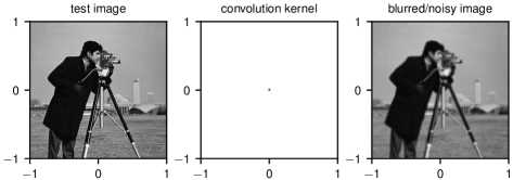
Figure 1: From left to right: ground truth, convolution kernel and noisy image.

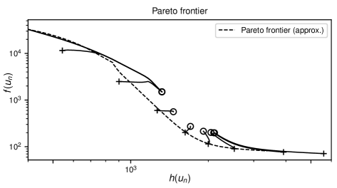
Figure 2: Approximation of the Pareto-frontier by Algorithm (2) in the context of the numerical experiment of Section 5. The dashed line represents the path followed by the iterates of proposed Algorithm (2). The $10$ solid lines, on the other hand, correspond to the paths followed by the classical algorithm (13) for $10$ values of $\mu$ between $10^{3}$ and $10^{-3}$. The circles indicate the positions of the iterates (in the $f-h$ plane) near the start of the iterative process ($n=10$) and the crosses indicate the positions at end of the iterative process ($n=1000$). One sees that the dashed line is indeed a good approximation of the Pareto-frontier for a wide range of the penalty parameter $\mu$, as compared to its samples obtained from running algorithm (13) many times. A logarithmic scale is used on both axes.

6 Conclusions

An optimization-by-continuation algorithm is proposed for problem (1). It is a first order primal-dual method with variable penalty parameters (not variable step lengths). A proof of convergence employing a variable metric criterion was given. Such methods are usually proposed for discussing convergence of Newton-like accelerated first-order optimization algorithms.

Under some additional assumptions on the cost function, the proposed algorithm can be interpreted as a special instance of an inexact proximal algorithm proposed in [11]. It follows that the convergence analysis in [11] is also applicable to the proposed algorithm, however under more restrictive assumptions.

Future work, not addressed in this paper, deals with the convergence of the generalized ISTA algorithm [25, 26] with variable penalty parameters. Another line of research may focus on extending the results here to the more general class of forward backward splitting algorithms, which are suitable for problems formulated in terms of monotone operators without reference to optimization problems [27].

Finally, another topic, also not addressed in this paper, concerns the behavior of the iterates when $N$ penalty parameters $\lambda_{n}$ ($n=1,\ldots,N$) are chosen (e.g. uniformly and decreasing) in a fixed interval $[\lambda_{\min},\lambda_{\max}]$ as is the case in practice. What can be said about the iterates when $N$ tends to infinity? It would indeed be useful to prove that the set of iterates $\{u_{n}^{(N)},n\in[0,N]\}$ approaches the Pareto frontier when $N\to\infty$, or to quantify the distance between those two sets.

References

- [1] A. Chambolle, T. Pock, An introduction to continuous optimization for imaging, Acta Numerica 25 (2016) 161–319. doi:10.1017/S096249291600009X.
- [2] L. Bottou, F. E. Curtis, J. Nocedal, Optimization Methods for Large-Scale Machine Learning, SIAM Review 60 (2) (2018) 223–311. doi:10.1137/16M1080173.
- [3] F. Bach, R. Jenatton, J. Mairal, G. Obozinski, Structured sparsity through convex optimization, Statistical Science 27 (4) (2012). doi:10.1214/12-sts394.
- [4] M. Bertero, P. Boccacci, C. De Mol, Introduction to Inverse Problems in Imaging, Taylor & Francis Group, 2021. doi:10.1201/9781003032755.
- [5] L. Condat, A primal-dual splitting method for convex optimization involving Lipschitzian, proximable and linear composite terms, Journal of Optimization Theory and Applications 158 (2) (2013) 460–479. doi:10.1007/s10957-012-0245-9.
- [6] E. Hale, W. Yin, Y. Zhang, Fixed-point continuation for -minimization: Methodology and convergence, SIAM Journal on Optimization 19 (3) (2008) 1107–1130. doi:10.1137/070698920.
- [7] A. Chambolle, T. Pock, A first-order primal-dual algorithm for convex problems with applications to imaging, Journal of Mathematical Imaging and Vision 40 (1) (2011) 120–145. doi:10.1007/s10851-010-0251-1.
- [8] J.-B. Fest, T. Heikkilä, I. Loris, S. Martin, L. Ratti, S. Rebegoldi, G. Sarnighausen, On a fixed-point continuation method for a convex optimization problem, Springer, 2023, Ch. 25, pp. 100–112, accepted.
- [9] Q.-L. Dong, Y. J. Cho, S. He, P. M. Pardalos, T. M. Rassias, The Krasnosel’skiĭ-Mann Iterative Method, Springer International Publishing, 2022. doi:10.1007/978-3-030-91654-1.
- [10] E. K. Ryu, W. Yin, Large-Scale Convex Optimization, Cambridge University Press, 2022. doi:10.1017/9781009160865.
- [11] J. Rasch, A. Chambolle, Inexact first-order primal-dual algorithms, Computational Optimization and Applications 76 (2) (2020) 381–430. doi:10.1007/s10589-020-00186-y.
- [12] R. T. Rockafellar, Convex Analysis, Princeton University Press, 1970.
- [13] P. L. Combettes, V. R. Wajs, Signal recovery by proximal forward-backward splitting, Multiscale Model. Simul. 4 (4) (2005) 1168–1200. doi:10.1137/050626090.
- [14] J.-J. Moreau, Proximité et dualité dans un espace hilbertien, Bull. Soc. Math. France 93 (1965) 273–299.
- [15] E. van den Berg, M. P. Friedlander, Probing the Pareto frontier for basis pursuit solutions, SIAM Journal on Scientific Computing 31 (2) (2008) 890–912. doi:10.1137/080714488.
- [16] E. van den Berg, M. P. Friedlander, Sparse optimization with least-squares constraints, SIAM Journal on Optimization 21 (4) (2011) 1201–1229. doi:10.1137/100785028.
- [17] S. Boyd, L. Vandenberghe, Convex Optimization, Cambridge University Press, 2004.
- [18] I. Ekeland, R. Temam, Convex Analysis and Variational Problems, Vol. 28 of Classics in Applied Mathematics, SIAM, 1999.
- [19] J.-B. Hiriart-Urruty, C. Lemarechal, Convex analysis and minimization algorithms I: Fundamentals, Springer, 1993.
- [20] B. T. Polyak, Introduction to optimization, Optimization Software, Publications Division, 1987.
- [21] A. Beck, First order methods in optimization, MOS-SIAM Series on Optimization, SIAM, 2017. doi:10.1137/1.9781611974997.
- [22] J.-B. Hiriart-Urruty, C. Lemarechal, Convex analysis and minimization algorithms II: Advanced Theory and Bundle Methods, Springer, 1993.
- [23] S. Salzo, S. Villa, Inexact and accelerated proximal point algorithms, Journal of Convex Analysis 19 (4) (2012) 1167–1192.
- [24] L. I. Rudin, S. Osher, E. Fatemi, Nonlinear total variation based noise removal algorithms, Physica D: Nonlinear Phenomena 60 (1-4) (1992) 259–268. doi:10.1016/0167-2789(92)90242-F.
- [25] I. Loris, C. Verhoeven, On a generalization of the iterative soft-thresholding algorithm for the case of non-separable penalty, Inverse Problems 27 (12) (2011) 125007. doi:10.1088/0266-5611/27/12/125007.
- [26] J. Chen, I. Loris, On starting and stopping criteria for nested primal-dual iterations, Numerical algorithms 82 (2) (2019) 605–621. doi:10.1007/s11075-018-0616-x.
- [27] H. H. Bauschke, P. L. Combettes, Convex Analysis and Monotone Operator Theory in Hilbert Spaces, CMS book in mathematics, Springer, 2011. doi:10.1007/978-1-4419-9467-7.