Using Stochastic Gradient Descent to Smooth Nonconvex Functions:
Analysis of Implicit Graduated Optimization with Optimal Noise Scheduling

Abstract

The graduated optimization approach is a heuristic method for finding globally optimal solutions for nonconvex functions and has been theoretically analyzed in several studies. This paper defines a new family of nonconvex functions for graduated optimization, discusses their sufficient conditions, and provides a convergence analysis of the graduated optimization algorithm for them. It shows that stochastic gradient descent (SGD) with mini-batch stochastic gradients has the effect of smoothing the function, the degree of which is determined by the learning rate and batch size. This finding provides theoretical insights on why large batch sizes fall into sharp local minima, why decaying learning rates and increasing batch sizes are superior to fixed learning rates and batch sizes, and what the optimal learning rate scheduling is. To the best of our knowledge, this is the first paper to provide a theoretical explanation for these aspects. Moreover, a new graduated optimization framework that uses a decaying learning rate and increasing batch size is analyzed and experimental results of image classification that support our theoretical findings are reported.

1 Introduction

1.1 Background

The amazing success of deep neural networks (DNN) in recent years has been based on optimization by stochastic gradient descent (SGD) [57] and its variants, such as Adam [40]. These methods have been widely studied for their convergence [21, 6, 60, 48, 78, 82, 17, 81, 12, 34] and stability [26, 45, 53, 29] in nonconvex optimization.

SGD updates the parameters as $\bm{x}_{t+1}:=\bm{x}_{t}-\eta\nabla f_{\mathcal{S}_{t}}(\bm{x}_{t})$, where $\eta$ is the learning rate and $\nabla f_{\mathcal{S}_{t}}$ is the stochastic gradient estimated from the full gradient $\nabla f$ using a mini-batch $\mathcal{S}_{t}$. Therefore, there is only an $\bm{\omega}_{t}:=\nabla f_{\mathcal{S}_{t}}(\bm{x}_{t})-\nabla f(\bm{x}_{t})$ difference between the search direction of SGD and the true steepest descent direction. This noise is worthless in convex optimization, whereas some studies claim that it is crucial in nonconvex optimization. For example, it has been proven that noise helps the algorithm to escape local minima [23, 37, 18, 27], achieve better generalization [26, 53], and to find a local minimum with a small loss value in polynomial time under some assumptions [79].

[41] also suggests that noise smooths the objective function. Here, at time $t$, let $\bm{y}_{t}$ be the parameter updated by the steepest descent method and $\bm{x}_{t+1}$ be the parameter updated by SGD, i.e.,

$$\bm{y}_{t} :=\bm{x}_{t}-\eta\nabla f(\bm{x}_{t}),$$ (1)

$$\bm{x}_{t+1} :=\bm{x}_{t}-\eta\nabla f_{\mathcal{S}_{t}}(\bm{x}_{t})$$ (2)

$$=\bm{x}_{t}-\eta(\nabla f(\bm{x}_{t})+\bm{\omega}_{t}).$$ (3)

Then, we obtain the following update rule for the sequence $\left\{\bm{y}_{t}\right\}$,

$$\mathbb{E}_{\bm{\omega}_{t}}\left[\bm{y}_{t+1}\right]=\bm{y}_{t}-\eta\nabla\mathbb{E}_{\bm{\omega}_{t}}\left[f(\bm{y}_{t}-\eta\bm{\omega}_{t})\right].$$ (4)

Therefore, if we define a new function $\hat{f}(\bm{y}_{t}):=\mathbb{E}_{\bm{\omega}_{t}}[f(\bm{y}_{t}-\eta\bm{\omega}_{t})]$, $\hat{f}$ can be smoothed by convolving $f$ with noise (see Definition 2.1, also [72]), and its parameters $\bm{y}_{t}$ can approximately be viewed as being updated by using the steepest descent method to minimize $\hat{f}$. In other words, simply using SGD with a mini-batch smooths the function to some extent and may enable escapes from local minima. (The derivation of equation (4) is in Section 6.)

Graduated Optimization. Graduated optimization is one of the global optimization methods, which searches for the global optimal solution of difficult multimodal optimization problems. The method generates a sequence of simplified optimization problems that gradually approach the original problem through different levels of local smoothing operations. Then, it solves the easiest simplified problem first, as it should have nice properties such as convexity or strong convexity; after that, it uses that solution as the initial point for solving the second-simplest problem, then the second solution as the initial point for solving the third-simplest problem and so on, as it attempts to escape from local optimal solutions of the original problem and reach a global optimal solution.

This idea was first established as graduated non-convexity (GNC) by [5] and has since been studied in the field of computer vision for many years. Similar early approaches can be found in [70] and [76], and the same concept appeared in the fields of numerical analysis [1] and optimization [59, 72]. Over the past 25 years, the concept of graduated optimization has been successfully applied to many tasks in computer vision, such as early vision [4], image denoising [54], optical flow [69, 7], dense correspondence of images [39], and robust estimation [73, 2, 55]. In addition, it has been applied to certain tasks in machine learning, such as semi-supervised learning [10, 61, 11], unsupervised learning [62], and ranking [9]. Moreover, score-based generative models [66, 68] and diffusion models [64, 31, 65, 58], which are currently state-of-the-art generative models, implicitly use the techniques of graduated optimization. A comprehensive survey on the graduated optimization approach can be found in [52].

While graduated optimization is popular, there is not much theoretical analysis on it. [51] performed the first theoretical analysis, but they did not provide a practical algorithm. [28] defined a family of nonconvex functions satisfying certain conditions, called $\sigma$-nice, and proposed a first-order algorithm based on graduated optimization. In addition, they studied the convergence and convergence rate of their algorithm to a global optimal solution for $\sigma$-nice functions. [36] proposed a single-loop method that simultaneously updates the variable that defines the noise level and the parameters of the problem and analyzed its convergence. [44] analyzed graduated optimization based on a special smoothing operation.

Figure 1: Conceptual diagram of new $\sigma$-nice function and its smoothed versions (see also the Notation 1).

1.2 Motivation

Equation (4) indicates that SGD smooths the function [41], but it is not clear to what extent the function is smoothed or what factors are involved in the smoothing. Therefore, we decided to clarify these aspects and identify what parameters contribute to the smoothing.

Although [28] proposed a $\sigma$-nice function, it is unclear how special a nonconvex function the $\sigma$-nice function is. In some cases, there may be no function that satisfies the $\sigma$-nice property. We aimed to define and analyze a new family of functions with clear sufficient conditions as replacements for the $\sigma$-nice function.

In graduated optimization, the noise level is gradually reduced, eventually arriving at the original function, but there are an infinite number of ways to reduce the noise. For better optimization, the choice of noise scheduling is a very important issue. Therefore, we also aimed to clarify the optimal noise scheduling theoretically.

Once it is known what parameters of SGD contribute to smoothing and the optimal noise scheduling, an implicit graduated optimization can be achieved by varying the parameters so that the noise level is optimally reduced gradually. Our goal was thus to construct an implicit graduated optimization framework using the smoothing properties of SGD to achieve global optimization of deep neural networks.

1.3 Contributions

SGD’s Smoothing Property. We show that the degree of smoothing by SGD depends on the ratio $\frac{\eta}{\sqrt{b}}$ between the batch size and the learning rate. Accordingly, the smaller the batch size $b$ and the larger the learning rate $\eta$ are, the more smoothed the function becomes (see Figure 1). Also, we can say that halving the learning rate is the same as quadrupling the batch size. Note that [63] makes a somewhat similar claim.

Why the Use of Large Batch Sizes Leads to Solutions Falling into Sharp Local Minima. In other words, from a smoothing perspective, if we use a large batch size and/or a small learning rate, it is easy for the algorithm to fall into a sharp local minimum and experience a drop in generalization performance, since it will optimize a function that is close to the original multimodal function. As is well known, training with a large batch size leads to convergence to sharp local minima and poor generalization performance, as evidenced by the fact that several prior studies [32, 25, 75] provided techniques that do not impair generalization performance even with large batch sizes. [38] showed this experimentally, and our results provide theoretical support for it.

Why Using Decaying Learning Rates and Increasing Batch Sizes is Superior to Using Fixed Ones. Moreover, we can say that decreasing the learning rate and/or increasing the batch size during training is indeed an implicit graduated optimization. Hence, using a decaying learning rate and increasing the batch size makes sense in terms of avoiding local minima. Our results provide theoretical support for the many positive findings on using decaying learning rates [71, 35, 49, 33, 74, 33, 43] and increasing batch sizes [8, 22, 3, 19, 6, 63].

New $\sigma$-nice Function. We propose a new $\sigma$-nice function that generalizes the $\sigma$-nice function. All smoothed functions of the new $\sigma$-nice function are $\sigma$-strongly convex in a neighborhood $B(\bm{x}^{\star};d_{m}|\delta_{m}|)$ of the optimal solution $\bm{x}^{\star}$ that is proportional to the noise level $|\delta_{m}|$ (see Figure 1). In contrast to [41], we show sufficient conditions for a certain nonconvex function $f$ to be a new $\sigma$-nice function as follows:

$$\frac{2\max\left\{\left\|\nabla\hat{f}_{\delta_{m}}(\bm{x}^{\star})\right\|,\left\|\nabla\hat{f}_{\delta_{m+1}}(\bm{x}^{\star})\right\|\right\}}{\sigma\left(1-\gamma_{m}\right)}\leq\left|\delta_{m}\right|=|\delta^{-}|$$ (5)

where $|\delta^{-}|>0,d_{m+1}>1,\gamma_{m}\in\left(\frac{1}{d_{m+1}},1\right)$, and $m\in[M]\subset\mathbb{N}$. $\delta_{m}$ is the noise level of $\hat{f}_{\delta_{m}}$, which is a smoothed version of $f$, and $\bm{x}^{\star}$ is the global optimal solution of the original function $f$. Furthermore, we show that the graduated optimization algorithm for the $L_{f}$-Lipschitz new $\sigma$-nice function converges to an $\epsilon$-neighborhood of the globally optimal solution in $\mathcal{O}\left(1/\epsilon^{\frac{1}{p}+2}\right)\left(p\in(0,1)\right)$ rounds.

Optimal Noise Scheduling. Let $|\delta_{m}|$ be the current noise level, and let the next noise level be determined by $|\delta_{m+1}|:=\gamma_{m}|\delta_{m}|$, where $\gamma_{m}$ is the decay rate of noise. We show theoretically that $\gamma_{m}$ should decay slowly from a value close to 1 for convergence to the globally optimal solution. To the best of our knowledge, ours is the first paper to provide theoretical results on optimal scheduling, both in terms of how to reduce the noise in graduated optimization and how to decay the learning rate and increase the batch size in general optimization. Noise scheduling also has an important role in score-based models [67], diffusion models [15], panoptic segmentation [16], etc., so our theoretical findings will contribute to these methodologies as well.

Furthermore, since the decay rate of noise in graduated optimization is equivalent to the decay rate of the learning rate and rate of increase in batch size, we can say that it is desirable to vary them gradually from a value close to 1. As for the schedule for decaying the learning rate, many previous studies have tried cosine annealing (without restart) [49], cosine power annealing [33], or polynomial decay [47, 14, 80, 13], but it has remained unclear why they are superior to fixed rates. We provide theoretical support showing why they are experimentally superior. In particular, we show that a polynomial decay with a power less than or equal to 1 is the optimal learning rate schedule and demonstrate this in Section 4.

Implicit Graduated Optimization. We propose a new implicit graduated optimization algorithm. The algorithm decreases the learning rate of SGD and increases the batch size during training. We show that the algorithm for the $L_{f}$-Lipschitz new $\sigma$-nice function converges to an $\epsilon$-neighborhood of the globally optimal solution in $\mathcal{O}\left(1/\epsilon^{\frac{1}{p}}\right)\left(p\in(0,1)\right)$ rounds. In Section 4, we show experimentally that methods that reduce noise outperform methods that use a constant learning rate and constant batch size. We also find that methods which increase the batch size outperform those which decrease the learning rate when the decay rate of the noise is set at $1/\sqrt{2}$.

2 Preliminaries

2.1 Definitions and Notation

The notation used in this paper is summarized in Table 1.

Table 1: Notation List

Notation	Description
$\mathbb{N}$	The set of all nonnegative integers
$[N]$	$[N]:=\{1,2,\ldots,N\}$ ($N\in\mathbb{N}\backslash\{0\}$)
$\mathbb{R}^{d}$	A $d$-dimensional Euclidean space with inner product $\langle\cdot,\cdot\rangle$, which induces the norm $\|\cdot\|$
$\mathbb{E}_{\xi}[X]$	The expectation with respect to $\xi$ of a random variable $X$
$\mathcal{S}_{t}$	Mini-batch of $b$ samples $\bm{z}_{i}$ at time $t$
$N(\bm{x}^{\star};\epsilon)$	$\epsilon$-neighborhood of a vector $\bm{x}^{\star}$, i.e., $N(\bm{x}^{\star};\epsilon):=\left\{\bm{x}\in\mathbb{R}^{d}\colon\|\bm{x}-\bm{x}^{\star}\|<\epsilon\right\}$
$B(\bm{x}^{\star};r)$	The Euclidian closed ball of radius $r$ centered at $\bm{x}^{\star}$, i.e., $B(\bm{x}^{\star};r):=\left\{\bm{x}\in\mathbb{R}^{d}\colon\|\bm{x}-\bm{x}^{\star}\|\leq r\right\}$
$\bm{u}\sim B(\bm{x}^{\star};r)$	A random variable distributed uniformly over $B(\bm{x}^{\star};r)$
$M$	The number of smoothed functions, i.e., $M\in\mathbb{N}$
$m$	Counts from the smoothest function, i.e., $m\in[M]$
$\delta$	The degree of smoothing of the smoothed function, i.e., $\delta\in\mathbb{R}$
$\delta_{m}$	The degree of smoothing of the $m$-th smoothed function, i.e., $\delta_{m}\in\mathbb{R}$
$\hat{f}_{\delta}$	The function obtained by smoothing $f$ with a noise level $\delta$
$\hat{f}_{\delta_{m}}$	The $m$-th smoothed function obtained by smoothing $f$ with a noise level $\delta_{m}$
$\bm{x}_{m+1}$	$\bm{x}_{m+1}$ is defined by $\hat{f}_{\delta_{m}}(\bm{x}_{m+1})\leq\hat{f}_{\delta_{m}}(\hat{\bm{x}}_{t})$, where $(\hat{\bm{x}}_{t})_{t=1}^{T_{F}+1}$ is generated by $\text{SGD}(T_{F},\bm{x}_{m},\hat{f}_{\delta_{m}})$
$f_{i}(\bm{x})$	A loss function for $\bm{x}\in\mathbb{R}^{d}$ and $\bm{z}_{i}$
$f(\bm{x})$	The total loss function for $\bm{x}\in\mathbb{R}^{d}$, i.e., $f(\bm{x}):=|\mathcal{S}|^{-1}\sum_{i\in\mathcal{S}}f_{i}(\bm{x})$
$\xi$	A random variable supported on $\Xi$ that does not depend on $\bm{x}\in\mathbb{R}^{d}$
$\xi_{t}$	$\xi_{0},\xi_{1},\ldots$ are independent samples and $\xi_{t}$ is independent of $(\bm{x}_{k})_{k=0}^{t}\subset\mathbb{R}^{d}$
$\xi_{t,i}$	A random variable generated from the $i$-th sampling at time $t$
$\mathsf{G}_{\xi_{t}}(\bm{x})$	The stochastic gradient of $f(\cdot)$ at $\bm{x}\in\mathbb{R}^{d}$
$\nabla f_{\mathcal{S}_{t}}(\bm{x}_{t})$	The mini-batch stochastic gradient of $f(\bm{x}_{t})$ for $\mathcal{S}_{t}$, i.e., $\nabla f_{\mathcal{S}_{t}}(\bm{x}_{t}):=b^{-1}\sum_{i\in[b]}\mathsf{G}_{\xi_{t,i}}(\bm{x}_{t})$

Definition 2.1 (Smoothed function).

Given an $L_{f}$-Lipschitz function $f$, define $\hat{f}_{\delta}$ to be the function obtained by smoothing $f$ as

$$\hat{f}_{\delta}(\bm{x}):=\mathbb{E}_{\bm{u}\sim B(\bm{0};1)}\left[f(\bm{x}-\delta\bm{u})\right],$$ (6)

where $\delta\in\mathbb{R}$ represents the degree of smoothing and $\bm{u}$ is a random variable distributed uniformly over $B(\bm{0};1)$. Also,

$$\bm{x}^{\star}:=\underset{\bm{x}\in\mathbb{R}^{d}}{\operatorname{argmin}}f(\bm{x})\text{\ \ and \ }\bm{x}_{\delta}^{\star}:=\underset{\bm{x}\in\mathbb{R}^{d}}{\operatorname{argmin}}\hat{f}_{\delta}(\bm{x}).$$ (7)

There are a total of $M$ smoothed functions in this paper. The largest noise level is $\delta_{1}$ and the smallest noise level is $\delta_{M+1}=0$. Thus, $\hat{f}_{\delta_{M+1}}=f$.

Definition 2.2 ($\sigma$-nice function [28]).

A function $f\colon\mathbb{R}^{d}\to\mathbb{R}$ is said to be $\sigma$-nice if the following two conditions hold:

(i) For every $\delta>0$ and every $\bm{x}_{\delta}^{\star}$, there exists $\bm{x}_{\delta/2}^{\star}$ such that:

$$\left\|\bm{x}_{\delta}^{\star}-\bm{x}_{\delta/2}^{\star}\right\|\leq\frac{\delta}{2}.$$ (8)

(ii) For every $\delta>0$, let $r_{\delta}=3\delta$; then, the function $\hat{f}_{\delta}(\bm{x})$ over $N(\bm{x}_{\delta}^{\star};r_{\delta})$ is $\sigma$-strongly convex.

2.2 Assumptions and Lemma

We make the following assumptions:

Assumption 2.1.

(A1) $f\colon\mathbb{R}^{d}\to\mathbb{R}$ is continuously differentiable and $L_{g}$-smooth, i.e.,

$$\forall\bm{x},\bm{y}\in\mathbb{R}^{d}:\|\nabla f(\bm{x})-\nabla f(\bm{y})\|\leq L_{g}\|\bm{x}-\bm{y}\|.$$ (9)

(A2) $f\colon\mathbb{R}^{d}\to\mathbb{R}$ is $L_{f}$-Lipschitz function, i.e.,

$$\forall\bm{x},\bm{y}\in\mathbb{R}^{d}:\left|f(\bm{x})-f(\bm{y})\right|\leq L_{f}\|\bm{x}-\bm{y}\|.$$ (10)

(A3) Let $(\bm{x}_{t})_{t\in\mathbb{N}}\subset\mathbb{R}^{d}$ be the sequence generated by an optimizer.

(i) For each iteration $t$,

$$\mathbb{E}_{\xi_{t}}\left[\mathsf{G}_{\xi_{t}}(\bm{x}_{t})\right]=\nabla f(\bm{x}_{t}).$$ (11)

(ii) There exists a nonnegative constant $C^{2}$ such that

$$\mathbb{E}_{\xi_{t}}\left[\|\mathsf{G}_{\xi_{t}}(\bm{x}_{t})-\nabla f(\bm{x}_{t})\|^{2}\right]\leq C^{2}.$$ (12)

(A4) For each iteration $t$, the optimizer samples a mini-batch $\mathcal{S}_{t}\subset\mathcal{S}$ and estimates the full gradient $\nabla f$ as

$$\nabla f_{\mathcal{S}_{t}}(\bm{x}_{t}):=\frac{1}{b}\sum_{i\in[b]}\mathsf{G}_{\xi_{t,i}}(\bm{x}_{t})=\frac{1}{b}\sum_{\{i\colon\bm{z}_{i}\in\mathcal{S}_{t}\}}\nabla f_{i}(\bm{x}_{t}).$$ (13)

Lemma 2.1.

Suppose that (A3)(ii) and (A4) hold for all $t\in\mathbb{N}$; then,

$$\mathbb{E}_{\xi_{t}}\left[\|\nabla f_{\mathcal{S}_{t}}(\bm{x}_{t})-\nabla f(\bm{x}_{t})\|^{2}\right]\leq\frac{C^{2}}{b}.$$

The proof of Lemma 2.1 can be found in Section 7.

3 Main Results

3.1 New $\sigma$-nice function

We generalize the $\sigma$-nice function and define a new $\sigma$-nice function.

Definition 3.1.

A function $f\colon\mathbb{R}^{d}\to\mathbb{R}$ is said to be “new $\sigma$-nice” if the following two conditions hold $\colon$

(i) For all $\delta_{m}\in\mathbb{R}\ (m\in[M])$, and all $\bm{x}_{\delta_{m}}^{\star}$, then

$$\left\|\bm{x}_{\delta_{m}}^{\star}-\bm{x}_{\delta_{m+1}}^{\star}\right\|\leq|\delta_{m}|-|\delta_{m+1}|,$$ (14)

where $|\delta_{m+1}|:=\gamma_{m}|\delta_{m}|\ \left(\gamma_{m}\in\left(\frac{1}{d_{m+1}},1\right)\right)$ (See Proposition 3.1 for the definition of $d_{m}>1$).

(ii) For all $\delta_{m}\in\mathbb{R}\ (m\in[M])$, the function $\hat{f}_{\delta_{m}}(\bm{x})$ is $\sigma$-strongly convex on $N(\bm{x}^{\star};d_{m}\delta_{m})$.

In the definition of the $\sigma$-nice function (Definition 2.2), $\gamma_{m}$ is always $0.5$. We have extended this condition to $\gamma_{m}\in\left(\frac{1}{d_{m+1}},1\right)$. The lower bound on $\gamma_{m}$ is necessary for global convergence of the new $\sigma$-nice function and also provides important insights into the optimal noise scheduling. See Section 3.1.1 for details.

The next propositions provide a sufficient condition for the function $f$ to be a new $\sigma$-nice function. The proofs of Propositions 3.1 and 3.2 are in Section 12.5 and 12.6, respectively.

Proposition 3.1.

Suppose that the function $f\colon\mathbb{R}^{d}\to\mathbb{R}$ is $\sigma$-strongly convex on $B(\bm{x}^{\star};r)$ for sufficiently small $r>0$ and the noise level $|\delta_{m}|$ satisfies $|\delta_{m}|=|\delta^{-}|$; then, the smoothed function $\hat{f}_{\delta_{m}}$ is $\sigma$-strongly convex on $N(\bm{x}^{\star};a_{m}r)\ (a_{m}>\sqrt{2})$, where

$$\begin{split}&|\delta^{-}|:=\Big{|}\|\bm{x}^{\star}-\bm{x}\|\|\bm{u}_{m}\|\cos\theta-\\ &\quad\quad\quad\ \ \sqrt{\|\bm{x}^{\star}-\bm{x}\|^{2}\|\bm{u}_{m}\|^{2}\cos^{2}\theta-r^{2}(a_{m}^{2}-1)}\Big{|},\end{split}$$ (15)

$\bm{x}\in N(\bm{x}^{\star};a_{m}r),\bm{u}_{m}\sim B(\bm{0};1)$, and $\theta$ is the angle between $\bm{u}_{m}$ and $\bm{x}^{\star}-\bm{x}$.

Also, if $d_{m}:=a_{m}r/|\delta^{-}|$ holds, then the smoothed function $\hat{f}_{\delta_{m}}$ is also $\sigma$-strongly convex on $N(\bm{x}^{\star};d_{m}|\delta_{m}|)$.

Now, let us discuss $d_{m}$. From $d_{m}:=a_{m}r/|\delta^{-}|$, the lower and upper bounds of $d_{m}$ can be expressed as

$$1\leq d_{m}\leq\frac{a_{m}}{\sqrt{a_{m}^{2}-1}-1}.$$ (16)

Thus, the upper bound of $d_{m}$ gradually increases as $a_{m}$ decreases. The $\sigma$-nice function [28] always assumes $d_{m}=3$, but we see that this does not hold when $a_{m}$ is large (see Figure 5 in Section 9).

Proposition 3.2.

Suppose that the function $f\colon\mathbb{R}^{d}\to\mathbb{R}$ is $\sigma$-strongly convex on $B(\bm{x}^{\star};r)$ for sufficiently small $r>0$; a sufficient condition for $f$ to be a new $\sigma$-nice function is that the noise level $|\delta_{m}|$ satisfies the following condition $\colon$

For all $m\in[M]$, suppose that $\bm{x}_{\delta_{m}}^{\star}\in N(\bm{x}^{\star};d_{m}|\delta_{m}|)$,

$$\frac{2\max\left\{\left\|\nabla\hat{f}_{\delta_{m}}(\bm{x}^{\star})\right\|,\left\|\nabla\hat{f}_{\delta_{m+1}}(\bm{x}^{\star})\right\|\right\}}{\sigma\left(1-\gamma_{m}\right)}\leq\left|\delta_{m}\right|=\left|\delta^{-}\right|.$$ (17)

Proposition 3.2 shows that any function is a new $\sigma$-nice function if $|\delta_{m}|$ satisfies equations (17). Note that $\delta^{-}$ does not always exist. The probability $p(a_{m})$ that $\delta^{-}$ exists depends on the direction of the random variable vector $\bm{u}_{m}$ and can be expressed as

$$0<p(a_{m}):=\frac{2\arccos\left(\frac{r\sqrt{a_{m}^{2}-1}}{\|\bm{x}^{\star}-\bm{x}\|\|\bm{u}_{m}\|}\right)}{\pi}<1,$$ (18)

where $r>0,a_{m}>\sqrt{2}$, $\bm{x}\in N(\bm{x}^{\star};a_{m}r)$. The probability $p(a_{m})$ approaches $0$ the larger $a_{m}$ is, but never reaches $0$. Therefore, the success of Algorithm 1 depends on the random variable $\bm{u}_{m}$, especially when $a_{m}$ is large, i.e., when $\delta_{m}$ is large.

The framework of graduated optimization for the new $\sigma$-nice function is shown in Algorithm 1. Algorithm 2 is used to optimize each smoothed function.

Algorithm 1 Graduated optimization

0:  $\epsilon>0,r\in(0,1),p\in(0,1),\bar{d}>0,\bm{x}_{1},B_{2}>0$

  $\delta_{1}:=\frac{2L_{f}}{\sigma r}$

  $\alpha_{0}:=\min\left\{\frac{\sigma r}{8L_{f}^{2}\left(1+\bar{d}\right)},\frac{\sqrt{\sigma}r}{2\sqrt{2}L_{f}}\right\},M^{p}:=\frac{1}{\alpha_{0}\epsilon}$

  for $m=1$ to $M+1$ do

     if $m\neq M+1$ then

        $\epsilon_{m}:=\sigma\delta_{m}^{2},\ T_{F}:=2B_{2}/\sigma\epsilon_{m}$

        $\gamma_{m}:=\frac{(M-m)^{p}}{\left\{M-(m-1)\right\}^{p}}$

     end if

     $\bm{x}_{m+1}:=\text{SGD}(T_{F},\bm{x}_{m},\hat{f}_{\delta_{m}})$

     $\delta_{m+1}:=\gamma_{m}\delta_{m}$

  end for

  return  $\bm{x}_{M+2}$

Algorithm 2 SGD with decaying learning rate

0:  $T_{F},\hat{\bm{x}}_{1},F$

  for $t=1$ to $T_{F}$ do

     $\eta_{t}:=2/\sigma t$

     $\hat{\bm{x}}_{t+1}:=\hat{\bm{x}}_{t}-\eta_{t}\nabla F_{\mathcal{S}_{t}}(\hat{\bm{x}}_{t})$

  end for

  return  $\hat{\bm{x}}_{T_{F}+1}=\text{SGD}(T_{F},\hat{\bm{x}}_{1},F)$

The smoothed function $\hat{f}_{\delta_{m}}$ is $\sigma$-strongly convex in the neighborhood $N(\bm{x}^{\star};d_{m}|\delta_{m}|)$. Thus, we should now consider the convergence of SGD for a $\sigma$-strongly convex function $F$. The convergence analysis when using a decaying learning rate is shown in Theorem 3.1 (The proof of Theorem 3.1 is in Section 12.1).

Theorem 3.1 (Convergence analysis of Algorithm 2).

Suppose that (A3) holds, where $\mathsf{G}_{\xi_{t}}$ is the stochastic gradient of a $\sigma$-strongly convex and $L_{g}$-smooth function $F\colon\mathbb{R}^{d}\to\mathbb{R}$, and $\eta_{t}:=\frac{2}{\sigma t}$. Then, the sequence $(\hat{\bm{x}}_{t})_{t\in\mathbb{N}}$ generated by Algorithm 2 satisfies

$$\min_{t\in[T]}\mathbb{E}\left[F\left(\hat{\bm{x}}_{t}\right)-F(\bm{x}^{\star})\right]\leq\frac{2B_{2}}{\sigma T}=\mathcal{O}\left(\frac{1}{T}\right),$$ (19)

where $\bm{x}^{\star}$ is the global minimizer of $F$, and $B_{2}>0$ is a nonnegative constant.

Theorem 3.1 is the convergence analysis of Algorithm 2 for any $\sigma$-strongly convex function $F$. It shows that the algorithm can reach an $\epsilon_{m}$-neighborhood of the optimal solution $\bm{x}_{\delta_{m}}^{\star}$ of $\hat{f}_{\delta_{m}}$ in approximately $T_{F}:=2B_{2}/\sigma\epsilon_{m}$ iterations.

The next theorem guarantees the convergence of Algorithm 1 for the new $\sigma$-nice function (The proof of Theorem 3.2 is in Section 12.2).

Theorem 3.2 (Convergence analysis of Algorithms 1).

Let $\epsilon\in(0,1)$ and $f$ be an $L_{f}$-Lipschitz new $\sigma$-nice function. Suppose that we apply Algorithm 1; then, after $\mathcal{O}\left(1/\epsilon^{\frac{1}{p}+2}\right)$ rounds, the algorithm reaches an $\epsilon$-neighborhood of the global optimal solution $\bm{x}^{\star}$.

3.1.1 Optimal Noise Scheduling

The next proposition is crucial to the success of Algorithm 1 (The proof is in Section 12.7).

Proposition 3.3.

Suppose that $f\colon\mathbb{R}^{d}\to\mathbb{R}$ is a new $\sigma$-nice function. Then,

$$\forall m\in[M-1]\colon\left\|\bm{x}_{\delta_{m}}^{\star}-\bm{x}^{\star}\right\|<d_{m+1}|\delta_{m+1}|.$$ (20)

Assuming that Algorithm 2 comes sufficiently close to the optimal solution $\bm{x}_{\delta_{m}}^{\star}$ after more than $T_{F}$ iterations in the optimization of the $\hat{f}_{\delta_{m}}$, $\bm{x}_{\delta_{m}}^{\star}$ is the initial point of the optimization of the next function $\hat{f}_{\delta_{m+1}}$. Proposition 3.3 therefore implies that the initial point of optimization of the function $\hat{f}_{\delta_{m}}$ is contained in the $\sigma$-strongly convex region of the next function $\hat{f}_{\delta_{m+1}}$. This means that if the initial point $\bar{\bm{x}}_{1}$ of Algorithm 1 is contained in the $\sigma$-strongly convex region $N(\bm{x}^{\star};d_{1}|\delta_{1}|)$ of the smoothest function $\hat{f}_{\delta_{1}}$, then the algorithm will always reach the globally optimal solution $\bm{x}^{\star}$ of the original function $f$.

For Proposition 3.3 to hold, $\gamma_{m}\in\left(\frac{1}{d_{m+1}},1\right)$ must also hold (The proof of this claim is in Section 12.7). Now, let us discuss $1/d_{m}$. From $d_{m}:=a_{m}r/|\delta^{-}|$, the lower and upper bounds of $1/d_{m}$ can be expressed as

$$\frac{\sqrt{a_{m}^{2}-1}-1}{a_{m}}\leq\frac{1}{d_{m}}\leq 1.$$ (21)

Thus, the lower bound of the decay rate $\gamma_{m}$ decreases gradually as $a_{m}$ decreases. For convergence to the globally optimal solution, the noise decay rate should be decreased slowly from a value close to $1$ (see Figure 5 in Section 9). A more detailed discussion of optimal noise scheduling is presented in Section 9.

3.2 SGD’s smoothing property

This section discusses the smoothing effect of using stochastic gradients. From Lemma 2.1, we have

$$\mathbb{E}_{\xi_{t}}\left[\left\|\bm{\omega}_{t}\right\|\right]\leq\frac{C}{\sqrt{b}},$$ (22)

due to $\bm{\omega}_{t}:=\nabla f_{\mathcal{S}_{t}}(\bm{x}_{t})-\nabla f(\bm{x}_{t})$. The $\bm{\omega}_{t}$ for which this equation is satisfied can be expressed as $\bm{\omega}_{t}=\frac{C}{\sqrt{b}}\bm{u}_{t}\ (\bm{u}_{t}\sim B(\bm{0};1))$. Then, using Definition 2.1, we further transform equation (4) as follows:

$$\mathbb{E}_{\bm{\omega}_{t}}\left[\bm{y}_{t+1}\right] =\bm{y}_{t}-\eta\nabla\mathbb{E}_{\bm{\omega}_{t}}\left[f(\bm{y}_{t}-\eta\bm{\omega}_{t})\right]$$ (23)

$$=\bm{y}_{t}-\eta\nabla\mathbb{E}_{\bm{u}_{t}\sim B(\bm{0};1)}\left[f\left(\bm{y}_{t}-\frac{\eta C}{\sqrt{b}}\bm{u}_{t}\right)\right]$$ (24)

$$=\bm{y}_{t}-\eta\nabla\hat{f}_{\frac{\eta C}{\sqrt{b}}}(\bm{y}_{t}).$$ (25)

This shows that $\mathbb{E}_{\bm{\omega}_{t}}\left[f(\bm{y}_{t}-\eta\bm{\omega}_{t})\right]$ is a smoothed version of $f$ with a noise level $\eta C/\sqrt{b}$ and its parameter $\bm{y}_{t}$ can be approximately updated by using the steepest descent method to minimize $\hat{f}_{\frac{\eta C}{\sqrt{b}}}$. Therefore, we can say that the degree of smoothing by the stochastic gradients in SGD is determined by the learning rate $\eta$ and batch size $b$. The findings gained from this insight are immeasurable.

3.2.1 Why the Use of Large Batch Sizes Leads to Solutions Falling into Sharp Local Minima

It is known that training with large batch sizes leads to a persistent degradation of model generalization performance. In particular, [38] showed experimentally that learning with large batch sizes leads to sharp local minima and worsens generalization performance. According to equation (25), using a large learning rate and/or a small batch size will make the function smoother. Thus, in using a small batch size, the sharp local minima will disappear through extensive smoothing, and SGD can reach a flat local minimum. Conversely, when using a large batch size, the smoothing is weak and the function is close to the original multimodal function, so it is easy for the solution to fall into a sharp local minimum. Thus, we have theoretical support for what [38] showed experimentally. In addition, equation (25) implies that halving the learning rate is the same as quadrupling the batch size. Note that [63] argues that reducing the learning rate by half is equivalent to doubling the batch size.

3.2.2 Why Decaying Learning Rates and Increasing Batch Sizes are Superior to Fixed Learning Rates and Batch Sizes

From equation (23), the use of a decaying learning rate or increasing batch size during training is equivalent to decreasing the noise level of the smoothed function, so using a decaying learning rate or increasing the batch size is an implicit graduated optimization. Thus, we can say that using a decaying learning rate [49, 33, 74, 43] or increasing batch size [8, 22, 3, 19, 6, 63] makes sense in terms of avoiding local minima and provides theoretical support for their experimental superiority.

3.2.3 Optimal Decay Rate of Learning Rate

As indicated in Section 3.1.1, gradually decreasing the noise from a value close to 1 is an optimal noise scheduling for graduated optimization. Therefore, we can say that the optimal update rule for a decaying learning rate and increasing batch size is varying slowly from a value close to 1, as in cosine annealing (without restart) [49], cosine power annealing [33], and polynomial decay [47, 14, 80, 13]. Thus, we have a theoretical explanation for why these schedules are superior. In particular, a polynomial decay with small powers from 0 to 1 satisfies the conditions that the decay rate must satisfy (see also Figures 6 and 8 in Section 9). Therefore, we argue that polynomial decays with powers less than equal to 1 are the optimal decaying learning rate schedule.

3.3 Implicit graduated optimization algorithm

Algorithm 3 embodies the framework of implicit graduated optimization for the new $\sigma$-nice function. Algorithm 4 is used to optimize each smoothed function. The $\gamma_{m}$ used in Algorithms 1 and 3 is a polynomial decay rate with powers from 0 to 1. The smoothed function $\hat{f}_{\delta_{m}}$ is $\sigma$-strongly convex in the neighborhood $N(\bm{x}^{\star};d_{m}|\delta_{m}|)$. Also, the learning rate used by Algorithm 4 to optimize $\hat{f}_{\delta_{m}}$ is always constant. Therefore, let us now consider the convergence of SGD with a constant learning rate for a $\sigma$-strongly convex function $F$. The proof of Theorem 3.3 is in Section 12.3.

Theorem 3.3 (Convergence analysis of Algorithm 4).

Suppose that (A3) holds, where $\mathsf{G}_{\xi_{t}}$ is the stochastic gradient of a $\sigma$-strongly convex and $L_{g}$-smooth function $F\colon\mathbb{R}^{d}\to\mathbb{R}$, and $\eta<\min\left\{\frac{1}{\sigma},\frac{2}{L_{g}}\right\}$. Then, the sequence $(\hat{\bm{x}}_{t})_{t\in\mathbb{N}}$ generated by Algorithm 4 satisfies

$$\min_{t\in[T]}\mathbb{E}\left[F\left(\hat{\bm{x}}_{t}\right)-F(\bm{x}^{\star})\right]\leq\frac{H_{4}}{T}+H_{3}\eta=\mathcal{O}\left(\frac{1}{T}+\eta\right),$$ (26)

where $\bm{x}^{\star}$ is the global minimizer of $F$, and $H_{4}\text{ and }H_{3}>0$ are nonnegative constants.

Theorem 3.3 is the convergence analysis of Algorithm 4 for any $\sigma$-strongly convex and $L_{g}$-smooth function $F$. It shows that Algorithm 4 can reach an $\epsilon_{m}$-neighborhood of the optimal solution $\bm{x}_{\delta_{m}}^{\star}$ of $\hat{f}_{\delta_{m}}$ in approximately $T_{F}:=H_{4}/\left(\epsilon_{m}-H_{3}\eta\right)$ iterations. Since Proposition 3.3 holds for any $\delta\in\mathbb{R}$, it also holds for Algorithm 3. Therefore, if the initial point $\bar{\bm{x}}_{1}$ is contained in the $\sigma$-strongly convex region $N(\bm{x}^{\star};d_{1}|\delta_{1}|)$ of the smoothest function $\hat{f}_{\delta_{1}}$, then the algorithm will always reach the globally optimal solution $\bm{x}^{\star}$ of the original function $f$.

Algorithm 3 Implicit Graduated Optimization

0:  $\epsilon>0,p\in(0,1),\bar{d}>0,\bm{x}_{1},\eta_{1},b_{1}$

  $\delta_{1}:=\frac{\eta_{1}C}{\sqrt{b_{1}}}$

  $\alpha_{0}:=\min\left\{\frac{\sqrt{b_{1}}}{4L_{f}\eta_{1}C\left(1+\bar{d}\right)},\frac{\sqrt{b_{1}}}{\sqrt{2\sigma}\eta_{1}C}\right\},M^{p}:=\frac{1}{\alpha_{0}\epsilon}$

  for $m=1$ to $M+1$ do

     if $m\neq M+1$ then

        $\epsilon_{m}:=\sigma^{2}\delta_{m}^{2},\ T_{F}:=H_{4}/\left(\epsilon_{m}-H_{3}\eta_{m}\right)$

        $\gamma_{m}:=\frac{(M-m)^{p}}{\left\{M-(m-1)\right\}^{p}}$

        $\kappa_{m}/\sqrt{\lambda_{m}}=\gamma_{m}\ (\kappa_{m}\in(0,1],\lambda_{m}\geq 1)$

     end if

     $\bm{x}_{m+1}:=\text{SGD}(T_{F},\bm{x}_{m},\hat{f}_{\delta_{m}},\eta_{m},b_{m})$

     $\eta_{m+1}:=\kappa_{m}\eta_{m},b_{m+1}:=\lambda_{m}b_{m}$

     $\delta_{m+1}:=\frac{\eta_{m+1}C}{\sqrt{b_{m+1}}}$

  end for

  return  $\bm{x}_{M+2}$

Algorithm 4 SGD with a constant learning rate

0:  $T_{F},\hat{\bm{x}}_{1},F,\eta,b$

  for $t=1$ to $T_{F}$ do

     $\hat{\bm{x}}_{t+1}:=\hat{\bm{x}}_{t}-\eta\nabla F_{\mathcal{S}_{t}}(\bm{x}_{t})$

  end for

  return  $\hat{\bm{x}}_{T_{F}+1}=\text{SGD}(T_{F},\hat{\bm{x}}_{1},F,\eta,b)$

The next theorem guarantees the convergence of Algorithm 3 with the new $\sigma$-nice function (The proof of Theorem 3.4 is in Section 12.4).

Theorem 3.4.

[Convergence analysis of Algorithm 3] Let $\epsilon\in(0,1)$ and $f$ be an $L_{f}$-Lipschitz new $\sigma$-nice function. Suppose that we apply Algorithm 3; then after $\mathcal{O}\left(1/\epsilon^{\frac{1}{p}}\right)$ rounds, the algorithm reaches an $\epsilon$-neighborhood of the global optimal solution $\bm{x}^{\star}$.

4 Numerical Results

4.1 Implicit Graduated Optimization of DNN

We compared four types of SGD for image classification:

1. constant learning rate and constant batch size,

2. decaying learning rate and constant batch size,

3. constant learning rate and increasing batch size,

4. decaying learning rate and increasing batch size.

All experiments were run for 200 epochs with a noise decay of $1/\sqrt{2}$ every 40 epochs. That is, every 40 epochs, the learning rate of method 2 was multiplied by $1/\sqrt{2}$, the batch size of method 3 was doubled, and the learning rate and batch size of method 4 were respectively multiplied by $\sqrt{3}/2$ and $1.5$.

We evaluated the performance of the four SGDs in training WideResNet-28-10 [77] on CIFAR100 dataset [42]. Figure 2 plots the accuracy in testing and the loss function value in training versus epochs. We also evaluated the performance of the four SGDs in training ResNet18 [30] on CIFAR100 dataset and ResNet34 [30] on ImageNet dataset [20] and obtained similar results (see Figures 9 and 11 in Section 10.1).

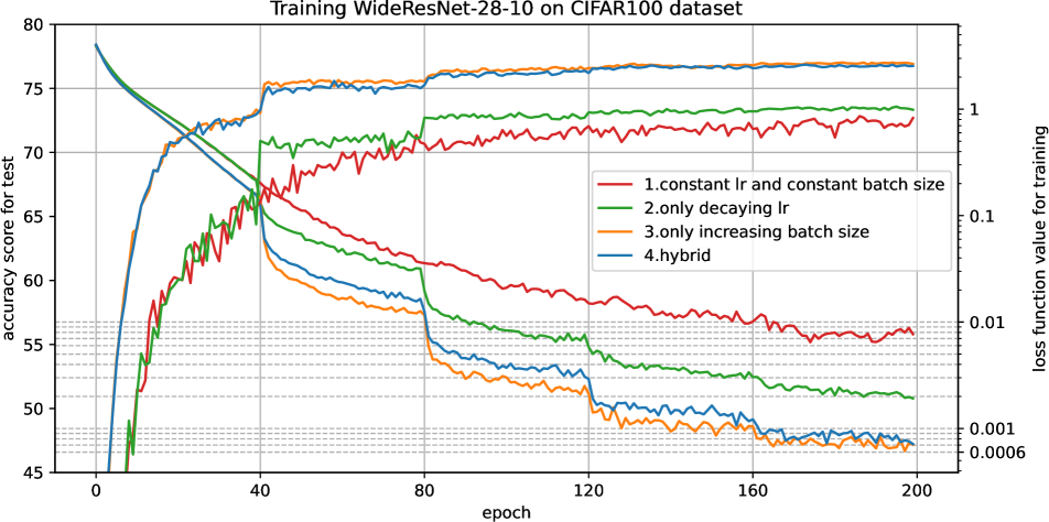
Figure 2: Accuracy score for testing and loss function value for training versus epochs in training of WideResNet-28-10 on CIFAR100 dataset. The average of multiple runs is plotted.

When the decay rate of the noise was set at $1/\sqrt{2}$, the method that decreases the learning rate and increases the batch size and the method that only increases batch size had superior accuracy and lower training loss function values compared with the one that only decays the learning rate in all of the experiments. In theory, decreasing the learning rate and increasing the batch size are equivalent in terms of reducing the noise in the smoothed function, but in the experiments, the SGD that only decreased the learning rate was not equivalent to the one that only increased the batch size because the frequency of parameter updates changed as the batch size was increased. Therefore, an increasing batch size is more effective than a decaying learning rate, which is also consistent with the claim in [63]. The three noise reducing methods also outperform the methods using a constant learning rate and constant batch size in terms of accuracy in testing. Thus, we can say that the implicit graduated optimization algorithm works well and reaches a better local solution with superior generalizability.

4.2 Experiments on Optimal Noise Scheduling

Section 3.2.3 shows that the optimal decaying learning rate is in theory a polynomial decay with small powers from 0 to 1. To demonstrate this, we evaluated the performance of SGDs with several decaying learning rate schedules in training ResNet18 on CIFAR100 dataset. Figure 3 plots the accuracy in testing and the loss function value in training versus epochs. We also evaluated the performance of SGDs with several decaying learning rate schedules in training WideResNet-28-10 on CIFAR100 dataset and obtained similar results (see Figure 13 in Section 10.2). The batch size was fixed at 128 in all runs.

Figure 3: Accuracy score for testing and loss function value for training versus epochs in training of ResNet18 on CIFAR100 dataset. The average of multiple runs is plotted.

Figure 3 shows that a polynomial decay with powers as small as from 0 to 1 can achieve lower loss function values in training and higher accuracy scores in testing than polynomial decay with powers greater than 1, cosine annealing, and exponential decay [71]. This is completely consistent with theory (see also Figures 6 and 8 in Section 9).

5 Conclusion

We defined a family of nonconvex functions: new $\sigma$-nice functions that prove that the graduated optimization approach converges to a globally optimal solution. We also provided sufficient conditions for any nonconvex function to be a new $\sigma$-nice function and performed a convergence analysis of the graduated optimization algorithm for the new $\sigma$-nice functions. We proved that SGD with a mini-batch stochastic gradient has the effect of smoothing the function, and the degree of smoothing is greater with larger learning rates and smaller batch sizes. This shows theoretically that smoothing with large batch sizes is makes it easy to fall into sharp local minima, that using a decaying learning rate and/or increasing batch size is implicitly graduated optimization, which makes sense in the sense that it avoids local solutions, and that the optimal learning rate scheduling rule is a gradual scheduling with a decreasing rate, such as a polynomial decay with small powers. Based on these findings, we proposed a new graduated optimization algorithm that uses a decaying learning rate and increasing batch size and analyzed it. Finally, we conducted experiments whose results showed the superiority of our recommended framework for image classification tasks on CIFAR100 and ImageNet and that polynomial decay with small powers is an optimal decaying learning rate schedule.

6 Derivation of equation (4)

Let $\bm{y}_{t}$ be the parameter updated by the steepest descent method and $\bm{x}_{t+1}$ be the parameter updated by SGD at time $t$, i.e.,

$$\bm{y}_{t} :=\bm{x}_{t}-\eta\nabla f(\bm{x}_{t}),$$ (27)

$$\bm{x}_{t+1} :=\bm{x}_{t}-\eta\nabla f_{\mathcal{S}_{t}}(\bm{x}_{t})$$ (28)

$$=\bm{x}_{t}-\eta(\nabla f(\bm{x}_{t})+\bm{\omega}_{t}).$$ (29)

Then, we have

$$\bm{x}_{t+1} :=\bm{x}_{t}-\eta\nabla f_{\mathcal{S}_{t}}(\bm{x}_{t})$$ (30)

$$=\left(\bm{y}_{t}+\eta\nabla f(\bm{x}_{t})\right)-\eta\nabla f_{\mathcal{S}_{t}}(\bm{x}_{t})$$ (31)

$$=\bm{y}_{t}-\eta\bm{\omega}_{t},$$ (32)

from $\bm{\omega}_{t}:=\nabla f_{\mathcal{S}_{t}}(\bm{x}_{t})-\nabla f(\bm{x}_{t})$. Hence,

$$\bm{y}_{t+1} =\bm{x}_{t+1}-\eta\nabla f(\bm{x}_{t+1})$$ (33)

$$=\bm{y}_{t}-\eta\bm{\omega}_{t}-\eta\nabla f(\bm{y}_{t}-\eta\bm{\omega}_{t}).$$ (34)

By taking the expectation with respect to $\bm{\omega}_{t}$ on both sides, we have, from $\mathbb{E}_{\bm{\omega}_{t}}\left[\bm{\omega}_{t}\right]=\bm{0}$,

$$\mathbb{E}_{\bm{\omega}_{t}}\left[\bm{y}_{t+1}\right]=\bm{y}_{t}-\eta\nabla\mathbb{E}_{\bm{\omega}_{t}}\left[f(\bm{y}_{t}-\eta\bm{\omega}_{t})\right].$$ (35)

In addition, from (32) and $\mathbb{E}_{\bm{\omega}_{t}}\left[\bm{\omega}_{t}\right]=\bm{0}$, we obtain

$$\mathbb{E}_{\bm{\omega}_{t}}\left[\bm{x}_{t+1}\right]=\bm{y}_{t}.$$ (36)

Therefore, on average, the parameter $\bm{x}_{t+1}$ of the function $f$ arrived at by SGD coincides with the parameter $\bm{y}_{t}$ of the smoothed function $\hat{f}(\bm{y}_{t}):=\nabla\mathbb{E}_{\bm{\omega}_{t}}\left[f(\bm{y}_{t}-\eta\bm{\omega}_{t})\right]$ arrived at by the steepest descent method.

7 Proof of Lemma 2.1

Proof.

(A3)(ii) and (A4) guarantee that

$$\mathbb{E}\left[\|\nabla f_{\mathcal{S}_{t}}(\bm{x}_{t})-\nabla f(\bm{x}_{t})\|^{2}\right] =\mathbb{E}\left[\left\|\frac{1}{b}\sum_{i=1}^{b}{\mathsf{G}_{\xi_{t,i}}(\bm{x}_{t})}-\nabla f(\bm{x}_{t})\right\|^{2}\right]$$ (37)

$$=\mathbb{E}\left[\left\|\frac{1}{b}\sum_{i=1}^{b}{\mathsf{G}_{\xi_{t,i}}(\bm{x}_{t})}-\frac{1}{b}\sum_{i=1}^{b}\nabla f(\bm{x}_{t})\right\|^{2}\right]$$ (38)

$$=\mathbb{E}\left[\left\|\frac{1}{b}\sum_{i=1}^{b}\left({\mathsf{G}_{\xi_{t,i}}(\bm{x}_{t})-\nabla f(\bm{x}_{t})}\right)\right\|^{2}\right]$$ (39)

$$=\frac{1}{b^{2}}\mathbb{E}\left[\left\|\sum_{i=1}^{b}\left({\mathsf{G}_{\xi_{t,i}}(\bm{x}_{t})-\nabla f(\bm{x}_{t})}\right)\right\|^{2}\right]$$ (40)

$$=\frac{1}{b^{2}}\mathbb{E}\left[\sum_{i=1}^{b}\left\|{\mathsf{G}_{\xi_{t,i}}(\bm{x}_{t})-\nabla f(\bm{x}_{t})}\right\|^{2}\right]$$ (41)

$$\leq\frac{C^{2}}{b}.$$ (42)

This completes the proof. ∎

8 Discussion on smoothed functions

Lemma 8.1.

Suppose that (A1) holds; then, $\hat{f}_{\delta}$ defined by (6) is also $L_{g}$-smooth; i.e., for all $\bm{x},\bm{y}\in\mathbb{R}^{d}$,

$$\left\|\nabla\hat{f}_{\delta}(\bm{x})-\nabla\hat{f}_{\delta}(\bm{y})\right\|\leq L_{g}\|\bm{x}-\bm{y}\|.$$ (43)

Proof.

From Definition 2.1 and (A1), we have, for all $\bm{x},\bm{y}\in\mathbb{R}^{d}$,

$$\left\|\nabla\hat{f}_{\delta}(\bm{x})-\nabla\hat{f}_{\delta}(\bm{y})\right\| =\left\|\nabla\mathbb{E}_{\bm{u}}\left[f(\bm{x}-\delta\bm{u})\right]-\nabla\mathbb{E}_{\bm{u}}\left[f(\bm{y}-\delta\bm{u})\right]\right\|$$ (44)

$$=\left\|\mathbb{E}_{\bm{u}}\left[\nabla f(\bm{x}-\delta\bm{u})\right]-\mathbb{E}_{\bm{u}}\left[\nabla f(\bm{y}-\delta\bm{u})\right]\right\|$$ (45)

$$=\left\|\mathbb{E}_{\bm{u}}\left[\nabla f(\bm{x}-\delta\bm{u})-\nabla f(\bm{y}-\delta\bm{u})\right]\right\|$$ (46)

$$\leq\mathbb{E}_{\bm{u}}\left[\left\|\nabla f(\bm{x}-\delta\bm{u})-\nabla f(\bm{y}-\delta\bm{u})\right\|\right]$$ (47)

$$\leq\mathbb{E}_{\bm{u}}\left[L_{g}\left\|(\bm{x}-\delta\bm{u})-(\bm{y}-\delta\bm{u})\right\|\right]$$ (48)

$$=\mathbb{E}_{\bm{u}}\left[L_{g}\left\|\bm{x}-\bm{y}\right\|\right]$$ (49)

$$=L_{g}\|\bm{x}-\bm{y}\|.$$ (50)

This completes the proof. ∎

Lemma 8.2.

Suppose that (A2) holds; then $\hat{f}_{\delta}$ is also an $L_{f}$-Lipschitz function; i.e., for all $\bm{x},\bm{y}\in\mathbb{R}^{d}$,

$$\left|\hat{f}_{\delta}(\bm{x})-\hat{f}_{\delta}(\bm{y})\right|\leq L_{f}\|\bm{x}-\bm{y}\|.$$ (51)

Proof.

From Definition 2.1 and (A2), we have, for all $\bm{x},\bm{y}\in\mathbb{R}^{d}$,

$$\left|\hat{f}_{\delta}(\bm{x})-\hat{f}_{\delta}(\bm{y})\right| =\left|\mathbb{E}_{\bm{u}}\left[f(\bm{x}-\delta\bm{u})\right]-\mathbb{E}_{\bm{u}}\left[f(\bm{y}-\delta\bm{u})\right]\right|$$ (52)

$$=\left|\mathbb{E}_{\bm{u}}\left[f(\bm{x}-\delta\bm{u})-f(\bm{y}-\delta\bm{u})\right]\right|$$ (53)

$$\leq\mathbb{E}_{\bm{u}}\left[\left|f(\bm{x}-\delta\bm{u})-f(\bm{y}-\delta\bm{u})\right|\right]$$ (54)

$$\leq\mathbb{E}_{\bm{u}}\left[L_{f}\|(\bm{x}-\delta\bm{u})-(\bm{y}-\delta\bm{u})\|\right]$$ (55)

$$=\mathbb{E}_{\bm{u}}\left[L_{f}\left\|\bm{x}-\bm{y}\right\|\right]$$ (56)

$$=L_{f}\|\bm{x}-\bm{y}\|.$$ (57)

This completes the proof. ∎

Lemmas 8.1 and 8.2 imply that the Lipschitz constants $L_{f}$ of the original function $f$ and $L_{g}$ of $\nabla f$ are taken over by the smoothed function $\hat{f}_{\delta}$ and its gradient $\nabla\hat{f}_{\delta}$ for all $\delta\in\mathbb{R}$.

Lemma 8.3.

Let $\hat{f}_{\delta}$ be the smoothed version of $f$; then, for all $\bm{x}\in\mathbb{R}^{d}$,

$$\left|\hat{f}_{\delta}(\bm{x})-f(\bm{x})\right|\leq|\delta|L_{f}.$$ (58)

Proof.

From Definition 2.1 and (A2), we have, for all $\bm{x},\bm{y}\in\mathbb{R}^{d}$,

$$\left|\hat{f}_{\delta}(\bm{x})-f(\bm{x})\right| =\left|\mathbb{E}_{\bm{u}}\left[f(\bm{x}-\delta\bm{u})\right]-f(\bm{x})\right|$$ (59)

$$=\left|\mathbb{E}_{\bm{u}}\left[f(\bm{x}-\delta\bm{u})-f(\bm{x})\right]\right|$$ (60)

$$\leq\mathbb{E}_{\bm{u}}\left[\left|f(\bm{x}-\delta\bm{u})-f(\bm{x})\right|\right]$$ (61)

$$\leq\mathbb{E}_{\bm{u}}\left[L_{f}\|(\bm{x}-\delta\bm{u})-\bm{x}\|\right]$$ (62)

$$=\mathbb{E}_{\bm{u}}\left[L_{f}|\delta|\|\bm{u}\|\right]$$ (63)

$$=|\delta|L_{f},$$ (64)

where we have used $\|\bm{u}\|\leq 1$. This completes the proof. ∎

Lemma 8.3 implies that the larger the degree of smoothing is, the further away the smoothed function is from the original function. Since the degree of smoothing is determined by the learning rate and batch size (see Section 3.2), we can say that the optimal value obtained by using a large learning rate and/or small batch size may be larger than the optimal value obtained by using a small learning rate and/or large batch size. When decreasing the learning rate or increasing the batch size, the sharp decrease in function values at that time depends on a change of the objective function (see also Figure 1), and this phenomenon is especially noticeable in schedules that use the same noise level for multiple epochs, such as step decay learning rate (see Figures 9-11).

9 Discussion on optimal noise scheduling

According to Proposition 3.1, for a function to be a new $\sigma$-nice function, $d_{m}$ must satisfy equation (16). Thus, there is a range of possible values for $1/d_{m}$, as shown in equation (21). Equation (16) and (21) are restated below,

$$1\leq d_{m}\leq\frac{a_{m}}{\sqrt{a_{m}^{2}-1}-1}\text{\ and }\frac{\sqrt{a_{m}^{2}-1}-1}{a_{m}}\leq\frac{1}{d_{m}}\leq 1,$$ (65)

and their range is plotted in Figure 5. Recall that $a_{m}$ is a value that appears only in the theoretical analysis and it becomes smaller as $m$ increases and $\delta_{m}$ decreases, since it satisfies $d|\delta_{m}|=a_{m}r$.

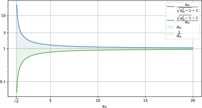
Figure 4: The range of possible values for $d_{m}$ and $1/d_{m}$ are filled in blue and green, respectively. Note that the vertical axis is logarithmic.

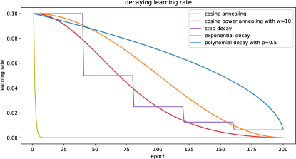
Figure 5: Existing decay learning rate versus number of epochs. The schedule definitions are included in equations (66) through (70).

$d_{m}$ is involved in the radius of the strongly convex region $N(\bm{x}^{\star};d_{m}|\delta_{m}|)$ of the smoothed function $\hat{f}_{\delta_{m}}$. According to Figure 5, when $a_{m}$ is large, i.e., when $m$ is small and $|\delta_{m}|$ is large, $d_{m}$ can only take almost 1. By definition of a $\sigma$-nice function [28] (see Definition 2.2), a smoothed function $\hat{f}_{\delta_{m}}$ is strongly convex in a neighborhood $N(\bm{x}_{\delta_{m}}^{\star};3\delta_{m})$. Then, if $\bm{x}_{\delta_{m}}^{\star}$ is contained in $N(\bm{x}^{\star};d_{m}\delta_{m})$, we see that $d_{m}=3$ does not always hold.

From Proposition 3.3 and its proof, for Algorithm 1 to be successful, $1/d_{m+1}$ is required as a lower bound for $\gamma_{m}$, i.e., $\gamma_{m}\in\left(\frac{1}{d_{m+1}},1\right)$. Recall that $\gamma_{m}$ is the decay rate of the noise level $|\delta_{m}|$, i.e., $|\delta_{m+1}|:=\gamma_{m}|\delta_{m}|$. According to Figure 5, when $a_{m}$ is large, i.e., when $m$ is small and $|\delta_{m}|$ is large, $1/d_{m}$ and $\gamma_{m}$ can only take almost 1. Therefore, $\gamma_{m}$ should vary very gradually from a value close to 1. Once the optimal $\left(\gamma_{m}\right)_{m\in[M]}$ is determined, the optimal $\left(\delta_{m}\right)_{m\in[M]}$ is also determined.

Now let us see if there exists a decaying learning rate schedule that satisfies the decay rate $\gamma_{m}$ condition. The existing decaying learning rate schedule is shown in Figure 5 (Methods that include an increase in the learning rate, even partially, such as warm-up, are omitted). The following defines the update rules for all decaying learning rates $(\eta_{t})_{t\in\left\{0,1,\cdots,T-1\right\}}$, where $T$ means the number of epochs.

cosine annealing [49]: $$\eta_{t}:=\eta_{\min}+\frac{1}{2}\left(\eta_{\max}-\eta_{\min}\right)\left(1+\cos\left(\frac{t}{T}\pi\right)\right)$$ (66)

cosine power annealing [33]: $$\eta_{t}:=\eta_{\min}+\left(\eta_{\max}-\eta_{\min}\right)\frac{w^{\frac{1}{2}\left(1+\cos\left(\frac{t}{T}\pi\right)\right)+1}-w}{w^{2}-w}\ \ (w>0)$$ (67)

step decay [50]: $$\eta_{t}:=\eta_{\max}d^{\lfloor\frac{t}{n}\rfloor}\ (0<d<1,n<T)$$ (68)

exponential decay [71]: $$\eta_{t}:=\eta_{\max}\exp\left(-kt\right)\ (k>0)$$ (69)

polynomial decay [14]: $$\eta_{t}:=\left(\eta_{\max}-\eta_{\min}\right)\left(1-\frac{t}{T}\right)^{p}+\eta_{\min}\ (p>0)$$ (70)

The curves in Figure 5 are plotted for $T=200,\eta_{\min}=0,\eta_{\max}=0.1,d=0.5,n=40,k=0.94,w=10$ and $p=0.5$. The decay rates of these schedules are plotted in Figure 6. Figure 8 and Figure 8 are for polynomial decays with different parameters $p$. Note that $\eta_{\min}$ is 0, but since $t\in[0,1,\cdots,T-1]$, $\eta_{t}$ will never be 0 under any update rule. In Figure 6 and 8, only the first one is set to 1 artificially. Also, the value shown at epoch $t$ represents the rate of decay from the learning rate used in epoch $t$ to the learning rate used in epoch $t+1$. Therefore, the graphs stops at 199 epochs.

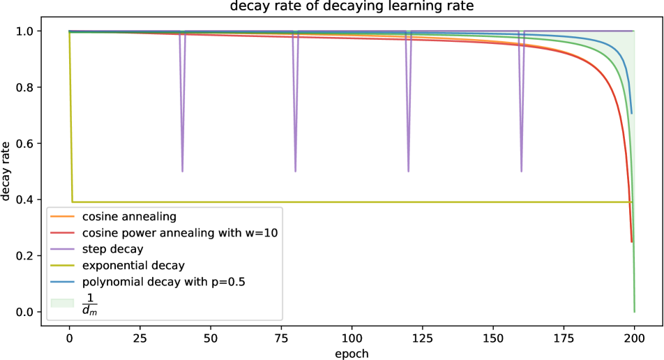
Figure 6: Decay rate of the existing decaying learning rate schedule. The area filled in green represents the value that the decay rate $\gamma_{m}$ must satisfy for the graduated optimization approach to succeed. Here, the green curve in this figure is a symmetric shift and parallel shift of the green curve in Figure 5 to zero at epoch 200.

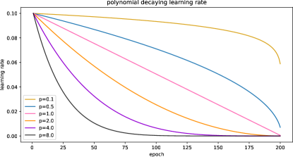
Figure 7: Polynomial decay learning rate versus epoch. The update rule for polynomial decay is defined by (70).

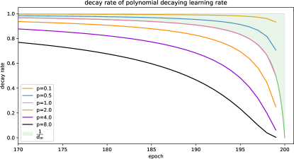
Figure 8: Decay rate of polynomial decay learning rate schedule. The area filled in green represents the value that the decay rate $\gamma_{m}$ must satisfy for the graduated optimization approach to succeed.

According to Figure 6 and Figure 8, only a polynomial decay with small power $p$ satisfies the conditions that $\gamma_{m}$ must satisfy.

Finally, we would like to mention something about warm-up techniques [56, 46, 24]. Although warm-up techniques that increase the learning rate in the early stages of learning are very popular, they are a distraction from the discussion of the decay rates shown in Figures 6 and 8; hence, we have focused on monotonically decreasing learning rates in this paper. Since the learning rate determines the smoothing level of the function, increasing the learning rate in the early learning phase, with a fixed batch size, means temporarily smoothing the function significantly and exploring that function with a large learning rate. Therefore, we can say that the warm-up technique is a reasonable scheduling that, as conventionally understood, defines the best starting point. However, we should also note that since Algorithm 3 assumes that the learning rate is monotonically decreasing, Theorem 3.4 may not hold if the warm-up technique is used.

10 Experimental details

In this section, we discuss detailed results of the experiments presented in Section 4. The experimental environment was as follows: NVIDIA GeForce RTX 4090$\times$2GPU and Intel Core i9 13900KF CPU. The software environment was Python 3.10.12, PyTorch 2.1.0 and CUDA 12.2. The code is available at https://anonymous.4open.science/r/new-sigma-nice.

10.1 Implicit Graduated Optimization of DNN

This section complements Section 4.1. We evaluated the performance of the four SGDs in training ResNet18 on the CIFAR100 dataset (Figure 9), WideResNet-28-10 on the CIFAR100 dataset (Figure 10), and ResNet34 on the ImageNet dataset (Figure 11). All experiments were run for 200 epochs. In methods 2, 3, and 4, the noise decreased every 40 epochs, with a common decay rate of $1/\sqrt{2}$. The initial learning rate was 0.1 for all methods, which was determined by performing a grid search among $\left[0.01,0.1,1.0,10\right]$. The noise reduction interval was every 40 epochs, which was determined by performing a grid search among $\left[10,20,25,40,50,100\right]$. A history of the learning rate or batch size for each method is provided in the caption of each figure.

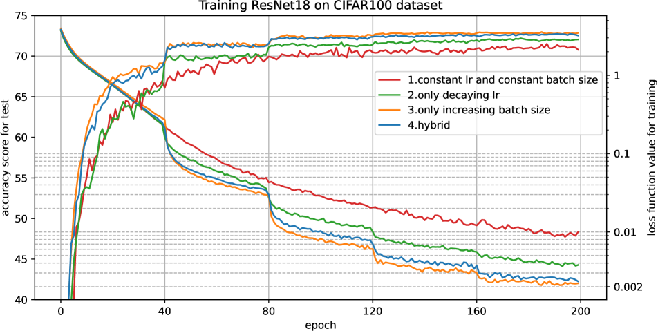
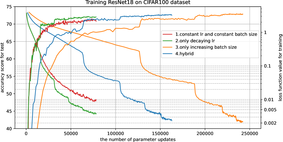
Figure 9: Accuracy score for testing and loss function value for training versus the number of epochs (left) and the number of parameter updates (right) in training ResNet18 on the CIFAR100 dataset. In method 1, the learning rate and the batch size were fixed at 0.1 and 128, respectively. In method 2, the learning rate decreased every 40 epochs as in $\left[0.1,\frac{1}{10\sqrt{2}},0.05,\frac{1}{20\sqrt{2}},0.025\right]$ and the batch size was fixed at 128. In method 3, the learning rate was fixed at 0.1, and the batch size was increased as $\left[16,32,64,128,256\right]$. In method 4, the learning rate was decreased as $\left[0.1,\frac{\sqrt{3}}{20},0.075,\frac{3\sqrt{3}}{80},0.05625\right]$ and the batch size was increased as $\left[32,48,72,108,162\right]$.

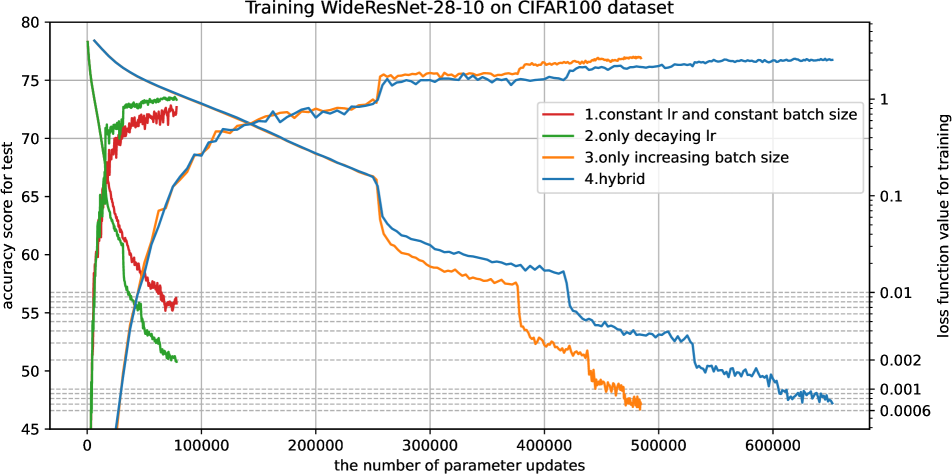
Figure 10: Accuracy score for testing and loss function value for training versus the number of epochs (left) and the number of parameter updates (right) in training WideResNet-28-10 on the CIFAR100 dataset. The left graph is the same graph as Figure 2. In method 1, the learning rate and batch size were fixed at 0.1 and 128, respectively. In method 2, the learning rate was decreased every 40 epochs as $\left[0.1,\frac{1}{10\sqrt{2}},0.05,\frac{1}{20\sqrt{2}},0.025\right]$ and the batch size was fixed at 128. In method 3, the learning rate was fixed at 0.1, and the batch size increased as $\left[8,16,32,64,128\right]$. In method 4, the learning rate decreased as $\left[0.1,\frac{\sqrt{3}}{20},0.075,\frac{3\sqrt{3}}{80},0.05625\right]$ and the batch size increased as $\left[8,12,18,27,40\right]$.

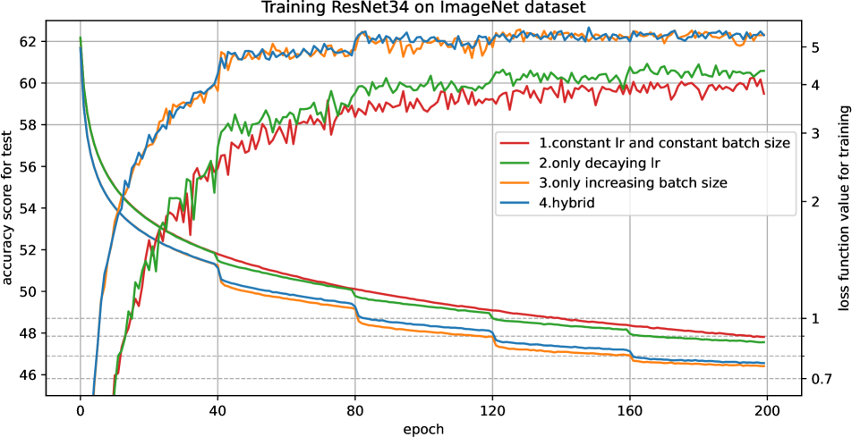
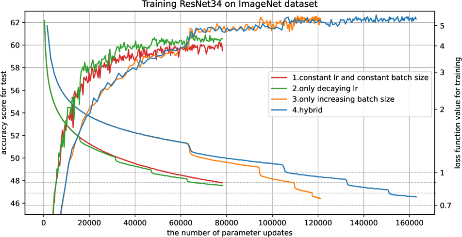
Figure 11: Accuracy score for testing and loss function value for training versus number of epochs (left) and the number of parameter updates (right) in training ResNet34 on the ImageNet dataset. In method 1, the learning rate and batch size were fixed at 0.1 and 256, respectively. In method 2, the learning rate was decreased every 40 epochs as $\left[0.1,\frac{1}{10\sqrt{2}},0.05,\frac{1}{20\sqrt{2}},0.025\right]$ and the batch size was fixed at 256. In method 3, the learning rate was fixed at 0.1, and the batch size was increased as $\left[32,64,128,256,512\right]$. In method 4, the learning rate was decreased as $\left[0.1,\frac{\sqrt{3}}{20},0.075,\frac{3\sqrt{3}}{80},0.05625\right]$ and the batch size was increased as $\left[32,48,72,108,162\right]$.

For methods 2, 3, and 4, the decay rates are all $1/\sqrt{2}$, and the decay intervals are all 40 epochs, so throughout the training, the three methods should theoretically be optimizing the exact same five smoothed functions in sequence. Nevertheless, the local solutions reached by each of the three methods are not exactly the same. All results indicate that method 3 is superior to method 2 and that method 4 is superior to method 3 in both test accuracy and training loss function values. This difference can be attributed to the different learning rates used to optimize each smoothing function. Among methods 2, 3, and 4, method 3, which does not decay the learning rate, maintains the highest learning rate 0.1, followed by method 4 and method 2. In all graphs, the loss function values are always small in this order; i.e., the larger the learning rate is, the lower loss function values become. Therefore, we can say that the noise level $|\delta|$, expressed as $\frac{\eta C}{\sqrt{b}}$, needs to be reduced, while the learning rate $\eta$ needs to remain as large as possible. Alternatively, if the learning rate is small, then a large number of iterations are required. Thus, for the same rate of change and the same number of epochs, an increasing batch size is superior to a decreasing learning rate because an increasing batch size can maintain a large learning rate and can be made to iterate a lot when the batch size is small.

Theoretically, the noise level $|\delta_{m}|$ should gradually decrease and become zero at the end, so in our algorithm 3, the learning rate $\eta_{m}$ should be zero at the end or the batch size $b_{m}$ should match the number of data sets at the end. However, if the learning rate is 0, training cannot proceed, and if the batch size is close to a full batch, it is not feasible from a computational point of view. For this reason, the experiments described in this paper are not fully graduated optimizations; i.e., full global optimization is not achieved. In fact, the last batch size used by method 2 is around 128 to 512, which is far from a full batch. Therefore, the solution reached in this experiment is the optimal solution for a function that has been smoothed to some extent, and to achieve a global optimization of the DNN, it is necessary to increase only the batch size to eventually reach a full batch, or increase the number of iterations accordingly while increasing the batch size and decaying the learning rate.

Finally, we should note that graduated optimization with Algorithm 1 is not applicable to DNNs. Our approach, Algorithm 3, allows implicit graduated optimization by exploiting the smoothness of SGD; the experimental results provided in this section imply its success.

10.2 Experiments on Optimal Noise Scheduling

This section complements Section 4.2. We evaluated the performance of SGDs with several decaying learning rate schedules in training ResNet18 (Figure 12) and WideResNet-28-10 (Figure 13) on the CIFAR100 dataset. All experiments were run for 200 epochs and the batch size was fixed at 128. The learning rate was decreased per epoch; see Section 9 for the respective update rules.

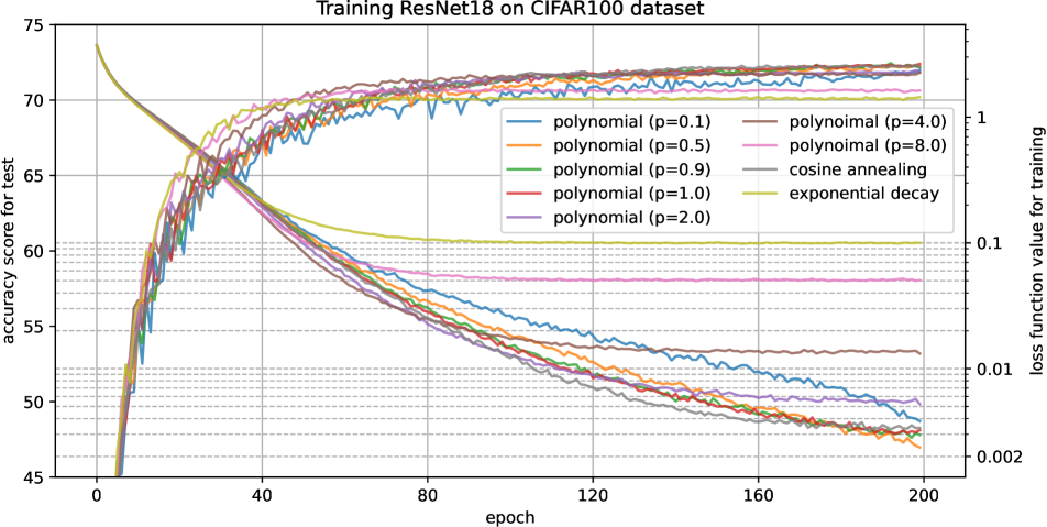
Figure 12: Accuracy score for testing and loss function value for training versus number of epochs in training ResNet18 on the CIFAR100 dataset. This is the same graph as in Figure 3. The average of multiple runs is plotted.

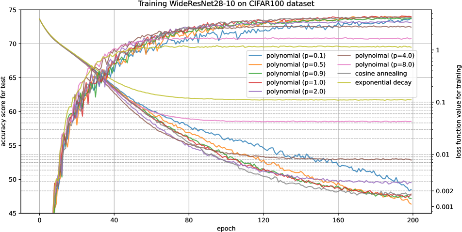
Figure 13: Accuracy score for testing and loss function value for training versus number of epochs in training WideResNet-28-10 on the CIFAR100 dataset. The average of multiple runs is plotted.

Both results show that a polynomial decay with a power less than or equal to 1, which is the schedule that satisfies the condition that $\gamma_{m}$ must satisfy, is superior in both test accuracy and training loss function value. Furthermore, the loss function values and test accuracy worsen the further away from the green region that the decay rate curve must satisfy (see Figure 6 and Figure 8), and the order is in excellent agreement with the order in which lower loss function values are achieved. According to Theorem 3.4, Algorithm 3 reaches an $\epsilon$-neighborhood of the globally optimal solution after $\mathcal{O}\left(1/\epsilon^{\frac{1}{p}}\right)$ iterations. Thus, theoretically, the closer $p$ is to 1, the fewer iterations are required. This explains why $p=0.1$ is not initially superior in both test accuracy and loss function value for training in Figures 12 and 13.

11 Lemmas used in the proofs of the theorems

Lemma 11.1.

Suppose that $F\colon\mathbb{R}^{d}\to\mathbb{R}$ is $\sigma$-strongly convex and $\hat{\bm{x}}_{t+1}:=\hat{\bm{x}}_{t}-\eta_{t}\bm{g}_{t}$. Then, for all $t\in\mathbb{N}$,

$$\mathbb{E}\left[F(\hat{\bm{x}}_{t})-F(\bm{x}^{\star})\right]\leq\frac{1-\sigma\eta_{t}}{2\eta_{t}}X_{t}-\frac{1}{2\eta_{t}}X_{t+1}+\frac{\eta_{t}}{2}\mathbb{E}\left[\|\bm{g}_{t}\|^{2}\right],$$ (71)

where $\bm{g}_{t}:=\nabla F_{\mathcal{S}_{t}}(\hat{\bm{x}}_{t})$, $X_{t}:=\mathbb{E}\left[\|\hat{\bm{x}}_{t}-\bm{x}^{\star}\|^{2}\right]$, and $\bm{x}^{\star}$ is the global minimizer of $F$.

Proof.

Let $t\in\mathbb{N}$. The definition of $\hat{\bm{x}}_{t+1}$ guarantees that

$$\|\hat{\bm{x}}_{t+1}-\bm{x}^{\star}\|^{2} =\|(\hat{\bm{x}}_{t}-\eta_{t}\bm{g}_{t})-\bm{x}^{\star}\|^{2}$$ (72)

$$=\|\hat{\bm{x}}_{t}-\bm{x}^{\star}\|^{2}-2\eta_{t}\langle\hat{\bm{x}}_{t}-\bm{x}^{\star},\bm{g}_{t}\rangle+\eta_{t}^{2}\|\bm{g}_{t}\|^{2}.$$ (73)

From the $\sigma$-strong convexity of $F$,

$$\mathbb{E}\left[\|\hat{\bm{x}}_{t+1}-\bm{x}^{\star}\|^{2}|\hat{\bm{x}}_{t}\right] =\|\hat{\bm{x}}_{t}-\bm{x}^{\star}\|^{2}-2\eta_{t}\langle\hat{\bm{x}}_{t}-\bm{x}^{\star},\nabla F(\hat{\bm{x}}_{t})\rangle+\eta_{t}^{2}\mathbb{E}\left[\|\bm{g}_{t}\|^{2}|\hat{\bm{x}}_{t}\right]$$ (74)

$$\leq\|\hat{\bm{x}}_{t}-\bm{x}^{\star}\|^{2}+2\eta_{t}\left(F(\bm{x}^{\star})-F(\hat{\bm{x}}_{t})-\frac{\sigma}{2}\|\hat{\bm{x}}_{t}-\bm{x}^{\star}\|^{2}\right)+\eta_{t}^{2}\mathbb{E}\left[\|\bm{g}_{t}\|^{2}|\hat{\bm{x}}_{t}\right].$$ (75)

By taking the total expectation on both sides, we find that

$$\mathbb{E}\left[\|\hat{\bm{x}}_{t+1}-\bm{x}^{\star}\|^{2}\right]\leq(1-\sigma\eta_{t})\mathbb{E}\left[\|\hat{\bm{x}}_{t}-\bm{x}^{\star}\|^{2}\right]+2\eta_{t}\mathbb{E}\left[F(\bm{x}^{\star})-F(\hat{\bm{x}}_{t})\right]+\eta_{t}^{2}\mathbb{E}\left[\|\bm{g}_{t}\|^{2}\right].$$ (76)

Hence,

$$\mathbb{E}\left[F(\hat{\bm{x}}_{t})-F(\bm{x}^{\star})\right]\leq\frac{1-\sigma\eta_{t}}{2\eta_{t}}\mathbb{E}\left[\|\hat{\bm{x}}_{t}-\bm{x}^{\star}\|^{2}\right]-\frac{1}{2\eta_{t}}\mathbb{E}\left[\|\hat{\bm{x}}_{t+1}-\bm{x}^{\star}\|^{2}\right]+\frac{\eta_{t}}{2}\mathbb{E}\left[\|\bm{g}_{t}\|^{2}\right].$$ (77)

This completes the proof. ∎

Lemma 11.2.

Suppose that (A3) holds, $F\colon\mathbb{R}^{d}\to\mathbb{R}$ is $L_{g}$-smooth, and $\hat{\bm{x}}_{t+1}:=\hat{\bm{x}}_{t}-\eta_{t}\bm{g}_{t}$. Then, for all $t\in\mathbb{N}$,

$$\eta_{t}\left(1-\frac{L_{g}\eta_{t}}{2}\right)\mathbb{E}\left[\|\nabla F(\hat{\bm{x}}_{t})\|^{2}\right]\leq\mathbb{E}\left[F(\hat{\bm{x}}_{t})\right]-\mathbb{E}\left[F(\hat{\bm{x}}_{t+1})\right]+\frac{L_{g}\eta_{t}^{2}C^{2}}{2}.$$ (78)

where $\bm{g}_{t}:=\nabla F_{\mathcal{S}_{t}}(\hat{\bm{x}}_{t})$ and $\bm{x}^{\star}$ is the global minimizer of $F$.

Proof.

From the $L_{g}$-smoothness of the $F$ and the definition of the $\hat{\bm{x}}_{t+1}$, we have, for all $t\in\mathbb{N}$,

$$F(\hat{\bm{x}}_{t+1}) \leq F(\hat{\bm{x}}_{t})+\langle\nabla F(\hat{\bm{x}}_{t}),\hat{\bm{x}}_{t+1}-\hat{\bm{x}}_{t}\rangle+\frac{L_{g}}{2}\|\hat{\bm{x}}_{t+1}-\hat{\bm{x}}_{t}\|^{2}$$ (79)

$$=F(\hat{\bm{x}}_{t})-\eta_{t}\langle\nabla F(\hat{\bm{x}}_{t}),\bm{g}_{t}\rangle+\frac{L_{g}\eta_{t}^{2}}{2}\|\bm{g}_{t}\|^{2}.$$ (80)

Assumption (A3) ensures that

$$\mathbb{E}\left[F(\hat{\bm{x}}_{t+1})|\hat{\bm{x}}_{t}\right] \leq F(\hat{\bm{x}}_{t})-\eta_{t}\langle\nabla F(\hat{\bm{x}}_{t}),\nabla F(\hat{\bm{x}}_{t})\rangle+\frac{L_{g}\eta_{t}^{2}}{2}\mathbb{E}\left[\|\bm{g}_{t}\|^{2}|\hat{\bm{x}}_{t}\right]$$ (81)

$$\leq F(\hat{\bm{x}}_{t})-\eta_{t}\|\nabla F(\hat{\bm{x}}_{t})\|^{2}+\frac{L_{g}\eta_{t}^{2}}{2}\left(C^{2}+\|\nabla F(\hat{\bm{x}}_{t})\|^{2}\right)$$ (82)

$$\leq F(\hat{\bm{x}}_{t})-\eta_{t}\left(1-\frac{L_{g}\eta_{t}}{2}\right)\|\nabla F(\hat{\bm{x}}_{t})\|^{2}+\frac{L_{g}\eta_{t}^{2}C^{2}}{2}.$$ (83)

By taking the total expectation on both sides, we find that

$$\mathbb{E}\left[F(\hat{\bm{x}}_{t+1})\right]\leq\mathbb{E}\left[F(\hat{\bm{x}}_{t})\right]-\eta_{t}\left(1-\frac{L_{g}\eta_{t}}{2}\right)\mathbb{E}\left[\|\nabla F(\hat{\bm{x}}_{t})\|^{2}\right]+\frac{L_{g}\eta_{t}^{2}C^{2}}{2}.$$ (84)

Therefore, we have

$$\eta_{t}\left(1-\frac{L_{g}\eta_{t}}{2}\right)\mathbb{E}\left[\|\nabla F(\hat{\bm{x}}_{t})\|^{2}\right]\leq\mathbb{E}\left[F(\hat{\bm{x}}_{t})\right]-\mathbb{E}\left[F(\hat{\bm{x}}_{t+1})\right]+\frac{L_{g}\eta_{t}^{2}C^{2}}{2}.$$ (85)

This completes the proof. ∎

Lemma 11.3.

Suppose that (A3) holds, $F\colon\mathbb{R}^{d}\to\mathbb{R}$ is $L_{g}$-smooth, $\hat{\bm{x}}_{t+1}:=\hat{\bm{x}}_{t}-\eta_{t}\bm{g}_{t}$, and $\eta_{t}:=\eta<\frac{2}{L_{g}}$. Then, for all $t\in\mathbb{N}$,

$$\frac{1}{T}\sum_{t=1}^{T}\mathbb{E}\left[\|\bm{g}_{t}\|^{2}\right]\leq\frac{2\mathbb{E}\left[F(\hat{\bm{x}}_{1})-F(\bm{x}^{\star})\right]}{\eta\left(2-L_{g}\eta\right)T}+\frac{2C^{2}}{2-L_{g}\eta},$$ (86)

where $\bm{g}_{t}:=\nabla f_{\mathcal{S}_{t}}(\hat{\bm{x}}_{t})$ and $\bm{x}^{\star}$ is the global minimizer of $F$.

Proof.

According to Lemma 11.2, we have

$$\eta\left(1-\frac{L_{g}\eta}{2}\right)\mathbb{E}\left[\|\nabla F(\bm{x}_{t})\|^{2}\right]\leq\mathbb{E}\left[F(\hat{\bm{x}}_{t})\right]-\mathbb{E}\left[F(\hat{\bm{x}}_{t+1})\right]+\frac{L_{g}\eta^{2}C^{2}}{2}.$$ (87)

Summing over $t$, we find that

$$\eta\left(1-\frac{L_{g}\eta}{2}\right)\frac{1}{T}\sum_{t=1}^{T}\mathbb{E}\left[\|\nabla F(\hat{\bm{x}}_{t})\|^{2}\right]\leq\frac{\mathbb{E}\left[F(\hat{\bm{x}}_{1})\right]-\mathbb{E}\left[F(\hat{\bm{x}}_{T+1})\right]}{T}+\frac{L_{g}\eta^{2}C^{2}}{2}.$$ (88)

From (A3), $\mathbb{E}\left[\|\bm{g}_{t}\|^{2}\right]\leq C^{2}+\mathbb{E}\left[\|\nabla F(\hat{\bm{x}}_{t})\|^{2}\right]$. Then, we have

$$\eta\left(1-\frac{L_{g}\eta}{2}\right)\left(\frac{1}{T}\sum_{t=1}^{T}\mathbb{E}\left[\|\bm{g}_{t}\|^{2}\right]-C^{2}\right)\leq\frac{\mathbb{E}\left[F(\hat{\bm{x}}_{1})\right]-\mathbb{E}\left[F(\hat{\bm{x}}_{T+1})\right]}{T}+\frac{L_{g}\eta^{2}C^{2}}{2}.$$ (89)

Hence, from $\eta<\frac{2}{L_{g}}$,

$$\frac{1}{T}\sum_{t=1}^{T}\mathbb{E}\left[\|\bm{g}_{t}\|^{2}\right] \leq\frac{2\mathbb{E}\left[F(\hat{\bm{x}}_{1})-F(\bm{x}^{\star})\right]}{\eta\left(2-L_{g}\eta\right)T}+\frac{L_{g}\eta C^{2}}{2-L_{g}\eta}+C^{2}$$ (90)

$$=\frac{2\mathbb{E}\left[F(\hat{\bm{x}}_{1})-F(\bm{x}^{\star})\right]}{\eta\left(2-L_{g}\eta\right)T}+\frac{2C^{2}}{2-L_{g}\eta}.$$ (91)

This completes the proof. ∎

Lemma 11.4.

Suppose that (A3) holds, $F\colon\mathbb{R}^{d}\to\mathbb{R}$ is $L_{g}$-smooth, $\hat{\bm{x}}_{t+1}:=\hat{\bm{x}}_{t}-\eta_{t}\bm{g}_{t}$, and $\eta_{t}:=\frac{2}{\sigma t}$. Then, for all $t\in\mathbb{N}$,

$$\mathbb{E}\left[\|\bm{g}_{t}\|^{2}\right]\leq B_{2},$$ (92)

where $B_{2}\geq 0$ is a nonnegative constant.

Proof.

According to Lemma 11.2, we have

$$\eta_{t}\left(1-\frac{L_{g}\eta_{t}}{2}\right)\mathbb{E}\left[\|\nabla F(\hat{\bm{x}}_{t})\|^{2}\right]\leq\mathbb{E}\left[F(\hat{\bm{x}}_{t})\right]-\mathbb{E}\left[F(\hat{\bm{x}}_{t+1})\right]+\frac{L_{g}\eta_{t}^{2}C^{2}}{2}.$$ (93)

Summing over $t$ from $t=t_{0}$ to $t=T$, we have

$$\sum_{t=t_{0}}^{T}\eta_{t}\left(1-\frac{L_{g}\eta_{t}}{2}\right)\mathbb{E}\left[\|\nabla F(\hat{\bm{x}}_{t})\|^{2}\right]\leq\mathbb{E}\left[F(\hat{\bm{x}}_{t_{0}})\right]-\mathbb{E}\left[F(\hat{\bm{x}}_{T})\right]+\frac{L_{g}C^{2}}{2}\sum_{t={t_{0}}}^{T}\eta_{t}^{2},$$ (94)

where $t_{0}$ satisfies

$$\forall t\geq t_{0}\colon\eta_{t_{0}}<\frac{2}{L_{g}}.$$ (95)

From $\sum_{t=0}^{\infty}\eta_{t}^{2}<\infty$, we obtain

$$\left(1-\frac{L_{g}\eta_{t_{0}}}{2}\right)\sum_{t=t_{0}}^{T}\eta_{t}\mathbb{E}\left[\|\nabla F(\hat{\bm{x}}_{t})\|^{2}\right]\leq\underbrace{\mathbb{E}\left[F(\hat{\bm{x}}_{t_{0}})\right]-\mathbb{E}\left[F(\bm{x}^{\star})\right]+\frac{L_{g}C^{2}}{2}\sum_{t={t_{0}}}^{\infty}\eta_{t}^{2}}_{=:B}<\infty.$$ (96)

Then,

$$\sum_{t=t_{0}}^{T}\eta_{t}\mathbb{E}\left[\|\nabla F(\hat{\bm{x}}_{t})\|^{2}\right]\leq\frac{2B}{2-L_{g}\eta_{t_{0}}}<\infty.$$ (97)

Therefore,

$$\sum_{t=1}^{T}\eta_{t}\mathbb{E}\left[\|\nabla F(\hat{\bm{x}}_{t})\|^{2}\right]\leq\frac{2B}{2-L_{g}\eta_{t_{0}}}+\sum_{t=1}^{{t_{0}}-1}\eta_{t}\mathbb{E}\left[\|\nabla F(\hat{\bm{x}}_{t})\|^{2}\right]<\infty.$$ (98)

From (98) and $\sum_{t=1}^{\infty}\eta_{t}=\infty$,

$$\liminf_{t\to\infty}\mathbb{E}\left[\|\nabla F(\hat{\bm{x}}_{t})\|^{2}\right]\leq 0$$ (99)

Hence, $\displaystyle\liminf_{t\to\infty}\mathbb{E}\left[\|\nabla F(\hat{\bm{x}}_{t})\|^{2}\right]=0$; i.e., $\mathbb{E}\left[\|\nabla F(\hat{\bm{x}}_{t})\|^{2}\right]$ is bounded. Let its upper boundary be $B_{1}$. Then Assumption (A3) ensures that

$$\mathbb{E}\left[\|\bm{g}_{t}\|^{2}\right] \leq C^{2}+\mathbb{E}\left[\|\nabla F(\hat{\bm{x}}_{t})\|^{2}\right]$$ (100)

$$\leq C^{2}+B_{1}=:B_{2}$$ (101)

This completes the proof. ∎

12 Proof of the Theorems and Propositions

12.1 Proof of Theorem 3.1

Proof.

Lemma 11.1, Lemma 11.4, and $\eta_{t}:=\frac{2}{\sigma t}$ guarantee that

$$\mathbb{E}\left[F(\hat{\bm{x}}_{t})-F(\bm{x}^{\star})\right] \leq\frac{1-\sigma\eta_{t}}{2\eta_{t}}X_{t}-\frac{1}{2\eta_{t}}X_{t+1}+\frac{\eta_{t}}{2}\mathbb{E}\left[\|\bm{g}_{t}\|^{2}\right]$$ (102)

$$\leq\frac{1}{2\eta_{t}}\left\{(1-\sigma\eta_{t})X_{t}-X_{t+1}\right\}+\frac{\eta_{t}B_{2}}{2}$$ (103)

$$=\frac{\sigma(t-2)}{4}X_{t}-\frac{\sigma t}{4}X_{t+1}+\frac{B_{2}}{\sigma t}.$$ (104)

Therefore, we have

$$(t-1)\mathbb{E}\left[F(\hat{\bm{x}}_{t})-F(\bm{x}^{\star})\right]\leq\frac{\sigma(t-2)(t-1)}{4}X_{t}-\frac{\sigma(t-1)t}{4}X_{t+1}+\frac{B_{2}(t-1)}{\sigma t}.$$ (105)

Summing over $t$, we find that

$$\sum_{t=1}^{T}(t-1)\mathbb{E}\left[F(\hat{\bm{x}}_{t})-F(\bm{x}^{\star})\right] \leq\frac{\sigma\cdot(-1)\cdot 0}{4}X_{1}-\frac{\sigma(T-1)T}{4}X_{T+1}+\frac{B_{2}}{\sigma}\sum_{t=1}^{T}\frac{t-1}{t}$$ (106)

$$\leq\frac{B_{2}(T-1)}{\sigma}.$$ (107)

Then, we have

$$\frac{2}{(T-1)T}\sum_{t=1}^{T}(t-1)\mathbb{E}\left[F(\hat{\bm{x}}_{t})-F(\bm{x}^{\star})\right] \leq\frac{2B_{2}}{\sigma T}.$$ (108)

From the convexity of $F$,

$$F\left(\frac{2}{T(T-1)}\sum_{t=1}^{T}(t-1)\hat{\bm{x}}_{t}\right)\leq\frac{2}{T(T-1)}\sum_{t=1}^{T}(t-1)F(\hat{\bm{x}}_{t}).$$ (109)

Hence,

$$\mathbb{E}\left[F\left(\frac{2}{T(T-1)}\sum_{t=1}^{T}(t-1)\hat{\bm{x}}_{t}\right)-F(\bm{x}^{\star})\right]\leq\frac{2B_{2}}{\sigma T}=\mathcal{O}\left(\frac{1}{T}\right)$$ (110)

In addition, since the minimum value is smaller than the mean, we have

$$\min_{t\in[T]}\mathbb{E}\left[F\left(\hat{\bm{x}}_{t}\right)-F(\bm{x}^{\star})\right]\leq H_{4}\frac{1}{T}+H_{3}\eta=\mathcal{O}\left(\frac{1}{T}+\eta\right).$$ (111)

This completes the proof. ∎

12.2 Proof of Theorem 3.2

Proof.

From $M^{p}:=\frac{1}{\alpha_{0}\epsilon}$, $\delta_{1}:=\frac{2L_{f}}{\sigma r}$, and $\gamma_{m+1}:=\frac{(M-m)^{p}}{\left\{M-(m-1)\right\}^{p}}$, we have

$$\delta_{M} =\delta_{1}\left(\gamma_{1}\gamma_{2}\cdots\gamma_{M-1}\right)$$ (112)

$$=\delta_{1}\cdot\frac{(M-1)^{p}}{M^{p}}\cdot\frac{(M-2)^{p}}{(M-1)^{p}}\cdot\frac{(M-3)^{p}}{(M-2)^{p}}\cdots\frac{1}{2^{p}}$$ (113)

$$=\delta_{1}\cdot\frac{1}{M^{p}}$$ (114)

$$=\delta_{1}\alpha_{0}\epsilon$$ (115)

$$=\frac{2L_{f}\alpha_{0}\epsilon}{\sigma r}.$$ (116)

According to Theorem 3.1,

$$\mathbb{E}\left[\hat{f}_{\delta_{M}}(\bm{x}_{M+1})-\hat{f}_{\delta_{M}}(\bm{x}_{\delta_{M}}^{\star})\right] \leq\epsilon_{M}$$ (117)

$$=\sigma\delta_{M}^{2}$$ (118)

$$=\left(\frac{2L_{f}\alpha_{0}\epsilon}{\sqrt{\sigma}r}\right)^{2}$$ (119)

From Lemma 8.2 and 8.3,

$$f(\bm{x}_{M+2})-f(\bm{x}^{\star}) =\left\{f(\bm{x}_{M+2})-\hat{f}_{\delta_{M}}(\bm{x}_{M+2})\right\}+\left\{\hat{f}_{\delta_{M}}(\bm{x}^{\star})-f(\bm{x}^{\star})\right\}+\left\{\hat{f}_{\delta_{M}}(\bm{x}_{M+2})-\hat{f}_{\delta_{M}}(\bm{x}^{\star})\right\}$$ (120)

$$\leq\left\{f(\bm{x}_{M+2})-\hat{f}_{\delta_{M}}(\bm{x}_{M+2})\right\}+\left\{\hat{f}_{\delta_{M}}(\bm{x}^{\star})-f(\bm{x}^{\star})\right\}+\left\{\hat{f}_{\delta_{M}}(\bm{x}_{M+2})-\hat{f}_{\delta_{M}}(\bm{x}_{\delta_{M}}^{\star})\right\}$$ (121)

$$\leq\delta_{M}L_{f}+\delta_{M}L_{f}+\left\{\hat{f}_{\delta_{M}}(\bm{x}_{M+2})-\hat{f}_{\delta_{M}}(\bm{x}_{\delta_{M}}^{\star})\right\}$$ (122)

$$=2\delta_{M}L_{f}+\left\{\hat{f}_{\delta_{M}}(\bm{x}_{M+2})-\hat{f}_{\delta_{M}}(\bm{x}_{M+1})\right\}+\left\{\hat{f}_{\delta_{M}}(\bm{x}_{M+1})-\hat{f}_{\delta_{M}}(\bm{x}_{\delta_{M}}^{\star})\right\}$$ (123)

$$\leq 2\delta_{M}L_{f}+L_{f}\left\|\bm{x}_{M+2}-\bm{x}_{M+1}\right\|+\left\{\hat{f}_{\delta_{M}}(\bm{x}_{M+1})-\hat{f}_{\delta_{M}}(\bm{x}_{\delta_{M}}^{\star})\right\}.$$ (124)

Then, we have

$$\mathbb{E}\left[f(\bm{x}_{M+2})-f(\bm{x}^{\star})\right] \leq 2\delta_{M}L_{f}+2L_{f}d_{M}\delta_{M}+\epsilon_{M}$$ (125)

$$\leq 2\delta_{M}L_{f}+2L_{f}\bar{d}\delta_{M}+\epsilon_{M}$$ (126)

$$=2L_{f}\delta_{M}\left(1+\bar{d}\right)+\epsilon_{M},$$ (127)

where we have used $\left\|\bm{x}_{M+2}-\bm{x}_{M+1}\right\|\leq 2d_{M}\delta_{M}$ since $\bm{x}_{M+2},\bm{x}_{M+1}\in N(\bm{x}^{\star};d_{M}\delta_{M})$, and $d_{M}\leq\bar{d}<+\infty$. Therefore,

$$\mathbb{E}\left[f(\bm{x}_{M+2})-f(\bm{x}^{\star})\right] \leq 2L_{f}\left(1+\bar{d}\right)\frac{2L_{f}\alpha_{0}\epsilon}{\sigma r}+\left(\frac{2L_{f}\alpha_{0}\epsilon}{\sqrt{\sigma}r}\right)^{2}$$ (128)

$$=\frac{4L_{f}^{2}\left(1+\bar{d}\right)\alpha_{0}\epsilon}{\sigma r}+\left(\frac{2L_{f}\alpha_{0}\epsilon}{\sqrt{\sigma}r}\right)^{2}$$ (129)

$$\leq\epsilon,$$ (130)

where we have used $\alpha_{0}:=\min\left\{\frac{\sigma r}{8L_{f}^{2}\left(1+\bar{d}\right)},\frac{\sqrt{\sigma}r}{2\sqrt{2}L_{f}}\right\}$.
Let $T_{\text{total}}$ be the total number of queries made by Algorithm 1; then,

$$T_{\text{total}} =\sum_{m=1}^{M+1}\frac{2B_{2}}{\sigma\epsilon_{m}}=\sum_{m=1}^{M+1}\frac{2B_{2}}{\sigma^{2}\delta_{m}^{2}}$$ (131)

$$=\frac{2B_{2}}{\sigma^{2}\delta_{1}^{2}}\left(1+\frac{1}{\gamma_{1}^{2}}+\frac{1}{\gamma_{1}^{2}\gamma_{2}^{2}}+\cdots+\frac{2}{\gamma_{1}^{2}\gamma_{2}^{2}\cdots\gamma_{M-1}^{2}}\right)$$ (132)

$$=\frac{2B_{2}}{\sigma^{2}\delta_{1}^{2}}\left\{\frac{\left(\gamma_{1}^{2}\gamma_{2}^{2}\cdots\gamma_{M-1}^{2}\right)+\left(\gamma_{2}^{2}\gamma_{3}^{2}\cdots\gamma_{M-1}^{2}\right)+\cdots+\gamma_{M-1}^{2}+2}{\gamma_{1}^{2}\gamma_{2}^{2}\cdots\gamma_{M-1}^{2}}\right\}$$ (133)

From $\gamma_{1}\gamma_{2}\cdots\gamma_{M-1}=\frac{1}{M^{p}}$,

$$T_{\text{total}} =\frac{2B_{2}}{\sigma^{2}\delta_{1}^{2}}\cdot\frac{\frac{1}{M^{2p}}+\frac{1}{(M-1)^{2p}}+\frac{1}{(M-2)^{2p}}+\cdots\frac{1}{2^{2p}}+2}{\frac{1}{M^{2p}}}$$ (134)

$$\leq\frac{2B_{2}}{\sigma^{2}\delta_{1}^{2}}\cdot M^{2p}(M+1)$$ (135)

$$=\frac{2B_{2}}{\sigma^{2}\delta_{1}^{2}}\cdot M^{2p+1}+\frac{2B_{2}}{\sigma^{2}\delta_{1}^{2}}\cdot M^{2p}$$ (136)

$$=\frac{2B_{2}}{\sigma^{2}\delta_{1}^{2}}\left(\frac{1}{\alpha_{0}\epsilon}\right)^{\frac{1}{p}+2}+\frac{2B_{2}}{\sigma^{2}\delta_{1}^{2}}\left(\frac{1}{\alpha_{0}\epsilon}\right)^{2}$$ (137)

$$=\mathcal{O}\left(\frac{1}{\epsilon^{\frac{1}{p}+2}}\right),$$ (138)

This completes the proof. ∎

12.3 Proof of Theorem 3.3

Proof.

Lemma 11.1 guarantees that

$$\mathbb{E}\left[F(\hat{\bm{x}}_{t})-F(\bm{x}^{\star})\right] \leq\frac{1-\sigma\eta_{t}}{2\eta_{t}}X_{t}-\frac{1}{2\eta_{t}}X_{t+1}+\frac{\eta_{t}}{2}\mathbb{E}\left[\|\bm{g}_{t}\|^{2}\right]$$ (139)

$$=\frac{1-\sigma\eta}{2\eta}\left(X_{t}-X_{t+1}\right)-\frac{\sigma}{2}X_{t+1}+\frac{\eta}{2}\mathbb{E}\left[\|\bm{g}_{t}\|^{2}\right].$$ (140)

From $\eta<\min\left\{\frac{1}{\sigma},\frac{2}{L_{g}}\right\}$ and Lemma 11.3, by summing over $t$ we find that

$$\frac{1}{T}\sum_{t=1}^{T}\mathbb{E}\left[F(\hat{\bm{x}}_{t})-F(\bm{x}^{\star})\right] \leq\frac{1-\sigma\eta}{2\eta T}\left(X_{1}-X_{T+1}\right)-\frac{\sigma}{2T}\sum_{t=1}^{T}X_{t+1}+\frac{\eta}{2T}\sum_{t=1}^{T}\mathbb{E}\left[\|\bm{g}_{t}\|^{2}\right]$$ (141)

$$\leq\frac{1-\sigma\eta}{2\eta T}X_{1}+\frac{\eta}{2T}\sum_{t=1}^{T}\mathbb{E}\left[\|\bm{g}_{t}\|^{2}\right]$$ (142)

$$\leq\underbrace{\frac{\left(1-\sigma\eta\right)X_{1}}{2\eta}}_{=:H_{1}}\frac{1}{T}+\underbrace{\frac{\mathbb{E}\left[F(\hat{\bm{x}}_{1})-F(\bm{x}^{\star})\right]}{\left(2-L_{g}\eta\right)}}_{=:H_{2}}\frac{1}{T}+\underbrace{\frac{C^{2}}{\left(2-L_{g}\eta\right)}}_{=:H_{3}}\eta$$ (143)

$$=\underbrace{\left(H_{1}+H_{2}\right)}_{=:H_{4}}\frac{1}{T}+H_{3}\eta$$ (144)

$$=H_{4}\frac{1}{T}+H_{3}\eta,$$ (145)

where $H_{3}\text{ and }H_{4}>0$ are nonnegative constants. From the convexity of $F$,

$$F\left(\frac{1}{T}\sum_{t=1}^{T}\hat{\bm{x}}_{t}\right)\leq\frac{1}{T}\sum_{t=1}^{T}F(\hat{\bm{x}}_{t}).$$ (146)

Hence,

$$\mathbb{E}\left[F\left(\frac{1}{T}\sum_{t=1}^{T}\hat{\bm{x}}_{t}\right)-F(\bm{x}^{\star})\right]\leq H_{4}\frac{1}{T}+H_{3}\eta=\mathcal{O}\left(\frac{1}{T}+\eta\right).$$ (147)

In addition, since the minimum value is smaller than the mean, we have

$$\min_{t\in[T]}\mathbb{E}\left[F\left(\hat{\bm{x}}_{t}\right)-F(\bm{x}^{\star})\right]\leq H_{4}\frac{1}{T}+H_{3}\eta=\mathcal{O}\left(\frac{1}{T}+\eta\right).$$ (148)

This completes the proof. ∎

12.4 Proof of Theorem 3.4

Proof.

According to $\delta_{m+1}:=\frac{\eta_{m+1}C}{\sqrt{b_{m+1}}}$ and $\frac{\kappa_{m}}{\sqrt{\lambda_{m}}}=\gamma_{m}$, we have

$$\delta_{m+1} :=\frac{\eta_{m+1}C}{\sqrt{b_{m+1}}}$$ (149)

$$=\frac{\kappa_{m}\eta_{m}C}{\sqrt{\lambda_{m}}\sqrt{b_{m}}}$$ (150)

$$=\frac{\kappa_{m}}{\sqrt{\lambda_{m}}}\delta_{m}$$ (151)

$$=\gamma_{m}\delta_{m}.$$ (152)

Therefore, from $M^{p}:=\frac{1}{\alpha_{0}\epsilon}$, $\delta_{1}:=\frac{\eta_{1}C}{\sqrt{b_{1}}}$, and $\gamma_{m}:=\frac{(M-m)^{p}}{\left\{M-(m-1)\right\}^{p}}$, then

$$\delta_{M} =\delta_{1}\left(\gamma_{1}\gamma_{2}\cdots\gamma_{M-1}\right)$$ (153)

$$=\delta_{1}\cdot\frac{(M-1)^{p}}{M^{p}}\cdot\frac{(M-2)^{p}}{(M-1)^{p}}\cdot\frac{(M-3)^{p}}{(M-2)^{p}}\cdots\frac{1}{2^{p}}$$ (154)

$$=\delta_{1}\cdot\frac{1}{M^{p}}$$ (155)

$$=\delta_{1}\alpha_{0}\epsilon$$ (156)

$$=\frac{\eta_{1}C\alpha_{0}\epsilon}{\sqrt{b_{1}}}.$$ (157)

According to Theorem 3.3,

$$\mathbb{E}\left[\hat{f}_{\delta_{M}}(\bm{x}_{M+1})-\hat{f}_{\delta_{M}}(\bm{x}_{\delta_{M}}^{\star})\right] \leq\epsilon_{M}$$ (158)

$$=\sigma\delta_{M}^{2}$$ (159)

$$=\left(\frac{\sqrt{\sigma}\eta_{1}C\alpha_{0}\epsilon}{\sqrt{b_{1}}}\right)^{2}$$ (160)

As in the proof of Theorem 3.2, we have

$$\mathbb{E}\left[f(\bm{x}_{M+2})-f(\bm{x}^{\star})\right]\leq 2L_{f}\delta_{M}\left(1+\bar{d}\right)+\epsilon_{M}.$$ (161)

Therefore,

$$\mathbb{E}\left[f(\bm{x}_{M+2})-f(\bm{x}^{\star})\right] \leq 2L_{f}\left(1+\bar{d}\right)\frac{\eta_{1}C\alpha_{0}\epsilon}{\sqrt{b_{1}}}+\left(\frac{\sqrt{\sigma}\eta_{1}C\alpha_{0}\epsilon}{\sqrt{b_{1}}}\right)^{2}$$ (162)

$$=\frac{2L_{f}\left(1+\bar{d}\right)\eta_{1}C\alpha_{0}\epsilon}{\sqrt{b_{1}}}+\left(\frac{\sqrt{\sigma}\eta_{1}C\alpha_{0}\epsilon}{\sqrt{b_{1}}}\right)^{2}$$ (163)

$$\leq\epsilon,$$ (164)

where we have used $\alpha_{0}:=\min\left\{\frac{\sqrt{b_{1}}}{4L_{f}\eta_{1}C\left(1+\bar{d}\right)},\frac{\sqrt{b_{1}}}{\sqrt{2\sigma}\eta_{1}C}\right\}$.
Let $T_{\text{total}}$ be the total number of queries made by Algorithm 3; then,

$$T_{\text{total}} =\sum_{m=1}^{M+1}\frac{H_{4}}{\epsilon_{m}-H_{3}\eta_{m}}=\sum_{m=1}^{M+1}\frac{H_{4}}{\sigma^{2}\delta_{m}^{2}-H_{3}\eta_{m}}$$ (165)

$$=\frac{H_{4}}{\sigma^{2}\delta_{1}^{2}-H_{3}\eta_{1}}+\frac{H_{4}}{\sigma^{2}\delta_{2}^{2}-H_{3}\eta_{2}}+\cdots+\frac{2H_{4}}{\sigma^{2}\delta_{M}^{2}-H_{3}\eta_{M}}$$ (166)

$$\leq\frac{H_{4}(M+1)}{\sigma^{2}\delta_{M}^{2}-H_{3}\eta_{M}}$$ (167)

$$\leq\frac{H_{4}(M+1)}{\sigma^{2}\delta_{M}^{2}-H_{3}\eta_{1}}$$ (168)

$$=\frac{H_{4}(M+1)}{\sigma^{2}\delta_{1}^{2}\frac{1}{M^{2p}}-H_{3}\eta_{1}}$$ (169)

$$=\frac{H_{4}M^{2p}(M+1)}{\sigma^{2}\delta_{1}^{2}-H_{3}\eta_{1}M^{2p}}$$ (170)

$$=\frac{H_{4}M^{2p+1}}{\sigma^{2}\delta_{1}^{2}-H_{3}\eta_{1}M^{2p}}+\frac{H_{4}M^{2p}}{\sigma^{2}\delta_{1}^{2}-H_{3}\eta_{1}M^{2p}}$$ (171)

From $M^{p}:=\frac{1}{\alpha_{0}\epsilon}$,

$$T_{\text{total}} =\frac{H_{4}\left(\frac{1}{\alpha_{0}\epsilon}\right)^{\frac{1}{p}+2}}{\sigma^{2}\delta_{1}^{2}-H_{3}\eta_{1}\left(\frac{1}{\alpha_{0}\epsilon}\right)^{2}}+\frac{H_{4}\left(\frac{1}{\alpha_{0}\epsilon}\right)^{2}}{\sigma^{2}\delta_{1}^{2}-H_{3}\eta_{1}\left(\frac{1}{\alpha_{0}\epsilon}\right)^{2}}$$ (172)

$$\leq\frac{2H_{4}\left(\frac{1}{\alpha_{0}\epsilon}\right)^{\frac{1}{p}+2}}{\sigma^{2}\delta_{1}^{2}-H_{3}\eta_{1}\left(\frac{1}{\alpha_{0}\epsilon}\right)^{2}}$$ (173)

$$=\frac{2H_{4}\left(\frac{1}{\alpha_{0}\epsilon}\right)^{\frac{1}{p}}}{\sigma^{2}\delta_{1}^{2}(\alpha_{0}\epsilon)^{2}-H_{3}\eta_{1}}$$ (174)

$$=\frac{2H_{4}}{\sigma^{2}\delta_{1}^{2}(\alpha_{0}\epsilon)^{\frac{1}{p}+2}-H_{3}\eta_{1}(\alpha_{0}\epsilon)^{\frac{1}{p}}}$$ (175)

$$\leq\frac{2H_{4}}{\sigma^{2}\delta_{1}^{2}(\alpha_{0}\epsilon)^{\frac{1}{p}}-H_{3}\eta_{1}(\alpha_{0}\epsilon)^{\frac{1}{p}}}$$ (176)

$$=\mathcal{O}\left(\frac{1}{\epsilon^{\frac{1}{p}}}\right).$$ (177)

This completes the proof. ∎

12.5 Proof of Proposition 3.1

Proof.

For all $\bm{x}\in N(\bm{x}^{\star};a_{m}r)\ (a_{m}\geq 0)$, and all $\bm{u}_{m}\sim B(\bm{0};1)$, the quadratic equation

$$\delta_{m}^{2}-2\left\langle\bm{x}^{\star}-\bm{x},\bm{u}_{m}\right\rangle\delta_{m}+(a_{m}^{2}-1)r^{2}=0$$ (178)

for $\delta_{m}\in\mathbb{R}$ has solutions with probability $p(a_{m})$ when $a_{m}>1$ and always has solutions when $0\leq a_{m}\leq 1$.

Let us derive $p(a_{m})$. When $a_{m}>1$, the condition for the discriminant equation of (178) to be positive is as follows:

$$-1\leq\cos\theta\leq-\frac{r\sqrt{a^{2}-1}}{\|\bm{x}^{\star}-\bm{x}\|\|\bm{u}_{m}\|},\text{ or }\ \frac{r\sqrt{a^{2}-1}}{\|\bm{x}^{\star}-\bm{x}\|\|\bm{u}_{m}\|}\leq\cos\theta\leq 1,$$ (179)

where $\theta$ is the angle between $\bm{u}_{m}\sim B(\bm{0};1)$ and $\bm{x}^{\star}-\bm{x}$. Note that $\cos\theta$ can be positive or negative because $\delta_{m}\in\mathbb{R}$. Since the random variable $\bm{u}_{m}$ is sampled uniformly from the $B(\bm{0};1)$, the probability that $\bm{u}_{m}$ satisfies (179) is less than

$$p(a_{m}):=\frac{2\arccos\left(\frac{r\sqrt{a_{m}^{2}-1}}{\|\bm{x}^{\star}-\bm{x}\|\|\bm{u}_{m}\|}\right)}{\pi},$$ (180)

for $\delta_{m}>0$ and $\delta_{m}<0$, respectively.

Now let us consider the solution of the quadratic inequality,

$$\|\bm{u}_{m}\|^{2}\delta_{m}^{2}-2\left\langle\bm{x}^{\star}-\bm{x},\bm{u}_{m}\right\rangle\delta_{m}+(a_{m}^{2}-1)r^{2}\leq 0$$ (181)

for $\delta_{m}\in\mathbb{R}$.

(i) When $a_{m}>1$, (181) has one or two solutions with probability $p(a_{m})$ or less. When $\frac{r\sqrt{a^{2}-1}}{\|\bm{x}^{\star}-\bm{x}\|\|\bm{u}_{m}\|}\leq\cos\theta\leq 1$, let the larger solution be $\delta^{+}>0$ and the smaller one be $\delta^{-}>0$; we can express these solutions as follows:

$$\delta^{+}:=\|\bm{x}^{\star}-\bm{x}\|\|\bm{u}_{m}\|\cos\theta+\sqrt{\|\bm{x}^{\star}-\bm{x}\|^{2}\|\bm{u}_{m}\|^{2}\cos^{2}\theta-r^{2}(a^{2}-1)},$$ (182)

$$\delta^{-}:=\|\bm{x}^{\star}-\bm{x}\|\|\bm{u}_{m}\|\cos\theta-\sqrt{\|\bm{x}^{\star}-\bm{x}\|^{2}\|\bm{u}_{m}\|^{2}\cos^{2}\theta-r^{2}(a^{2}-1)}.$$ (183)

Thus, the solution to (181) is

$$0<\delta^{-}<\delta_{m}<\delta^{+}$$ (184)

when $\frac{r\sqrt{a^{2}-1}}{\|\bm{x}^{\star}-\bm{x}\|\|\bm{u}_{m}\|}\leq\cos\theta\leq 1$, and

$$-\delta^{+}<\delta_{m}<-\delta^{-}<0$$ (185)

when $-1\leq\cos\theta\leq-\frac{r\sqrt{a^{2}-1}}{\|\bm{x}^{\star}-\bm{x}\|\|\bm{u}_{m}\|}$. Hence, we have

$$|\delta^{-}|\leq|\delta_{m}|\leq|\delta^{+}|.$$ (186)

(ii) When $a_{m}\leq 1$, (181) always has one or two solutions. The two solutions are defined as in (i). Then, the solution to (181) is

$$\delta^{-}<\delta_{m}<\delta^{+}\ (\delta^{-}<0,\delta^{+}>0)$$ (187)

when $\frac{r\sqrt{a^{2}-1}}{\|\bm{x}^{\star}-\bm{x}\|\|\bm{u}_{m}\|}\leq\cos\theta\leq 1$, and

$$-\delta^{+}<\delta_{m}<-\delta^{-}\ (-\delta^{+}<0,-\delta^{-}>0)$$ (188)

when $-1\leq\cos\theta\leq-\frac{r\sqrt{a^{2}-1}}{\|\bm{x}^{\star}-\bm{x}\|\|\bm{u}_{m}\|}$. Hence, we have

$$|\delta_{m}|\leq|\delta^{-}|.$$ (189)

From (i) and (ii), (181) may have a solution for all $a_{m}>0$ when $|\delta_{m}|=|\delta^{-}|$. Therefore, suppose $|\delta_{m}|=|\delta^{-}|$; then,

$$r^{2} \geq a_{m}^{2}r^{2}-2\delta_{m}\langle\bm{x}^{\star}-\bm{x},\bm{u}_{m}\rangle+|\delta_{m}|^{2}$$ (190)

$$\geq a_{m}^{2}r^{2}-2\delta_{m}\langle\bm{x}^{\star}-\bm{x},\bm{u}_{m}\rangle+|\delta_{m}|^{2}\|\bm{u}_{m}\|^{2}$$ (191)

$$>\|\bm{x}-\bm{x}^{\star}\|^{2}-2\delta_{m}\langle\bm{x}^{\star}-\bm{x},\bm{u}_{m}\rangle+|\delta_{m}|^{2}\|\bm{u}_{m}\|^{2}$$ (192)

$$=\|\bm{x}+\delta_{m}\bm{u}_{m}-\bm{x}^{\star}\|^{2}.$$ (193)

This means $\bm{x}+\delta_{m}\bm{u}_{m}\in N(\bm{x}^{\star};r)\ (\delta_{m}\in\mathbb{R})$, where $\bm{u}_{m}\sim B(\bm{0};1)$. Hence, for all $\bm{x},\bm{y}\in N(\bm{x}^{\star};a_{m}r)\subset\mathbb{R}^{d}\ (a_{m}>\sqrt{2})$,

$$\left\langle\nabla\hat{f}_{\delta_{m}}(\bm{x})-\nabla\hat{f}_{\delta_{m}}(\bm{y}),\bm{x}-\bm{y}\right\rangle =\left\langle\nabla\mathbb{E}_{\bm{u}}[f(\bm{x}+\delta_{m}\bm{u})]-\nabla\mathbb{E}_{\bm{u}}[f(\bm{y}+\delta_{m}\bm{u})],\bm{x}-\bm{y}\right\rangle$$ (194)

$$=\left\langle\mathbb{E}_{\bm{u}}[\nabla f(\bm{x}+\delta_{m}\bm{u})]-\mathbb{E}_{\bm{u}}[\nabla f(\bm{y}+\delta_{m}\bm{u})],\bm{x}-\bm{y}\right\rangle$$ (195)

$$=\left\langle\mathbb{E}_{\bm{u}}[\nabla f(\bm{x}+\delta_{m}\bm{u})-\nabla f(\bm{y}+\delta_{m}\bm{u})],\bm{x}-\bm{y}\right\rangle$$ (196)

$$=\mathbb{E}_{\bm{u}}[\left\langle\nabla f(\bm{x}+\delta_{m}\bm{u})-\nabla f(\bm{y}+\delta_{m}\bm{u}),\bm{x}-\bm{y}\right\rangle]$$ (197)

$$\geq\mathbb{E}_{\bm{u}}[\sigma\|(\bm{x}+\delta_{m}\bm{u})-(\bm{y}+\delta_{m}\bm{u})\|^{2}]$$ (198)

$$=\mathbb{E}_{\bm{u}}[\sigma\|\bm{x}-\bm{y}\|^{2}]$$ (199)

$$=\sigma\|\bm{x}-\bm{y}\|^{2}.$$ (200)

This means that if $|\delta_{m}|=|\delta^{-}|$ holds, then $\hat{f}_{\delta_{m}}$ is $\sigma$-strongly convex on $N(\bm{x}^{\star};a_{m}r)\ (a_{m}>\sqrt{2})$ when $f$ is $\sigma$-strongly convex on $B(\bm{x}^{\star};r)$. Also, if we define $d_{m}:=\frac{a_{m}r}{|\delta^{-}|}$, then $d_{m}|\delta_{m}|\leq a_{m}r$ holds; i.e., $\hat{f}_{\delta_{m}}$ is $\sigma$-strongly convex on $N(\bm{x}^{\star};d_{m}|\delta_{m}|)$. This completes the proof. ∎

12.6 Proof of Proposition 3.2

Proof.

From Proposition 3.1, for all $|\delta_{m}|=|\delta^{-}|$, $\hat{f}_{\delta_{m}}$ is $\sigma$-strongly convex, i.e.,

$$\sigma\|\bm{x}^{\star}-\bm{x}_{\delta_{m}}^{\star}\|^{2} \leq\left\langle\bm{x}^{\star}-\bm{x}_{\delta_{m}}^{\star},\nabla\hat{f}_{\delta_{m}}(\bm{x}^{\star})-\nabla\hat{f}_{\delta_{m}}(\bm{x}_{\delta_{m}}^{\star})\right\rangle$$ (201)

$$\leq\left\|\bm{x}^{\star}-\bm{x}_{\delta_{m}}^{\star}\right\|\left\|\nabla\hat{f}_{\delta_{m}}(\bm{x}^{\star})\right\|,$$ (202)

where we have used the Cauchy-Schwarz inequality and $\left\|\nabla\hat{f}_{\delta_{m}}(\bm{x}_{\delta_{m}}^{\star})\right\|=\bm{0}$. Accordingly, we have

$$\left\|\bm{x}^{\star}-\bm{x}_{\delta_{m}}^{\star}\right\|\left(\sigma\left\|\bm{x}^{\star}-\bm{x}_{\delta_{m}}^{\star}\right\|-\left\|\nabla\hat{f}_{\delta_{m}}(\bm{x}^{\star})\right\|\right)\leq 0.$$ (203)

Because $\left\|\bm{x}^{\star}-\bm{x}_{\delta_{m}}^{\star}\right\|\geq 0$,

$$\left\|\bm{x}^{\star}-\bm{x}_{\delta_{m}}^{\star}\right\|\leq\frac{\left\|\nabla\hat{f}_{\delta_{m}}(\bm{x}^{\star})\right\|}{\sigma}.$$ (204)

Hence,

$$\left\|\bm{x}_{\delta_{m}}^{\star}-\bm{x}_{\delta_{m+1}}^{\star}\right\| \leq\left\|\bm{x}_{\delta_{m}}^{\star}-\bm{x}^{\star}\right\|+\left\|\bm{x}_{\delta_{m+1}}-\bm{x}^{\star}\right\|$$ (205)

$$\leq\frac{1}{\sigma}\left(\left\|\nabla\hat{f}_{\delta_{m}}(\bm{x}^{\star})\right\|+\left\|\nabla\hat{f}_{\delta_{m+1}}(\bm{x}^{\star})\right\|\right)$$ (206)

$$\leq\frac{2}{\sigma}\max\left\{\left\|\nabla\hat{f}_{\delta_{m}}(\bm{x}^{\star})\right\|,\left\|\nabla\hat{f}_{\delta_{m+1}}(\bm{x}^{\star})\right\|\right\}$$ (207)

$$\leq|\delta_{m}|(1-\gamma_{m})$$ (208)

$$=|\delta_{m}|-|\delta_{m+1}|$$ (209)

This completes the proof. ∎

12.7 Proof of Proposition 3.3

Proof.

By using the triangle inequality, we have, for all $m\in[M]$,

$$\|\bm{x}_{m}^{\star}-\bm{x}^{\star}\| =\|\bm{x}_{m}^{\star}-\bm{x}_{m+1}^{\star}+\bm{x}_{m+1}^{\star}-\bm{x}^{\star}\|$$ (210)

$$\leq\|\bm{x}_{m}^{\star}-\bm{x}_{m+1}^{\star}\|+\|\bm{x}_{m+1}^{\star}-\bm{x}^{\star}\|$$ (211)

$$\leq\|\bm{x}_{m}^{\star}-\bm{x}_{m+1}^{\star}\|+\|\bm{x}_{m+1}^{\star}-\bm{x}_{m+2}^{\star}\|+\cdots+\|\bm{x}_{M}^{\star}-\bm{x}_{M+1}^{\star}\|+\|\bm{x}_{M+1}^{\star}-\bm{x}^{\star}\|$$ (212)

$$\leq(|\delta_{m}|-|\delta_{m+1}|)+(|\delta_{m+1}|-|\delta_{m+2}|)+\cdots+(|\delta_{M}|-|\delta_{M+1}|)+0$$ (213)

$$=|\delta_{m}|$$ (214)

$$=\frac{|\delta_{m+1}|}{\gamma_{m}}$$ (215)

$$<d_{m+1}|\delta_{m+1}|.$$ (216)

where we have used $\bm{x}_{M+1}^{\star}=\bm{x}^{\star}$, $\delta_{M+1}=0$, and $\gamma_{m}\in\left(\frac{1}{d_{m+1}},1\right)\ (\forall m\in[M-1])$. This completes the proof. ∎

References

- Allgower and Georg [1990] Eugene L. Allgower and Kurt Georg. Numerical continuation methods - an introduction. Springer, 1990.
- Antonante et al. [2022] Pasquale Antonante, Vasileios Tzoumas, Heng Yang, and Luca Carlone. Outlier-robust estimation: Hardness, minimally tuned algorithms, and applications. IEEE Transactions on Robotics, 38(1):281–301, 2022.
- Balles et al. [2017] Lukas Balles, Javier Romero, and Philipp Hennig. Coupling adaptive batch sizes with learning rates. In Proceedings of the 33rd Conference on Uncertainty in Artificial Intelligence, 2017.
- Black and Rangarajan [1996] Michael J. Black and Anand Rangarajan. On the unification of line processes, outlier rejection, and robust statistics with applications in early vision. International Journal of Computer Vision, 19(1):57–91, 1996.
- Blake and Zisserman [1987] Andrew Blake and Andrew Zisserman. Visual Reconstruction. MIT Press, 1987.
- Bottou et al. [2018] Léon Bottou, Frank E. Curtis, and Jorge Nocedal. Optimization methods for large-scale machine learning. SIAM Review, 60(2):223–311, 2018.
- Brox and Malik [2011] Thomas Brox and Jitendra Malik. Large displacement optical flow: Descriptor matching in variational motion estimation. IEEE Transactions on Pattern Analysis and Machine Learning, 33(3):500–513, 2011.
- Byrd et al. [2012] Richard H. Byrd, Gillian M. Chin, Jorge Nocedal, and Yuchen Wu. Sample size selection in optimization methods for machine learning. Mathematical Programming, 134(1):127–155, 2012.
- Chapelle and Wu [2010] Olivier Chapelle and Mingrui Wu. Gradient descent optimization of smoothed information retrieval metrics. Information retrieval, 13(3):216–235, 2010.
- Chapelle et al. [2006] Olivier Chapelle, Mingmin Chi, and Alexander Zien. A continuation method for semi-supervised SVMs. In Proceedings of the 23rd International Conference on Machine Learning, pages 185–192, 2006.
- Chapelle et al. [2008] Olivier Chapelle, Vikas Sindhwani, and S. Sathiya Keerthi. Optimization techniques for semi-supervised support vector machines. Journal of Machine Learning Research, 9:203–233, 2008.
- Chen et al. [2021] Jinghui Chen, Dongruo Zhou, Yiqi Tang, Ziyan Yang, Yuan Cao, and Quanquan Gu. Closing the generalization gap of adaptive gradient methods in training deep neural networks. In Proceedings of the Twenty-Ninth International Joint Conference on Artificial Intelligence, pages 3267–3275, 2021.
- Chen et al. [2017] Liang-Chieh Chen, George Papandreou, Florian Schroff, and Hartwig Adam. Rethinking atrous convolution for semantic image segmentation. http://arxiv.org/abs/1706.05587, 2017.
- Chen et al. [2018] Liang-Chieh Chen, George Papandreou, Iasonas Kokkinos, Kevin Murphy, and Alan L. Yuille. Deeplab: Semantic image segmentation with deep convolutional nets, atrous convolution, and fully connected crfs. IEEE Transactions on Pattern Analysis and Machine Learning, 40(4):834–848, 2018.
- Chen [2023] Ting Chen. On the importance of noise scheduling for diffusion models. https://arxiv.org/abs/2301.10972, 2023.
- Chen et al. [2023] Ting Chen, Lala Li, Saurabh Saxena, Geoffrey E. Hinton, and David J. Fleet. A generalist framework for panoptic segmentation of images and videos. In Proceedings of the IEEE/CVF International Conference on Computer Vision (ICCV), pages 909–919, 2023.
- Chen et al. [2019] Xiangyi Chen, Sijia Liu, Ruoyu Sun, and Mingyi Hong. On the convergence of a class of Adam-type algorithms for non-convex optimization. Proceedings of the 7th International Conference on Learning Representations, 2019.
- Daneshmand et al. [2018] Hadi Daneshmand, Jonas Moritz Kohler, Aurélien Lucchi, and Thomas Hofmann. Escaping saddles with stochastic gradients. In Proceedings of the 35th International Conference on Machine Learning, pages 1163–1172, 2018.
- De et al. [2017] Soham De, Abhay Kumar Yadav, David W. Jacobs, and Tom Goldstein. Automated inference with adaptive batches. In Proceedings of the 20th International Conference on Artificial Intelligence and Statistics, pages 1504–1513, 2017.
- Deng et al. [2009] Jia Deng, Wei Dong, Richard Socher, Li-Jia Li, Kai Li, and Li Fei-Fei. ImageNet: A large-scale hierarchical image database. In IEEE Computer Society Conference on Computer Vision and Pattern Recognition, pages 248–255, 2009.
- Fehrman et al. [2020] Benjamin Fehrman, Benjamin Gess, and Arnulf Jentzen. Convergence rates for the stochastic gradient descent method for non-convex objective functions. Journal of Machine Learning Research, 21:1–48, 2020.
- Friedlander and Schmidt [2012] Michael P. Friedlander and Mark Schmidt. Hybrid deterministic-stochastic methods for data fitting. SIAM Journal on Scientific Computing, 34(3), 2012.
- Ge et al. [2015] Rong Ge, Furong Huang, Chi Jin, and Yang Yuan. Escaping from saddle points - online stochastic gradient for tensor decomposition. In Proceedings of the 28th Conference on Learning Theory, pages 797–842, 2015.
- Gotmare et al. [2019] Akhilesh Gotmare, Nitish Shirish Keskar, Caiming Xiong, and Richard Socher. A closer look at deep learning heuristics: Learning rate restarts, warmup and distillation. In Proceedings of the 7th International Conference on Learning Representations, 2019.
- Goyal et al. [2017] Priya Goyal, Piotr Dollár, Ross B. Girshick, Pieter Noordhuis, Lukasz Wesolowski, Aapo Kyrola, Andrew Tulloch, Yangqing Jia, and Kaiming He. Accurate, large minibatch SGD: training imagenet in 1 hour. https://arxiv.org/abs/1706.02677, 2017.
- Hardt et al. [2016] Moritz Hardt, Ben Recht, and Yoram Singer. Train faster, generalize better: Stability of stochastic gradient descent. In Proceedings of The 33rd International Conference on Machine Learning, pages 1225–1234, 2016.
- Harshvardhan and Stich [2021] Harshvardhan and Sebastian U. Stich. Escaping local minima with stochastic noise. In the 13th International OPT Workshop on Optimization for Machine Learning in NeurIPS 2021, 2021.
- Hazan et al. [2016] Elad Hazan, Kfir Yehuda, and Shai Shalev-Shwartz. On graduated optimization for stochastic non-convex problems. In Proceedings of The 33rd International Conference on Machine Learning, pages 1833–1841, 2016.
- He et al. [2019] Fengxiang He, Tongliang Liu, and Dacheng Tao. Control batch size and learning rate to generalize well: Theoretical and empirical evidence. In Proceedings of the 32nd International Conference on Neural Information Processing Systems, pages 1141–1150, 2019.
- He et al. [2016] Kaiming He, Xiangyu Zhang, Shaoqing Ren, and Jian Sun. Deep residual learning for image recognition. In IEEE Conference on Computer Vision and Pattern Recognition, pages 770–778, 2016.
- Ho et al. [2020] Jonathan Ho, Ajay Jain, and Pieter Abbeel. Denoising diffusion probabilistic models. In Proceedings of the 34th Conference on Neural Information Processing Systems, 2020.
- Hoffer et al. [2017] Elad Hoffer, Itay Hubara, and Daniel Soudry. Train longer, generalize better: closing the generalization gap in large batch training of neural networks. In Proceedings of the 31st International Conference on Neural Information Processing Systems, pages 1731–1741, 2017.
- Hundt et al. [2019] Andrew Hundt, Varun Jain, and Gregory D. Hager. sharpDARTS: faster and more accurate differentiable architecture search. https://arxiv.org/abs/1903.09900, 2019.
- Iiduka [2022] Hideaki Iiduka. Appropriate learning rates of adaptive learning rate optimization algorithms for training deep neural networks. IEEE Transactions on Cybernetics, 52(12):13250–13261, 2022.
- Ioffe and Szegedy [2015] Sergey Ioffe and Christian Szegedy. Batch normalization: Accelerating deep network training by reducing internal covariate shift. In Proceedings of the 32nd International Conference on Machine Learning, pages 448–456, 2015.
- Iwakiri et al. [2022] Hidenori Iwakiri, Yuhang Wang, Shinji Ito, and Akiko Takeda. Single loop gaussian homotopy method for non-convex optimization. In Proceedings of the 36th Conference on Neural Information Processing Systems, 2022.
- Jin et al. [2017] Chi Jin, Rong Ge, Praneeth Netrapalli, Sham M. Kakade, and Michael I. Jordam. How to escape saddle points efficiently. http://arxiv.org/abs/1703.00887, 2017.
- Keskar et al. [2017] Nitish Shirish Keskar, Dheevatsa Mudigere, Jorge Nocedal, Mikhail Smelyanskiy, and Ping Tak Peter Tang. On large-batch training for deep learning: Generalization gap and sharp minima. In Proceedings of the 5th International Conference on Learning Representations, 2017.
- Kim et al. [2013] Jaechul Kim, Ce Liu, Fei Sha, and Kristen Grauman. Deformable spatial pyramid matching for fast dense correspondences. In IEEE Conference on Computer Vision and Pattern Recognition, pages 2307–2314, 2013.
- kingma and Ba [2015] Diederik P kingma and Jimmy Lei Ba. A method for stochastic optimization. In Proceedings of the 3rd International Conference on Learning Representations, pages 1–15, 2015.
- Kleinberg et al. [2018] Robert Kleinberg, Yuanzhi Li, and Yang Yuan. An alternative view: When does SGD escape local minima? In Proceedings of the 35th International Conference on Machine Learning, pages 2703–2712, 2018.
- Krizhevsky [2009] Alex Krizhevsky. Learning multiple layers of features from tiny images. https://www.cs.toronto.edu/~kriz/learning-features-2009-TR.pdf, 2009.
- Lewkowycz [2021] Aitor Lewkowycz. How to decay your learning rate. https://arxiv.org/abs/2103.12682, 2021.
- Li et al. [2023] Da Li, Jingjing Wu, and Qingrun Zhang. Stochastic gradient descent in the viewpoint of graduated optimization. https://arxiv.org/abs/2308.06775, 2023.
- Lin et al. [2016] Junhong Lin, Raffaello Camoriano, and Lorenzo Rosasco. Generalization properties and implicit regularization for multiple passes SGM. In Proceedings of The 33rd International Conference on Machine Learning, pages 2340–2348, 2016.
- Liu et al. [2018] Songtao Liu, Di Huang, and Yunhong Wang. Receptive field block net for accurate and fast object detection. In Proceedings of the 15th European Conference on Computer Vision, pages 404–419, 2018.
- Liu et al. [2015] Wei Liu, Andrew Rabinovich, and Alexander C. Berg. Parsenet: Looking wider to see better. http://arxiv.org/abs/1506.04579, 2015.
- Loizou et al. [2021] Nicolas Loizou, Sharan Vaswani, Issam Laradji, and Simon Lacoste-Julien. Stochastic polyak step-size for SGD: An adaptive learning rate for fast convergence: An adaptive learning rate for fast convergence. In Proceedings of the 24th International Conference on Artificial Intelligence and Statistics (AISTATS), 2021.
- Loshchilov and Hutter [2017] Ilya Loshchilov and Frank Hutter. SGDR: stochastic gradient descent with warm restarts. In Proceedings of the 5th International Conference on Learning Representations, 2017.
- Lu [2022] Jun Lu. Gradient descent, stochastic optimization, and other tales. https://arxiv.org/abs/2205.00832, 2022.
- Mobahi and Fisher III [2015a] Hossein Mobahi and John W. Fisher III. A theoretical analysis of optimization by gaussian continuation. In Proceedings of the 39th AAAI Conference on Artificial Intelligence, pages 1205–1211, 2015a.
- Mobahi and Fisher III [2015b] Hossein Mobahi and John W. Fisher III. On the link between gaussian homotopy continuation and convex envelopes. In Proceedings of the 10th International Conference on Energy Minimization Methods in Computer Vision and Pattern Recognition, pages 43–56, 2015b.
- Mou et al. [2018] Wenlong Mou, Liwei Wang, Xiyu Zhai, and Kai Zheng. Generalization bounds of SGLD for non-convex learning: Two theoretical viewpoints. In Proceedings of the 31st Annual Conference on Learning Theory, pages 605–638, 2018.
- Nikolova et al. [2010] Mila Nikolova, Michael K. Ng, and Chi-Pan Tam. Fast nonconvex nonsmooth minimization methods for image restoration and reconstruction. IEEE Transactions on Image Processing, 19(12), 2010.
- Peng et al. [2023] Liangzu Peng, Christian Kümmerle, and René Vidal. On the convergence of IRLS and its variants in outlier-robust estimation. In IEEE/CVF Conference on Computer Vision and Pattern Recognition, pages 17808–17818, 2023.
- Radford et al. [2018] Alec Radford, Karthik Narasimhan, Tim Salimans, and Ilya Sutskever. Improving language understanding by generative pre-training. https://s3-us-west-2.amazonaws.com/openai-assets/research-covers/language-unsupervised/language_understanding_paper.pdf, 2018.
- Robbins and Monro [1951] Herbert Robbins and Sutton Monro. A stochastic approximation method. The Annals of Mathematical Statistics, 22:400–407, 1951.
- Rombach et al. [2022] Robin Rombach, Andreas Blattmann, Dominik Lorenz, Patrick Esser, and Björn Ommer. High-resolution image synthesis with latent diffusion models. In IEEE/CVF Conference on Computer Vision and Pattern Recognition, 2022.
- Rose et al. [1990] Kenneth Rose, Eitan Gurewitz, and Geoffrey Fox. A deterministic annealing approach to clustering. Pattern Recognition Letters, 11(9):589–594, 1990.
- Scaman and Malherbe [2020] Kevin Scaman and Cedric Malherbe. Robustness analysis of non-convex stochastic gradient descent using biased expectations. In Proceedings of the 34th Conference on Neural Information Processing Systems, pages 16377–16387, 2020.
- Sindhwani et al. [2006] Vikas Sindhwani, S. Sathiya Keerthi, and Olivier Chapelle. Deterministic annealing for semi-supervised kernel machines. In Proceedings of the 23rd International Conference on Machine Learning, pages 841–848, 2006.
- Smith and Eisner [2004] Noah A. Smith and Jason Eisner. Annealing techniques for unsupervised statistical language learning. In Proceedings of the 42nd Annual Meeting of the Association for Computational Linguistics, pages 486–493, 2004.
- Smith et al. [2018] Samuel L. Smith, Pieter-Jan Kindermans, Chris Ying, and Quoc V. Le. Don’t decay the learning rate, increase the batch size. In Proceedings of the 6th International Conference on Learning Representations, 2018.
- Sohl-Dickstein et al. [2015] Jascha Sohl-Dickstein, Eric A. Weiss, Niru Maheswaranathan, and Surya Ganguli. Deep unsupervised learning using nonequilibrium thermodynamics. In Proceedings of the 32nd International Conference on Machine Learning, pages 2256–2265, 2015.
- Song et al. [2021a] Jiaming Song, Chenlin Meng, and Stefano Ermon. Denoising diffusion implicit models. In Proceedings of the 9th International Conference on Learning Represantations, 2021a.
- Song and Ermon [2019] Yang Song and Stefano Ermon. Generative modeling by estimating gradients of the data distribution. In Proceedings of the 33rd International Conference on Neural Information Processing Systems, pages 11895–11907, 2019.
- Song and Ermon [2020] Yang Song and Stefano Ermon. Improved techniques for training score-based generative models. In Proceedings of the 34th Conference on Neural Information Processing Systems, 2020.
- Song et al. [2021b] Yang Song, Jascha Sohl-Dickstein, Diederik P. kingma, Abhishek Kumar, Stefano Ermon, and Ben Poole. Score-based generative modeling through stochastic differential equations. In Proceedings of the 9th International Conference on Learning Represantations, 2021b.
- Sun et al. [2010] Deqing Sun, Stefan Roth, and Michael J. Black. Secrets of optical flow estimation and their principles. In IEEE Conference on Computer Vision and Pattern Recognition, pages 2432–2439, 2010.
- Witkin et al. [1987] Andrew P. Witkin, Demetri Terzopoulos, and Michael Kass. Signal matching through scale space. Intenational Jounral of Computer Vision, 1(2):133–144, 1987.
- Wu et al. [2014] Yuting Wu, Daniel J. Holland, Mick D. Mantle, Andrew Gordon Wilson, Sebastian Nowozin, Andrew Blake, and Lynn F. Gladden. A bayesian method to quantifying chemical composition using NMR: application to porous media systems. In Proceedings of the 22nd European Signal Processing Conference (EUSIPCO), pages 2515–2519, 2014.
- Wu [1996] Zhijun Wu. The effective energy transformation scheme as a special continuation approach to global optimization with application to molecular conformation. SIAM Journal on Optimization, 6(3):748–768, 1996.
- Yang et al. [2020] Heng Yang, Pasquale Antonante, Vasileios Tzoumas, and Luca Carlone. Graduated non-convexity for robust spatial perception: From non-minimal solvers to global outlier rejection. IEEE Robotics and Automation Letters, 5(2):1127–1134, 2020.
- You et al. [2019] Kaichao You, Mingsheng Long, Jianmin Wang, and Michael I. Jordam. How does learning rate decay help modern neural networks? https://arxiv.org/abs/1908.01878, 2019.
- You et al. [2020] Yang You, Jing Li, Sashank J. Reddi, Jonathan Hseu, Sanjiv Kumar, Srinadh Bhojanapalli, Xiaodan Song, James Demmel, Kurt Keutzer, and Cho-Jui Hsieh. Large batch optimization for deep learning: Training BERT in 76 minutes. In Proceedings of the 8th International Conference on Learning Representations, 2020.
- Yuille [1989] A. L. Yuille. Energy functions for early vision and analog networks. Biological Cybernetics, 61(2):115–123, 1989.
- Zagoruyko and Komodakis [2016] Sergey Zagoruyko and Nikos Komodakis. Wide residual networks. In Proceedings of the British Machine Vision Conference, 2016.
- Zaheer et al. [2018] Manzil Zaheer, Sashank J. Reddi, Devendra Sachan, Satyen Kale, and Sanjiv Kumar. Adaptive methods for nonconvex optimization. In Proceedings of the 32nd International Conference on Neural Information Processing Systems, 2018.
- Zhang et al. [2017] Yuchen Zhang, Percy Liang, and Moses Charikar. A hitting time analysis of stochastic gradient langevin dynamics. In Proceedings of the 30th Conference on Learning Theory, pages 1980–2022, 2017.
- Zhao et al. [2017] Hengshuang Zhao, Jianping Shi, Xiaojuan Qi, Xiaogang Wang, and Jiaya Jia. Pyramid scene parsing network. In 2017 IEEE Conference on Computer Vision and Pattern Recognition, pages 6230–6239, 2017.
- Zhou et al. [2020] Dongruo Zhou, Jinghui Chen, Yuan Cao, Yiqi Tang, Ziyan Yang, and Quanquan Gu. On the convergence of adaptive gradient methods for nonconvex optimization. 12th Annual Workshop on Optimization for Machine Learning, 2020.
- Zou et al. [2019] Fangyu Zou, Li Shen, Zequn Jie, Weizhong Zhang, and Wei Liu. A sufficient condition for convergences of adam and rmsprop. 2019 IEEE/CVF Conference on Computer Vision and Pattern Recognition (CVPR), pages 11119–11127, 2019.
Supplementary Material