Towards Graph-Aware Diffusion Modeling
for Collaborative Filtering

Abstract

Recovering masked feedback with neural models is a popular paradigm in recommender systems. Seeing the success of diffusion models in solving ill-posed inverse problems, we introduce a conditional diffusion framework for collaborative filtering that iteratively reconstructs a user’s hidden preferences guided by its historical interactions. To better align with the intrinsic characteristics of implicit feedback data, we implement forward diffusion by applying synthetic smoothing filters to interaction signals on an item-item graph. The resulting reverse diffusion can be interpreted as a personalized process that gradually refines preference scores. Through graph Fourier transform, we equivalently characterize this model as an anisotropic Gaussian diffusion in the graph spectral domain, establishing both forward and reverse formulations. Our model outperforms state-of-the-art methods by a large margin on one dataset and yields competitive results on the others.

1 Introduction

Collaborative filtering with implicit feedback is a fundamental technique in recommender systems (Hu et al., 2008), which involves revealing users’ hidden preferences through observed user-item interactions. Over the past few decades, many research efforts have resorted to neural networks for mining the collaborative patterns within feedback data. Typical solutions include graph neural networks (GNNs) (Wang et al., 2019; He et al., 2020; Fan et al., 2022) and autoencoders (AEs) (Wu et al., 2016; Liang et al., 2018; Ma et al., 2019). Some of these models use pair-wise ranking loss as a proxy for user preference scores during optimization, while others minimize the point-wise distance between the reconstructed interaction vectors and the ground truth. For the latter category, successful works often introduce dropout to encourage the model to recover unobserved feedback, thereby preventing overfitting to historical data. This approach fundamentally models collaborative filtering as an inverse problem. Due to the irreversibility of dropout, estimating its inverse as a conditional probability distribution tends to be a reliable solution. For example, Mult-VAE (Liang et al., 2018) assumed that interaction vectors follow a multinomial distribution and utilized variational inference to optimize the evidence lower bound of the log-likelihood; Yu et al. (2019) proposed a hybrid architecture of VAE and GAN, improving interaction generation via adversarial training; Wang et al. (2023) treat interaction vectors as noisy latent variables in DDPM, and achieves competitive results by learning an AE-based denoiser.

(a) Standard Gaussian diffusion

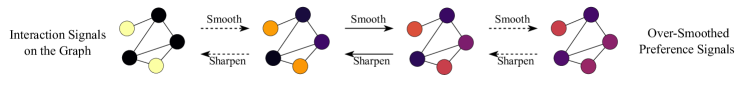
(b) Graph-aware diffusion in our GiffCF

Figure 1: Comparison of different diffusion processes for implicit feedback data.

In this paper, we focus on the potential application of conditional Diffusion Model (DM). By combining stepwise denoising with conditioning mechanisms, DMs have made remarkable success in various inverse problems in different domains, such as image inpainting (Rombach et al., 2022), accelerated MRI (Chung and Ye, 2022), time series imputation (Tashiro et al., 2021), etc. The ability of DMs to represent complex distributions can be attributed to their hierarchical structure, which allows each sampling step to make informative updates towards different directions. However, we argue that the standard Gaussian diffusion may not be suitable for modeling implicit feedback, primarily due to two reasons: (1) Gaussian perturbation destroys personalized signals in interaction vectors, leading to intermediate variables that do not contribute to recommendation performance. (2) The isotropic noise schedule fails to consider item heterogeneity and overlook the rich structural information present in the interaction matrix.

To address the first issue, Wang et al. (2023) proposed to limit the variance of added noise. They modeled historical interaction vectors as the final state of forward diffusion, simultaneously applyed multiplicative dropout and additive Gaussian perturbation for training data augmentation, and thus consistently enhanced the robustness of DAE. Although they avoided perturbing interaction vectors into pure noise like in image synthesis, this corruption manner is still hard to interpret, and we did not observe its superiority in our preliminary experiments.

In order to better harness the generative capabilities of DMs for collaborative filtering, we first propose to view historical interaction vectors as a conditional input to the diffusion denoiser, which serves as additional control signals for hierarchical generation. This modeling technique allows us to decouple forward corruption from the dropout of user history, and to explore more flexible diffusion strategies that are tailored for the inductive bias of recommender systems. Specifically, inspired by graph convolutional networks and image blurring filters, we innovatively define the forward diffusion as a smoothing process of interaction signals on an item-item similarity graph. Then, the reverse diffusion can be seen as a personalized process that gradually sharpens preference signals guided by users’ historical interactions. Our graph smoothing filters are based on state-of-the-art graph signal processing methods for collaborative filtering and can be implemented efficiently with either sparse or low-rank matrix multiplication. We further show that this diffusion process can be equivalently characterized as an anisotropic Gaussian diffusion in the graph spectral domain, establishing both forward and reverse formulations. Our contributions can be summarized as follows:

1. We propose a conditional diffusion framework for collaborative filtering. To our best knowledge, this is the first work that applies conditional DMs to pure implicit feedback data.

2. We introduce a novel smoothing filter for forward diffusion, which leverages the graph structure of implicit feedback data. The forward process itself demonstrates decent performance in top-$K$ recommendation.

3. We design a linear denoiser that dynamically weights reconstructed preferences and historical interactions in the embedding space and empirically show its effectiveness in recovering masked feedback. Our Graph-Aware Diffusion Model for Collaborative Filtering (GiffCF) outperforms baselines by a large margin on one dataset.

2 Background

Conditional Gaussian diffusion.

DM has achieved state-of-the-art in many conditional generative tasks. Given an initial sample ${\bm{x}}_{0}$ from the data distribution $q({\bm{x}}_{0})$, the forward process of Gaussian diffusion is defined through an increasingly noisy sequence of random variables deviating from ${\bm{x}}_{0}$, written as

$${\bm{x}}_{t}=\alpha_{t}{\bm{x}}_{0}+\sigma_{t}\bm{{\epsilon}}_{t},\quad\bm{{\epsilon}}_{t}\sim{\mathcal{N}}(\bm{0},\bm{I}),\quad t=1,2,\dots,T,$$ (1)

i.e. $q({\bm{x}}_{t}|{\bm{x}}_{0})={\mathcal{N}}({\bm{x}}_{t};\alpha_{t}{\bm{x}}_{0},\sigma_{t}^{2}\bm{I})$. In DDPM Ho et al. (2020), a variance-preserving noise schedule ensures that, while the noise level $\sigma_{t}$ monotonically increases from 0 to 1, its corresponding $\alpha_{t}$ decreases under the constraint $\alpha_{t}^{2}+\sigma_{t}^{2}=1$. In view of hierarchical generation, we care about how ${\bm{x}}_{s}$ and ${\bm{x}}_{t}$ from two arbitrary timesteps transition to each other. Thus, we split the noise term $\bm{{\epsilon}}_{s}=\sqrt{\sigma_{s}^{2}-\sigma_{s|t}^{2}}\bm{{\epsilon}}_{t}+\sigma_{s|t}\bm{{\epsilon}}_{s|t}$ and write $q({\bm{x}}_{s}|{\bm{x}}_{t},{\bm{x}}_{0})={\mathcal{N}}({\bm{x}}_{s};\alpha_{s}{\bm{x}}_{0}+\sqrt{\sigma_{s}^{2}-\sigma_{s|t}^{2}}\bm{{\epsilon}}_{t},\sigma_{s|t}^{2}\bm{I})$, where the variance $\sigma_{s|t}^{2}$ depends on further assumption. For instance, Ho et al. (2020) assumed the Markov property of forward process, leading to $\sigma_{t|s}^{2}=\sigma_{t}^{2}-\frac{\alpha_{t}^{2}\sigma_{s}^{2}}{\alpha_{s}^{2}}$ and $\sigma_{s|t}^{2}=\sigma_{s}^{2}-\frac{\alpha_{t}^{2}\sigma_{s}^{4}}{\alpha_{s}^{2}\sigma_{t}^{2}},\,\forall s<t$.To estimate the conditional distribution $q({\bm{x}}_{0}|{\bm{c}})$, we define the reverse process as a parameterized hierarchical model $p_{\theta}({\bm{x}}_{0}|{\bm{c}})=\int p({\bm{x}}_{T}|{\bm{c}})\prod_{t=1}^{T}p_{\theta}({\bm{x}}_{t-1}|{\bm{x}}_{t},{\bm{c}})\mathrm{d}{\bm{x}}_{1:T}$, letting $p({\bm{x}}_{T}|{\bm{c}})={\mathcal{N}}({\bm{x}}_{T};\bm{0},\bm{I})$, $p_{\theta}({\bm{x}}_{t-1}|{\bm{x}}_{t},{\bm{c}})=q({\bm{x}}_{t-1}|{\bm{x}}_{t},{\bm{x}}_{0}=\hat{{\bm{x}}}_{\theta}({\bm{x}}_{t},{\bm{c}},t))$ for $t=2,\dots,T$, and $p_{\theta}({\bm{x}}_{0}|{\bm{x}}_{1},{\bm{c}})={\mathcal{N}}({\bm{x}}_{0};\hat{{\bm{x}}}_{\theta}({\bm{x}}_{1},{\bm{c}},1)),\sigma_{0|1}^{2}\bm{I})$. The remaining task is to learn a neural denoiser $\hat{{\bm{x}}}_{\theta}$ via maximum likelihood estimation. During sampling, we start from a random noise ${\bm{x}}_{T}\sim p({\bm{x}}_{T})$, iteratively refine the noisy latent ${\bm{x}}_{t}$ by drawing ${\bm{x}}_{t-1}\sim p_{\theta}({\bm{x}}_{t-1}|{\bm{x}}_{t},{\bm{c}})$ for all $t=T,\dots,1$, and arrive at a final denoised sample ${\bm{x}}_{0}$.

Collaborative filtering as an inverse problem.

Next, let us consider collaborative filtering with implicit feedback, a common yet crucial senario in recommender systems. We denote the set of users as ${\mathcal{U}}$ and the set of items as ${\mathcal{I}}$. Our supervision is a user-item interaction matrix ${\bm{X}}\in\{0,1\}^{|{\mathcal{U}}|\times|{\mathcal{I}}|}$ with each row ${\bm{x}}_{u}\in\{0,1\}^{|{\mathcal{I}}|}$ representing the interaction vector of user $u$. The user has interacted with item $i$ if $x_{u,i}=1$, whereas no such interaction has been observed if $x_{u,i}=0$. For recommendation, we predict a preference score vector $\hat{{\bm{s}}}\in\mathbb{R}^{|{\mathcal{I}}|}$ to rank all the items, and then select top-$K$ potential items with no observed interactions but the highest scores. The difficulty we encounter here is that, the true score vector ${\bm{s}}$ are not explicitly available from the binary entries of ${\bm{X}}$. To address this issue, Wu et al. (2016) first proposed a self-supervised learning approach. Given an original interaction vector ${\bm{x}}$, they randomly dropped out each of its components to obtain an degraded version ${\bm{c}}$. Then, they trained an AE to invert ${\bm{c}}$ back to ${\bm{x}}$, minimizing a point-wise loss such as square error. At inference time, they inverted $u$’s historical interactions ${\bm{x}}_{u}$ to obtain its preference scores $\hat{{\bm{s}}}$. In this way, they essentially modeled the expectation $\mathbb{E}[{\bm{x}}|{\bm{c}}={\bm{x}}_{u}]$ as the ground-truth ${\bm{s}}$. Similarly, Liang et al. (2018) learned a multinomial $p({\bm{x}}|{\bm{c}})$ by means of variational Bayes, yielding a strong generative baseline known as Mult-VAE. These works both viewed recommendation as an ill-posed inverse problem; that is, user history ${\bm{c}}$ was degraded from ${\bm{x}}$ by a non-invertible forward operator, e.g. dropout. In this case, a deterministic recovery of ${\bm{x}}$ is thought to be unreliable. A more robust solution is to estimate $q({\bm{x}}|{\bm{c}})$, introducing probabilistic constraints for regularization. This is exactly the point where generative neural models like VAE and DM come into play.

A note on unconditional DM.

Before diving into our method, we point out that unconditional DM can be used to solve a certain kind of inverse problem. For example, Wang et al. (2023) assumed an intrinsic Gaussian noise present in each ${\bm{x}}_{u}$. In their DiffRec, interactions for user $u$ were reconstructed from $p_{\theta}({\bm{x}}_{0}|{\bm{x}}_{T}={\bm{x}}_{u})$, where ${\bm{x}}_{T}$ is the final state defined by Equation 1, but with a small-scale noise ($\sigma_{T}\ll 1$). Notably, they still employed a large dropout rate for all the latents ${\bm{x}}_{t}$ during training. In contrast, a conditional DM for collaborative filtering performs dropout and forward diffusion to ${\bm{c}}$ and ${\bm{x}}_{t}$ respectively, resulting in a fundamentally distinct inference model (Figure 2(b)).

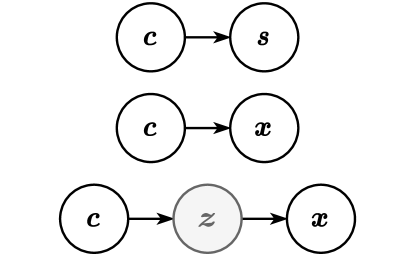
(a) Non-diffusion recommender models. Instead of directly predicting scores ${\bm{s}}$ (top), DAE and VAE (middle or bottom) learn to generate interactions ${\bm{x}}$.

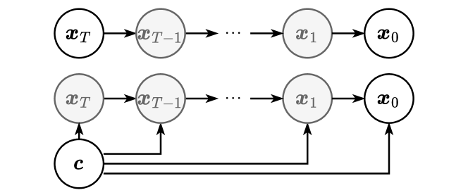
(b) Diffusion recommender models. Recent works studied unconditional DMs for collaborative filtering (top). We propose conditional modeling of historical interactions ${\bm{c}}$ (bottom).

Figure 2: Graphical models for different recommender models at inference time. Latent variables are colored in gray.

3 Collaborative Forward Process

While conventional DMs rely on Gaussian perturbation to effectively explore the distribution of pixel data, recent works have shown that this forward corruption manner is not unique (Daras et al., 2022; Bansal et al., 2022). To better leverage the hierarchical structure of DM for collaborative filtering, we are interested in finding a diffusion strategy specialized for implicit feedback data.

3.1 Graph Smoothing with Heat Equation

To begin with, we observe that just as an image can be seen as a signal on a two-dimensional lattice of pixels, a user’s interaction vector can be considered a signal on an item-item similarity graph. Inspired by the over-smoothing artifact in GNNs (Rusch et al., 2023), we immediately notice a corruption manner applicable to graph signals: repeating smoothing operations until it reaches a steady state. Interestingly, similar attempts using blurring filters for forward diffusion have been made in image synthesis literature (Rissanen et al., 2022; Hoogeboom and Salimans, 2023). The general idea of a smoothing process is to progressively exchange information on a (discretized) Riemanian manifold (e.g., an item-item graph), which is well described by the following partial differential equation in continuous time:

$$\frac{\partial{\bm{x}}}{\partial\tau}=\alpha\nabla^{2}{\bm{x}},$$ (2)

known as the heat equation. Intuitively, the Laplacian operator $\nabla^{2}$ measures the information difference between a point and the average of its neighborhood, and $\alpha$ captures the rate at which information is exchanged over time $\tau$. In the case of interaction signals, we define $\nabla^{2}={\bm{A}}-{\bm{I}}$ by convention, where ${\bm{A}}$ is a normalized adjacency matrix of the item-item graph. It is straightforward to verify the closed form solution of Equation 2 given some initial value ${\bm{x}}(0)$:

$${\bm{x}}(\tau)=\exp\{-\tau\alpha({\bm{I}}-{\bm{A}})\}{\bm{x}}(0)={\bm{U}}\exp\{-\tau\alpha(\bm{1}-\bm{\lambda})\}\odot{\bm{U}}^{\top}{\bm{x}}(0),\quad\tau\geq 0,$$ (3)

where ${\bm{U}}=[{\bm{u}}_{1},\dots,{\bm{u}}_{|{\mathcal{I}}|}]$ is the matrix of unit eigenvectors of ${\bm{A}}$, the corresponding eigenvalues $\bm{\lambda}=[\lambda_{1},\dots,\lambda_{|{\mathcal{I}}|}]$ are sorted in descending order, and $\odot$ denotes Hadamard product. The orthonormal matrix ${\bm{U}}^{\top}$ is often referred to as graph Fourier transform (GFT) matrix and ${\bm{U}}$ as its inverse, and the eigenvalues of $-\nabla^{2}$, i.e. $\bm{1}-\bm{\lambda}$, are called graph frequencies (Chung, 1997). Thus, Equation 3 can be interpreted as exponentially decaying each high-frequency component of the interaction signal ${\bm{x}}$ with a different rate $\alpha(\bm{1}-\bm{\lambda})$. As $\tau\to+\infty$, the signal ${\bm{x}}(\tau)$ converges to a over-smoothed steady state ${\bm{x}}(+\infty)={\bm{u}}_{1}{\bm{u}}_{1}^{\top}{\bm{x}}(0)$.

A problem of this smoothing process is that, it is computationally intractable to find the matrix exponential or fully diagonalize ${\bm{A}}$ for real-world item-item graphs with thousands and millions of nodes. One solution is to approximate the continuous-time filter in Equation 3 using its first-order Taylor expansion with respect to $\tau$:

$$\exp\{-\tau\alpha({\bm{I}}-{\bm{A}})\}=(1-\tau\alpha){\bm{I}}+\tau\alpha{\bm{A}}+{\mathcal{O}}(\tau).$$ (4)

While it is possible to numerically solve Equation 2 with Euler method, here we simply set $\tau=1$ for our final state and linearly interpolate the intermediate states to avoid computational overhead, obtaining a sequence of forward filters

$${\bm{F}}_{t}=(1-\tau_{t}\alpha){\bm{I}}+\tau_{t}\alpha{\bm{A}},\quad t=0,1,2,\dots,T,$$ (5)

where $0=\tau_{0}<\tau_{1}<\dots<\tau_{T}=1$ defines a smoothing schedule. Note that by first-order truncation, we only consider 1-hop propogation of message on the item-item graph.

Unlike the standard Gaussian diffusion that adds noise and destructs useful signals, our smoothing filters have the capability to reduce noise and introduce structural information of the item-item graph, which potentially benefits recommendation and coincides with the idea of graph signal processing techniques for collaborative filtering (Shen et al., 2021; Fu et al., 2022; Choi et al., 2023). These prior works also offer insights into how to construct the item-item adjacency matrix ${\bm{A}}$, which we will discuss in Section 3.2.

3.2 Identifying the Item-Item Graph

The interaction matrix ${\bm{X}}$ provides the adjacency between a user node and an item node on the user-item bipartite graph, yet to smooth an interaction vector, it is necessary to measure the similarity between two item nodes. Let us define ${\bm{D}}_{\mathcal{U}}=\mathrm{diagMat}({\bm{X}}\bm{1})$ and ${\bm{D}}_{\mathcal{I}}=\mathrm{diagMat}({\bm{X}}^{\top}\bm{1})$ as the degree matrices of users and items, respectively. A popular approach to construct an adjacency matrix for the item-item graph is to stack two convolution kernels $\tilde{{\bm{A}}}_{\rm LGN}$ proposed in LightGCN (He et al., 2020):

$$\tilde{{\bm{A}}}_{\rm LGN}^{2}=\begin{bmatrix}{\bm{O}}&{\bm{D}}_{\mathcal{U}}^{-\frac{1}{2}}{\bm{X}}{\bm{D}}_{\mathcal{I}}^{-\frac{1}{2}}\\ {\bm{D}}_{\mathcal{I}}^{-\frac{1}{2}}{\bm{X}}^{\top}{\bm{D}}_{\mathcal{U}}^{-\frac{1}{2}}&{\bm{O}}\end{bmatrix}^{2}=\begin{bmatrix}{\bm{D}}_{\mathcal{U}}^{-\frac{1}{2}}{\bm{X}}{\bm{D}}_{\mathcal{I}}^{-1}{\bm{X}}^{\top}{\bm{D}}_{\mathcal{U}}^{-\frac{1}{2}}&{\bm{O}}\\ {\bm{O}}&{\bm{D}}_{\mathcal{I}}^{-\frac{1}{2}}{\bm{X}}^{\top}{\bm{D}}_{\mathcal{U}}^{-1}{\bm{X}}{\bm{D}}_{\mathcal{I}}^{-\frac{1}{2}},\end{bmatrix}$$ (6)

and then use the lower-right block, which we denote by ${\bm{A}}_{\frac{1}{2},1,\frac{1}{2}}$. On the other hand, Fu et al. (2022) proposed a more general form of link propagation on the bipartite graph. Here, we reformulate it as an item-item matrix

$${\bm{A}}_{\beta,\gamma,\delta}={\bm{D}}_{\mathcal{I}}^{-\delta}{\bm{X}}^{\top}{\bm{D}}_{\mathcal{U}}^{-\gamma}{\bm{X}}{\bm{D}}_{\mathcal{I}}^{-\beta},$$ (7)

where $\beta,\gamma,\delta$ are parameters to be tuned. When $\beta=\gamma=\delta=0$, the similarity measure degrades into the number of common neighbors between two item nodes (Newman, 2001). The importance of normalization lies in that, nodes with higher degrees often contain less information about their neighbors, and thus should be down-weighted. Empirically, we find that ${\bm{A}}_{\frac{1}{2},\frac{1}{2},\frac{1}{2}}$ consistently performs better than ${\bm{A}}_{\frac{1}{2},1,\frac{1}{2}}$, so it serves as our default choice.

Nevertheless, this filter still only aggregates information from 2-hop neighbors on the original bipartite graph. Breaking this limitation, Shen et al. (2021) propose to strengthen it with a ideal low-pass filter. Basically, if we denote ${\bm{U}}_{\beta,\gamma,\delta,d}$ as the matrix of eigenvectors corresponding to the top-$d$ eigenvalues of ${\bm{A}}_{\beta,\gamma,\delta}$ (lowest $d$ graph frequencies), the low-pass filter can be decomposed as ${\bm{U}}_{\beta,\gamma,\delta,d}{\bm{U}}_{\beta,\gamma,\delta,d}^{\top}$. Multiplying it with an interaction vector ${\bm{x}}$ filters out high-frequency components while preserving dense, high-order signals in the low-frequency subspace. We summarize representative collaborative filtering techniques related to graph filters in Table 1. Integrating the designs of LinkProp and GF-CF, we propose the following item-item adjacency matrix for our forward filters:

$${\bm{A}}=\frac{1}{1+w}{\bm{A}}_{\frac{1}{2},\frac{1}{2},\frac{1}{2}}/\|{\bm{A}}_{\frac{1}{2},\frac{1}{2},\frac{1}{2}}\|_{2}+\frac{w}{1+w}{\bm{U}}_{\frac{1}{2},\frac{1}{2},\frac{1}{2},d}{\bm{U}}_{\frac{1}{2},\frac{1}{2},\frac{1}{2},d}^{\top},$$ (8)

where $d$ and $w$ are the cut-off dimension and the strength of ideal low-pass filtering, respectively. Note that the resulting matrix has been scaled to unit norm. The truncated eigendecomposition can be implemented in a preprocessing stage using iterative (Baglama and Reichel, 2005) or randomized (Musco and Musco, 2015) algorithms efficiently. In the forward process, the link propagation term requires sparse matrix multiplication and costs ${\mathcal{O}}(|{\mathcal{X}}|)$ time for each ${\bm{x}}$, where $|{\mathcal{X}}|$ is the number of observed interactions in the training data; the ideal low-pass term requires low-rank matrix multiplication and costs ${\mathcal{O}}(|{\mathcal{I}}|d)$ time. Both of them sidestep the need for ${\mathcal{O}}(|{\mathcal{I}}|^{2})$ dense multiplication.

Table 1: A summary of graph filters for interaction signals. ${\bm{x}}$ denotes input and ${\bm{y}}$ denotes output. Scaling factors that do not affect top-$K$ recommendation results are omitted. ^†We use Euler method, single blurring/sharpening steps and early merge in BSPM to simplify its notation for clear comparison.

Method	Formulation	Parameters
Low-rank linear AE	${\bm{y}}={\bm{W}}_{\rm dec}{\bm{W}}_{\rm enc}{\bm{x}}$	${\bm{W}}_{\rm enc}\in\mathbb{R}^{|{\mathcal{I}}|\times d}$, ${\bm{W}}_{\rm dec}\in\mathbb{R}^{d\times|{\mathcal{I}}|}$
2-layer AE (MLP)	${\bm{y}}={\bm{W}}_{\rm dec}\tanh({\bm{W}}_{\rm enc}{\bm{x}}+{\bm{b}}_{\rm enc})+{\bm{b}}_{\rm dec}$	${\bm{b}}_{\rm enc}\in\mathbb{R}^{d}$, ${\bm{b}}_{\rm dec}\in\mathbb{R}^{|{\mathcal{I}}|}$
LinkProp (Fu et al., 2022)	${\bm{y}}={\bm{A}}_{\beta,\gamma,\delta}{\bm{x}}$	Equation 7
GF-CF (Heat equation)	${\bm{y}}={\bm{A}}_{\rm HE}{\bm{x}}$	${\bm{A}}_{\rm HE}={\bm{A}}_{\frac{1}{2},1,\frac{1}{2}}$
GF-CF (Ideal low-pass)	${\bm{y}}={\bm{A}}_{\rm IDL}{\bm{x}}$	${\bm{A}}_{\rm IDL}={\bm{D}}_{\mathcal{I}}^{\frac{1}{2}}{\bm{U}}_{\frac{1}{2},1,\frac{1}{2},d}{\bm{U}}_{\frac{1}{2},1,\frac{1}{2},d}^{\top}{\bm{D}}_{\mathcal{I}}^{-\frac{1}{2}}$
GF-CF (Shen et al., 2021)	${\bm{y}}=({\bm{A}}_{\rm HE}+w{\bm{A}}_{\rm IDL}){\bm{x}}$	$w\geq 0$
BSPM† (Choi et al., 2023)	${\bm{y}}=({\bm{I}}-w_{2}{\bm{A}}_{\rm HE})({\bm{A}}_{\rm HE}+w_{1}{\bm{A}}_{\rm IDL}){\bm{x}}$	$w_{1},w_{2}\geq 0$
GiffCF forward (Ours)	${\bm{y}}=({\bm{A}}_{\frac{1}{2},\frac{1}{2},\frac{1}{2}}/\|{\bm{A}}_{\frac{1}{2},\frac{1}{2},\frac{1}{2}}\|_{2}+w{\bm{U}}_{\frac{1}{2},\frac{1}{2},\frac{1}{2},d}{\bm{U}}_{\frac{1}{2},\frac{1}{2},\frac{1}{2},d}^{\top}){\bm{x}}$

3.3 Diffusion in the Graph Spectral Domain

So far, we have introduced a deterministic corruption manner for interaction signals but ignored the probabilistic modeling aspect of DM. For the sake of robust learning, it is reasonable to add Gaussian noise while applying smoothing filters. Hence, our full collaborative forward process is given by

$${\bm{x}}_{t}={\bm{F}}_{t}{\bm{x}}_{0}+\sigma_{t}\bm{{\epsilon}}_{t},\quad\bm{{\epsilon}}_{t}\sim{\mathcal{N}}(\bm{0},\bm{I}),\quad t=0,1,2,\dots,T,$$ (9)

where $({\bm{F}}_{t})_{t=1}^{T}$ is defined in Equation 5 and $(\sigma_{t})_{t=1}^{T}$ controls the noise level. Comparing it with Equation 1, we can see that the mere difference between standard forward diffusion and ours lies in the choice of ${\bm{F}}_{t}$: the former uses a diagonal matrix ${\bm{F}}_{t}=\alpha_{t}{\bm{I}}$, while we adopt a graph-aware dense matrix leveraging collaborative signals from implicit feedback data. To give a further correspondence between the two processes, we diagonalize our filters as

$${\bm{F}}_{t}={\bm{U}}[(1-\tau_{t}\alpha)\bm{1}+\tau_{t}\alpha\bm{\lambda}]\odot{\bm{U}}^{\top},\quad t=0,1,2,\dots,T,$$ (10)

Note that ${\bm{F}}_{t}$, ${\bm{A}}$ and ${\bm{A}}_{\frac{1}{2},\frac{1}{2},\frac{1}{2}}$ share the same orthonormal matrix ${\bm{U}}$ of eigenvectors. After writing the GFT of ${\bm{x}}_{t}$ as $\tilde{{\bm{x}}}_{t}={\bm{U}}^{\top}{\bm{x}}_{t}$ and the GFT of $\bm{{\epsilon}}_{t}$ as $\tilde{\bm{{\epsilon}}}_{t}={\bm{U}}^{\top}\bm{{\epsilon}}_{t}$, we plug Equation 10 into Equation 9 and obtain an equivalent formulation of our forward process in the graph spectral domain:

$$\tilde{{\bm{x}}}_{t}=[(1-\tau_{t}\alpha)\bm{1}+\tau_{t}\alpha\bm{\lambda}]\odot\tilde{{\bm{x}}}_{0}+\sigma_{t}\tilde{\bm{{\epsilon}}}_{t},\quad\tilde{\bm{{\epsilon}}}_{t}\sim{\mathcal{N}}(\bm{0},\bm{I}),\quad t=0,1,2,\dots,T.$$ (11)

It turns out to be a special case of Gaussian diffusion with an anisotropic noise schedule; that is, the scalar multiplier $\alpha_{t}$ in Equation 1 now becomes a vector $\bm{\alpha}_{t}=(1-\tau_{t}\alpha)\bm{1}+\tau_{t}\alpha\bm{\lambda}$. We illustrate such schedule in Figure 3.

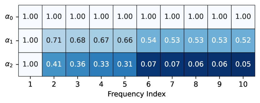
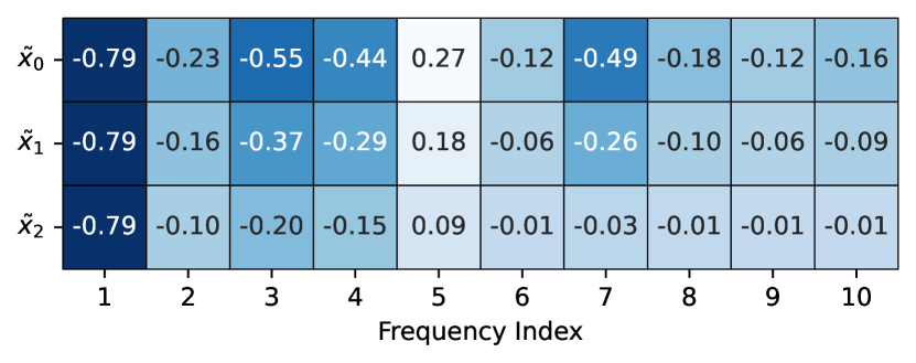
Figure 3: An example of anisotropic $\bm{\alpha}_{t}$ with $d=5$, $w=0.3$, $\alpha=1$, $T=2$ and linear smoothing schedule.

4 Personalized Reverse Process

The collaborative forward process smooths the interactions ${\bm{x}}_{0}$ of an individual, transforming it into preference scores that reflect common interests among all the users. As its counterpart, we expect a personalized reverse process to sharpen the preferences ${\bm{x}}_{T}$, recovering user idiosyncrasies under the guidance of historical interactions ${\bm{c}}$. From the perspective of generative modeling, Equation 9 defines a sequence of latent variables with fixed variational distributions $q({\bm{x}}_{t}|{\bm{x}}_{0})={\mathcal{N}}({\bm{x}}_{t};{\bm{F}}_{t}{\bm{x}}_{0},\sigma_{t}^{2}{\bm{I}})$, which enables us to learn a posterior distribution $p_{\theta}({\bm{x}}_{0}|{\bm{x}}_{T},{\bm{c}})=\prod^{T}_{t=1}p_{\theta}({\bm{x}}_{t-1}|{\bm{x}}_{t},{\bm{c}})$ as a Markov chain for generating new samples of ${\bm{x}}_{0}$.

4.1 Generalized Diffusion Loss

Specifically, we aim to maximize the conditional log-likelihood of the generated data:

$$\log p_{\theta}({\bm{x}}_{0}|{\bm{c}}) =\log\mathbb{E}_{q({\bm{x}}_{1:T}|{\bm{x}}_{0})}\left[\frac{p_{\theta}({\bm{x}}_{0:T}|{\bm{c}})}{q({\bm{x}}_{1:T}|{\bm{x}}_{0})}\right]\geq\mathbb{E}_{q({\bm{x}}_{1:T}|{\bm{x}}_{0})}\left[\log\frac{p_{\theta}({\bm{x}}_{0:T}|{\bm{c}})}{q({\bm{x}}_{1:T}|{\bm{x}}_{0})}\right]$$ (12)

$$=-\underbrace{D_{\mathrm{KL}}\left(q({\bm{x}}_{T}|{\bm{x}}_{0})\parallel p({\bm{x}}_{T}|{\bm{c}})\right)}_{\mathcal{L}_{T}}-\underbrace{\mathbb{E}_{q({\bm{x}}_{1}|{\bm{x}}_{0})}\left[-\log p_{\theta}({\bm{x}}_{0}|{\bm{x}}_{1},{\bm{c}})\right]}_{\mathcal{L}_{0}}$$

$$\quad-\sum^{T}_{t=2}\underbrace{\mathbb{E}_{q({\bm{x}}_{t}|{\bm{x}}_{0})}\left[D_{\mathrm{KL}}\left(q({\bm{x}}_{t-1}|{\bm{x}}_{t},{\bm{x}}_{0})\parallel p_{\theta}({\bm{x}}_{t-1}|{\bm{x}}_{t},{\bm{c}})\right)\right]}_{\mathcal{L}_{t-1}}.$$

The right-hand side of the above inequality is known as the evidence lower bound (ELBO) of the log-likelihood. In practice, we set $p({\bm{x}}_{T}|{\bm{c}})=q({\bm{x}}_{T}|{\bm{x}}_{0}={\bm{c}})$ (smoothing ${\bm{c}}$ to get ${\bm{x}}_{T}$) and ignore optimization of the prior term ${\mathcal{L}}_{T}$. For the other terms, similar to the isotropic diffusion introduced in Section 2, we first write $q({\bm{x}}_{s}|{\bm{x}}_{t},{\bm{x}}_{0})$ as ${\mathcal{N}}({\bm{x}}_{s};{\bm{F}}_{s}{\bm{x}}_{0}+\sqrt{\sigma_{s}^{2}-\sigma_{s|t}^{2}}\bm{{\epsilon}}_{t},\sigma_{s|t}^{2}\bm{I})$. Then, we parameterize $p_{\theta}({\bm{x}}_{t-1}|{\bm{x}}_{t},{\bm{c}})$ as $q({\bm{x}}_{t-1}|{\bm{x}}_{t},{\bm{x}}_{0}=\hat{{\bm{x}}}_{\theta}({\bm{x}}_{t},{\bm{c}},t))$ for $t=2,\dots,T$ and $p_{\theta}({\bm{x}}_{0}|{\bm{x}}_{1},{\bm{c}})$ as ${\mathcal{N}}({\bm{x}}_{0};\hat{{\bm{x}}}_{\theta}({\bm{x}}_{1},{\bm{c}},1),\sigma_{0|1}^{2}\bm{I})$, where $\hat{{\bm{x}}}_{\theta}$ is a neural denoiser to be learned. Under these Gaussian assumptions, we can now derive the closed-form solutions for the reconstruction term ${\mathcal{L}}_{0}$:

$${\mathcal{L}}_{0}=\mathbb{E}_{q({\bm{x}}_{1}|{\bm{x}}_{0})}\left[\frac{1}{2\sigma_{0|1}^{2}}\|\hat{{\bm{x}}}_{\theta}({\bm{x}}_{1},{\bm{c}},1)-{\bm{x}}_{0}\|^{2}\right]+C,$$ (13)

and for the denoising matching terms ${\mathcal{L}}_{t-1}$, $t=2,\dots,T$:

$${\mathcal{L}}_{t-1}=\mathbb{E}_{q({\bm{x}}_{t}|{\bm{x}}_{0})}\left[\frac{\left(\sigma_{t}-\sqrt{\sigma^{2}_{t-1}-\sigma^{2}_{t-1|t}}\right)^{2}}{2\sigma^{2}_{t}\sigma^{2}_{t-1|t}}\|{\bm{F}}_{t-1}\hat{{\bm{x}}}_{\theta}({\bm{x}}_{t},{\bm{c}},t)-{\bm{F}}_{t-1}{\bm{x}}_{0}\|^{2}\right].$$ (14)

Note that we can further relax Equation 14 using $\|{\bm{F}}_{t-1}\hat{{\bm{x}}}_{\theta}({\bm{x}}_{t},{\bm{c}},t)-{\bm{F}}_{t-1}{\bm{x}}_{0}\|\leq\|{\bm{F}}_{t-1}\|_{2}\|\hat{{\bm{x}}}_{\theta}({\bm{x}}_{t},{\bm{c}},t)-{\bm{x}}_{0}\|$. Therefore, the total loss reduces to a summation of $T$ weighted square errors. Following Ho et al. (2020), we sample the timestep $t$ uniformly at random and minimize a reweighted version of diffusion loss:

$${\mathcal{L}}=\mathbb{E}_{t\sim{\mathcal{U}}(1,T),q({\bm{x}}_{t}|{\bm{x}}_{0})}[w_{t}\|\hat{{\bm{x}}}_{\theta}({\bm{x}}_{t},{\bm{c}},t)-{\bm{x}}_{0}\|^{2}],$$ (15)

which is identical to the loss function for a standard DM. While DMs for image synthesis typically learn a U-Net (Ronneberger et al., 2015) image denoiser for predicting $\bm{{\epsilon}}_{t}$ and essentially set $w_{t}$ to the signal-to-noise ratio $\frac{\alpha_{t}^{2}}{\sigma_{t}^{2}}$ (Kingma et al., 2023), in this paper, we choose to predict ${\bm{x}}_{0}$ with $w_{t}=1$ for all $t=1,\dots,T$.

Input: Interaction matrix ${\bm{X}}$.

1 repeat

2       Sample $u$ from ${\mathcal{U}}$ and let ${\bm{x}}_{0}\leftarrow{\bm{x}}_{u}$.

3       Randomly mask out ${\bm{x}}_{0}$ to obtain ${\bm{c}}$.

4       Sample $t\sim{\mathcal{U}}(1,T)$ and ${\bm{x}}_{t}\sim{\mathcal{N}}({\bm{F}}_{t}{\bm{x}}_{0},\sigma_{t}^{2}\bm{I})$.

5       Take gradient step on $\|\hat{{\bm{x}}}_{\theta}({\bm{x}}_{t},{\bm{c}},t)-{\bm{x}}_{0}\|^{2}$.

6      

7until converged;

Output: Denoiser parameters $\theta$.

Algorithm 1 GiffCF training.

Input: $\theta$ and historical interactions ${\bm{x}}_{u}$

1 Let ${\bm{c}}\leftarrow{\bm{x}}_{u}$ and ${\bm{x}}_{T}\leftarrow{\bm{F}}_{T}{\bm{c}}$.

2 for $t=T,\dots,1$ do

3       Predict $\hat{{\bm{x}}}_{0}\leftarrow\hat{{\bm{x}}}_{\theta}({\bm{x}}_{t},{\bm{c}},t)$.

4       Compute $\hat{\bm{{\epsilon}}}_{t}\leftarrow({\bm{x}}_{t}-{\bm{F}}_{t}\hat{{\bm{x}}}_{0})/\sigma_{t}$.

5       Update ${\bm{x}}_{t-1}\leftarrow{\bm{F}}_{t-1}\hat{{\bm{x}}}_{0}+\sigma_{t-1}\hat{\bm{{\epsilon}}}_{t}$.

6      

7 end for

Output: Reconstructed preferences ${\bm{x}}_{0}$.

Algorithm 2 GiffCF inference.

4.2 Sampling with the Preference Denoiser

Since our ultimate goal is to achieve higher accuracy for top-$K$ recommendation, we contend that uncertainty should not be present in the sampling steps. Thus, we follow the sampler of DDIM (Song et al., 2022) and assume $\sigma_{t-1|t}^{2}=0$ for all $p_{\theta}({\bm{x}}_{t-1}|{\bm{x}}_{t})$, $t=1,\dots,T$. The resulting reverse process then becomes a deterministic mapping from ${\bm{x}}_{T}$ to ${\bm{x}}_{0}$.

On the design of $\hat{x}_{\theta}$, we adopt a simplistic linear AE as our backbone and implement conditioning as a dynamic weighted aggregation of ${\bm{x}}_{t}$ and ${\bm{c}}$ in the embedding space. Despite its simplicity, we find that this preference denoiser is not only effective but also interpretable. The network architecture can be summarized by the following equation:

$$\hat{x}_{\theta}({\bm{x}}_{t},{\bm{c}},t)={\bm{W}}^{\top}\mathrm{Dropout}\left(\theta_{1}(t){\bm{W}}\frac{{\bm{x}}_{t}}{\|{\bm{c}}\|}+\theta_{2}(t){\bm{W}}\frac{{\bm{c}}}{\|{\bm{c}}\|}\right),$$ (16)

Here, ${\bm{W}}\in\mathbb{R}^{d\times|{\mathcal{I}}|}$ is the shared weight matrix of encoder and decoder, which may be viewed as a set of item embeddings. $\theta_{1}(t)$ and $\theta_{2}(t)$ are two learnable scalar functions of the timestep $t$ on the sinusoidal basis. We use $L^{2}$ normalization on the input and an additional dropout before the decoder layer to prevent overfitting.

The full training and inference procedures of GiffCF are summarized in Algorithm 1 and Algorithm 2, respectively. In our implementation, we use a linear smoothing schedule with $\tau_{t}=t/T$, $t=0,1,\dots,T$ and a constant noise schedule with $\sigma_{t}\equiv\sigma$, $t=0,1,\dots,T$ (Note that we include $\sigma_{0}$), simplifying each iteration in Algorithm 2 to

$${\bm{x}}_{t-1}={\bm{x}}_{t}-\frac{1}{T}({\bm{I}}-{\bm{A}})\hat{{\bm{x}}}_{\theta}({\bm{x}}_{t},{\bm{c}},t).$$ (17)

As can be seen, the implemented reverse process iteratively removes the predicted difference between the initial and smoothed interaction signals, aligning with our intuition of sharpening the preferences.

5 Experiments

In this section, we conduct experiments on three real-world datasets to verify the effectiveness of GiffCF. We aim to answer the following research questions:

• How does GiffCF perform compared to state-of-the-art baselines, especially diffusion-based recommender models and graph signal processing techniques?

• How does the smoothing schedule (controlled by $\alpha$), the noise schedule (controlled by $\sigma$) and the number of diffusion steps $T$ affect the performance of GiffCF?

• How does the preference denoiser, particularly the dynamic weighting mechanism, behave during sampling?

5.1 Experimental Setup

For a fair comparison, we use the same preprocessed and split versions of three public datasets as in Wang et al. (2023):

• MovieLens-1M contains 571,531 interactions among 5,949 users and 2,810 items with a sparsity of 96.6%.

• Yelp contains 1,402,736 interactions among 54,574 users and 34,395 items with a sparsity of 99.93%.

• Amazon-Book contains 3,146,256 interactions among 108,822 users and 94,949 items with a sparsity of 99.97%.

Each dataset is split into training, validation, and testing sets with a ratio of 7:1:2. For each trainable method, we use the validation set to select the best epoch and the testing set to obtain the final results and tune the hyper-parameters. To evaluate the top-$K$ recommendation performance, we report the average Recall@$K$ (normalized as in Liang et al. (2018)), NDCG@$K$ and MRRecall@$K$ among all the users. The following baseline methods are considered:

• MF (Koren et al., 2009) & LightGCN (He et al., 2020), two of the most representative recommender models that optimize BPR loss (Rendle et al., 2012). The latter linearly aggregates user/item embeddings on the bipartite graph.

• Mult-VAE (Liang et al., 2018), which generates interaction vectors from its underlying multinomial distribution.

• DiffRec & L-DiffRec (Wang et al., 2023), unconditional diffusion recommender models with standard Gaussian diffusion. The latter variant perturbs the latent representation of an interaction vector encoded by multiple VAEs.

• LinkProp (Fu et al., 2022) & BSPM (Choi et al., 2023), state-of-the-art graph signal processing techniques for collaborative filtering (Table 1), which significantly outperform embedding-based models on large, sparse datasets.

Table 2: Performance comparison on all three datasets. The best results are highlighted in bold and the second-best results are underlined. %Improv. represents the relative improvements of GiffCF over the best baseline results. * implies the improvements over the best baseline are statistically significant ($p$-value $<0.05$) under one-sample t-tests.

(a) Results on MovieLens-1M.

Method	Recall@10	Recall@20	NDCG@10	NDCG@20	MRR@10	MRR@20
MF	0.0885	0.1389	0.0680	0.0871	0.1202	0.1325
LightGCN	0.1112	0.1798	0.0838	0.1089	0.1363	0.1495
Mult-VAE	0.1170	0.1833	0.0898	0.1149	0.1493	0.1616
DiffRec	0.1178	0.1827	0.0901	0.1148	0.1507	0.1630
L-DiffRec	0.1174	0.1847	0.0868	0.1122	0.1394	0.1520
LinkProp	0.1039	0.1509	0.0852	0.1031	0.1469	0.1574
BSPM	0.1107	0.1740	0.0838	0.1079	0.1388	0.1513
GiffCF	0.1275∗	0.1942∗	0.0999∗	0.1250∗	0.1625∗	0.1747∗
%Improv.	8.23%	5.14%	10.88%	8.79%	7.83%	7.18%

(b) Results on Yelp.

Method	Recall@10	Recall@20	NDCG@10	NDCG@20	MRR@10	MRR@20
MF	0.0509	0.0852	0.0301	0.0406	0.0354	0.0398
LightGCN	0.0629	0.1041	0.0379	0.0504	0.0446	0.0497
Mult-VAE	0.0595	0.0979	0.0360	0.0477	0.0425	0.0474
DiffRec	0.0586	0.0961	0.0363	0.0487	0.0445	0.0493
L-DiffRec	0.0589	0.0971	0.0353	0.0469	0.0411	0.0460
LinkProp	0.0604	0.0980	0.0370	0.0485	0.0445	0.0493
BSPM	0.0630	0.1033	0.0382	0.0505	0.0452	0.0503
GiffCF	0.0631	0.1035	0.0387	0.0509	0.0464	0.0514
%Improv.	0.16%	-	1.31%	0.79%	2.65%	2.19%

(c) Results on Amazon-Book.

Method	Recall@10	Recall@20	NDCG@10	NDCG@20	MRR@10	MRR@20
MF	0.0686	0.1037	0.0414	0.0518	0.0430	0.0471
LightGCN	0.0699	0.1083	0.0421	0.0536	0.0443	0.0487
Mult-VAE	0.0688	0.1005	0.0424	0.0520	0.0455	0.0482
DiffRec	0.0700	0.1011	0.0451	0.0547	0.0502	0.0540
L-DiffRec	0.0697	0.1029	0.0440	0.0540	0.0468	0.0506
LinkProp	0.1087	0.1488	0.0709	0.0832	0.0762	0.0807
BSPM	0.1055	0.1435	0.0696	0.0814	0.0763	0.0808
GiffCF	0.1089	0.1490	0.0710	0.0833	0.0762	0.0808
%Improv.	0.18%	0.13%	0.14%	0.12%	-	-

For DiffRec and L-DiffRec, we reuse the checkpoints released by the authors, which are tuned in a vast search space. For the other baselines, we set all the user/item embedding sizes, hidden layer sizes, cut-off dimension of ideal low-pass filters to 200. In specific, the architecture of Mult-VAE will become $[|{\mathcal{I}}|,200,200,200,|{\mathcal{I}}|]$ including the input and output layers. The dropout rates for generative recommender models are set to 0.5. Hyper-parameters not mentioned above are tuned or set to the default values suggested by the authors. For our own model, by default, we set $T=3$ as the number of diffusion steps, $\alpha=1.5$ for the smoothing schedule, and tune the noise scale $\sigma$ in $\{0.0,0.05,0.1,0.15,0.2\}$, the ideal low-pass filters weight $w$ in $\{0.0,0.1,0.2,0.3,0.4,0.5\}$. We optimize all the models using Adam (Kingma and Ba, 2017) with a constant learning rate in $\{10^{-5},10^{-4},10^{-3}\}$ and apply no weight decay. More details will be present in our released code.

5.2 Comparison with the State-of-the-Art

The overall performance of GiffCF and the baselines on all three datasets is shown in Table 2. (1) We can see that GiffCF consistently outperforms all the baselines on MovieLens-1M, yielding an impressive improvement on all the metrics. (2) On the two sparse datasets, Yelp and Amazon-Book, the improvements seems to be less significant but still comparable to the best baselines, especially the graph signal processing techniques.

These results indicate that the preference denoiser suffers from the common bottleneck among embedding-based models and fails to predict ${\bm{x}}_{0}$ precisely when the number of items is large. While our item-item adjacency matrix ${\bm{A}}$ in the forward filters is designed to improve upon LinkProp and GF-CF and handles the sparsity issue well, GiffCF may probably learn to preserve the smoothed results ${\bm{x}}_{T}$ from the forward process, limiting the impact of the reverse sharpening. We will show more evidence in Section 5.4.

5.3 Sensitivity Analysis

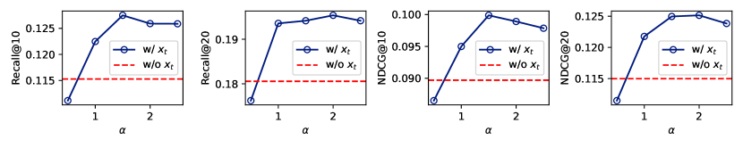
(a) Sensitivity on $\alpha$.

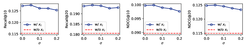
(b) Sensitivity on $\sigma$.

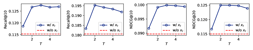
(c) Sensitivity on $T$.

Figure 4: Performance of GiffCF on MovieLens-1M with different values of $\alpha$, $\sigma$ and $T$.

We perform sensitivity analysis on MovieLens-1M, which best showcases the power of GiffCF. To demonstrate the effect of graph-aware diffusion, we compare our model with a condition-only model whose denoiser do not take ${\bm{x}}_{t}$ as input (w/o ${\bm{x}}_{t}$ in the plots). (1) From Figure 4(a), we see that the smoothing strength $\alpha$ has a considerable impact on the effectiveness of diffusion. When $\alpha$ is too small, the forward process only partially smoothed the interactions and the resulting diffusion latents mixed with ${\bm{x}}_{0}$ may confuse the preference denoiser and thus harm its performance. A decent range of alpha is around 1.5 to 2.0, which forces the forward filters to subtract ${\bm{x}}_{0}$ from its smoothed version ${\bm{A}}{\bm{x}}_{0}$ and thus makes the denoiser focus on their difference. (2) From Figure 4(b), we see that a slight amount of Gaussian noise in the forward corruption tends to improve the performance of reverse generation, which is in line with the findings of Wang et al. (2023) and shows the importance of probabilistic modeling. (3) From Figure 4(c), we infer that a larger number of diffusion steps may not necessarily lead to better performance and a small $T$ around 2 to 4 is sufficient for the preference denoiser to capture hierarchical information at sampling time. We will reveal the behavior of $\hat{{\bm{x}}}_{\theta}$ in the next subsection.

5.4 Analysis of the Reverse Process

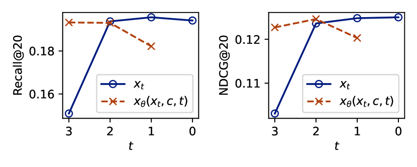
(a) MovieLens-1M.

(b) Yelp.

Figure 5: Performance of reconstructions at different reverse step $t$.

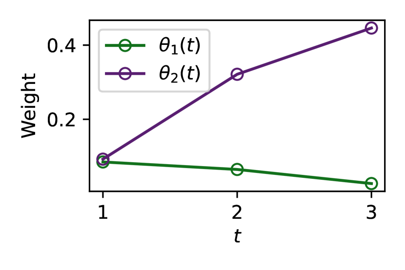
(a) MovieLens-1M.

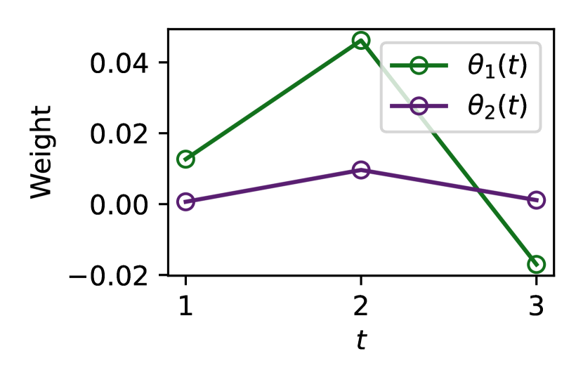
(b) Yelp.

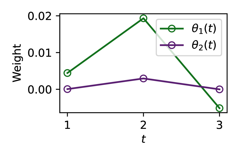
(c) Amazon-Book.

Figure 6: Weighting mechanism at different reverse step $t$.

The hierarchical generative model provides us with a trajectory of ${\bm{x}}_{t}$ along with $\hat{{\bm{x}}}_{\theta}({\bm{x}}_{t},{\bm{c}},t)$, and we are interested in how the quality of these intermediate preference scores changes over the reverse timesteps $t=T,\dots,1$. To this end, we evaluate the performance metrics using ${\bm{x}}_{t}$ and $\hat{{\bm{x}}}_{\theta}({\bm{x}}_{t},{\bm{c}},t)$ for top-$K$ recommendation. The results are in Figure 5, from which we can see that as the sampling proceeds, both Recall@20 and NDCG@20 gradually increase, implying that the reverse process iteratively refines the preference score ${\bm{x}}_{t}$.

We further plot the time-dependent weights $\theta_{1}(t),\theta_{2}(t)$ in Equation 16 and find that, on MovieLens-1M, our denoiser pays more attention to ${\bm{x}}_{t}$ at the early sampling steps while focusing on ${\bm{c}}$ at the later steps. On two sparse datasets, however, our denoiser learns to rely more on ${\bm{x}}_{t}$ throughout sampling, perhaps due to the predominant contribution from the forward process. These observations differ from text-to-image DMs which tend to focus on the conditioning text at the early steps and the image distribution at the later steps (Balaji et al., 2023; Feng et al., 2023).

6 Related Works

DMs for recommendation.

As powerful generative models, DMs have recently garnered attention in the field of recommender systems. Walker et al. (2022) and Wang et al. (2023) studied standard Gaussian diffusion for collaborative filtering; Bénédict et al. (2023) studied binomial diffusion for collaborative filtering; Li et al. (2023); Du et al. (2023); Yang et al. (2023) studied DMs for sequential recommendation; Lin et al. (2023) studied discrete DM for reranking; Liu et al. (2023) studied DM for sequence augmentation; Yu et al. (2023) studied DM for multimedia recommendation. Another work, Choi et al. (2023), designed a graph signal processing technique inspired by DM. Our work is the first to incorporate graph signal processing into the theoretical framework of DM for collaborative filtering.

DMs with general corruptions.

Researchers from various domains have been exploring new forms of diffusion. For example, Bansal et al. (2022) explored cold diffusion without noise; Daras et al. (2022) explored score matching with general linear operators; Rissanen et al. (2022) and Hoogeboom and Salimans (2023) explored diffusion probabilistic models with image blurring filters; Austin et al. (2021) explored discrete DM with general transition probabilities; Hoogeboom et al. (2022) explored equivariant diffusion for 3D graphs; etc. We are the first to explore DMs with graph filters for implicit feedback data, contributing to a generalized form of continuous diffusion.

7 Conclusions

In this work, we propose a novel graph-aware diffusion modeling approach for collaborative filtering with implicit feedback, establishing a new diffusion form with graph smoothing filters and validating the model’s effectiveness through experiments. In the future, research efforts could focus on enhancing the denoiser’s architecture to perform better on sparse datasets. Additionally, exploring the integration of other user-specific conditional information, such as multimodal features, could be an avenue for further investigation.

Appendix A Comments on the Baseline Performance

In this paper, we use the datasets provided by Wang et al. [2023]. However, we do not borrow their existing results and evaluate baselines by ourselves since: (1) We observe that the baseline performance reported by Wang et al. [2023] consistently falls below our own experimental results. (2) We argue that their hyperparameter settings are unfair because they use the default network sizes for MF, LightGCN and Mult-VAE, which is relatively small and results in inferior performance. In contrast, they choose a large embedding size of 1000 for DiffRec on Yelp and Amazon-Book. Actually, the embedding size is essential to recommendation performance, especially when the number of items is huge and low-rank factorization of interaction matrix will cause too much information loss. Similar arguments have been made by Fu et al. [2022]. In our experiments, all the hidden layer sizes, embedding sizes and cut-off dimensions of ideal low-pass filters are consistently set to 200, except for DiffRec and L-DiffRec where we directly take the checkpoints provided by the authors.

References

- Hu et al. (2008) Yifan Hu, Yehuda Koren, and Chris Volinsky. Collaborative Filtering for Implicit Feedback Datasets. In 2008 Eighth IEEE International Conference on Data Mining, pages 263–272, Pisa, Italy, December 2008. IEEE. ISBN 978-0-7695-3502-9. doi:10.1109/ICDM.2008.22. URL http://ieeexplore.ieee.org/document/4781121/.
- Wang et al. (2019) Xiang Wang, Xiangnan He, Meng Wang, Fuli Feng, and Tat-Seng Chua. Neural Graph Collaborative Filtering. In Proceedings of the 42nd International ACM SIGIR Conference on Research and Development in Information Retrieval, pages 165–174, July 2019. doi:10.1145/3331184.3331267. URL http://arxiv.org/abs/1905.08108. arXiv:1905.08108 [cs].
- He et al. (2020) Xiangnan He, Kuan Deng, Xiang Wang, Yan Li, Yongdong Zhang, and Meng Wang. LightGCN: Simplifying and Powering Graph Convolution Network for Recommendation, July 2020. URL http://arxiv.org/abs/2002.02126. arXiv:2002.02126 [cs].
- Fan et al. (2022) Wenqi Fan, Xiaorui Liu, Wei Jin, Xiangyu Zhao, Jiliang Tang, and Qing Li. Graph Trend Filtering Networks for Recommendations, April 2022. URL http://arxiv.org/abs/2108.05552. arXiv:2108.05552 [cs].
- Wu et al. (2016) Yao Wu, Christopher DuBois, Alice X. Zheng, and Martin Ester. Collaborative Denoising Auto-Encoders for Top-N Recommender Systems. In Proceedings of the Ninth ACM International Conference on Web Search and Data Mining, pages 153–162, San Francisco California USA, February 2016. ACM. ISBN 978-1-4503-3716-8. doi:10.1145/2835776.2835837. URL https://dl.acm.org/doi/10.1145/2835776.2835837.
- Liang et al. (2018) Dawen Liang, Rahul G. Krishnan, Matthew D. Hoffman, and Tony Jebara. Variational Autoencoders for Collaborative Filtering, February 2018. URL http://arxiv.org/abs/1802.05814. arXiv:1802.05814 [cs, stat].
- Ma et al. (2019) Jianxin Ma, Chang Zhou, Peng Cui, Hongxia Yang, and Wenwu Zhu. Learning Disentangled Representations for Recommendation, October 2019. URL http://arxiv.org/abs/1910.14238. arXiv:1910.14238 [cs, stat].
- Yu et al. (2019) Xianwen Yu, Xiaoning Zhang, Yang Cao, and Min Xia. VAEGAN: A Collaborative Filtering Framework based on Adversarial Variational Autoencoders. In Proceedings of the Twenty-Eighth International Joint Conference on Artificial Intelligence, pages 4206–4212, Macao, China, August 2019. International Joint Conferences on Artificial Intelligence Organization. ISBN 978-0-9992411-4-1. doi:10.24963/ijcai.2019/584. URL https://www.ijcai.org/proceedings/2019/584.
- Wang et al. (2023) Wenjie Wang, Yiyan Xu, Fuli Feng, Xinyu Lin, Xiangnan He, and Tat-Seng Chua. Diffusion Recommender Model, April 2023. URL http://arxiv.org/abs/2304.04971. arXiv:2304.04971 [cs].
- Rombach et al. (2022) Robin Rombach, Andreas Blattmann, Dominik Lorenz, Patrick Esser, and Björn Ommer. High-Resolution Image Synthesis with Latent Diffusion Models, April 2022. URL http://arxiv.org/abs/2112.10752. arXiv:2112.10752 [cs].
- Chung and Ye (2022) Hyungjin Chung and Jong Chul Ye. Score-based diffusion models for accelerated MRI, July 2022. URL http://arxiv.org/abs/2110.05243. arXiv:2110.05243 [cs, eess].
- Tashiro et al. (2021) Yusuke Tashiro, Jiaming Song, Yang Song, and Stefano Ermon. CSDI: Conditional Score-based Diffusion Models for Probabilistic Time Series Imputation, October 2021. URL http://arxiv.org/abs/2107.03502. arXiv:2107.03502 [cs, stat].
- Ho et al. (2020) Jonathan Ho, Ajay Jain, and Pieter Abbeel. Denoising Diffusion Probabilistic Models, December 2020. URL http://arxiv.org/abs/2006.11239. arXiv:2006.11239 [cs, stat].
- Daras et al. (2022) Giannis Daras, Mauricio Delbracio, Hossein Talebi, Alexandros G. Dimakis, and Peyman Milanfar. Soft Diffusion: Score Matching for General Corruptions, October 2022. URL http://arxiv.org/abs/2209.05442. arXiv:2209.05442 [cs].
- Bansal et al. (2022) Arpit Bansal, Eitan Borgnia, Hong-Min Chu, Jie S. Li, Hamid Kazemi, Furong Huang, Micah Goldblum, Jonas Geiping, and Tom Goldstein. Cold Diffusion: Inverting Arbitrary Image Transforms Without Noise, August 2022. URL http://arxiv.org/abs/2208.09392. arXiv:2208.09392 [cs].
- Rusch et al. (2023) T. Konstantin Rusch, Michael M. Bronstein, and Siddhartha Mishra. A Survey on Oversmoothing in Graph Neural Networks, March 2023. URL http://arxiv.org/abs/2303.10993. arXiv:2303.10993 [cs].
- Rissanen et al. (2022) Severi Rissanen, Markus Heinonen, and Arno Solin. Generative Modelling with Inverse Heat Dissipation. September 2022. URL https://openreview.net/forum?id=4PJUBT9f2Ol.
- Hoogeboom and Salimans (2023) Emiel Hoogeboom and Tim Salimans. Blurring Diffusion Models. 2023.
- Chung (1997) Fan R. K. Chung. Spectral Graph Theory. American Mathematical Soc., 1997. ISBN 978-0-8218-8936-7. Google-Books-ID: YUc38_MCuhAC.
- Shen et al. (2021) Yifei Shen, Yongji Wu, Yao Zhang, Caihua Shan, Jun Zhang, Khaled B. Letaief, and Dongsheng Li. How Powerful is Graph Convolution for Recommendation?, August 2021. URL http://arxiv.org/abs/2108.07567. arXiv:2108.07567 [cs, eess].
- Fu et al. (2022) Hao-Ming Fu, Patrick Poirson, Kwot Sin Lee, and Chen Wang. Revisiting Neighborhood-based Link Prediction for Collaborative Filtering. In Companion Proceedings of the Web Conference 2022, pages 1009–1018, April 2022. doi:10.1145/3487553.3524712. URL http://arxiv.org/abs/2203.15789. arXiv:2203.15789 [cs].
- Choi et al. (2023) Jeongwhan Choi, Seoyoung Hong, Noseong Park, and Sung-Bae Cho. Blurring-Sharpening Process Models for Collaborative Filtering, April 2023. URL http://arxiv.org/abs/2211.09324. arXiv:2211.09324 [cs].
- Newman (2001) M. E. J. Newman. Clustering and preferential attachment in growing networks. Physical Review E, 64(2):025102, July 2001. ISSN 1063-651X, 1095-3787. doi:10.1103/PhysRevE.64.025102. URL http://arxiv.org/abs/cond-mat/0104209. arXiv:cond-mat/0104209.
- Baglama and Reichel (2005) James Baglama and Lothar Reichel. Augmented Implicitly Restarted Lanczos Bidiagonalization Methods. SIAM Journal on Scientific Computing, 27(1):19–42, January 2005. ISSN 1064-8275, 1095-7197. doi:10.1137/04060593X. URL http://epubs.siam.org/doi/10.1137/04060593X.
- Musco and Musco (2015) Cameron Musco and Christopher Musco. Randomized Block Krylov Methods for Stronger and Faster Approximate Singular Value Decomposition. In Advances in Neural Information Processing Systems, volume 28. Curran Associates, Inc., 2015. URL https://proceedings.neurips.cc/paper_files/paper/2015/hash/1efa39bcaec6f3900149160693694536-Abstract.html.
- Ronneberger et al. (2015) Olaf Ronneberger, Philipp Fischer, and Thomas Brox. U-Net: Convolutional Networks for Biomedical Image Segmentation, May 2015. URL http://arxiv.org/abs/1505.04597. arXiv:1505.04597 [cs].
- Kingma et al. (2023) Diederik P. Kingma, Tim Salimans, Ben Poole, and Jonathan Ho. Variational Diffusion Models, April 2023. URL http://arxiv.org/abs/2107.00630. arXiv:2107.00630 [cs, stat].
- Song et al. (2022) Jiaming Song, Chenlin Meng, and Stefano Ermon. Denoising Diffusion Implicit Models, October 2022. URL http://arxiv.org/abs/2010.02502. arXiv:2010.02502 [cs].
- Koren et al. (2009) Yehuda Koren, Robert Bell, and Chris Volinsky. Matrix Factorization Techniques for Recommender Systems. Computer, 42(8):30–37, August 2009. ISSN 0018-9162. doi:10.1109/MC.2009.263. URL http://ieeexplore.ieee.org/document/5197422/.
- Rendle et al. (2012) Steffen Rendle, Christoph Freudenthaler, Zeno Gantner, and Lars Schmidt-Thieme. BPR: Bayesian Personalized Ranking from Implicit Feedback, May 2012. URL http://arxiv.org/abs/1205.2618. arXiv:1205.2618 [cs, stat].
- Kingma and Ba (2017) Diederik P. Kingma and Jimmy Ba. Adam: A Method for Stochastic Optimization, January 2017. URL http://arxiv.org/abs/1412.6980. arXiv:1412.6980 [cs].
- Balaji et al. (2023) Yogesh Balaji, Seungjun Nah, Xun Huang, Arash Vahdat, Jiaming Song, Qinsheng Zhang, Karsten Kreis, Miika Aittala, Timo Aila, Samuli Laine, Bryan Catanzaro, Tero Karras, and Ming-Yu Liu. eDiff-I: Text-to-Image Diffusion Models with an Ensemble of Expert Denoisers, March 2023. URL http://arxiv.org/abs/2211.01324. arXiv:2211.01324 [cs].
- Feng et al. (2023) Zhida Feng, Zhenyu Zhang, Xintong Yu, Yewei Fang, Lanxin Li, Xuyi Chen, Yuxiang Lu, Jiaxiang Liu, Weichong Yin, Shikun Feng, Yu Sun, Li Chen, Hao Tian, Hua Wu, and Haifeng Wang. ERNIE-ViLG 2.0: Improving Text-to-Image Diffusion Model with Knowledge-Enhanced Mixture-of-Denoising-Experts, March 2023. URL http://arxiv.org/abs/2210.15257. arXiv:2210.15257 [cs].
- Walker et al. (2022) Joojo Walker, Ting Zhong, Fengli Zhang, Qiang Gao, and Fan Zhou. Recommendation via Collaborative Diffusion Generative Model. In Knowledge Science, Engineering and Management: 15th International Conference, KSEM 2022, Singapore, August 6–8, 2022, Proceedings, Part III, pages 593–605, Berlin, Heidelberg, August 2022. Springer-Verlag. ISBN 978-3-031-10988-1. doi:10.1007/978-3-031-10989-8_47. URL https://doi.org/10.1007/978-3-031-10989-8_47.
- Bénédict et al. (2023) Gabriel Bénédict, Olivier Jeunen, Samuele Papa, Samarth Bhargav, Daan Odijk, and Maarten de Rijke. RecFusion: A Binomial Diffusion Process for 1D Data for Recommendation, September 2023. URL http://arxiv.org/abs/2306.08947. arXiv:2306.08947 [cs].
- Li et al. (2023) Zihao Li, Aixin Sun, and Chenliang Li. DiffuRec: A Diffusion Model for Sequential Recommendation, April 2023. URL http://arxiv.org/abs/2304.00686. arXiv:2304.00686 [cs].
- Du et al. (2023) Hanwen Du, Huanhuan Yuan, Zhen Huang, Pengpeng Zhao, and Xiaofang Zhou. Sequential Recommendation with Diffusion Models, June 2023. URL http://arxiv.org/abs/2304.04541. arXiv:2304.04541 [cs].
- Yang et al. (2023) Zhengyi Yang, Jiancan Wu, Zhicai Wang, Xiang Wang, Yancheng Yuan, and Xiangnan He. Generate What You Prefer: Reshaping Sequential Recommendation via Guided Diffusion, October 2023. URL http://arxiv.org/abs/2310.20453. arXiv:2310.20453 [cs].
- Lin et al. (2023) Xiao Lin, Xiaokai Chen, Chenyang Wang, Hantao Shu, Linfeng Song, Biao Li, and Peng jiang. Discrete Conditional Diffusion for Reranking in Recommendation, August 2023. URL http://arxiv.org/abs/2308.06982. arXiv:2308.06982 [cs].
- Liu et al. (2023) Qidong Liu, Fan Yan, Xiangyu Zhao, Zhaocheng Du, Huifeng Guo, Ruiming Tang, and Feng Tian. Diffusion Augmentation for Sequential Recommendation, September 2023. URL http://arxiv.org/abs/2309.12858. arXiv:2309.12858 [cs].
- Yu et al. (2023) Penghang Yu, Zhiyi Tan, Guanming Lu, and Bing-Kun Bao. LD4MRec: Simplifying and Powering Diffusion Model for Multimedia Recommendation, September 2023. URL http://arxiv.org/abs/2309.15363. arXiv:2309.15363 [cs].
- Austin et al. (2021) Jacob Austin, Daniel D. Johnson, Jonathan Ho, Daniel Tarlow, and Rianne van den Berg. Structured Denoising Diffusion Models in Discrete State-Spaces. In Advances in Neural Information Processing Systems, volume 34, pages 17981–17993. Curran Associates, Inc., 2021. URL https://proceedings.neurips.cc/paper_files/paper/2021/hash/958c530554f78bcd8e97125b70e6973d-Abstract.html.
- Hoogeboom et al. (2022) Emiel Hoogeboom, Vıictor Garcia Satorras, Clement Vignac, and Max Welling. Equivariant Diffusion for Molecule Generation in 3D. In Proceedings of the 39th International Conference on Machine Learning, pages 8867–8887. PMLR, June 2022. URL https://proceedings.mlr.press/v162/hoogeboom22a.html. ISSN: 2640-3498.