High-Resolution Particle-In-Cell Simulations of Two-Dimensional Bernstein-Greene-Kruskal Modes

Abstract

We present two dimensional (2D) particle-in-cell (PIC) simulations of 2D Bernstein-Greene-Kruskal (BGK) modes, which are exact nonlinear steady-state solutions of the Vlasov-Poisson equations, on a 2D plane perpendicular to a background magnetic field, with a cylindrically symmetric electric potential localized on the plane. PIC simulations are initialized using analytic electron distributions and electric potentials from the theory. We confirm the validity of such solutions using high-resolutions up to a $2048^{2}$ grid. We show that the solutions are dynamically stable for a stronger background magnetic field, while keeping other parameters of the model fixed, but become unstable when the field strength is weaker than a certain value. When a mode becomes unstable, we observe that the instability begins with the excitation of azimuthal electrostatic waves that ends with a spiral pattern.

I INTRODUCTION

One remarkable property of high-temperature collisionless plasmas is the possibility of forming small-scale kinetic structures known as Bernstein-Greene-Kruskal (BGK) modes, Bernstein, Greene, and Kruskal (1957) which can be theoretically described as exact nonlinear steady-state solutions that satisfy the Vlasov and Poisson equations self-consistently. The original BGK mode solutions are in one dimension (1D), with the solution being invariant along one Cartesian coordinate. Analytic solutions of BGK modes were later generalized to 3D for an unmagnetized plasma, Ng and Bhattacharjee (2005) with a spherically symmetric electric potential localized in all spatial directions; as well as 2D, for a magnetized plasma in a uniform background magnetic field, Ng, Bhattacharjee, and Skiff (2006); Ng (2020) with a cylindrically symmetric potential localized on a 2D plane perpendicular the background field. Much more research has been done on the subject of BGK modes. Please refer to a recent paper, Ref. Ng, 2020, for a more complete discussion on physical motivations and relevant literature along this line of research.

Preliminary low-resolution 2D particle-in-cell (PIC) simulations of 2D BGK modes Ng, Bhattacharjee, and Skiff (2006); Ng (2020) have been reported before, Ng, Soundararajan, and Yasin (2012) showing a qualitative trend that the modes are more stable in the limit of strong background magnetic field strength, and unstable in the opposite limit. In this paper, we report 2D PIC simulations of such 2D BGK modes in much higher resolutions (using grids of cells up to $2048^{2}$), using the Plasma Simulation Code (PSC), Germaschewski et al. (2016) a fully electromagnetic PIC code, running in parallel on supercomputers.

The main objectives of this research are to confirm the validity of analytic solutions, Ng, Bhattacharjee, and Skiff (2006); Ng (2020) quantify how the stability of such modes depends on key parameters such as the background magnetic field strength, and to observe the dynamical evolutions of the modes after they become unstable. In section II, we briefly summarize the theory of the 2D BGK modes. Ng, Bhattacharjee, and Skiff (2006); Ng (2020) In section III, we describe the numerical setup of the PIC simulations. Main results from these simulations are presented in section IV. Based on these results, we discuss and conclude in section V on how the above objectives are met. In short, our results will show that the analytic solutions of the 2D BGK modes are indeed valid for the Vlasov-Poisson equations, and that such solutions are stable in 2D for our choice of parameters with the normalized strength of the background magnetic field $B_{0}\gtrsim 2$ (defined in the next section) for our choice of other parameters, while azimuthal electrostatic waves are excited when a mode becomes unstable.

II BGK MODE SOLUTIONS

II.1 Theory

The Vlasov equation is the continuity equation for a distribution function $f$ over position $(x_{1},x_{2},x_{3})$ and velocity $(v_{1},v_{2},v_{3})$ space,

$$\frac{\partial f}{\partial t}+\sum_{i=1}^{3}\frac{\partial f}{\partial x_{i}}\frac{\text{d}x_{i}}{\text{d}t}+\sum_{i=1}^{3}\frac{\partial f}{\partial v_{i}}\frac{\text{d}v_{i}}{\text{d}t}=0.$$ (1)

We consider the case with a uniform ion density $n_{i}$ and a uniform background magnetic field $\vv{B}_{0}=B_{0}\hat{z}$. In cylindrical coordinates, $(x_{1},x_{2},x_{3};v_{1},v_{2},v_{3})=(\rho,\phi,z;v_{\rho},v_{\phi},v_{z})$.

We normalize according to

$$e\equiv q_{i}=-q_{e} \to 1$$ (2a)

$$m_{e} \to 1$$ (2b)

$$n_{i}=n_{e}\rvert_{\rho=\infty} \to 1$$ (2c)

$$\epsilon_{0} \to 1$$ (2d)

$$\omega_{\text{pe}}\equiv\sqrt{\frac{e^{2}n_{e}}{\epsilon_{0}m_{e}}} \to 1$$ (2e)

$$v_{e}\equiv\sqrt{\frac{k_{B}T_{e}}{m_{e}}} \to 1.$$ (2f)

The normalizations (2e) and (2f) imply that the Debye length $\lambda_{\text{D}}\equiv v_{e}/\omega_{\text{pe}}=1$. The electric potential $\psi$ has units $m_{e}v_{e}^{2}/e$, and the magnetic field strength $B_{0}$ has units $em_{e}/n_{e}\omega_{\text{pe}}$. Note that $B_{0}=\omega_{\text{c}}/\omega_{\text{pe}}$, where $\omega_{\text{c}}\equiv eB/m_{e}$ is the electron gyrofrequency. Thus, the electron gyroperiod $\tau_{c}\equiv 2\pi/\omega_{\text{c}}$ is $2\pi/B_{0}$.

Imposing spatial symmetries $\frac{\partial}{\partial\phi}=\frac{\partial}{\partial z}=0$ and the steady-state condition $\frac{\partial}{\partial t}=0$ on the Vlasov-Poisson equations obtains

$$\begin{split}\frac{\partial f}{\partial\rho}v_{\rho}+\frac{\partial f}{\partial v_{\rho}}\left(\frac{\partial\psi}{\partial\rho}-B_{0}v_{\phi}+\frac{v_{\phi}^{2}}{\rho}\right)+&\\ \frac{\partial f}{\partial v_{\phi}}\left(B_{0}v_{\rho}-\frac{v_{\rho}v_{\phi}}{\rho}\right)&=0,\end{split}$$ (3)

$$\frac{1}{\rho}\frac{\partial}{\partial\rho}\left(\rho\frac{\partial\psi}{\partial\rho}\right)=\int\text{d}^{3}vf-1.$$ (4)

When $f$ depends only on energy $w=\frac{1}{2}v^{2}-\psi$, it cannot satisfy (4) and remain localized. Ng (2020) Including a dependence on the canonical angular momentum $l=\rho v_{\phi}-\frac{1}{2}B_{0}\rho^{2}$ makes a localized solution possible. One possible form is

$$f(w,l)=(2\pi)^{-3/2}e^{-w}\left(1-he^{-kl^{2}}\right)$$ (5)

where $h\in(-\infty,1)$ and $k\in(0,\infty)$ are constant parameters. The potential $\psi=\psi(\rho)$ must be solved numerically using Eq. (4), with $f$ given by Eq. (5),

$$\frac{1}{\rho}\frac{\partial}{\partial\rho}\left(\rho\frac{\partial\psi}{\partial\rho}\right)=e^{\psi}\left[1-\frac{h}{\gamma}\exp\left(-\frac{kB_{0}^{2}\rho^{4}}{4\gamma^{2}}\right)\right]-1$$ (6)

where

$$\gamma\equiv\gamma(\rho) \mathrel{\coloneqq}\sqrt{1+2k\rho^{2}}$$ (7)

The resulting configuration can be described as follows. Starting with a uniform distribution, electrons near the origin have been scooped out and deposited in a ring around the origin. This leads to an outward $E_{\rho}$. Additionally, the electrons in the ring have been given a slight clockwise flow. The configuration can therefore be described as an electron vortex circulating around an electron density hole. Figures 2 and 8 illustrate electron distributions for different values of $B_{0}$ at time $t=0$ and later.

II.2 Approximations

These solutions assume a static magnetic field $\vv{B}=B_{0}\hat{x}$. Induced magnetic fields due to plasma current were negligible even for $B_{0}=0.1$, the lowest value of $B_{0}$ considered in this paper. This is due to our choice of the parameter $\beta_{e}=v_{e}/c=0.001$.

Although the plasma in these simulations is very cold, with $k_{B}T=0.511$ eV, and is magnetically dominated with a plasma beta of $2\times 10^{-6}$ when $B_{0}=1$, the solution given by Eqs. (5) and (6) does not depend on $\beta_{e}$ explicitly. Therefore, they are valid if a larger $\beta_{e}$ value is used, as long as the physics remains in the non-relativistic regime. The small $\beta_{e}$ value used in the relativistic PSC simulations is to make sure the outputs can be compared with the non-relativistic theory. For larger $\beta_{e}$, Ampère’s Law would need to be solved alongside Eq. (6) to obtain a self-consistent magnetic field. Ng (2020) For the relativistic case with $\beta_{e}\rightarrow 1$, the relativistic Vlasov equation would need to be employed instead. These generalizations are left for future studies, and will not be considered in this paper.

An ostensibly less justifiable approximation was that ions formed a uniform static background. It is possible to ease this restriction and find theoretical solutions with realistic proton behavior,Tang (2020) and several runs of this nature were performed. However, such runs were found to be qualitatively similar to motionless-ion runs, and we will not be exploring them further in this paper.

III NUMERICAL SETUP

III.1 Normalization

PSC and figures shown below are normalized according to Eq. (2) with the change

$$c \to 1.$$ (8)

Thus, time still has units of $\omega_{\text{pe}}^{-1}$, but distance now has units of the electron skin depth, $c\omega_{\text{pe}}^{-1}$. This multiplies the length scale compared to Eq. (2) by a factor of $\beta_{e}=v_{e}/c=0.001$.

III.2 Parameters

All runs used constants $h=0.9$, $k=0.4$ (see Eq. (5)) and electron thermal velocity $v_{e}=c/1000$. Equation (6) was solved numerically in an external program to obtain $\psi(\rho)$. Ions had unit charge and masses of $10^{9}$ to mimic a static, uniform background of normalized density $n_{i}=1$.

The physical domain for each run was square centered at the origin. Boundaries were periodic. The side length of the domain was automatically fine-tuned for each value of $B_{0}$ to be large enough to avoid strong edge effects, but no larger, since resolving the central hole became difficult for $B_{0}\lesssim 1$. The lengths are given in Table 1.

Table 1: Side lengths of the square domain used in simulations for different values of $B_{0}$.

$B_{0}$	length
0.1	0.180062
0.25	0.072156
0.5	0.036307
1	0.020960
2	0.017530
4	0.015464
10	0.013264

III.3 Field and Density Initialization

Since $\psi(\rho)$ was solved externally, its discretized form had to be transferred to PSC by file. Support for input-by-file was implemented in PSC for this purpose. PSC then interpolates $\psi(\rho)$ onto its grid and computes the first-order discrete gradient to find the electric field.

Electron number density $n_{e}$ is computed as $n_{i}=1$ minus the first-order discrete divergence of $\vv{E}$. For both electrons and ions, a number density of 1 corresponds to 100 macroparticles per cell (nicell=100) unless otherwise specified. This means that higher-resolution runs generally had more macroparticles.

The magnetic field was simply initialized to $\vv{B}(t=0)=B_{0}\hat{x}$ at every grid point.

III.4 Velocity Initialization

A major limitation of PSC was that it used the Box-Muller method to sample velocities during particle initialization. This method is efficient but produces a normal distribution with a given mean and variance. The radial component of velocity is indeed normally distributed according to (5), but the azimuthal component $v_{\phi}$ is not, as shown in Fig. 1. Note that the unit of velocity is the speed of light $c$ in this figure, and other figures of this paper, following the default unit used in PSC.

Early runs, called “moment” runs, simply approximated the true distribution as a local Maxwellian with the same density, mean velocity, and temperature. We later extended PSC to support arbitrary initial distribution functions using an inverse-CDF method. Runs initialized using this method are called “exact” runs.

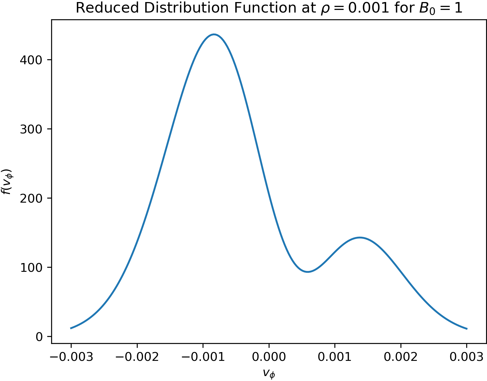
Figure 1: Reduced electron distribution function $f(v_{\phi})$ at a point one Debye length from the origin for the $B_{0}=1$ case. All cases feature non-Maxwellian azimuthal velocity distributions, but local minima appear for $B_{0}\lesssim 2$, with other parameters fixed.

IV NUMERICAL RESULTS

Four categories of runs were performed: moment, moment reversed, exact, and exact reversed. “Reversed” cases, intended to serve as non-examples to contrast with the steady-state cases, were initialized exactly the same as non-reversed cases except that $v_{\phi}$ was negated. Many runs were performed within each category, varying $B_{0}$ from $0.1$ to $10$ and on grids of size $256^{2}$, $512^{2}$, and for some cases up to $2048^{2}$.

Note that in the figures of this paper, we use the electron skin depth $c/\omega_{pe}$ as the unit of spatial length, which is the default unit used in PSC, and corresponds to $10^{3}$ Debye lengths for our choice of $v_{e}$ as discussed in section III.1. From Fig. 2 we see that the electron density holes have a size on the order of $\lambda_{D}$. Also following the convention of PSC, the background magnetic field is along the $x$-direction, so the 2D simulation plane is the $y$-$z$ plane.

IV.1 Moment Runs

Due to technical limitations of PSC (as discussed in section III.4), early runs used a moment-based approximation of the electron velocity distribution. For $B_{0}\gtrsim 4$, runs were more or less steady-state, remaining stable for the duration of the simulations. Moment runs with $B_{0}\lesssim 2$, however, were not steady-state. Pulsation was observed for many cases, and are more obvious for $0.5\lesssim B_{0}\lesssim 2$. Runs with $B_{0}\lesssim 0.25$ completely decayed in a short period of time. Fig. 2 shows snapshots of low-, mid-, and high-$B_{0}$ moment runs demonstrating these phenomena.

In contrast to normal moment runs with high $B_{0}$, moment reversed runs with high $B_{0}$ pulsated strongly. No moment reversed run was steady-state, as expected. For each $B_{0}$, the reversed run breathed more strongly than the non-reversed run (except for $B_{0}=0.1$, which decayed quickly in both cases).

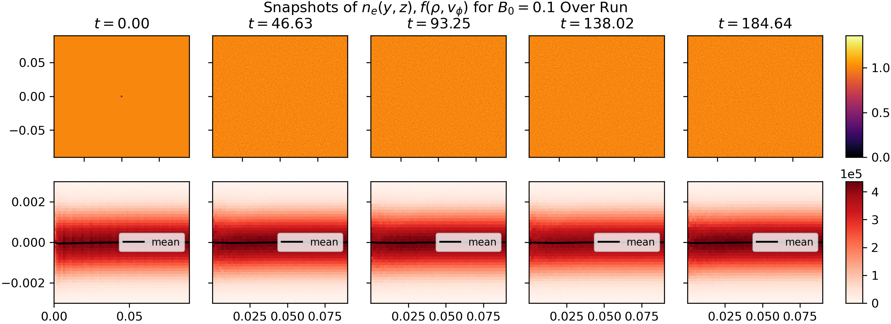
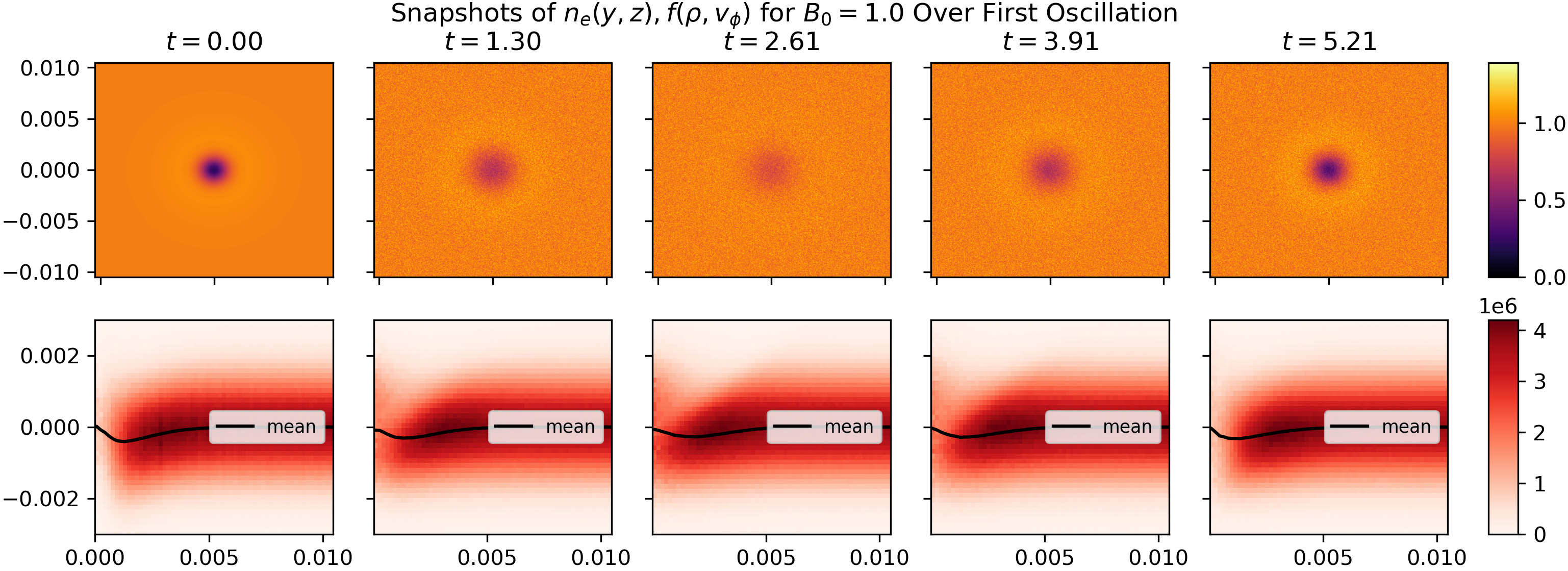
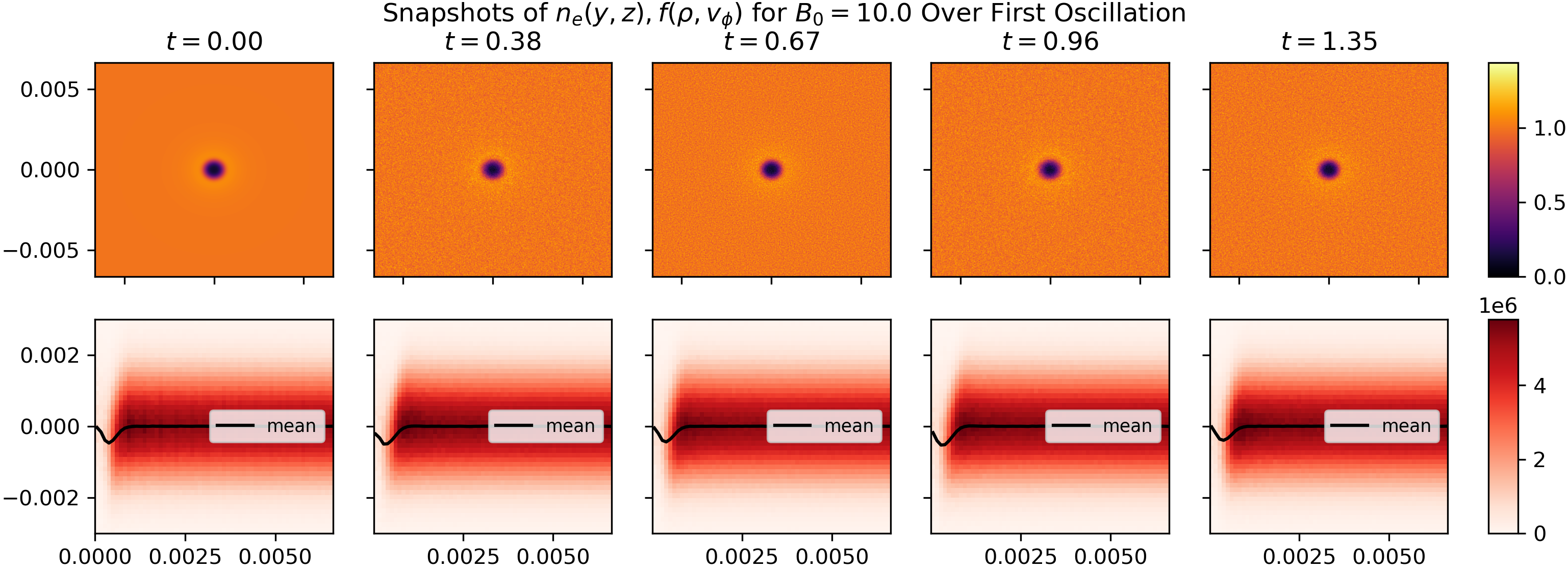
Figure 2: Sequences of $f(y,z)$ and $f(\rho,v_{\phi})$ for moment runs over one oscillation for $B_{0}\geq 1$, or over the whole run for $B_{0}=0.1$ which did not oscillate. Note the pulsation for $B_{0}=1$ involves a collapse of the hole and formation of a “spike” in velocity space, discussed in section IV.1.4.

IV.1.1 Nearly Stable: $B_{0}=4$, Moment

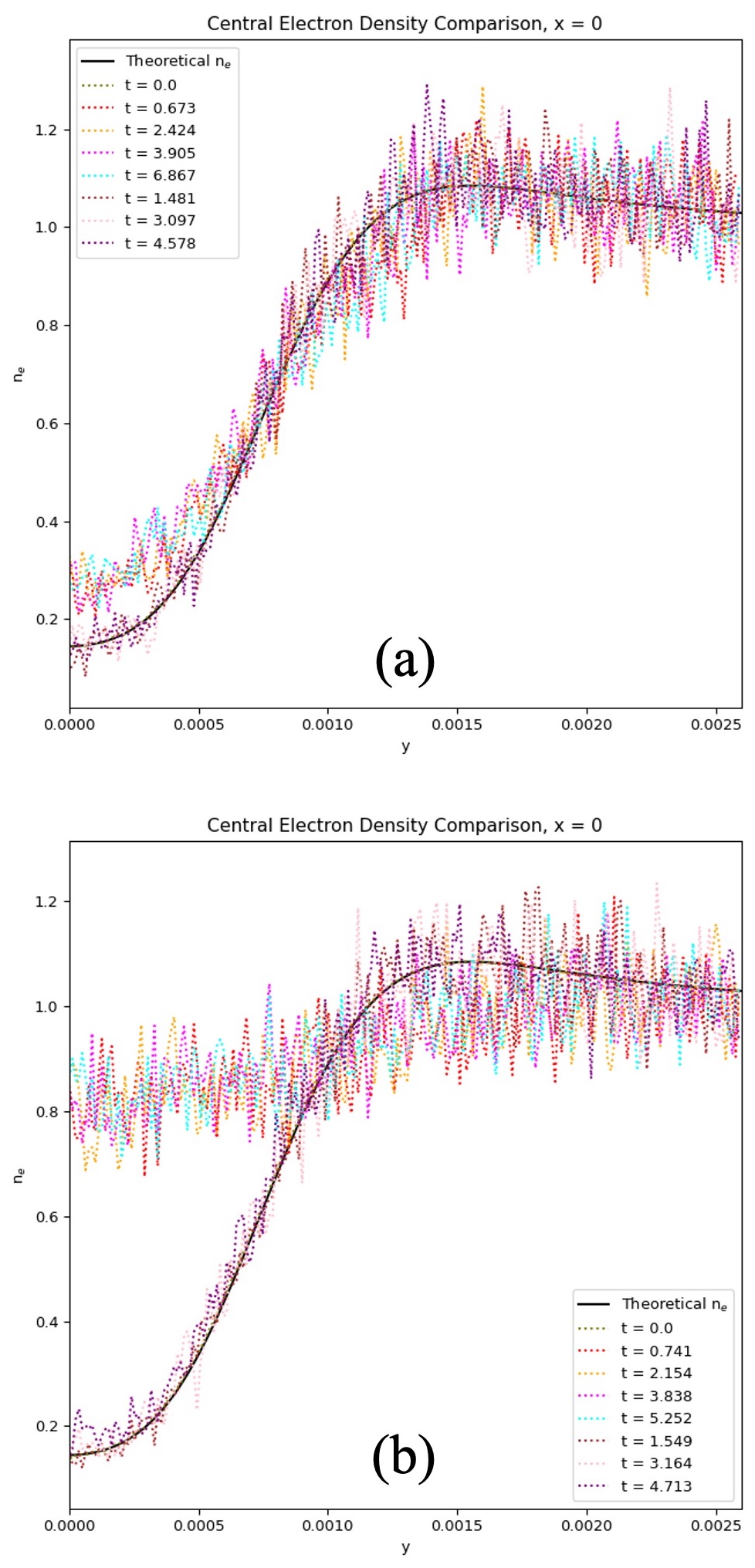
Figure 3: Electron density $n_{e}$ along the $y$-axis at indicated times from two PIC simulations with $B_{0}=4$ using a $2048^{2}$ grid, for (a) the normal-flow moment case, and (b) the reserved-flow moment case. The black continuous curves on both panels are the input $n_{e}$ profiles for the analytic BGK mode.

We now look at a specific case with $B_{0}=4$ to compare the moment runs with normal and reversed flow in more details. Fig. 3 shows curves of $n_{e}$ vs $y$ along the $y$-axis at different instants within about three $\tau_{c}=2\pi/\omega_{\text{c}}=\pi/2$, for the normal case in panel (a) and the reversed case in panel (b). These instants are chosen when the $n_{e}$ value at the origin are roughly the largest or smallest during one $\tau_{c}$. Therefore, $n_{e}$ curves between two instants are somewhere in between the corresponding two groups of curves that are shown. The black continuous curves on both panels are the input $n_{e}$ profiles for the analytic BGK mode.

PIC simulations are known to suffer from noise due to finite particle number. 10.1063/1.862452 The curves in Fig. 3 demonstrate this, despite being from runs with our largest grid size of $2048^{2}$ cells. The noise is low enough that the pulsation amplitude for both normal and reversed case is resolved. While the noise level is about the same for the normal and reversed cases, the reversed case has a much larger pulsation amplitude. Based on this result and similar results for every other relevant case, we conclude that the difference in behavior is based on true dynamics, not numerical noise.

The fact that the normal flow case has a small pulsation amplitude, as compared with the reversed flow case, as well as the initial depletion of $n_{e}$ at the center, shows that the BGK-like initial condition does represent a more time-steady and stable case. By BGK-like, we mean this configuration only matches the three lowest-order moments (density, flow velocity, and effective temperature) of the true BGK mode solution. Such a configuration cannot represent the non-Maxwellian distribution as shown in Fig. 1, especially for low $B_{0}$. Nevertheless, the above results do show that even just matching the moments can make a configuration approximately time-steady in the strong $B_{0}$ limit.

We have put many simulation movies into the Supplemental Materials, including the two density movies corresponding to Fig. 3. The movies for these two runs provide a better contrast between the different pulsation levels for the two cases.

IV.1.2 General Trends

Generally, the pulsation level is larger for smaller $B_{0}$, and much larger for the reversed case than the normal case. The $n_{e}$ value at the center can be greater than unity at times for smaller $B_{0}$ cases. This value as a function of time turns out to be a simple visualization to show the pulsation of a run. Figs. 4, 5, and 6 show the spatial averaged $n_{e}$ value at the center, $n_{e0}$, as functions of time, for $B_{0}$ in the weak, medium, and strong ranges (with overlaps).

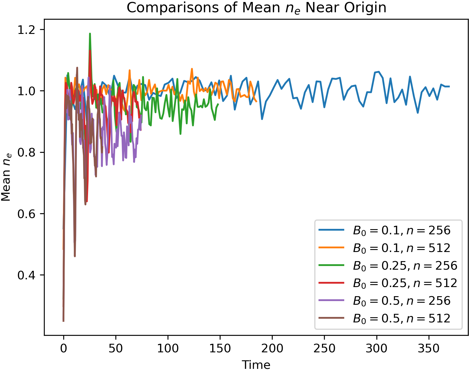
Figure 4: Electron density $n_{e}$ at the center for $B_{0}=0.1$, 0.25, and $0.5$ using $256^{2}$ and $512^{2}$ grids for moment runs.

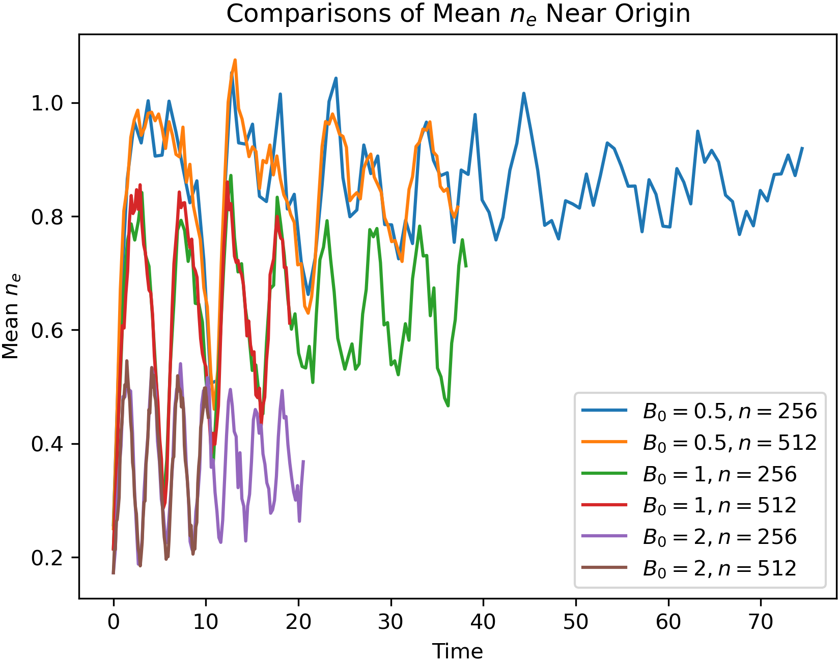
Figure 5: Electron density $n_{e}$ at the center for $B_{0}=0.5$, 1, and 2 using $256^{2}$ and $512^{2}$ grids for moment runs.

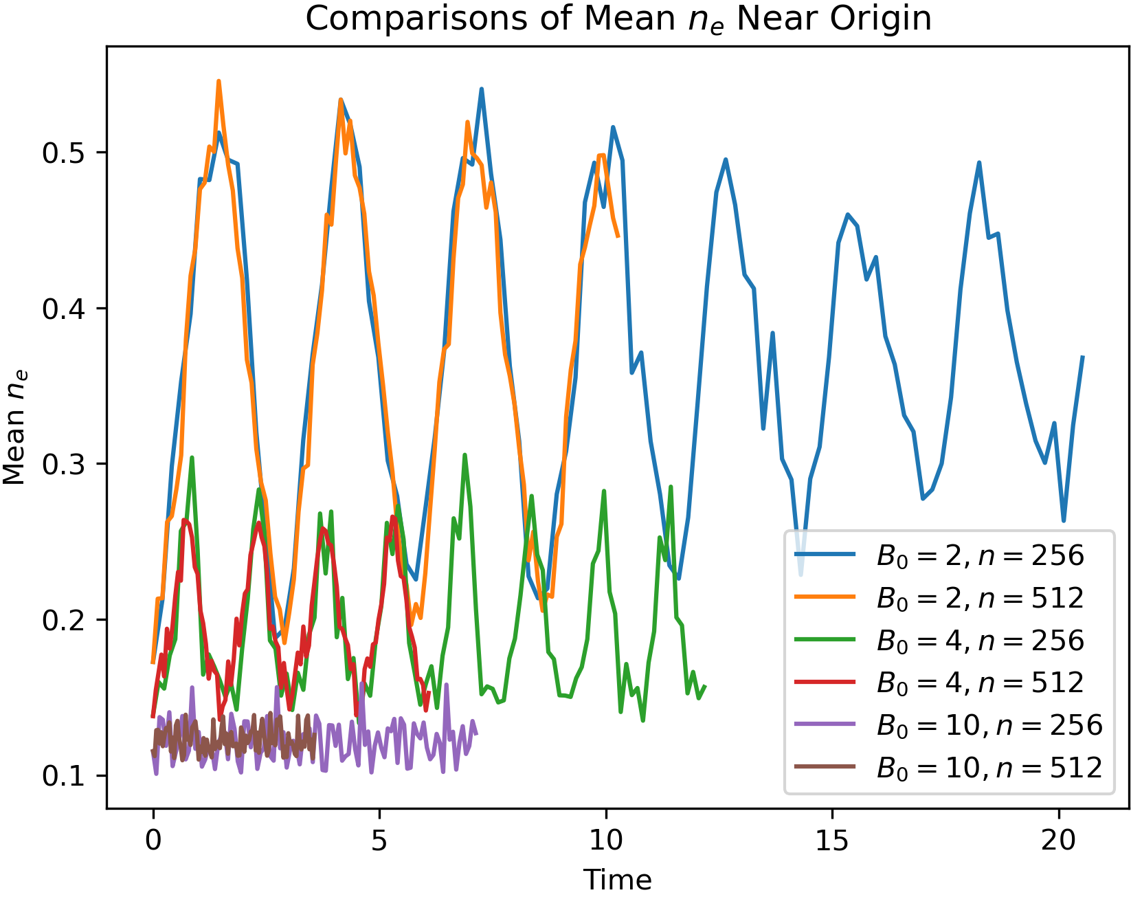
Figure 6: Electron density $n_{e}$ at the center for $B_{0}=2$, 4, and 10 using $256^{2}$ and $512^{2}$ grids for moment runs.

In Figures 4, 5 and 6, we show two sets of curves using $256^{2}$ and $512^{2}$ grids to show the possible dependence on resolution. The figures indicate that the plasma behavior is essentially the same for the two grid resolutions. Therefore, the dynamics of the moment runs are adequately resolved using a resolution of $256^{2}$ or higher.

IV.1.3 Pulsation Frequency

Angular frequencies of the pulsating behavior of moment runs are given in Table 2. These values were obtained by taking a Fourier transform of the mean electron density in the middle 4 cells of the $256^{2}$ runs, or an equivalent-sized square area for higher-resolution runs. The angular frequency $\Omega$ is then $2\pi$ times the frequency with the largest amplitude. Although minor, pulsation for high-$B_{0}$ moment runs were detectable using this method.

Table 2: Angular oscillation frequencies $\Omega$ of moment and moment reversed runs on $256^{2}$ grids, or $512^{2}$ grids for $B_{0}<1$.

$B_{0}$	$\Omega$	$\Omega_{\text{rev}}$
0.1	—	—
0.25	0.320	0.232
0.5	0.635	0.509
1	1.24	1.06
2	2.27	2.14
4	4.21	4.16
10	10.2	10.2

The angular frequencies are very close to the electron gyrofrequency $\omega_{ce}$, especially for reversed runs and for runs with higher $B_{0}$. The discrepancy can in part be explained by the effects of the electron $E\times B$ drift in a cylindrically symmetric radial electric field, which increase the effective gyrofrequency for non-reversed cases more than the reversed cases, since the electric field magnitude oscillates (even with sign reversal) for the latter. This hints that the pulsation is due to gyromotion.

Another look at the velocity-space distributions in Fig. 2 suggests that electrons gyrate between the “spike” region and the central hole. The spike region is present in Eq. (5), as Fig. 7 shows and of which Fig. 1 is a vertical, renormalized cross section. Indeed, the spike region seems to lie on the line where an electron’s gyrodiameter $2\lvert v_{\phi}\rvert/B_{0}$ equals its radial coordinate $\rho$ and gyromotion would take an electron at $\rho$ inward to near the origin, and an electron near the origin outward to this $\rho$ location. This analysis led in part to support in PSC for initialization of the true electron distribution function, as described in section III.4.

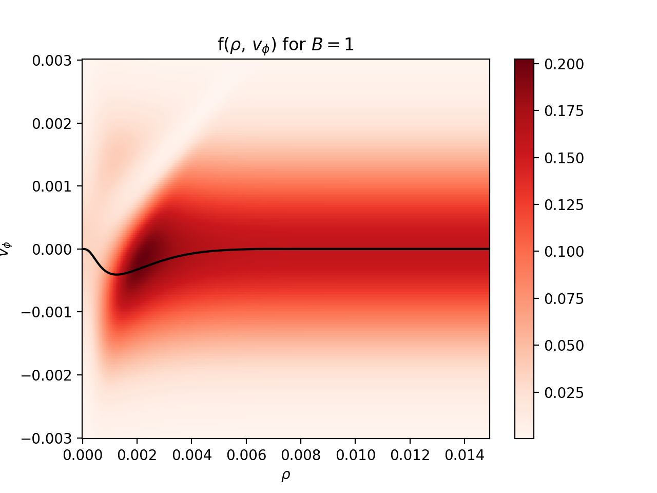
Figure 7: The reduced electron distribution $f(\rho,v_{\phi})$ has a depleted “spike” region extending through the $(\rho,v_{\phi})$ space. The spike is steeper for higher $B_{0}$, disappearing into the hole itself.

IV.1.4 Spike Region

Rewriting Eq. (5) in terms of $\rho,v_{\rho},$ and $v_{\phi}$ reveals it to be the difference of two Gaussians (note the normalization is by Eq. (2), not Eq. (8)):

$$\frac{\int\text{d}v_{\rho}\text{d}v_{z}f}{\int\text{d}^{3}vf}=\frac{1}{\alpha}\frac{1}{\sqrt{2\pi}}e^{-\frac{1}{2}v_{\phi}^{2}}\\ +\left(1-\frac{1}{\alpha}\right)\frac{\gamma}{\sqrt{2\pi}}e^{-\frac{1}{2}\gamma^{2}\left(v_{\phi}-{kB_{0}\rho^{3}}/{\gamma^{2}}\right)^{2}}$$ (9)

where

$$\alpha\equiv\alpha(\rho) \mathrel{\coloneqq}1-\frac{h}{\gamma}e^{-{kB_{0}^{2}\rho^{4}}/{4\gamma^{2}}}.$$ (10)

The spike is caused by the shifted Gaussian having a negative coefficient, i.e., $1-1/\alpha<0$. The negative Gaussian is centered at $v_{\phi}=kB_{0}\rho^{3}/\gamma^{2}$, which for $\rho>1$ (or in PSC units: $\rho>.001$) gives $v_{\phi}\approx\frac{1}{2}B_{0}\rho$. Ignoring the effect of $v_{\rho}$, which is normally distributed with a mean of 0, this is the condition for an electron to have a gyrodiameter equal to its distance from the origin and to gyrate towards the origin.

The spike itself is not centered at the negative Gaussian, but slightly higher, due to the influence of the positive Gaussian. This shift is such that not only does $v_{\phi}\to\frac{1}{2}B_{0}\rho$, but $\rho v_{\phi}\to\frac{1}{2}B_{0}\rho^{2}$, i.e., $l\to 0$. Note that the mean of the negative Gaussian does not satisfy the latter condition.

IV.2 Exact Runs

Exact runs, initialized according to the true electron distribution function, did not pulsate like the moment runs. Figure 8 gives snapshots of low-, mid-, and high-$B_{0}$ exact runs. Note the spike regions are present at $t=0$, and both the density hole and velocity-space spike persists somewhat even for low-$B_{0}$ cases.

Periodicity was not detectable using the FFT method described in LABEL:sec:pulsationfrequency. Videos do seem to exhibit periodicity, however: macroparticles return to their initial configuration at the end of every gyroperiod, briefly returning the system to a relatively smooth state in between noisy periods.

Exact reversed runs behaved similarly to moment reversed runs and do not merit further discussion.

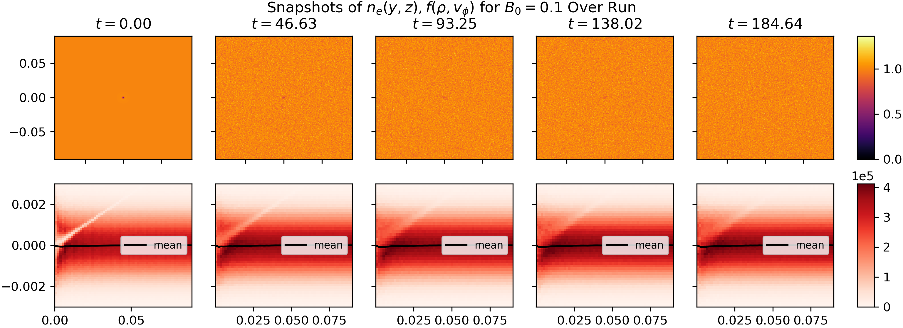
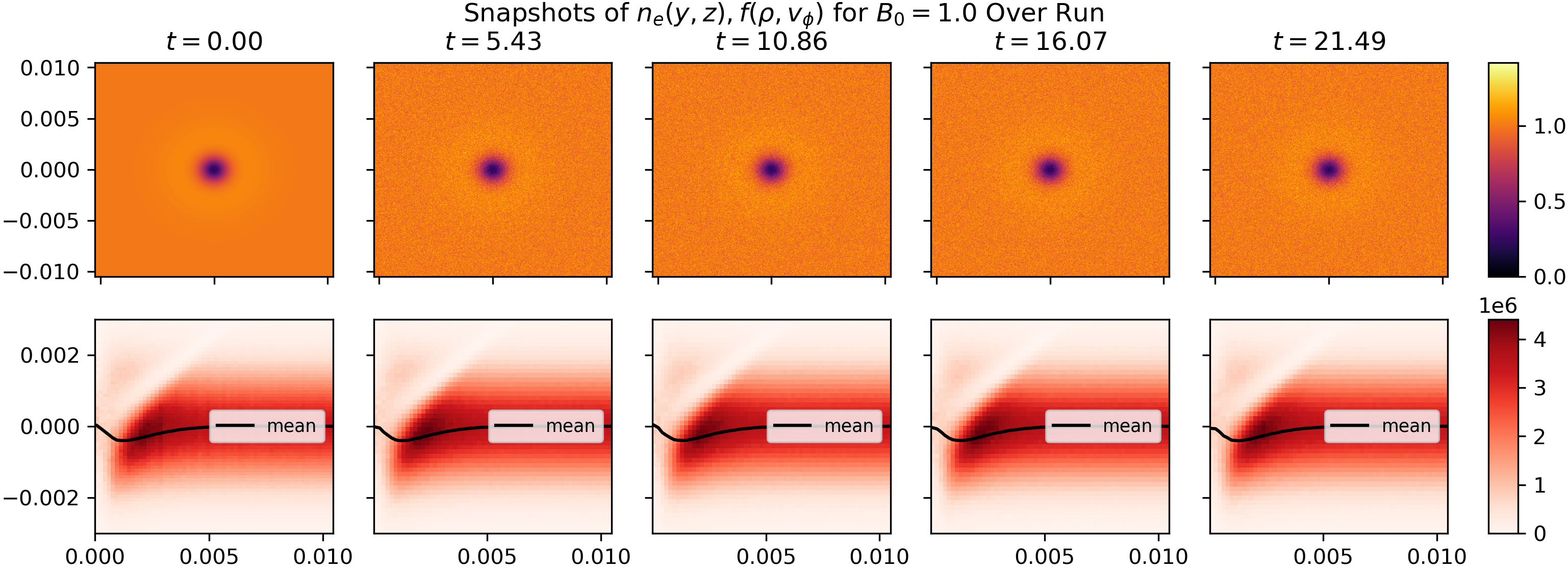
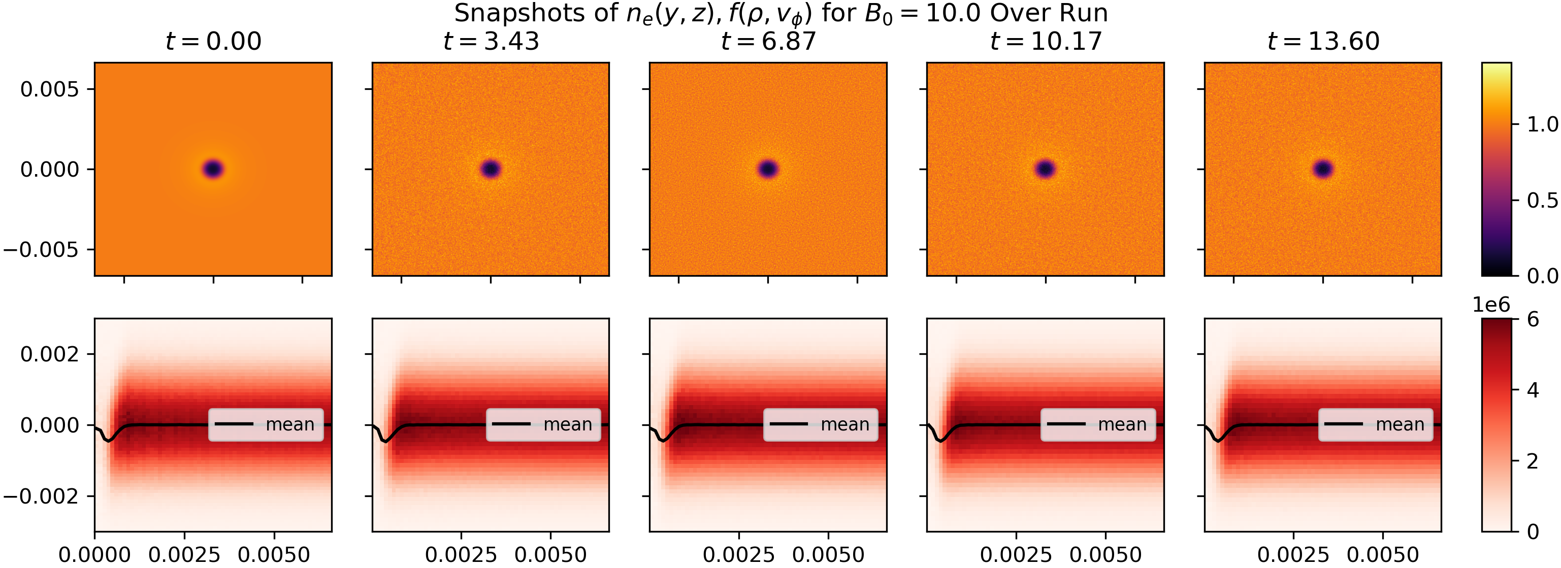
Figure 8: Sequences of $f(y,z)$ and $f(\rho,v_{\phi})$ for “exact” runs.

IV.2.1 Truly Stable: $B_{0}=4$, Exact

With the pulsating behavior gone, we were able to determine whether the analytic form was time-steady or not, and if so, whether it was stable or unstable. We use $B_{0}=4$ as an example again to contrast it with the results discussed in section IV.1.1, and because the magnetic field was strong enough that the configuration was stable.

Figure 9 shows plots using data from four runs with $B_{0}=4$. In addition to the moment and moment reversed runs using $2048^{2}$ grids from Fig. 3, we show a $2048^{2}$ run initialized exactly. Its total duration is again not very long—up to $t\sim 6.3$, or about 4 $\tau_{c}$—since it is computationally expensive to run at such a high resolution. To see the long term behavior, we performed another exact $B_{0}=4$ run using a $256^{2}$ grid and ran it up to $t\sim 320\sim 204\tau_{c}$.

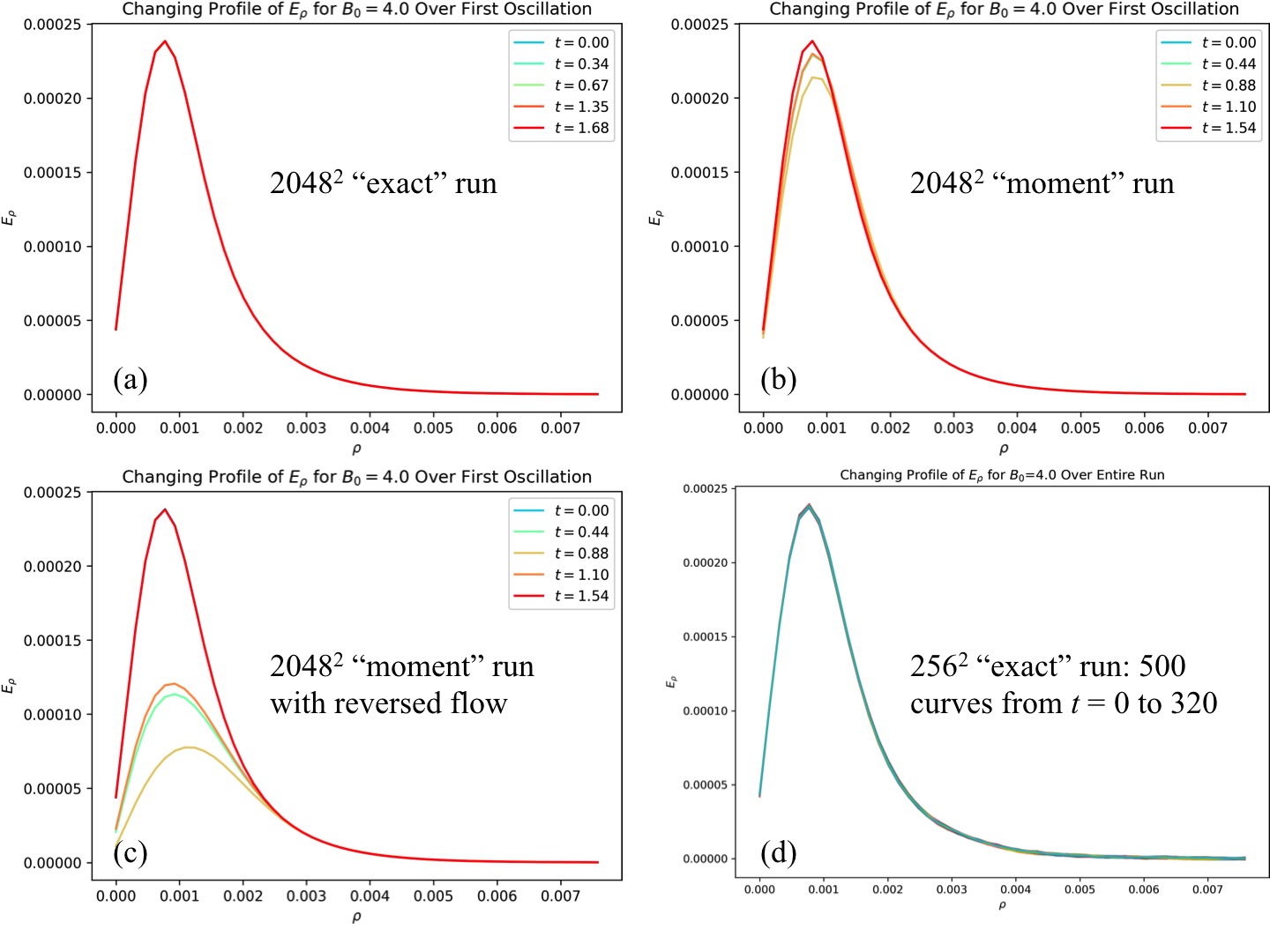
Figure 9: Profiles of the radial electric field component $E_{\rho}$, averaged over all azimuthal angles, as functions of $\rho$, for (a) an exact $2048^{2}$ run, (b) a moment $2048^{2}$ run, (c) a moment reversed $2048^{2}$ run, and (d) an exact $256^{2}$ run. Five curves each are plotted in the first three panels, over about one $\tau_{c}$. 500 curves are plotted in (d), equally spaced over the entire duration of the run.

To show the time-steadiness of the exact runs, we plot the radial electric field component $E_{\rho}$, averaged over all azimuthal angles, as a function of $\rho$, the radial position. This averaging removes the random noise due to finite grid size (as seen in Fig. 3) but preserves the actual dynamics of time evolution. The moment and reversed moment runs effectively serve as controls of this process.

From Fig. 9(a) we see that the high-resolution exact run is indeed time-steady over one $\tau_{c}$, to the extent that all five $E_{\rho}$ profiles are on top of each other. One the contrary, profiles of $E_{\rho}$ for the high-resolution moment and moment reversed runs, shown in Fig. 9(b) and (c), have significant variations within one $\tau_{c}$, except that the profiles at the end of one $\tau_{c}$ come back to the initial profiles. To demonstrate that the solution is actually stable, Fig. 9(d) shows 500 $E_{\rho}$ profiles for the $256^{2}$ exact run over 204 $\tau_{c}$. Except for a few small deviations, these 500 curves are also almost on top of each other. The time-steadiness of the two exact runs can be seen more clearly from the movies in the Supplementary Material.

IV.2.2 Other Stable Cases

Our simulations with $B_{0}=2$ and $B_{0}=10$ were similar to those with $B_{0}=4$. The $B_{0}=10$ case is extremely steady; even the corresponding moment run only slightly pulsated. The $B_{0}=2$ cases also look stable generally, but the electron density hole is observed to have slight shifts or deformations in a long duration $256^{2}$ exact run.

Figure 10 shows the $n_{e0}$ values for exact runs using these three values of $B_{0}$. Compared to the corresponding curves of Fig. 6, $n_{e0}$ fluctuates with smaller amplitudes in exact runs than moment runs for $B_{0}=2$ and 4 cases. The fluctuations are ostensibly comparable for the $B_{0}=10$ cases, but the $B_{0}=10$ moment run has clear pulsation in the $n_{e}$ movie, whereas the movie for the exact run does not.

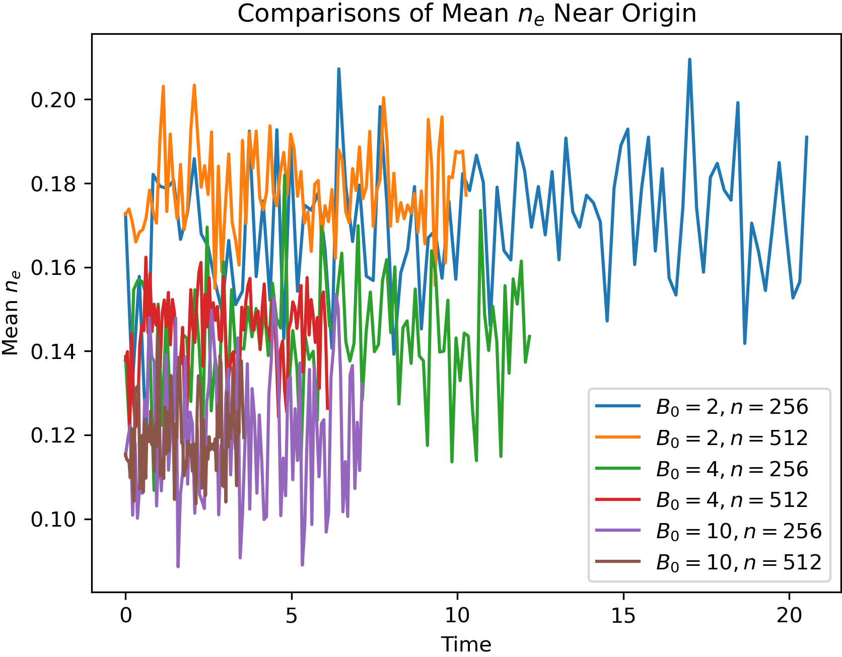
Figure 10: Electron density $n_{e}$ at the center for $B_{0}=2$, 4, and 10 using $256^{2}$ and $512^{2}$ grids for exact runs.

To the best of our knowledge, this is the first time 2D BGK mode solutions of a form similar to Eq. (5) have been confirmed with a kinetic simulation. This is remarkable in the sense that such solutions are fully nonlinear, self-consistent localized solutions of the Vlasov-Poisson system of equations, i.e., Eqs. (3) and (4). Moreover, this result also shows that there exists solutions that are stable over some ranges of parameters, at least with perturbations confined in the 2D plane, and up to rather long durations of the simulations. The stability study for more general perturbations using 3D PIC simulations is ongoing, and will be the subject of a later publication.

IV.2.3 Unstable Cases

Exact runs with $B_{0}\lesssim 1$ were unstable. Unstable modes can appear due to the bimodal velocity distribution as in Fig. 1. The instability manifests as radial arms in $n_{e}$ that rotate counterclockwise around the origin, as shown in Figs. 11; note that the electron flow is clockwise.

The fluctuations are especially visible in the azimuthal component of the electric field $E_{\phi}$, as in 12 and in the movies in the Supplementary Material. We thus identify these rotating fluctuations as electrostatic waves. The propagation appears as roughly co-rotating at first, and then either forms a spiral pattern as it fades away.

Spiral waves are clearly seen in the $n_{e}$ and $E_{\phi}$ movies for $B_{0}=0.25$, 0.5, and 1. For the $B_{0}=0.1$ case, the initial wave has many more arms than other cases (12 or more), but the co-rotation phase quickly ends with the almost total dissipation of the wave, obscuring any possible spiral phase and making analysis difficult.

For the $B_{0}=1$ case, the instability takes a long time ($t>100$) to appear, but the spiral wave lasts a long time, persisting until we had to stop the simulation at $t=433$. This case, as well as the $B_{0}=0.5$ case, has only four arms, while the $B_{0}=0.25$ case has between 6 and 8. Some of these arms are not present over the full range of $\rho$ for which there are unstable waves; rather, there appears to be bifurcations such that one arm can split into two when going radially outwards, as can be seen in Fig. 12. Generally, not all arms are of the same strength, suggesting a mixture of unstable modes instead of one single mode.

Given the spiral structure of the density fluctuations, the waves should also have $E_{\rho}$ fluctuations such that the wave has a component propagating outwards along the $\rho$ direction. The $E_{\rho}$ fluctuations are more difficult to see because $E_{\rho}$ from the background BGK mode is large compared with the fluctuations. We include one $E_{\rho}$ movie in the Supplemental Materials for the $B_{0}=1$ case to illustrate this point. In fact, the wave starts to have more apparent outward propagation when the spiral pattern emerges, and this could be the physical reason behind the formation of the spiral pattern.

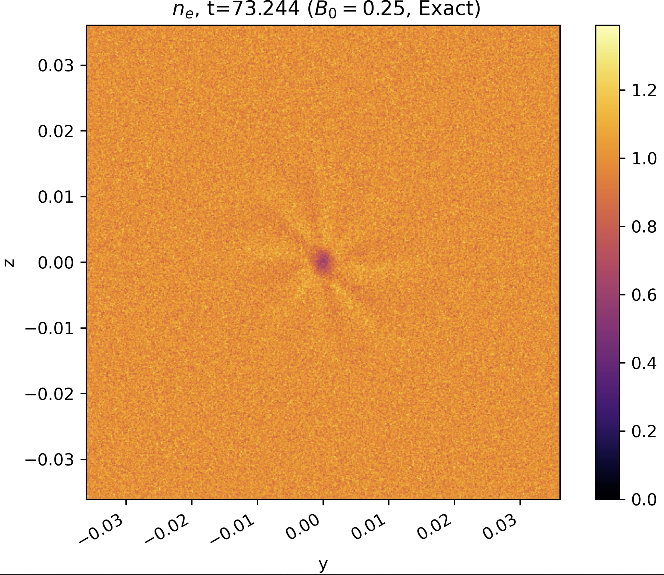
Figure 11: $n_{e}$ map for an exact $B_{0}=0.25$ run of resolution $512^{2}$ at the given time.

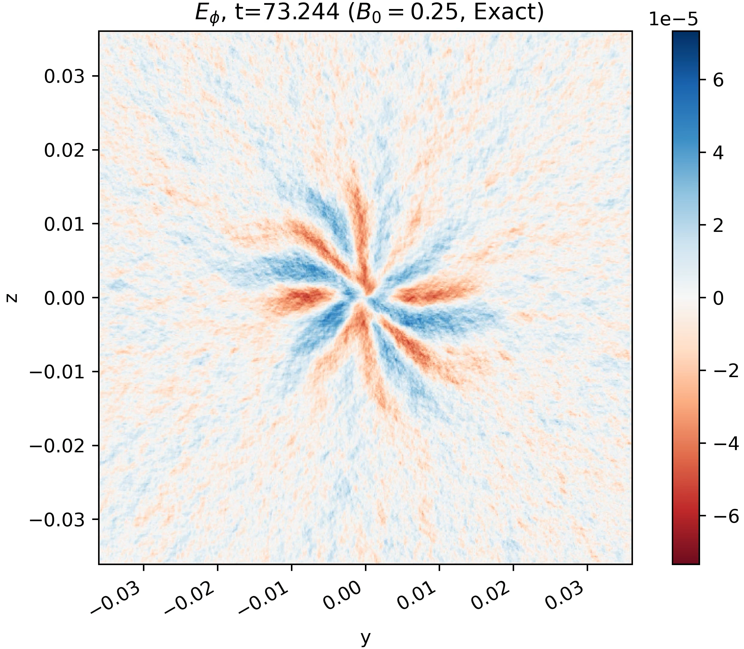
Figure 12: $E_{\phi}$ map for an exact $B_{0}=0.25$ run of resolution $512^{2}$at the given time.

IV.2.4 Post-Instability

It is observed that the electron density hole begins to fill as soon as the instability appears. This can be seen from the $n_{e0}$ vs. $t$ plots, e.g. Fig. 13 for cases with weak $B_{0}$ and Fig. 14 for cases with medium $B_{0}$.

These two figures are significantly different from corresponding figures from the moment runs, i.e., Figs. 4 and 5. The latter exhibit pulsation, while the former appear to follow logistic curves and saturate at a value below 1. This is clearly show in Fig. 15. We see that the growth of $n_{e0}$ starts near $t\sim 0$ for the $B_{0}=0.1$ and $0.25$ cases, while there may be a linear phase in the growth of $n_{e0}$ for the $B_{0}=0.5$ and 1 cases, as it takes some time for the instability to grow.

As far as our simulations can show, $n_{e0}$ apparently stabilizes at a value below 1 for these unstable cases. In other words, there is still an electron density hole after the initial hole decays, albeit one with an $n_{e0}$ closer to 1. The spike also seems to survive the instability. The snapshots of the exact $B_{0}=1$ run in Fig. 8 show such a state in the last two frames, while the second frame captures a glimpse of the radial arms. If an electron density hole truly does exist after the instability, it is unclear whether it would be in a stable time-steady state similar to the solutions described by Eq. (5).

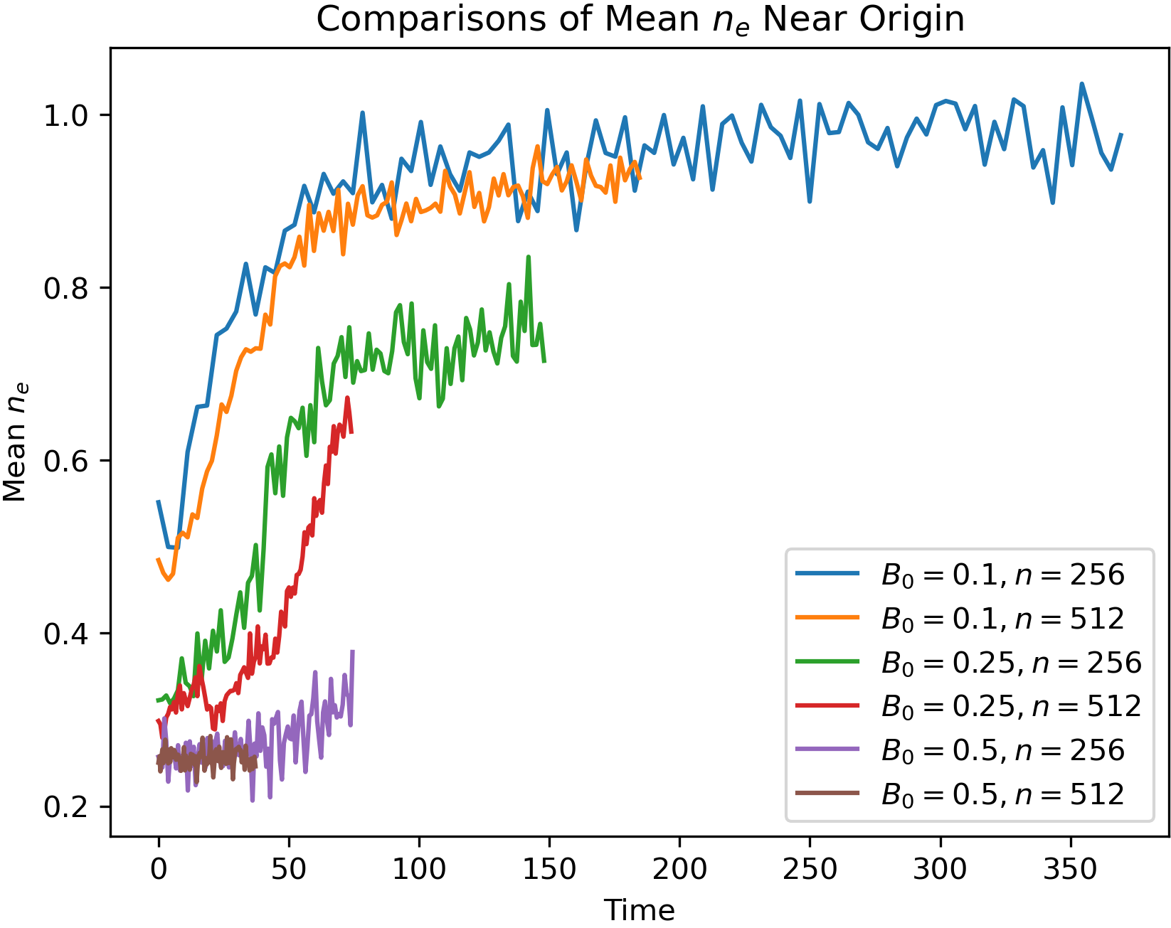
Figure 13: Electron density $n_{e}$ at the center for $B_{0}=0.1$, 0.25, and $0.5$ using $256^{2}$ and $512^{2}$ grids for exact runs.

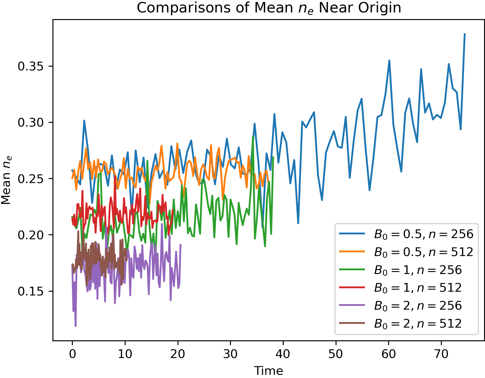
Figure 14: Electron density $n_{e}$ at the center for $B_{0}=0.5$, 1, and 2 using $256^{2}$ and $512^{2}$ grids for exact runs.

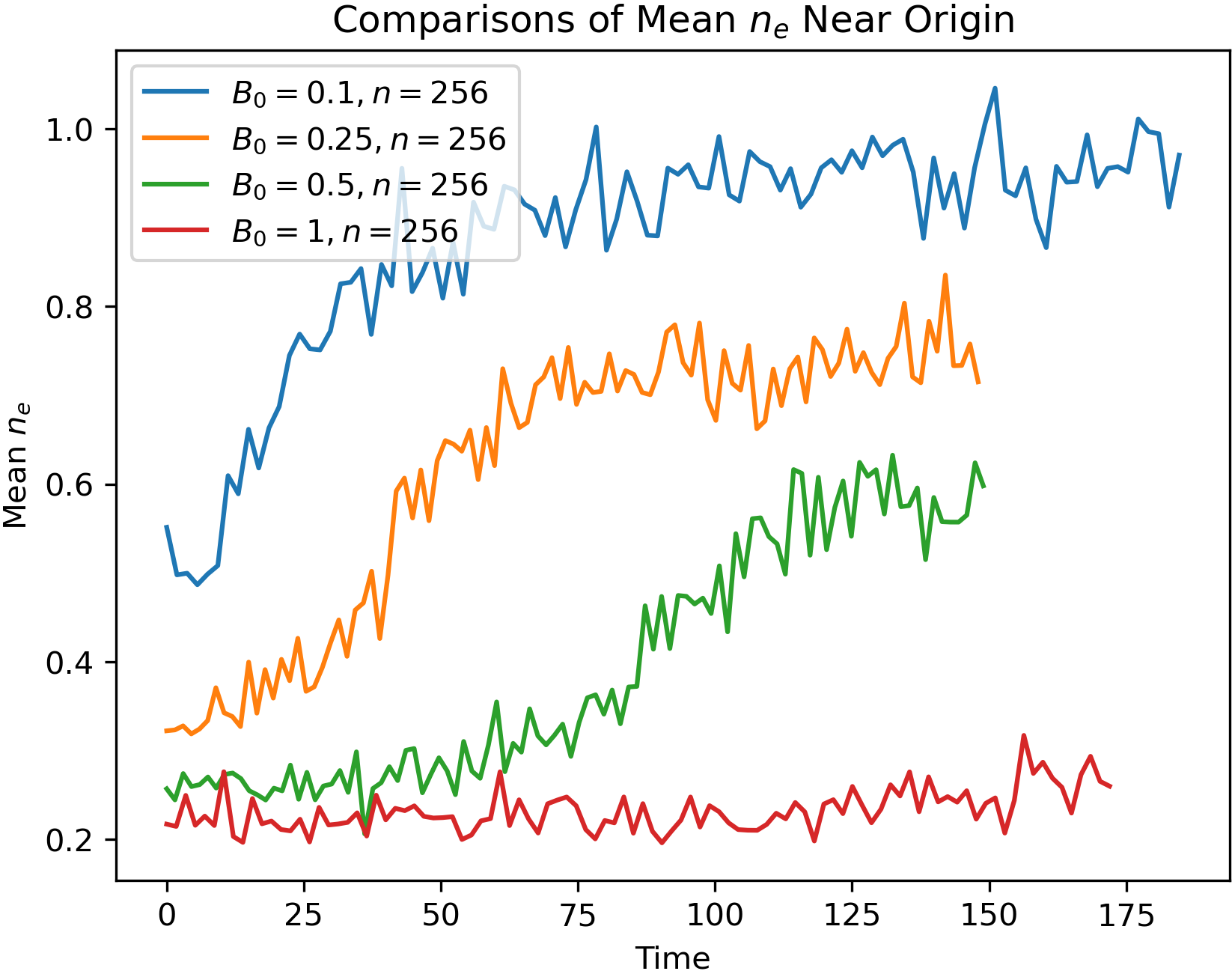
Figure 15: Electron density $n_{e0}$ at the origin for $B_{0}\leq 1$ using $256^{2}$ grids for exact runs. Higher-$B_{0}$ runs had to be extended multiple times to achieve such high times.

IV.2.5 Comments on Stability

It is unknown what critical value of $B_{0}$ separates stability from instability, since we have not simulated enough cases with different $B_{0}$. The apparent stability of high-$B_{0}$ runs indicates that such a value exists, and our limited number of cases suggest that it is around $B_{0}\sim 2$ for our choice of other parameters $h$ and $k$. The chosen form of the analytic BGK mode distribution shown in Eq. (5) implies that the critical value of $B_{0}$ depends on these parameters. For example, using a smaller value of $h$ for the same $B_{0}$ will make the distribution more Maxwellian, and a Maxwellian distribution is well known to be stable.

Due to limitations of space and scope, we omit a more thorough analysis of the observed instabilities, including numerical results and a comparison to a theoretical model. We will present such discussion in a separate publication instead.

IV.3 Scaling

Unstable runs, i.e., exact runs with low $B_{0}$, were somewhat affected by resolution. This was to be expected, since PIC simulations are inherently noisy, and it is likely that particle noise affects the evolution of the unstable configurations. Figure 16 lends credit to this idea by showing that the instability growth depends more on nicell than on the resolution. Importantly, although the total number of macroparticles affected the time for growth to begin, it significantly affected neither the growth rate nor the final $n_{e0}$ value. It seems that particle noise kickstarts the growth process, and more noise triggers it sooner.

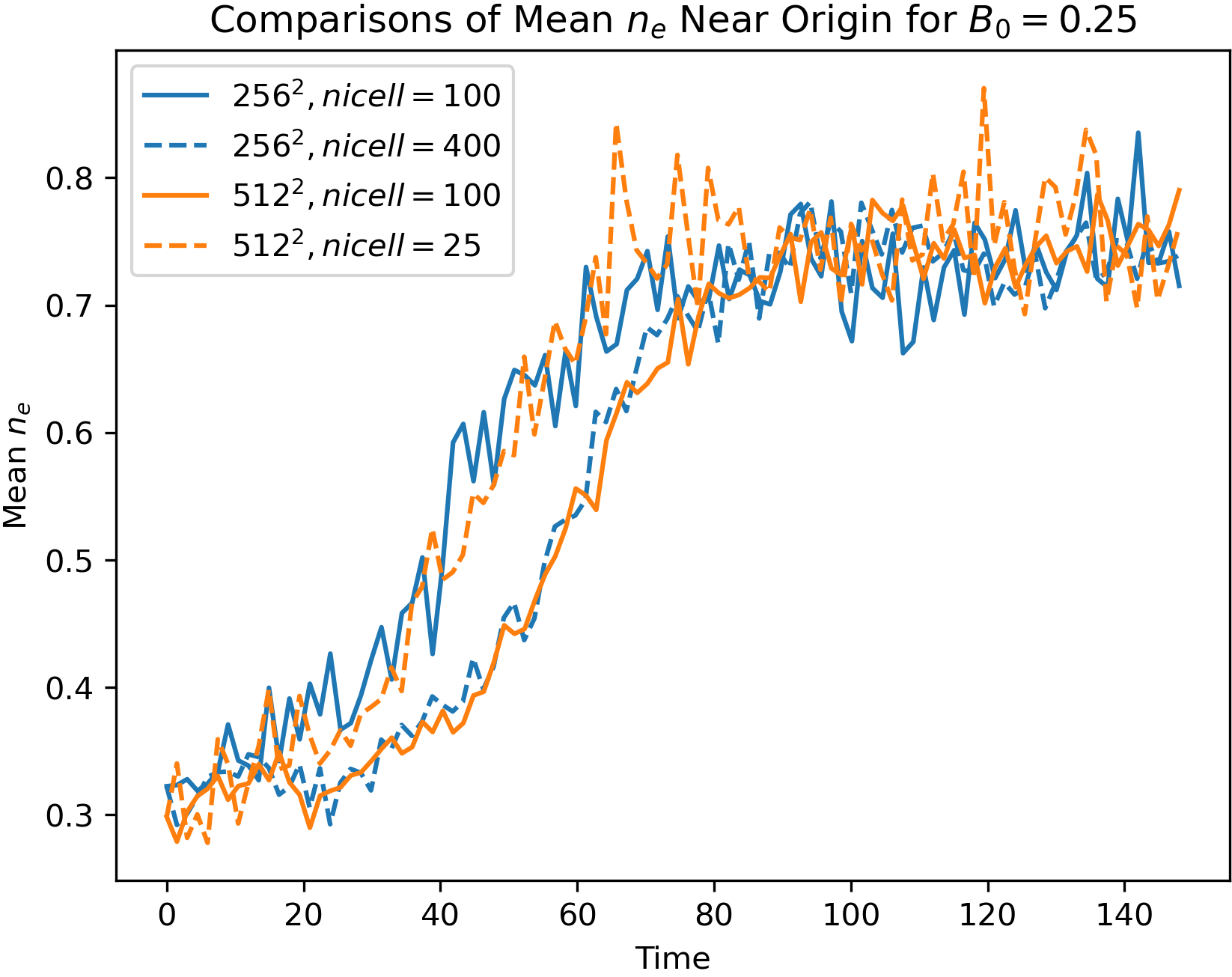
Figure 16: Comparing the effects of resolution and nicell on the growth rate of exact $B_{0}=0.25$ runs. Total number of electron macroparticles is $\texttt{nicell}*\text{number of cells}$.

For the most part, other runs did not appear sensitive to scaling. Noise was likely suppressed in high-$B_{0}$ exact runs, which were stable. As for moment and reversed runs, the deliberate perturbations would have dominated any noise. Plots similar to Fig. 16 were produced for these runs and showed convergence for all resolutions tested.

One possible exception is for cases with $B_{0}=0.1$. For such cases, the spike extends far from the origin while the hole itself stays small. Consequently, a large physical domain is needed to resolve the spike, so a high resolution is needed to resolve the hole. In fact, the central 4 cells used to calculate $n_{e0}$ almost cover the entire density hole of the $256^{2}$ run, so the method used to plot the time series $n_{e0}$ is not very accurate.

Overall, while we did not have time to perform an extensive scaling analysis, we are reasonably certain that even our $256^{2}$ runs were sufficiently resolved—again, with the possible exception of $B_{0}=1$. Certainly, our $2048^{2}$ runs were sufficiently resolved, and they exhibited the same qualitative behavior as our other runs.

V CONCLUSION AND DISCUSSION

With the development of a new method to input an analytic distribution as initial conditions (the “exact method”) in PSC, our simulations affirm the validity of Eq. (5) as a steady-state solution to the Poisson-Vlasov system of equations. This is the first time to our knowledge that such a solution has been validated using a kinetic code. The evidence of time-steadiness was further supported by contrasting exact runs with “moment” runs, which effectively served as a control. Moment runs were never as time-steady as their exact counterparts, even at high $B_{0}$ with resolutions of $2048^{2}$. Since solutions of the form of Eq. (5) are self-consistent, they may be useful as validation cases involving nonlinear physics for other kinetic codes, now that they are shown to be correct.

The validity of the time-steadiness of such solutions also shows that there exist 2D BGK modes that are stable for some ranges of parameters, under the restriction of 2D perturbations. We must therefore take more seriously the possibility that these structures exist in nature. To show this more conclusively, we will have to wait for more kinetic simulations in 3D, which we are working on currently.

Our PIC simulations also found that for our choice of parameters $h$ and $k$, solutions are stable in the large-$B_{0}$ limit, and unstable in the opposite limit. In particular, the instabilities were found to excite azimuthally-propagating electrostatic waves. These waves initially co-rotate, and can evolve into a spiral pattern as they start to decay.

The instability was also found to have the associated effect of filling the central electron density hole, although only partially: in every unstable case we ran, the electron density at the origin seemed to stabilize at a value less than 1. The resulting density hole may persist for a much longer period of time than the initial hole.

Moreover, except for very low values of $B_{0}$, the electron density holes in the moment (and even reversed moment) runs are only temporarily filled by pulsations. We have not followed the long-time evolutions of such cases, since doing so would require more computation time than we could spare. It would be of great interest to find out whether a generic electron density hole configuration would evolve to a new, stable hole configuration after instabilities and pulsations run their course, as we found with our weak-$B_{0}$ exact runs. If the answer to this question is affirmative, this would provide a general mechanism for 2D BGK modes to form, further strengthening the possibility that they may exist in nature.

V.1 Galactic Similarities

The excitation of spiral waves from the instability of the 2D BGK modes could be of interest outside of plasma physics—galactic dynamics, specifically. This is not because of the outward similarity of the spiral wave patterns to spiral galaxies, but because a collisionless plasma system and a stellar system are both described by the same equations: the Vlasov equation and the Poisson equation, with some sign changes to reflect the fact that the gravitational force between masses is always attractive, unlike electric forces. In fact, like BGK modes, galaxies can be regarded as kinetic equilibria of this system of equations. Binney and Tremaine (2008) The fact that the physics behind the formation of spiral galaxies is considered somewhat unsolvedBinney and Tremaine (2008) suggests that our observation of spiral waves excitation for unstable 2D BGK modes might provide some insight for that problem.

One might counter this suggestion by pointing out that our 2D solutions are actually tube-like when viewed in the 3D spatial domain, while a galaxy is a genuinely 3D object. However, one of us (CSN) has developed a “galactic disk” model of a 3D BGK mode, to be presented in a separate publication, in which the form of the distribution of the disk particle is very similar to that of the 2D BGK modes, i.e., Eq. (5). It will be shown that a galactic disk can in fact have very similar physics to a 2D system.

V.2 Future Work

The research presented in this paper is our first attempt at studying the stability of 2D BGK modes using PIC simulations. Therefore, we have started with the simplest cases, and have restricted the choices of parameters of the model, i.e., we kept $(k,h)=(0.4,0.9)$ fixed. As discussed in section IV.2.5, other choices of these parameters could change the stability boundary of the only parameter that we vary, i.e., $B_{0}$.

Additionally, we limited $v_{e}=c/1000$ to make sure that the theory can be meaningfully compared with simulations. In our future studies, we plan to relax such restrictions progressively. This would obviously require significant computational effort, and also more calculations as discussed in Section II.2. For example, a larger $v_{e}$ which is still non-relativistic would involve solving Ampère’s Law self-consistently alongside Eqs. (3) and (4) resulting in a BGK mode with nonuniform background magnetic field. Ng (2020)

One must also keep in mind that the form of the distribution given in Eq. (5) is just one of infinitely many possible choices. Thus, 2D BGK modes are really given by an unlimited number of parameters. While this is an intimidating prospect, we can list a few interesting and meaningful generalizations that we can study in the future:

1. choose a negative $h$ for an electric density “bump” instead of a hole at the center;

2. choose a very small $k$ such that the mode will have a non-uniform magnetic field, generated self-consistently by Ampère’s Law even with a small but finite $v_{e}/c$;

3. include the dependence on the axial component of the canonical momentum in the form of the distribution, such that the mode has an associate magnetic field that has a azimuthal component;Ng (2020)

4. include a background of ions that satisfies a Boltzmann distribution, and might not have the same temperature as the background electrons;

5. consider BGK modes comprising kinetic ions with ion distributions depending on canonical angular momentum, with Boltzmann or kinetic electrons;

6. and consider distributions with forms different from that of Eq. (5), such as with a linear dependence on $l$, instead of $l^{2}$, in the argument of the exponential function in the second term of the right-hand side.

Although this list is by no means exhaustive, it would clearly require a huge effort to address all the tasks properly, and cannot possibly be finished by our team alone. This discussion is simply to demonstrate the rich possibilities of different kinds of small kinetic structures, and it is likely that new and unexpected physics can come from some of them.

VI Supplementary Material

https://drive.google.com/drive/folders/12DLFK-kR7upP-wHh0V4Pjyc1Y3veVIah

References

- Bernstein, Greene, and Kruskal (1957) I. B. Bernstein, J. M. Greene, and M. D. Kruskal, “Exact nonlinear plasma oscillations,” Phys. Rev. 108, 546–550 (1957), https://doi.org/10.1103/PhysRev.108.546 .
- Ng and Bhattacharjee (2005) C. S. Ng and A. Bhattacharjee, “Bernstein-Greene-Kruskal modes in a three-dimensional plasma,” Phys. Rev. Lett. 95, 245004 (2005), https://doi.org/10.1103/PhysRevLett.95.245004 .
- Ng, Bhattacharjee, and Skiff (2006) C. S. Ng, A. Bhattacharjee, and F. Skiff, “Weakly collisional Landau damping and three-dimensional Bernstein-Greene-Kruskal modes: New results on old problems,” Physics of Plasmas 13, 055903 (2006), https://doi.org/10.1063/1.2186187 .
- Ng (2020) C. S. Ng, “Kinetic flux ropes: Bernstein-Greene-Kruskal modes for the Vlasov-Poisson-Ampère system,” Physics of Plasmas 27, 022301 (2020), https://doi.org/10.1063/1.5126705 .
- Ng, Soundararajan, and Yasin (2012) C. S. Ng, S. J. Soundararajan, and E. Yasin, “Electrostatic structures in space plasmas: Stability of two-dimensional magnetic Bernstein-Greene-Kruskal modes,” AIP Conference Proceedings 1436, 55–60 (2012), https://aip.scitation.org/doi/pdf/10.1063/1.4723590 .
- Germaschewski et al. (2016) K. Germaschewski, W. Fox, S. Abbott, N. Ahmadi, K. Maynard, L. Wang, H. Ruhl, and A. Bhattacharjee, “The plasma simulation code: A modern particle-in-cell code with patch-based load-balancing,” Journal of Computational Physics 318, 305–326 (2016).
- Tang (2020) H. Tang, “Two-dimensional Bernstein-Greene-Kruskal modes in a magnetized plasma with kinetic effects from electrons and ions,” M.S. Thesis, University of Alaska Fairbanks (2020).
- Binney and Tremaine (2008) J. Binney and S. Tremaine, Galactic Dynamics: Second Edition, (Princeton University Press, 2008).