An analysis of parton distributions in a pion with Bézier parametrizations

Abstract

We explore the role of parametrizations for nonperturbative QCD functions in global analyses, with a specific application to extending a phenomenological analysis of the parton distribution functions (PDFs) in the charged pion realized in the xFitter fitting framework. The parametrization dependence of PDFs in our pion fits substantially enlarges the uncertainties from the experimental sources estimated in the previous analyses. We systematically explore the parametrization dependence by employing a novel technique to automate generation of polynomial parametrizations for PDFs that makes use of Bézier curves. This technique is implemented in a C++ module Fantômas that is included in the xFitter program. Our analysis reveals that the sea and gluon distributions in the pion are not well disentangled, even when considering measurements in leading-neutron deep inelastic scattering. For example, the pion PDF solutions with a vanishing gluon and large quark sea are still experimentally allowed, which elevates the importance of ongoing lattice and nonperturbative QCD calculations, together with the planned pion scattering experiments, for conclusive studies of the pion structure.

I Introduction

The internal structure of hadrons, as a window on versatile aspects of strong interactions, is at the center of forefront studies of quantum chromodynamics (QCD) in the nonperturbative regime. New experiments will map internal composition of various hadron species in three dimensions across a broad range of QCD scales, including the perturbative/non-perturbative transition region [1, 2, 3]. The experimental developments are complemented by vigorous theoretical efforts to model the hadron structure using nonperturbative quantum-theoretical methods as well as lattice gauge theory [4, 5, 6].

Global phenomenological analyses of hadron scattering data serve as a bridge between experiment and theory. In these approaches, parametrizations of nonperturbative correlator functions quantifying the hadron structure are determined from a combination of hard-scattering experimental data and theoretical inputs. The most advanced global analyses are dedicated to determination of unpolarized parton distribution functions (PDFs) of nucleons and nuclei [7]. These analyses include multiloop hard-scattering contributions, up to the next-to-next-to-leading order (NNLO) in the QCD coupling strength $\alpha_{s}$, to assure accuracy and precision of the resulting PDFs. They also include sophisticated statistical machinery to evaluate various types of uncertainties.

Recently, the ever-evolving global analyses have been applied to study PDFs of pions [8, 9, 10, 11] within refined theoretical and methodological frameworks that supersede the earliest such analyses in Refs. [12, 13, 14]. In addition, fits of the pion PDFs in specific models have been proposed, such as the statistical model [15] (and references therein) or the light-front wavefunction formalism [16].

Phenomenological studies of pion PDFs draw attention in light of concurrent rapid developments in lattice QCD that quantitatively predict characteristics of the PDFs (flavor composition, Mellin moments, momentum fraction dependence, …) by computing matrix elements of bilocal current operators for the PDFs or related quantities [17, 18, 19, 20, 21, 22, 23, 24, 25, 26]. More broadly, the pion structure, while experimentally less accessible than the nucleon one, is studied extensively in QCD theory with the goal to elucidate how the pion’s two-body bound state emerges as a pseudo-Goldstone boson from the dynamical breaking of chiral symmetry. The pion structure is expected to hold clues to the symmetry-breaking mechanism responsible for the emergence of hadron masses, e.g. [27, 28, 29, 30, 31]. Such a mechanism may be most obvious for the pions, the lightest long-lived mesons, whose mass decomposition is influenced by the contribution coming from the current quark masses far less than the kaons and heavier mesons. The upcoming experiments will investigate the transition from this picture, valid at nonperturbative scales of 1 GeV or less, to another picture in terms of weakly interacting quarks and gluons, applicable in the multi-GeV energy range, for the pions and mesons in general.

Learning from the experimental observables about the pion’s primordial structure via PDF fits invariably relies on quantification of contributing uncertainties, and those arise from several generic classes of factors: experimental, theoretical, parametric, and methodological [7]. In this article, we address the uncertainty due to the choice of the functional forms for PDFs at the initial scale of QCD evolution – the type of uncertainty that has not been assessed systematically in the recent pion fits. Potentially significant, the parametrization uncertainty on the PDFs is not automatically reduced by increasing the event statistics or the order of the perturbative calculation. Its assessment requires dedicated techniques, whether the PDFs are approximated by polynomials, neural networks, or other functional forms. In the nucleon global fits, sampling over plausible functional forms was shown to contribute a large part of the total published uncertainty [32, 33]; its effect is especially evident in the kinematic regions with poor experimental constraints, as has been demonstrated e.g. in the fits utilizing the neural networks [34]. The estimation of the parametrization uncertainty is greatly simplified for typical QCD observables that depend only on a few leading PDF combinations. For such observables, one strives to learn the likely spread of PDFs from fitted data by repeating the analysis for a manageable collection of PDF parametrizations.

We have developed a C++ package Fantômas to parametrize a variety of nonperturbative correlator functions using polynomial shapes realized by Bézier curves. The Bézier parametrizations can approximate an arbitrary continuous function with desired accuracy as a consequence of the Stone-Weierstrass approximation theorem. That theorem carries the same significance for the polynomial functions as the universal approximation theorems [35, 36, 37] do for neural networks. The control parameters of the Bézier curves are nothing but the values of the PDFs themselves at user-specified control points. These parameters have a direct interpretation, in contrast to the free parameters of neural networks and traditional parametrization approaches. Those benefits of a Bernstein polynomial basis were taken advantage of in an early examination of structure functions [38]. Today, we know that the Bézier curve framework also serves to mitigate instabilities in the polynomial interpolation associated with the Runge’s phenomenon. It aims to make exploration of the parametrization dependence both interpretable and amenable for automation. It will be fully described in an upcoming publication.

We incorporated the Fantômas package into the public code xFitter [39] and employed it to gain insights about the pion PDFs, starting from and then expanding the recent analysis of pion PDFs published in [9]. We determine these PDFs at the next-to-leading order (NLO) accuracy by fitting pion-nucleon Drell-Yan (DY) pair production (largely constraining the quark PDFs), prompt photon production, and newly added data from HERA leading-neutron production in deeply inelastic scattering (DIS) (constraining the gluon PDF at $x<0.1$). We fit the PDFs using several trial functional forms and produce a final ensemble of Hessian error PDFs by combining the PDFs from the trial fits using the meta-PDF combination method [40]. The resulting ensemble of pion error PDFs is named “FantoPDF.”

Exploration of pions, with their simple valence partonic structure and the central role played by chiral symmetry breaking in their formation, raises important physics questions that can be elucidated in new experiments [4, 41, 42]. How does the pion’s valence quark PDF depend on the partonic momentum fraction $x$? How large is the pion’s gluon PDF at QCD scales of about 1 GeV? Answering these questions requires one to thoroughly explore and interpret the PDF parameterization dependence. The Bézier parametrizations are designed for this purpose.

For example, the shape of the valence PDFs in the asymptotic limit $x\to 1$ reflects several factors entering at disparate energy scales. Dynamical chiral symmetry breaking generically manifests itself as broadening of the pion distribution amplitude and the pion quark PDF at a low hadronic scale. Kinematic constraints in the quasielastic limit lead to a power-law fall-off of structure functions and PDFs at $x\to 1$ as a function of the number of spectators and helicity combinations in low-order Feynman diagrams. Perturbative QCD radiation further suppresses the PDFs at the largest momentum fractions and high scales as a consequence of the radiative energy loss from the fastest partons inside the hadron.

Discrimination among these factors based on the empirical data has been challenging, not the least because of the parametrization dependence. Various lattice calculations confirm a broad, nearly flat pion distribution amplitude at low scales [43, 44], and a broad valence pion PDF [18, 19, 21, 20, 45, 46, 47]. These features predicted from first principles can be compared against the central PDFs and uncertainty bands of the FantoPDF ensemble in lieu of directly comparing against data. The impact of the parametrization uncertainty on the derived quantities, such as the moments and logarithmic derivatives of the PDFs, can be examined. By trying a variety of flexible functional forms, we suppress the bias present in the case of using one fixed form. Many functional behaviors (e.g., given by different polynomials) are consistent with the discrete data – this functional mimicry emphasized in our recent study [48] stands in the way of determining the unique analytical form of the PDFs from the discrete data sets. The functional mimicry also holds a positive aspect, namely that polynomial functions generated on the fly can realize a wide range of functional behaviors.

On the side of the data analysis, the available hard-scattering experimental data on the pion have been collected in the 1980’s and has only a limited constraining power on the PDFs, as has been already emphasized in 1990’s [12, 13, 14]. Restrictive parametrization forms fail to capture these limitations when comparing against nonperturbative QCD methods, not to mention the so-far ignored uncertainties due to the flavor composition of the quark sea and nuclear PDFs. We make a step toward obtaining trusted uncertainty estimates.

Section II introduces the key mathematical formalism of PDF functional forms based on Bézier curves. Section III sets up the characteristics of the global analysis that leads to the FantoPDF for the pion in Section IV. The results are discussed in Section V. Then we compare the FantoPDF results with previous global analyses (Section VI) and lattice evaluations (Section VII), to finally conclude in Section VIII.

II Parton distributions parameterized by Bézier curves

II.1 Motivation

The simplest parameterizations of the hadron PDFs at the initial scale $Q_{0}$ of the DGLAP evolution can be of a “baseline” functional form,

$$x\,f_{i}(x,Q_{0}^{2}) = A_{i}x^{B_{i}}(1-x)^{C_{i}}\equiv F_{i}^{car}(x)\ ,$$ (1)

where $i$ runs over all partons. The normalization coefficients $A_{i}$ are chosen to satisfy the number and momentum sum rules. The powers $x^{B_{i}}$ and $(1-x)^{C_{i}}$ capture the Taylor series expansions in the limits $x\to 0$ and $1$. We call this form a carrier function $F_{i}^{car}(x)$.

To introduce more freedom at $x$ away from 0 or 1, we multiply the carrier function $F_{i}^{car}(x)$ by another function $F_{i}^{mod}(x)$ that we call a modulator:

$$x\,f_{i}(x,Q_{0}^{2}) = F_{i}^{car}\times F_{i}^{mod}\ .$$ (2)

The modulator function is taken to be

$$F_{i}^{mod}\left(x;{\cal B}^{(N_{m})}\right) = 1+{\cal B}^{(N_{m})}(y)$$ (3)

in terms of a polynomial ${\cal B}^{(N_{m})}(y)$ of order $N_{m}$ and argument $y\equiv y(x)$, where $y(x)$ is a stretching function to be defined below. [In the simplest realization, $y=x$.] The baseline parametrization of Eq. (1) is recovered for ${\cal B}^{(N_{m})}=0$.

In our methodology, the ${\cal B}$ polynomial is chosen to be a Bézier curve, which has been extensively used in various applications, as it provides a flexible functional interpolation. A Bézier curve is defined as

$${\cal B}^{(N_{m})}(y)=\sum_{l=0}^{N_{m}}c_{l}\ B_{N_{m},l}(y)$$ (4)

by introducing a basis of Bernstein polynomials,

$$B_{N_{m},l}(y)\equiv\left(\begin{matrix}N_{m}\\ l\end{matrix}\right)y^{l}(1-y)^{N_{m}-l}\ ,$$ (5)

where the $\binom{N_{m}}{l}$ is a binomial coefficient.

Polynomial functional forms of the type of Eq. (2) are widely used in global analyses. The CTEQ-TEA group builds their modulator function from Bernstein polynomials [32], while the MSHT group employs Chebyshev polynomials [49]. Once the degree $N_{m}$ of the polynomial is fixed, either polynomial basis results in the same modulator. The central advantage of the Bézier curve is that the numerical coefficients of the polynomial – $c_{l}$ in Eq. (4) – are computed from the values of the modulator function at a few user-specified values of $x$, or control points (CPs), instead of being fitted directly. These values of the modulator function become the free parameters. When the modulator is constructed this way using the Bézier curve with $y(x)$ as an argument, we call the whole $xf_{i}(x,Q_{0}^{2})$ in Eq. (2) a metamorph to distinguish it from the other possible forms.

While the Bézier representation is algebraically equivalent to the traditional polynomial forms, it helps to control numerical correlations among the parameters, which is critical for uncertainty quantification. For example, the sign-indefinite orthogonal polynomials generally require significant cancellations between coefficients $c_{l}$ to obtain a positive PDF. This is not an issue with the Bézier curves. Another advantage is that the power $N_{m}$ of the polynomial can be raised or lowered by adding the control points to the existing parametrization or deleting them. When doing so, the already existing control points are not affected; at this instance, flexibility of the parametrization can be raised or lowered while keeping the input function as is.

Discrete data do not uniquely fix the degree of a continuous polynomial, reflecting the functional mimicry of polynomial interpolations explored in Ref. [48]. Functional mimicry is the observation that polynomials of different degrees can yield virtually identical $\chi^{2}$ over the fitted $x$ range (leading to $f^{m}(x)=f^{\prime m^{\prime}}(x)$ at the fitted points numerically, with $m\neq m^{\prime}$), while at the same time these polynomials produce drastically disparate extrapolations outside of the fitted range. Mimicry prevents us from extracting a unique polynomial power of the PDFs in an asymptotic $x$ limit (either $x\to 0$ or $1$); the phenomenological consequences for the pion PDFs will be discussed in Section V.

To decouple the flexibility at intermediate $x$ from the asymptotic behaviors at $x\to 0$ or $1$, we introduce a stretching function $y(x)$ such that $F_{i}^{mod}(x)\to 1$ in either asymptotic limit. The other role of $y(x)$ is to aid in the approximation of typical PDF shapes, notably the transition from the approximately logarithmic dependence on $x$ at $x\ll 1$ to the approximately linear one at $x\sim 1$.

In summary, the metamorph construction decomposes $xf_{i}(x,Q_{0}^{2})$ into a carrier $F_{i}^{car}$ and modulator $F_{i}^{mod}$. The carrier can be of a standard form in Eq. (1) or another suitable form. With a judicious choice of $y(x)$, which we normally do not vary during the fit, the carrier parameters $B_{i}$ and $C_{i}$ control the asymptotic limits $x\to 0$ and $1$, respectively. The control points in the modulator determine deviations of the PDF from the carrier at intermediate $x$. The placement of control points can be automated. Correlations between the parameters of the carrier and modulator are reduced. In the next subsection, we describe the technical realization of the metamorph, including the calculation of $c_{l}$ coefficients and the stretching function we employ.

II.2 Technical realization

II.2.1 Computing Bézier coefficients

In constructing our polynomials, we will rely on the unisolvence theorem stating that the coefficients of a polynomial ${\cal B}^{(N_{m})}(y)$ of degree $N_{m}$ can be computed exactly given a vector ${\underline{P}}\equiv{\cal B}^{(N_{m})}(y_{i})$ for $y_{i}=y(x_{i})$ at $N_{m}+1$ control points $x_{i}$ [48]. We utilize a notation in which $S$ (no underline), $\underline{V}$, and $\underline{\underline{M}}$ denote a scalar, an $(N_{m}+1)$-dimensional vector, and an $(N_{m}+1)\times(N_{m}+1)$ matrix. Hence, the Bézier curve ${\cal B}^{(N_{m})}(y)\equiv{\cal B}$ in Eq. (4) can be derived in a matrix form in various ways [50, 51], such as

$${\cal B}={\underline{Y}}^{T}\cdot\underline{\underline{M}}\cdot{\underline{C}},$$ (6)

where $\underline{Y}\equiv\{y^{k}\}$ is a vector whose entries are increasing powers of $y$ (with $k=0,\ ...,\ N_{m}$), $\underline{\underline{M}}$ is an $(\!N_{m}\!+\!1\!)\times(\!N_{m}\!+\!1\!)$ matrix containing combinations of binomial coefficients, and $\underline{C}$ contains Bernstein polynomial coefficients, $\{c_{l}\}$. From this relation, we further find that

$${\underline{P}} = {\underline{\underline{T}}}\,\cdot{\underline{\underline{M}}}\,\cdot{\underline{C}},$$ (7)

where we introduced a matrix $\underline{\underline{T}}$ constructed from powers $y^{k}$ with $k$ ranging between 0 and $N_{m}$. The matrices $\underline{\underline{M}}$ and $\underline{\underline{T}}$ are given explicitly in [48]. The coefficient vector $\underline{C}$ is then obtained as

$$\underline{C}=\underline{\underline{M}}^{-1}\cdot\underline{\underline{T}}^{-1}\cdot{\underline{P}}.$$ (8)

II.2.2 Fixed and free control points

To initialize the metamorph function $F_{i}^{car}(x;A_{i},B_{i},C_{i})\,\left(1+{\cal B}^{(N_{m})}(y)\right)$ at the beginning of the fit, we provide the initial coefficients $A_{i,0}$, $B_{i,0}$, $C_{i,0}$ in the carrier and vector $\underline{P_{0}}$ of the initial polynomial’s values at control points ${y_{i}}$. During the fit, we update the carrier parameters as

$$B_{i}=B_{i,0}+\delta B_{i},\quad C_{i}=C_{i,0}+\delta C_{i},$$ (9)

where the increments $\delta B_{i}$, $\delta C_{i}$ are varied by the minimization routine. We also vary some normalizations $A_{i}$, while other normalizations are computed using the sum rules. As for the components $P_{i}$ of ${\underline{P}}$ in the modulator, we vary them in a similar way ($P_{i}=P_{i,0}+\delta P_{i}$) at free control points or keep them constant ($P_{i}=P_{i,0}$) at fixed control points. For instance, for a $j$-th control point we may decide to keep $P_{j}=0$, so that the whole $xf(x,Q^{2})$ reduces to the carrier at $x=x_{j}$.

We can increment the polynomial degree $N_{m}$ by inserting a control point at some $x=x_{N_{m}+1}$. As the initial $P_{N_{m}+1,0}$ at the new point, we can either choose ${\cal B}^{(N_{m})}(y_{N_{m}+1})$ to retain the modulator value from the $N_{m}$-th degree polynomial, or set $P_{N_{m}+1,0}$ to any other value, for example, $P_{N_{m}+1,0}=0$.

II.2.3 The stretching function

In the current implementation, we choose a stretching function of the form $y=(g(x))^{\alpha_{x}}$, with $\alpha_{x}>0$ and with

$$g(x)\equiv\frac{1}{\left(\frac{1}{x^{6}+x_{\rm min}^{6}}+\frac{1-x_{\rm max}^{6}}{x_{\rm max}^{6}}\right)^{1/6}}$$ (10)

dependent on two constant parameters, $x_{\rm min}$ placed to the far left from the fitted interval of $x$, and $x_{\rm max}$ placed to the far right. It is easy to see that $g(x)\to x_{\rm min}$ when $x\ll x_{\rm min}$, and similarly $g(x)\to x_{\rm max}$ when $x\gg x_{\rm max}$. For $x_{\rm min}\lesssim x\lesssim x_{\rm max}$, $g(x)$ essentially coincides with $x$. The purpose of $g(x)$ is to turn off smoothly the modulator in the asymptotic intervals $0<x<x_{\rm min}$ and $x_{\rm max}<x<1$. Indeed, we can place two fixed control points with $P_{0}=P_{1}=0$ at $x_{0}=x_{\rm min}$ and $x_{1}=x_{\rm max}$. This choice forces $xf_{i}(x,Q^{2})=F_{i}^{car}(x)$ at $x\ll x_{\rm min}$ and $x\gg x_{\rm max}$, i.e. the PDF is asymptotically pinned to the carrier.

In the intermediate $x$ range, we can further rescale $y$ with respect to $x$ using the $\alpha_{x}$ power to redistribute the flexibility of the polynomial over the $x$ subranges. A possible choice $\alpha_{x}=0.3-0.5$ helps to capture the fast growth of a PDF at $x<0.1$ and slower dependence at $x>0.1$.

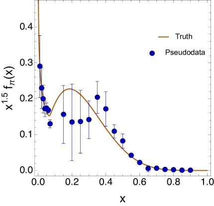
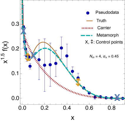
Figure 1: Illustration of a fit by a metamorph. (a) An ensemble of data points is generated by random fluctuations around a “truth” function constructed from piecewise polynomial interpolations. (b) After minimization of the $\chi^{2}$ between data and theory, the carrier function (short-dashed red curve) has varied and the values of all control points have been shifted, helped by the modulator, i.e., the Bézier curve. The “fixed” CPs (blue crosses) lie on the updated carrier function. The free CPs (golden arrows) can deviate from it. The final result is the long-dashed cyan curve, labeled “Metamorph”. It better approximates the data than the carrier only. This example is given for $N_{m}=4,\,\alpha_{x}=0.45$.

II.3 An illustration of aleatory and epistemic uncertainties

To demonstrate versatile features of the metamorph approach and to validate its C++ implementation, we implemented it in a Mathematica notebook [52] and tested it first by reproducing the coefficients of the Bernstein polynomials in CT18 NNLO parametrizations [32] by fitting the whole $xf_{i}(x,Q_{0}^{2})$ by metamorphs.

Figure 1 illustrates these features in a fit of generated fluctuating one-dimensional data in Mathematica. In Fig. 1(a), we generated such data by random fluctuations around a “truth” function (solid ocher curve), which in this specific example is given by a union of several piecewise polynomial curves. The goal is to fit the data with the metamorph methodology and compare it with the (known) truth. If the fitted function consists only of the carrier as in Eq. (1), the fit generally has a difficulty in fitting dip-bump structures like the one seen at $x=0.05-0.3$. Therefore, after fitting the data with the carrier only as a first estimate, we attach a modulator using two fixed control points at $x_{\rm min}=10^{-3}$ and $x_{\rm max}=0.9$, which are indicated by crosses in Fig. 1(b).

We then have freedom to choose, in accordance with the size and shape of the data [7], the degree $N_{m}$ of the modulator polynomial, the $x$ positions of $N_{m}+1$ control points, and the stretching parameter $\alpha_{x}$. We also can vary the style of the fit by keeping some parameters free or fixed. For example, the carrier parameters $B_{i}$ and $C_{i}$ could be held constant just like the preprocessing factors adopted by NNPDF [53], or they could be fitted together with the modulator, as other groups do.

In the example in the right subfigure, we selected $N_{m}=4$, $\alpha_{x}=0.45$ and added two variable control points at $x=0.05$ and 0.5 (indicated by the arrows), as well as a fixed control point that pins $xf(x)$ to the carrier at $x=0.1$. We varied both the carrier and control points and obtained a best-fit metamorph curve (long-dashed cyan), which is the product of the updated carrier function (short-dashed red curve) and the Bézier modulator curve.

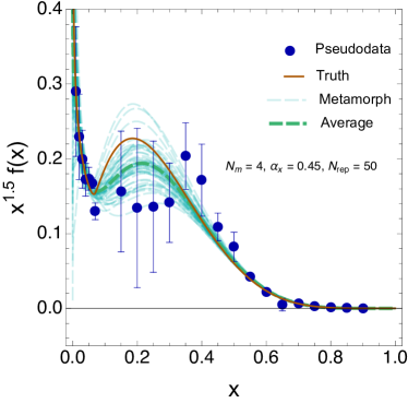
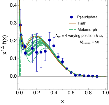
Figure 2: The Fantômas technique illustrated by applying the bootstrap (or importance) sampling on the data (upper plot) or the Fântomas methodology, that consists in sampling over representative choices for the CPs and the scaling factor $\alpha_{x}$ (lower plot). The resulting uncertainties are displayed in cyan (bootstrap) and green (parameter-space sampling).

The ultimate purpose for the metamorph methodology is to streamline quantification of uncertainties. Once a central fit has been determined, say, the long-dashed cyan curve of Fig. 1, its full statistical meaning is obtained through the propagation of the two classes of uncertainties: the aleatory and epistemic ones. The aleatory class in this case propagates from stochastic fluctuations of data. In the upper plot of Fig. 2, we estimate the aleatory uncertainty using the bootstrap method, one of the possible error propagation techniques. Also known as resampling or importance sampling, it involves generating $N_{\rm rep}=50$ replicas of the same data set by fluctuating the central data values according to their respective standard deviations. Each replica of the data is fitted by a respective metamorph (a light cyan curve in the upper plot of Fig. 2); their (unweighted) average is plotted here in green. The curves obtained after bootstrapping all correspond to the same metamorph settings (here $N_{m}=4,\ \alpha_{x}=0.45$, unvaried positions of CPs). The curves are superimposed on one replica of the data considered earlier. While each curve gives a good fit to their corresponding fluctuated replica, they at the same time give increasingly worse fits to the rest of the replicas when the number of parameters increases. This loss of generalizability of the PDF models can be partly mitigated by cross-validation (not done in our toy example). A single bootstrapped replica does not present a good fit to the averaged data, while their mean (the green line) usually does [54].

To estimate the epistemic uncertainties for some replica of data, it is necessary to sample over the space of models, which in the case of the metamorphs means the sampling over the settings to investigate a large collection of polynomials [33]. The lower plot in Fig. 2 shows a bundle of $N_{\rm curves}=50$ metamorph fits done on the same replica of data, now varying the positions and types of control points, as well as the stretching power $\alpha_{x}$. The degree of the polynomial, here set to $N_{m}=4$, can also be varied. The bundles in the upper and lower plots are not the same: bootstrapping of the data does not sample over the settings of the model and analysis. The total uncertainty can be estimated by combining the curves from both sources, which can be done using the METAPDF [40] or another method for combination of the PDF uncertainties. We will use this strategy to combine the experimental (aleatory) and parametrization (epistemic) uncertainties in the analysis of real pion data in the subsequent sections.

II.4 Implementation of metamorph in xFitter

In parallel with the Mathematica implementation, we have developed a C++ package Fantômas with the metamorph parametrizations, which was then incorporated into the xFitter fitting program [55, 39, 56, 57]. Just like the other standard parameterizations available in the PDF library pdfparams of xFitter, the metamorph functions can be used for any flavor of choice.

In contrast to the standard parametrizations, the metamorph parameterization requires the user to provide positions and types of control points, as well as parameters of the carrier and the stretching functions. All these parameters are stored in a dedicated steering card file, which is sufficient for reproducing the metamorph parameterizations between the fitting runs. The steering card also records the initial values of the modulator at the free control points. To simplify manipulations with the control points, Fantômas treats the shifts from the initial values at control points as free parameters. The shifts are varied to minimize the $\chi^{2}$. An updated Fantômas steering card is produced at the end of each fitting run.

Several options in the Fantômas module control the flexibility of the metamorphs. One option allows the carrier function, Eq. (1), to be fixed ($\delta B_{i}=\delta C_{i}=0$) or varied during the minimization process. An initial guess for the carrier parameters can be obtained by running an $N_{m}=0$ fit first, from which the obtained best-fit carrier parameters can be retained while increasing the degree of ${\cal B}^{(N_{m})}$.

An alternative strategy, which we employed in some candidate fits of the pion PDFs, is to allow free carrier parameters and fix $F^{mod}(x)=1$ at $0<x\ll x_{\rm min}$ and $x_{\rm max}<x<1$, as explained in Sec. II.2.3. Guidelines on the usage of the Fantômas environment in xFitter will be given in a separate publication that will accompany the public release of the C++ module and Mathematica notebook [58].

II.5 Placing of control points and Runge’s phenomenon

Control points are a crucial aspect of the metamorph not just because their positions $x_{i}$ can leverage the space of solutions by spanning more functional forms. Strategic placing of the control points prevents the instability in the interpolation when using a high-degree polynomial, also known as the Runge’s phenomenon. In Eq. (8), the instability arises when matrix $\underline{\underline{T}}$, the only part that depends on spacing of control points in $y$, has a vanishing determinant. This tends to happen, e.g., with equidistant spacing of control points and $N_{m}$ above 5-10, or when two control points are too close.

The Fantômas code computes the condition number for $\underline{\underline{T}}$ according to the Frobenius matrix norm. Together with a small ${\rm det}\,\underline{\underline{T}}$, a large condition number is another indicator that flags the likely polynomial instability. Users should seek to minimize this metric by setting up a well-behaved matrix $\underline{\underline{T}}$. This is achieved by taking advantage of the metamorph parameters, e.g. the stretching power $\alpha_{x}$.

With the typical choices we tested, the Bézier curve representation stabilizes interpolation with $N_{m}$ as high as 15-20. Such range of $N_{m}$ is entirely sufficient for the current phenomenology, as even the most precise nucleon PDF fits like CT18 and MSHT20 introduce at most about 30 effective degrees of freedom divided among all PDF flavors.

III Setup of the global analysis of the pion PDFs

III.1 Pion PDFs within the Bézier framework

In contrast to the extensively studied proton PDFs, only a few PDF fits have investigated the charged pion PDFs. The most recent analyses of this kind are done with modern fitting frameworks, e.g. developed by JAM (in a Monte-Carlo framework with Bayesian statistics [8, 11, 10]) and xFitter (in a Hessian framework [9]) groups. These investigations employed fixed polynomial forms with few parameters and reported negligible improvements in $\chi^{2}$, the figure of merit, when trying more flexible functional forms.

In anticipation that there may be significant parametrization dependence, the following sections extend the xFitter framework to include more general parametrizations for the initial PDFs using Bézier curves. Flexible functional forms are necessary to ensure proper sampling of the full space of solutions; this has been shown to affect uncertainty quantification for large-dimensional spaces [33]. While the parameter space for the pion PDF is arguably smaller than that of the proton, the extrapolation regions are spanned differently; gaps in the data coverage at small ($x\ll 0.1$) and intermediate ($x\sim 0.1$) momentum fractions require PDF parametrizations permitting enough variation within the gaps, not only at $x\to 0$ or $1$. Bootstrapping with fixed functional forms alone does not capture the extra uncertainty in the gap regions, as was observed e.g. in studies with hybrid fitting frameworks even for a small data ensemble [59, 60].

We work at the next-to-leading order (NLO) in the QCD coupling strength $\alpha_{s}$ and assume the same flavor composition of pion PDFs at the initial scale $Q_{0}^{2}=1.9\mbox{ GeV}^{2}$ as in the xFitter study [9]. In addition to the gluon PDF $g(x)$, we introduce the total valence and sea quark distributions, $V(x)$ and $S(x)$, and determine the PDFs for individual flavors on the assumptions that the PDFs for the two constituent (anti)quarks are the same in $\pi^{+}$ and $\pi^{-}$, and the light quark sea is flavor-blind:

$$u^{\pi^{+}}=\bar{d}^{\pi^{+}}=\bar{u}^{\pi^{-}}=d^{\pi^{-}}=V/2+S/6,$$ (11)

$$\bar{u}^{\pi^{+}}=\bar{d}^{\pi^{-}}=s^{\pi^{\pm}}={\bar{s}}^{\pi^{\pm}}=S/6.$$ (12)

Note that a priori $V(x)$ is not positive-definite. Using the above symmetries, we can compute all PDFs from three independent distributions, ${q=\{V,S,g\}}$, with each given by a metamorph functional form

$$x\,f_{i}(x,Q_{0}^{2})=A_{i}x^{B_{i}}(1-x)^{C_{i}}\left[1+{\cal B}^{(N_{m})}(y(x))\right].$$ (13)

Among the three PDF normalizations, $A_{V}$ is fixed by the valence sum rule. Depending on the candidate fit, we choose either $A_{S}$ or $A_{g}$ to be independent and find the third normalization from the momentum sum rule for $\langle xf\rangle=\int_{0}^{1}xf(x)\ dx$,

$$\langle xV\rangle+\langle xS\rangle+\langle xg\rangle=1.$$ (14)

In particular, we find that the gluon momentum fraction $\langle xg\rangle$ can be zero according to the data. Exploring such solutions with the xFitter program is most feasible when we choose $A_{g}$, rather than $A_{S}$, to be independent.

The metamorph parametrizations in Eq. (13) can be compared against the ones in the xFitter study [9]:

$$x\,V(x,Q_{0}^{2}) = A_{V}\,x^{B_{V}}(1-x)^{C_{V}},$$

$$x\,S(x,Q_{0}^{2}) = \frac{A_{S}}{B\left(B_{S}+1,C_{S}+1\right)}\,x^{B_{S}}(1-x)^{C_{S}},$$

$$x\,g(x,Q_{0}^{2}) = A_{g}\,(1+C_{g})\,(1-x)^{C_{g}}.$$ (15)

Here, the Euler-Legendre beta function $B(B_{S}+1,C_{S}+1)$ equates the momentum fraction $\langle xS\rangle$ of the sea quarks directly to $A_{S}$, taken to be independent.

At $Q$ scales above the charm and bottom masses, $m_{c}=1.43$ GeV and $m_{b}=4.50$ GeV, the charm and bottom PDFs are included in the DIS coefficient functions with mass dependence using the modified Thorne-Roberts scheme [61].

III.2 Selection of data

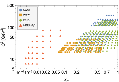
Figure 3: Kinematic coverage in $x_{\pi}$ and $Q^{2}$ of the Drell-Yan, prompt photon and leading-neutron DIS data used in this work.

The xFitter pion PDFs were determined from the analysis of Drell-Yan (DY) pair production by $\pi^{-}$ scattering on a tungsten target by E615 (140 data points) [62] and NA10 (140 data points) [63], as well as prompt-photon ($\gamma$) production in $\pi^{-}$ and $\pi^{+}$ scattering on a tungsten target by WA70 (99 data points) [64]. [See Ref. [9] for details on the data selection.] The kinematical coverage of those data is most sensitive to the pion PDFs at large $x$ values, as shown in Fig. 3. DY processes are most sensitive to valence distributions, with the gluon contributing mainly through the DGLAP evolution. The prompt-photon data provide additional constraints on the gluon distribution above $x\gtrsim 0.1$.

The data coverage did not allow the xFitter analysis to separate the quark sea ($S$) and the gluon ($g$) PDFs at $x<0.1$. To remedy the entanglement of the sea and gluon distributions, we followed the proposal of the JAM collaboration to analyze pion DIS data from leading-neutron (LN) processes [65, 8]. In such processes, the initial-state pion emerges nearly on its mass shell from a proton-neutron elastic transition. A flux factor modeling that $\pi PN$ transition is convoluted with the DIS structure function that is of interest here.

This idea was originally explored at HERA [66, 67, 68]. The kinematic variables for the DIS process include $x_{Bj}=Q^{2}/(2p\cdot q)$, the Bjorken scaling variable for the proton target, the momentum fraction carried by the leading neutron, $x_{L}$, and the momentum transfer between the proton and the neutron, $t$. Then, the momentum fraction corresponding to DIS on a pion target with 4-momentum $(1-x_{L})p$ is given by

$$x_{\pi}={x}/{(1-x_{L})}.$$

The pion flux factor has been evaluated in various models (see, e.g., Refs. [69, 70, 65] for ampler discussions). In the present analysis, we use the H1 prescription and selection of data from [67]. The H1 analysis identifies the single-pion exchange approximation (e.g., close to the pion pole) to be valid for $x_{L}>0.7$ and estimates that the LN production could be used to extract the pion PDF in the range $0.68<x_{L}<0.77$ and at low momentum transfer. This kinematical region corresponds to $29$ LN data points illustrated by red triangles in Fig. 3. The pion flux factor from the light-cone representation of Ref. [69] in the selected kinematics gives

$$f_{\pi N}(x_{L}=0.73,t=m_{\pi}^{2})\simeq 0.13\pm 0.04\,,$$ (16)

where the uncertainty of $30\%$ encompasses variations due to different expressions for the pion flux.

The overall structure function can be expressed as a product

$$F_{2}^{LN(3)}(Q^{2},x,x_{L}) = 2\,f_{\pi N}(1-x_{L},t=m_{\pi}^{2})\,F_{2}^{\pi}(x_{\pi},Q^{2})\,,$$

from which we can extract the pion DIS structure function, $F_{2}^{\pi}(x_{\pi},Q^{2})$. Then, $29$ data points are added to the xFitter data library in the form of a $F_{2}$ structure function.

III.3 Validation of the fitting methodology

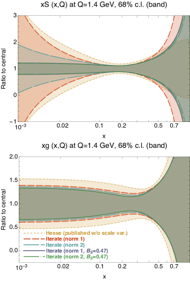
Figure 4: Ratios of the uncertainties to the respective central PDFs for the sea $xS(x,Q)$ (upper panel) and gluon $g(x,Q)$ (lower panel): xFitter published results [9] using Hesse evaluation of the uncertainties (without uncertainty from scale variations) in mustard; the same “norm 1” fit with Iterate uncertainties in medium-dashed red; and “norm 2” fit with Iterate uncertainties in long-dashed cyan. Then, for a fixed $B_{S}=0.47$, “norm 1” and “norm 2” fits are compared as overlapping dark blue and green curves.

Once the Fantômas environment has been set up using an independent C++ package, we have tested it against the published results of xFitter for the pion PDF [9]. For this initial comparison, we excluded the LN DIS data – a new component introduced in our fit.

When using the lowest-order polynomials ($N_{m}=0$), the parametrizations in Eqs. (2) and (15) differ only by their normalization, which we shall call “norm 1” and “norm 2.” In the case of xFitter parameterization “norm 1,” the normalizations $A_{V,S,g}$ directly determine the respective momentum fractions. The potential downside of the Euler beta function in the denominator of $xS(x,Q^{2}_{0})$ is that it introduces a nonlinear relation among $A_{S}$, $B_{S}$, and $C_{S}$ when calculating the uncertainty in the Hessian approach.

On the other hand, the parameters $A_{i}$ in the metamorph parametrization do not directly represent the momentum fraction of each flavor – that’s “norm 2.” To recover the results obtained with Eqs. (15), the metamorph degree is set to $N_{m}=0$, which requires one fixed control point for each PDF flavor $i$. With only the DY and prompt-photon data included, phenomenological separation of the sea and gluon distributions mainly relies on the choice of functional form and propagation on uncertainty into the extrapolation region, which in this specific case extends starting from $x\lesssim 0.1$ until the end point $x\sim 0$ for the whole $Q^{2}$ coverage. Hence, the small-$x$ behavior of the sea balances that of the gluon in a subtle way. The parameter $B_{S}$ that dominates the small-$x$ behavior of the sea is poorly determined, and even compatible with zero. We find that the propagation of the uncertainty following “norm 1” or “norm 2” does not render a similar result.

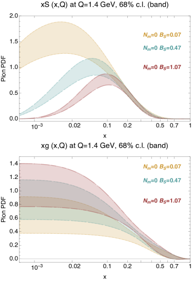
Figure 5: The Fantômas PDFs for $N_{m}=0$, based on DY+$\gamma$ data, shown for various values of the fixed parameter $B_{S}$. The upper panel (lower panel) shows the quark sea (the gluon) PDF and its uncertainty.

$N_{m}=0$ (DY+$\gamma$)	$\chi^{2}\,[d.o.f=379-5]$	$\langle xV\rangle$	$\langle xS\rangle$	$\langle xg\rangle$
$B_{S}=0.07$	$445.70$	$0.556$	$0.268$	$0.177$
$B_{S}=0.27$	$445.38$	$0.557$	$0.239$	$0.204$
$B_{S}=0.47$	$445.29$	$0.558$	$0.217$	$0.225$
$B_{S}=0.67$	$445.36$	$0.559$	$0.199$	$0.243$
$B_{S}=0.87$	$445.52$	$0.559$	$0.184$	$0.257$
$B_{S}=1.27$	$445.76$	$0.559$	$0.172$	$0.269$

Table 1: Momentum fractions for $N_{m}=0$ and DY+$\gamma$ data only. Correspond to fits shown in Fig. 5 at $Q^{2}=1.9$ GeV².

To explore the causes of such differences, we have considered two modalities for the Minuit diagonalization of the Hessian matrix in xFitter, namely Hesse and Iterate. The former is the default setting, while the latter comes from the CTEQ collaboration [71]. The 2020 xFitter study calculated the PDF uncertainties with the Hesse method. Figure 4 illustrates the differences between the outcomes of the two methods. While the best-fit PDFs agree, the Hesse error bands are larger than the Iterate ones. The instability in the Hessian diagonalization can be mended by fixing the small-$x$ power $B_{S}$ of the sea distribution. Thus, in Fig. 4 we compare error bands with a free $B_{S}$ and Hesse and Iterate methods with “norm 1” and “norm 2,” as well with a constant $B_{S}=0.47$ and Iterate with “norm 1” and “norm 2.” With $B_{S}$ fixed, both the Hesse and Iterate error bands agree much better for all three flavors and normalization types. Practically the same best-fit parameters and errors are found with all choices, as well $\chi^{2}/N_{\rm dof}=445.3/(379-5)=1.19$ at the best fit.

Poor determination of the small-$x$ behavior of the gluon with free $B_{S}$ leads to a confusion about the allowed values for the momentum fraction of the sea. The parameter $A_{S}$, quoted as $0.216\pm 0.025$ [9], translates into $A_{S}=6\pm 1$ for “norm 2” with fixed $B_{S}$ but delivers a much larger uncertainty, $A_{S}=6\pm 10$, when $B_{S}$ is free to vary.

After reproducing the nominal xFitter results using the new Fantômas module with $N_{m}=0$, a first extension naturally comes from varying the fixed value of the small-$x$ exponent of the sea distribution within some interval, which we take to be $B_{S}\in[0.07,1.07]$. The metamorph parameterizations are still used with $N_{m}=0$ for each flavor, i.e. the PDFs are given by their respective carrier functions in Eq. (1). In each of these fits, the valence PDF converges to the same function, whereas the sea and gluon PDFs change, with their magnitudes adjusting inversely to one another at $x<0.3$ as $B_{S}$ is varied [Fig. 5]. The corresponding momentum fractions are listed in Table 1. These results, combined with the $\chi^{2}$ results, indicate that the sea and gluon PDFs are not well constrained at low $x$. Analogous quantitative results for a DY-only analysis were reached by the JAM collaboration [8].

The individual fits for $B_{S}=\{0.07,\ 0.27$, $0.47,\ 0.67$, $0.87,\ 1.07\}$ also realize a Lagrange Multiplier scan over that parameter. The scan indicates a very shallow $\chi^{2}$ parabola (see the $\chi^{2}$ column of Table 1), which, in turn, indicates that the statistical loss from varying $B_{S}$ is negligible.

From this point on, we will develop the full Fantômas formalism within the xFitter fitting framework. By adding the LN DIS data at small $x$, we reduce, although not entirely eliminate, the small-$x$ degeneracy of the quark sea and gluon PDFs that was just discussed. This largely independent analysis with a different methodology will be compared again with the xFitter 2020 results in Sec. VI.

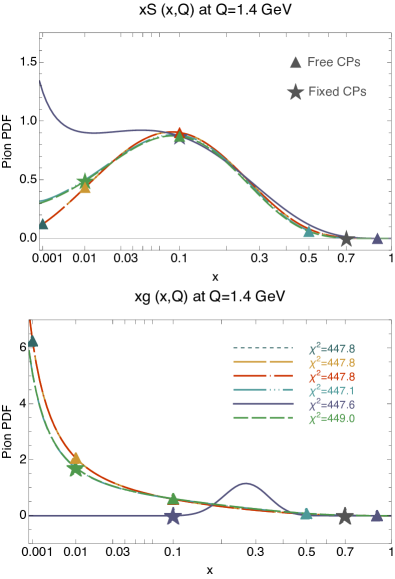
Figure 6: The sea and gluon pion PDFs obtained with the Fantômas environment for an $N_{m}=1$ and $\alpha_{x}=0.75$ setting, shown at $Q_{0}$. The control points are indicated for each curve with a star and a triangle for a fixed and free CP, respectively. Notice that all but two curves share a fixed CP at $x=0.7$.

IV The baseline Fantômas fit

Building upon a broader and more diverse data set illustrated in Fig. 3, we proceed with an in-depth investigation of functional form dependencies enabled by the Fantômas methodology. In the fits to the full data set, we start with $N_{m}=0$ parametrizations for all flavors $i{=}\{V,S,g\}$ and free carrier parameters. We then vary $N_{m}$ between 0 and 3 independently for each flavor by adding or removing free or fixed CPs. Recall that the number of CPs is kept equal to $N_{m}+1$, so that they uniquely determine the modulator polynomial. The shape of the best-fit PDF is controlled by the carrier parameters $A_{i},\ B_{i},\ C_{i}$, as well as by the degree $N_{m}$, stretching power $\alpha_{x}$, and placement of fixed CPs in the modulator. Positions of free CPs, on the other hand, do not modify the best-fit polynomial, given its uniqueness, and rather can be placed according to convenience (e.g., since the function values at CPs tabulate the PDF at user-chosen positions $x_{i}$). Altogether, the presented fits have at least 5 and at most 13 free parameters.

Figure 6 illustrates the variety of solutions obtained by selecting positions of the fixed and free CPs for $(N_{m}=1,\alpha_{x}=0.75)$. Using the same carrier and fixed CPs, but moving the abscissa of the free control point, we obtain very similar resulting sets with equally good $\chi^{2}$ values – see the first three labeled curves of Fig. 6. For other choices of the fixed control points, the gluon PDF differs in shape and can even get close to zero at $Q_{0}$, yet always staying non-negative. The latter solution also shows that the gluon has an additional freedom at $x\sim 0.3$, where experimental constraints are weak, as indicated by a bump in the fifth curve. The relative paucity of the pion data allows such solutions, as the Fantômas analysis reveals. The shown solutions have nearly the same $\chi^{2}$, all at least as good as the $\chi^{2}$ of the 2020 xFitter fit, cf. Table 1, despite having more data in the current study. The differences among the solutions in Fig. 6 enlarge the spread in the respective momentum fractions.

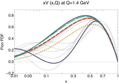
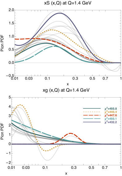
Figure 7: Central values for pion PDFs obtained with the Fantômas environment for various $N_{m}$, $\alpha_{x}$ and CP settings, shown at $Q_{0}=\sqrt{1.9}$ GeV. The baseline fits chosen for the final combination are shown in color. Light gray curves illustrate the many possible shapes that were obtained.

Expanding to higher degrees of the polynomial, whether across all or some flavors, revealed an even richer spectrum of potential solutions. Among these, the lowest $\chi^{2}$ value observed in our limited sample was $414$, corresponding to a negative sea distribution at large-$x$ values. Figure 7 presents a subset of about $\sim 100$ such configurations. In color, we display the fits that are kept for the final combination, for which the fit with the lowest chi-square value ($\chi^{2}=432.2$) corresponds to a zero-gluon distribution. The second-best $\chi^{2}=440.4$ belongs to a configuration that exhibits a negative gluon PDF around $x\simeq 0.1$. The expected variance of the chi-square for $N_{\rm pts}=408$ and varying $N_{\rm par}$ between 7 and 13 amounts to $\delta\chi^{2}=\sqrt{2(N_{\rm pts}-N_{\rm par})}\simeq 30$ at the $1\sigma$ level [7]. We retain fits with $\chi^{2}\lesssim 450$, a few units below the variance of $\chi^{2}_{\rm min}=432$. Most of the metamorph sets exhibit chi-square values well within $1\sigma$ from the minimum value that was obtained.

The spread of the solutions in Fig. 7 quantifies the parametrization dependence that contributes to the epistemic uncertainty. As we reminded in Sec. II.3 using a toy example, the epistemic uncertainty (corresponding to the lower panel in Fig. 2) is independent from the aleatory one. The latter could be either estimated by resampling/bootstrapping the data $N_{\rm rep}$ times, as illustrated in the upper panel of Fig. 2 and followed by JAM, or alternatively by diagonalization of the Hessian matrix [73], as done in xFitter. The 68% c.l. aleatory uncertainties quoted by xFitter correspond to a variation of $\Delta\chi^{2}=1$ around the minimum of a single fit, which has long been known to lead to error bands that are excessively narrow. To these, we should add the epistemic uncertainty, the core rationale behind our investigation.

In many practical applications with parsimonious parametric dependence, a useful estimate of epistemic uncertainties may be possible through sufficiently representative sampling of acceptable PDF models [33]. We follow this paradigm by first generating uncertainty bands with $\Delta\chi^{2}=1$ from several parametrizations with good $\chi^{2}$ and a broad span in the PDF magnitudes; Fig. 7 shows the central PDFs for five such selected parametrizations in color. We then generate a combined PDF error set from these error bands using the METAPDF method [40]. This combination technique is more direct than introducing either the global or dynamic tolerance, while operationally it serves the same purpose of accounting for the parametrization uncertainty as done, e.g., by introducing the tolerance $\Delta\chi^{2}>1$ in the CTEQ-TEA analyses [32]. In extrapolation regions with no data or first-principle constraints, the PDF combination techniques avoid unrealistically small uncertainty that are common with the customary tolerance prescriptions. Tensions among the fitted data sets – the other rationale for increasing the tolerance in global fits [7, 73, 74] – are not relevant in this pion fit.

Selection of the PDF solutions unavoidably depends on the prior constraints, such as smoothness of PDFs and positivity of cross sections. In this study, smoothness is achieved by using polynomials with low $N_{m}$ and sufficient spacing of control points to suppress the Runge phenomenon (cf. Sec. II.5). Notably, the pion data do not disfavor and even prefer the quark and sea gluon PDFs that go negative in certain $x$ intervals at the initial scale $Q_{0}^{2}=1.9\mbox{ GeV}^{2}$ or have local extrema. For example, this feature applies to the negative gluon shown by a short-dashed mustard curve in Fig. 7. JAM collaboration has also found such solutions [10]. We, however, choose to discard strongly negative PDFs, some of which are displayed in light gray. We include some solutions with weakly negative PDFs to capture the enhanced uncertainty in the gluon and sea sectors at $(x\simeq 0.1,Q\gtrsim Q_{0})$ and in other extrapolation regions that must be further constrained by future data.

The positivity of distribution functions, as a first-principle argument, has been a topic of various research publications [75, 76, 77]. Hadron-level cross sections must be non-negative everywhere in $x$ and $Q^{2}$. Whether this necessitates non-negative PDFs in perturbative QCD depends on other factors, including the order and scheme of the calculation, mixing of scattering channels, all-order resummations and a variety of nonperturbative contributions [see a general discussion in Ref. [48] and Ref. [78, 11] for threshold resummation]. Furthermore, QCD evolution turns mildly negative PDFs at $Q_{0}$ and small $x$ into positive ones at slightly higher $Q$ values where perturbative QCD dominates. Requiring the PDFs to be non-negative at small $Q_{0}$, where perturbative QCD ceases to converge, may artificially suppress the PDF uncertainty at larger $Q$, where the positivity is no longer an issue. In fact, the issue of positivity could be entirely avoided for such PDFs by choosing a slightly higher $Q_{0}$ to start with, at the expense of a slightly higher $\chi^{2}$ – we have checked that it is the case for the sets that display a negative gluon at $x\to 1$. Dependence of pion PDFs on $Q_{0}$ must be explored in further studies, as it is known to be relevant since the early model evaluations both for the PDFs and exclusive form factors, e.g. in  [29, 30].

To recap, the five fits that constitute the final FantoPDF ensemble are highlighted with bold colors and fonts on Fig. 7. They are chosen for their distinct shapes, thereby maximally spanning the parameter space explored across the $\sim 100$ metamorph configurations that have been tested. Among these selected outcomes, the dashed-mustard curve corresponds to a metamorph configuration yielding a slightly negative gluon distribution in the $x\simeq 0.1$ extrapolation region. These fits are combined using the METAPDF technique that captures the bulk of the explored parametrization uncertainty, even though it does not include some extreme baseline solutions with negative PDFs, with some shown in grey in Fig. 7.

V The Fantômas parton distributions of the pion

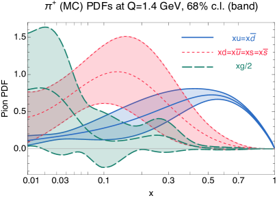
Figure 8: The FantoPDF sets at $Q_{0}$, shown for a $\pi^{+}$ flavor configuration.

Figure 8 displays the combined Fantômas pion PDF ensemble, constructed from the five fits for which the chi-square values of the central PDF range between $\chi^{2}/N_{\rm pts}$ of 1.06 (432/408) and 1.10 (450/408), improving upon the xFitter’s original DY+$\gamma$ fit quality. The error bands of the combined ensemble are determined with the METAPDF package [40] by first generating 100 Monte-Carlo replicas from each of the five input ensembles, and then combining the replicas into the final Fantômas Monte-Carlo ensemble. The combination proceeds using symmetric uncertainties, linear scaling, as well as a small shift of the final central PDFs so that they are equal to the averages of the corresponding central PDFs of the input ensembles [54]. The original ensembles are not weighted, as the differences in their numbers of degrees of freedom are negligible with respect to the number of data points $N_{\rm pts}$. This procedure is analogous to the PDF4LHC21 combination [80].

Figure 9: Momentum fractions for the sea and gluon PDFs obtained in the five baseline fits (orange-brown) and the MC FantoPDF combination (green ellipse) at $Q_{0}$. JAM21 and xFitter results are displayed in red and blue, respectively.

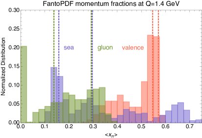
Figure 10: The histograms represent momentum fractions for the valence (red), gluon (green) and sea (blue) PDFs from 500 MC FantoPDF distributions generated from five candidate fits. The histograms are not symmetric as a consequence of parametrization dependence. Vertical boundaries represent the extrema of momentum fractions for pre-Fantômas fits with DY+$\gamma$ data only (Fig. 5). These results are at the initial scale $Q_{0}$.

The statistical meaning of the Fantômas ensemble differs from the one expected from resampling (importance sampling), as it it covers both types of uncertainties (aleatory and epistemic) illustrated in the two panels of Fig. 2. The aleatory uncertainties are estimated by the Hessian error bands for the unfluctuated (published) data for each of the five PDF fits that sample the epistemic uncertainty. To apprehend the latter, the sampling of the PDF models should be sufficiently dense in multidimensional space of parameters, as discussed in [33] and references therein. While sampling becomes a daunting problem in space of many dimensions, its efficiency can be drastically improved in specific applications by optimizing a quantity called a confounding correlation or data defect correlation [81, 82]. Thus, the five fits reasonably capture the spread of PDFs from about a hundred candidate fits obtained in the first step of our study. The likely distances between the true PDFs and their fitted parametrizations are thus determined by the interplay of the confounding correlations with the data quantity and aleatory uncertainties of the data itself.

From this ensemble of pion PDFs with comparable $\chi^{2}$, we can compute the momentum fractions $\langle xf\rangle$ integrated over the whole range of $x$. The valence sum rule governs the momentum fraction for $V(x,Q_{0})$, while the momentum sum rule relates the sea and gluon momentum fractions. Figure 9 illustrates the latter at scale $Q_{0}$, with variations in $\langle xS\rangle$ showing a strong correlation with $\langle xg\rangle$. Here, we plot the momentum fractions for the five baseline fits as well as for the final FantoPDF combination. We also superimpose the respective momentum fractions from JAM’21 [11] and xFitter [9] analyses – they will be discussed in detail in the next section.

The picture that emerges is that the flexibility of the functional form strongly affects conclusions about the experimentally allowed momentum fractions by increasing their ranges compared to the fits with fixed parametrization forms. We can further illustrate this point by examining the histograms in Fig. 10 for momentum fractions for $\braket{xV}$, $\braket{xS}$, and $\braket{xg}$ obtained with 500 replicas from the five baseline sets. The parametrization dependence in the DY+$\gamma$+LN fit substantially widens the histograms as compared to the full intervals (vertical dashed lines) from the DY+$\gamma$ fit with the fixed functional form in Sec. III.3. In particular, the addition of leading-neutron data only partially improves the separation between sea and gluon distributions compared to the pre-Fantômas analysis of the DY-only data [Fig. 5]. Addition of the LN data is not by itself sufficient for narrowing the interval of the allowed sea and gluon momentum fractions. The long $\braket{xS}$-$\braket{xg}$ correlation ellipse for the final Fantômas combination in Fig. 9 supports this assessment, which is somewhat in a contradiction with the JAM analyses [8] – see Sec. VI.

Figure 11: The effective $(1-x)$ exponent of the valence PDF in the FantoPDF ensemble – the definition is given in [48]. In green, the effective exponent at $Q_{0}=\sqrt{1.9}$ GeV and, in blue, at $\sqrt{10}$ GeV. The plot is cut at $x=0.94$ for grid-extrapolation reasons. We have verified analytically that the highlighted Bézier curves of Fig. 7 converge to $C_{V}^{\mbox{\tiny eff}}=1$ at most for $x\to 1$ at $Q_{0}$.

While we allow marginally negative fits, the final results produce positive momentum fractions for all components at $Q_{0}$. Table 2 (upper row) summarizes the results for the momentum fractions at $Q_{0}$. The $q+\bar{q}$ and gluon momentum fractions are given at $Q=2$ GeV in Table 3 (upper row).

We conclude this section by reviewing our findings for the pion valence PDF in the limit $x\to 1$. Recent debates on manifestations of nonperturbative dynamics in high-energy data made the large-$x$ behavior of the pion quark PDF a go-to topic [4, 41, 1, 11]. The quark-counting rules – an early prediction reflecting the kinematic constraints in the quasielastic region – suggest a $(1-x)^{\beta=2}$ fall-off of the pion quark PDFs when $x\to 1$. This expectation does not account for many dynamic contributions at either low or large momentum fractions that affect interpretation of realistic measurements [48]. In this regard, the present phenomenological analysis does not qualitatively differ from the previous recent ones: the fall-off of the valence PDF at large $x$ is compatible with $\beta=C_{V}^{\mbox{\tiny eff}}=1$ at $Q_{0}=\sqrt{1.9}$ GeV (see Fig. 11), in spite of the multiple functional forms that have been considered (Fig. 7).

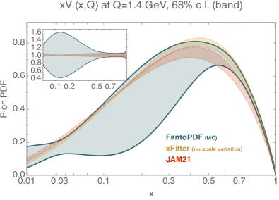
Figure 12: The valence PDF of the final Fantômas ensemble compared to JAM21 and xFitter results, at $Q=1.4$ GeV. For the FantoPDF set, the $68\%$ CL of the MC output is shown. xFitter’s results are plotted without accounting for the uncertainty coming from the scale variation. The inner frame shows the ratio to the central value of each set – symmetric uncertainties are used for all three sets.

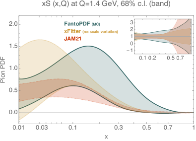
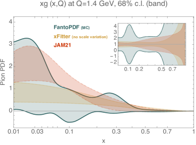
Figure 13: Same as in Fig. 12, for the quark sea PDF (top), gluon PDF (bottom).

VI Comparison with other global analyses

Now that we have established the power of the metamorph parametrization in the Fantômas formalism, we proceed to further comparisons of our results to previous extractions of the pion PDFs at NLO. The fitted data sets vary among the fitting groups. While the Fantômas analysis augments the full DY and prompt photon data set of xFitter with $29$ LN DIS data points, JAM authors choose to fit DY data only for invariant masses lower than the $\Upsilon$ mass (noticeable around $\mu^{2}=100$ GeV² in Fig. 3) and a larger pool of LN DIS data. The latter choice of data stems in turn from a combined study of the E866 proton $\bar{d}-\bar{u}$ and the HERA (H1 and ZEUS) LN DIS in the context of a pion-cloud approximation [65]. Our analyses differ hence in the precision with which the LN data are treated.

JAM’18 [8] reports a best fit of $\chi^{2}/N_{\rm pts}{=}0.98\ (244.8/250)$, with this number being obtained with a specific prescription for the pion flux in Eq. (LABEL:eq:pionSF). JAM’21 [11] adds large-$x$ resummation corrections in cross sections for the DY data; however, their baseline fit achieves $\chi^{2}/N_{\rm pts}=0.81$. The double Mellin method for the resummation marginally improves this result, while other resummation methods worsen it. JAM’s low $\chi^{2}$ value might result from the specific selection of cuts and models for the data. [The objective of the Fantômas analysis was not to explore the model dependence within the LN data]. On the other hand, the xFitter pion fit has achieved $\chi^{2}/N_{\rm pts}=1.17\ (444/379)$, or 1.19 with respect to the number of degrees of freedom quoted in [9].

Turning our attention to the shape of the distributions, we observe that, for the valence sector, the Fantômas PDF is in a good overall agreement with both JAM’21 and xFitter’s results, while displaying a larger uncertainty in the mid- and especially small-$x$ regions (Fig. 12). The existing DY data do not provide sufficient separation between the quark and antiquark PDFs at $x<0.2$, which spectacularly increases the uncertainty on $V(x,Q_{0})$ at small $x$ compared to the fixed-parametrization fits (in fact, allowing $V(x,Q_{0})$ to go negative in some baseline fits, cf. the upper panel of Fig. 7). The $x\to 1$ limit of the Fantômas ensemble is slightly narrower than for JAM’21, possibly because the Fantômas’s result was obtained by fitting the unfluctuated data, as opposed to the bootstrapped one by JAM.

The JAM and xFitter error bands in Fig. 12 demonstrate another common artifact of fixed polynomial forms – a pinch point at $x\approx 0.15$, where the uncertainty of $xV(x,Q)$ spuriously vanishes. A pinch point may emerge at some point due to a too restrictive parametric model. The pinch point disappears in the Fantômas error band, which combines multiple parametric forms.

The sea and gluon PDFs go hand-in-hand, as they are tied by DGLAP evolution as well as by the momentum sum rule constraint. The sea FantoPDF (Fig. 13, upper panel) exhibits an extremum around $x=0.15$ for $Q=Q_{0}$ that is not fully covered by either JAM or xFitter uncertainties. The Fantômas uncertainty increases towards smaller values of $x$, encompassing JAM’21. [The xFitter’s uncertainty for the sea is larger at $x>0.5$ as a consequence of their different Hessian diagonalization routine, as discussed in Section III.1.] The Fantômas gluon is enlarged across the whole span of $x$. The inner frames of Figs. 12 $\&$ 13 show the ratios to the central PDF of the corresponding sets. The mid-$x$ range might be sensitive to the choice of the model for the pion flux in the description of the LN data. Also, it corresponds to the transition from the LN and the pion-induced DY data set, while still being bridged by the prompt-photon data. The Fantômas fit is the first to include all three processes, on top of the Fantômas framework that accounts for uncertainty sources beyond the aleatory one.

Name	$Q$ [GeV]	$\langle xV\rangle$	$\langle xS\rangle$	$\langle xg\rangle$
FantoPDF (DY+$\gamma$+LN)	$\sqrt{1.9}$	$0.49(8)$	$0.34(19)$	$0.18(12)$
xFitter [9] (DY+$\gamma$)	$\sqrt{1.9}$	$0.55(6)$	$0.26(15)$	$0.19(16)$
xFitter w/o scale variation	$\sqrt{1.9}$	$0.55(2)$	$0.26(9)$	$0.19(9)$
JAM’18 [8] (DY)	$1.27$	$0.60(1)$	$0.30(5)$	$0.10(5)$
JAM’18 [8] (DY+LN)	$1.27$	$0.54(1)$	$0.16(2)$	$0.30(2)$
JAM’21 [11] (DY+LN)	$1.27$	$0.53(2)$	$0.14(4)$	$0.34(6)$
JAM’21 [11] (DY+LN)
+NNL double Mellin	$1.27$	$0.46(3)$	$0.15(7)$	$0.40(5)$
CT18 NLO (proton)	$\sqrt{1.9}$	$0.443(6)$	$0.160(10)$	$0.396(10)$
CT18 NNLO (proton)	$\sqrt{1.9}$	$0.451(5)$	$0.157(10)$	$0.390(10)$

Table 2: Pion (rounded) momentum fractions from global analyses (including this work) at $68\%$ C.L., at $Q_{0}=\sqrt{1.9}$ GeV for the xFitter-based frameworks and $Q_{0}=1.27$ GeV for JAM. The FantoPDF results quote the MC central values and symmetric errors. The 7th and 8th rows quote JAM’21 results with, respectively, the baseline and their preferred large-$x$ resummation technique. The last two rows quote the momentum fractions for the equivalent PDF flavors in the proton from CT18 fits [32].

The first two global analyses of the pion data were performed by the SMRS [12] and GRV [14] groups in the early 90s. At that time, the trend given by the NA3 data on pion-induced Drell-Yan [83] was that the gluon contribution to the momentum fraction was about $47\%$ at $Q^{2}=4$ GeV². This fraction was used as a baseline to improve the determination of the sea PDF, resulting in a very small sea contribution. SMRS used a simple $(1-x)^{\beta}$ ansatz for both the sea and the gluon and explored the space of allowed momentum fractions for the sea starting from $5$ to $20\%$, while keeping fixed $(\beta_{S},\beta_{g})$ parameters. They found that a sea momentum fraction as low as $5\%$ badly fits the NA10 data, and that the $\chi^{2}$ improves when the sea fraction is increased. On the other hand, GRV adopted a no-sea and valence-like gluon at the initial scale. This scenario similarly leads to a small momentum fraction for the sea, but no further study on the dependence on the model or scans on momentum fraction was done. Both studies were performed at NLO. The values of $\alpha_{s}(Q^{2})$ at that time were given in term of $\Lambda_{\mbox{\tiny QCD}}$ – a comparison to the modern use of $\alpha_{s}(M_{Z}^{2})$ might lead to increased differences.

Following upon these early works, in Table 2 we collect the pion momentum fractions from the recent phenomenological fits. As was already alluded in Sec. V in connection with Fig. 9, both xFitter and FantoPDF fits prefer a larger $\braket{xS}$ and smaller $\braket{xg}$ as compared to JAM, which primarily reflects the preference of the NA10 data (JAM21 uses a set of 56 NA10 data) for a higher quark sea. The scenario in which the gluon carries above 40% of the momentum is disfavored on these grounds, as it results in a too low (anti)quark sea that undershoots the experimental DY cross sections. On the other hand, solutions with a low or even zero gluon improve the description of the DY data and produce low $\chi^{2}$ values. This conclusion may depend on the order of perturbative QCD calculation and the choice of nuclear PDFs, the factors that will need to be further explored.

The Fantômas uncertainties quoted in Table 2 are significantly larger than from the other groups’ fits, reflecting our addition of the parametrization dependence. Upon inclusion of the LN DIS data in the Fantômas analysis, the ordering of the $\braket{xS}$ and $\braket{xg}$ magnitudes remains the same within the uncertainties. This can be contrasted with the JAM’18 [8] results in rows 4 and 5 of Table 2, where the ordering of $\braket{xS}=0.30\pm 0.05$ and $\braket{xg}=0.10\pm 0.05$ changed to $\braket{xS}=0.16\pm 0.02$ and $\braket{xg}=0.30\pm 0.02$ after adding the LN data to the fit. For the gluon momentum fraction, our estimate for the experimentally allowed interval is $0\leq\braket{xg}\leq 35\%$ at the $2\sigma$ level at $Q_{0}=\sqrt{1.9}$ GeV. For the quark sea, it is $12\leq\braket{xS}\leq 69\%$, in consistency with the MC histograms in Fig. 10.

VII Comparison with lattice evaluations

Lattice QCD evaluations are playing an increasingly important role in determining distribution functions from first principles. The field is flourishing with the advent of large-momentum effective theory (LaMET) for lattice evaluations [84, 85], followed by alike formalisms such as Ioffe-time distributions (leading to pseudo-PDFs) [86, 87, 88].

Several lattice methodologies are available for determination of the components of pion PDFs [89, 90]. The first one consists in a computation of the Mellin moments of PDFs. Advanced methods include fits of discrete lattice predictions for bare matrix elements of the pion, as well as the quasi-PDF approach of LaMET. The quasi-PDF can be related to the $P_{z}$-independent light-cone PDF through a factorization theorem that identifies a perturbative matching coefficient with corrections suppressed by the hadron momentum. Various groups have evaluated pseudo- or quasi-PDFs to NLO [17, 18, 19, 20, 21, 22, 24] and well as to NNLO [25, 26] using perturbative matching between the Euclidean time quantities and the light-cone PDF. Predictions for the gluon PDF in the pion and its momentum fraction are available in Refs. [91, 23, 92].

Name	$Q$[GeV]	$\langle x(u+\bar{u})_{\pi^{+}}\rangle$	$\langle xg\rangle$
FantoPDF	$2$	$0.331(25)$	$0.24(10)$
HadStruct [19]	$2$	$0.2541(33)$	–
Ref. [20]	$3.2$	$0.216(19)(8)$	–
ETM [46]	$2$	$0.261(3)(6)$	–
Ref. [93]	$2$	–	$0.37(8)(12)$
Ref. [91]	$2$	–	$0.61(9)$
Ref. [92]	$2$	–	$0.364(38)(36)$
ZeRo Coll. [94]	$2$	$0.245(15)$	–
Ref. [95]	$7$	$0.02$	–

Table 3: Momentum fractions from the FantoPDF global analysis, PDF-oriented lattice analyses, and early lattice evaluations. Lattice collaborations give the combination $u_{+}=v/2+2\bar{u}$ for the $\pi^{+}$ for even (“odd” in lattice nomenclature) moments. Lattice uncertainties are quoted as “statistical” and “systematic,” respectively.

In the pion sector, the lattice data become predictive enough to complement the experimental data that are still mainly based on the pion-induced DY process. Lattice predictions may even circumvent the complex theoretical aspects that arise in phenomenological fits when the pion PDF is determined in perturbative QCD at a relatively low scale $Q_{0}$ [48]. The current lattice predictions for PDFs are most trusted at $0.2\lesssim x\lesssim 0.8$, although their extension to even larger $x$ can be informative given some contention about the behavior of the pion PDFs in the $x\to 1$ limit. For the valence PDF, lattice groups have found the effective large-$x$ exponent [53, 48] in the range $0.5\lesssim\beta[=C_{V}^{\mbox{\tiny eff}}]\lesssim 2$ at a low scale, showing a strong dependence on the choice of methodology by each lattice group, including handling of the inverse problem and fits, as discussed in [20, 96]. The NNLO results of Ref. [25] show compatibility of several lattice representations of the pion PDF with $\beta[=C_{V}^{\mbox{\tiny eff}}]=1$. As discussed in Sec. V, our analysis is in agreement with the previous fixed-order extractions [8, 9] as well as those lattice determinations that obtain $\beta=1$. Notice, however, that the uncertainty at mid-$x$ values is larger on those lattice results, as a result of the corresponding fitting procedure and the lack of accuracy towards smaller $x$ values. In particular, the Fantômas valence PDF, with its wider uncertainty for the valence region (Fig. 7), is compatible with the NNLO lattice pion PDF [25], as illustrated in Fig. 14.

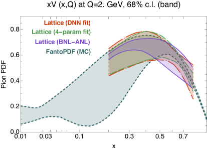
Figure 14: Valence pion PDF $xV(x,2$ GeV$)$ for the FantoPDF in dark cyan, as well as for the lattice result of [25] in red (DNN version) and green (4-parameter version), and BNL-ANL21 [97] in purple.

Recently, Ref. [98] put forth a hybrid determination using both raw lattice data for reduced Ioffe time pseudo-distributions and current-current correlator, as well as experimental data. Results were found for the valence PDF, and no significant increase in $C_{V}^{\mbox{\tiny eff}}$ is reported.

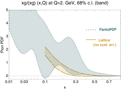
Figure 15: Gluon pion PDF normalized to its momentum fraction $xg(x,2$ GeV$)/\langle xg(x,2$ GeV$)\rangle$ for the FantoPDF in dark cyan and for the lattice result of [23] in yellow mustard. Only statistical uncertainties are quoted for the lattice prediction.

The lattice estimate of the gluon PDF [23] shows a large dependence on the choice of functional form for $x<0.5$, where the lattice extrapolation region starts. Fantômas results are compatible with that lattice evaluation at large $x$ [see Fig. 15], though we cannot conclude on the true uncertainty of the lattice determination. The lattice-predicted PDF is normalized to its momentum fraction, leaving the determination of the overall moment aside, and does not include potentially significant systematic uncertainties. That analysis has been recently complemented by evaluating the gluon momentum fraction [92]. The authors state that the resulting, absolute, gluon PDF is in agreement with previous global analyses.

In Table 3, we also compare our results for the second moments of the Fantômas pion PDF with some lattice results for the $q_{+}$ combination. On the lattice, one can compute odd moments (corresponding to even powers of $x$ in the integrand) for the “minus” non-singlet distributions, $q-\bar{q}$, and even moments (corresponding to odd powers) for the “plus” distributions. Due to its large sea component, the Fantômas ensemble’s second-Mellin moment overshoots the current lattice estimations. In the fourth column, we compare the momentum fraction of the Fantômas PDF for the gluon with some lattice estimates. Notably, the gluon PDF cannot be estimated simultaneously with the valence distribution on the lattice. The quoted momentum fractions, obtained for values $m_{\pi}^{\rm latt}\gg m_{\pi}^{\rm phys}$, are rather large. The momentum fraction $\braket{xg}=0.61\pm 0.09$ obtained from the analysis of the gravitational form factor [91] leaves very little room for the momenta of the valence and sea distributions. In that sense, it is hardly compatible with the state-of-the-art valence momentum fractions on the lattice, nor with the Fantômas output, despite the large uncertainty of the latter.

Regarding the reconstruction of the $x$-dependence of the pion valence PDF from lattice moments, we evaluate the odd moments for $u^{\pi^{+}}$ and compare to the results obtained in Ref. [25], see Table 4. The third and fifth moments are in good agreement, while the seventh is higher for the FantoPDF set [similar results are obtained in JAM21, see Fig. 10 of [25]]. The behavior of the valence quarks from the Fantômas methodology agrees with lattice determinations up to high moments.

Name	$\langle x^{2}u^{\pi^{+}}\rangle$	$\langle x^{4}u^{\pi^{+}}\rangle$	$\langle x^{6}u^{\pi^{+}}\rangle$
FantoPDF	$0.117(5)$	$0.042(1)$	$0.021(1)$
Ref. [25]	$0.1104(73)(48)$	$0.0388(46)(57)$	$0.0118(48)(48)$

Table 4: Odd Mellin moments compared to the lattice evaluation of Ref. [25], at 2 GeV.

VIII Conclusions

In this study, we extend the informative phenomenological NLO analysis [9] of charged pion PDFs implemented in the xFitter program to include the PDF parametrization dependence – an important factor in the total uncertainty on PDFs that was not considered by previous pion studies. The magnitude of uncertainty tolerated by experimental measurements affects comparisons with predictions for PDFs by nonperturbative QCD approaches. Reliable quantification of uncertainties becomes pivotal in light of the encouraging new developments both in theoretical simulations and experimental measurements of the meson structure.

The essence of the phenomenological global analyses consists in finding a range of functional forms for the PDFs that are compatible with the experimental data. Any such parton distribution can be approximated by polynomials in the momentum fraction $x$ at a low scale $Q_{0}$ as a consequence of the Stone-Weierstrass theorem. Hence, evidence for PDFs translates into a certain functional, and even often polynomial, behavior. As argued in Ref. [48], the property of polynomial mimicry hinders a unique “if and only if” discrimination among the functional behaviors. Mimicry implies the equivalence in describing the same discrete data by multiple polynomial shapes of (often) differing orders in interpolations. In global analyses for which an initial assumption about the allowed functional forms is necessary, the choice of a polynomial shape contributes to the epistemic uncertainty of the final PDF ensemble. This uncertainty plays an increasing role with growing precision of measurements  [7, 32, 33] and must reflect generic prior considerations such as positivity [75, 76, 77] or flavor structure in asymptotic limits [32, 99].

Interestingly, the uncertainty quantification in the context of polynomial shapes is also of concern to any analysis facing an inverse problem; it has been discussed for lattice determinations of, e.g., the shape of the valence pion PDF [20, 96]. Nonparametric methodologies for QCD global analyses, such as those based on ML/AI, are not free from that source of uncertainty. One way to address the epistemic uncertainty is to estimate it by representative sampling of acceptable functional forms [33]. The open-ended inverse problem of finding the epistemic uncertainty is also ill-posed, yet sufficiently dense sampling over the functional forms provides at least a lower estimate with well-designed, parsimonious parametric models.

In this manuscript, we explore the positive aspect of the polynomial mimicry. In Ref. [48], we contemplated the possibility of using Bézier curves – linear combinations of Bernstein polynomials of a user-specified polynomial degree – as continuous approximations of PDFs determined by the PDF values at a few chosen points in $x$. The algorithmic nature of such construction makes it versatile yet more transparent than the complementary approaches based on neural networks. Indeed, a Bézier parametrization is directly defined by the PDF values at control points and not by latent parameters and hyperparameters of a neural network. We introduced Fantômas, a C++ program providing metamorph parametrizations for PDFs that capture the asymptotic limits at $x\to 0$ and $x\to 1$ using the carrier component and any features of PDFs at intermediate $x$ using the modulator component. The modulator function includes a Bézier curve of degree $N_{m}$ with coefficients determined by $N_{m}+1$ control points that are optimally placed according to the problem to solve. When solving the inverse problem for PDFs, minimization of the objective function varies the free parameters of the carrier function and values of the modulator at the control points. A variety of functional forms can be generated on the fly by using different carriers, placements of fixed control points, and the $x$-stretching variable in the modulator.

This metamorph parametrization module has been implemented into the xFitter QCD fitting framework and tested in the pion analysis at NLO that has been already implemented in  [9]. The latter analysis complements the panorama offered by the three JAM fits (collinear [8], with the inclusion of large-$x$ resummation [11], and simultaneous collinear and TMD fitting [10]) and expands on the pioneering QCD analyses of the pion PDFs in [12, 13, 14]. The xFitter analysis uses the Hessian methodology [73, 74] to estimate aleatory uncertainties associated with the data. To the aleatory uncertainties, we add the epistemic ones obtained by systematic sampling of about 100 modulator forms with degree up to $N_{m}=3$. We find that the range of pion PDFs rendering essentially the same $\chi^{2}$ is significantly increased by considering multiple functional forms.

The most constraining set of the experimental data, coming from the pion-induced Drell-Yan pair production on a tungsten target, is characterized by large momentum fractions for the pion beam. Even after inclusion of the leading-neutron DIS data constraining the gluon PDF down to $x\sim 10^{-3}$, the available experimental measurements only weakly separate the quark and antiquark PDFs, and the quark sea and gluon PDFs at $x<0.2$. The consequence is the enlarged uncertainty bands in the Fantômas PDF ensemble seen in Figs. 12 and 13, as well as the extended range of the correlated momentum fractions for the quark sea and gluon in Fig. 9. The Fantômas analysis finds that $\braket{xg}$ in the range from 0 to 35% are allowed by the data. This is a wider range than what was found with fixed parametrization forms.

A curious tension therefore emerges between the small momentum fractions $\braket{xg}$ that may in fact be preferred by the NA10 DY data (which is more extensive in xFitter than in the JAM analysis), and the first lattice QCD predictions suggesting $\braket{xg}$ above 30%, as summarized in Table 3. These observations raise the value of the ongoing and planned pion scattering experiments at AMBER [42] and EIC [4, 41]. The dependence of DY constraints on the assumed nuclear PDFs needs to be further explored, and additionally, this and other [9, 8, 11] phenomenological studies are still dominated by the low-$Q$ data for which higher-order perturbative QCD uncertainties need to be reduced. We did not add the uncertainty due to the QCD scale variations – its magnitude can be gauged from the comparison of the xFitter momentum fractions with and without the scale-variation uncertainty in Table 2. Besides the PDFs, description of some pion observables by the nonperturbative theoretical techniques and transition to the perturbative regime is still insufficiently understood [29, 30, 100]. The pion structure will thus remain an exemplar to develop QCD methods. Our xFitter analysis will be made publicly available together with the Fantômas module and LHAPDF grids for the NLO pion error PDFs that we produced.

References

- [1] R. Abdul Khalek et al., “Science Requirements and Detector Concepts for the Electron-Ion Collider: EIC Yellow Report,” Nucl. Phys. A 1026 (2022) 122447, arXiv:2103.05419 [physics.ins-det].
- [2] AMBER Collaboration, C. Quintans, “The New AMBER Experiment at the CERN SPS,” Few Body Syst. 63 no. 4, (2022) 72.
- [3] A. Accardi et al., “Strong Interaction Physics at the Luminosity Frontier with 22 GeV Electrons at Jefferson Lab,” arXiv:2306.09360 [nucl-ex].
- [4] A. C. Aguilar et al., “Pion and Kaon Structure at the Electron-Ion Collider,” Eur. Phys. J. A 55 no. 10, (2019) 190, arXiv:1907.08218 [nucl-ex].
- [5] X. Ji, Y.-S. Liu, Y. Liu, J.-H. Zhang, and Y. Zhao, “Large-momentum effective theory,” Rev. Mod. Phys. 93 no. 3, (2021) 035005, arXiv:2004.03543 [hep-ph].
- [6] R. Abir et al., “The case for an EIC Theory Alliance: Theoretical Challenges of the EIC,” arXiv:2305.14572 [hep-ph].
- [7] K. Kovařík, P. M. Nadolsky, and D. E. Soper, “Hadronic structure in high-energy collisions,” Rev. Mod. Phys. 92 no. 4, (2020) 045003, arXiv:1905.06957 [hep-ph].
- [8] P. C. Barry, N. Sato, W. Melnitchouk, and C.-R. Ji, “First Monte Carlo Global QCD Analysis of Pion Parton Distributions,” Phys. Rev. Lett. 121 no. 15, (2018) 152001, arXiv:1804.01965 [hep-ph].
- [9] I. Novikov et al., “Parton Distribution Functions of the Charged Pion Within The xFitter Framework,” Phys. Rev. D 102 no. 1, (2020) 014040, arXiv:2002.02902 [hep-ph].
- [10] Jefferson Lab Angular Momentum Collaboration, N. Y. Cao, P. C. Barry, N. Sato, and W. Melnitchouk, “Towards the three-dimensional parton structure of the pion: Integrating transverse momentum data into global QCD analysis,” Phys. Rev. D 103 no. 11, (2021) 114014, arXiv:2103.02159 [hep-ph].
- [11] Jefferson Lab Angular Momentum (JAM) Collaboration, P. C. Barry, C.-R. Ji, N. Sato, and W. Melnitchouk, “Global QCD Analysis of Pion Parton Distributions with Threshold Resummation,” Phys. Rev. Lett. 127 no. 23, (2021) 232001, arXiv:2108.05822 [hep-ph].
- [12] P. J. Sutton, A. D. Martin, R. G. Roberts, and W. J. Stirling, “Parton distributions for the pion extracted from Drell-Yan and prompt photon experiments,” Phys. Rev. D 45 (1992) 2349–2359.
- [13] M. Gluck, E. Reya, and A. Vogt, “Pionic parton distributions,” Z. Phys. C 53 (1992) 651–656.
- [14] M. Gluck, E. Reya, and I. Schienbein, “Pionic parton distributions revisited,” Eur. Phys. J. C 10 (1999) 313–317, arXiv:hep-ph/9903288.
- [15] C. Bourrely, W.-C. Chang, and J.-C. Peng, “Pion Partonic Distributions in the Statistical Model from Pion-induced Drell-Yan and Production Data,” Phys. Rev. D 105 no. 7, (2022) 076018, arXiv:2202.12547 [hep-ph].
- [16] MAP Collaboration, B. Pasquini, S. Rodini, and S. Venturini, “The valence quark, sea, and gluon content of the pion from the parton distribution functions and the electromagnetic form factor,” arXiv:2303.01789 [hep-ph].
- [17] J.-H. Zhang, J.-W. Chen, L. Jin, H.-W. Lin, A. Schäfer, and Y. Zhao, “First direct lattice-QCD calculation of the -dependence of the pion parton distribution function,” Phys. Rev. D 100 no. 3, (2019) 034505, arXiv:1804.01483 [hep-lat].
- [18] T. Izubuchi, L. Jin, C. Kallidonis, N. Karthik, S. Mukherjee, P. Petreczky, C. Shugert, and S. Syritsyn, “Valence parton distribution function of pion from fine lattice,” Phys. Rev. D 100 no. 3, (2019) 034516, arXiv:1905.06349 [hep-lat].
- [19] B. Joó, J. Karpie, K. Orginos, A. V. Radyushkin, D. G. Richards, R. S. Sufian, and S. Zafeiropoulos, “Pion valence structure from Ioffe-time parton pseudodistribution functions,” Phys. Rev. D 100 no. 11, (2019) 114512, arXiv:1909.08517 [hep-lat].
- [20] X. Gao, L. Jin, C. Kallidonis, N. Karthik, S. Mukherjee, P. Petreczky, C. Shugert, S. Syritsyn, and Y. Zhao, “Valence parton distribution of the pion from lattice QCD: Approaching the continuum limit,” Phys. Rev. D 102 no. 9, (2020) 094513, arXiv:2007.06590 [hep-lat].
- [21] R. S. Sufian, J. Karpie, C. Egerer, K. Orginos, J.-W. Qiu, and D. G. Richards, “Pion Valence Quark Distribution from Matrix Element Calculated in Lattice QCD,” Phys. Rev. D 99 no. 7, (2019) 074507, arXiv:1901.03921 [hep-lat].
- [22] R. S. Sufian, C. Egerer, J. Karpie, R. G. Edwards, B. Joó, Y.-Q. Ma, K. Orginos, J.-W. Qiu, and D. G. Richards, “Pion Valence Quark Distribution from Current-Current Correlation in Lattice QCD,” Phys. Rev. D 102 no. 5, (2020) 054508, arXiv:2001.04960 [hep-lat].
- [23] Z. Fan and H.-W. Lin, “Gluon parton distribution of the pion from lattice QCD,” Phys. Lett. B 823 (2021) 136778, arXiv:2104.06372 [hep-lat].
- [24] HadStruc Collaboration, J. Karpie, K. Orginos, A. Radyushkin, and S. Zafeiropoulos, “The continuum and leading twist limits of parton distribution functions in lattice QCD,” JHEP 11 (2021) 024, arXiv:2105.13313 [hep-lat].
- [25] X. Gao, A. D. Hanlon, N. Karthik, S. Mukherjee, P. Petreczky, P. Scior, S. Shi, S. Syritsyn, Y. Zhao, and K. Zhou, “Continuum-extrapolated NNLO valence PDF of the pion at the physical point,” Phys. Rev. D 106 no. 11, (2022) 114510, arXiv:2208.02297 [hep-lat].
- [26] R. Zhang, J. Holligan, X. Ji, and Y. Su, “Leading power accuracy in lattice calculations of parton distributions,” Phys. Lett. B 844 (2023) 138081, arXiv:2305.05212 [hep-lat].
- [27] V. Y. Petrov, M. V. Polyakov, R. Ruskov, C. Weiss, and K. Goeke, “Pion and photon light cone wave functions from the instanton vacuum,” Phys. Rev. D 59 (1999) 114018, arXiv:hep-ph/9807229.
- [28] E. Ruiz Arriola and W. Broniowski, “Pion light cone wave function and pion distribution amplitude in the Nambu-Jona-Lasinio model,” Phys. Rev. D 66 (2002) 094016, arXiv:hep-ph/0207266.
- [29] M. V. Polyakov, “On the Pion Distribution Amplitude Shape,” JETP Lett. 90 (2009) 228–231, arXiv:0906.0538 [hep-ph].
- [30] A. V. Radyushkin, “Shape of Pion Distribution Amplitude,” Phys. Rev. D 80 (2009) 094009, arXiv:0906.0323 [hep-ph].
- [31] Y. Lu, L. Chang, K. Raya, C. D. Roberts, and J. Rodríguez-Quintero, “Proton and pion distribution functions in counterpoint,” Phys. Lett. B 830 (2022) 137130, arXiv:2203.00753 [hep-ph].
- [32] T.-J. Hou et al., “New CTEQ global analysis of quantum chromodynamics with high-precision data from the LHC,” Phys. Rev. D 103 no. 1, (2021) 014013, arXiv:1912.10053 [hep-ph].
- [33] A. Courtoy, J. Huston, P. Nadolsky, K. Xie, M. Yan, and C. P. Yuan, “Parton distributions need representative sampling,” Phys. Rev. D 107 no. 3, (2023) 034008, arXiv:2205.10444 [hep-ph].
- [34] R. D. Ball, L. Del Debbio, S. Forte, A. Guffanti, J. I. Latorre, J. Rojo, and M. Ubiali, “A first unbiased global NLO determination of parton distributions and their uncertainties,” Nucl. Phys. B 838 (2010) 136–206, arXiv:1002.4407 [hep-ph].
- [35] G. Cybenko, “Approximation by superpositions of a sigmoidal function,” Mathematics of Control, Signals and Systems 2 no. 4, (Dec., 1989) 303. https://doi.org/10.1007/BF02551274.
- [36] K. Hornik, M. Stinchcombe, and H. White, “Universal approximation of an unknown mapping and its derivatives using multilayer feedforward networks,” Neural Networks 3 no. 5, (1990) 551. http://www.sciencedirect.com/science/article/pii/0893608090900056.
- [37] K. Hornik, “Approximation capabilities of multilayer feedforward networks,” Neural Networks 4 no. 2, (1991) 251. http://www.sciencedirect.com/science/article/pii/089360809190009T.
- [38] F. J. Yndurain, “Reconstruction of the Deep Inelastic Structure Functions from their Moments,” Phys. Lett. B 74 (1978) 68–72.
- [39] “The xFitter project is an open source QCD fit framework ready to extract PDFs and assess the impact of new data.” https://www.xfitter.org/xFitter/.
- [40] J. Gao and P. Nadolsky, “A meta-analysis of parton distribution functions,” JHEP 07 (2014) 035, arXiv:1401.0013 [hep-ph].
- [41] J. Arrington et al., “Revealing the structure of light pseudoscalar mesons at the electron–ion collider,” J. Phys. G 48 no. 7, (2021) 075106, arXiv:2102.11788 [nucl-ex].
- [42] V. Andrieux, “Drell-yan cross-section measurement at compass.” SPIN, 2023.
- [43] J. Holligan, X. Ji, H.-W. Lin, Y. Su, and R. Zhang, “Precision Control in Lattice Calculation of -dependent Pion Distribution Amplitude,” arXiv:2301.10372 [hep-lat].
- [44] X. Gao, A. D. Hanlon, N. Karthik, S. Mukherjee, P. Petreczky, P. Scior, S. Syritsyn, and Y. Zhao, “Pion distribution amplitude at the physical point using the leading-twist expansion of the quasi-distribution-amplitude matrix element,” Phys. Rev. D 106 no. 7, (2022) 074505, arXiv:2206.04084 [hep-lat].
- [45] H.-W. Lin, J.-W. Chen, Z. Fan, J.-H. Zhang, and R. Zhang, “Valence-Quark Distribution of the Kaon and Pion from Lattice QCD,” Phys. Rev. D 103 no. 1, (2021) 014516, arXiv:2003.14128 [hep-lat].
- [46] ETM Collaboration, C. Alexandrou, S. Bacchio, I. Cloet, M. Constantinou, K. Hadjiyiannakou, G. Koutsou, and C. Lauer, “Mellin moments and for the pion and kaon from lattice QCD,” Phys. Rev. D 103 no. 1, (2021) 014508, arXiv:2010.03495 [hep-lat].
- [47] ETM Collaboration, C. Alexandrou, S. Bacchio, I. Cloët, M. Constantinou, K. Hadjiyiannakou, G. Koutsou, and C. Lauer, “Pion and kaon x3 from lattice QCD and PDF reconstruction from Mellin moments,” Phys. Rev. D 104 no. 5, (2021) 054504, arXiv:2104.02247 [hep-lat].
- [48] A. Courtoy and P. M. Nadolsky, “Testing momentum dependence of the nonperturbative hadron structure in a global QCD analysis,” Phys. Rev. D 103 no. 5, (2021) 054029, arXiv:2011.10078 [hep-ph].
- [49] S. Bailey, T. Cridge, L. A. Harland-Lang, A. D. Martin, and R. S. Thorne, “Parton distributions from LHC, HERA, Tevatron and fixed target data: MSHT20 PDFs,” Eur. Phys. J. C 81 no. 4, (2021) 341, arXiv:2012.04684 [hep-ph].
- [50] G. Farin, Curves and surfaces for CAGD: A practical guide. Morgan Kaufmann, 2001.
- [51] M. P. Kamermans, “A primer on Bézier curves.” https://pomax.github.io/bezierinfo, 2011.
- [52] D. M. Ponce Chávez, “Parametrization of parton distribution functions with Fantômas.” Bachelor’s thesis, 2022. https://tesiunam.dgb.unam.mx/.
- [53] R. D. Ball, E. R. Nocera, and J. Rojo, “The asymptotic behaviour of parton distributions at small and large ,” Eur. Phys. J. C 76 no. 7, (2016) 383, arXiv:1604.00024 [hep-ph].
- [54] T.-J. Hou et al., “Reconstruction of Monte Carlo replicas from Hessian parton distributions,” JHEP 03 (2017) 099, arXiv:1607.06066 [hep-ph].
- [55] S. Alekhin et al., “HERAFitter,” Eur. Phys. J. C 75 no. 7, (2015) 304, arXiv:1410.4412 [hep-ph].
- [56] A. Buckley, J. Ferrando, S. Lloyd, K. Nordström, B. Page, M. Rüfenacht, M. Schönherr, and G. Watt, “LHAPDF6: parton density access in the LHC precision era,” Eur. Phys. J. C 75 (2015) 132, arXiv:1412.7420 [hep-ph].
- [57] M. Botje, “QCDNUM: Fast QCD Evolution and Convolution,” Comput. Phys. Commun. 182 (2011) 490–532, arXiv:1005.1481 [hep-ph].
- [58] Fantômas development team Collaboration, Kotz, Nadolsky, Ponce-Chávez, and Courtoy in progress, 2023.
- [59] A. Bacchetta, A. Courtoy, and M. Radici, “First extraction of valence transversities in a collinear framework,” JHEP 03 (2013) 119, arXiv:1212.3568 [hep-ph].
- [60] J. Benel, A. Courtoy, and R. Ferro-Hernandez, “A constrained fit of the valence transversity distributions from dihadron production,” Eur. Phys. J. C 80 no. 5, (2020) 465, arXiv:1912.03289 [hep-ph].
- [61] R. S. Thorne, “A Variable-flavor number scheme for NNLO,” Phys. Rev. D 73 (2006) 054019, arXiv:hep-ph/0601245.
- [62] J. S. Conway et al., “Experimental Study of Muon Pairs Produced by 252-GeV Pions on Tungsten,” Phys. Rev. D 39 (1989) 92–122.
- [63] NA10 Collaboration, B. Betev et al., “Differential Cross-section of High Mass Muon Pairs Produced by a 194-GeV/ Beam on a Tungsten Target,” Z. Phys. C 28 (1985) 9.
- [64] WA70 Collaboration, M. Bonesini et al., “High Transverse Momentum Prompt Photon Production by and on Protons at 280-GeV/,” Z. Phys. C 37 (1988) 535.
- [65] J. R. McKenney, N. Sato, W. Melnitchouk, and C.-R. Ji, “Pion structure function from leading neutron electroproduction and SU(2) flavor asymmetry,” Phys. Rev. D 93 no. 5, (2016) 054011, arXiv:1512.04459 [hep-ph].
- [66] ZEUS Collaboration, S. Chekanov et al., “Leading neutron production in e+ p collisions at HERA,” Nucl. Phys. B 637 (2002) 3–56, arXiv:hep-ex/0205076.
- [67] H1 Collaboration, F. D. Aaron et al., “Measurement of Leading Neutron Production in Deep-Inelastic Scattering at HERA,” Eur. Phys. J. C 68 (2010) 381–399, arXiv:1001.0532 [hep-ex].
- [68] H1 Collaboration, F. D. Aaron et al., “Inelastic Production of J/psi Mesons in Photoproduction and Deep Inelastic Scattering at HERA,” Eur. Phys. J. C 68 (2010) 401–420, arXiv:1002.0234 [hep-ex].
- [69] H. Holtmann, G. Levman, N. N. Nikolaev, A. Szczurek, and J. Speth, “How to measure the pion structure function at HERA,” Phys. Lett. B 338 (1994) 363–368.
- [70] T. J. Hobbs, “Phenomenological Implications of the Nucleon’s Meson Cloud,” Few Body Syst. 56 no. 6-9, (2015) 363–368, arXiv:1411.2216 [hep-ph].
- [71] J. Pumplin, D. R. Stump, and W. K. Tung, “Multivariate fitting and the error matrix in global analysis of data,” Phys. Rev. D 65 (2001) 014011, arXiv:hep-ph/0008191.
- [72] A. Glazov, “Hesse vs iterate error bands, xfitter external meeting.” https://indico.cern.ch/event/1273738/#37-hesse-vs-iterate-error-band, 2023.
- [73] J. Pumplin, D. Stump, R. Brock, D. Casey, J. Huston, J. Kalk, H. L. Lai, and W. K. Tung, “Uncertainties of predictions from parton distribution functions. 2. The Hessian method,” Phys. Rev. D 65 (2001) 014013, arXiv:hep-ph/0101032.
- [74] J. Pumplin, D. R. Stump, J. Huston, H. L. Lai, P. M. Nadolsky, and W. K. Tung, “New generation of parton distributions with uncertainties from global QCD analysis,” JHEP 07 (2002) 012, arXiv:hep-ph/0201195.
- [75] A. Candido, S. Forte, and F. Hekhorn, “Can parton distributions be negative?,” JHEP 11 (2020) 129, arXiv:2006.07377 [hep-ph].
- [76] J. Collins, T. C. Rogers, and N. Sato, “Positivity and renormalization of parton densities,” Phys. Rev. D 105 no. 7, (2022) 076010, arXiv:2111.01170 [hep-ph].
- [77] A. Candido, S. Forte, T. Giani, and F. Hekhorn, “On the positivity of MSbar parton distributions,” arXiv:2308.00025 [hep-ph].
- [78] M. Aicher, A. Schafer, and W. Vogelsang, “Soft-gluon resummation and the valence parton distribution function of the pion,” Phys. Rev. Lett. 105 (2010) 252003, arXiv:1009.2481 [hep-ph].
- [79] A. Courtoy, L. Kotz, P. Nadolsky, F. Olness, M. Ponce-Chavez, and V. Purohit, “Fantômas For QCD: parton distributions in a pion with Bézier parametrizations,” in 30th International Workshop on Deep-Inelastic Scattering and Related Subjects. 8, 2023. arXiv:2309.00152 [hep-ph].
- [80] PDF4LHC Working Group Collaboration, R. D. Ball et al., “The PDF4LHC21 combination of global PDF fits for the LHC Run III,” J. Phys. G 49 no. 8, (2022) 080501, arXiv:2203.05506 [hep-ph].
- [81] F. J. Hickernell, “The trio identity for Quasi-Monte Carlo error,” in Monte Carlo and Quasi-Monte Carlo Methods (MCQMC 2016), A. B. Owen and P. W. Glynn, eds., vol. 241, p. 3. Springer Proceedings in Mathematics & Statistics, 2018. arXiv:1702.01487 [math.NA].
- [82] X.-L. Meng, “A comment on “statistical inference with non-probability survey samples” – miniaturizing data defect correlation: A versatile strategy for handling non-probability samples,” Survey Methodology, Catalogue 12-001-X 48 no. 2, .
- [83] NA3 Collaboration, J. Badier et al., “Experimental Determination of the pi Meson Structure Functions by the Drell-Yan Mechanism,” Z. Phys. C 18 (1983) 281.
- [84] X. Ji, “Parton Physics on a Euclidean Lattice,” Phys. Rev. Lett. 110 (2013) 262002, arXiv:1305.1539 [hep-ph].
- [85] X. Ji, “Parton Physics from Large-Momentum Effective Field Theory,” Sci. China Phys. Mech. Astron. 57 (2014) 1407–1412, arXiv:1404.6680 [hep-ph].
- [86] K. Orginos, A. Radyushkin, J. Karpie, and S. Zafeiropoulos, “Lattice QCD exploration of parton pseudo-distribution functions,” Phys. Rev. D 96 no. 9, (2017) 094503, arXiv:1706.05373 [hep-ph].
- [87] A. Radyushkin, “One-loop evolution of parton pseudo-distribution functions on the lattice,” Phys. Rev. D 98 no. 1, (2018) 014019, arXiv:1801.02427 [hep-ph].
- [88] I. Balitsky, W. Morris, and A. Radyushkin, “Gluon Pseudo-Distributions at Short Distances: Forward Case,” Phys. Lett. B 808 (2020) 135621, arXiv:1910.13963 [hep-ph].
- [89] H.-W. Lin et al., “Parton distributions and lattice QCD calculations: a community white paper,” Prog. Part. Nucl. Phys. 100 (2018) 107–160, arXiv:1711.07916 [hep-ph].
- [90] M. Constantinou et al., “Parton distributions and lattice-QCD calculations: Toward 3D structure,” Prog. Part. Nucl. Phys. 121 (2021) 103908, arXiv:2006.08636 [hep-ph].
- [91] P. E. Shanahan and W. Detmold, “Gluon gravitational form factors of the nucleon and the pion from lattice QCD,” Phys. Rev. D 99 no. 1, (2019) 014511, arXiv:1810.04626 [hep-lat].
- [92] W. Good, K. Hasan, A. Chevis, and H.-W. Lin, “The Gluon Moment and Parton Distribution Function of the Pion from Lattice QCD,” arXiv:2310.12034 [hep-lat].
- [93] H. B. Meyer and J. W. Negele, “Gluon contributions to the pion mass and light cone momentum fraction,” Phys. Rev. D 77 (2008) 037501, arXiv:0707.3225 [hep-lat].
- [94] Zeuthen-Rome (ZeRo) Collaboration, M. Guagnelli, K. Jansen, F. Palombi, R. Petronzio, A. Shindler, and I. Wetzorke, “Non-perturbative pion matrix element of a twist-2 operator from the lattice,” Eur. Phys. J. C 40 (2005) 69–80, arXiv:hep-lat/0405027.
- [95] G. Martinelli and C. T. Sachrajda, “Pion Structure Functions From Lattice QCD,” Phys. Lett. B 196 (1987) 184–190.
- [96] K. Cichy, “Progress in -dependent partonic distributions from lattice QCD,” PoS LATTICE2021 (2022) 017, arXiv:2110.07440 [hep-lat].
- [97] X. Gao, A. D. Hanlon, S. Mukherjee, P. Petreczky, P. Scior, S. Syritsyn, and Y. Zhao, “Lattice QCD Determination of the Bjorken-x Dependence of Parton Distribution Functions at Next-to-Next-to-Leading Order,” Phys. Rev. Lett. 128 no. 14, (2022) 142003, arXiv:2112.02208 [hep-lat].
- [98] Jefferson Lab Angular Momentum (JAM), HadStruc Collaboration, P. C. Barry et al., “Complementarity of experimental and lattice QCD data on pion parton distributions,” Phys. Rev. D 105 no. 11, (2022) 114051, arXiv:2204.00543 [hep-ph].
- [99] A. Accardi, X. Jing, J. F. Owens, and S. Park, “Light quark and antiquark constraints from new electroweak data,” arXiv:2303.11509 [hep-ph].
- [100] S. Noguera and V. Vento, “The pion transition form factor and the pion distribution amplitude,” Eur. Phys. J. A 46 (2010) 197–205, arXiv:1001.3075 [hep-ph].