Unveiling Microlensing Biases in Testing General Relativity with Gravitational Waves

Abstract

Gravitational waves (GW) from chirping binary black holes (BBHs) provide unique opportunities to test general relativity (GR) in the strong-field regime. However, testing GR can be challenging when incomplete physical modeling of the expected signal gives rise to systematic biases. In this study, we investigate the potential influence of wave effects in gravitational lensing (which we refer to as microlensing) on tests of GR using GWs for the first time. We utilize an isolated point-lens model for microlensing with the lens mass ranging from $10-10^{5}\leavevmode\nobreak\$M_⊙ and base our conclusions on an astrophysically motivated population of BBHs in the LIGO-Virgo detector network. Our analysis centers on two theory-agnostic tests of gravity: the inspiral-merger-ringdown consistency test (IMRCT) and the parameterized tests, providing insights into deviations from GR across different evolutionary phases of GW signals: inspiral, intermediate, and merger-ringdown. Our findings reveal two key insights: First, microlensing can significantly bias GR tests, with a confidence level exceeding $5\sigma$. Notably, substantial deviations from GR $(\sigma>3)$ tend to align with a strong preference for microlensing over an unlensed signal, underscoring the need for microlensing analysis before claiming any erroneous GR deviations. Nonetheless, we do encounter scenarios where deviations from GR remain significant ($1<\sigma<3$), yet the Bayes factor lacks the strength to confidently assert microlensing. Second, deviations from GR correlate with pronounced interference effects, which appear when the GW frequency ($f_{\mathrm{GW}}$) aligns with the inverse time delay between microlens-induced images ($t_{\mathrm{d}}$). These false deviations peak in the wave-dominated region and fade where $f_{\mathrm{GW}}\cdot t_{\mathrm{d}}$ significantly deviates from unity. Particularly, in the geometrical optics regime $(f_{\mathrm{GW}}\cdot t_{\mathrm{d}}\gg 1)$, biases remain minimal despite instances of strong microlensing effects. Our findings apply broadly to any microlensing scenario, extending beyond specific models and parameter spaces, as we relate the observed biases to the fundamental characteristics of lensing.

I Introduction

General Relativity (GR), proposed by Einstein over a century ago, has withstood numerous strong field gravity tests and remains the most successful theory of gravity to date. These tests encompass a wide range of phenomena, from precise solar system measurements Will (2014) to the observation of binary pulsars Wex (2014), and most notably, the direct detection of gravitational waves (GWs) by the LIGO Aasi et al. (2015) and Virgo Acernese et al. (2015) detectors. The groundbreaking observations from the first three observing runs of Advanced LIGO and Advanced Virgo Abbott et al. (2019a, 2021a, 2021b, 2021c) have provided a unique opportunity to explore the characteristics of gravity within the highly nonlinear and dynamic regime Abbott et al. (2016a, 2019b, 2019c, 2021d, 2021e), thus subjecting Einstein’s theory of gravity to novel scrutiny. The remarkable agreement between these observations and the predictions of GR has consistently reaffirmed the theory’s robustness and validity.

The LIGO-Virgo-KAGRA (LVK) collaboration has been instrumental in conducting rigorous tests of GR using GWs. These tests primarily rely on GR to identify potential deviations from its predictions, as no reliable modified gravity waveform models are currently available which can describe the complete inspiral-merger-ringdown dynamics of a compact binary system. It involves comparing the data collected by GW detectors with theoretical waveform models. While such tests have effectively probed GR in various aspects, they also exhibit sensitivity to unaccounted-for physical phenomena, including eccentricity and the presence of exotic compact objects, in addition to potential beyond-GR physics. Hence, it is imperative that these models incorporate all relevant physics to avoid any potential false biases in the tests.

One particularly intriguing source of bias in tests of GR arises from the propagation effect of lensing of GWs when they traverse the vicinity of massive objects. The observed alterations encompass a spectrum of manifestations, including repeated events, phase shifts, variations in amplitude, the emergence of beating patterns, and distortions. From probing the relative speeds of GWs with respect to light Collett and Bacon (2017); Fan et al. (2017), modified velocity dispersion Yang et al. (2019); Chung and Li (2021) and propagation Mukherjee et al. (2020a, b); Finke et al. (2021); Iacovelli et al. (2022), to understanding the nature of GW polarization in alternate theories of gravity with additional degrees of freedom Goyal et al. (2021); Magaña Hernandez (2022) leading to birefringence Goyal et al. (2023), lensing can be a useful tool for GR tests.

In this paper, we will focus on the lensing scenario where a GW signal traverses the spacetime near an isolated compact object (microlens) such that the (micro-)images produced by the microlens are not resolved temporally, leading to either interference effects or superposition of images. This phenomenon, which we refer to as microlensing, may lead to significant frequency-dependent effects if the frequency of the signal is comparable to the inverse time delay between microimages (Deguchi and Watson, 1986; Nakamura, 1998; Baraldo et al., 1999; Nakamura and Deguchi, 1999; Bulashenko and Ubach, 2022; Leung et al., 2023; Mishra et al., 2023). These microlenses can be in the form of stars, stellar remnants, or even compact dark matter, etc., in the mass-range $\sim 1-10^{5}\leavevmode\nobreak\$M_⊙. This mass range is particularly pertinent for ground-based detectors searching for microlensing signatures and aligns with the parameter space used by the LVK collaboration (Abbott et al., 2021f, 2023). We explore the underlying physics of these lensing phenomena and investigate how they can affect the observed GW signals and their potential to introduce biases in the tests of GR. We note that the search for such microlensing signatures can shed light on the fraction of compact dark matter objects in this mass range (Jung and Shin, 2019; Basak et al., 2022; Diego, 2020). In this study, we restrict ourselves to isolated point lenses and do not consider complex scenarios of microlensing, such as microlenses embedded in a strong lens potential (Diego et al., 2019; Diego, 2020; Seo et al., 2021; Mishra et al., 2021; Meena et al., 2022; Meena, 2023). We also restrict ourselves to ground-based detectors. However, wave-optics effects in the context of space-based detectors can also affect the inferred parameters (Çalışkan et al., 2023a, b) and might lead to biases in the tests of GR. We also note that we do not consider lensing scenarios where the images are completely separated out, i.e., the time delay between the images is larger than the duration of the signal (strong-lensing cases).

We focus on two fundamental types of tests: consistency tests and parameterized tests, each designed to scrutinize GR in distinct ways. Consistency tests, as the name suggests, focus on evaluating the adherence of observed GW signals to the expected behavior prescribed by GR, without invoking specific parameterizations of deviations from the theory. These tests serve as a measure of the self-consistency of the signal or its overall consistency with the available data. In this study, we use the inspiral-merger-ringdown consistency test (IMRCT) Ghosh et al. (2016, 2018). The IMRCT seeks to ascertain the consistency between the low-frequency and high-frequency components of the GW signal, shedding light on potential departures from GR Abbott et al. (2016a, 2019c, 2021d, 2021e). In contrast to consistency tests, parameterized tests are tailored to invoke specific parametrizations that are particularly suited to uncover deviations from GR rooted in distinct physical effects. For instance, here we deploy the parameterized tests of post-Newtonian (PN) coefficients which are designed to be sensitive to physical effects manifesting at different PN orders Arun et al. (2006a, b); Yunes and Pretorius (2009); Li et al. (2012); Yunes et al. (2016), and analytical phenomenological coefficients to model the intermediate and merger-ringdown regimes Abbott et al. (2021d).

In this study, we explore the possibility of microlensing-induced biases in tests of GR. We first analyze simulated GW150914-like microlensed signals, which serve as our initial motivation for the exploration of these biases and enable us to search for any possible patterns in the distortions. We find that the biases are pronounced where the wave effects are dominated but do not correlate with the detection statistic that the LVK collaboration uses for microlensing searches. We further validate our findings for a population of simulated GW signals. Through a rigorous examination of this lensing scenario, we contribute to the ongoing effort to ensure the accuracy and robustness of GR tests conducted in the strong gravitational field regime. To our knowledge, this is the first such study that looks into the biases in tests of GR due to frequency-dependent modulations coming from wave-optics effects. However, we do note that some previous studies have explicitly looked into the effect of Morse phase shift in type-II strong lensing scenarios, which is also a consequence of the wave-optics effect capable of biasing inferred parameters (Ezquiaga et al., 2022; Janquart et al., 2021; Vijaykumar et al., 2023). These phase shifts can introduce distortions that may be degenerate with GW propagation involving a modified dispersion relation, potentially leading to biases in tests of GR Ezquiaga et al. (2022).

This paper is organized as follows: In Sect. II, we discuss the basics of microlensing and the two tests of GR that we adopt for our study. We also give details of our computational setup. In Sect. III, we discuss the results from our analysis and conclude in Sect. IV. We consistently report all mass related quantities, such as $M_{\mathrm{Lz}}$, in units of the solar mass (M_⊙).

II Basics: Microlensing, Tests of General Relativity and Computational Setup

II.1 Microlensing

Gravitational lensing (GL) is a well-established phenomenon in gravitational physics that occurs when signals, such as light or GWs, are influenced by the gravitational field of massive objects. In case of strong-lensing, where geometrical (or ray) optics hold, multiple images of the same source are formed, which, for electromagnetic (EM) waves, has been extensively studied and observed in various astrophysical contexts (Mollerach and Roulet, 2002; Schneider et al., 1992). In the context of GWs, these images can be separated by a time delay of a few hours to several months (Oguri, 2018; More and More, 2022). However, the lensing of GWs is yet to be observed (Hannuksela et al., 2019; Dai et al., 2020; Abbott et al., 2021f, 2023).

While the underlying theory of lensing is similar for both EM waves and GWs, their implications can have striking differences. The primary source of difference arises from the fact that in the case of GW propagation and detection, the phase information is preserved. This preservation of phase information contrasts with EM waves, where we typically measure flux due to the incoherent radiations emitted by astrophysical sources. As a result, the lensing of EM waves differs from that of GWs, even within the regime where geometrical optics is valid. For instance, when a gravitational lens leads to the formation of multiple images, apart from affecting the amplification of the signal, it also induces a characteristic constant phase shift known as ‘Morse phase’ (Schneider et al., 1992; Dai and Venumadhav, 2017; Ezquiaga et al., 2022; Janquart et al., 2021; Bulashenko and Ubach, 2022). Whereas in the case of GWs, this phase shift can be explicitly measured for saddle-point images. Moreover, wave effects can arise in the lensing of GWs. For instance, the intervening compact object(s) in the mass range $\sim(1,\leavevmode\nobreak\ 10^{5})\leavevmode\nobreak\ {\rm M_{\odot}}$ can lead to interference effects in GWs detected in the ground-based detectors. This is because the presence of an intervening lens can lead to the formation of (micro-)images such that the wavelength of the signal $\lambda_{\rm GW}$ (or frequency $f_{\rm GW}$) is comparable to the time-delay between these micro-images $t_{\mathrm{d}}$ (in natural units), i.e., when $f_{\rm GW}t_{\mathrm{d}}\sim 1$ (e.g., Nakamura and Deguchi, 1999; Takahashi and Nakamura, 2003). This condition can also be loosely understood as occurring when the wavelength of the signal is comparable to the Schwarzschild radius $R_{\mathrm{Sch}}$ of the lens (because $t_{\mathrm{d}}\sim R_{\mathrm{Sch}}/c$, where $c$ is the speed of light).

In such a scenario, the signal is affected by a frequency-dependent amplification factor, defined as the ratio of the lensed signal to the unlensed signal in the frequency domain. It is obtained from the diffraction integral (e.g., Schneider et al., 1992; Goodman, 2005),

$$F(f,\boldsymbol{y})=\frac{f}{i}\int d^{2}\boldsymbol{x}\leavevmode\nobreak\ e^{i2\pi ft_{\rm d}(\boldsymbol{x},\boldsymbol{y})},$$ (1)

where $f$ is the frequency of the signal; $\boldsymbol{x}\equiv(x_{1},x_{2})$ and $\boldsymbol{y}\equiv(y_{1},y_{2})$ denote the dimensionless lens and source plane coordinates, respectively. The (double) integral is performed over the lens plane; $t_{\rm d}(\boldsymbol{x},\boldsymbol{y})$ denotes the time delay function (measured with respect to its unlensed counterpart) given as

$$t_{\rm d}(\boldsymbol{x},\boldsymbol{y})=\frac{(1+z_{\rm l})\xi_{0}^{2}}{c}\frac{D_{\rm s}}{D_{\rm l}D_{\rm ds}}\left[\frac{1}{2}(\boldsymbol{x}-\boldsymbol{y})^{2}-\psi\left(\boldsymbol{x}\right)+\phi_{\rm m}\left(y\right)\right]\,,$$ (2)

where $D_{\rm l}$, $D_{\rm s}$, and $D_{\rm ds}$ respectively denote the angular diameter distances between the observer and the lens/deflector, the observer and the source, and the lens and the source. The lens redshift is denoted as $z_{\rm l}$, $\xi_{0}$ serves as an arbitrary scale factor to make coordinates dimensionless, $\psi(\boldsymbol{x})$ is the Fermat lens potential, $\phi_{m}\left(y\right)$ is a constant independent of lens properties, and $y$ represents the impact parameter defined as the magnitude of the vector $\boldsymbol{y}$. Using Eq. 1, the microlensed waveform $\tilde{h}_{\mathrm{ML}}(f)$ is obtained from the unlensed waveform $\tilde{h}_{\mathrm{UL}}(f)$ as

$$h_{\text{ML}}(f;\{\boldsymbol{\lambda},\boldsymbol{\lambda}_{\mathrm{lens}}\})=F(f;\boldsymbol{\lambda}_{\mathrm{lens}})\cdot h_{\text{UL}}(f;\boldsymbol{\lambda}),$$ (3)

where $f$ represents the frequency of the GW signal, $\boldsymbol{\lambda}$ denotes the set of parameters defining the unlensed GW signal, and $\boldsymbol{\lambda}_{\mathrm{lens}}$ denotes the lens-related parameters governing lensing effects.

The diffraction integral, Eq. 1, can be solved analytically only for some trivial lens models, such as an isolated point-mass lens model (Takahashi and Nakamura, 2003), where $\psi\left(\boldsymbol{x}\right)=\log(|\boldsymbol{x}|)$ and the amplification factor takes the form (Takahashi and Nakamura, 2003)

$$\begin{split}F\left(\omega,y\right)=\exp\{\frac{\pi\omega}{4}+\frac{i\omega}{2}\left[\ln\left(\frac{\omega}{2}\right)-2\phi_{\rm m}\left(y\right)\right]\bigg{\}}\\ \times\ \Gamma\left(1-\frac{i\omega}{2}\right){}_{1}{F}_{1}\left(\frac{i\omega}{2},1;\frac{i\omega y^{2}}{2}\right),\end{split}$$ (4)

where $\omega$ represents the dimensionless frequency that depends solely on the redshifted lens mass, $M_{\mathrm{Lz}}$, for a given dimensionful frequency $f$, expressed as $\omega=8\pi GM_{\rm Lz}f/c^{3}$, and $\phi_{\rm m}(y)$ is a frequency-independent quantity depending only on $y$, given by $\phi_{\rm m}(y)=(x_{\rm m}-y)^{2}/2-\ln(x_{\rm m})$, where $x_{\rm m}=\left(y+\sqrt{y^{2}+4}\right)/2$. The term ${}_{1}{F}_{1}$ denotes the confluent hyper-geometric function, and $\Gamma$ denotes the gamma function. The scale factor, $\xi_{0}$, has been chosen as equivalent to the Einstein radius of the point mass lens. Therefore, the amplification factor due to an intervening isolated point mass lens can be expressed in terms of only two parameters: the redshifted lens mass $(M_{\mathrm{Lz}})$ and the impact parameter $(y)$.

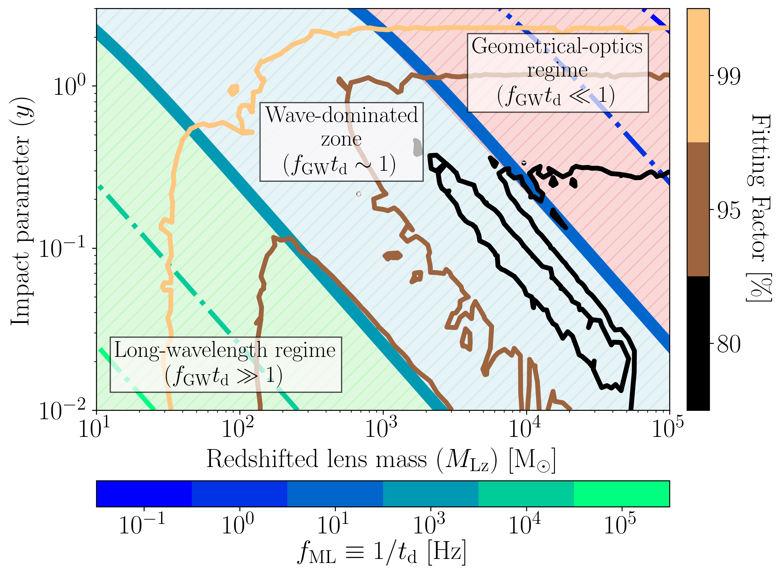
Figure 1: Figure illustrating the contrast in trends between the variation of characteristic micro-lensing frequency, $f_{\rm ML}$, and the fitting factor, $FF$, value when microlensed signals are recovered using unlensed templates. $f_{\rm ML}$ indicates the onset of significant microlensing effects (see Eq. 9), whereas $FF$ is related to the Bayes Factor in favour of microlensing against the unlensed hypothesis (see Eq. 16). The analysis is conducted within the parameter space relevant to isolated point lenses, focusing on the current-generation ground-based detectors. The $f_{\rm ML}$ values are shown in Blue - Green colorbar. Contours at $10$ and $1000$ Hz denote the rough transition regions, dividing the parameter space into three zones. (i) Long-Wavelength Regime where the GW frequency ($f_{\mathrm{GW}}$) is significantly lower than $f_{\mathrm{ML}}$, meaning $f_{\mathrm{GW}}\ll f_{\mathrm{ML}}$, resulting in minimal interaction between GWs and the microlens, as seen from the light green colored region of the figure. (ii) Wave Dominated Zone: This is the region where $f_{\mathrm{GW}}\sim f_{\mathrm{ML}}$, leading to substantial interference effects on GWs, depicted with light blue color. (iii) Geometrical-Optics Regime: The right-most region in the figure is shown with light coral color where $f_{\mathrm{GW}}\gg f_{\mathrm{ML}}$. This region is inclusive of milli-lensing and strong-lensing scenarios. Blue - Green colorbar represent $FF$ contours where the parameters of the source binary are kept fixed to a non-spinning equal mass binary having $60\leavevmode\nobreak\$M_⊙. For each microlensed WF, the $FF$ values are computed by maximizing its match with the unlensed WFs within the parameter space of component masses and aligned spins.

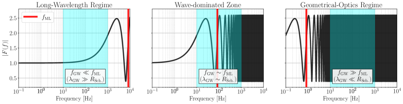
Figure 2: Illustration of the nature of microlensing modulations in the three regimes. The absolute part of the amplification factor, $|F(f)|$, is plotted against frequency (black lines). Microlens parameters are fixed at $y=0.3$ and $M_{\mathrm{Lz}}/{\rm M}_{\odot}\in\{10,\leavevmode\nobreak\ 10^{3},\leavevmode\nobreak\ 10^{5}\}$, arranged from left to right. The blue-shaded region represents the sensitivity band of current ground-based detectors, approximately $10-100\leavevmode\nobreak\$Hz, for reference. The red vertical line indicates the characteristic frequency for the onset of significant microlensing effects, $f_{\mathrm{ML}}$. The panels are divided based on whether $f_{\mathrm{ML}}>1000\leavevmode\nobreak\$Hz (left panel, long-wavelength regime), $f_{\mathrm{ML}}\in(10-1000)\leavevmode\nobreak\$Hz (middle panel, wave-dominated zone), or $f_{\mathrm{ML}}<10\leavevmode\nobreak\$Hz (right panel, geometrical optics regime).

In the case of the isolated point-mass lens model, the time delay between the two (micro) images is determined only by $M_{\mathrm{Lz}}$ and $y$, given by (Schneider and Weiss, 1986; Schneider et al., 1992):

$$t_{\mathrm{d}}(M_{\mathrm{Lz}},\leavevmode\nobreak\ y)=4M_{\mathrm{Lz}}\left[\frac{y+\sqrt{y^{2}+4}}{2}+\ln\left(\frac{\sqrt{y^{2}+4}+y}{\sqrt{y^{2}+4}-y}\right)\right].$$ (5)

By examining how the GW frequency, $f_{\rm GW}$, compares to the time delay caused by the gravitational lens, $t_{\mathrm{d}}$, we can categorize $M_{\mathrm{Lz}}-y$ space into three distinct regimes (Mishra et al., 2023; Bondarescu et al., 2023):

1. Long-wavelength regime: In this regime, $f_{\rm GW}\cdot t_{\mathrm{d}}\ll 1$ ($\lambda_{\mathrm{GW}}\gg R_{\mathrm{Sch}}$), leading to only a minimal interaction between the signal and the lens. The amplification factor in this regime can be approximated as Tambalo et al. (2023):

   $$F(\omega,\leavevmode\nobreak\ y)\simeq 1+\frac{\omega}{2}[\pi-i(2\log(y)-\mathrm{Ei}(i\omega y^{2}/2)]+\mathcal{O}(\omega^{2}),$$ (6)

   where $\mathrm{Ei}(i\omega y^{2}/2)$ is the exponential integral. Note that, in the leading order, $F(\omega,\leavevmode\nobreak\ y)\propto 1+\omega$. Thus, for $\omega\ll 1$, there is no effect of lensing on signals as $F(\omega,\leavevmode\nobreak\ y)=1$. However, as $f_{\rm GW}\cdot t_{\mathrm{d}}$ approaches unity while still being much less than it, the presence of non-zero $\omega$ can lead to a frequency-dependent amplification of the signal. That is why some authors also term this region as the ‘amplification’ regime Bondarescu et al. (2023).

2. Wave-dominated zone: In this zone, $f_{\rm GW}\cdot t_{\mathrm{d}}\sim 1$ (where interference effects will be dominating). This leads to a frequency-dependent modulation of the signal which in case of a point-lens is governed by Eq. 4.

3. Geometrical Optics regime: If $f_{\rm GW}\cdot t_{d}\gg 1$ in Eq. (1), the integral becomes highly oscillatory, and only the stationary point of the integrand have a non-zero contribution to the integral. In such cases, Eq. (1) can be written as

   $$F\left(f\right)\big{|}_{\rm geo}=\sum_{j}\sqrt{|\mu_{j}|}\exp\left(2\pi ift_{\rm d,j}-i\pi n_{j}\right),$$ (7)

   where $\mu_{j}$ and $t_{d,j}$ are, respectively, the magnification factor and the time delay for the $j$-th image. Also, $n_{j}$ is the Morse index, with values 0, 1/2, and 1 for stationary points corresponding to the minima, saddle and maxima of the time-delay surface, respectively. In the case of point mass lens, it reduces to Takahashi and Nakamura (2003)

   $$F(f)=|\mu_{+}|^{1/2}-i|\mu_{-}|^{1/2}e^{i2\pi ft_{\mathrm{d}}},$$ (8)

   where the magnification of each image is $|\mu_{\pm}|=1/2\pm(y^{2}+2)/(2y\sqrt{y^{2}+4})$ and the time delay between the two microimages is given by Eq. 5. Physically, Eq. 8 implies that in the high-frequency limit, the modifications due to a point lens can be considered as a trivial superposition of two signals which differ only by a constant amplitude, a phase shift of $\pi/2$, and a time-delay value smaller than the chirp time of the signal.

One can explicitly find the characteristic frequency $f_{\mathrm{ML}}$ where the wave effects dominate for a given $M_{\mathrm{Lz}}$ and $y$, given by

$$f_{\mathrm{ML}}(M_{\mathrm{Lz}},\leavevmode\nobreak\ y)\equiv\frac{1}{t_{\mathrm{d}}(M_{\mathrm{Lz}},\leavevmode\nobreak\ y)}.$$ (9)

Considering that current ground-based detectors (LIGO and Virgo) are primarily sensitive in the band $\sim(10-1000)\leavevmode\nobreak\$Hz, we can illustrate the variation of $f_{\mathrm{ML}}$ in the $M_{\mathrm{Lz}}-y$ parameter space as shown by contours corresponding to the Blue-Green colorbar in Fig. 1. Here, we roughly demarcate $M_{\mathrm{Lz}}-y$ space based on whether $f_{\mathrm{ML}}>1000\leavevmode\nobreak\$Hz (long-wavelength regime; depicted by light green colored region), $f_{\mathrm{ML}}\in(10,\leavevmode\nobreak\ 1000)\leavevmode\nobreak\$Hz (wave dominated zone; depicted by light blue colored region), or $f_{\mathrm{ML}}<10\leavevmode\nobreak\$Hz (geometrical optics regime; depicted by light coral colored region). Additionally, we also illustrate the variation of the fitting factor $FF$ in the figure, which we discuss later in II.3.3. Throughout this work, we will primarily work within the parameter space range depicted in the figure: $M_{\mathrm{Lz}}/{\rm M}_{\odot}\in(10,\leavevmode\nobreak\ 10^{5})$ and $y\in(0.01,3)$, unless otherwise stated. This parameter space is relevant for searching microlensing signatures due to an isolated point lens in the context of ground-based detectors.

In Fig. 2, we explicitly illustrate the nature of microlensing modulations in the three regimes. The absolute part of the amplification factor, $|F(f)|$, is plotted against frequency (black lines), where the microlens parameters are fixed at $y=0.3$ and $M_{\mathrm{Lz}}/{\rm M}_{\odot}\in\{10,\leavevmode\nobreak\ 10^{3},\leavevmode\nobreak\ 10^{5}\}$, arranged from left to right. The blue-shaded region represents the sensitivity band of current ground-based detectors, $\sim 10-100\leavevmode\nobreak\$Hz, for reference. In the long-wavelength regime (left panel), we observe solely frequency-dependent amplification, as discussed in relation to Eq. 6. Moving to the middle panel, we notice that $f_{\mathrm{ML}}$ indeed marks the point where interference effects begin to dominate. This point typically occurs shortly after the first peak and trough of the amplification factor. It is worth pointing out that the characteristic location of $f_{\mathrm{ML}}$ (lying between the first two peaks) remains consistent across different lensing parameters. In contrast, the right panel illustrates highly oscillatory modulations that eventually lead to an averaging effect (geometrical optics limit). This behavior eventually results in frequency-independent effects.

When significant, microlensing modulations can lead to systematic biases in the estimation of source parameters, especially when the intervening microlens belong to the wave-dominated zone Mishra et al. (2023). When microlensed GW signals are recovered with the usual unlensed GW signals, the phase modulations can bias the inference of intrinsic parameters, especially the in-plane spin components (or precession). Among extrinsic parameters, the recoveries of luminosity distance are affected the most. In contrast, the trigger time and the sky-position parameters, right ascension (RA) and declination (Dec) ($\alpha$ and $\delta$), are the mostly well-recovered source parameters.

The micro-lensing-induced systematic biases could be mistakenly interpreted as evidence of a deviation from GR. This potential misinterpretation arises from the necessity of incorporating micro-lensing effects into the model during the GW signal analysis. Additionally, it is worth noting that the standard tests of GR routinely applied to observed GW signals Abbott et al. (2021e) are liable to a range of systematic effects Narayan et al. (2023); Saini et al. (2022); Bhat et al. (2023). While there have been studies addressing systematic biases that can lead to misinterpretations of GR, the impact of micro-lensing remains unexplored. To address this gap, we conduct an in-depth simulation study, focusing on two theory-agnostic GR tests, to assess how micro-lensing effects may influence the identification of non-GR signatures in observed GW data.

II.2 Tests of General Relativity (TGR)

II.2.1 Inspiral-Merger-Ringdown Consistency Test (IMRCT)

The IMRCT is one of the standard consistency tests of GR that is performed on real GW events. The test relies on checking the consistency between the measurements of mass and spin of the remnant BH inferred independently from the inspiral and post-inspiral parts of the GW signal. The demarcation between the inspiral and the post-inspiral regime is typically done by employing a cutoff frequency $f^{\mathrm{IMR}}_{\mathrm{c}}$ in the frequency domain, which is the dominant mode GW frequency $f_{\mathrm{ISCO}}$ of the innermost stable circular orbit (ISCO) of the remnant Kerr BH with mass $M_{f}$ and dimensionless spin $\chi_{f}$. In this work, the ISCO frequency of the final Kerr black hole is measured using the median values of the 1D-marginalized posteriors of the final mass and spin inferred from the full IMR waveform (Ghosh et al., 2016, 2018). To calculate the final mass and spin, we use the NR-calibrated fits as detailed in Ref. Abbott et al. (2017, 2021d); Johnson-McDaniel et al. where the method extends the final spin fit of aligned-spin binaries to a precessing case (see Eqn. 1 of Ref. Johnson-McDaniel et al. for details).

To elaborate, we independently infer the posterior distributions of $M_{f}$ and $\chi_{f}$ from both the inspiral and the post-inspiral parts of the signal by using the augmented NR calibrated final state fits Hofmann et al. (2016); Jiménez-Forteza et al. (2017); Healy and Lousto (2017). To constrain possible deviations from GR, a set of fractional deviation parameters $\Delta M_{f}/\overline{M}_{f}$ and $\Delta\chi_{f}/\overline{\chi}_{f}$ are defined, where

$$\frac{\Delta M_{f}}{\overline{M}_{f}}\equiv 2\frac{M_{f}^{\mathrm{insp}}-M_{f}^{\mathrm{post-insp}}}{M_{f}^{\mathrm{insp}}+M_{f}^{\mathrm{post-insp}}}$$ (10)

and

$$\frac{\Delta\chi_{f}}{\overline{\chi}_{f}}\equiv 2\frac{\chi_{f}^{\mathrm{insp}}-\chi_{f}^{\mathrm{post-insp}}}{\chi_{f}^{\mathrm{insp}}+\chi_{f}^{\mathrm{post-insp}}},$$ (11)

where $\overline{M_{f}}$ and $\overline{\chi_{f}}$ denote the mean values and the superscripts denote the inspiral (insp) and the post-inspiral (postinsp) portions of the signal. If a given GW signal is consistent with GR, the fractional deviations $\Delta M_{f}/\overline{M}_{f}$ and $\Delta\chi_{f}/\overline{\chi}_{f}$ should vanish in the ideal situation. We estimate the posteriors on these fractional deviation parameters and check the consistency with GR.

To check the consistency of inspiral and post-inspiral measurements statistically, we use the GR quantile $Q_{\rm GR}$. In this case, the GR quantile for the 2-D distribution of final mass and spin parameters measures the fraction of the posterior samples that contain the GR value. Specifically, we utilize the summarytgr executable within PESummary Hoy and Raymond (2021) to calculate the GR deviations. Notice that a smaller value denotes better agreement with GR, meaning that a large fraction of samples are contained in a small iso-probability contour. We use IMRPhenomXPHM Pratten et al. (2021) as our waveform approximant for both injection and recovery of the IMRCT analysis throughout.

II.2.2 Parameterized test

The dynamics of a BBH system can be described in three regimes: the inspiral, the merger and the ringdown. In the inspiral, the post-Newtonian formalism accurately describes the evolution, which is an expansion in the velocity parameter $v/c\ll 1$, where $c$ is the velocity of light Blanchet (2014). In contrast, one needs numerical relativity techniques to model the dynamics towards the merger regime Pretorius (2007); Duez and Zlochower (2019), where the strong-field dynamics play a critical role. In the post-merger phase, BH perturbation theory provides a good description Berti et al. (2006).

Parameterized tests of post-Newtonian (PPN) theory are among the multiple ways of performing theory-agnostic tests of GR. Even though the PPN tests were restricted to the inspiral regime Arun et al. (2006a, b); Agathos et al. (2014), later on, they were also extended to the post-inspiral regime by employing the phenomenological waveform models (Abbott et al., 2019c, 2021d; Meidam et al., 2018; Abbott et al., 2016a, 2019b, 2019c, 2021d). The PPN tests introduce a novel way of looking for deviations in the inspiral-merger-ringdown coefficients from the GR model by appropriately incorporating parameterized deviation coefficients in the model. We denote the inspiral coefficients as $\{\chi_{i}\}$, and the post-inspiral coefficients as $\{\alpha_{i},\beta_{i}\}$, where $\{\beta_{i}\}$ accounts for deviations mainly in the intermediate phase while $\{\alpha_{i}\}$ in the merger-ringdown phase. The parameterized deviations to these coefficients are of the form, $\chi_{i}\rightarrow(1+\delta\hat{\chi}_{i})\chi_{i}$, $\alpha_{i}\rightarrow(1+\delta\hat{\alpha}_{i})\alpha_{i}$ and $\beta_{i}\rightarrow(1+\delta\hat{\beta}_{i})\beta_{i}$, where $\delta\hat{\chi}_{i}$, $\delta\hat{\alpha}_{i}$ and $\delta\hat{\beta}_{i}$ are the fractional deviations from the GR coefficient. In the case of phenomenological waveform models, the post-Newtonian inspiral coefficients are extended further by fitting to numerical relativity coefficients Ajith et al. (2008, 2011); Santamaria et al. (2010); Husa et al. (2016); Khan et al. (2016); García-Quirós et al. (2020); Pratten et al. (2020). Besides the inspiral, the parameters $\delta\hat{\beta}_{i}$ explicitly capture deformations in the NR calibrated coefficients $\beta_{i}$ in the intermediate regime, whereas the parameters $\delta\hat{\alpha}_{i}$ describe deformations of the merger-ringdown coefficients $\alpha_{i}$ obtained by calibration to NR Meidam et al. (2018); Abbott et al. (2019c). The data provide constraints on these parameterized deviations from GR and can be used to test the consistency of GR. That means we obtain posterior probability distributions on each of the parameterized deviation coefficients. If the data is consistent with GR, the distribution will peak at zero, the GR value. Any deviation from GR can hint at the presence of an alternative theory model or missing physics in our models, such as various systematic effects. To quantify such a possible deviation from GR, we use $\sigma_{\rm GR}$, defined as, $\sigma_{\rm GR}=(\mu-\mu_{\rm GR})/\sigma$. Here $\mu$ is the mean of the distribution, $\mu_{\rm GR}$ is the GR value, and $\sigma$ is the standard deviation of the posterior distribution. Since $\mu_{\rm GR}=0$, we simply get $\sigma_{\rm GR}=\mu/\sigma$.

In this study, we restrict to two inspiral coefficients, $\delta\hat{\chi}_{0}$ (0PN) and $\delta\hat{\chi}_{4}$ (2PN), respectively, which appear in the Newtonian and the second post-Newtonian order in the inspiral phase of the waveform. Moreover, we consider two coefficients in the post-inspiral regime: $\delta\hat{\beta}_{2}$ from the intermediate phase and $\delta\hat{\alpha}_{2}$ from the merger-ringdown phase. We employ IMRPhenomPv2 waveform model for this study, which is a dominant-mode model for precessing BBHs where the inspiral coefficients are obtained from PN theory and calibration to NR waveforms, and the post-inspiral coefficients by fitting to NR-simulations Hannam et al. (2014); Husa et al. (2016); Khan et al. (2016); Alejandro et al. . Consequently, the inspiral phase is defined up to a cutoff frequency $f_{\mathrm{cut}}=f^{\mathrm{PAR}}_{\mathrm{c}}=0.018/M$, where $M$ is the total mass of the binary (Husa et al., 2016; Khan et al., 2016).

II.3 GW data analysis and Parameter Estimation Setup

Here we discuss some general tools and setup that are common throughout this work.

II.3.1 Injections

To study the effect of microlensing on the tests of GR using GWs, we consider simulated binary black hole (BBH) events, called injections. These injections are done in the detector network of LIGO-Virgo with the projected O4 sensitivity (Abbott et al., 2020). To avoid noise systematics, i.e., biases due to specific noise realizations, we do not include noise in our injections (assuming the realization of Gaussian noise that yields zero noise in the data containing the signal).

Firstly, in Sect. III.1, we consider a set of $30$ zero-noise microlensed BBH injections, consisting of GW150914-like non-spinning signals with added microlensing effects. The component masses and the extrinsic parameters of the signals are kept similar to those of GW150914, except for the luminosity distance, which is tuned to fix the network optimal signal-to-noise ratio (SNR) to $50$ for each injection in the detector network of advanced LIGO at Hanford, Livingston and, Virgo. In addition, the spin components are kept zero to avoid possible systematic errors in the inference of the deviation parameters from GR and make sure any biases arise predominantly from microlensing effects. This is because one needs to have even higher SNR values of $\gtrsim 10^{2}$ to reliably estimate both the spin components (Pürrer et al., 2017). The microlens parameters used for generating the injections correspond to $\log_{10}M_{\mathrm{Lz}}\in\{1,\leavevmode\nobreak\ 2,\leavevmode\nobreak\ 3,\leavevmode\nobreak\ 4,\leavevmode\nobreak\ 5\}$ and $y\in\{0.01,\leavevmode\nobreak\ 0.05,\leavevmode\nobreak\ 0.1,\leavevmode\nobreak\ 0.5,\leavevmode\nobreak\ 1.0,\leavevmode\nobreak\ 3.0\}$, making $30$ injections in total.

In Sect. III.2, to robustly analyze the effect of microlensing on tests of GR, we consider a population of simulated microlensed signals. We generate a mock GW data set of $\sim 2.5\times 10^{4}$ microlensed BBH signals, where the mass and spin priors are derived from the inferred population model of GWTC-3 data (Abbott et al., 2021c): the source-frame component masses are sampled from the Power Law + Peak distribution and spin parameters are drawn from a Gaussian isotropic distribution. We assume the Madau-Dickison profile for the merger rate density in the universe (Madau and Dickinson, 2014; Fishbach et al., 2018), with the source redshift range set to $z_{\mathrm{S}}\in(0.001,\leavevmode\nobreak\ 10)$. The upper limit of $z_{\rm S}=10$ is set because isolated point lenses tend to amplify the signals, increasing their optimal SNR and, consequently, their detection horizon Mishra et al. (2023). To sample microlens parameters, we assume a log-uniform prior in $M_{\mathrm{Lz}}$ and a linear power-law prior for $y$, where:

$$p(\log_{10}M_{\mathrm{Lz}}) \propto\text{Uniform}(1,\leavevmode\nobreak\ 5),$$ (12)

$$p(y) \propto y,\leavevmode\nobreak\ \leavevmode\nobreak\ y\in(0.01,\leavevmode\nobreak\ 3.00).\$$

The motivation to use $p(y)\propto y$ comes from geometry and isotropy (Lai et al., 2018). The other parameters were sampled from the usual prior distributions: isotropic sky location and orientation, and uniform polarization angle. We put an observed network SNR, $\rho_{\mathrm{opt}}^{\rm N}$, threshold of $8$ when using the unlensed templates for recovery in the LIGO-Virgo detector network. We further impose an additional requirement that $\mathrm{SNR}>6$ in both the inspiral and post-inspiral parts of the signal. This requirement ensures that we have an adequate amount of information for our analyses in both signal regimes. The demarcation between these two regimes is done via a cutoff frequency $f_{\mathrm{cut}}$ in the frequency domain. We define $f_{\mathrm{cut}}=f_{\mathrm{ISCO}}$ for IMRCT and $f_{\mathrm{cut}}=f_{\mathrm{C}}^{\mathrm{PAR}}$ for the parameterized test, as explained in Sect. II.2. For performing IMRCT, these SNR thresholds are consistent with the previous analyses Abbott et al. (2021e, d). However, we note that for parameterized tests, our SNR thresholds are stricter. For example, to study the deviations in the coefficients corresponding to the inspiral regime, such as $\delta\hat{\chi}_{0}$ and $\delta\hat{\chi}_{4}$ considered here, one only needs to have the inspiral $\mathrm{SNR}>6$. A stricter condition of $\mathrm{SNR}>6$ in both the inspiral and post-inspiral regimes is employed so that each injection can be analyzed for all four testing GR parameters.

II.3.2 Parameter Estimation

Throughout this work, we use the publicly available Bayesian inference library Bilby Ashton et al. (2019) for performing parameter estimation runs. Specifically, we use the dynesty Speagle (2020) nested sampler with the ‘acceptance-walk’ method for the Markov-Chain Monte-Carlo (MCMC) evolution as implemented in Bilby, along with the sampler settings of nlive$=1024$, n-accept$=60$ and n-parallel$=2$ per injection. The lower frequency limit of the likelihood evaluation is set to $f_{\mathrm{low}}=20\leavevmode\nobreak\$Hz, which is also the reference frequency.

Furthermore, in order to compute microlensing effects, whether for generating microlensed injections or inferring microlens parameters, we employ a custom frequency domain source model, which incorporates the two microlensing parameters $M_{\mathrm{Lz}}$ and $y$ in addition to the standard 15 BBH parameters and is made publicly available via Python/Cython package GWMAT (Mishra, A., 2023, in prep.).

While inferring microlens parameters in our simulated microlensed signals with injected $M_{\mathrm{Lz}}\equiv M_{\mathrm{Lz}}^{\mathrm{true}}$ and $y\equiv y^{\mathrm{true}}$, we assume a log-uniform prior in $M_{\mathrm{Lz}}$ and a linear power-law prior for $y$, where:

$$p(\log_{10}M_{\mathrm{Lz}})\propto\begin{cases}\text{Uniform}(-1,\leavevmode\nobreak\ 5),&\text{if }\log_{10}M_{\mathrm{Lz}}^{\mathrm{true}}<3\\ \text{Uniform}(-1,\leavevmode\nobreak\ 7),&\text{otherwise}\end{cases}$$ (13)

$$p(y)\propto y,\text{where}\begin{cases}y\in(0.001,\leavevmode\nobreak\ 3.00),&\text{when }y^{\mathrm{true}}<1\\ y\in(0.001,\leavevmode\nobreak\ 5.00),&\text{otherwise. }\end{cases}$$ (14)

We also use these priors while generating a population of microlensed signals.

For the parameterized test of GR, we independently vary each of the four deviation parameters instead of simultaneously varying them, aligning with the methodology employed in the LVK catalog analyses (Abbott et al., 2021d, e) and similar studies (Narayan et al., 2023). However, we do note that in an alternative theory of gravity, one would anticipate modifications to all post-Newtonian (PN) coefficients beyond a certain order. This choice of varying only one parameter at a time is made to avoid uninformative results, as observed in cases where multiple parameters are allowed to vary simultaneously, as illustrated for $\mathrm{GW150914}$ in Abbott et al. (2016a). Nevertheless, earlier studies (Meidam et al., 2018; Johnson-McDaniel et al., 2022) have demonstrated that even when varying a single testing parameter, it is still possible to detect deviations from GR that modify multiple PN coefficients (even when this testing parameter is itself not modified).

II.3.3 Model Comparison

To study whether a given GW event is microlensed or not, one can analyze the data under the assumption of two hypotheses: (i) Null-hypothesis $\mathcal{H}_{\mathrm{UL}}$: the signal is unlensed, , and (ii) $\mathcal{H}_{\mathrm{ML}}$: the signal is microlensed. Under the assumption that the two models are equally likely, we set their prior probabilities to be equal (i.e., $p(\mathcal{H}_{\mathrm{UL}})=p(\mathcal{H}_{\mathrm{ML}})$). One then compares the two models using the Bayes factor formalism, where the Bayesian evidence (or marginal likelihood) $\mathcal{Z}$ of $\mathcal{H}_{\mathrm{ML}}$ is compared against that of $\mathcal{H}_{\mathrm{UL}}$, given by

$$\mathcal{B}^{\mathrm{ML}}_{\mathrm{UL}}\equiv\frac{p(\mathcal{H}_{\mathrm{ML}}|\mathcal{D})}{p(\mathcal{H}_{\mathrm{UL}}|\mathcal{D})}=\frac{\mathcal{Z}_{\mathrm{ML}}}{\mathcal{Z}_{\mathrm{UL}}},$$ (15)

where $\mathcal{D}$ represents data. As mentioned in the previous subsection II.3.2, we utilize the dynesty Speagle (2020) nested sampler as implemented in Bilby (Ashton et al., 2019) to compute both the Bayesian evidence and inferring parameters, unless otherwise noted. However, since computing Bayesian evidence using a nested sampling algorithm is usually computationally expensive, one can also employ an estimation method (Cornish et al., 2011; Vallisneri, 2012) for sufficiently high SNR values, where the leading order term in (log) Bayes factor can be expressed as

$$\log_{10}\mathcal{B}^{\mathrm{ML}}_{\mathrm{UL}}\approx\frac{1}{2\ln{10}}\rho_{\mathrm{res}}^{2}.$$ (16)

Here, $\rho_{\mathrm{res}}^{2}=(1-FF^{2})\rho_{\mathrm{ML}}^{2}$ represents the SNR of the residual waveform after the best fit unlensed waveform has been subtracted out from the true microlensed WF. $\rho_{\mathrm{ML}}$ is the SNR when the true microlensed waveform is used to extract the signal, and $FF$ represents the fitting factor value (Sathyaprakash and Dhurandhar, 1991; Ajith et al., 2014), indicating the match between the best-fit unlensed waveform and the true microlensed waveform (or equivalently, $FF=\rho_{\mathrm{UL}}/\rho_{\mathrm{ML}}$). The match $\mathfrak{M}$ between two waveforms, $h_{1}(t)$ and $h_{2}(t)$, is defined as the noise-weighted inner product, maximized over phase $(\phi)$ and time $(t)$:

$$\mathfrak{M}(h_{1},h_{2}) \equiv\underset{t,\phi}{\mathrm{max}}\bra{h_{1}}\ket{h_{2}}$$ (17)

$$\equiv\underset{t,\phi}{\mathrm{max}}\leavevmode\nobreak\ 4\mathcal{R}\int_{f_{\mathrm{low}}}^{f_{\mathrm{high}}}df\frac{\tilde{h}_{1}^{*}(f)\tilde{h}_{2}(f)}{S_{\mathrm{n}}(f)}\cdot e^{i(2\pi ft+\phi)},$$

where $f_{\mathrm{low}}$ and $f_{\mathrm{high}}$ are the lower and upper-frequency cutoffs of the integral. Here, the tilde represents the Fourier transform, the asterisk denotes the complex conjugate, and $S_{\mathrm{n}}(f)$ is the one-sided noise power spectral density (PSD). We only employ this estimation method when we study a population of $\mathcal{O}(10^{4})$ signals in Sect. III.2.1.

In Fig. 1, in addition to showing the trend of $f_{\mathrm{ML}}$, we also illustrate the trend of variation of $FF$ in the $M_{\mathrm{Lz}}-y$ parameter space. For each microlensed signal, the binary parameters are kept fixed to a non-spinning equal mass binary having $60\leavevmode\nobreak\$M_⊙, and the $FF$ value is obtained by maximizing the match between the microlensed WF and the 4-dimensional aligned-spin template WFs, modelled by the two component masses and their aligned spins. The match is maximized using the Nelder-Mead algorithm as implemented in the ‘optimization’ module of the Scipy library (Virtanen et al., 2020). As we can see, the trend of variation of $FF$ is different from that of the variation of $f_{\mathrm{ML}}$. Notably, the $FF$ values roughly increase as we move towards the bottom-right corner of the parameter space, with increasing $M_{\mathrm{Lz}}$ and $1/y$ values. Conversely, the $f_{\mathrm{ML}}$ values increase as we move from the top-right corner of the $M_{\mathrm{Lz}}-y$ parameter space towards the bottom-left corner. It is important to note that the region where wave effects dominate differs from the area associated with low match values (high Bayes factor values in favour of microlensing). This observation plays a crucial role in the interpretation of our results.

It is important to note that the region where wave effects dominate differs from the area associated with low match values (high Bayes factor values in favour of microlensing). This observation plays a crucial role in the interpretation of our results.

III Results and Discussions

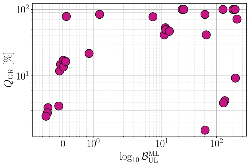
(a) $\mathcal{B}^{\mathrm{ML}}_{\mathrm{UL}}$ vs. $Q_{\mathrm{GR}}$

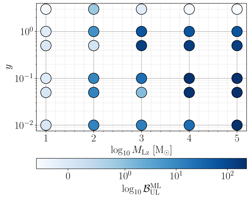
(b) $\log_{10}\mathcal{B}^{\mathrm{ML}}_{\mathrm{UL}}$ dependence on $M_{\mathrm{Lz}}$-$y$ parameter space.

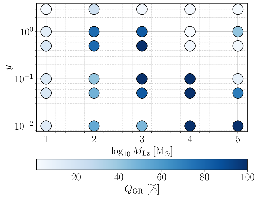
(c) $Q_{\mathrm{GR}}$ dependence on $M_{\mathrm{Lz}}$-$y$ parameter space.

Figure 3: IMRCT results for GW150914-like microlensed injections, highlighting deviations from GR ($Q_{\mathrm{GR}}$), alongside the microlensing Bayes factor ($\log_{10}\mathcal{B}^{\rm ML}_{\rm UL}$) for reference.

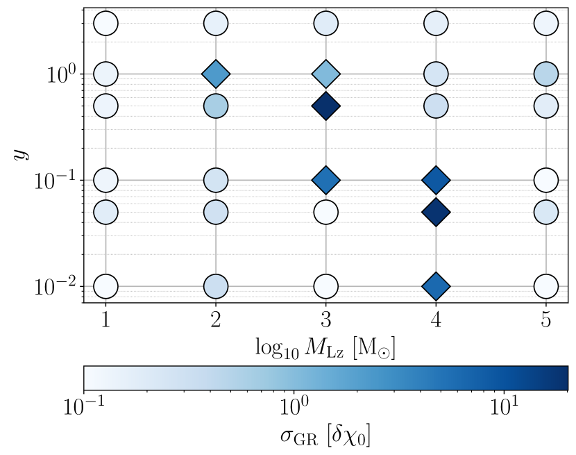
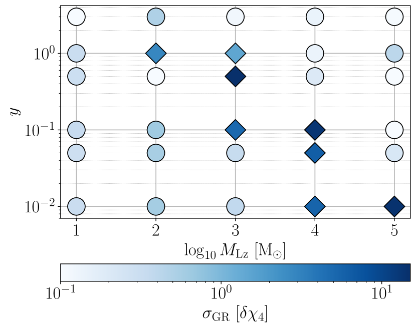
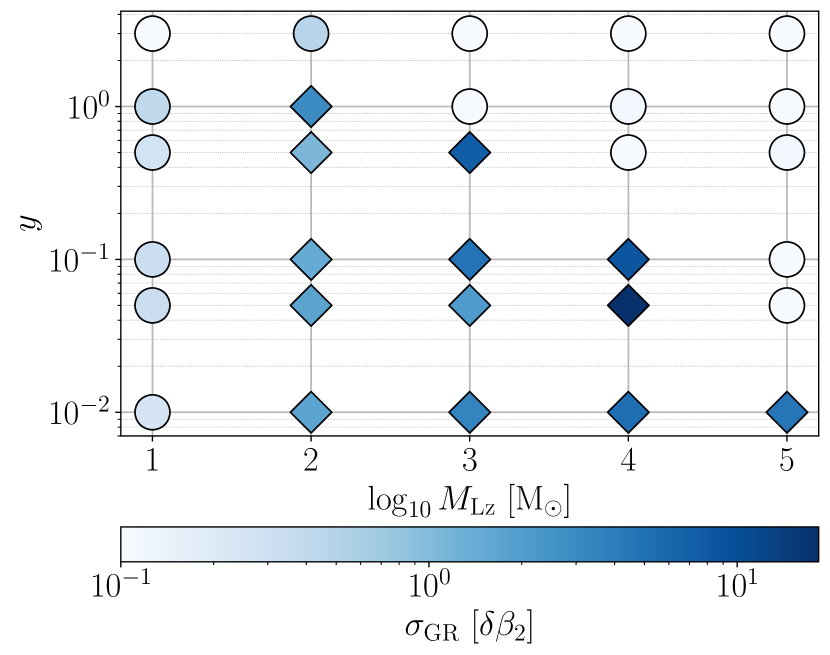
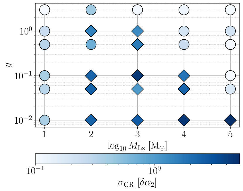
Figure 4: Bias in the parameterized test of GR in GW150914-like microlensed injections for four deviation parameters $\{\delta\hat{\chi}_{0},\leavevmode\nobreak\ \delta\hat{\chi}_{4},\leavevmode\nobreak\ \delta\hat{\alpha}_{2},\leavevmode\nobreak\ \delta\hat{\beta}_{2}\}$. Each of the four panels displays the Gaussian sigma values at which GR is excluded ($\sigma_{\mathrm{GR}}$) in one of the four parameterized parameters, as indicated in the colorbar, within the $\log_{10}M_{\mathrm{Lz}}-y$ parameter space. The larger the magnitude of $\sigma_{\mathrm{GR}}$, the greater the significance of deviations from GR. For better visualization, we mark the cases with significant deviations ($\sigma_{\mathrm{GR}}>1$) using a diamond marker instead of the circular markers.

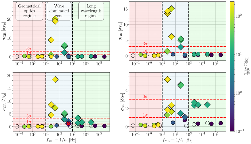
Figure 5: Similar to Fig. 4, but with $M_{\mathrm{Lz}}-y$ parameter space suppressed into a one-dimensional representation using $f_{\mathrm{ML}}$ (see Eq. 9). The figure highlights three scenarios: the long-wavelength regime, the wave-dominated zone, and the geometrical optics regime. The colormap represents $\log_{10}\mathcal{B}^{\rm ML}_{\rm UL}$ values for each injection. Transparent markers with black edges indicate cases where $\log_{10}\mathcal{B}^{\rm ML}_{\rm UL}<0$. Dotted-red lines indicate the $1\sigma$ and $3\sigma$ significance of deviations. Diamond markers indicate significant deviations $(\sigma_{\mathrm{GR}}>1)$, and cases meeting $\log_{10}\mathcal{B}^{\rm ML}_{\rm UL}<1$ (indicating stealth bias) have an added red cross.

III.1 GW150914-like Microlensed Injections

As described in Sect. II.3.1, here we consider zer-noise GW150914-like non-spinning injections with added microlensing effects. The microlens parameters used for generating the injections correspond to $\log_{10}M_{\mathrm{Lz}}\in\{1,\leavevmode\nobreak\ 2,\leavevmode\nobreak\ 3,\leavevmode\nobreak\ 4,\leavevmode\nobreak\ 5\}$ and $y\in\{0.01,\leavevmode\nobreak\ 0.05,\leavevmode\nobreak\ 0.1,\leavevmode\nobreak\ 0.5,\leavevmode\nobreak\ 1.0,\leavevmode\nobreak\ 3.0\}$, making $30$ injections in total. These ideal microlensed BBH injections serve as our initial motivation for the exploration of microlensing-induced biases in tests of GR and enable us to search for patterns in the distortions, helping us identify the intriguing microlensing parameter space where deviations become more prominent.

III.1.1 IMRCT

We conduct six sets of parameter estimation runs for all the $30$ microlensed injections. In the case of IMRCT, each set includes runs for the inspiral part, post-inspiral part, and the full IMR signal, for both unlensed and microlensed hypotheses. The inspiral and post-inspiral regions of our injections are demarcated by the cutoff frequency of $f^{\mathrm{IMR}}_{\mathrm{c}}=f_{\mathrm{ISCO}}=128\leavevmode\nobreak\$Hz.

In Figure 3, we present the results of the IMR consistency test for GW150914-like microlensed injections. We focus on identifying deviations from GR using the GR quantile value, denoted as $Q_{\mathrm{GR}}$. We also illustrate the logarithmic Bayes factor $\log_{10}\mathcal{B}^{\rm ML}_{\rm UL}$ in favor of the microlensed hypothesis over the unlensed hypothesis for the full IMR signal, for reference. Firstly, in Figure 3(a), we depict the relationship between $Q_{\mathrm{GR}}$ and $\log_{10}\mathcal{B}^{\rm ML}_{\rm UL}$. We immediately observe that microlensing effects can introduce bias in the IMR consistency test, resulting in high $Q_{\mathrm{GR}}$ values that surpass $90\%$ in some cases. However, despite noting several occurrences of high $Q_{\mathrm{GR}}$ values $(>70\%)$ when $\log_{10}\mathcal{B}^{\rm ML}_{\rm UL}$ is also high $(>1)$, we do not discern any significant correlation between the two quantities. In other words, there are instances where $\log_{10}\mathcal{B}^{\rm ML}_{\rm UL}$ is low ($<1$), yet $Q_{\mathrm{GR}}$ is high ($>70\%$), and vice versa, where $Q_{\mathrm{GR}}$ is low ($<10\%$), even when $\log_{10}\mathcal{B}^{\rm ML}_{\rm UL}$ is high ($>1$).

Upon closer inspection, we find that the dependence of $Q_{\mathrm{GR}}$ and $\log_{10}\mathcal{B}^{\rm ML}_{\rm UL}$ values on the $M_{\mathrm{Lz}}-y$ parameter space shows a characteristic trend that is notably different between the two (see Figs. 3(b) and 3(c)). Specifically, $\log_{10}\mathcal{B}^{\rm ML}_{\rm UL}$ adheres to the expected behavior, monotonically increasing as we increase the lens mass while reducing the impact parameter. For instance, in Fig. 3(c), the $\log_{10}\mathcal{B}^{\rm ML}_{\rm UL}$ is negative where the microlensing effects are weak (for injections having either $\log_{10}M_{\mathrm{Lz}}=1$ or $y=3$) and increases as we move towards the bottom-right region in the $\log_{10}M_{\mathrm{Lz}}-y$ plane, where it reach values $\mathcal{O}(10^{2})$, indicating strong preference for microlensing. In contrast, the variation in the $Q_{\mathrm{GR}}$ values does not mirror the trend as exhibited by $\log_{10}\mathcal{B}^{\rm ML}_{\rm UL}$, as significant $Q_{\mathrm{GR}}$ values (exceeding $50\%$) are primarily confined within a diagonal region spanning from the top-left to the bottom-right corner. Within the diagonal region, the $Q_{\mathrm{GR}}$ values are high for high lens mass and low impact parameters (bottom-right region of the diagonal) and decrease as we move up in the diagonal towards the top-left direction.

As shown in Figure 1 and elaborated upon in Sect. II.1, the diagonal region in the $\log_{10}M_{\mathrm{Lz}}-y$ parameter space corresponds to the range where wave effects dominate within the sensitivity band of ground-based detectors. In practical terms, the microlens parameters lying in this diagonal region would lead to interference patterns for signals in the frequency range of roughly $10$-$1000\leavevmode\nobreak\$Hz. We observe that $Q_{\mathrm{GR}}$ is significant primarily within the ‘wave-dominated zone’ and decreases as it moves toward the ‘long-wavelength regime’. Conversely, in the ‘geometric-optics regime’ (the parameter space where the geometric-optics approximation tends to hold), we often encounter cases where deviations from GR are minimal ($Q_{\mathrm{GR}}<10\%$) albeit the lensing effects being very high $\log_{10}\mathcal{B}^{\rm ML}_{\rm UL}\sim\mathcal{O}(10)$.

Therefore, from Fig. 3(c), it is evident that deviations from GR appear to occur primarily when interference effects are pronounced. We will further validate this claim using a parameterized test as well as by studying a simulated population similar to GWTC-3 in the following sections.

III.1.2 Parameterized test of GR

To further investigate the apparent deviation from GR due to microlensing effects in the inspiral, intermediate, and merger-ringdown phases of the signal, we perform the parameterized test of GR on our microlensed injection set. As discussed in Sect. II.2.2, we utilize four parameterization variables: $\delta\hat{\chi}_{0}$, $\delta\hat{\chi}_{4}$, $\delta\hat{\beta}_{2}$, and $\delta\hat{\alpha}_{2}$.

In Fig. 4, we show the results of the parameterized test conducted on our microlensed injection set. Each of the four panels displays the Gaussian sigma values at which GR is excluded ($\sigma_{\mathrm{GR}}$; see Sect. II.2.2) in one of the four parameterized parameters, as indicated in the colorbar, within the $\log_{10}M_{\mathrm{Lz}}-y$ parameter space. The larger the magnitude of $\sigma_{\mathrm{GR}}$, the greater the significance of deviations from GR. For better visualization, we mark the cases with significant deviations ($\sigma_{\mathrm{GR}}>1$) using a diamond marker instead of the circular markers. For all four parameters, we observe that the deviations are primarily significant within the wave-dominated zone and gradually decay as we move further into the long-wavelength regime. Meanwhile, the geometrical optics regime doesn’t give any significant deviations. This pattern resembles our observation of the $Q_{\mathrm{GR}}$ value in Fig. 3(c).

To robustly illustrate the relationship between the deviations from GR and the characteristic frequency $f_{\mathrm{ML}}$ at which wave effects caused by a microlens are expected to become more pronounced, we suppress the two-dimensional parameter space of $M_{\mathrm{Lz}}-y$, shown in Fig. 4, into a one-dimensional representation using $f_{\mathrm{ML}}$. We then represent the sigma deviation values in Fig. 5, explicitly emphasizing three distinct regions: the long-wavelength regime, the wave-dominated zone, and the geometrical-optics regime. Moreover, we also depict the $\log_{10}\mathcal{B}^{\rm ML}_{\rm UL}$ values for each injection using a colormap for comparison between the deviations from GR with the overall strength of microlensing. The transparent markers that are not colored and only contain a black edge (unfilled circles) are cases where $\log_{10}\mathcal{B}^{\rm ML}_{\rm UL}<0$ are cases where $\log_{10}\mathcal{B}^{\rm ML}_{\rm UL}<0$. We also mark the $1\sigma$ and the $3\sigma$ deviations with dotted-red lines for better visualization.

For all four parameters, we clearly observe that the deviations from GR primarily increase in the wave-dominated zone (blue shaded region in the middle of each panel), including several cases with $\sigma_{\mathrm{GR}}\gtrsim 5$ for all the parameters. Similarly, within the long-wavelength regime, we only observe significant deviations ($\sigma_{\mathrm{GR}}>1$) for parameters that measure deviations in the post-inspiral regime, i.e., $\delta\hat{\alpha}_{2}$ and $\delta\hat{\beta}_{2}$, where we also observed slight deviations around the intersection of the wave-dominated zone and the long-wavelength regime (also see Appendix B). Within the geometrical-optics regime, we do not notice any significant deviations for any parameter despite encountering several cases with high values of $\log_{10}\mathcal{B}^{\rm ML}_{\rm UL}$, including values $\mathcal{O}(10^{2})$.

It’s also worth noting that in all cases where high biases are observed ($\sigma_{\mathrm{GR}}>3$), we consistently find a high Bayes factor ($\log_{10}\mathcal{B}^{\rm ML}_{\rm UL}>1$) in favor of microlensing. Conversely, there is only a single instance (marked with a red cross in the bottom-left panel) where significant biases are present ($1<\sigma_{\mathrm{GR}}<3$), but the Bayes factor remains notably low ($\log_{10}\mathcal{B}^{\rm ML}_{\rm UL}<0.5$). This suggests that events showing high deviations ($\sigma_{\mathrm{GR}}>3$) from GR must also be analyzed for the presence of microlensing features before claiming any (erroneous) GR deviations. However, to establish this conclusion more firmly, we conduct a more robust study using a population of microlensed signals, as detailed in Section III.2.2.

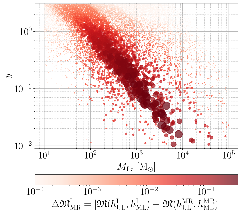
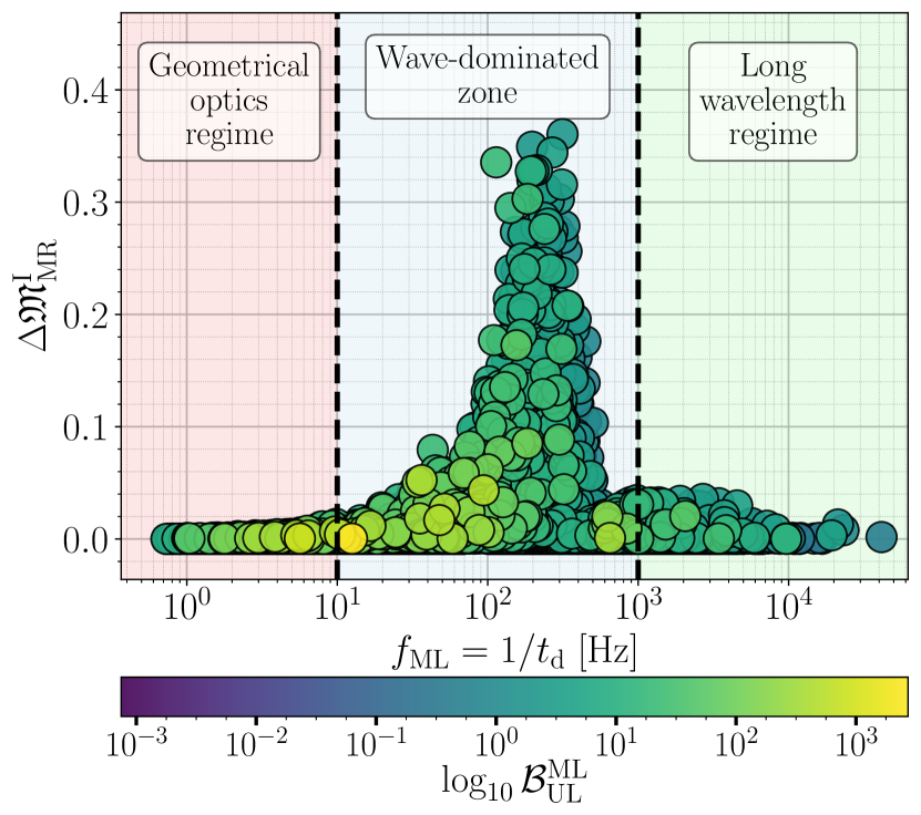
Figure 6: IMRCT results for a population of simulated microlensed injections using $\Delta\mathfrak{M}^{\mathrm{I}}_{\mathrm{MR}}$ (Eq. 18) as a proxy to quantify deviations in IMRCT. Top panel: Depicts $\Delta\mathfrak{M}^{\mathrm{I}}_{\mathrm{MR}}$ in the $\log_{10}M_{\mathrm{Lz}}-y$ parameter space. Marker color and size represent the strength of $\Delta\mathfrak{M}^{\mathrm{I}}_{\mathrm{MR}}$. Bottom panel: Depicts $\Delta\mathfrak{M}^{\mathrm{I}}_{\mathrm{MR}}$ as a function of $f_{\mathrm{ML}}$. The colorbar represents Bayes factor values $\log_{10}\mathcal{B}^{\mathrm{ML}}_{\mathrm{UL}}$ estimated using Eq. 16.

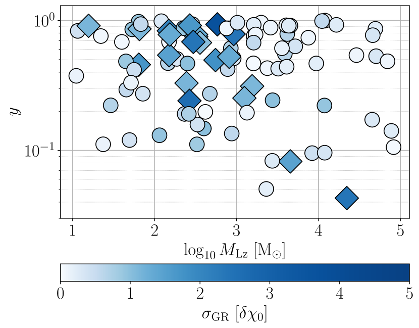
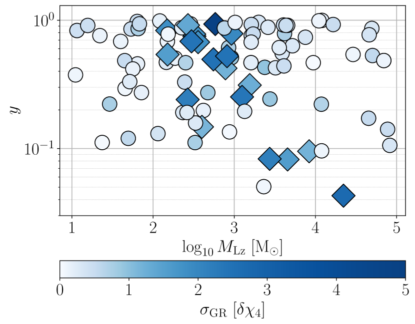
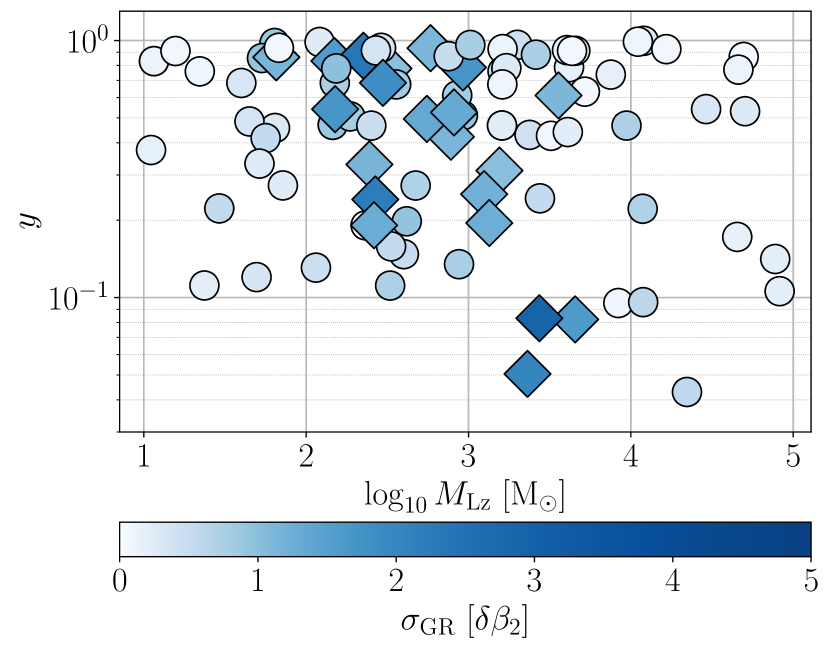
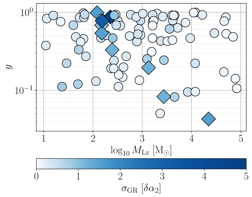
Figure 7: Same as Fig. 4, but for a population of microlensed injections as studied in Sect. III.2.2.

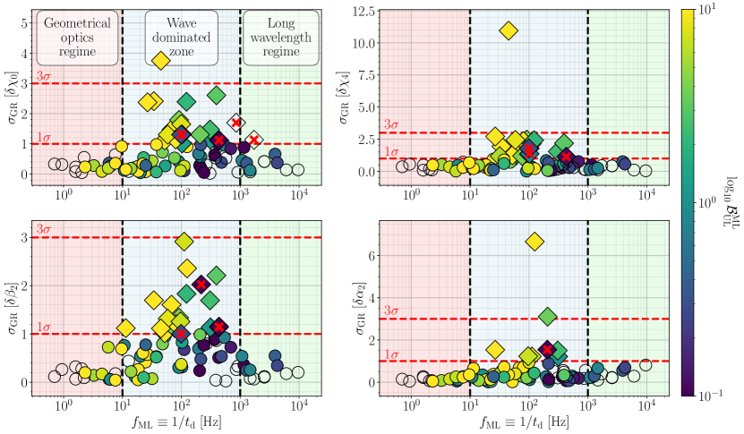
Figure 8: Same as Fig. 5, but for a population of microlensed injections as studied in Sect. III.2.2.

III.2 Population of Microlensed Injections

To robustly analyze the effect of microlensing on tests of GR, we consider a population of simulated microlensed signals (see Sect. II.3.1 for details).

III.2.1 IMRCT

For the study of IMRCT on our microlensed injections, we only consider a subset of those having total mass in the range $50-100\leavevmode\nobreak\$M_⊙, to which our detectors are sensitive from inspiral to ringdown phase of the coalescence (also called “golden" binaries). This leaves us with a total of $\sim 1.5\times 10^{4}$ injections.

Unlike our strategy in Sect III.1.1, we do not perform parameter estimation for this study. We save the computational expense of performing parameter estimation runs by instead studying a quantity that closely resembles the deviation parameter $Q_{\mathrm{GR}}$ in IMRCT. We realize from our study of GW150914-like injections in Sect. III.1.1 that, for IMRCT, the $Q_{\mathrm{GR}}$ value shows a positive correlation with the difference in the match between the microlensed and unlensed waveforms in the inspiral and post-inspiral phases, respectively. In quantitative terms, we observe that the quantity:

$$\Delta\mathfrak{M}^{\mathrm{I}}_{\mathrm{MR}}=|\mathfrak{M}(h_{\mathrm{UL}}^{\mathrm{I}},h_{\mathrm{ML}}^{\mathrm{I}})-\mathfrak{M}(h_{\mathrm{UL}}^{\mathrm{MR}},h_{\mathrm{ML}}^{\mathrm{MR}})|,$$ (18)

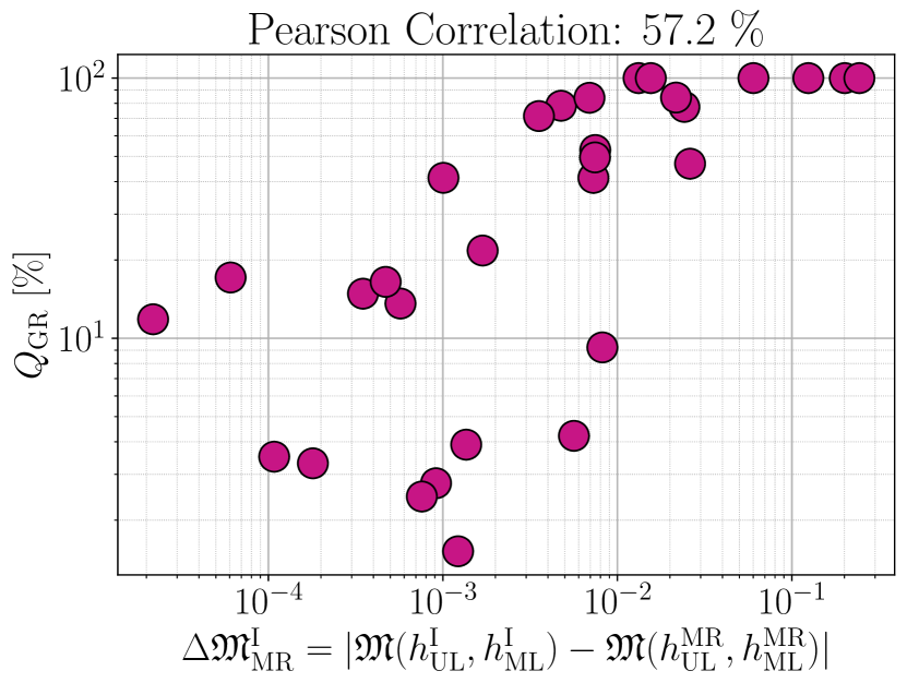
Figure 12: Illustration of correlation between $\mathcal{Q}_{\mathrm{GR}}$ and $\Delta\mathfrak{M}^{\mathrm{I}}_{\mathrm{MR}}$.

where $\mathfrak{M}$ represents match as defined in Eq. 17 , shows a positive Pearson correlation value of around $\sim 57\%$ with $Q_{\mathrm{GR}}$ (see Fig. 12 ). Hence, we compute this quantity for our population as a computationally more cost-effective alternative for estimating the trend of the $Q_{\mathrm{GR}}$ value in IMRCT.

The results are shown in Fig. 6. In the top panel, we depict the quantity $\Delta\mathfrak{M}^{\mathrm{I}}_{\mathrm{MR}}$ in the parameter space of $\log_{10}M_{\mathrm{Lz}}$ and $y$. Both color and size of the markers are proportional to the strength of $\Delta\mathfrak{M}^{\mathrm{I}}_{\mathrm{MR}}$. In other words, markers with dark red color and relatively larger size represent regions where we expect IMRCT to be biased due to microlensing. We again observe that deviations from GR are prominent mainly in the wave-dominated zone. This is more explicitly shown in bottom panel, where we plot the deviation parameter $\Delta\mathfrak{M}^{\mathrm{I}}_{\mathrm{MR}}$ as a function of $f_{\mathrm{ML}}$. We also color the markers based on their Bayes factor values $\log_{10}\mathcal{B}^{\mathrm{ML}}_{\mathrm{UL}}$, estimated using Eq. 16. We clearly see deviations to increase sharply in the wave-dominated zone. In the geometrical-optics regime and the transition region from the wave-dominated to geometrical-optics regime, we again notice several cases having high $\log_{10}\mathcal{B}^{\mathrm{ML}}_{\mathrm{UL}}$ values but with no significant $\Delta\mathfrak{M}^{\mathrm{I}}_{\mathrm{MR}}$ value. These results are consistent with our observations in the previous sections.

III.2.2 Parameterized test of GR

To get a population-wide behavior of deviations in the parameterized test of GR, we choose $100$ injections from our population of microlensed signals. To ensure a significant number of events strongly favors microlensing, we restrict the injected impact parameter value to be less than unity (i.e., $y<1$). Furthermore, the selection employs Eq. 16 to determine $\log_{10}\mathcal{B}^{\mathrm{ML}}_{\mathrm{UL}}$. Since this estimation is not reliable at lower SNRs, we keep the threshold on $\log_{10}\mathcal{B}^{\mathrm{ML}}_{\mathrm{UL}}>9$ for the majority of events $(\sim 50\%)$ (Mishra et al., 2023). The rest of the population corresponds to cases where microlensing is too weak to be correctly identified in the model selection process. Such a population of weakly microlensed signals help us in investigating the possibility of stealth bias (Cornish et al., 2011; Vallisneri, 2012; Vitale and Del Pozzo, 2014) in the context of microlensing - cases where microlensing itself is not large enough to be detectable but the systematic errors due to it remain significant (i.e., larger than the statistical uncertainties in parameter estimation), appearing as deviations from GR.

As discussed in Sect. II.2.2, we study the deviations in each of the four deviation parameters $(\delta\hat{\chi}_{0},\leavevmode\nobreak\ \delta\hat{\chi}_{4},\leavevmode\nobreak\ \delta\hat{\alpha}_{2},\leavevmode\nobreak\ \delta\hat{\beta}_{2})$ separately. The results are plotted in Fig. 7 and Fig. 8, in a similar fashion as in Sect. III.1.2. Particularly, in Fig. 7, we plot the Gaussian sigma deviations in the parameter space of $M_{\mathrm{Lz}}-y$. We again show the cases having $\sigma_{\mathrm{GR}}>1$ with a diamond marker for better visualization. As we can see, there are several cases that give significant deviation from GR $(\sigma_{\mathrm{GR}}>1)$. These include cases that lie in the modest regime in our parameter space, i.e., having the characteristic impact parameter value of $y\approx 1$ and the lens mass $M_{\mathrm{Lz}}<100\leavevmode\nobreak\$M_⊙.

Meanwhile, in Fig. 8, we plot it against the $f_{\mathrm{ML}}$ with colors representing the Bayes factor $\log_{\mathrm{10}}\mathcal{B}^{\mathrm{ML}}_{\mathrm{UL}}$ values obtained via nested sampling. We also put an upper cap of $10$ on the colorbar to get a better visibility of Bayes factors around unity. We observed several instances where $\sigma_{\mathrm{GR}}>1$ for all the parameters, including cases where it is even beyond $3\sigma_{\mathrm{GR}}$. However, we only saw two cases having $\sigma_{\mathrm{GR}}>5$, one for $\delta\hat{\chi}_{4}$ and the other for $\delta\hat{\alpha}_{2}$. We clearly see that deviations increase pre-dominantly in the wave-dominated zone and fall off as we go further into the long-wavelength regime. We do not see any deviation from GR in the geometrical optics regime. These results are consistent with all our previous observations.

To investigate the possibility of stealth bias, we specifically identify cases with significant deviations from GR ($\sigma_{\mathrm{GR}}>1$) but without a strong preference for the microlensing model ($\log_{10}\mathcal{B}^{\mathrm{ML}}_{\mathrm{UL}}<1$), marking them with a red cross. It is worth noting that although several such cases are found, none reach the ’evidence’-level significance ($\sigma_{\mathrm{GR}}>3$). This is because all cases with $\sigma_{\mathrm{GR}}>3$ also exhibit a strong preference for the microlensing hypothesis over the null hypothesis ($\log_{10}\mathcal{B}^{\mathrm{ML}}_{\mathrm{UL}}>1$).

IV Conclusion

In this study, we examined the potential impact of microlensing effects on tests of GR. We adopted an isolated point-lens model for our study, covering a parameter space typically relevant for the ground-based detectors, i.e., $M_{\mathrm{Lz}}\in(1,10^{5})\leavevmode\nobreak\$M_⊙ and $y\in(0.01,3)$. However, it is important to note that our findings and conclusions are expected to apply broadly to any microlensing scenario, regardless of the specific parameter space, as we relate the biases observed to the fundamental characteristic of gravitational lensing. Our investigation centered on two theory-agnostic tests of GR: the inspiral-merger-ringdown consistency test (IMRCT) and the parameterized tests of GR. These tests allowed us to explore deviations from GR across different evolutionary phases of a GW signal: inspiral, intermediate, and merger-ringdown. We consider both high-SNR GW150914-like systems and a population of microlensed signals similar to GWTC-3 with added microlensing effects.

Our findings lead to the following conclusions:

1. Microlensing can significantly bias tests of GR, with confidence levels even exceeding $5\sigma$. Fortunately, whenever there is a strong deviation from GR $(\sigma>3)$, there is also a strong preference for microlensing over the null hypothesis that the signal is unlensed. In other words, we consistently observe $\log_{10}\mathcal{B}^{\mathrm{ML}}_{\mathrm{UL}}>1$ in cases where $\sigma_{\mathrm{GR}}>3$, preventing us from falsely claiming deviations from GR. However, it is important to note that we do encounter scenarios in which deviations from GR are still significant $\sigma_{\mathrm{GR}}\in(1,3)$, but the Bayes factor isn’t strong enough to confidently assert microlensing ($\log_{10}\mathcal{B}^{\mathrm{ML}}_{\mathrm{UL}}<1$). We refer to these situations as the stealth bias of microlensing in tests of GR.

2. In general, we do not find any correlation between the deviations from GR and the Bayes factor $\log_{10}\mathcal{B}^{\mathrm{ML}}_{\mathrm{UL}}$. Upon closer inspection, we demonstrate that the deviations from GR occur primarily when interference effects are pronounced, i.e., when $f_{\mathrm{GW}}\sim 1/t_{\mathrm{d}}\equiv f_{\mathrm{ML}}$. These deviations intensify within the wave-dominated region of the $M_{\mathrm{Lz}}-y$ parameter space, where $f_{\mathrm{ML}}\in(10,\leavevmode\nobreak\ 10^{3})\leavevmode\nobreak\$Hz, and diminish as we move further into the long-wavelength regime $(f_{\mathrm{ML}}>10^{3}\leavevmode\nobreak\ {\rm Hz})$. In geometrical optics regime ($f_{\mathrm{ML}}<10\leavevmode\nobreak\$Hz), where we can consider the resultant signal to be a trivial superposition of two signals which differ only by a constant amplitude, a phase shift of $\pi/2$, and a time-delay value smaller than the chirp time of the signal, we saw the least bias despite noting several instances where the lensing Bayes factor strongly supported microlensing ($\log_{10}\mathcal{B}^{\mathrm{ML}}_{\mathrm{UL}}>1$).

3. We further refine the microlensing condition for a given GW signal, suggesting that it is more precisely defined as when $f_{\mathrm{ML}}\in\sim(f_{\mathrm{low}},\leavevmode\nobreak\ f_{\mathrm{RD}})$, rather than the generic $(10,\leavevmode\nobreak\ 1000)\leavevmode\nobreak\$Hz range used in our study. Upon closer inspection, we observe that parameters quantifying deviations in the inspiral phase, such as $\delta\hat{\chi}_{0}$ and $\delta\hat{\chi}_{4}$, exhibit increasing deviations when $f_{\mathrm{ML}}\sim f_{\mathrm{avg.}}$ (power-weighted average frequency). Conversely, for parameters assessing deviations in the post-inspiral phase, such as $\delta\hat{\alpha}_{2}$ and $\delta\hat{\beta}_{2}$, the deviations tend to increase when $f_{\mathrm{ML}}\sim f_{\mathrm{ISCO}}$ (frequency corresponding to the innermost stable circular orbit).

Since the rate of expected microlensing events is significantly lower in comparison to unlensed signals, the potential for microlensed signals to bias tests of GR at a population level is highly improbable. Nonetheless, as our study demonstrates, there is a possibility that certain individual events in the future could exhibit notable deviations from GR due to microlensing effects. This would necessitate conducting dedicated microlensing analyses, alongside investigations into other potential effects, before making any erroneous claims of deviations from GR. Notably, these deviations in a few events could serve as indicators, helping to prioritize them as potential microlensing candidates, as microlensing searches are computationally expensive.

While our current study primarily focuses on demonstrating how microlensing effects can introduce deviations from GR, future research has the potential to explore additional aspects. For example, one could investigate potential biases in microlensing searches resulting from non-GR effects, addressing the possible degeneracy between non-GR effects and microlensing. Furthermore, future studies might investigate the impact of microlensed signals on population-level tests of GR, considering various compact dark matter fractions and detector sensitivities. Lastly, a crucial avenue for future research involves a detailed examination of cases leading to stealth biases of microlensing on tests of GR.

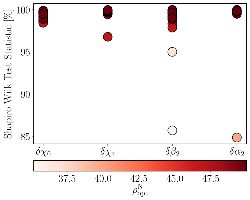
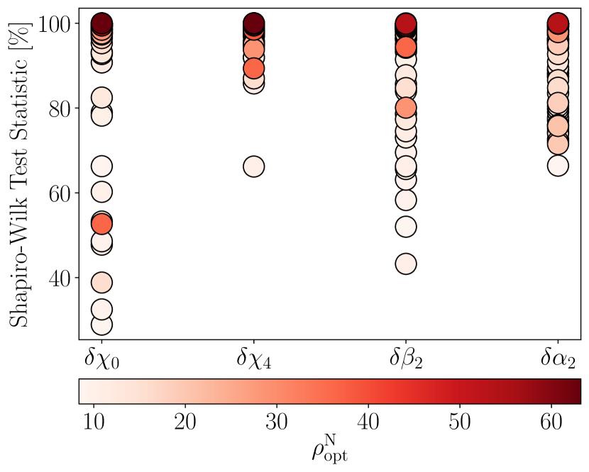
Figure 9: Shapiro-Wilk normality test for the posterior samples of $\{\delta\hat{\chi}_{0}$, $\delta\hat{\chi}_{4}$, $\delta\hat{\alpha}_{2}$, $\delta\hat{\beta}_{2}\}$ in our injections. The colorbar shows the corresponding SNR of the events. Left-panel: Shapiro-Wilk test statistic for samples obtained for GW150914-like injections in Sect. III.1.2 (see also Figs. 4 and 5). Right-panel: Shapiro-Wilk test statistic for the samples obtained for the study of the microlensed population in Sect. III.2.2 (see also Figs. 7 and 8).

Appendix A Normality Test of Posterior Samples

In Sections III.1.2 and III.2.2, we conducted parameterized test analysis using Gaussian sigma values to quantify deviations from General Relativity (GR). However, this approach implicitly assumes that the posterior distributions are Gaussian. To assess the validity of this assumption, we performed the Shapiro-Wilk test of normality Shapiro and Wilk (1965) on our posterior samples of the deviation parameters, namely, $\delta\hat{\chi}_{0}$, $\delta\hat{\chi}_{4}$, $\delta\hat{\alpha}_{2}$, $\delta\hat{\beta}_{2}$. The Shapiro-Wilk test is known to be one of the most powerful normality tests (Mendes and Pala, 2003; Keskin, 2006; Razali et al., 2011). The test statistic, denoted as $\mathcal{SW}$, tends to be higher as the samples more closely resemble a Gaussian distribution and should approach $100\%$ for a true Gaussian distribution.

In Fig. 9, we present the results of the Shapiro-Wilk test. The corresponding SNR values of the events are displayed in the colorbar. The samples obtained for GW150914-like injections in Sect. III.1.2 exhibit a high degree of confidence in being Gaussian distributions. With the exception of two cases, all other cases yield a statistic value above $95\%$ (i.e., $\mathcal{SW}>95\%$ for the majority of cases).

Building on this observation, we introduce a new metric p-index, denoted as $\mathcal{P}$, to quantify the nature of these distributions more robustly. It is defined as the value such that $\mathcal{P}\leavevmode\nobreak\ \%$ of the samples in the distribution have values above $\mathcal{P}\leavevmode\nobreak\ \%$. In mathematical terms, for a distribution $\mathbb{D}=\{d_{i}\}$ of percentages, it can be expressed as:

$$\mathcal{P}=\operatorname*{arg\leavevmode\nobreak\ min}_{x\in(0,100)}\left|\frac{\text{count}(\{d_{i}:d_{i}>x\})}{\text{count}(\{d_{i}\})}-\frac{x}{100}\right|,$$ (19)

where $x$ denotes the possible percentage values, and ‘count’ represents the number of elements in the set inside the parentheses. This additional metric further reinforces our confidence in the Gaussian nature of the data. Specifically, the Shapiro-Wilk test statistic values for our deviation parameters, including $\delta\hat{\chi}_{0}$, $\delta\hat{\chi}_{4}$, $\delta\hat{\alpha}_{2}$, and $\delta\hat{\beta}_{2}$, yield $\mathcal{P}$ values of $98.5\%,\leavevmode\nobreak\ 96.8\%,\leavevmode\nobreak\ 95.0\%,$ and $96.7\%$, respectively. For instance, this means that the statistic values for the posterior distribution of $\delta\hat{\chi}_{0}$ are above $98.5\%$ for approximately $98.5\%$ of the cases, and so on.

In a similar fashion, the right-panel of Fig. 9 displays the test statistic results for the samples obtained during the study of the microlensed population in Sect. III.2.2. Here, $\mathcal{P}$ values for our deviation parameters, $\delta\hat{\chi}_{0}$, $\delta\hat{\chi}_{4}$, $\delta\hat{\alpha}_{2}$, and $\delta\hat{\beta}_{2}$ are $88.0\%,\leavevmode\nobreak\ 93.8\%,\leavevmode\nobreak\ 84.7\%,$ and $82.7\%$, respectively.

In conclusion, the assumption of Gaussianity holds well in our case, especially for high SNR events. For GW150914-like injections, approximately $95\%$ of the cases yielded a statistic value exceeding $95\%$, while in the case of the population study, approximately $85\%$ of the cases yielded a statistic value above $85\%$.

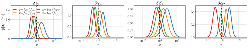
Figure 10: Gaussian fits to the distribution of $\sigma_{\mathrm{GR}}$ for the microlensed population injections plotted against the variable $x\in\{f_{\mathrm{ML}}/f_{\mathrm{low}},\leavevmode\nobreak\ f_{\mathrm{ML}}/f_{\mathrm{avg.}},\leavevmode\nobreak\ f_{\mathrm{ML}}/f_{\mathrm{ISCO}},\leavevmode\nobreak\ f_{\mathrm{ML}}/f_{\mathrm{RD}}\}$ for all the deviation parameters $\{\delta\hat{\chi}_{0},\leavevmode\nobreak\ \delta\hat{\chi}_{4},\leavevmode\nobreak\ \delta\hat{\alpha}_{2},\leavevmode\nobreak\ \delta\hat{\beta}_{2}\}$ (indicated on top of each panel). A dashed-black line is included at $x=1$ for reference, representing the characteristic frequency of GW $f_{\mathrm{GW}}^{\mathrm{c}}$ which when comparable to $f_{\mathrm{ML}}$ gives rise to wave effects.

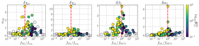
Figure 11: The distribution of $\sigma_{\mathrm{GR}}$ is analyzed in the context of some selected values of $x$ for different deviation parameters. Leftmost two panels: $x=f_{\mathrm{ML}}/f_{\mathrm{avg.}}$ is considered with deviation parameters $\{\delta\hat{\chi}_{0},\delta\hat{\chi}_{4}\}$. Rightmost two panels: For parameters $\{\delta\hat{\alpha}_{2},\delta\hat{\beta}_{2}\}$, we choose $x=f_{\mathrm{ML}}/f_{\mathrm{ISCO}}$. A dashed-red line at $x=1$ is included for reference.

Appendix B Investigating the correspondence between $f_{\mathrm{ML}}$ and $f_{\mathrm{GW}}$: A closer perspective

As discussed in Section II.1, the condition for wave effects is that $f_{\mathrm{ML}}\sim f_{\mathrm{GW}}$. In the sections leading up to this point, we assumed that $f_{\mathrm{GW}}\in(10,1000)$ Hz, based on the sensitivity of ground-based detectors. However, we can be more precise in defining the characteristic frequency of GW, denoted as $f_{\mathrm{GW}}^{\mathrm{c}}$, which when comparable to $f_{\mathrm{ML}}$ gives rise to wave effects. This approach is possible because, for a given GW signal, we can explicitly determine the frequency range where it exhibits significant power in the detectors. Therefore, in this section, we leverage this knowledge to establish a closer correspondence between $f_{\mathrm{ML}}$ and $f_{\mathrm{GW}}$.

The lower frequency cutoff typically used for GW data analysis is $f_{\mathrm{low}}=20\leavevmode\nobreak\$Hz, below which the noise dramatically increases, especially due to seismic and thermal noise sources (Abbott et al., 2016b; Valdes et al., 2022). Next, the inspiral and post-inspiral sections are typically demarcated using the frequency at the inner-most stable circular orbit $f_{\mathrm{ISCO}}$ (Hanna et al., 2009; Abbott et al., 2021e), which is the same cutoff frequency we used for IMRCT (see Sect. II.2.1). We note that this demarcation is not the same as the demarcation used for the parameterized test. Moreover, a rough estimate of the upper frequency of a GW signal can be determined based on the ringdown frequency, $f_{\mathrm{RD}}$, associated with the dominant quasi-normal mode $(l=2,\leavevmode\nobreak\ m=2,\leavevmode\nobreak\ n=0)$ (Hanna et al., 2009; Berti et al., 2006). Additionally, one can define a signal’s power-weighted average frequency, denoted as $f_{\mathrm{avg.}}$, using the following equation:

$$f_{\mathrm{avg.}}=\frac{\int_{-\infty}^{\infty}f\cdot|\widetilde{h}(f)|^{2}df}{\int_{-\infty}^{\infty}|\widetilde{h}(f)|^{2}df}.$$ (20)

This power-weighted average frequency reflects where most of the signal power is concentrated. In the case of GW signals, the inspiral phase typically contributes the most power. Consequently, we usually expect $f_{\mathrm{avg.}}<f_{\mathrm{ISCO}}$. Thus, a signal that spans a sufficient number of cycles in the inspiral phase within the current detectors can be effectively divided into different phases of its evolution using these frequency markers: $f_{\mathrm{low}}<f_{\mathrm{avg.}}<f_{\mathrm{ISCO}}<f_{\mathrm{RD}}$.

We consider posterior distributions of the deviation parameters, namely, $\delta\hat{\chi}_{0}$, $\delta\hat{\chi}_{4}$, $\delta\hat{\alpha}_{2}$, and $\delta\hat{\beta}_{2}$, for the different injections studied in III.2.2. Since the characteristic frequencies mentioned above differ for each injection, we study the ratio of $f_{\mathrm{ML}}$ with these frequencies, i.e., we examine the quantity: $x:x\in\{f_{\mathrm{ML}}/f_{\mathrm{low}},\leavevmode\nobreak\ f_{\mathrm{ML}}/f_{\mathrm{avg.}},\leavevmode\nobreak\ f_{\mathrm{ML}}/f_{\mathrm{ISCO}},\leavevmode\nobreak\ f_{\mathrm{ML}}/f_{\mathrm{RD}}\}$. Given that the condition for pronounced wave effects is $f_{\mathrm{ML}}\sim f_{\mathrm{GW}}^{\mathrm{c}}$, we analyze the distribution of $\sigma_{\mathrm{GR}}$ as a function of $x$ to determine which ratio results in a peak near $1$.

In Fig. 10, we present the distribution of $\sigma_{\mathrm{GR}}$ for the microlensed population injections against the variable $x$ for all the deviation parameters (indicated on top of each panel). To enhance clarity, we employ Gaussian fits to combine all four $\sigma_{\mathrm{GR}}-x$ distributions of a given deviation parameter into a single panel. An example illustrating the actual $\sigma_{\mathrm{GR}}-x$ distribution is provided in Fig. 11 for specific cases. We also include a dashed-black reference line at $x=1$, representing the frequency where $f_{\mathrm{ML}}\sim f_{\mathrm{GW}}^{\mathrm{c}}$. Given that, for our injections, $1/f_{\mathrm{RD}}<1/f_{\mathrm{ISCO}}<1/f_{\mathrm{avg.}}<1/f_{\mathrm{low}}$, the Gaussian curves follow a consistent trend. Specifically, the $\sigma_{\mathrm{GR}}-x$ distribution for $x=f_{\mathrm{ML}}/f_{\mathrm{RD}}$ occupies the leftmost position with its peak significantly below 1 (indicated by the red curves), while for $x=f_{\mathrm{ML}}/f_{\mathrm{low}}$, it occupies the rightmost position in all panels with the peak significantly above 1 (indicated by the blue curves). In other words, assuming $f_{\mathrm{GW}}^{\mathrm{c}}=f_{\mathrm{low}}$ would result in an underestimation, whereas assuming $f_{\mathrm{GW}}^{\mathrm{c}}=f_{\mathrm{RD}}$ would lead to an overestimation. Therefore, the fact that the curves of these ratios lie on different sides of unity implies that the condition for microlensing in the case of a given GW signal can be more precisely defined as when $f_{\mathrm{ML}}\in(f_{\mathrm{low}},\leavevmode\nobreak\ f_{\mathrm{RD}})$, as opposed to the generic range of $(10,\leavevmode\nobreak\ 1000)$Hz we used earlier.

We also note that for the deviation parameters $\delta\hat{\chi}_{0}$ and $\delta\hat{\chi}_{4}$, the peak corresponding to $x=f_{\mathrm{ML}}/f_{\mathrm{avg.}}$ is closest to unity. This implies that these deviation parameters exhibit the highest bias when $f_{\mathrm{ML}}\sim f_{\mathrm{GW}}^{\mathrm{c}}\sim f_{\mathrm{avg.}}$. This outcome is expected because these parameters primarily measure deviations from GR during the inspiral phase of the signal. In Fig. 11, we explicitly depict the distribution of $\sigma_{\mathrm{GR}}$ for the $x=f_{\mathrm{ML}}/f_{\mathrm{avg.}}$ ratio for these two parameters in the leftmost two columns, where we observe an increase in deviations around $x\sim 1$. In contrast, for the deviation parameters $\delta\hat{\alpha}_{2}$ and $\delta\hat{\beta}_{2}$, the peak corresponding to $x=f_{\mathrm{ML}}/f_{\mathrm{ISCO}}$ is closest to unity, indicating that these deviation parameters exhibit the highest bias when $f_{\mathrm{ML}}\sim f_{\mathrm{GW}}^{\mathrm{c}}\sim f_{\mathrm{ISCO}}$. This can be explained by the fact that these parameters primarily measure deviations from GR during the post-inspiral phase of the signal. In Fig. 11, we explicitly display the distribution of $\sigma_{\mathrm{GR}}$ for the $x=f_{\mathrm{ML}}/f_{\mathrm{ISCO}}$ ratio for these two parameters in the rightmost two columns, where, once again, we notice an increase in deviations around $x\sim 1$.

In conclusion, we find that the condition for microlensing in the case of a given GW signal can be more precisely defined as when $f_{\mathrm{ML}}\in(f_{\mathrm{low}},\leavevmode\nobreak\ f_{\mathrm{RD}})$, as opposed to the generic range of $(10,\leavevmode\nobreak\ 1000)\leavevmode\nobreak\$Hz we used earlier. We went further and tried to find even specific conditions. For example, for parameters that measure deviations in the inspiral regime, such as $\delta\hat{\chi}_{0}$ and $\delta\hat{\chi}_{4}$, the deviations increase when $f_{\mathrm{ML}}\sim f_{\mathrm{avg.}}$. While for parameters that measure deviations in the post-inspiral regime, such as $\delta\hat{\alpha}_{2}$ and $\delta\hat{\beta}_{2}$, the deviations increase when $f_{\mathrm{ML}}\sim f_{\mathrm{ISCO}}$.

Appendix C Additional Figures

References

- Will (2014) Clifford M. Will, “The Confrontation between General Relativity and Experiment,” Living Rev. Rel. 17, 4 (2014), arXiv:1403.7377 [gr-qc] .
- Wex (2014) Norbert Wex, “Testing Relativistic Gravity with Radio Pulsars,” (2014), arXiv:1402.5594 [gr-qc] .
- Aasi et al. (2015) J. Aasi et al. (LIGO Scientific), “Advanced LIGO,” Class. Quant. Grav. 32, 074001 (2015), arXiv:1411.4547 [gr-qc] .
- Acernese et al. (2015) F. Acernese et al. (VIRGO), “Advanced Virgo: a second-generation interferometric gravitational wave detector,” Class. Quant. Grav. 32, 024001 (2015), arXiv:1408.3978 [gr-qc] .
- Abbott et al. (2019a) B. P. Abbott et al. (LIGO Scientific, Virgo), “GWTC-1: A Gravitational-Wave Transient Catalog of Compact Binary Mergers Observed by LIGO and Virgo during the First and Second Observing Runs,” Phys. Rev. X 9, 031040 (2019a), arXiv:1811.12907 [astro-ph.HE] .
- Abbott et al. (2021a) R. Abbott et al. (LIGO Scientific, Virgo), “GWTC-2: Compact Binary Coalescences Observed by LIGO and Virgo During the First Half of the Third Observing Run,” Phys. Rev. X 11, 021053 (2021a), arXiv:2010.14527 [gr-qc] .
- Abbott et al. (2021b) R. Abbott et al. (LIGO Scientific, VIRGO), “GWTC-2.1: Deep Extended Catalog of Compact Binary Coalescences Observed by LIGO and Virgo During the First Half of the Third Observing Run,” (2021b), arXiv:2108.01045 [gr-qc] .
- Abbott et al. (2021c) R. Abbott et al. (LIGO Scientific, VIRGO, KAGRA), “GWTC-3: Compact Binary Coalescences Observed by LIGO and Virgo During the Second Part of the Third Observing Run,” (2021c), arXiv:2111.03606 [gr-qc] .
- Abbott et al. (2016a) B. P. Abbott et al. (LIGO Scientific, Virgo), “Tests of general relativity with GW150914,” Phys. Rev. Lett. 116, 221101 (2016a), [Erratum: Phys.Rev.Lett. 121, 129902 (2018)], arXiv:1602.03841 [gr-qc] .
- Abbott et al. (2019b) B. P. Abbott et al. (LIGO Scientific, Virgo), “Tests of General Relativity with GW170817,” Phys. Rev. Lett. 123, 011102 (2019b), arXiv:1811.00364 [gr-qc] .
- Abbott et al. (2019c) B. P. Abbott et al. (LIGO Scientific, Virgo), “Tests of General Relativity with the Binary Black Hole Signals from the LIGO-Virgo Catalog GWTC-1,” Phys. Rev. D 100, 104036 (2019c), arXiv:1903.04467 [gr-qc] .
- Abbott et al. (2021d) R. Abbott et al. (LIGO Scientific, Virgo), “Tests of general relativity with binary black holes from the second LIGO-Virgo gravitational-wave transient catalog,” Phys. Rev. D 103, 122002 (2021d), arXiv:2010.14529 [gr-qc] .
- Abbott et al. (2021e) R. Abbott et al. (LIGO Scientific, VIRGO, KAGRA), “Tests of General Relativity with GWTC-3,” (2021e), arXiv:2112.06861 [gr-qc] .
- Collett and Bacon (2017) Thomas E. Collett and David Bacon, “Testing the speed of gravitational waves over cosmological distances with strong gravitational lensing,” Phys. Rev. Lett. 118, 091101 (2017), arXiv:1602.05882 [astro-ph.HE] .
- Fan et al. (2017) Xi-Long Fan, Kai Liao, Marek Biesiada, Aleksandra Piorkowska-Kurpas, and Zong-Hong Zhu, “Speed of Gravitational Waves from Strongly Lensed Gravitational Waves and Electromagnetic Signals,” Phys. Rev. Lett. 118, 091102 (2017), arXiv:1612.04095 [gr-qc] .
- Yang et al. (2019) Tao Yang, Bin Hu, Rong-Gen Cai, and Bin Wang, “New probe of gravity: strongly lensed gravitational wave multi-messenger approach,” Astrophys. J. 880, 50 (2019), arXiv:1810.00164 [astro-ph.CO] .
- Chung and Li (2021) Adrian Ka-Wai Chung and Tjonnie Guang Feng Li, “Lensing of gravitational waves as a novel probe of graviton mass,” Phys. Rev. D 104, 124060 (2021), arXiv:2106.09630 [gr-qc] .
- Mukherjee et al. (2020a) Suvodip Mukherjee, Benjamin D. Wandelt, and Joseph Silk, “Probing the theory of gravity with gravitational lensing of gravitational waves and galaxy surveys,” Mon. Not. Roy. Astron. Soc. 494, 1956–1970 (2020a), arXiv:1908.08951 [astro-ph.CO] .
- Mukherjee et al. (2020b) Suvodip Mukherjee, Benjamin D. Wandelt, and Joseph Silk, “Multimessenger tests of gravity with weakly lensed gravitational waves,” Phys. Rev. D 101, 103509 (2020b), arXiv:1908.08950 [astro-ph.CO] .
- Finke et al. (2021) Andreas Finke, Stefano Foffa, Francesco Iacovelli, Michele Maggiore, and Michele Mancarella, “Probing modified gravitational wave propagation with strongly lensed coalescing binaries,” Phys. Rev. D 104, 084057 (2021), arXiv:2107.05046 [gr-qc] .
- Iacovelli et al. (2022) Francesco Iacovelli, Andreas Finke, Stefano Foffa, Michele Maggiore, and Michele Mancarella, “Modified gravitational wave propagation: information from strongly lensed binaries and the BNS mass function,” in 56th Rencontres de Moriond on Gravitation (2022) arXiv:2203.09237 [gr-qc] .
- Goyal et al. (2021) Srashti Goyal, K. Haris, Ajit Kumar Mehta, and Parameswaran Ajith, “Testing the nature of gravitational-wave polarizations using strongly lensed signals,” Phys. Rev. D 103, 024038 (2021), arXiv:2008.07060 [gr-qc] .
- Magaña Hernandez (2022) Ignacio Magaña Hernandez, “Measuring the polarization content of gravitational waves with strongly lensed binary black hole mergers,” (2022), arXiv:2211.01272 [gr-qc] .
- Goyal et al. (2023) Srashti Goyal, Aditya Vijaykumar, Jose Maria Ezquiaga, and Miguel Zumalacarregui, “Probing lens-induced gravitational-wave birefringence as a test of general relativity,” Phys. Rev. D 108, 024052 (2023), arXiv:2301.04826 [gr-qc] .
- Liu et al. (2023) Anna Liu, Isaac C. F. Wong, Samson H. W. Leong, Anupreeta More, Otto A. Hannuksela, and Tjonnie G. F. Li, “Exploring the hidden Universe: a novel phenomenological approach for recovering arbitrary gravitational-wave millilensing configurations,” Mon. Not. Roy. Astron. Soc. 525, 4149–4160 (2023), arXiv:2302.09870 [gr-qc] .
- Janquart et al. (2023) Justin Janquart et al., “Follow-up Analyses to the O3 LIGO-Virgo-KAGRA Lensing Searches,” (2023), 10.1093/mnras/stad2909, arXiv:2306.03827 [gr-qc] .
- Deguchi and Watson (1986) S. Deguchi and W. D. Watson, “Diffraction in Gravitational Lensing for Compact Objects of Low Mass,” Astrophys. J. 307, 30 (1986).
- Nakamura (1998) Takahiro T. Nakamura, “Gravitational lensing of gravitational waves from inspiraling binaries by a point mass lens,” Phys. Rev. Lett. 80, 1138–1141 (1998).
- Baraldo et al. (1999) Christian Baraldo, Akio Hosoya, and Takahiro T. Nakamura, “Gravitationally induced interference of gravitational waves by a rotating massive object,” Phys. Rev. D 59, 083001 (1999).
- Nakamura and Deguchi (1999) Takahiro T. Nakamura and Shuji Deguchi, “Wave Optics in Gravitational Lensing,” Prog. Theor. Phys. Suppl. 133, 137–153 (1999).
- Bulashenko and Ubach (2022) Oleg Bulashenko and Helena Ubach, “Lensing of gravitational waves: universal signatures in the beating pattern,” JCAP 07, 022 (2022), arXiv:2112.10773 [gr-qc] .
- Leung et al. (2023) Calvin Leung, Dylan Jow, Prasenjit Saha, Liang Dai, Masamune Oguri, and Léon V. E. Koopmans, “Wave Mechanics, Interference, and Decoherence in Strong Gravitational Lensing,” (2023), arXiv:2304.01202 [astro-ph.HE] .
- Mishra et al. (2023) Anuj Mishra, Ashish Kumar Meena, Anupreeta More, and Sukanta Bose, “Exploring the impact of microlensing on gravitational wave signals: Biases, population characteristics, and prospects for detection,” arXiv preprint arXiv:2306.11479 (2023).
- Abbott et al. (2021f) R. Abbott et al. (LIGO Scientific, VIRGO), “Search for Lensing Signatures in the Gravitational-Wave Observations from the First Half of LIGO–Virgo’s Third Observing Run,” Astrophys. J. 923, 14 (2021f), arXiv:2105.06384 [gr-qc] .
- Abbott et al. (2023) R. Abbott et al. (LIGO Scientific, VIRGO, KAGRA), “Search for gravitational-lensing signatures in the full third observing run of the LIGO-Virgo network,” (2023), arXiv:2304.08393 [gr-qc] .
- Jung and Shin (2019) Sunghoon Jung and Chang Sub Shin, “Gravitational-Wave Fringes at LIGO: Detecting Compact Dark Matter by Gravitational Lensing,” Phys. Rev. Lett. 122, 041103 (2019), arXiv:1712.01396 [astro-ph.CO] .
- Basak et al. (2022) S. Basak, A. Ganguly, K. Haris, S. Kapadia, A. K. Mehta, and P. Ajith, “Constraints on Compact Dark Matter from Gravitational Wave Microlensing,” Astrophys. J. 926, L28 (2022), arXiv:2109.06456 [gr-qc] .
- Diego (2020) Jose M. Diego, “Constraining the abundance of primordial black holes with gravitational lensing of gravitational waves at LIGO frequencies,” Phys. Rev. D 101, 123512 (2020), arXiv:1911.05736 [astro-ph.CO] .
- Diego et al. (2019) J. M. Diego, O. A. Hannuksela, P. L. Kelly, T. Broadhurst, K. Kim, T. G. F. Li, G. F. Smoot, and G. Pagano, “Observational signatures of microlensing in gravitational waves at LIGO/Virgo frequencies,” Astron. Astrophys. 627, A130 (2019), arXiv:1903.04513 [astro-ph.CO] .
- Seo et al. (2021) Eungwang Seo, Otto A. Hannuksela, and Tjonnie G. F. Li, “Strong lensing: A magnifying glass to detect gravitational-wave microlensing,” in 17th International Conference on Topics in Astroparticle and Underground Physics (2021) arXiv:2110.03308 [astro-ph.HE] .
- Mishra et al. (2021) Anuj Mishra, Ashish Kumar Meena, Anupreeta More, Sukanta Bose, and Jasjeet Singh Bagla, “Gravitational lensing of gravitational waves: effect of microlens population in lensing galaxies,” Mon. Not. Roy. Astron. Soc. 508, 4869–4886 (2021), arXiv:2102.03946 [astro-ph.CO] .
- Meena et al. (2022) Ashish Kumar Meena, Anuj Mishra, Anupreeta More, Sukanta Bose, and Jasjeet Singh Bagla, “Gravitational lensing of gravitational waves: Probability of microlensing in galaxy-scale lens population,” Mon. Not. Roy. Astron. Soc. 517, 872–884 (2022), arXiv:2205.05409 [astro-ph.GA] .
- Meena (2023) Ashish Kumar Meena, “Gravitational Lensing of Gravitational Waves: Probing Intermediate Mass Black Holes in Galaxy Lenses with Global Minima,” (2023), arXiv:2305.02880 [astro-ph.CO] .
- Çalışkan et al. (2023a) Mesut Çalışkan, Lingyuan Ji, Roberto Cotesta, Emanuele Berti, Marc Kamionkowski, and Sylvain Marsat, “Observability of lensing of gravitational waves from massive black hole binaries with LISA,” Phys. Rev. D 107, 043029 (2023a), arXiv:2206.02803 [astro-ph.CO] .
- Çalışkan et al. (2023b) Mesut Çalışkan, Neha Anil Kumar, Lingyuan Ji, Jose M. Ezquiaga, Roberto Cotesta, Emanuele Berti, and Marc Kamionkowski, “Probing wave-optics effects and dark-matter subhalos with lensing of gravitational waves from massive black holes,” (2023b), arXiv:2307.06990 [astro-ph.CO] .
- Ghosh et al. (2016) Abhirup Ghosh et al., “Testing general relativity using golden black-hole binaries,” Phys. Rev. D 94, 021101 (2016), arXiv:1602.02453 [gr-qc] .
- Ghosh et al. (2018) Abhirup Ghosh, Nathan K. Johnson-Mcdaniel, Archisman Ghosh, Chandra Kant Mishra, Parameswaran Ajith, Walter Del Pozzo, Christopher P. L. Berry, Alex B. Nielsen, and Lionel London, “Testing general relativity using gravitational wave signals from the inspiral, merger and ringdown of binary black holes,” Class. Quant. Grav. 35, 014002 (2018), arXiv:1704.06784 [gr-qc] .
- Arun et al. (2006a) K. G. Arun, Bala R. Iyer, M. S. S. Qusailah, and B. S. Sathyaprakash, “Testing post-Newtonian theory with gravitational wave observations,” Class. Quant. Grav. 23, L37–L43 (2006a), arXiv:gr-qc/0604018 .
- Arun et al. (2006b) K. G. Arun, Bala R. Iyer, M. S. S. Qusailah, and B. S. Sathyaprakash, “Probing the non-linear structure of general relativity with black hole binaries,” Phys. Rev. D 74, 024006 (2006b), arXiv:gr-qc/0604067 .
- Yunes and Pretorius (2009) Nicolas Yunes and Frans Pretorius, “Fundamental Theoretical Bias in Gravitational Wave Astrophysics and the Parameterized Post-Einsteinian Framework,” Phys. Rev. D 80, 122003 (2009), arXiv:0909.3328 [gr-qc] .
- Li et al. (2012) T. G. F. Li, W. Del Pozzo, S. Vitale, C. Van Den Broeck, M. Agathos, J. Veitch, K. Grover, T. Sidery, R. Sturani, and A. Vecchio, “Towards a generic test of the strong field dynamics of general relativity using compact binary coalescence,” Phys. Rev. D 85, 082003 (2012), arXiv:1110.0530 [gr-qc] .
- Yunes et al. (2016) Nicolas Yunes, Kent Yagi, and Frans Pretorius, “Theoretical Physics Implications of the Binary Black-Hole Mergers GW150914 and GW151226,” Phys. Rev. D 94, 084002 (2016), arXiv:1603.08955 [gr-qc] .
- Ezquiaga et al. (2022) Jose Maria Ezquiaga, Wayne Hu, Macarena Lagos, Meng-Xiang Lin, and Fei Xu, “Modified gravitational wave propagation with higher modes and its degeneracies with lensing,” JCAP 08, 016 (2022), arXiv:2203.13252 [gr-qc] .
- Janquart et al. (2021) Justin Janquart, Eungwang Seo, Otto A. Hannuksela, Tjonnie G. F. Li, and Chris Van Den Broeck, “On the Identification of Individual Gravitational-wave Image Types of a Lensed System Using Higher-order Modes,” Astrophys. J. Lett. 923, L1 (2021), arXiv:2110.06873 [gr-qc] .
- Vijaykumar et al. (2023) Aditya Vijaykumar, Ajit Kumar Mehta, and Apratim Ganguly, “Detection and parameter estimation challenges of type-II lensed binary black hole signals,” Phys. Rev. D 108, 043036 (2023), arXiv:2202.06334 [gr-qc] .
- Mollerach and Roulet (2002) Silvia Mollerach and Esteban Roulet, Gravitational lensing and microlensing (World Scientific, 2002).
- Schneider et al. (1992) Peter Schneider, Jürgen Ehlers, and Emilio E. Falco, Gravitational Lenses (Springer, Berlin, Heidelberg, 1992).
- Oguri (2018) Masamune Oguri, “Effect of gravitational lensing on the distribution of gravitational waves from distant binary black hole mergers,” Mon. Not. Roy. Astron. Soc. 480, 3842–3855 (2018), arXiv:1807.02584 [astro-ph.CO] .
- More and More (2022) Anupreeta More and Surhud More, “Improved statistic to identify strongly lensed gravitational wave events,” Mon. Not. Roy. Astron. Soc. 515, 1044–1051 (2022), arXiv:2111.03091 [astro-ph.CO] .
- Hannuksela et al. (2019) O. A. Hannuksela, K. Haris, K. K. Y. Ng, S. Kumar, A. K. Mehta, D. Keitel, T. G. F. Li, and P. Ajith, “Search for gravitational lensing signatures in LIGO-Virgo binary black hole events,” Astrophys. J. Lett. 874, L2 (2019), arXiv:1901.02674 [gr-qc] .
- Dai et al. (2020) Liang Dai, Barak Zackay, Tejaswi Venumadhav, Javier Roulet, and Matias Zaldarriaga, “Search for Lensed Gravitational Waves Including Morse Phase Information: An Intriguing Candidate in O2,” (2020), arXiv:2007.12709 [astro-ph.HE] .
- Dai and Venumadhav (2017) Liang Dai and Tejaswi Venumadhav, “On the waveforms of gravitationally lensed gravitational waves,” (2017), arXiv:1702.04724 [gr-qc] .
- Takahashi and Nakamura (2003) Ryuichi Takahashi and Takashi Nakamura, “Wave effects in gravitational lensing of gravitational waves from chirping binaries,” Astrophys. J. 595, 1039–1051 (2003), arXiv:astro-ph/0305055 .
- Goodman (2005) Joseph W Goodman, Introduction to Fourier optics (Roberts and Company Publishers, 2005).
- Schneider and Weiss (1986) Peter Schneider and Achim Weiss, “The two-point-mass lens-detailed investigation of a special asymmetric gravitational lens,” Astronomy and Astrophysics 164, 237–259 (1986).
- Bondarescu et al. (2023) Ruxandra Bondarescu, Helena Ubach, Oleg Bulashenko, and Andrew P. Lundgren, “Compact binaries through a lens: Silent versus detectable microlensing for the LIGO-Virgo-KAGRA gravitational wave observatories,” Phys. Rev. D 108, 084033 (2023), arXiv:2211.13604 [gr-qc] .
- Tambalo et al. (2023) Giovanni Tambalo, Miguel Zumalacárregui, Liang Dai, and Mark Ho-Yeuk Cheung, “Lensing of gravitational waves: Efficient wave-optics methods and validation with symmetric lenses,” Phys. Rev. D 108, 043527 (2023), arXiv:2210.05658 [gr-qc] .
- Narayan et al. (2023) Purnima Narayan, Nathan K. Johnson-McDaniel, and Anuradha Gupta, “Effect of ignoring eccentricity in testing general relativity with gravitational waves,” Phys. Rev. D 108, 064003 (2023), arXiv:2306.04068 [gr-qc] .
- Saini et al. (2022) Pankaj Saini, Marc Favata, and K. G. Arun, “Systematic bias on parametrized tests of general relativity due to neglect of orbital eccentricity,” Phys. Rev. D 106, 084031 (2022), arXiv:2203.04634 [gr-qc] .
- Bhat et al. (2023) Sajad A. Bhat, Pankaj Saini, Marc Favata, and K. G. Arun, “Systematic bias on the inspiral-merger-ringdown consistency test due to neglect of orbital eccentricity,” Phys. Rev. D 107, 024009 (2023), arXiv:2207.13761 [gr-qc] .
- Abbott et al. (2017) Benjamin P. Abbott et al. (LIGO Scientific, VIRGO), “GW170104: Observation of a 50-Solar-Mass Binary Black Hole Coalescence at Redshift 0.2,” Phys. Rev. Lett. 118, 221101 (2017), [Erratum: Phys.Rev.Lett. 121, 129901 (2018)], arXiv:1706.01812 [gr-qc] .
- (72) Nathan K. Johnson-McDaniel et al., “Determining the final spin of a binary black hole system including in-plane spins: Method and checks of accuracy,” .
- Hofmann et al. (2016) Fabian Hofmann, Enrico Barausse, and Luciano Rezzolla, “The final spin from binary black holes in quasi-circular orbits,” Astrophys. J. Lett. 825, L19 (2016), arXiv:1605.01938 [gr-qc] .
- Jiménez-Forteza et al. (2017) Xisco Jiménez-Forteza, David Keitel, Sascha Husa, Mark Hannam, Sebastian Khan, and Michael Pürrer, “Hierarchical data-driven approach to fitting numerical relativity data for nonprecessing binary black holes with an application to final spin and radiated energy,” Phys. Rev. D 95, 064024 (2017), arXiv:1611.00332 [gr-qc] .
- Healy and Lousto (2017) James Healy and Carlos O. Lousto, “Remnant of binary black-hole mergers: New simulations and peak luminosity studies,” Phys. Rev. D 95, 024037 (2017), arXiv:1610.09713 [gr-qc] .
- Hoy and Raymond (2021) Charlie Hoy and Vivien Raymond, “PESummary: the code agnostic Parameter Estimation Summary page builder,” SoftwareX 15, 100765 (2021), arXiv:2006.06639 [astro-ph.IM] .
- Pratten et al. (2021) Geraint Pratten et al., “Computationally efficient models for the dominant and subdominant harmonic modes of precessing binary black holes,” Phys. Rev. D 103, 104056 (2021), arXiv:2004.06503 [gr-qc] .
- Blanchet (2014) Luc Blanchet, “Gravitational Radiation from Post-Newtonian Sources and Inspiralling Compact Binaries,” Living Rev. Rel. 17, 2 (2014), arXiv:1310.1528 [gr-qc] .
- Pretorius (2007) Frans Pretorius, “Binary Black Hole Coalescence,” (2007), arXiv:0710.1338 [gr-qc] .
- Duez and Zlochower (2019) Matthew D. Duez and Yosef Zlochower, “Numerical Relativity of Compact Binaries in the 21st Century,” Rept. Prog. Phys. 82, 016902 (2019), arXiv:1808.06011 [gr-qc] .
- Berti et al. (2006) Emanuele Berti, Vitor Cardoso, and Clifford M. Will, “On gravitational-wave spectroscopy of massive black holes with the space interferometer LISA,” Phys. Rev. D 73, 064030 (2006), arXiv:gr-qc/0512160 .
- Agathos et al. (2014) Michalis Agathos, Walter Del Pozzo, Tjonnie G. F. Li, Chris Van Den Broeck, John Veitch, and Salvatore Vitale, “TIGER: A data analysis pipeline for testing the strong-field dynamics of general relativity with gravitational wave signals from coalescing compact binaries,” Phys. Rev. D 89, 082001 (2014), arXiv:1311.0420 [gr-qc] .
- Meidam et al. (2018) Jeroen Meidam et al., “Parametrized tests of the strong-field dynamics of general relativity using gravitational wave signals from coalescing binary black holes: Fast likelihood calculations and sensitivity of the method,” Phys. Rev. D 97, 044033 (2018), arXiv:1712.08772 [gr-qc] .
- Ajith et al. (2008) P. Ajith et al., “A Template bank for gravitational waveforms from coalescing binary black holes. I. Non-spinning binaries,” Phys. Rev. D 77, 104017 (2008), [Erratum: Phys.Rev.D 79, 129901 (2009)], arXiv:0710.2335 [gr-qc] .
- Ajith et al. (2011) P. Ajith et al., “Inspiral-merger-ringdown waveforms for black-hole binaries with non-precessing spins,” Phys. Rev. Lett. 106, 241101 (2011), arXiv:0909.2867 [gr-qc] .
- Santamaria et al. (2010) L. Santamaria et al., “Matching post-Newtonian and numerical relativity waveforms: systematic errors and a new phenomenological model for non-precessing black hole binaries,” Phys. Rev. D 82, 064016 (2010), arXiv:1005.3306 [gr-qc] .
- Husa et al. (2016) Sascha Husa, Sebastian Khan, Mark Hannam, Michael Pürrer, Frank Ohme, Xisco Jiménez Forteza, and Alejandro Bohé, “Frequency-domain gravitational waves from nonprecessing black-hole binaries. I. New numerical waveforms and anatomy of the signal,” Phys. Rev. D 93, 044006 (2016), arXiv:1508.07250 [gr-qc] .
- Khan et al. (2016) Sebastian Khan, Sascha Husa, Mark Hannam, Frank Ohme, Michael Pürrer, Xisco Jiménez Forteza, and Alejandro Bohé, “Frequency-domain gravitational waves from nonprecessing black-hole binaries. II. A phenomenological model for the advanced detector era,” Phys. Rev. D 93, 044007 (2016), arXiv:1508.07253 [gr-qc] .
- García-Quirós et al. (2020) Cecilio García-Quirós, Marta Colleoni, Sascha Husa, Héctor Estellés, Geraint Pratten, Antoni Ramos-Buades, Maite Mateu-Lucena, and Rafel Jaume, “Multimode frequency-domain model for the gravitational wave signal from nonprecessing black-hole binaries,” Phys. Rev. D 102, 064002 (2020), arXiv:2001.10914 [gr-qc] .
- Pratten et al. (2020) Geraint Pratten, Sascha Husa, Cecilio Garcia-Quiros, Marta Colleoni, Antoni Ramos-Buades, Hector Estelles, and Rafel Jaume, “Setting the cornerstone for a family of models for gravitational waves from compact binaries: The dominant harmonic for nonprecessing quasicircular black holes,” Phys. Rev. D 102, 064001 (2020), arXiv:2001.11412 [gr-qc] .
- Hannam et al. (2014) Mark Hannam, Patricia Schmidt, Alejandro Bohé, Leïla Haegel, Sascha Husa, Frank Ohme, Geraint Pratten, and Michael Pürrer, “Simple Model of Complete Precessing Black-Hole-Binary Gravitational Waveforms,” Phys. Rev. Lett. 113, 151101 (2014), arXiv:1308.3271 [gr-qc] .
- (92) Bohe Alejandro et al., “PhenomPv2 – technical notes for the LAL implementation,” .
- Abbott et al. (2020) Benjamin P Abbott, R Abbott, TD Abbott, S Abraham, F Acernese, K Ackley, C Adams, VB Adya, C Affeldt, M Agathos, et al., “Prospects for observing and localizing gravitational-wave transients with advanced ligo, advanced virgo and kagra,” Living reviews in relativity 23, 1–69 (2020).
- Pürrer et al. (2017) Michael Pürrer, Mark Hannam, and Frank Ohme, “Can we measure individual black-hole spins from gravitational-wave observations?” in 14th Marcel Grossmann Meeting on Recent Developments in Theoretical and Experimental General Relativity, Astrophysics, and Relativistic Field Theories, Vol. 3 (2017) pp. 3144–3148.
- Madau and Dickinson (2014) Piero Madau and Mark Dickinson, “Cosmic Star Formation History,” Ann. Rev. Astron. Astrophys. 52, 415–486 (2014), arXiv:1403.0007 [astro-ph.CO] .
- Fishbach et al. (2018) Maya Fishbach, Daniel E. Holz, and Will M. Farr, “Does the Black Hole Merger Rate Evolve with Redshift?” Astrophys. J. Lett. 863, L41 (2018), arXiv:1805.10270 [astro-ph.HE] .
- Lai et al. (2018) Kwun-Hang Lai, Otto A. Hannuksela, Antonio Herrera-Martín, Jose M. Diego, Tom Broadhurst, and Tjonnie G. F. Li, “Discovering intermediate-mass black hole lenses through gravitational wave lensing,” Phys. Rev. D 98, 083005 (2018), arXiv:1801.07840 [gr-qc] .
- Ashton et al. (2019) Gregory Ashton et al., “BILBY: A user-friendly Bayesian inference library for gravitational-wave astronomy,” Astrophys. J. Suppl. 241, 27 (2019), arXiv:1811.02042 [astro-ph.IM] .
- Speagle (2020) Joshua S Speagle, “dynesty: a dynamic nested sampling package for estimating bayesian posteriors and evidences,” Monthly Notices of the Royal Astronomical Society 493, 3132–3158 (2020).
- Johnson-McDaniel et al. (2022) Nathan K. Johnson-McDaniel, Abhirup Ghosh, Sudarshan Ghonge, Muhammed Saleem, N. V. Krishnendu, and James A. Clark, “Investigating the relation between gravitational wave tests of general relativity,” Phys. Rev. D 105, 044020 (2022), arXiv:2109.06988 [gr-qc] .
- Cornish et al. (2011) Neil Cornish, Laura Sampson, Nicolas Yunes, and Frans Pretorius, “Gravitational Wave Tests of General Relativity with the Parameterized Post-Einsteinian Framework,” Phys. Rev. D 84, 062003 (2011), arXiv:1105.2088 [gr-qc] .
- Vallisneri (2012) Michele Vallisneri, “Testing general relativity with gravitational waves: a reality check,” Phys. Rev. D 86, 082001 (2012), arXiv:1207.4759 [gr-qc] .
- Sathyaprakash and Dhurandhar (1991) B. S. Sathyaprakash and S. V. Dhurandhar, “Choice of filters for the detection of gravitational waves from coalescing binaries,” Phys. Rev. D 44, 3819–3834 (1991).
- Ajith et al. (2014) P. Ajith, N. Fotopoulos, S. Privitera, A. Neunzert, and A. J. Weinstein, “Effectual template bank for the detection of gravitational waves from inspiralling compact binaries with generic spins,” Phys. Rev. D 89, 084041 (2014), arXiv:1210.6666 [gr-qc] .
- Virtanen et al. (2020) Pauli Virtanen, Ralf Gommers, Travis E. Oliphant, Matt Haberland, Tyler Reddy, David Cournapeau, Evgeni Burovski, Pearu Peterson, Warren Weckesser, Jonathan Bright, Stéfan J. van der Walt, Matthew Brett, Joshua Wilson, K. Jarrod Millman, Nikolay Mayorov, Andrew R. J. Nelson, Eric Jones, Robert Kern, Eric Larson, C J Carey, İlhan Polat, Yu Feng, Eric W. Moore, Jake VanderPlas, Denis Laxalde, Josef Perktold, Robert Cimrman, Ian Henriksen, E. A. Quintero, Charles R. Harris, Anne M. Archibald, Antônio H. Ribeiro, Fabian Pedregosa, Paul van Mulbregt, and SciPy 1.0 Contributors, “SciPy 1.0: Fundamental Algorithms for Scientific Computing in Python,” Nature Methods 17, 261–272 (2020).
- Vitale and Del Pozzo (2014) Salvatore Vitale and Walter Del Pozzo, “How serious can the stealth bias be in gravitational wave parameter estimation?” Phys. Rev. D 89, 022002 (2014), arXiv:1311.2057 [gr-qc] .
- Behnel et al. (2011) Stefan Behnel, Robert Bradshaw, Craig Citro, Lisandro Dalcin, Dag Sverre Seljebotn, and Kurt Smith, “Cython: The best of both worlds,” Computing in Science & Engineering 13, 31–39 (2011).
- Harris et al. (2020) Charles R. Harris, K. Jarrod Millman, Stéfan J. van der Walt, Ralf Gommers, Pauli Virtanen, David Cournapeau, Eric Wieser, Julian Taylor, Sebastian Berg, Nathaniel J. Smith, Robert Kern, Matti Picus, Stephan Hoyer, Marten H. van Kerkwijk, Matthew Brett, Allan Haldane, Jaime Fernández del Río, Mark Wiebe, Pearu Peterson, Pierre Gérard-Marchant, Kevin Sheppard, Tyler Reddy, Warren Weckesser, Hameer Abbasi, Christoph Gohlke, and Travis E. Oliphant, “Array programming with NumPy,” Nature 585, 357–362 (2020).
- LIGO Scientific Collaboration (2020) LIGO Scientific Collaboration, “LALSuite: LIGO Scientific Collaboration Algorithm Library Suite,” Astrophysics Source Code Library, record ascl:2012.021 (2020), ascl:2012.021 .
- Romero-Shaw et al. (2020) I. M. Romero-Shaw et al., “Bayesian inference for compact binary coalescences with bilby: validation and application to the first LIGO–Virgo gravitational-wave transient catalogue,” Mon. Not. Roy. Astron. Soc. 499, 3295–3319 (2020), arXiv:2006.00714 [astro-ph.IM] .
- Talbot et al. (2019) Colm Talbot, Rory Smith, Eric Thrane, and Gregory B. Poole, “Parallelized inference for gravitational-wave astronomy,” Phys. Rev. D 100, 043030 (2019), arXiv:1904.02863 [astro-ph.IM] .
- Hunter (2007) J. D. Hunter, “Matplotlib: A 2d graphics environment,” Computing in Science & Engineering 9, 90–95 (2007).
- Kluyver et al. (2016) Thomas Kluyver, Benjamin Ragan-Kelley, Fernando Pérez, Brian Granger, Matthias Bussonnier, Jonathan Frederic, Kyle Kelley, Jessica Hamrick, Jason Grout, Sylvain Corlay, Paul Ivanov, Damián Avila, Safia Abdalla, and Carol Willing, “Jupyter notebooks – a publishing format for reproducible computational workflows,” in Positioning and Power in Academic Publishing: Players, Agents and Agendas, edited by F. Loizides and B. Schmidt (IOS Press, 2016) pp. 87 – 90.
- Shapiro and Wilk (1965) Samuel Sanford Shapiro and Martin B Wilk, “An analysis of variance test for normality (complete samples),” Biometrika 52, 591–611 (1965).
- Mendes and Pala (2003) Mehmet Mendes and Akin Pala, “Type i error rate and power of three normality tests,” Pakistan Journal of Information and Technology 2, 135–139 (2003).
- Keskin (2006) Siddik Keskin, “Comparison of several univariate normality tests regarding type i error rate and power of the test in simulation based small samples,” Journal of Applied Science Research 2, 296–300 (2006).
- Razali et al. (2011) Nornadiah Mohd Razali, Yap Bee Wah, et al., “Power comparisons of shapiro-wilk, kolmogorov-smirnov, lilliefors and anderson-darling tests,” Journal of statistical modeling and analytics 2, 21–33 (2011).
- Abbott et al. (2016b) Benjamin P. Abbott et al., “Sensitivity of the Advanced LIGO detectors at the beginning of gravitational wave astronomy,” Phys. Rev. D 93, 112004 (2016b), [Addendum: Phys.Rev.D 97, 059901 (2018)], arXiv:1604.00439 [astro-ph.IM] .
- Valdes et al. (2022) Guillermo Valdes, Adam Hines, Andrea Nelson, Yanqi Zhang, and Felipe Guzman, “A characterization method for low-frequency seismic noise in LIGO,” Appl. Phys. Lett. 121, 234102 (2022), arXiv:2209.04452 [astro-ph.IM] .
- Hanna et al. (2009) Chad Hanna, Miguel Megevand, Evan Ochsner, and Carlos Palenzuela, “A method for estimating time-frequency characteristics of compact binary mergers to improve searches for inspiral, merger and ring-down phases separately,” Class. Quant. Grav. 26, 015009 (2009), arXiv:0801.4297 [gr-qc] .