A Fuzzy Model of Quarks & Leptons

Abstract

UV-completions of quantum field theories (QFT’s) based on string-inspired nonlocality have been proposed to improve the high-energy behavior of local QFT, with the hope of including gravity. One problematic issue is how to realize spontaneous symmetry breaking without introducing an infinite tower of ghosts in the perturbative spectrum. In this letter, a weakly nonlocal extension of the Standard Model (SM) is proposed: the Fuzzy Standard Model (FSM). It is a smooth deformation of the SM based on covariant star-products of fields. This new formalism realizes electroweak symmetry breaking without ghosts at tree-level, and it does not introduce any new elementary particles. We argue that the FSM has several appealing theoretical and phenomenological features that deserve to be investigated in future works.

1 Introduction

Embedding the electromagnetic and subatomic interactions – described by the Standard Model (SM) of particle physics Halzen:1984mc – with gravity into a UV-complete quantum theory seems to go beyond the traditional framework of local quantum field theory (QFT) Marshakov:2002ff ; Giddings:2011xs . Lorentz-invariant string-inspired QFT’s have been proposed with ghost-free infinite-derivative exponential form factors Buoninfante:2018mre that exhibits weakly nonlocal (WNL) features, with the hope to soften the UV-behavior in gravity Modesto:2011kw ; Biswas:2011ar ; Biswas:2013cha ; Calcagni:2014vxa ; Talaganis:2014ida ; Talaganis:2016ovm ; Abel:2019zou and particle physics Biswas:2014yia ; Ghoshal:2017egr ; Buoninfante:2018gce ; Ghoshal:2020lfd ; Frasca:2020jbe ; Frasca:2020ojd ; Frasca:2021iip ; Frasca:2022vvp ; Chatterjee:2023ehr ; Abu-Ajamieh:2023syy , while preserving analyticity and unitarity at the perturbative level Efimov:1966ylf ; Pius:2016jsl ; Carone:2016eyp ; Pius:2018crk ; Briscese:2018oyx ; Chin:2018puw ; DeLacroix:2018arq ; Briscese:2021mob ; Koshelev:2021orf ; Buoninfante:2022krn , with applications in: stability of the Higgs potential and vacuum decay Krasnikov:1987yj ; Biswas:2014yia ; Ghoshal:2017egr ; Ghoshal:2022mnj ; Abu-Ajamieh:2023syy ; dark matter physics Ghoshal:2018gpq ; grand unification and anomalies Krasnikov:2020kgh ; Abu-Ajamieh:2023roj ; braneworlds Nortier:2021six ; cosmology Koshelev:2023elc and black hole physics Buoninfante:2022ild . The formalism is manifestly gauge-invariant via the Krasnikov-Terning scheme Krasnikov:1987yj ; Terning:1991yt , but not UV-finite Shapiro:2015uxa . In order to deal with the UV-divergences, the traditional power-counting theorems of perturbative renormalization Collins:1984xc select the more involved class of Kuz’min-Tomboulis form factors Kuzmin:1989sp ; Tomboulis:1997gg . They interpolate between a (local) 2-derivative QFT in the IR and a (local) higher-derivative QFT in the UV via a (nonlocal) infinite-derivative window BasiBeneito:2022wux . In this case, one can build gravitational or Yang-Mills theories that are superrenormalizable (or even UV-finite with higher-derivative “killer operators” that do not add ghosts in tree-level propagators) Kuzmin:1989sp ; Tomboulis:1997gg ; Modesto:2011kw ; Modesto:2014lga ; Modesto:2015lna ; Modesto:2015foa ; Tomboulis:2015esa ; Modesto:2016max ; Modesto:2017hzl ; Modesto:2017sdr ; Koshelev:2017ebj .

However, a well-known difficulty of this program arises when a scalar field acquires a vacuum expectation value (vev): an infinite tower of ghosts pops up above the nonlocal scale in the physical vacuum Barnaby:2007ve ; Galli:2010qx ; Gama:2018cda ; Hashi:2018kag ; Koshelev:2020fok ; Nortier:2023dkq . This is a serious issue since, in the Glashow-Weinberg-Salam (GWS) model of electroweak (EW) interactions Glashow:1961tr ; Weinberg:1967tq ; Salam:1968rm , spontaneous electroweak symmetry breaking (EWSB) occurs via tachyon condensation, aka the Higgs mechanism Englert:1964et ; Higgs:1964pj ; Guralnik:1964eu . Fortunately, several models to realize a WNL Higgs mechanism without ghosts have been proposed in the literature Hashi:2018kag ; Modesto:2021okr ; Nortier:2023dkq . In this letter, we will use the formalism with covariant star-products between fields, which has been recently proposed by one of the authors in Ref. Nortier:2023dkq . Our goal is to build the Fuzzy Standard Model (FSM): a WNL deformation of the SM that is ghost-free in the physical EW vacuum. Since our analysis is at tree-level, we stay agnostic on the precise choice of the infinite-derivative form factors involved in the star-products.

Name	Elementary Field	Generation(s)	Spin	$\left(R_{C},R_{W}\right)_{Y}$
Gluons	$G_{\mu}=G_{\mu}^{a}\,\frac{\lambda_{a}}{2}$	$1$	$1$	$\left(\mathbf{8},\mathbf{1}\right)_{0}$
Weak isospin bosons	$W_{\mu}=W_{\mu}^{a}\,\frac{\sigma_{a}}{2}$	$1$	$1$	$\left(\mathbf{1},\mathbf{3}\right)_{0}$
Weak hypercharge boson	$B_{\mu}$	$1$	$1$	$\left(\mathbf{1},\mathbf{1}\right)_{0}$
Left-handed quarks	$Q_{L}^{i}=\left(u_{L}^{i},\ d_{L}^{i}\right)^{T}$	$3$	$1/2$	$\left(\mathbf{3},\mathbf{2}\right)_{+1/6}$
Right-handed $u$-type quarks	$u_{R}^{i}$	$3$	$1/2$	$\left(\mathbf{3},\mathbf{1}\right)_{+2/3}$
Right-handed $d$-type quarks	$d_{R}^{i}$	$3$	$1/2$	$\left(\mathbf{3},\mathbf{1}\right)_{-1/3}$
Left-handed leptons	$L_{L}^{i}=\left(\nu_{L}^{i},\ e_{L}^{i}\right)^{T}$	$3$	$1/2$	$\left(\mathbf{1},\mathbf{2}\right)_{-1/2}$
Right-handed $e$-type leptons	$e_{R}^{i}$	$3$	$1/2$	$\left(\mathbf{1},\mathbf{1}\right)_{-1}$
Higgs tachyon	$H=\left(H^{-},\ H^{0}\right)^{T}$	$1$	$0$	$\left(\mathbf{1},\mathbf{2}\right)_{+1/2}$

Composite Bosonic Field	$\left(R_{C},R_{W}\right)_{Y}$
$\nabla_{\mu}G_{\nu}=\left(\nabla_{\mu}G_{\nu}\right)^{a}\frac{\lambda_{a}}{2}\,,\ \ \left(\nabla_{\mu}G_{\nu}\right)^{a}=\nabla_{\ c\mu}^{a}G_{\ \nu}^{c}=\left(\delta_{c}^{a}\partial_{\mu}+g_{3}\,f_{\ bc}^{a}G_{\ \mu}^{b}\right)G_{\nu}^{c}$	$\left(\mathbf{8},\mathbf{1}\right)_{0}$
$\mathcal{G}_{\mu\nu}=\mathcal{G}_{\ \mu\nu}^{a}\frac{\lambda_{a}}{2}\,,\ \ \mathcal{G}_{\ \mu\nu}^{a}=\partial_{\mu}G_{\ \nu}^{a}-\partial_{\nu}G_{\ \mu}^{a}+g_{3}\,f_{\ bc}^{a}G_{\ \mu}^{b}G_{\ \nu}^{c}$	$\left(\mathbf{8},\mathbf{1}\right)_{0}$
$\nabla_{\mu}W_{\nu}=\left(\nabla_{\mu}W_{\nu}\right)^{a}\frac{\sigma_{a}}{2}\,,\ \ \left(\nabla_{\mu}W_{\nu}\right)^{a}=\nabla_{\ c\mu}^{a}W_{\ \nu}^{c}=\left(\delta_{c}^{a}\partial_{\mu}+g_{2}\,\epsilon_{\ bc}^{a}W_{\ \mu}^{b}\right)W_{\ \nu}^{c}$	$\left(\mathbf{1},\mathbf{3}\right)_{0}$
$\mathcal{W}_{\mu\nu}=\mathcal{W}_{\ \mu\nu}^{a}\frac{\sigma_{a}}{2}\,,\ \ \mathcal{W}_{\ \mu\nu}^{a}=\partial_{\mu}W_{\ \nu}^{a}-\partial_{\nu}W_{\ \mu}^{a}+g_{2}\,\epsilon_{\ bc}^{a}W_{\ \mu}^{b}W_{\ \nu}^{c}$	$\left(\mathbf{1},\mathbf{3}\right)_{0}$
$\mathcal{B}_{\mu\nu}=\partial_{\mu}B_{\mu}-\partial_{\nu}B_{\nu}$	$\left(\mathbf{1},\mathbf{1}\right)_{0}$
$\mathcal{D}_{\mu}H=\left(\partial_{\mu}-ig_{2}\,W_{\mu}-ig_{1}\,Y_{H}\,B_{\mu}\right)\cdot H$	$\left(\mathbf{1},\mathbf{2}\right)_{+1/2}$
$H^{\dagger}\cdot H$	$\left(\mathbf{1},\mathbf{1}\right)_{0}$

Composite Fermionic Field	$\left(R_{c},R_{w}\right)_{Y}$
$\mathcal{D}_{\mu}Q_{L}^{i}=\left(\partial_{\mu}-ig_{3}\,G_{\mu}-ig_{2}\,W_{\mu}-ig_{1}\,Y_{Q}\,B_{\mu}\right)\cdot Q_{L}^{i}$	$\left(\mathbf{3},\mathbf{2}\right)_{+1/6}$
$\mathcal{D}_{\mu}u_{R}^{i}=\left(\partial_{\mu}-ig_{3}\,G_{\mu}-ig_{1}\,Y_{u}\,B_{\mu}\right)\cdot u_{R}^{i}$	$\left(\mathbf{3},\mathbf{1}\right)_{+2/3}$
$\overline{Q}_{L}\cdot\overline{H}\ \ \text{with}\ \ \overline{H}\equiv i\sigma_{2}\cdot H^{*}$	$\left(\mathbf{\overline{3}},\mathbf{1}\right)_{-2/3}$
$\mathcal{D}_{\mu}d_{R}^{i}=\left(\partial_{\mu}-ig_{3}\,G_{\mu}-ig_{1}\,Y_{d}\,B_{\mu}\right)\cdot d_{R}^{i}$	$\left(\mathbf{3},\mathbf{1}\right)_{-1/3}$
$\overline{Q}_{L}^{i}\cdot H$	$\left(\mathbf{\overline{3}},\mathbf{1}\right)_{+1/3}$
$\mathcal{D}_{\mu}L_{L}^{i}=\left(\partial_{\mu}-ig_{2}\,W_{\mu}-ig_{1}\,Y_{L}\,B_{\mu}\right)\cdot L_{L}^{i}$	$\left(\mathbf{1},\mathbf{2}\right)_{-1/2}$
$\overline{L}_{L}^{i}\cdot H$	$\left(\mathbf{1},\mathbf{1}\right)_{+1}$
$\mathcal{D}_{\mu}e_{R}^{i}=\left(\partial_{\mu}-ig_{1}\,Y_{e}\,B_{\mu}\right)\cdot e_{R}^{i}$	$\left(\mathbf{1},\mathbf{1}\right)_{-1}$

Table 1: Gauge quantum numbers of the elementary and composite fields in the SM, based on the gauge group $SU(3)_{C}\times SU(2)_{W}\times U(1)_{Y}$, where the subscripts $C$, $W$ and $Y$ refer to color, weak isospin and weak hypercharge, respectively. $R_{C}$ and $R_{W}$ stands for the representations of $SU(3)_{C}$ and $SU(2)_{W}$, respectively. $\sigma^{a}$ and $\lambda^{a}$ are the Pauli and Gell-Mann matrices, respectively. $\nabla_{\mu}$ and $\mathcal{D}_{\mu}$ are the covariant derivatives acting on the adjoint and fundamental representations, respectively.

This letter is organized as follows. In Sections 2, we discuss the generalization of the covariant star-product of fields to include non-Abelian gauge bosons, and then we use it to build a ghost-free EWSB model. In Section 3, we define the star-product between fermion fields to propose a WNL deformation of the Yukawa sector. We briefly comment on the Cabibbo-Kobayashi-Maskawa (CKM) matrix Cabibbo:1963yz ; Kobayashi:1973fv and the status of flavor-changing neutral currents (FCNC’s), related to the Glashow–Iliopoulos–Maiani (GIM) mechanism Glashow:1970gm . In Section 4, we summarize our results and give several points that deserve to be studied elsewhere. When not specified, our QFT conventions are the same as in the textbook Peskin:1995ev , and we remind the reader of the elementary and composite fields appearing in the SM Lagrangian in Tab. 1.

2 Bosonic Fields

2.1 Pure Gauge Sector

Following the formalism introduced in Ref. Nortier:2023dkq , one wants to define covariant star-products $\star_{\bullet}$ between gauge fields, as well as their noncovariant avatars $\ast_{\bullet}$, with their associated real entire function $\vartheta_{\bullet}(z)$ and fuzzy-plaquettes $\eta_{\bullet}=\left(1/\Lambda_{\bullet}\right)^{2}$ that are defined in terms of the nonlocal scales $\Lambda_{\bullet}$. All exponent functions $\vartheta_{\bullet}(z)$ appearing in this letter satisfy $\vartheta_{\bullet}(-z)=\vartheta_{\bullet}(z)$. The form factors are thus entire functions without zeroes in $\mathbb{C}$, and can be developed as

$$e^{\vartheta_{\bullet}(z)}=\sum_{n=0}^{+\infty}c_{2n}z^{2n}\,,$$ (1)

with the same behavior for both timelike and spacelike momenta $z=p^{2}$. These form factors are WNL, i.e. in the local limit $\eta_{\bullet}\rightarrow 0$, one retrieves Dirac distributions $\delta(z)$. With the Minkowski metric $g_{\mu\nu}=\text{diag}(+1,-1,-1,-1)$, one introduces the tensors $\eta_{\bullet}^{\mu\nu}=\eta_{\bullet}\,g^{\mu\nu}$ to define the following star-products:

• For the field of weak hypercharge bosons $B_{\mu}$, associated with the Abelian gauge symmetry $U(1)_{Y}$ of coupling $g_{1}$, one has

  $$B_{\rho}(x)\star_{0}B_{\sigma}(x) \equiv B_{\rho}(x)\ast_{0}B_{\sigma}(x)$$ (2)

  $$\equiv B_{\rho}(x)\,e^{\vartheta_{0}\left(\overleftarrow{\partial_{\mu}}\,\eta_{0}^{\mu\nu}\,\overrightarrow{\partial_{\nu}}\right)}\,B_{\sigma}(x)$$ (3)

  $$=\left.e^{\vartheta_{0}\left(\partial_{\mu}^{y}\,\eta_{0}^{\mu\nu}\,\partial_{\nu}^{z}\right)}\,B_{\rho}(y)\cdot B_{\sigma}(z)\right|_{y=z=x}$$ (4)

  $$=\int\dfrac{d^{4}p_{i}\,d^{4}p_{j}}{(2\pi)^{8}}\ e^{-i\left(p_{i}+p_{j}\right)\cdot x\,+\,\vartheta_{0}\left(\eta_{0}\,p_{i}\cdot p_{j}\right)}\,\widetilde{B}_{\rho}(p_{i})\cdot\widetilde{B}_{\sigma}(p_{j})\,,$$ (5)

  where $\widetilde{f}(p)$ is the Fourier transform of the function $f(x)$.

• For the field of weak isospin bosons $W_{\mu}$, associated with the non-Abelian gauge symmetry $SU(2)_{W}$ of coupling $g_{2}$, one has

  $$W_{\rho}(x)\ast_{w}W_{\sigma}(x) \equiv W_{\rho}(x)\,e^{\vartheta_{w}\left(\overleftarrow{\partial_{\mu}}\,\eta_{w}^{\mu\nu}\,\overrightarrow{\partial_{\nu}}\right)}\,W_{\sigma}(x)\,,$$ (6)

  $$W_{\rho}(x)\star_{w}W_{\sigma}(x) \equiv W_{\rho}(x)\,e^{\vartheta_{w}\left(\overleftarrow{\nabla_{\mu}}\,\eta_{w}^{\mu\nu}\,\overrightarrow{\nabla_{\nu}}\right)}\,W_{\sigma}(x)$$ (7)

  $$=\left.e^{\vartheta_{w}\left(\nabla_{\mu}^{y}\,\eta_{w}^{\mu\nu}\,\nabla_{\nu}^{z}\right)}\,W_{\rho}(y)\cdot W_{\sigma}(z)\right|_{y=z=x}$$ (8)

  $$=W_{\rho}\ast_{w}W_{\sigma}+\mathcal{O}\left(\dfrac{g_{2}}{\Lambda_{w}^{4}}\,W^{3}\right)\,,$$ (9)

  with the commutator $\left[\nabla_{\mu}^{y},\nabla_{\nu}^{z}\right]=0$ for $y\neq z$.

• For the field of gluons $G_{\mu}$, associated with the non-Abelian gauge symmetry $SU(3)_{C}$ of coupling $g_{3}$, one has

  $$G_{\rho}(x)\ast_{c}G_{\sigma}(x) \equiv G_{\rho}(x)\,e^{\vartheta_{c}\left(\overleftarrow{\partial_{\mu}}\,\eta_{c}^{\mu\nu}\,\overrightarrow{\partial_{\nu}}\right)}\,G_{\sigma}(x)\,,$$ (10)

  $$G_{\rho}(x)\star_{c}G_{\sigma}(x) \equiv G_{\rho}(x)\,e^{\vartheta_{c}\left(\overleftarrow{\nabla_{\mu}}\,\eta_{c}^{\mu\nu}\,\overrightarrow{\nabla_{\nu}}\right)}\,G_{\sigma}(x)$$ (11)

  $$=G_{\rho}\ast_{c}G_{\sigma}+\mathcal{O}\left(\dfrac{g_{3}}{\Lambda_{c}^{4}}\,G^{3}\right)\,.$$ (12)

The noncovariant star-product $\ast_{\bullet}$ is thus used as a notation to ignore the perturbative expansion of the could of gauge bosons (gauge cloud for short) that dresses the covariant star-product $\star_{\bullet}$ of fields (cf. Fig. 1). Note that these star-products are nonassociative in general, and one needs to keep this property in mind when dealing with operators involving more than 1 star-product. One can generalize these definitions to any bosonic field with the same gauge quantum numbers as the gauge fields, i.e. in the adjoint representation. Therefore, in this letter, one attaches the star-product definitions to the gauge quantum numbers of the elementary / composite fields. Note that the spin of the bosons does not enter the definition of these star-products.

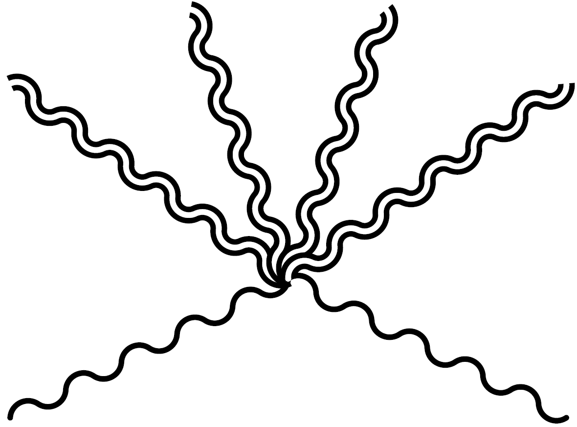
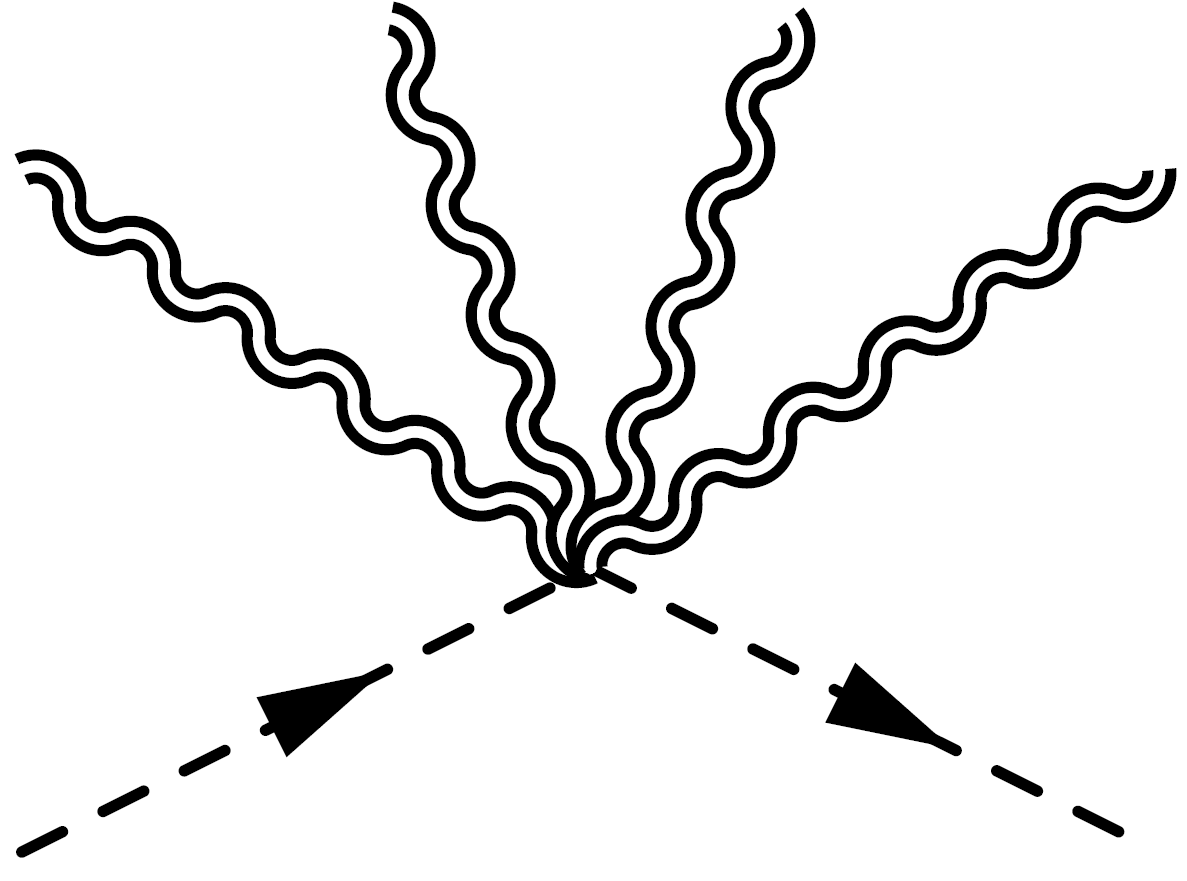
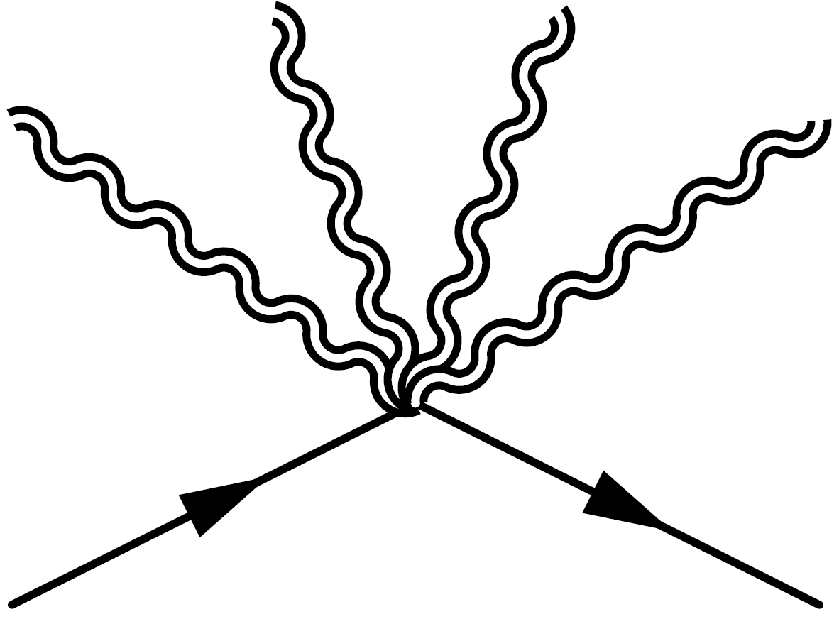
Figure 1: Feynman diagrams of the emission vertex of 4 gauge bosons from the gauge clouds (double wiggly lines) by a gauge boson (left, single wiggly line), a scalar (middle, dashed line) and a fermion (right, plain line).

The pure gauge sector of the FSM is described by the Lagrangian

$$\mathcal{L}_{\text{gauge}} =-\dfrac{1}{2}\,\text{tr}\left[\mathcal{G}_{\mu\nu}\star_{c}\mathcal{G}^{\mu\nu}\right]-\dfrac{1}{2}\,\text{tr}\left[\mathcal{W}_{\mu\nu}\star_{w}\mathcal{W}^{\mu\nu}\right]-\dfrac{1}{4}\,\mathcal{B}_{\mu\nu}\star_{0}\mathcal{B}^{\mu\nu}$$ (13)

$$\supseteq-\dfrac{1}{4}\,\mathcal{G}_{\ \mu\nu}^{a}\ast_{c}\mathcal{G}^{\ \mu\nu}_{a}-\dfrac{1}{4}\,\mathcal{W}_{\ \mu\nu}^{a}\ast_{w}\mathcal{W}^{\ \mu\nu}_{a}-\dfrac{1}{4}\,\mathcal{B}_{\mu\nu}\ast_{0}\mathcal{B}^{\mu\nu}\,,$$ (14)

where the terms that are not displayed in the second line correspond to the gauge cloud that does not contribute to the tree-level propagators. Since $SU(3)_{C}$ is not affected by EWSB, one can already extract the gluon propagator in the Feynman-’t Hooft gauge:

$$\Pi_{G}^{ab\mu\nu}(p^{2})=\dfrac{-ie^{-\vartheta_{c}\left(\eta_{c}\,p^{2}\right)}}{p^{2}+i\epsilon}\,\delta^{ab}g^{\mu\nu}\,,$$ (15)

which has only the canonical pole at $p^{2}=0$, aka the gluon, like in local quantum chromodynamics.

2.2 Electroweak Symmetry Breaking

In the GWS model, EWSB occurs by tachyon condensation of the Higgs field, where $SU(2)_{W}\times U(1)_{Y}\rightarrow U(1)_{em}$. In the physical EW vacuum, the gauge symmetry $SU(2)_{W}\times U(1)_{Y}$ is nonlinearly realized. As for the gauge fields, one introduces the covariant $\star_{h}$ and noncovariant $\ast_{h}$ star-products between the fields in the representations of the Higgs tachyon that are the complex conjugates of each other:

$$H(x)^{\dagger}\ast_{h}H(x) \equiv H^{\dagger}(x)\,e^{\vartheta\left(\overleftarrow{\partial_{\mu}}\,\eta^{\mu\nu}_{h}\,\overrightarrow{\partial_{\nu}}\right)}\,H(x)\,,$$ (16)

$$H^{\dagger}(x)\star_{h}H(x) \equiv H^{\dagger}(x)\,e^{\vartheta\left(\overleftarrow{\mathcal{D}_{\mu}}\,\eta^{\mu\nu}_{h}\,\overrightarrow{\mathcal{D}_{\nu}}\right)}\,H(x)$$ (17)

$$=\left.e^{\vartheta\left(\mathcal{D}_{\mu}^{y}\,\eta^{\mu\nu}_{h}\,\mathcal{D}_{\nu}^{z}\right)}\,H^{\dagger}(y)\cdot H(z)\right|_{y=z=x}$$ (18)

$$=H^{\dagger}(x)\ast_{h}H(x)+\mathcal{O}\left(\dfrac{g_{1}}{\Lambda_{h}^{4}}\,B|H|^{2}\right)+\mathcal{O}\left(\dfrac{g_{2}}{\Lambda_{h}^{4}}\,W|H|^{2}\right)\,,$$ (19)

with the tensor $\eta_{h}^{\mu\nu}=\eta_{h}\,g^{\mu\nu}$, the covariant derivative $\mathcal{D}_{\mu}H^{\dagger}=\left(\mathcal{D}_{\mu}H\right)^{\dagger}$, the commutator $\left[\mathcal{D}_{\mu}^{y},\mathcal{D}_{\nu}^{z}\right]=0$ if $y\neq z$, and the gauge clouds (cf. Fig. 1) in the ellipses $\mathcal{O}(\cdots)$. Note that the star-products are Hermitian symmetric. One can then build the following Lagrangian for the kinetic and potential terms of the Higgs tachyon:

$$\mathcal{L}_{\text{Higgs}} =\mathcal{D}_{\mu}H^{\dagger}\star_{h}\mathcal{D}^{\mu}H+\mu^{2}\,H^{\dagger}\star_{h}H-\lambda\,\left(H^{\dagger}\star_{h}H\right)\star_{0}\left(H^{\dagger}\star_{h}H\right)\,.$$ (20)

With the quartic Higgs self-coupling, one has an example where the nonassociativity of the star-products enters the game: one needs to explicitly write the parentheses. Then, one performs the replacement $\left(\star_{h}\mapsto\ast_{h}\right)$ in Eq. (20), i.e. one drops the gauge cloud from the covariant star-products of Higgs tachyons. Indeed, one can see that this gauge cloud does not contribute to the tree-level propagators after EWSB by using the properties

$$v\ast_{h}H(x)=v\cdot H(x)\ \ \ \text{and}\ \ \ v\star_{h}v=v^{2}+\mathcal{O}(W^{4})+\mathcal{O}(B^{4})\,,$$ (21)

where $v$ is the vev of the Higgs field. As discussed in Ref. Nortier:2023dkq and Fig. 2, without the condition $\vartheta_{h}(-z)=\vartheta_{h}(z)$, the gauge cloud that dresses the product of Higgs vev’s starts in general at $\mathcal{O}(W^{2})$ and $\mathcal{O}(B^{2})$. One can check that such quadratic pointwise products of gauge bosons would contribute to the mass of the weak bosons in the physical EW vacuum: it would spoil the ghost-free property of the model.

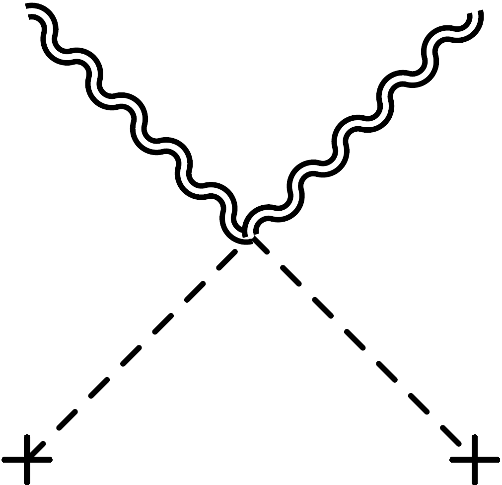
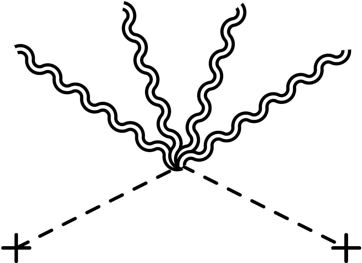
Figure 2: Feynman diagrams in unitary gauge, where blobs are a nonlocal vertices, crosses are insertions of Higgs vev’s, single wiggly lines are gauge bosons from the Lagrangian with the replacement $\star\mapsto\ast$, whereas double wiggly lines are gauge bosons coming from the local expansion of the gauge clouds. Left: the covariant derivatives in the quadratic term in Higgs tachyons of Eq. (23) implies an interaction between a gauge boson with 2 insertions of Higgs vev’s, giving a nonlocal contribution to the mass term of the gauge boson. Middle: when $\vartheta_{h}(-z)\neq\vartheta_{h}(z)$, the gauge cloud in the Higgs potential of Eq. (20) implies in general a local interaction between a gauge boson with 2 insertions of Higgs vev’s, giving a local contribution to the mass term of the gauge boson. Right: when $\vartheta_{h}(-z)=\vartheta_{h}(z)$, the insertion of Higgs vev’s from the gauge cloud in the Higgs potential starts to interact with the gauge bosons with a quartic self-interaction but does not contribute to the mass term of the gauge boson.

Consider the polar representation of the Higgs tachyon around its vev as

$$H=e^{\frac{i\pi^{a}(x)\sigma_{a}}{v}}\,H_{U}\,,\ \ \ H_{U}(x)=\dfrac{1}{\sqrt{2}}\begin{pmatrix}0\\ v+h(x)\end{pmatrix}\,,\ \ \ v=\sqrt{\dfrac{\mu^{2}}{\lambda}}\,,$$ (22)

where $h(x)$ is the radial mode, aka the Higgs boson. In order to study the physical spectrum, one chooses the unitary gauge, where the pion fields $\pi^{a}(x)$ are eaten by the $W_{\mu}$ and $B_{\mu}$ gauge bosons, such that $H(x)\equiv H_{U}(x)$. One can then extract the vector boson masses from the quadratic term in Higgs tachyons with covariant derivatives:

$$\mathcal{D}_{\mu}H_{U}^{\dagger}\ast_{h}\mathcal{D}^{\mu}H_{U} =\dfrac{1}{2}\left[\begin{pmatrix}0&v\end{pmatrix}\cdot\left(\dfrac{g_{2}}{2}\,W_{\mu}^{a}\sigma_{a}+\dfrac{g_{1}}{2}B_{\mu}\right)\right]\ast_{h}\left[\left(\dfrac{g_{2}}{2}\,W_{\mu}^{b}\sigma_{b}+\dfrac{g_{1}}{2}B^{\mu}\right)\cdot\begin{pmatrix}0\\ v\end{pmatrix}\right]$$

$$=\dfrac{v^{2}}{8}\left[g_{2}^{2}\left(W_{\mu}^{1}\ast_{h}W^{\mu}_{1}+W_{\mu}^{2}\ast_{h}W^{\mu}_{2}\right)\right.$$

$$+\left.\left(-g_{2}\,W_{\mu}^{3}+g_{1}\,B_{\mu}\right)\ast_{h}\left(-g_{2}\,W^{\mu}_{3}+g_{1}\,B^{\mu}\right)\right]\,.$$ (23)

These mass terms mix the $W_{\mu}^{3}$ and $B_{\mu}$ fields, and one must ensure that they combine with the kinetic terms in Eq. (14) to give ghost-free propagators for the massive vector bosons of the form

$$\dfrac{-ie^{-\vartheta_{\bullet}\left(\eta_{\bullet}\,p^{2}\right)}}{p^{2}-m_{\bullet}^{2}+i\epsilon}\left(g^{\mu\nu}-\dfrac{p^{\mu}p^{\nu}}{m_{\bullet}^{2}}\right)\,.$$ (24)

For this to happen, the involved noncovariant star-products must be the same:

$$\ast_{w}\equiv\ast_{0}\equiv\ast_{h}\ \ \Rightarrow\ \ \eta_{w}=\eta_{0}=\eta_{h}\,,\ \ \vartheta_{w}(z)=\vartheta_{0}(z)=\vartheta_{h}(z)\,.$$ (25)

Otherwise, the WNL form factors do not factorize between the kinetic and mass terms, and the ghost-free condition is spoiled Nortier:2023dkq .

Now, one can introduce the physical vector bosons:

$$W_{\mu}^{\pm}=\dfrac{1}{\sqrt{2}}\left(W_{\mu}^{1}\mp W_{\mu}^{2}\right)\,,\ \ \ \begin{pmatrix}Z_{\mu}\\ A_{\mu}\end{pmatrix}=\begin{pmatrix}\cos\theta_{w}&-\sin\theta_{w}\\ \sin\theta_{w}&\cos\theta_{w}\end{pmatrix}\begin{pmatrix}W^{3}_{\mu}\\ B_{\mu}\end{pmatrix}\,.$$ (26)

The weak mixing angle $\theta_{w}$ and the $U(1)_{em}$ gauge coupling $g_{e}$ are defined as usual:

$$\tan\theta_{w}=\dfrac{g_{1}}{g_{2}}\,,\ \ \ g_{e}=g_{2}\,\sin\theta_{w}\,.$$ (27)

The quadratic Lagrangian of the physical vector bosons reads

$$-\dfrac{1}{4}\,\mathcal{A}_{\mu\nu}\ast_{w}\mathcal{A}^{\mu\nu}-\dfrac{1}{2}\,\mathcal{W}_{\mu\nu}^{+}\ast_{w}\mathcal{W}^{-\mu\nu}-\dfrac{1}{4}\,\mathcal{Z}_{\mu\nu}\ast_{w}\mathcal{Z}^{\mu\nu}$$

$$+\dfrac{M_{A}^{2}}{2}\,A_{\mu}\ast_{w}A^{\mu}+M_{W}^{2}\,W^{+}_{\mu}\ast_{w}W^{-\mu}+\dfrac{M_{Z}^{2}}{2}\,Z_{\mu}\ast_{w}Z^{\mu}\,,$$ (28)

$$\text{with}\ M_{W}=g_{2}\,\dfrac{v}{2}\,,\ M_{Z}=\dfrac{M_{W}}{\cos\theta_{w}}\ \ \text{and}\ \ M_{A}=0\,,$$ (29)

and the field strength tensors

$$\mathcal{W}_{\mu\nu}^{\pm}=\partial_{\mu}W^{\pm}_{\nu}-\partial_{\nu}W^{\pm}_{\mu}\,,\ \ \ \mathcal{Z}_{\mu\nu}=\partial_{\mu}Z_{\nu}-\partial_{\nu}Z_{\mu}\,,\ \ \ \mathcal{A}_{\mu\nu}=\partial_{\mu}A_{\nu}-\partial_{\nu}A_{\mu}\,.$$ (30)

From this quadratic Lagrangian, one gets the propagators for the photon $A_{\mu}$ and the weak bosons $V_{\mu}=Z_{\mu}$ or $W_{\mu}^{\pm}$ in Feynman and unitary gauges, respectively:

$$\Pi_{A}^{\mu\nu}(p^{2})=\dfrac{-ie^{-\vartheta_{w}\left(\eta_{w}\,p^{2}\right)}}{p^{2}+i\epsilon}\,g^{\mu\nu}\,,\ \ \ \Pi_{V}^{\mu\nu}(p^{2})=\dfrac{-ie^{-\vartheta_{w}\left(\eta_{w}\,p^{2}\right)}}{p^{2}-M_{V}^{2}+i\epsilon}\left(g^{\mu\nu}-\dfrac{p^{\mu}p^{\nu}}{m_{V}^{2}}\right)\,.$$ (31)

Concerning the Higgs boson $h(x)$, its quadratic Lagrangian is

$$\mathcal{L}_{\text{Higgs}}\supseteq\dfrac{1}{2}\,\partial_{\mu}h\ast_{w}\partial^{\mu}h-\dfrac{M_{H}^{2}}{2}\,h\ast_{w}h\,,$$ (32)

$$\text{with}\ M_{H}=\sqrt{2}\mu=\sqrt{2\lambda}v\,,$$ (33)

and one gets the ghost-free propagator

$$\Pi_{h}(p^{2})=\dfrac{ie^{-\vartheta_{w}\left(\eta_{w}\,p^{2}\right)}}{p^{2}-M_{H}^{2}+i\epsilon}\,.$$ (34)

This analysis shows that there is no ghost at tree-level in the bosonic sector of the proposed FSM. As discussed in detail in Ref. Nortier:2023dkq , the main difference with the usual string-inspired models of the literature Gama:2018cda ; Hashi:2018kag ; Koshelev:2020fok ; Nortier:2023dkq is that both the kinetic term and the potential of the Higgs field are smeared via the star-products. Instead, in string-inspired models, only the fields in either the quadratic or the self-interaction terms are smeared, but not in both. In addition, the other crucial properties for a ghost-free FSM are the linearity and the Hermitian symmetry of the star-products, combined with the properties of the gauge cloud in Eq. (21).

A very important observation for the phenomenology of the FSM is that the tree-level expressions of the particle masses after EWSB are the same as in the SM in terms of the Lagrangian parameters. This means that the difference between the perturbative spectra of the 2 models arises only at loop-level. This is in contrast with what happens when EWSB occurs in the string-inspired formalism that is not ghost-free Gama:2018cda ; Hashi:2018kag ; Krasnikov:2022xsi .

3 Fermionic Fields

3.1 Dirac & Weyl Fermions

Since the fundamental building blocks of the SM fermions are Weyl spinors, where different chiralities belong to different representations of the EW gauge group, one considers the Dirac $\gamma$-matrices in the chiral representation, and the chirality projectors are given by

$$P_{R}=\dfrac{1+\gamma^{5}}{2}\,,\ \ \ P_{L}=\dfrac{1-\gamma^{5}}{2}\,,\ \ \ \text{with}\ \ \ \gamma^{5}=i\gamma^{0}\gamma^{1}\gamma^{2}\gamma^{3}\,.$$ (35)

We work in the 4-component formalism where, for a spinor $\psi$, the chiral decomposition $\psi=\psi_{L}+\psi_{R}$ is given by $\psi_{L}=P_{L}\,\psi$ and $\psi_{R}=P_{R}\,\psi$.

It is tempting to define different star-products for different chiralities, where the kinetic terms would be

$$\overline{\psi}_{L}\star_{L}\left(\dfrac{i}{2}\,\gamma^{\mu}\partial_{\mu}\psi_{L}\right)+\overline{\psi}_{R}\star_{R}\left(\dfrac{i}{2}\,\gamma^{\mu}\partial_{\mu}\psi_{R}\right)+\text{H.c.}\,.$$ (36)

Nevertheless, mass terms mix chiralities, which imposes the same expression for the noncovariant star-product:

$$-M_{\psi}\left(\overline{\psi}_{L}\ast_{?}\psi_{R}+\overline{\psi}_{R}\ast_{?}\psi_{L}\right)\ \ \ \Rightarrow\ \ \ \ast_{?}\equiv\ast_{L}\equiv\ast_{R}\,,$$ (37)

in order to get a ghost-free propagator for a Dirac fermion of the form

$$\dfrac{ie^{-\vartheta_{\psi}\left(\eta_{\psi}\,p^{2}\right)}}{\gamma\cdot p-M_{\psi}+i\epsilon}\,.$$ (38)

As for the bosons, one defines the covariant $\star_{\psi}$ and noncovariant $\ast_{\psi}$ star-products between 2 elementary/composite fermions in the complex conjugate gauge representation of each other:

$$\overline{\Psi}(x)\ast_{\psi}\Psi(x) =\overline{\Psi}(x)\,e^{\vartheta\left(\overleftarrow{\partial_{\mu}}\,\eta_{\psi}^{\mu\nu}\,\overrightarrow{\partial_{\nu}}\right)}\,\Psi(x)\,,$$ (39)

$$\overline{\Psi}(x)\star_{\psi}\Psi(x) =\overline{\Psi}(x)\,e^{\vartheta\left(\overleftarrow{\mathcal{D}_{\mu}}\,\eta_{\psi}^{\mu\nu}\,\overrightarrow{\mathcal{D}_{\nu}}\right)}\,\Psi(x)$$ (40)

$$=\overline{\Psi}(x)\ast_{\psi}\Psi(x)+\text{gauge cloud}\,,$$ (41)

with $\overline{\Psi}=\Psi^{\dagger}\gamma^{0}$, the covariant derivative $\mathcal{D}_{\mu}\Psi^{\dagger}=\left(\mathcal{D}_{\mu}\Psi\right)^{\dagger}$, and the tensor

$$\eta_{\psi}^{\mu\nu}=\eta_{\psi}^{+}\,g^{\mu\nu}+i\eta_{\psi}^{-}\,\gamma^{\mu\nu}\,,$$ (42)

that is defined with the symmetric and antisymmetric rank 2 tensors made with the $\gamma$-matrices:

$$g^{\mu\nu}=\dfrac{1}{2}\left\{\gamma^{\mu},\gamma^{\nu}\right\}\,,\ \ \ \gamma^{\mu\nu}=\dfrac{1}{2}\left[\gamma^{\mu},\gamma^{\nu}\right]\,,$$ (43)

respectively. Note that one can (a priori) associate 2 different fuzzy-plaquettes $\eta_{\psi}^{\pm}=\left(1/\Lambda_{\psi}^{\pm}\right)^{2}$ to 1 fermion field. Again, fermions are dressed by gauge clouds (cf. Fig. 1). The gauge-invariant kinetic terms for the fermions are given by

$$\mathcal{L}_{\text{kinetic}} =\overline{Q}_{L}^{i}\star_{q}\left(\dfrac{i}{2}\,\delta_{ij}\gamma^{\mu}\mathcal{D}_{\mu}Q_{L}^{j}\right)+\overline{d}_{R}^{i}\star_{q}\left(\dfrac{i}{2}\,\delta_{ij}\gamma^{\mu}\mathcal{D}_{\mu}d_{R}^{j}\right)+\overline{u}_{R}^{i}\star_{q}\left(\dfrac{i}{2}\,\delta_{ij}\gamma^{\mu}\mathcal{D}_{\mu}u_{R}^{j}\right)$$

$$+\overline{L}_{L}^{i}\star_{\ell}\left(\dfrac{i}{2}\,\delta_{ij}\gamma^{\mu}\mathcal{D}_{\mu}L_{L}^{j}\right)+\overline{e}_{R}^{i}\star_{\ell}\left(\dfrac{i}{2}\,\delta_{ij}\gamma^{\mu}\mathcal{D}_{\mu}e_{R}^{j}\right)+\text{H.c.}\,,$$ (44)

where one has a star-product $\star_{q}$ for quarks and another one $\star_{\ell}$ for leptons. We comment on the choice of the same star-product for different generations in the following section.

3.2 Yukawa Sector

In order to write gauge-invariant Yukawa terms, with the covariant star-products between chiral fermions in different representations of the EW gauge group, one can use the composite fields made of 1 chiral fermion and 1 Higgs tachyon (built with the usual pointwise product). For 1 generation, one can propose the following Lagrangian with positive Yukawa couplings:

$$\mathcal{L}_{\text{Yukawa}}^{(1)} =-\lambda_{d}\left(\overline{Q}_{L}\cdot H\right)\star_{q}d_{R}-\lambda_{u}\left(\overline{Q}_{L}\cdot\overline{H}\right)\star_{q}u_{R}-\lambda_{e}\left(\overline{L}_{L}\cdot H\right)\star_{\ell}e_{R}+\text{H.c.}$$ (45)

$$\supseteq-m_{d}\,\overline{d}_{L}\ast_{q}d_{R}-m_{u}\,\overline{u}_{L}\ast_{q}u_{R}-m_{e}\,\overline{e}_{L}\ast_{\ell}e_{R}+\text{H.c.}\,,$$ (46)

$$\text{with}\ \ \ m_{d}=\dfrac{\lambda_{d}v}{\sqrt{2}}\,,\ \ \ m_{u}=\dfrac{\lambda_{u}v}{\sqrt{2}}\,,\ \ \ m_{e}=\dfrac{\lambda_{e}v}{\sqrt{2}}\,,\ \ \$$ (47)

where the mass terms of the second line are extracted from the quadratic terms involving the noncovariant star-products (like for the boson fields). Again, the tree-level spectrum is ghost-free and is the same as in the SM with 1 generation.

The generalization to several generations with complex Yukawa couplings is straightforward: one considers the Lagrangian

$$\mathcal{L}_{\text{Yukawa}}=-\lambda_{d}^{ij}\left(\overline{Q}_{L}^{i}\cdot H\right)\star_{q}d_{R}^{j}-\lambda_{u}^{ij}\left(\overline{Q}_{L}^{i}\cdot\overline{H}\right)\star_{q}u_{R}^{j}-\lambda_{e}^{ij}\left(\overline{L}_{L}^{i}\cdot H\right)\star_{\ell}e_{R}^{j}+\text{H.c.}\,.$$ (48)

We stress that it is necessary to use the same covariant star-products between different generations that belong to the same gauge representation. Indeed, the WNL form factors in the mass and kinetic terms need to factorize to keep ghost-free propagators, as in Eq. (38). It follows that both the covariant and noncovariant star-products are linear in flavor space, so the flavor rotations:

$$\text{Quarks:}\ \ \ d_{L}^{i}\mapsto U_{d}^{ij}d_{L}^{j}\,,\ \ \ d_{R}^{i}\mapsto W_{d}^{ij}d_{R}^{j}\,,\ \ \ u_{L}^{i}\mapsto U_{u}^{ij}u_{L}^{j}\,,\ \ \ u_{R}^{i}\mapsto W_{u}^{ij}u_{R}^{j}\,,$$ (49)

$$\text{Leptons:}\ \ \ e_{L}^{i}\mapsto U_{e}^{ij}e_{L}^{j}\,,\ \ \ e_{R}^{i}\mapsto W_{e}^{ij}e_{R}^{j}\,,\ \ \ \nu_{L}^{i}\mapsto U_{\nu}^{ij}\nu_{L}^{j}\,,$$ (50)

can go through the star-products without complications. By using the usual field redefinition procedure Peskin:1995ev , it is thus straightforward to show that the FSM has the same qualitative features as the SM concerning flavor mixing, which are encoded in the CKM matrix: there is only 1 physical $CP$-violating phase coming from the Yukawa couplings (with 3 fermion generations) and no FCNC’s at tree-level via the GIM mechanism.

4 Conclusion & Outlook

In this letter, we have proposed the FSM: a WNL extension of the SM based on the covariant star-product formalism introduced in Ref. Nortier:2023dkq . We have generalized the previous article by including non-Abelian gauge symmetries and fermions. Our main achievement is to realize EWSB without introducing ghosts in the physical EW vacuum, which is the main drawback of the previous string-inspired attempts Gama:2018cda ; Hashi:2018kag ; Koshelev:2020fok ; Nortier:2023dkq . As mentioned in the introduction, 2 alternative proposals have already been published that differ from our approach in their construction:

• Gauge-Higgs Unification Hashi:2018kag : The Higgs sector arises from the dimensional reduction of a 6D gauge theory. Our proposal is more minimal, since we do not need to add extra compact dimensions, and there are no extra elementary particles other than those already present in the SM.

• Tree-Duality Modesto:2021okr : This formalism shares several features with our proposal: there are no new fields beyond the SM, and it is realized as a WNL deformation of a local “mother theory”. However, it is built from the constraint to have the same tree-level scattering amplitudes as the mother theory Modesto:2021ief ; Modesto:2021soh ; Calcagni:2023goc .

Our construction looks promising, but several issues remain to be investigated, both from the theoretical and phenomenological points of view. From the theoretical side, the following points would be interesting to address:

• The inclusion of gravity (the modern motivation for WNL) with the covariant star-product formalism deserves to be discussed elsewhere.

• Our analysis remains at tree-level, and it is thus crucial to study the UV-behavior of the quantum corrections in the FSM, as well as the issue of ghosts at loop-level Shapiro:2015uxa . For these purposes, one needs to specify the exponent functions $\vartheta_{\bullet}(z)$.

From the phenomenological side, several directions are possible:

• It has been argued in some toy models that string-inspired WNL provides a mechanism to stabilize the weak scale (and more generally the Higgs potential) under radiative corrections Krasnikov:1987yj ; Biswas:2014yia ; Ghoshal:2017egr ; Abu-Ajamieh:2023syy , implying interests for looking at WNL signatures at current particle physics experiments Biswas:2014yia ; Su:2021qvm ; Capolupo:2022awe ; Capolupo:2023kuu ; Abu-Ajamieh:2023txh . If also true in the FSM, it might provide a concrete framework to discuss the implications on the infamous gauge hierarchy problem.

• The FSM offers a new scenario where deviations from the SM are not associated with new particles, and it is worth understanding its underlying phenomenology. Moreover, once Taylor expanded, the WNL form factors imply corrections of $\mathcal{O}\left(1/\Lambda_{\bullet}^{4}\right)$ to the SM at tree-level, i.e. dimension 8 operators, whereas one typically expects $\mathcal{O}(1)$ contributions to the Wilson coefficients of dimension 6 operators by integrating out new heavy fields at tree-level Falkowski:2023hsg .

• The FSM does not introduce new operators violating the baryon and lepton numbers at the perturbative level. Furthermore, in the limit of vanishing Yukawa couplings, the FSM exhibits the same flavor symmetry group as the SM:

  $$U(3)_{Q}\times U(3)_{u}\times U(3)_{d}\times U(3)_{L}\times U(3)_{e}\,.$$ (51)

  Since the star-products introduce a WNL deformation of the local Yukawa operators, the breaking effects are also controlled by the standard Yukawa couplings, with subleading contributions coming from higher-dimensional operators suppressed by the nonlocal scales. Therefore, the FSM offers a framework where the contributions to the breaking of flavor symmetries are naturally suppressed, for the same reason they are suppressed in the SM.

• Some speculations in WNL theories about the existence of bound states made of SM particles that are confined via the higher-derivative form factors can be found in Refs. Tomboulis:1997gg ; Modesto:2015lna ; Mo:2022szw . If true in the FSM, it would be interesting to study their phenomenology and experimental signatures.

- (1) F. Halzen and A.D. Martin, Quarks & Leptons: An Introductory Course in Modern Particle Physics, Wiley (1984).
- (2) A. Marshakov, String theory or field theory?, Phys. Usp. 45 (2002) 915 [hep-th/0212114].
- (3) S.B. Giddings, The gravitational S-matrix: Erice lectures, Subnucl. Ser. 48 (2013) 93 [1105.2036].
- (4) L. Buoninfante, G. Lambiase and A. Mazumdar, Ghost-free infinite derivative quantum field theory, Nucl. Phys. B 944 (2019) 114646 [1805.03559].
- (5) L. Modesto, Super-renormalizable quantum gravity, Phys. Rev. D 86 (2012) 044005 [1107.2403].
- (6) T. Biswas, E. Gerwick, T. Koivisto and A. Mazumdar, Towards Singularity- and Ghost-Free Theories of Gravity, Phys. Rev. Lett. 108 (2012) 031101 [1110.5249].
- (7) T. Biswas, A. Conroy, A.S. Koshelev and A. Mazumdar, Generalized ghost-free quadratic curvature gravity, Class. Quant. Grav. 31 (2014) 015022 [1308.2319].
- (8) G. Calcagni and L. Modesto, Nonlocal quantum gravity and M-theory, Phys. Rev. D 91 (2015) 124059 [1404.2137].
- (9) S. Talaganis, T. Biswas and A. Mazumdar, Towards understanding the ultraviolet behavior of quantum loops in infinite-derivative theories of gravity, Class. Quant. Grav. 32 (2015) 215017 [1412.3467].
- (10) S. Talaganis and A. Mazumdar, High-energy scatterings in infinite-derivative field theory and ghost-free gravity, Class. Quant. Grav. 33 (2016) 145005 [1603.03440].
- (11) S. Abel, L. Buoninfante and A. Mazumdar, Nonlocal gravity with worldline inversion symmetry, JHEP 01 (2020) 003 [1911.06697].
- (12) T. Biswas and N. Okada, Towards LHC physics with nonlocal Standard Model, Nucl. Phys. B 898 (2015) 113 [1407.3331].
- (13) A. Ghoshal, A. Mazumdar, N. Okada and D. Villalba, Stability of infinite derivative Abelian Higgs models, Phys. Rev. D 97 (2018) 076011 [1709.09222].
- (14) L. Buoninfante, A. Ghoshal, G. Lambiase and A. Mazumdar, Transmutation of nonlocal scale in infinite derivative field theories, Phys. Rev. D 99 (2019) 044032 [1812.01441].
- (15) A. Ghoshal, A. Mazumdar, N. Okada and D. Villalba, Nonlocal non-Abelian gauge theory: Conformal invariance and -function, Phys. Rev. D 104 (2021) 015003 [2010.15919].
- (16) M. Frasca and A. Ghoshal, Mass gap in strongly coupled infinite derivative non-local Higgs: Dyson–Schwinger approach, Class. Quant. Grav. 38 (2021) 175013 [2011.10586].
- (17) M. Frasca and A. Ghoshal, Diluted mass gap in strongly coupled non-local Yang-Mills, JHEP 21 (2020) 226 [2102.10665].
- (18) M. Frasca, A. Ghoshal and N. Okada, Confinement and renormalization group equations in string-inspired nonlocal gauge theories, Phys. Rev. D 104 (2021) 096010 [2106.07629].
- (19) M. Frasca, A. Ghoshal and A.S. Koshelev, Quintessence dark energy from strongly-coupled higgs mass gap: local and non-local higher-derivative non-perturbative scenarios, Eur. Phys. J. C 82 (2022) 1108 [2203.15020].
- (20) A. Chatterjee, M. Frasca, A. Ghoshal and S. Groote, Re-normalisable Non-local Quark-Gluon Interaction: Mass Gap, Chiral Symmetry Breaking & Scale Invariance, 2302.10944.
- (21) F. Abu-Ajamieh and S.K. Vempati, A Proposed Renormalization Scheme for Non-local QFTs and Application to the Hierarchy Problem, 2304.07965.
- (22) G.V. Efimov, Analytic properties of Euclidean amplitudes, Sov.J.Nucl.Phys. 4 (1967) 309.
- (23) R. Pius and A. Sen, Cutkosky rules for superstring field theory, JHEP 10 (2016) 024 [1604.01783].
- (24) C.D. Carone, Unitarity and microscopic acausality in a nonlocal theory, Phys. Rev. D 95 (2017) 045009 [1605.02030].
- (25) R. Pius and A. Sen, Unitarity of the box diagram, JHEP 11 (2018) 094 [1805.00984].
- (26) F. Briscese and L. Modesto, Cutkosky rules and perturbative unitarity in Euclidean nonlocal quantum field theories, Phys. Rev. D 99 (2019) 104043 [1803.08827].
- (27) P. Chin and E.T. Tomboulis, Nonlocal vertices and analyticity: Landau equations and general Cutkosky rule, JHEP 06 (2018) 014 [1803.08899].
- (28) C. De Lacroix, H. Erbin and A. Sen, Analyticity and crossing symmetry of superstring loop amplitudes, JHEP 05 (2019) 139 [1810.07197].
- (29) F. Briscese and L. Modesto, Non-unitarity of Minkowskian non-local quantum field theories, Eur. Phys. J. C 81 (2021) 730 [2103.00353].
- (30) A.S. Koshelev and A. Tokareva, Unitarity of Minkowski nonlocal theories made explicit, Phys. Rev. D 104 (2021) 025016 [2103.01945].
- (31) L. Buoninfante, Contour prescriptions in string-inspired nonlocal field theories, Phys. Rev. D 106 (2022) 126028 [2205.15348].
- (32) N.V. Krasnikov, Nonlocal gauge theories, Theor. Math. Phys. 73 (1987) 1184.
- (33) A. Ghoshal and F. Nortier, Fate of the false vacuum in string-inspired nonlocal field theory, JCAP 08 (2022) 047 [2203.04438].
- (34) A. Ghoshal, Scalar dark matter probes the scale of nonlocality, Int. J. Mod. Phys. A 34 (2019) 1950130 [1812.02314].
- (35) N.V. Krasnikov, Nonlocal GUT, Mod. Phys. Lett. A 36 (2021) 2150104 [2012.10161].
- (36) F. Abu-Ajamieh, P. Chattopadhyay, A. Ghoshal and N. Okada, Anomalies in String-inspired Non-local Extensions of QED, 2307.01589.
- (37) F. Nortier, Extra Dimensions and Fuzzy Branes in String-inspired Nonlocal Field Theory, Acta Phys. Polon. B 54 (2023) 6 A2 [2112.15592].
- (38) A.S. Koshelev, K.S. Kumar and A.A. Starobinsky, Cosmology in nonlocal gravity, 2305.18716.
- (39) L. Buoninfante, B.L. Giacchini and T. de Paula Netto, Black holes in non-local gravity, 2211.03497.
- (40) J. Terning, Gauging nonlocal Lagrangians, Phys. Rev. D 44 (1991) 887.
- (41) I.L. Shapiro, Counting ghosts in the “ghost-free” non-local gravity, Phys. Lett. B 744 (2015) 67 [1502.00106].
- (42) J.C. Collins, Renormalization: An Introduction to Renormalization, The Renormalization Group, and the Operator Product Expansion, Cambridge Monographs on Mathematical Physics, Cambridge University Press (1986), 10.1017/CBO9780511622656.
- (43) Y.V. Kuz’min, The Convergent Nonlocal Gravitation, Sov. J. Nucl. Phys. 50 (1989) 1011.
- (44) E.T. Tomboulis, Superrenormalizable gauge and gravitational theories, hep-th/9702146.
- (45) A. Bas i Beneito, G. Calcagni and L. Rachwał, Classical and quantum nonlocal gravity, 2211.05606.
- (46) L. Modesto and L. Rachwal, Super-renormalizable and finite gravitational theories, Nucl. Phys. B 889 (2014) 228 [1407.8036].
- (47) L. Modesto and L. Rachwał, Universally finite gravitational and gauge theories, Nucl. Phys. B 900 (2015) 147 [1503.00261].
- (48) L. Modesto, M. Piva and L. Rachwal, Finite quantum gauge theories, Phys. Rev. D 94 (2016) 025021 [1506.06227].
- (49) E.T. Tomboulis, Renormalization and unitarity in higher derivative and nonlocal gravity theories, Mod. Phys. Lett. A 30 (2015) 1540005.
- (50) L. Modesto and L. Rachwal, Finite Conformal Quantum Gravity and Nonsingular Spacetimes, 1605.04173.
- (51) L. Modesto, L. Rachwał and I.L. Shapiro, Renormalization group in super-renormalizable quantum gravity, Eur. Phys. J. C 78 (2018) 555 [1704.03988].
- (52) L. Modesto and L. Rachwał, Nonlocal quantum gravity: A review, Int. J. Mod. Phys. D 26 (2017) 1730020.
- (53) A.S. Koshelev, K. Sravan Kumar, L. Modesto and L. Rachwał, Finite quantum gravity in dS and AdS spacetimes, Phys. Rev. D 98 (2018) 046007 [1710.07759].
- (54) N. Barnaby and N. Kamran, Dynamics with infinitely many derivatives: the initial value problem, JHEP 02 (2008) 008 [0709.3968].
- (55) F. Galli and A.S. Koshelev, Perturbative stability of SFT-based cosmological models, JCAP 05 (2011) 012 [1011.5672].
- (56) F.S. Gama, J.R. Nascimento, A.Y. Petrov and P.J. Porfirio, Spontaneous Symmetry Breaking in the Nonlocal Scalar QED, 1804.04456.
- (57) M.N. Hashi, H. Isono, T. Noumi, G. Shiu and P. Soler, Higgs mechanism in nonlocal field theories, JHEP 08 (2018) 064 [1805.02676].
- (58) A.S. Koshelev and A. Tokareva, Nonlocal self-healing of Higgs inflation, Phys. Rev. D 102 (2020) 123518 [2006.06641].
- (59) F. Nortier, Exorcizing Ghosts from the Vacuum Spectra in String-inspired Nonlocal Tachyon Condensation, Acta Phys. Polon. B 54 (2023) 9 A4 [2307.11741].
- (60) S.L. Glashow, Partial-symmetries of weak interactions, Nucl. Phys. 22 (1961) 579.
- (61) S. Weinberg, A Model of Leptons, Phys. Rev. Lett. 19 (1967) 1264.
- (62) A. Salam, Weak and Electromagnetic Interactions, Conf. Proc. C 680519 (1968) 367.
- (63) F. Englert and R. Brout, Broken Symmetry and the Mass of Gauge Vector Mesons, Phys. Rev. Lett. 13 (1964) 321.
- (64) P.W. Higgs, Broken Symmetries and the Masses of Gauge Bosons, Phys. Rev. Lett. 13 (1964) 508.
- (65) G.S. Guralnik, C.R. Hagen and T.W.B. Kibble, Global Conservation Laws and Massless Particles, Phys. Rev. Lett. 13 (1964) 585.
- (66) L. Modesto, The Higgs mechanism in nonlocal field theory, JHEP 06 (2021) 049 [2103.05536].
- (67) N. Cabibbo, Unitary Symmetry and Leptonic Decays, Phys. Rev. Lett. 10 (1963) 531.
- (68) M. Kobayashi and T. Maskawa, -Violation in the Renormalizable Theory of Weak Interaction, Prog. Theor. Phys. 49 (1973) 652.
- (69) S.L. Glashow, J. Iliopoulos and L. Maiani, Weak Interactions with Lepton-Hadron Symmetry, Phys. Rev. D 2 (1970) 1285.
- (70) M.E. Peskin and D.V. Schroeder, An Introduction to Quantum Field Theory, CRC Press (1995), 10.1201/9780429503559.
- (71) I. Hinchliffe, N. Kersting and Y.L. Ma, Review of the phenomenology of noncommutative geometry, Int. J. Mod. Phys. A 19 (2004) 179 [hep-ph/0205040].
- (72) N.V. Krasnikov, Nonlocal generalization of the SM as an explanation of recent CDF result, 2204.06327.
- (73) L. Modesto, Nonlocal Spacetime-Matter, 2103.04936.
- (74) L. Modesto and G. Calcagni, Tree-level scattering amplitudes in nonlocal field theories, JHEP 10 (2021) 169 [2107.04558].
- (75) G. Calcagni, B.L. Giacchini, L. Modesto, T. de Paula Netto and L. Rachwal, Renormalizability of nonlocal quantum gravity coupled to matter, JHEP 09 (2023) 034 [2306.09416].
- (76) X.-F. Su, Y.-Y. Li, R. Nicolaidou, M. Chen, H.-Y. Wu and S. Paganis, High Higgs excess as a signal of non-local QFT at the LHC, Eur. Phys. J. C 81 (2021) 796 [2108.10524].
- (77) A. Capolupo, G. Lambiase and A. Quaranta, Muon anomaly and non-locality, Phys. Lett. B 829 (2022) 137128 [2206.06037].
- (78) A. Capolupo, A. Quaranta and R. Serao, Phenomenological implications of nonlocal quantum electrodynamics, 2305.17992.
- (79) F. Abu-Ajamieh, N. Okada and S.K. Vempati, Corrected Calculation for the Non-local Solution to the g-2 Anomaly and Novel Results in Non-local QED, 2309.08417.
- (80) A. Falkowski, Lectures on SMEFT, Eur. Phys. J. C 83 (2023) 656.
- (81) Z. Mo, T. de Paula Netto, N. Burzilla and L. Modesto, Stringballs and Planckballs for dark matter, JHEP 07 (2022) 131 [2202.04540].