Brownian Fluctuations of a non-confining potential
Abstract
Brownian fluctuations arise for any quantity that depends on the stochastic variables of a Brownian particle. In this study, we explore the Brownian fluctuations of a bidimensional quadratic potential that exhibits two regimes: a confining regime and a non-confining regime. We divide the total potential into two contributions and analyze the mean, variance, skewness, excess kurtosis, and their distributions for each contribution as well as for the total potential. Our analysis offers an understanding into the statistical behavior of each quantity.
I Introduction
Out of equilibrium systems display novel phenomena due to the relevance of fluctuations. One of the simplest systems of this kind is the Brownian particle [1]. It is the minimal continuous system exhibiting diffusion and the influences of thermal fluctuations. The behavior of this kind of system is described not only by averages, but also by probability distributions [2].
In the field of Stochastic Thermodynamics [3, 4], distinct thermodynamic quantities such as heat, work, and entropy are linked to the behavior of Brownian particles [1]. These quantities fluctuate stochastically, as does the position of the particle itself. These Brownian fluctuations in these thermodynamic quantities have been extensively studied both theoretically [5, 6, 7, 8, 9, 10, 11, 12, 13, 14, 15, 16] and experimentally in a variety of systems [17, 18, 19, 20, 21]. They exhibit non-trivial statistical behaviors that go beyond the typical Gaussian distribution [16].
Taking this approach into consideration, our current interest lies in investigating the Brownian fluctuations in the change of potential energy for a potential that has two distinct regimes: one where it confines motion, and another where it doesn’t, depending on specific parameters of the potential. It’s worth mentioning that one of the contributions of the heat is the change in potential energy, which has been previously explored in prior research [10, 9, 14]. However, even in the overdamped limit, it’s essential to recognize that heat is always associated with kinetic energy, as demonstrated in [15].
The introduction of non-confining potentials leads to non-equilibrium states where the particle does not achieve a Boltzmann distribution after long times. This phenomena is associated with a divergence of quantities such as the variance of the probability distribution for physical quantities of interest such as the position and energy. Here, we are interested in a two-dimensional overdamped Brownian particle, subject to a quadratic potential, (see 1), which induces correlations between the particle’s positions in both the and directions, and is non-confining for . It is worth to mention that a particular stochastic system with quadratic potential that has been received a lot of interest is the Brownian Gyrator [22], which exhibits a non-equilibrium steady state (NESS), with complex gyrating properties, due the influence of distinct thermal baths and anisotropic terms of the potential [23, 24, 25]. However, in the case , we shall confine our study to a single temperature, which does not exhibits a NESS, but a non-equilibrium trivial state that fails to achieve a Boltzmann distribution of a particle that has a ballistic expansion [26], where the particle behaves as a free particle.
Moreover, for systems under non-confining potentials in general, many aspects were already analyzed, such as the free energy of a particle within a square potential well [27], where its free energy behaves similarly to the free energy of a free particle diffusion. The work fluctuation theorem for a Brownian particle under non-confining potential was also calculated [28]. Systems with non-confining potentials such as the logarithm potential have been extensively analyzed in the literature, for instance to calculate the probability density function of an ensemble of Brownian particles under this kind of potential [29] and the heat and work functional for a Brownian particle in the same regime [14, 30]. Besides these calculations, there is also an effort in the direction of regularization of the Boltzmann-Gibbs statistics of a system under non-confining potentials [31, 32, 33].
In this paper, we analyze the Brownian fluctuations of the potential energy increment by means of path integrals [34]. We investigate each term that composes the potential energy and the total potential energy separately. We calculate the characteristic function, its associated central moments and the probability distribution for the harmonic, non-confining component and the total potential energy of the system. Comparing the results with Langevin equation simulations, we find a good agreement.
This paper is organized as follows: In Sec. II, we introduce the model of a two-dimensional Brownian particle in a non-confining potential and the method of solving the Langevin equation, by stochastic path integrals. In Sec. III, we present the fluctuations for the harmonic potential. In Sec. IV, we present the fluctuations for the non-confining potential. In Sec. V, we present the fluctuations for the full potential and make the connection between our results and the fluctuations of the heat. Finally, in Sec. VI, we present our discussions and our conclusions.
II Model and Dynamics

The adopted model is a two-dimensional overdamped Brownian particle, given by the set of Langevin equations
| (1) | |||
| (2) |
where and are the positions of the particle, is the damping constant that refers to friction that a particle suffers, the spring constant due the harmonic potential, a constant that couples both and , the strength of the torque, and () refers to the noise term which we consider to be a white noise, with and .
Here we are interested in the fluctuations of distinct potential terms. In our model we have a main contribution coming from a harmonic potential
| (3) |
which is a confining potential, and could represent a trapped particle in two dimensions. Also, we consider the coupling energy
| (4) |
which may promote a confining or non-confining behavior, depending on the relation between and . As a result, the total potential reads
| (5) |
The force defined in Eq. 2 is the derivative of , . This contribution affect the shape of the potential depending on the value of and . For values of greater than , we observe a well-type potential. However, it’s important to emphasize that, due to the interaction term , we introduce a coupling between the position variables that affect the dynamics. Furthermore, for , we have non-confining behavior, where the particle’s equilibrium is no longer achievable, and the potential become . The confining and non-confining versions of this potential are shown in Fig. 1.
Besides that, the two positions can be interpreted as two harmonic oscillators interacting via the non-confining contribution, which resembles to the coherent scattering interaction well studied in the context of quantum optomechanics [35, 36].
The Brownian Gyrator presents a quadratic potential energy but, in order to exhibit gyrating properties [22, 25], two distinct temperatures are required. In this analysis, we shall only consider a single bath. Nonetheless, we will observe that we can still derive intriguing findings regarding the non-confining potential energy of this system.
By means of path integral calculations, one can calculate the conditional probability , given by [34]
| (6) |
where is the stochastic action, given by
The calculation of the conditional probability is detailed shown in A. The solution is a correlated Gaussian distribution for the variables , , , and :
| (7) |
Considering a particle initially centered in the origin, with and , the conditional probability is given by
| (8) |
This conditional distribution informs us about the correlation between initial and final positions. With it, we can construct the joint distribution, which will be important for calculating the distribution of potentials. The joint probability is given by
| (9) |
where , where is a delta function. Observe that the initial condition adopted corresponds to a true zero entropy initial state.
It is important to emphasize that the conditional probability is valid for any value of and , including when . For , in the non-confining regime, we have
| (10) |
For the particle initially centered on the origin with and , we have
| (11) |
which is entirely finite, in accordance with Aghion et al. [31]. Furthermore, we see that a temporal dependency arise within the argument of the (in fact, coupled to ), which is a discontinuous and divergent function at the origin.
Nevertheless, for , we expect the particle to evolve to an equilibrium state for asymptotic time, which can be seen by taking in the distribution of Eq. 8
| (12) |
The Boltzmann distribution is observed in the system under consideration. Additionally, due to the coupling , it is noteworthy that a correlation exists between the and components. When , the equilibrium distribution is obtained for a particle confined within a harmonic potential characterized by a constant .
However, when , the distribution becomes null, thereby rendering the attainment of Boltzmann equilibrium infeasible, as expected for an unbounded distribution. A consequence of the potential being in the non-confining regime. Despite of that, we can still investigate the fluctuations of the harmonic potential and the full potential in both regimes, as we will do in the following sections.
III Harmonic Energy Fluctuations
The fluctuations inherent to Brownian motion give rise to statistical fluctuations in the potential energy of the particle. In this context, we proceed to calculate the fluctuations in the harmonic potential energy contribution to the total potential. The variation in potential energy over a trajectory , can be expressed as:
| (13) |
It is for this quantity that we will investigate its distribution, and consequent fluctuations. To obtain the fluctuations, our first step is to calculate the characteristic function, given by
| (14) |
Since, are the product of a Gaussian joint distribution and a Dirac delta (as showed in Eq.72), and has a quadratic dependency on and , its solution will be of the form
| (15) |
where, the coefficients of the characteristic function will be given by
| (16) | |||
| (17) | |||
| (18) |
where we define the quantities to simplify the notation:
| (19) |
In the remaining of the paper, due to their mathematical similarity, all the investigated quantities shall have the same expression for the characteristic function, with only the coefficients changing.We wrote a short review about this quantity in B, along with the calculation of the probability distribution from the characteristic function, in cases where an analytical solution is possible.
III.1 Central Moments
Cumulants, and central moments, may provide information about the statistical behavior of the random variable of interest. They can be obtained by taking derivatives of the characteristic function [16] (see B). The moments and central moments constructed are: the mean, variance, skewness, and excess kurtosis. We investigate its asymptotic values and the behavior in the confining and non-confining regime.
The first moment of the non-interaction energy term, , is its average, given by
| (20) |
The average is monotonically increasing in time, since will be monotonically decreasing, and is always positive. For values the average saturates for , given by
| (21) |
which is divergent for , that is, in the non-confining regime. Naturally, the asymptotic limit gives a positive number, as the potential is quadratic. Nevertheless, for transient times, we can obtain an expression for the mean in the non-confining regime, which is
| (22) |
Notice that for this expression clearly diverges because of the linear dependence on . It happens that the particle moves far from the origin , along the line .
The next central moment is the variance, and is given by
| (23) |
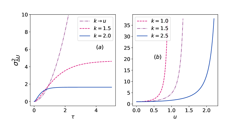
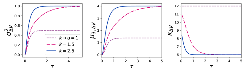
This expression is similar to Eq. 20. It is the square of the individual terms of Eq. 20. Therefore, it is also monotonically increasing in time, as we can see by 2a) which shows the temporal evolution of variance for different values of . Notably, as approaches , we observe a divergence, similar to that of the average.
Following the divergent behavior of the limit of , the variance does not have an asymptotic limit in this regime. As one can see by
| (24) |
This outcome is expected because, in that limit, the particle is in a saddle-point potential, (as depicted in 1a). The incapability of the particle to reach equilibrium arises from the non-confining regime.
As for values of , the obtained variance saturates at long times. This behavior is easy to understand by considering the asymptotic limit
| (25) |
which shows the divergence for . Depicted in 1a) we can observe that for higher values of , the saturation occurs more rapidly, which is logical since the confinement is stronger.
Analyzing the variation of with in the asymptotic limit, Eq.25, in 2b), one can observe that varies positively with , and this happens due to the growth of fluctuations from coupling between positions. Furthermore, by looking at 2a), notice that as increases, the growth of with is suppressed. Such behavior can also be observed for very large values of , where the variance in the asymptotic limit becomes constant, that is
| (26) |
where represents the asymptotic equality for larger values of .
The next quantities - skewness, and excess kurtosis - can be expressed analytically, with their analytical forms presented on C. Since the expressions are long and complicated, we adopt a graphical analysis to explore and interpret these statistical measures.
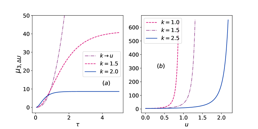
By means of the skewness, we measure the asymmetry of the distribution. Its formula is written in Eq.78. Remembering that the initial distribution of positions is a delta centered at the origin, we will only have positive values for the harmonic contribution. Therefore, the skewness will always be positive, growing monotonically over time, as can be seen in 3 a). In 3 for , we observe that the skewness evolves over time, saturating at a certain asymptotic value, which will be
| (27) |
By this formula, we also can see, that as approaches , we have a positive divergence in the skewness, a consequence of being in the non-confining regime and our skewness not being normalized. Moreover, in 3 b), we observe the behavior of with respect to for different values of in the asymptotic time regime. As we increase we increase the skewness of the harmonic potential, since this increase the fluctuations.

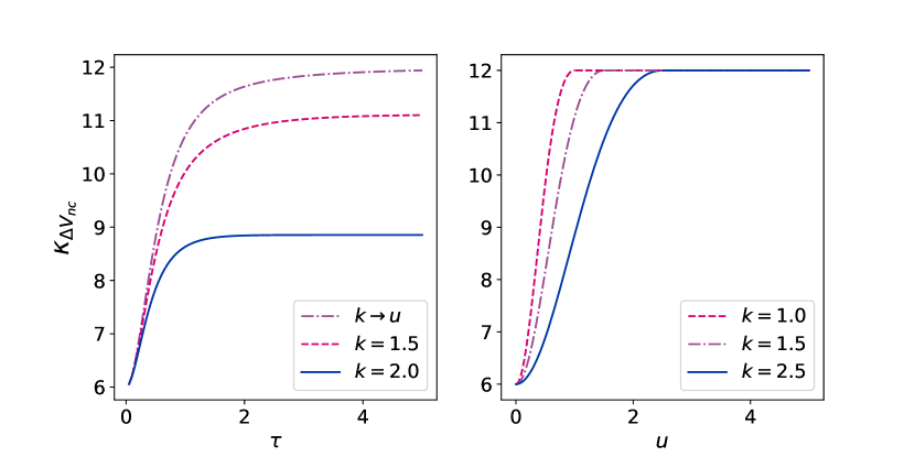
On the other hand, the excess kurtosis measures the behavior of outlier values in the distribution, particularly associated with the tails of the distribution. It is defined as the normalized fourth moment minus 3, as given by equation 83. In 4a), we present the temporal evolution of excess kurtosis, which consistently remains positive for all times, indicating that the distribution is leptokurtic. This means it has a higher probability of rare events occurring compared to a normal distribution [37]. Unlike the other quantities, we observe that kurtosis does not diverge as . This is because it is a normalized quantity, and the divergence of the fourth central moments cancels with the divergence of the variance. The asymptotic time behavior is
| (28) |
That is, for the asymptotic limit, it stabilizes at as , independently of or . Moreover, similar to the other cases, as increases, the asymptotic excess kurtosis also increases, as we can see in 4b), leading to more fluctuations in the tail of the distribution.
III.2 Distribution
The distribution is obtained by taking the Fourier transform of the characteristic function, that is
| (29) |
however, for the harmonic potential, due the signal of the coefficients, s, we cannot find an analytic expression.
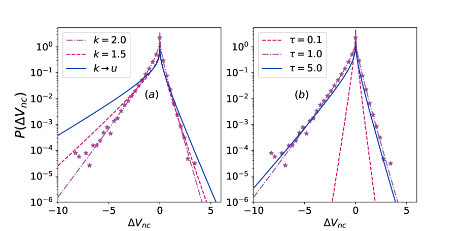
As the distribution cannot be calculated from the formula in Eq. 77, we compute it numerically and compare with numerical simulations of the Langevin equation. 5 shows in variation with for many regimes of parameters, with the purple stars being the results for the simulations of the Langevin equation. The right side depicts for different values. It admits only positive values as , as expected from the skewness. The growth of as happens in agreement with the results of 4. In 4-a, we illustrate for various values of , whereas in 4-b, we do the same for distinct values of . Since the particle is initially centered at the origin of the coordinate system, with the position probability distribution being a delta, exhibits lower kurtosis for shorter times. This is due to the initial distribution being highly concentrated around .
IV Fluctuations of the non-confining potential
Next, we calculate the fluctuations for the non-confining potential contribution. The variation can be expressed as
| (30) |
As in the previous case, to construct the characteristic function we only needs the set of coefficients, as showed in the B, represented in Eq. (73). Therefore, for the coefficients we have
| (31) | |||
| (32) | |||
| (33) |
With these coefficients we can construct the characteristic function, as showed in Eq. 73, allowing the calculation of moments and distribution.
IV.1 Central Moments
Following the previous case, we again use the characteristic function to extract the moments of the distribution of by taking derivatives of and construct the mean, variance, skewness and excess of kurtosis. As already mentioned, the average is given by the first moment, which is
| (34) |
which is remarkably similar to Eq. (20). But here, we have the coupling multiplying all the expression, and a difference of two terms, instead of a sum as in Eq. (20). When we consider , the asymptotic limit gives
| (35) |
This implies that the asymptotic limit is divergent when , similar to the behavior of . This is expected, as in the non-confining regime, the particle is not confined to a specific region, and moreover, the mean is negative. We can also derive an expression for the mean in the non-confining regime, but only for a finite transient time. This expression is as follows:
| (36) |
Note that there is also a term with linear dependence with , meaning it will negative diverge at .
The variance of will be given by
| (37) |
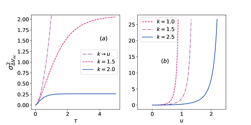
For variance, in the confining regime, we observe a monotonically increasing evolution that saturates at a plateau in the asymptotic time, reducing the rate of evolution as we increase the harmonic coupling . This increased coupling enhances confinement, limiting fluctuations, and consequently decreasing variance. However, in the non-confining regime, when , variance asymptotically diverges, as seen in the transient formula
| (38) |
which diverges for long times . Nevertheless, in the confining regime, , we have an asymptotic time behavior given by
| (39) |
Analyzing the variance in the asymptotic limit, as can be seen in 6(b), as increases and the particle becomes unbounded, we notice that the variance diverges, that is (for , it diverges as in the denominator makes an appear). Interesting, the variance of the non confining contribution has the same behavior of the harmonic contribution, we can relate both equations by as one can see by Eq. 37 and 23.

We proceed to investigate the skewness of the distribution of , given by equation 88. Again, because of the initial Dirac delta distribution, the fluctuations are asymmetric. However, different from the previous case, it is negative. Meaning the left area of the distribution is bigger than the positive. In 7, (a) illustrates the behavior of on for various values of . Our results show a negative divergence of as approaches in the non-confining regime. 7 (b) depicts the behavior of varying with for the asymptotic limit, following the expression
| (40) |
Showing that when we have a negative divergence as expected in the non-confining regime. Compared with the harmonic case, our skewness in the non-confining contribution contains smaller values. And this will be reflected in the distribution as we will see. Unlike the harmonic case, the non-confining contribution allows us to have positive and negative values in the distribution.
The excess kurtosis is equivalent to the harmonic case, as expressed in Eq. 83, and is illustrated in 8. In 8(a), we observe the variation of the excess kurtosis with respect to , demonstrating that this distribution is also leptokurtic. And is monotonic increasing in time. Furthermore, it remains finite as approaches , stabilizing at a specific value in the asymptotic limit as . This is a consequence of it being the normalized fourth moment.
In 8(b), we display the variation of the excess kurtosis with in the asymptotic limit, which is given by
| (41) |
demonstrating that it stabilizes with the growth of as . Having analyzed the most significant central moments, it becomes evident that the even moments (kurtosis and variance) are closely related to the harmonic case, revealing similarities between these two distinct quantities.
IV.2 Distribution
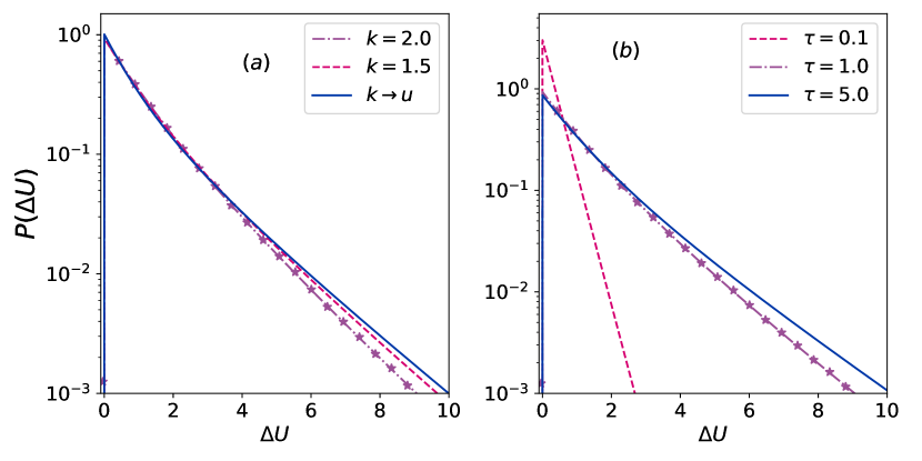
Since for the non-confining contribution, , the coefficient is positive, we are able to find a analytic expression for the distribution (See Eq. (77) in the B). It is given by
| (42) |
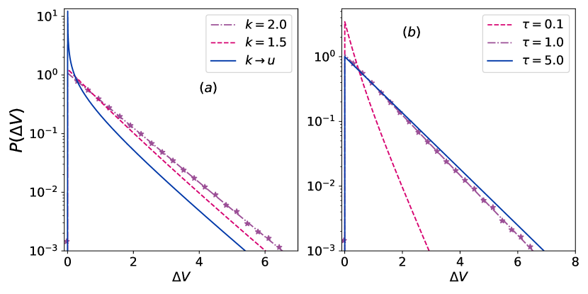
9 depicts the probability distribution varying with for many regimes of parameters given by eq. (42), with the purple stars being the results for the simulations of the Langevin equation. The right side depicts for many values. Being the distribution proportional to , it will diverge for , which is usual for Bessel type distributions [10, 16], for instance another distribution having this behavior is a Dirac delta distribution. This divergence does not affect the normalization of the distribution.
Aside from this point, the tails and width of grow as , in agreement with the behavior of the excess of kurtosis and the variance. This left side of the distribution increases, while the right side decreases, as expected from the skewness. Moreover, in 9 b), one can observe in variation with for different values of . The behavior is in agreement with the predictions from the central moments.
In the non-confining regime, the distribution obeys a relation analogous to the Fluctuation theorem [38]. By calculating the log ratio between the distribution of and its reverse process, given by distribution , one gets
| (43) |
Now considering for the non-confining regime , it becomes
| (44) |
and for a asymptotic time we have
| (45) |
Which is a Ratio of Irreversibility (RI) [39]. This RI is a mathematical consequence of the expression for that admits proportional probabilities for both and . Even though it is similar to Crooks fluctuation theorem [40], as far as we know, it does not necessarily has any physical relation to it, being a mathematical consequence of the non-confining contribution and the behavior of the dynamics in the non-confining regime.
V Fluctuations of the full potential
Finally, having investigated the two contributions of the total potential. We proceed to investigate the full variation of potential energy, that can be expressed as:
| (46) |
Again, as introduced in the previous sections, we only need set of coefficients, which comes from the fact that the potential is quadratic and the positions are Gaussian variables.
Thus, the coefficients of the characteristic function, Eq. 73, are given by:
| (47) | |||
| (48) | |||
| (49) |
Having the characteristic function, we proceed to calculate the central moments.
V.1 Central Moments
The mean is given by
| (50) |
which comes from the summation . Note that the dependence on the coupling constant, only appear in the function . Different from the previous case, there is no divergence, even in the non-confining regime in the asymptotic time limit, that is
| (51) |
Note that the mean becomes proportional to the temperature, and a lower temperature for the non-confining regime. It is similar to the equipartition theorem [41], meaning that the non-confining regime has lower energy than the confining case.
The variance of the full potential is analogous, and can be expressed as
| (52) |
For values , similarly to the cases of and , the variance of the total energy saturates at long times, even for values of in the limit . This can be understood as, in the limit of asymptotic time, one gets
| (53) |
without any dependency on and . As expected since we are in the asymptotic time. Similar to the mean, we also observe a lower value in the non-confining regime. In 10 (a), the temporal evolution of the variance of for different values of is depicted. It’s evident that, apart from the stabilization of in the asymptotic time regime, the magnitude of varies with changes in Notably, as approaches , the saturation occurs at a lower value compared to the confining case, where a higher results in a faster evolution towards the asymptotic time.
As for the skewness we have a more compact formula compared with the previous cases, we have
| (54) |
where in 10 b) depicts the temporal evolution of the skewness , for different values of . Following a similar tendency to the variance, the skewness saturates faster with . And for the asymptotic limit, we have
| (55) |
We again, do not have a divergence in the non-confining regime. What’s happens is that the for the skewness becomes
| (56) |
which does not diverge for .
Now, for the excess of kurtosis, we have a long expression, written in Eq. 93. 10 c) depicts the temporal evolution of the excess of kurtosis for different values of with set to one. we see that, for , it decreases with , saturating close to for stronger values of . At the non-confining regime, the kurtosis is constant for all times. Its asymptotic limit, is given by
| (57) |
This demonstrates that the kurtosis is constant and positive for both regimes. Thus, Leptokurtic. Like the previous moments, it exhibits no dependence on temperature. It’s worth noting that this is the case because we are dealing with the normalized fourth central moment, which is dimensionless.
V.2 Distribution
In a similar fashion to the harmonic case, it is not possible to obtain the distribution from equation 77. We then proceed to determine numerically the distribution, and compare to the numerical simulations of the Langevin equation.
11 a) depicts the probability distribution in variation of for different values of , with the purple stars being the results for the simulations of the Langevin equation. All distributions are completely asymmetric due to for all values of and , even in the non-confining regime .
The time evolution of the distribution is showed in 11 b), for many values. It is in agreement with the expected behavior of the central moments, as we see that the distribution becomes broader and skew as predicted by the variance and kurtosis. Besides that, the distribution tail increases compared with the initial time value, as expected from the excess of kurtosis.
While for the non-confining potential our results show the existence of a RI, reported in Eq. 45, for the full potential the scenario is different. As one can see clearly from the fact that the distribution admits only positives values. Nevertheless, we can discuss what is happening. For instance, let us consider the full potential difference
| (58) |
Considering the particle at the origin of the coordinates system (in a delta distribution), meaning , one has
| (59) |
For the RI, one consider the non-confining regime of the potential . That is, for any pair , one gets
| (60) |
From this result, we must know that the system does not admit regimes of . That means that the probability for . Then, for the fluctuation theorem one has
| (61) |
The same discussion applies to the harmonic case as well.
VI Discussion and conclusion
We investigated the fluctuations of a quadratic potential associated to a Brownian particle in a parabolic trap, which exhibits two regimes: confining and non-confining. These fluctuations are inherent to the system, that consists of a Brownian particle in two dimensions, with motion starting at the origin.
We divided the total potential into two contributions: a harmonic one, which is confining, and another non-confining one. We explored the fluctuations of each contribution in both regimes, confining and non-confining. We found that the even central moments (variance and kurtosis) are qualitatively similar, despite the odd moments (mean and skewness) having opposite signs. In the non-confining regime, except for the excess kurtosis, all statistical quantities are observed to diverge in the asymptotic time limit. This is a characteristic of the system, since the position distribution becomes unbounded in this regime, approaching a zero distribution in the asymptotic time limit.
For the total potential, the behavior is different; all quantities remain finite in any regime in the asymptotic limit. Additionally, we observe the emergence of the equipartition of energy theorem, as the potential becomes , with for the non-confining regime () and for the confining regime. We can interpret this as follows: In the confining regime, , we have two potentials, the harmonic one, , and the non-confining contribution, , resulting in a greater degree of freedom compared to the non-confining regime, where the potential becomes a single term, , contributing to only one degree of freedom.
In addition to the moments, we also computed the distributions and compared the results with numerical simulations, finding agreement. Due to the presence of negative coefficients in the characteristic function, obtaining an analytical expression for the harmonic contribution and the total potential is not feasible. In both cases, we have completely positive distributions due to the initial Dirac delta condition for positions.
However, for the non-confining contribution, the result is analytical and provides an asymmetric Bessel-type distribution, where the asymmetry arises from the exponential multiplied by the Bessel function. Unlike the other cases, this distribution allows for both positive and negative values. This enables the analysis of the irreversibility ratio, where we find an expression similar to Crooks’ fluctuation theorem [42]. It’s essential to emphasize that this similarity is purely a mathematical consequence of the form of this potential.
In this article, we focused on the potential energy fluctuations over a time interval and its individual contributions. It is worth noting that the behavior discussed here can be used to interpret heat, which, for the studied system, differs from the potential difference due to kinetic energy, i.e., (even in the overdamped regime, as pointed out in [15]). Therefore, our work not only investigates potential fluctuations in different regimes but could also contribute to the understanding of another quantities in stochastic thermodynamics.
Furthermore, possible generalizations of this work are feasible. A situation of interest is to consider different thermal baths, each coupled to a degree of freedom, leading to a non-equilibrium steady state (NESS), as usually discussed on the context of Brownian Gyrators.
Acknowledgments
This work is supported by the Brazilian agencies CNPq, CAPES, and FAPERJ. This study was financed in part by Coordenação de Aperfeiçoamento de Pessoal de Nível Superior—Brasil (CAPES)—Finance Code 001.
Appendix A Path Integrals Calculation
In the action formula, the conditional probability is given by
| (62) |
As the action is quadratic, therefore we just need to calculate the extremized action, and the result will be
| (63) |
The action represents the action evaluated at the solution of the Euler-Lagrange equations for the space coordinates, that gives the deterministic path. It is given by:
| (64) | |||
| (65) |
Solving both equations with boundary conditions , , and , one gets the solutions
| (66) | |||
| (67) |
Adopting the delta initial condition and , the extremized path reduces to
| (68) | |||
| (69) |
From the extremal path , one can straightforwardly calculate the Lagrangian for the extremal path, and from it, determine the action for the extremal path. For the general case with and , the action for the extremal path is given by
| (70) |
and with delta initial condition it reduces to
| (71) |
With the action on the extreme path, one can calculate the conditional probability, given by
| (72) |
Appendix B Characteristic Function and Distribution
We are interested in investigating the fluctuations of the harmonic potential and the full potential. One thing we can notice is that since both quantities have a quadratic dependence on the positions, the characteristic function will be of the type
| (73) |
With this, we can calculate all moments of the distribution by
| (74) |
These result comes from the integral
| (75) |
since is a Gaussian distribution together with the chosen initial conditions which is the zero entropy condition, and is the quadratic functional dependence on the positions. What will change will be the coefficients ’s, depending on the structure of the potential. Nevertheless, we can calculate the Fourier transform of this characteristic function, giving the distribution. We need to notice that we have:
| (76) |
where, for , we complete the square in the denominator to find this Bessel function definition [10, 16]. Performing the integral, we have:
| (77) |
where is the quantity of interest, which can be either the difference in the harmonic potential or the difference in the full potential . This formula only holds for distributions with . For distributions with , one has to calculate the distribution numerically. We will see that, despite the similarity between the two quantities and having the same distribution, the statistical behavior of the moments is different.
Appendix C Skewness and kurtosis for the potentials
The skewness and kurtosis can be expressed analytically, for all potentials fluctuations. Here we show its long and complicated formulas.
C.1 Harmonic potential
For the harmonic potential , the equation for is given by
| (78) |
where
| (79) | |||
| (80) | |||
| (81) | |||
| (82) |
The kurtosis is given by
| (83) |
with
| (84) | |||
| (85) | |||
| (86) | |||
| (87) |
C.2 Non-confining potential
For the non-confining potential , the equation for the skewness is given by
| (88) |
with
| (89) | |||
| (90) | |||
| (91) | |||
| (92) |
The equation for the excess of the kurtosis, as already mentioned in the text, is equal to the harmonic case, that is, Eq. 83, with the same coefficients.
C.3 Total potential
For the total potential, the skewness is not long and complicated, so we only insert the excess of kurtosis here. It is given by
| (93) |
where
| (94) | |||
| (95) |
References
- [1] Sekimoto K 2010 Stochastic energetics
- [2] Tomé T and De Oliveira M J 2015 Stochastic dynamics and irreversibility (Springer)
- [3] de Oliveira M J 2020 Revista Brasileira de Ensino de Física 42 e20200210 ISSN 1806-1117 URL https://doi.org/10.1590/1806-9126-RBEF-2020-0210
- [4] Peliti L and Pigolotti S 2021 Stochastic Thermodynamics: An Introduction (Princeton University Press)
- [5] Salazar D S and Lira S A 2019 Physical Review E 99 062119
- [6] Salazar D S 2020 Physical Review E 101 030101
- [7] Colmenares P J and Paredes-Altuve O 2021 Physical Review E 104 034115
- [8] Colmenares P J 2022 Physical Review E 105 044109
- [9] Chatterjee D and Cherayil B J 2011 Journal of Statistical Mechanics: Theory and Experiment 2011 P03010
- [10] Chatterjee D and Cherayil B J 2010 Physical Review E 82 051104
- [11] Saha B and Mukherji S 2014 Journal of Statistical Mechanics: Theory and Experiment 2014 P08014
- [12] Pires L B, Goerlich R, da Fonseca A L, Debiossac M, Hervieux P A, Manfredi G and Genet C 2023 Phys. Rev. Lett. 131(9) 097101
- [13] Paraguassú P V, Defaveri L and Morgado W A 2023 The European Physical Journal B 96 22
- [14] Paraguassú P V and Morgado W A M 2021 Journal of Statistical Mechanics: Theory and Experiment 2021 023205 URL https://dx.doi.org/10.1088/1742-5468/abda25
- [15] Paraguassú P V, Aquino R, Defaveri L and Morgado W A 2022 Physical Review E 106 044106
- [16] Paraguassú P V, Aquino R and Morgado W A 2023 Physica A: Statistical Mechanics and its Applications 615 128568
- [17] Darabi F, Ferrer B R and Gomez Solano J R 2023 New Journal of Physics
- [18] Gomez-Solano J R 2021 Frontiers in Physics 9 643333
- [19] Imparato A, Jop P, Petrosyan A and Ciliberto S 2008 Journal of Statistical Mechanics: Theory and Experiment 2008 P10017
- [20] Joubaud S, Garnier N and Ciliberto S 2007 Journal of Statistical Mechanics: Theory and Experiment 2007 P09018
- [21] Ciliberto S 2017 Physical Review X 7 021051
- [22] Filliger R and Reimann P 2007 Phys. Rev. Lett. 99(23) 230602 URL https://link.aps.org/doi/10.1103/PhysRevLett.99.230602
- [23] Argun A, Soni J, Dabelow L, Bo S, Pesce G, Eichhorn R and Volpe G 2017 Phys. Rev. E 96(5) 052106
- [24] Mancois V, Marcos B, Viot P and Wilkowski D 2018 Phys. Rev. E 97(5) 052121 URL https://link.aps.org/doi/10.1103/PhysRevE.97.052121
- [25] dos S Nascimento E and Morgado W A 2021 Journal of Statistical Mechanics: Theory and Experiment 2021 013301
- [26] van Kampen N G 2007 Stochastic Processes in Physics and Chemistry 3rd ed (Elsevier)
- [27] Farago O 2021 Phys. Rev. E 104(1) 014105
- [28] Streißnig C and Kantz H 2021 Physical Review Research 3 013115
- [29] Guarnieri F, Moon W and Wettlaufer J 2017 Journal of mathematical physics 58
- [30] Ryabov A, Dierl M, Chvosta P, Einax M and Maass P 2013 Journal of Physics A: Mathematical and Theoretical 46 075002
- [31] Aghion E, Kessler D A and Barkai E 2019 Phys. Rev. Lett. 122(1) 010601 URL https://link.aps.org/doi/10.1103/PhysRevLett.122.010601
- [32] Aghion E, Kessler D A and Barkai E 2020 Chaos, Solitons & Fractals 138 109890 ISSN 0960-0779 URL https://www.sciencedirect.com/science/article/pii/S0960077920302903
- [33] Defaveri L, Anteneodo C, Kessler D A and Barkai E 2020 Phys. Rev. Res. 2(4) 043088 URL https://link.aps.org/doi/10.1103/PhysRevResearch.2.043088
- [34] Wio H S 2013 Path Integrals for Stochastic Processes (WORLD SCIENTIFIC) (Preprint eprint https://www.worldscientific.com/doi/pdf/10.1142/8695) URL https://www.worldscientific.com/doi/abs/10.1142/8695
- [35] Brandão I, Tandeitnik D and Guerreiro T 2021 Quantum Science and Technology 6 045013
- [36] Ranfagni A, Vezio P, Calamai M, Chowdhury A, Marino F and Marin F 2021 Nature Physics 17 1120–1124
- [37] Darlington R B 1970 The American Statistician 24 19–22
- [38] Seifert U 2012 Reports on progress in physics 75 126001
- [39] Evans D J and Searles D J 2002 Advances in Physics 51 1529–1585
- [40] Crooks G E 1999 Physical Review E 60 2721
- [41] Jackson E A 2000 Equilibrium statistical mechanics (Courier Corporation)
- [42] Crooks G E 2000 Physical Review E 61 2361