Physics-informed laboratory estimation of Sargassum windage

Abstract

A recent Maxey–Riley theory for Sargassum raft motion, which models a raft as a network of elastically interacting finite-size, buoyant particles, predicts the carrying flow velocity to be given by the weighted sum of the water and air velocities $(1-\alpha)\mathbf{v}+\alpha\mathbf{w}$. The theory provides a closed formula for parameter $\alpha$, referred to as windage, depending on water-to-particle-density ratio or buoyancy ($\delta$). From a series of laboratory experiments in an air–water stream flume facility under controlled conditions, we estimate $\alpha$ ranging from 0.02 to 0.96%. On average, our windage estimates can be up to 9 times smaller than considered in conventional Sargassum raft transport modeling, wherein it is customary to add a fraction of $\mathbf{w}$ to $\mathbf{v}$ chosen in an ad-hoc piecemeal manner. Using the formula provided by the Maxey–Riley theory, we estimate $\delta$ ranging from 1.00 to 1.49. This is consistent with direct $\delta$ measurements, ranging from 0.9 to 1.25, which provide support for our $\alpha$ estimation.

Pelagic Sargassum has been known to be abundant throughout the North Atlantic, particularly the western end of the subtropical gyre, known as the Sargasso Sea. Forming rafts, these brown algae serve as an important habitat for ecologically and economically important marine fauna (Bertola et al., 2020). Intriguingly, since 2009 the equatorial Atlantic has emerged as a new region of extreme Sargassum abundance (Wang et al., 2019; Addico and deGraft Johnson, 2016). Pelagic Sargassum has since seasonally inundated the coasts of the Caribbean Sea, Gulf of Mexico, South Florida, northern Brazil, and western Africa. Representing a new form of coastal hazard, Sargassum inundations have direct impacts on the water quality, nearshore ecosystems, and the local economies (Smetacek and Zingone, 2013). Predicting the locations and severity of coastal inundations of pelagic Sargassum is a challenging problem.

The challenge stems in large part from the fact that a Sargassum raft’s motion is fundamentally unlike Lagrangian (i.e., infinitesimally small, neutrally buoyant) particle motion since it is a finite-size and buoyant object subjected to the action of ocean currents and winds mediated by inertia effects (Beron-Vera, 2021).

The de-jure fluid mechanics model for describing such effects is provided by the Maxey–Riley equation (Maxey and Riley, 1983). This equation is a Newton-type equation with forces (mainly flow, added mass, and drag) that affect the motion of small, spherical “inertial” particles immersed in the flow of a fluid (Cartwright et al., 2010). For particles floating at the ocean surface a Maxey–Riley equation has been recently proposed by Beron-Vera, Olascoaga, and Miron (2019). The equation, referred to herein as the BOM equation, was verified in the field (Olascoaga et al., 2020; Miron et al., 2020a) and under controlled laboratory conditions (Miron et al., 2020b). One aspect, among several others including Earth rotation effects, that makes the BOM equation different than the Maxey–Riley equation is that the carrying flow velocity is given by

$$\mathbf{u}(\mathbf{x},t)\coloneqq(1-\alpha)\mathbf{v}(\mathbf{x},t)+\alpha\mathbf{w}(\mathbf{x},t).$$ (1)

Here, $\mathbf{v}(\mathbf{x},t)$ and $\mathbf{w}(\mathbf{x},t)$ ($\mathbf{x}$ and $t$ denote horizontal position and time, respectively) are water and air velocities near the water surface, respectively, and $\alpha\in[0,1)$ is a coefficient that depends in closed form on the water-to-particle-density ratio, which we denote by $\delta$ and call buoyancy (the reserve volume is $1-\delta^{-1}$) (cf. Appendix A). We call $\alpha$ itself the windage; it is a fractional measure of the overall contribution of wind to the carrying flow velocity in the BOM equation.

Buoyancy-dependent windage $\alpha(\delta)$ has been identified as the most important factor controlling isolated object drift at the ocean surface (Olascoaga et al., 2020; Miron et al., 2020a) and can be expected to have a similarly influential role in Sargassum raft drift. In this note we seek to frame Sargassum windage in the laboratory under controlled conditions by building on the BOM model.

The BOM equation, however, cannot be expected to describe Sargassum raft motion. A Maxey–Riley model for the drift of Sargassum rafts was proposed by Beron-Vera and Miron (2020) based on the BOM equation by envisioning them as networks of elastically interacting inertial particles. The gas-filled bladders that keep a raft afloat represent the inertial particles in the proposed model, herein referred to as the eBOM model, and the flexible stems that connect them are substituted by massless springs. While the eBOM model still requires quantitative testing against observations, it has been successful in qualitatively explaining transport of Sargassum and coastal inundation in the Caribbean Sea (Andrade-Canto et al., 2022).

The eBOM model is a second-order system of ordinary differential equations coupled by the linear-elastic spring forces acting between adjacent particles of the network. It is assumed that each particle and spring is identical. However, in the nonrotating case with constant $\mathbf{v}$ and $\mathbf{w}$, and hence $\mathbf{u}$ in Eq. (1), the motion of the $i$th inertial particle of an elastically interacting network, i.e., a Sargassum raft, obeys

$$\ddot{}\mathbf{x}_{i}=\tau^{-1}(\mathbf{u}-\dot{}\mathbf{x}_{i}),$$ (2)

where $\tau$, proportional to the particle radius squared, is the Stokes time, measuring the inertial response time of the particle to the two-component water–air medium (cf. Appendix A). The assumption of constant $\mathbf{u}$ removes all of its time derivatives from the eBOM model, but the spring forces between particles still remain. However, Eq. (2) is possible since the elastic forces acting on the $i$th particle will vanish for all $t$ so long as it is initially separated from its neighbors by a distance equal to the natural length of the connecting springs. This suggests that, in this special case and with the appropriate initial conditions, Sargassum raft windage can be estimated from measurements of raft velocity $\mathbf{v}_{i}\coloneqq\dot{}\mathbf{x}_{i}$, satisfying

$$\mathbf{v}_{i}(t)=(\mathbf{v}_{i}(0)-\mathbf{u})\exp(-t/\tau)+\mathbf{u}.$$ (3)

Indeed, if $\mathbf{v}_{i}(0)=\mathbf{u}$ then $\mathbf{v}_{i}(t)=\mathbf{u}$ for all $t$, allowing one to estimate $\alpha$ from measurements of $\mathbf{v}_{i}$ given $\mathbf{v}$ and $\mathbf{w}$ using (1). (We take the opportunity to correct a mistake incurred in Miron et al. (2020b): Eq. (2), there, must be replaced by Eq. (3), here, with $i$ replaced by p, and “was negligible” in the 2nd para. of the left col. in p. 3 must read “can be expected to be close to the carrying flow speed.”) Below we report Sargassum windage estimates obtained from a series of laboratory experiments where the Sargassum raft velocity was measured as rafts drifted in a flume with constant water velocity and air streams of varied intensities.

The laboratory experiments were carried out in the Air–Sea Interaction Salt–water Tank (ASIST) of the Alfred G. Glassell, Jr. SUrge STructure Atmosphere INteraction (SUSTAIN) facility of the University of Miami’s Rosenstiel School of Marine, Atmospheric, and Earth Science (https://sustain.rsmas.miami.edu/) (Fig. 1). ASIST allows to control the water stream with a pump and the air stream with a fan. The acrylic ASIST flume is 15-m long, with a cross section of 1 m $\times$ 1 m. In our experiments, the flume was filled with seawater, of density 1.020 gr cm^-3, up to reaching a (mean) depth of 0.43 m. The flume bottom included a gentle slope at the head to damp wave reflection.

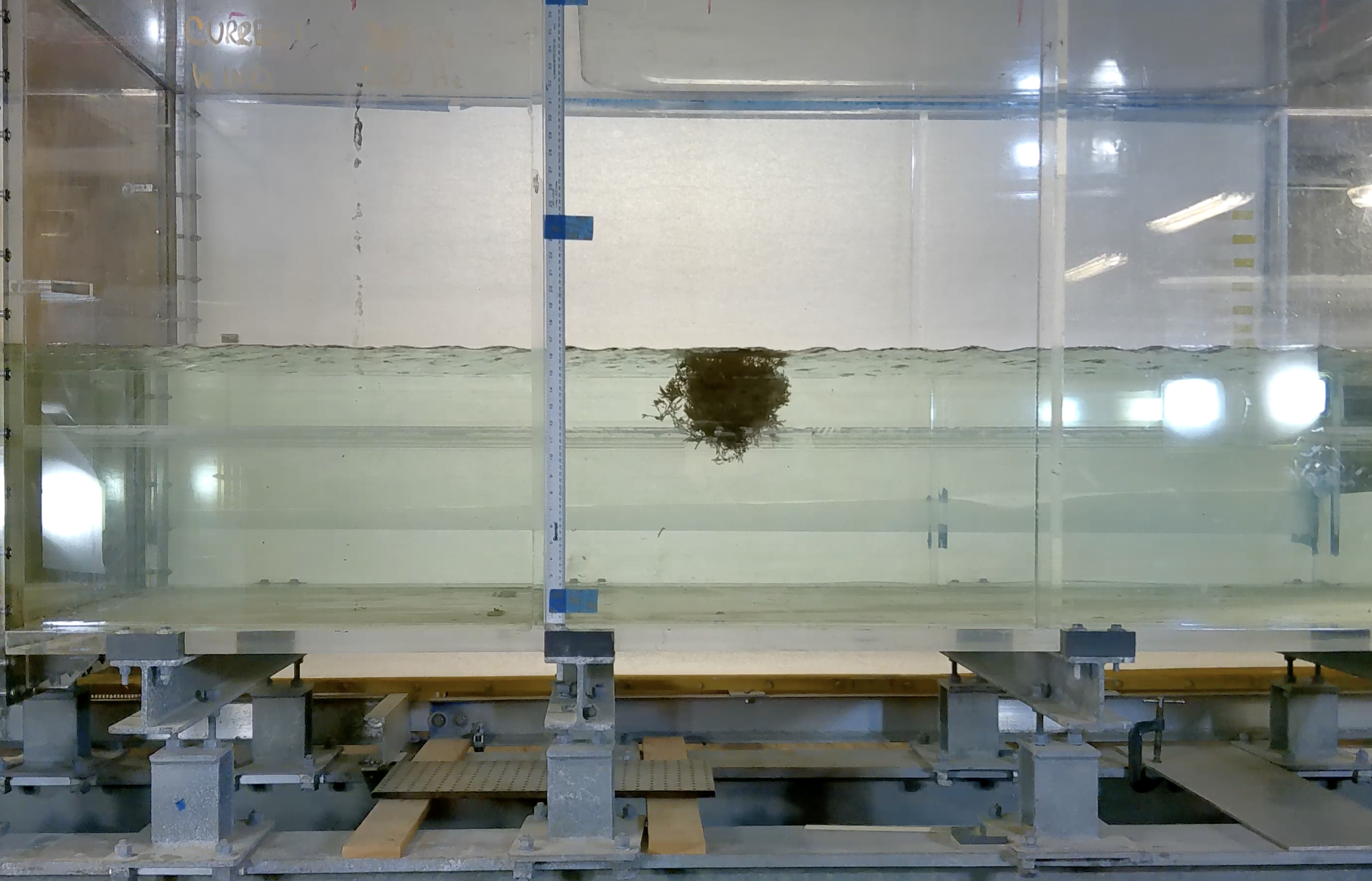
Figure 1: Side view of the ASIST air–water stream flume where the Sargassum windage experiments were carried out. A Sargassum cluster, representative of those employed in the experiments, is shown floating at the water level. The clusters used were composed of clumps collected from a raft found in the Florida Current off the southeastern coast of the Florida Peninsula.

Clumps, i.e., individual plants, of Sargassum were collected in the Florida Current off the southeastern coast of the Florida Peninsula from a small raft, with a horizontal areal coverage of about 0.5 m $\times$ 0.5 m and thickness of approximately 10 cm. Only a small portion of the raft was above water at the time of collection. The collected Sargassum clumps belonged to various species, mainly Fluitans and Natans I and VII. We estimated the density of several clusters formed by a group of clumps selected at random. Each cluster was weighted and its volume computed from the displaced volume using graduated cylinders of two different sizes. The dots in Fig. 2 are the $\delta$ values estimated for the clusters, ranging approximately from 0.91 to 1.25. The accompanying error bars are obtained by propagating the mass and volume measurement errors while ignoring those associated with the seawater density, using the standard formula which treats them as independent and random.(Ripa, 2002) The mass measurement error was 0.1 gr, while those of the volume were 1 and 5 ml when made using the smaller and larger cylinder, respectively. Performing a least squares fit of the data to a constant, we obtained $\delta=1.03\pm 0.02$. This followed by minimizing the weighted sum of the residuals squared with the weights given by the inverse of the data errors, representing our confidence on the data, and then assuming that the data had errors which were independent and random.(Ripa, 2002) The result is a weighted mean with an uncertainty given by the weighted standard deviation of the data divided by the square root of the number of data minus one, the fit’s degrees of freedom. We apply a similar procedure below, loosely referring to it as an error propagation procedure. The result that $\delta\gtrapprox 1$ is consistent with the visual observation that most clumps were at the ocean water level at the time of collection.

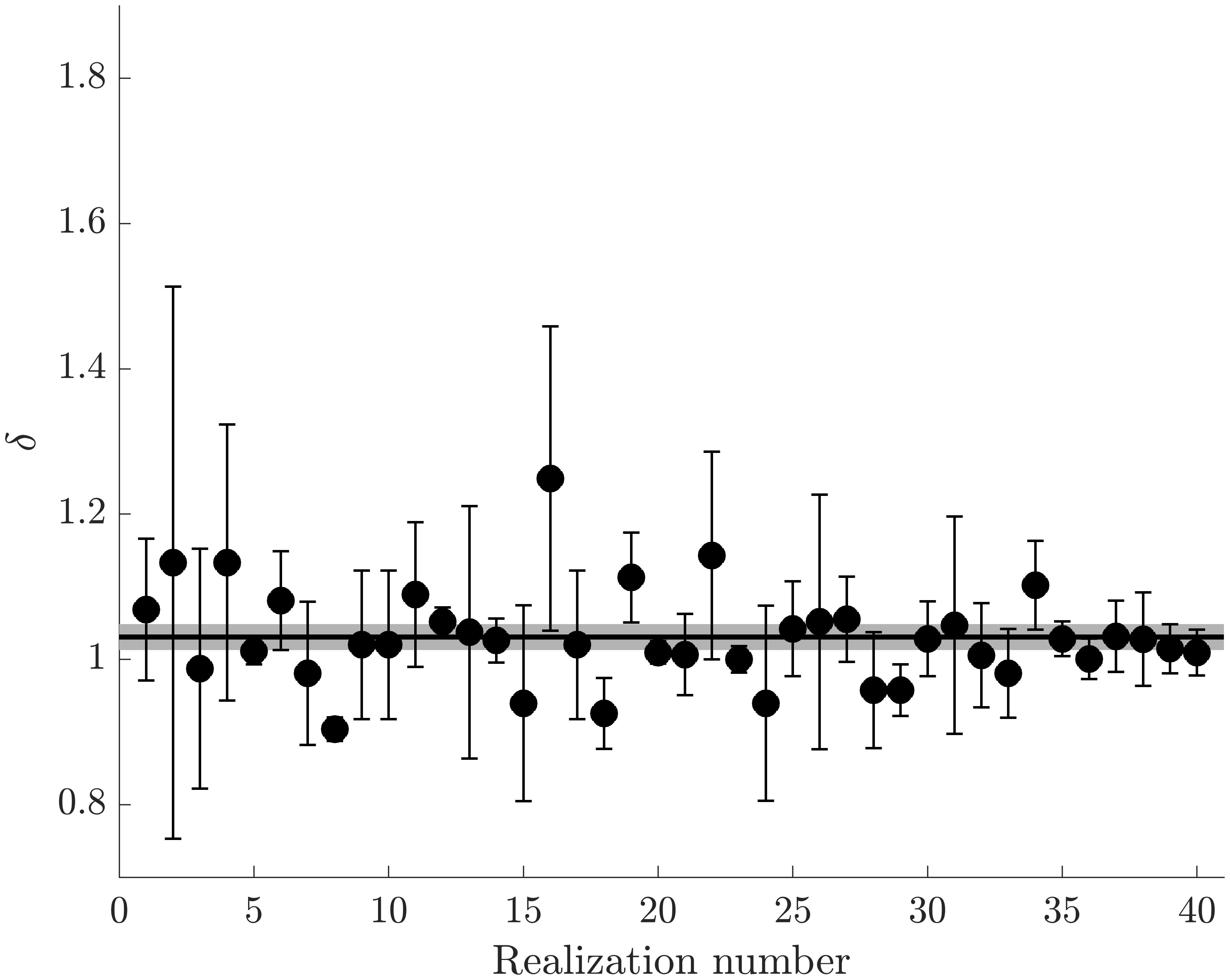
Figure 2: For each cluster of Sargassum formed by a group of clumps chose at random, a dot represents a buoyancy estimate obtained by measuring the mass and volume of the cluster. The accompanying error bar is the result of propagating the mass and volume measurement errors. The thick horizontal line is the weighted average of the individual $\delta$ estimates, where the surrounding shade represents a one-standard-deviation uncertainty.

Five fan frequencies were considered in the ASIST flume experiments, 15, 20, 25, 30, and 35 Hz. These correspond (Novelli et al., 2017) to air stream speeds (extrapolated to the mean water level from measurements roughly 0.3 m above using bulk formulas (Smith, 1988; Hsu, Meindl, and Gilhousen, 1994)) of approximately 410, 580, 760, 950 and 1150 cm s^-1, respectively. The resulting air stream speeds produced negligible to small ripples at the air–water interface, except for the highest two, which led to higher amplitude waves possibly inducing drift. The water pump frequency was set to 30 Hz. Due to friction with the walls and bottom, and the stress applied by the air stream at the surface, the resulting water stream is necessarily sheared, mainly in the vertical. Intensification of the water stream toward the surface depends on the intensity of the air stream. This was observed from particle image velocimetry (PIV) by Novelli et al. (2017) in an experimental setup that we followed as closely as possible. An effective water stream speed, depending on the air stream speed in each experiment conducted, was obtained by vertically averaging over the Sargassum cluster submerged depth the velocity profile inferred from PIV. Novelli et al. (2017) note that PIV measurements are not reliable within the top 5 cm of the water column; extrapolated values by Novelli et al. (2017) in that layer were not taken into account. We have not considered all PIV profiles reported by Novelli et al. (2017), as lack of correspondence at some depth levels with the applied air stream was noted. Thus we only considered the velocity profiles resulting at the lowest and highest air stream speeds, and linearly interpolated values at each depth for intermediate speeds. The resulting vertically averaged water stream speeds, approximately 11.6, 11.7, 12.3, 12.9, 13.5, and 14.0 cm s^-1, increase with increasing air stream speed as can be expected. In all cases the air and water stream speeds used were representative of ocean current speeds and wind intensities typically observed in the open ocean under nonrough sea conditions.

A single experiment consisted in placing a hand-size cluster of Sargassum on the water surface and allowing it to drift freely down the flume. Ten experimental realizations per air stream intensity were conducted. A few realizations were discarded in which a cluster either floated too closely to the edges of the flume or sank too far below the surface. To estimate a cluster speed, the cluster was first allowed to travel a set distance to ensure that $\mathbf{v}_{i}(0)\approx\mathbf{u}$ by Eq. (3). Then, we measured the time it took the cluster to travel a fixed length of 2.3 m using two independent chronometer measurements. We also video recorded the experiments and tracked the motion of the clusters using CSR-DCF (Discriminative Correlation Filter with Channel and Spatial Reliability) (Lukezic et al., 2018), which improves the reliability of nonrectangular object tracking. This verified the chronometer-based estimates of speed, which were largely constant during each realization. In Fig. 3 we show distance traveled by each Sargassum cluster in the along-flume direction ($\mathbf{e}$) in an experiment at fan frequency 25 Hz ($\mathbf{w}\cdot\mathbf{e}\approx 760$ cm s^-1); similar results were seen in experiments at other frequencies. This observation that $\mathbf{v}_{i}(t)$ is approximately constant allowed us to proceed to estimate Sargassum windage as proposed. Variations of speed estimates across experiment realizations were observed. Despite the care taken to ensure the drifting Sargassum avoided the walls, lateral flume boundary effects probably still existed. In addition, buoyancy variations across experiments were observed. Indeed, a tendency of the Sargassum clumps to lose bladders was noted each time a cluster was removed from the water at the end of an experiment realization to be reused in the subsequent one.

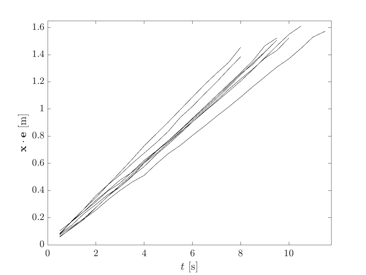
Figure 3: Distance traveled along the ASIST flume as a function of time by each Sargassum cluster in an experiment at fan frequency 25 Hz (7.6-m s^-1 air stream intensity) inferred using CSR-DCF motion tracking indicating approximately constant drift speed.

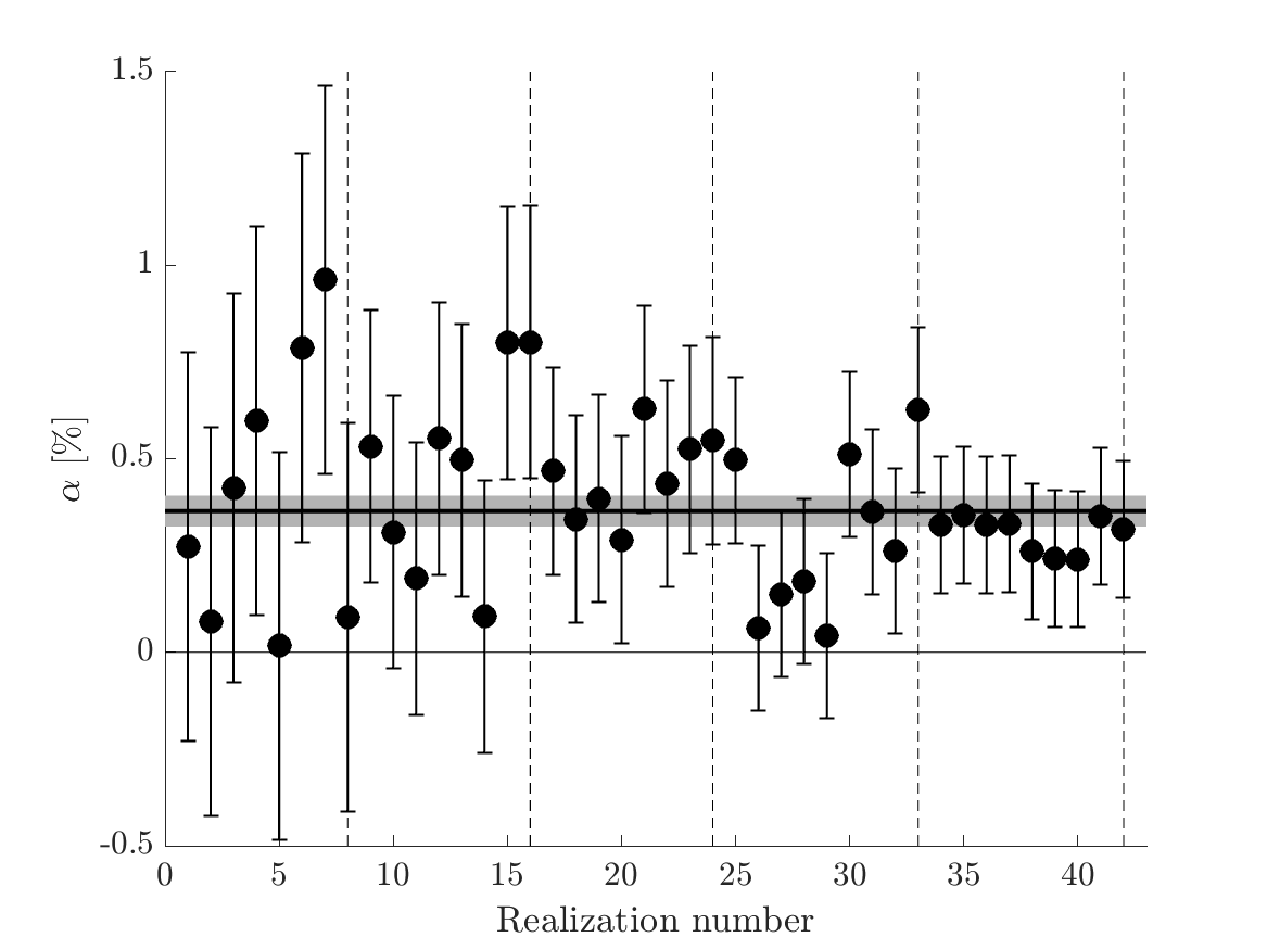
Figure 4: For each experiment realization a dot represents an estimate of the the windage ($\alpha$) parameter computed with Eq. (4) and whose error bar accounts for uncertainty in the water and wind speeds via propagation. The thick horizontal line is the weighted average of the individual $\alpha$ estimates with the corresponding uncertainty shaded around it. The dashed lines bound experiment realizations carried out at different wind speeds, increasing to the right.

Each dot in Fig. 4 is

$$\alpha=\frac{(\mathbf{v}_{i}-\mathbf{v})\cdot\mathbf{e}}{(\mathbf{w}-\mathbf{v})\cdot\mathbf{e}}$$ (4)

as estimated in a given experiment realization. The broken lines separate experiment realizations conducted at different wind speeds, increasing to the right. The error bars accompanying the estimates, ranging approximately from 0.02 to 0.96%, represent their uncertainties computed by propagating the error associated with the water and wind speeds. These are reported (Novelli et al., 2017) to be of 2 cm s^-1 and 1%  per fan frequency, respectively. The dispersion is larger for slower winds and smaller for stronger winds. Upon performing a weighted average over all individual $\alpha$ estimates we obtain $\alpha=(0.36\pm 0.04)\%$, where the uncertainty associated with the overall estimate is the result of propagating that associated with each individual estimate. The result is depicted in Fig. 4 by the thick horizontal line and accompanying shade.

The reported windage estimate are smaller than the 1–3% considered in conventional Sargassum raft transport modeling (Johns et al., 2020; Putman et al., 2020; Jouanno et al., 2021a). However, an application of the BOM model involving a Sargassum-like plastic raft tracked by satellite along with satellite-altimetry-derived ocean currents and reanalyzed near-surface winds (Olascoaga et al., 2020) appears to favor a lower windage. Indeed, the trajectory of the artificial Sargassum raft, about 2-cm thick and spanning an area of approximately 250 cm $\times$ 50 cm, was best described by the BOM model when its parameters were computed using $\delta=1.25$, corresponding to $\alpha\approx 0.5\%$. On the other hand, an analysis involving satellite-tracked trajectories of undrogued surface drifting buoys Johnson et al. (2020) favors the use of a lower windage than in conventional Sargassum modeling to improve Sargassum connectivity throughout the Tropical Atlantic and achieve a wider spread of Sargassum in the eastern Tropical Atlantic than is currently observed in satellite imagery, adhering to earlier hypotheses Franks, Johnson, and Ko (2016).

The reliability of the windage estimates can be better assessed by comparing the corresponding buoyancies with those directly inferred from Fig. 5. As noted above, both the BOM and eBOM model relate windage ($\alpha$) with buoyancy ($\delta$) in closed form. An approximate inverse relationship, $\delta(\alpha)$, appropriate for use in the near-neutrally buoyant limit, is given in Appendix A. Figure 5 shows the resulting $\delta$ estimates depending on the experiment realization, ranging from 1.00 to 1.49. The overall buoyancy estimate $\delta=1.14\pm 0.02$ lies within the range of the directly measured $\delta$, albeit toward its larger end. Differences may be attributed, in part, to the direct buoyancy measurements being made using different individual Sargassum clusters than those used during the travel time measurements (although both experiments used clusters from the same group of clumps.) This corroboration increases the confidence in the reported windage estimates and, as a consequence, the eBOM modeling framework employed to obtain them.

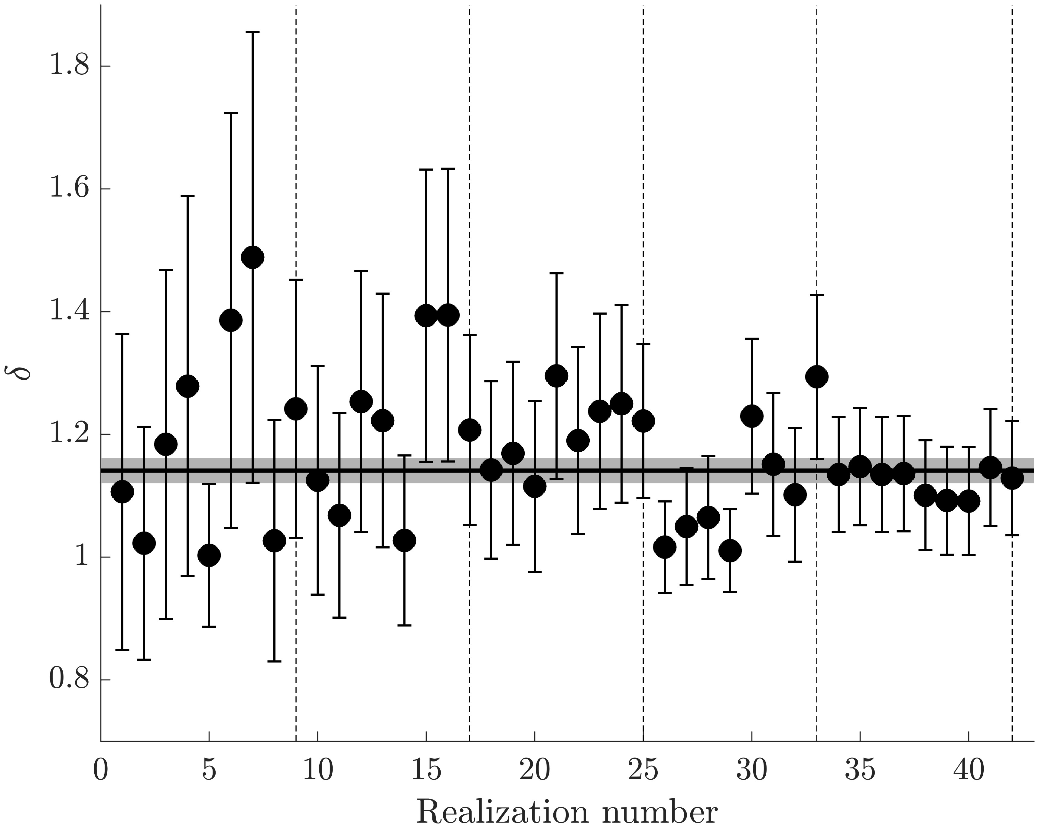
Figure 5: For each experiment realization a dot represents a buoyancy estimate computed from corresponding windage ($\alpha$) estimate as in Appendix A with an error bar obtained via propagation of the error associated with $\alpha$. The thick horizontal line is the weighted average of the individual $\delta$ estimates with the corresponding uncertainty shaded around it. As in Fig. 4, the dashed lines delimit experiment realizations carried out at different wind speeds, which increase to the right.

Our study is the first to directly measure windage of Sargassum under controlled conditions. Given the wide range of windage values used in modeling Sargassum transport, and the potential uncertainty this introduces in predictions,(Putman et al., 2018; Wang et al., 2019; Berline et al., 2020; Johns et al., 2020; Johnson et al., 2020; Jouanno et al., 2021a, b; Alleyne, Neat, and Oxenford, 2023; Podlejski et al., 2023; Lara-Hernández et al., 2024) direct measurements of wind effects on Sargassum movement are of considerable importance for predicting its movement and forecasting beaching events.(Putman et al., 2023) We expect to use the estimated windage and corresponding buoyancy values in testing the eBOM model in the field against real Sargassum raft trajectories. We have recently deployed satellite trackers in several Sargassum rafts found in the Florida Current off the southern Florida Peninsula to carry out such a test. The deployments were done in pairs so the eBOM model can be tested, approximately at least. We will report on results of the test elsewhere.

Author declarations

Conflict of interest

The authors have no conflicts to disclose.

Author contributions

Maria Olascoaga: Conceptualization (equal); Data curation (equal); Formal analysis (equal); Writing - original draft (equal); Writing - review & editing (equal). Francisco Beron-Vera: Conceptualization (equal); Formal analysis (equal); Writing - original draft (equal); Writing - review & editing (equal). Taylor Beyea: Data curation (equal); Writing - review & editing (equal). Gage Bonner: Conceptualization (equal); Formal analysis (equal); Writing - review & editing (equal). Michael Castellucci: Data curation (equal); Visualization (equal). Gustavo Goni: Resources (equal); Writing - review & editing (equal). Cedric Guigand: Resources (equal); Nathan Putman: Data curation (equal); Writing - review & editing (equal).

Data availability

Video records of the experiments are available from https://github.com/SargassumLab/SargassumWindageVideos.

Appendix A Buoyancy dependent windage and Stokes time

According to the BOM equation, the windage ($\alpha$) for spherical particle floating at the ocean–atmosphere interface varies with buoyancy ($\delta$) as

$$\alpha(\delta)=\frac{\gamma\Psi(\delta)}{1+(\gamma-1)\Psi(\delta)}.$$ (5)

Here, $\gamma$ is the air-to-water viscosity ratio,

$$\Psi(\delta)\coloneqq\pi^{-1}\operatorname{acos}\Phi(\delta)-\pi^{-1}\Phi(\delta)\smash{\sqrt{1-\Phi(\delta)^{2}}},$$ (6)

giving the fraction of emerged particle’s projected (in the flow direction) area,

$$\Phi(\delta)\coloneqq\frac{1}{2}(\varphi(\delta)^{-1}+\varphi(\delta))+\frac{\mathrm{i}\sqrt{3}}{2}\left(\varphi(\delta)-\varphi(\delta)^{-1}\right),$$ (7)

with the fraction of emerged particle piece’s height given by $1-\Phi(\delta)$, where

$$\varphi(\delta)\coloneqq\sqrt[3]{\mathrm{i}\sqrt{1-(2\delta^{-1}-1)^{2}}+2\delta^{-1}-1}.$$ (8)

Note the slight change of notation in Eq. (6) with respect to earlier references(Miron et al., 2020a, b; Beron-Vera and Miron, 2020; Beron-Vera, Olascoaga, and Miron, 2019; Olascoaga et al., 2020; Beron-Vera, 2021).

As pointed out in Olascoaga et al. (2020), the above formulae is not valid for $\delta\geq 1$ very large, which is of no consequence in general and in particular in the near-neutrally buoyant case, $\delta\approx 1$, which of interest here. We can construct a series reversion for $\delta(\Psi)$, which is accurate to $0.05\%$ or less for $1\leq\delta\lessapprox 1.5$,

$$\delta(\Psi) \sim 1$$

$$+1.481344653620955\cdot\Psi^{4/3}$$

$$-0.2775826237806382\cdot\Psi^{2}$$

$$+2.114966253909641\cdot\Psi^{8/3}$$

$$-0.8594639386944948\cdot\Psi^{10/3}$$

$$+3.071255172923317\cdot\Psi^{4}$$

$$-1.906635056270554\cdot\Psi^{14/3}$$

$$+4.589911692676772\cdot\Psi^{16/3}$$

$$-3.708388371098538\cdot\Psi^{6}.$$ (9)

Solving Eq. (5) for $\Psi(\alpha)$ and substituting the result into Eq. (9) provides an approximate formula for $\delta(\alpha)$.

Finally, the Stokes time involved in Eqs. (2)–(3) is defined by

$$\tau:=\frac{a^{2}\rho}{\mu}\cdot\frac{1-\frac{1}{6}\Phi}{\big{(}1+(\gamma-1)\Psi\big{)}\delta^{4}},$$ (10)

where $a$ is the particle radius, $\rho$ is the water density, and $\mu$ stands for viscosity.

(We note that in three references (Miron et al., 2020a, b; Beron-Vera and Miron, 2020) it has been typed $1-\gamma$ in Eqs. (5) and (10), instead of $\gamma-1$, as it must be.)

References

- Bertola et al. (2020) L. D. Bertola, J. T. Boehm, N. F. Putman, A. T. Xue, J. D. Robinson, S. Harris, C. C. Baldwin, I. Overcast, and M. J. Hickerson, “Asymmetrical gene flow in five co-distributed syngnathids explained by ocean currents and rafting propensity,” Proceedings of the Royal Society B 287, 20200657 (2020).
- Wang et al. (2019) M. Wang, C. Hu, B. Barnes, G. Mitchum, B. Lapointe, and J. P. Montoya, “The Great Atlantic Sargassum Belt,” Science 365, 83–87 (2019).
- Addico and deGraft Johnson (2016) G. N. D. Addico and K. A. A. deGraft Johnson, “Preliminary investigation into the chemical composition of the invasive brown seaweed Sargassum along the West Coast of Ghana,” African Journal of Biotechnology 15, 2184–2191 (2016).
- Smetacek and Zingone (2013) V. Smetacek and A. Zingone, “Green and golden seaweed tides on the rise,” Nature 504, 84–88 (2013).
- Beron-Vera (2021) F. J. Beron-Vera, “Nonlinear dynamics of inertial particles in the ocean: From drifters and floats to marine debris and Sargassum,” Nonlinear Dyn. 103, 1–26 (2021).
- Maxey and Riley (1983) M. R. Maxey and J. J. Riley, “Equation of motion for a small rigid sphere in a nonuniform flow,” Phys. Fluids 26, 883 (1983).
- Cartwright et al. (2010) J. H. E. Cartwright, U. Feudel, G. Károlyi, A. de Moura, O. Piro, and T. Tél, “Dynamics of finite-size particles in chaotic fluid flows. in thiel m., and j. kurths and m. romano and g. karolyi and a. moura (editors),” in Nonlinear Dynamics and Chaos: Advances and Perspectives (Springer-Verlag Berlin Heidelberg, 2010) pp. 51–87.
- Beron-Vera, Olascoaga, and Miron (2019) F. J. Beron-Vera, M. J. Olascoaga, and P. Miron, “Building a Maxey–Riley framework for surface ocean inertial particle dynamics,” Phys. Fluids 31, 096602 (2019).
- Olascoaga et al. (2020) M. J. Olascoaga, F. J. Beron-Vera, P. Miron, J. Triñanes, N. F. Putman, R. Lumpkin, and G. J. Goni, “Observation and quantification of inertial effects on the drift of floating objects at the ocean surface,” Phys. Fluids 32, 026601 (2020).
- Miron et al. (2020a) P. Miron, M. J. Olascoaga, F. J. Beron-Vera, J. Triñanes, N. F. Putman, R. Lumpkin, and G. J. Goni, “Clustering of marine-debris-and Sargassum-like drifters explained by inertial particle dynamics,” Geophys. Res. Lett. 47, e2020GL089874 (2020a).
- Miron et al. (2020b) P. Miron, S. Medina, M. J. Olascaoaga, and F. J. Beron-Vera, “Laboratory verification of a Maxey–Riley theory for inertial ocean dynamics,” Phys. Fluids 32, 071703 (2020b).
- Beron-Vera and Miron (2020) F. J. Beron-Vera and P. Miron, “A minimal Maxey–Riley model for the drift of Sargassum rafts,” J. Fluid Mech. 904, A8 (2020).
- Andrade-Canto et al. (2022) F. Andrade-Canto, F. J. Beron-Vera, G. J. Goni, D. Karrasch, M. J. Olascoaga, and J. Trinanes, “Carriers of Sargassum and mechanism for coastal inundation in the Caribbean Sea,” Phys. Fluids 34, 016602 (2022).
- Ripa (2002) P. Ripa, “Least squares data fitting,” Cienc. Mar. 28, 75–105 (2002).
- Novelli et al. (2017) G. Novelli, C. Guigand, C. Cousin, E. H. Ryan, N. J. Laxague, H. Dai, B. K. Haus, and Özgökmen, Tamay M, “A biodegradable surface drifter for ocean sampling on a massive scale,” Journal of Atmospheric and Oceanic Technology 34, 2509–2532 (2017).
- Smith (1988) S. D. Smith, “Coefficients for sea surface wind stress, heat flux, and wind profiles as a function of wind speed and temperature,” Journal of Geophysical Research: Oceans 93, 15467–15472 (1988).
- Hsu, Meindl, and Gilhousen (1994) S. A. Hsu, E. A. Meindl, and D. B. Gilhousen, “Determining the power-law wind-profile exponet under near-neutral stability conditions at sea,” J. App. Met. 33, 757–756 (1994).
- Lukezic et al. (2018) A. Lukezic, T. Vojír, L. Cehovin Zajc, J. Matas, and M. Kristan, “Discriminative correlation filter tracker with channel and spatial reliability,” International Journal of Computer Vision 126, 671–688 (2018).
- Johns et al. (2020) E. M. Johns, R. Lumpkin, N. F. Putman, R. H. Smith, F. E. Muller-Karger, D. T. Rueda-Roa, C. Hu, M. Wang, M. T. Brooks, L. J. Gramer, and F. E. Werner, “The establishment of a pelagic Sargassum population in the tropical Atlantic: Biological consequences of a basin-scale long distance dispersal event,” Progress in Oceanography 182, 102269 (2020).
- Putman et al. (2020) N. F. Putman, R. Lumpkin, M. J. Olascoaga, J. Trinanes, and G. J. Goni, “Improving transport predictions of pelagic Sargassum,” Journal of Experimental Marine Biology and Ecology 529, 151398 (2020).
- Jouanno et al. (2021a) J. Jouanno, J.-S. Moquet, L. Berline, M.-H. Radenac, W. Santini, T. Changeux, T. Thibaut, W. Podlejski, F. Ménard, J.-M. Martinez, O. Aumont, J. Sheinbaum, N. Filizola, and G. D. M. N’Kaya, “Evolution of the riverine nutrient export to the tropical atlantic over the last 15 years: is there a link with sargassum proliferation?” Environmental Research Letters 16, 034042 (2021a).
- Johnson et al. (2020) D. R. Johnson, J. S. Franks, H. A. Oxenford, and S.-A. L. Cox, “Pelagic Sargassum Prediction and Marine Connectivity in the Tropical Atlantic,” Gulf and Caribbean Research 31, GCFI20–GCFI30 (2020).
- Franks, Johnson, and Ko (2016) J. Franks, D. Johnson, and D. Ko, “Pelagic Sargassum in the tropical North Atlantic,” Gulf Caribbean Res 27, C6–11 (2016).
- Putman et al. (2018) N. F. Putman, G. J. Goni, L. J. Gramer, C. Hu, E. M. Johns, J. Trinanes, and M. Wang, “Simulating transport pathways of pelagic Sargassum from the Equatorial Atlantic into the Caribbean Sea,” Progress in Oceanography 165, 205–214 (2018).
- Berline et al. (2020) L. Berline, A. Ody, J. Jouanno, C. Chevalier, J.-M. Andre, T. Thibaut, and F. Menard, “Hindcasting the 2017 dispersal of Sargassum algae in the Tropical North Atlantic,” Marine Pollution Bulletin 158, 111431 (2020).
- Jouanno et al. (2021b) J. Jouanno, R. Benshila, L. Berline, A. Soulié, M.-H. Radenac, G. Morvan, F. Diaz, J. Sheinbaum, C. Chevalier, T. Thibaut, T. Changeux, F. Menard, S. Berthet, O. Aumont, C. Ethé, P. Nabat, and M. Mallet, “A NEMO-based model of Sargassum distribution in the tropical Atlantic: description of the model and sensitivity analysis (NEMO-Sarg1.0),” Geoscientific Model Development 14, 4069–4086 (2021b).
- Alleyne, Neat, and Oxenford (2023) K. S. Alleyne, F. Neat, and H. A. Oxenford, “An analysis of arsenic concentrations associated with Sargassum influx events in Barbados,” Marine Pollution Bulletin 192, 115064 (2023).
- Podlejski et al. (2023) W. Podlejski, L. Berline, D. Nerini, A. Doglioli, and C. Lett, “A new Sargassum drift model derived from features tracking in MODIS images,” Marine Pollution Bulletin 188, 114629 (2023).
- Lara-Hernández et al. (2024) J. Lara-Hernández, C. Enriquez, J. Zavala-Hidalgo, E. Cuevas, B. van Tussenbroek, and A. Uribe-Martínez, “Sargassum transport towards Mexican Caribbean shores: Numerical modeling for research and forecasting,” Journal of Marine Systems 241, 103923 (2024).
- Putman et al. (2023) N. F. Putman, R. T. Beyea, L. A. R. Iporac, J. Triñanes, E. G. Ackerman, M. J. Olascoaga, C. M. Appendini, J. Arriaga, L. Collado-Vides, R. Lumpkin, C. Hu, and G. Goni, “Improving satellite monitoring of coastal inundations of pelagic Sargassum algae with wind and citizen science data,” Aquatic Botany 188, 103672 (2023).