ARTEMIS: Using GANs with Multiple Discriminators to Generate Art

Abstract

We propose a novel method for generating abstract art. First an autoencoder is trained to encode and decode the style representations of images, which are extracted from source images with a pretrained VGG network. Then, the decoder component of the autoencoder is extracted and used as a generator in a GAN. The generator works with an ensemble of discriminators. Each discriminator takes different style representations of the same images, and the generator is trained to create images that create convincing style representations in order to deceive all of the generators. The generator is also trained to maximize a diversity term. The resulting images had a surreal, geometric quality. We call our approach ARTEMIS (ARTistic Encoder- Multi-Discriminators Including Self-Attention), as it uses the self-attention layers and an encoder-decoder architecture.

Introduction

The basic structure of a Generative Adversarial Network (GAN) is to train a generator to produce a realistic $x^{\prime}\in D$, for some dimensionality $D$ from a random distribution $z$, and a discriminator to label inputs $x\in D$ as real or false. Typically, the dimensionality $D$ is usually the dimensions of an image $L\times W\times 3$, where L and W are integers. However, in the style transfer and texture generation literature, an image can also be represented by its style representation, also known as a feature map. This opens the possibility of using multiple discriminators for one image, with each discriminator using a different shaped feature map extracted from the image. We used a pretrained VGG-19 model for mapping images to their feature maps, thus making this an example of transfer learning. We also implemented visual attention, so the generator could use nonlocal features.

Related Work

Style Transfer

Approaches that didn’t use neural networks, like Hertzmann (1998), which could redraw the edges in images to look painted, or Gooch et al. (2004), which could make human faces appear more cartoon-like, were usually limited in the range of styles they could apply to images. The first style transfer algorithm using deep learning was first implemented by Gatys et al. (2015). In this paper, style and content representations were extracted from images using the output of intermediate layers of a pretrained VGG-19 network. An image was optimized to minimize the distance between the gramm matrices of the generated image and the gramm matrices of the style and content representations. By adding a photorealistic regularization term to the objective function when optimizing the image, style could be transferred to a content image without losing the realism of the Luan et al. (2017). While a pretrained VGG-19 model is standard for extracting feature representations of images, work has been made to improve the utility of the lighter ResNet for extracting feature representations as well Wang et al. (2021).

Instead of optimizing an image, GAN approaches like Zhu et al. (2017) used a CycleGAN to generate stylized images, using content images as the source to the generator, expanded upon by Liu et al. (2018). Style transfer with GANs have also implemented attentional Park and Lee (2019) and residual Xu et al. (2021) components.

GANs for Image Generation

Originally introduced by Goodfellow et al. (2014), Generative Adversarial Networks (GANS), and an expansion on them, the Deep Convolutional GAN (DCGAN) Radford et al. (2015) have been used for writing text Saeed et al. (2019), composing melodies Kolokolova et al. (2020), making 3-D models Wu et al. (2018) and super-resolution Wang et al. (2018). Elgammal et al. (2017) optimized the generator to not only create convincing samples, but also to make it hard to classify generated samples to belong to a particular artistic category like baroque or impressionism. Works like Ulyanov et al. (2016); Xian et al. (2017) conditioned their GANs on sketches to generate realistic images.

Texture Generation

A texture is the ” the perceived surface quality of a work of art” Wikipedia (2022). Alternatively called style, it refers to things like the shape of lines, thickness of strokes and visual features other than the raw content of an image. Texture Generation is the process of generating new images that have unique textures, distinct from texture synthesis, which is ”from an input sample, new texture images of arbitrary size and which are perceptually equivalent to the sample” Raad et al. (2017). In addition to many traditional ways to generate unique textures Dong et al. (2020), machine learning can be used to generate new textures. Works like Li and Wand (2016), Johnson et al. (2016) and Ulyanov et al. (2016) used convolutional networks trained to minimize higher-level stylistic loss to generate novel textures. This method was advanced by Wilmot et al. (2017) via training the network to minimize histogram loss. While most work has been for flat images, Gutierrez et al. (2020) expanded texture synthesis to 3-dimensional objects, mapping each point in 3-dimensional space to a color.

Transfer Learning

Network-based transfer learning uses a model, or components of a model trained for one task to perform another task, for a new task Caruana (1994); Tan et al. (2018). Wen et al. (2019) used a pretrained VGG-19 Simonyan and Zisserman (2015) network to extract features and use them to classify mechanical data. Using a pretrained InceptionV3 network, Jignesh Chowdary et al. (2020) determined whether a human was wearing a mask or not. Espejo-Garcia et al. (2020) compared VGG and Inception for classifying weeds. The pretrained model does not need to be trained on a different dataset than the final model. For example, GANs can be improved by using pretrained layers of an autoencoder Nagpal et al. (2020) or variational autoencoder Ham et al. (2020) as part of the generator.

Visual Attention

When humans process input from a sequence or an image, we contextualize each part of the input using other parts of the input. However, we do not pay equal attention to every other part of the input Mnih et al. (2014). For a textual example, in the sentence ”Alan said he was hungry”, the word ”alan” is more useful in determining the meaning of ”he” than the word ”hungry”. For a visual example, in order to guess the location of the right eye on someones face, the most important information would be the location of the left eye, not the length of their beard. Attention, also known as Non-Locality was originally proposed for text Bahdanau et al. (2014); Luong et al. (2015), it was then applied to vision Wang et al. (2017); Vaswani et al. (2017), finding applications in medicine Guan et al. (2018), super-resolution Dai et al. (2019); Zhang et al. (2018), and image generation Gregor et al. (2015); Zhang et al. (2019).

Wasserstein GANs

In order to prevent mode collapse, Arjovsky et al. (2017) proposed the wasserstein GAN. As an alternative to gradient clipping, Gulrajani et al. (2017) introduced a gradient penalty term

Data

Preprocessing

The images used were the 80,000+ images in the WikiArt Images dataset Saleh and Elgammal (2015). Each image was cropped to be $(256\times 256\times 3)$. Images that were smaller than $(256\times 256\times 3)$ were concatenated with themselves and then cropped. Images were preprocessed by using the output of intermediate layers of a VGG-19 network pretrained on the ImageNet dataset. Only the 16 convolutional layers were used. These image style representations were usually different shapes than the original images. For example, a $(256\times 256\times 3)$ image would create a $(32\times 32\times 512)$ style representation output from the ”block4_conv1” layer.

Network

VGG Layers

Given the pretrained VGG-19 model, $VGG$, we define a set of its intermediate blocks $B$, and a set of corresponding dimensions $DIMS$ corresponding to the output of the corresponding block when the VGG network processes an image $\in\mathbb{R}^{256\times 256\times 3}$ image. For example $B=(block1\_conv1,block3\_conv1,block5\_conv1)$, and $DIMS_{B}=(\mathbb{R}^{256\times 256\times 64},\mathbb{R}^{64\times 64\times 256},\mathbb{R}^{16\times 16\times 12})$. We then use the notation $VGG(B)$ to mean the style representation outputs of each layer in $B$ when the VGG processes an image, and therefore

$$VGG_{B}:\mathbb{R}^{256\times 256\times 3}\longrightarrow DIMS_{B}$$

For example:

$$VGG_{(block1\_conv1,block5\_conv1)}:\mathbb{R}^{256\times 256\times 3}\longrightarrow$$

$$(\mathbb{R}^{256\times 256\times 64},\mathbb{R}^{16\times 16\times 12})$$

When $B$ is a singleton set, consisting of a single block, we may also write $VGG_{blockname}$ or $DIMS_{blockname}$, for example:

$$VGG_{block3\_conv1}:\mathbb{R}^{256\times 256\times 3}\longrightarrow DIMS_{block3\_conv1}$$

VGG Block	$DIM_{block}$
no block	$\mathbb{R}^{256\times 256\times 3}$
block1_conv1	$\mathbb{R}^{256\times 256\times 256}$
block2_conv1	$\mathbb{R}^{128\times 128\times 128}$
block3_conv1	$\mathbb{R}^{64\times 64\times 256}$
block4_conv1	$\mathbb{R}^{32\times 32\times 512}$
block5_conv1	$\mathbb{R}^{16\times 16\times 512}$

Table 1: VGG Layers and Dimensions

Autoencoder

The Autoencoder consisted of three parts. First, the encoder $E$ mapped an image or an image style representation to a latent space representation $z\in\mathbb{R}^{2\times 2\times 64}$. Given the shape of an image or image representation $DIM_{block}$, where block is the block of the VGG-19 network that produced the style representation, (for example, the shape of the image style representation from $block1\_conv1$ of the VGG-19 $\in\mathbb{R}^{256\times 256\times 64}$), we can write:

$$Encoder_{block}:DIM_{block}\longrightarrow\mathbb{R}^{2\times 2\times 64}$$

The second part was a decoder that mapped the latent noise to an image.

$$Decoder:\mathbb{R}^{2\times 2\times 64}\longrightarrow\mathbb{R}^{256\times 256\times 3}$$

The final part was the pretrained $VGG_{block}$.

The Autoencoder was defined as:

$$Autoencoder_{block}=VGG_{block}(Decoder(Encoder_{block}))$$

$$Autoencoder_{block}:DIM_{block}\longrightarrow DIM_{block}$$

The Encoder used convolutional layers to downsample, and the decoder used Convolutional Transpose blocks to upsample. After each Convolutional and Convolutional Transpose Block, we used Batch Normalization, to add noise Ioffe and Szegedy (2015) and stabilize the gradients Santurkar et al. (2019), followed by LeakyReLu. While we concede that the swish Ramachandran et al. (2017) and related mish Misra (2019) activation functions have performed better in some tasks, LeakyReLu was used for the most part due to it being less computationally expensive than the alternatives.

Adversarial Components

To build the generator, we extracted the decoder after pretraining the autoencoder, and attached a $VGG_{B}$ instance, where B was the set of blocks we wanted to study. For training, we would generate random noise in $\in\mathbb{R}^{2\times 2\times 64}$ and use that as input to the generator to generate samples.

$$Generator_{B}=VGG_{B}(Decoder)$$

$$Generator_{B}:\mathbb{R}^{2\times 2\times 64}\longrightarrow DIMS_{B}$$

For each $block\in B$, we had a separate discriminator, that would take an image or style representation and output a probability between 0 and 1

$$Discriminator_{block}:DIM_{block}\longrightarrow[0,1]$$

Experiments

Loss Function

The autoencoder was trained to minimize reconstruction loss between an image (or style representation) $x$ and the reconstructed image (or style representations) $x^{\prime}$

$$\mathcal{L}_{AE}=\sum_{i}^{N}||x_{i}-x_{i}^{\prime}||_{F}$$

The diversity loss penalized the generator for outputting samples that were too similar Li et al. (2017). Given generated samples $G(z_{i}),G(z_{j}),,,G(z_{k})$, diversity loss was defined

$$\mathcal{L}_{DV}=-\sum_{i}^{k}\frac{||G(z_{i})-G(z_{j})||_{F}}{||z_{i}-z_{j}||_{F}},i\neq j$$

In experiments, for each training step, we used k=3 generated samples.

In traditional GAN fashion Goodfellow et al. (2014), for each sample, real, $x_{i}$ or generated $G(z_{i})$, the Discriminator output a value from 0 to 1, $D_{A}$, corresponding to its confidence that the sample was real. The Discriminator Adversarial loss was defined, for each $Discriminator_{block}$ for $block\in B$

$$\mathcal{L}_{D_{block}}=\sum_{i}^{N}log(D_{block}(x_{i}))+(1-log(D_{block}(G(z_{i})))$$

The generator was trained to fool each Discriminator, so its loss function was defined

$$\mathcal{L}_{GA}=-\sum_{block}^{B}\sum_{i}^{N}log(D_{block}(G(z_{i}))$$

The total Generator loss to be minimized was thus

$$\mathcal{L}_{G}=\mathcal{L}_{CE}+\mathcal{L}_{DV}+\mathcal{L}_{GA}$$

Training

The autoencoders were trained for 250 epochs. The Adversarial loop was trained for 300 epochs. The batch size was 8. We added gaussian noise $\sim\mathcal{N}(0,0.01)$ to labels for binary classification in order to implement label smoothing Salimans et al. (2016); per (2017), to reduce the vulnerability of the network to adversarial samples.

Subjective Results

Beauty is in the eye of the beholder, so we decided to evaluate the generated art by comparing it to actual abstract art in the WikiArt dataset. Figure 1 shows the 5 artificial images, all indexed with odd numbers and in the left column, and the 5 manmade images, all indexed with even numbers, in the right column.

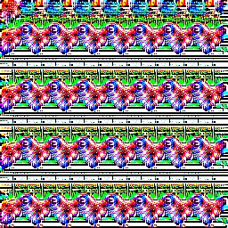
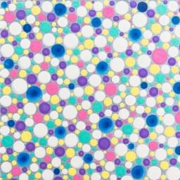
Image 1	Image 2
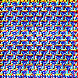
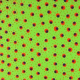
Image 3	Image 4
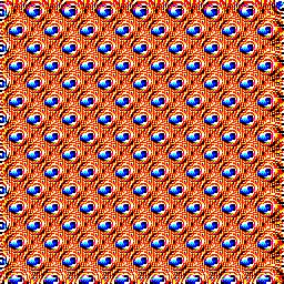
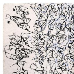
Image 5	Image 6
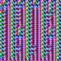
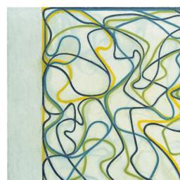
Image 7	Image 8
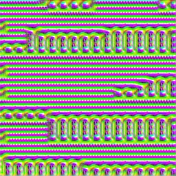
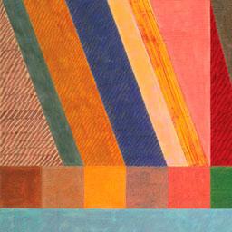
Image 9	Image 10

Figure 1: The Images used for Comparison

An online survey was given out, where 54 participants were asked to rate each image on a scale of 1-10, 10 being the most positive and 1 being the most negative. For each image the average rating and standard deviation are given in table 2. Notably, while the artificial images had much lower ratings, there was less variance in their ratings, suggesting the value of the ARTEMIS model is to produce images that humans will have a predictable reaction to.

Image	$\mu$	$\sigma$
Image 1	3.37	2.18
Image 2	5.03	2.63
Image 3	3.64	2.36
Image 4	3.94	2.32
Image 5	3.37	2.19
Image 6	6.26	2.16
Image 7	3.45	2.05
Image 8	6.59	2.53
Image 9	3.72	2.31
Image 10	6.93	2.25

Table 2: Caption

Conclusion

Contributions

This paper proposed a novel method of using generative adversarial networks with an ensemble of discriminators, each trained to classify images extracted from a different layer of the pretrained VGG-19 network. Trained on the WikiArt dataset, the network generated images that were akin to abstract art. Compared to manmade art, the artificially generated art was not as well received but there was less variability in how people reacted to the art.

Further Work

An obvious first step would be to use a new dataset. The WikiArt dataset contains almost no photographs, so it would be worthwhile to see how this model performs when trained using actual images. The WikiArt dataset is also extremely varied in the subjects it portrays and the scale and size involved, so a more homogenous dataset may be used for different results. Applying the multiple discriminator architecture to text would require a different pretrained style extractor than VGG-19, but would be promising.

Appendix A Architecture

Encoder

Though there were a few different input shapes, we made the encoder map them all to a standard noise size $\mathbb{R}^{2\times 2\times 64}$. The encoder was made of encoder blocks, parameterized by $c$, an integer representing the number of output channels in the encoder block, and $s$, the size of the stride:

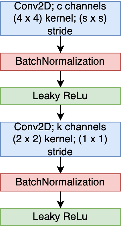
Figure 2: Encoder Block

First we wanted to make sure every layer had 64 channels. For input dim $\mathbb{R}^{256\times 256\times 3}$, we started with a convolutional block with 8 channels and kernel size $(8\times 8$ with stride $(1\times 1$, followed by BatchNormalization and Leaky ReLu. Then we had 3 encoder blocks, each with $s=1$, with $c=16,32,64$. For all the other input dimensions (see table 1), we held $s=1$ constant, and added layers where $c=\frac{1}{2}$ of the output channels of the last layer, until the output had 64 channels.

Then we wanted to shrink the spatial dimensions to be $(2\times 2)$. Holding $c$ constant, we used $s=2$, (this would halve the spatial dimensions each time), and applied encoder blocks until the output was $(2\times 2\times 64)$. We then added normal noise $\sim\mathcal{N}(0,1)$. Adding this noise will make the decoder more robust and lessen the chance of overfitting.

Decoder

The decoder mapped the noise to an image $\mathbb{R}^{2\times 2\times 64}\rightarrow\mathbb{R}^{256x256x3}$. It was mainly composed of batch decoder blocks shown in figure 3, parameterized by the boolean $attention\in\text{True}||\text{False}$, and $c$, the number of output channels.

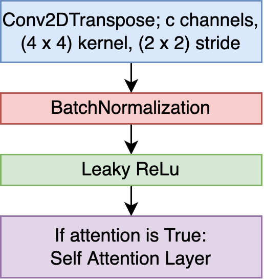
Figure 3: Batch Decoder Block

The decoder also contained group decoder blocks, show in figure 4, parameterized by $c$, the number of output channels, and $k$, the size of the kernel.

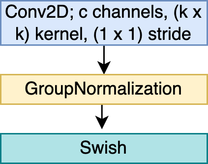
Figure 4: Group Decoder Block

The decoder consisted of 7 batch decoder blocks, where for each block, $c=\text{max}(32,c^{\prime})$, where $c^{\prime}$ was the amount of output channels in the prior batch decoder block, or the amount of channels in the input in the case of the first batch decoder block, and $attention$ was True for the first 4 blocks, and False for the last 3 batch decoder blocks. Following that, there were 3 group decoder blocks, with $c=(16,8,4$ and $k=(8,8,4)$, respectively. Finally, there was a Convolutional Layer with 3 output channels, a sigmoid activation function, and a rescaling layer to bound the values between 0 and 255, thus producing an image.

Discriminator

The discriminator(s) were composed of discriminator blocks shown in figure 5, parameterized by $c$, the number of output channels and $resnext$, a boolean of whether to use a ResNext layer Xie et al. (2016).

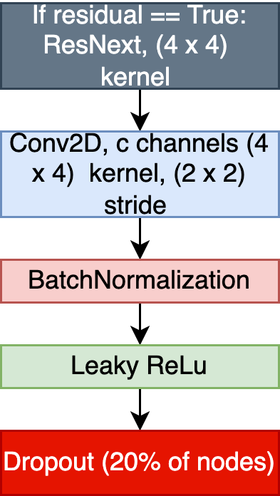
Figure 5: Discriminator Block

First, the discriminator had 4 discriminator blocks, each with $c=\frac{1}{2}c^{\prime}$, where $c^{\prime}$ was the amount of channels in the prior block, or the amount of channels in the input in the case of the first discriminator block, and for all but the first discriminator block, $resnext$ was True. After that, we flatten the input. Then we apply a fully-connected layer with 8 nodes, batch normalization, leaky ReLu, then the final dense layer with 1 node and sigmoid activation; this final node serves to output the (0,1) label.

References

- per (2017) Adversarial Perturbations of Deep Neural Networks, pages 311–342. 2017.
- Arjovsky et al. (2017) Martin Arjovsky, Soumith Chintala, and Léon Bottou. Wasserstein gan, 2017. URL https://arxiv.org/abs/1701.07875.
- Bahdanau et al. (2014) Dzmitry Bahdanau, Kyunghyun Cho, and Yoshua Bengio. Neural machine translation by jointly learning to align and translate, 2014. URL http://arxiv.org/abs/1409.0473. cite arxiv:1409.0473Comment: Accepted at ICLR 2015 as oral presentation.
- Caruana (1994) Rich Caruana. Learning many related tasks at the same time with backpropagation. In Proceedings of the 7th International Conference on Neural Information Processing Systems, NIPS’94, page 657–664, Cambridge, MA, USA, 1994. MIT Press.
- Dai et al. (2019) Tao Dai, Jianrui Cai, Yongbing Zhang, Shu-Tao Xia, and Lei Zhang. Second-order attention network for single image super-resolution. In 2019 IEEE/CVF Conference on Computer Vision and Pattern Recognition (CVPR), pages 11057–11066, 2019. doi: 10.1109/CVPR.2019.01132.
- Dong et al. (2020) Junyu Dong, Jun Liu, Kang Yao, Mike Chantler, Lin Qi, Hui Yu, and Muwei Jian. Survey of procedural methods for two-dimensional texture generation. Sensors, 20(4), 2020. ISSN 1424-8220. doi: 10.3390/s20041135. URL https://www.mdpi.com/1424-8220/20/4/1135.
- Elgammal et al. (2017) Ahmed M. Elgammal, Bingchen Liu, Mohamed Elhoseiny, and Marian Mazzone. CAN: creative adversarial networks, generating ”art” by learning about styles and deviating from style norms. CoRR, abs/1706.07068, 2017. URL http://arxiv.org/abs/1706.07068.
- Espejo-Garcia et al. (2020) Borja Espejo-Garcia, Nikos Mylonas, Loukas Athanasakos, Spyros Fountas, and Ioannis Vasilakoglou. Towards weeds identification assistance through transfer learning. Computers and Electronics in Agriculture, 171:105306, 2020. ISSN 0168-1699. doi: https://doi.org/10.1016/j.compag.2020.105306. URL https://www.sciencedirect.com/science/article/pii/S0168169919319854.
- Gatys et al. (2015) Leon A. Gatys, Alexander S. Ecker, and Matthias Bethge. A neural algorithm of artistic style. CoRR, abs/1508.06576, 2015. URL http://arxiv.org/abs/1508.06576.
- Gooch et al. (2004) Bruce Gooch, Erik Reinhard, and Amy Gooch. Human facial illustrations: Creation and psychophysical evaluation. ACM Trans. Graph., 23(1):27–44, jan 2004. ISSN 0730-0301. doi: 10.1145/966131.966133. URL https://doi.org/10.1145/966131.966133.
- Goodfellow et al. (2014) Ian J. Goodfellow, Jean Pouget-Abadie, Mehdi Mirza, Bing Xu, David Warde-Farley, Sherjil Ozair, Aaron Courville, and Yoshua Bengio. Generative adversarial networks, 2014.
- Gregor et al. (2015) Karol Gregor, Ivo Danihelka, Alex Graves, and Daan Wierstra. DRAW: A recurrent neural network for image generation. CoRR, abs/1502.04623, 2015. URL http://arxiv.org/abs/1502.04623.
- Guan et al. (2018) Qingji Guan, Yaping Huang, Zhun Zhong, Zhedong Zheng, Liang Zheng, and Yi Yang. Diagnose like a radiologist: Attention guided convolutional neural network for thorax disease classification. CoRR, abs/1801.09927, 2018. URL http://arxiv.org/abs/1801.09927.
- Gulrajani et al. (2017) Ishaan Gulrajani, Faruk Ahmed, Martín Arjovsky, Vincent Dumoulin, and Aaron C. Courville. Improved training of wasserstein gans. CoRR, abs/1704.00028, 2017. URL http://arxiv.org/abs/1704.00028.
- Gutierrez et al. (2020) Jorge Gutierrez, Julien Rabin, Bruno Galerne, and Thomas Hurtut. On demand solid texture synthesis using deep 3d networks. CoRR, abs/2001.04528, 2020. URL https://arxiv.org/abs/2001.04528.
- Ham et al. (2020) Hyungrok Ham, Tae Joon Jun, and Daeyoung Kim. Unbalanced gans: Pre-training the generator of generative adversarial network using variational autoencoder. CoRR, abs/2002.02112, 2020. URL https://arxiv.org/abs/2002.02112.
- Hertzmann (1998) Aaron Hertzmann. Painterly rendering with curved brush strokes of multiple sizes. In Proceedings of the 25th Annual Conference on Computer Graphics and Interactive Techniques, SIGGRAPH ’98, page 453–460, New York, NY, USA, 1998. Association for Computing Machinery. ISBN 0897919998. doi: 10.1145/280814.280951. URL https://doi.org/10.1145/280814.280951.
- Ioffe and Szegedy (2015) Sergey Ioffe and Christian Szegedy. Batch normalization: Accelerating deep network training by reducing internal covariate shift. CoRR, abs/1502.03167, 2015. URL http://arxiv.org/abs/1502.03167.
- Jignesh Chowdary et al. (2020) G. Jignesh Chowdary, Narinder Singh Punn, Sanjay Kumar Sonbhadra, and Sonali Agarwal. Face mask detection using transfer learning of inceptionv3. In Ladjel Bellatreche, Vikram Goyal, Hamido Fujita, Anirban Mondal, and P. Krishna Reddy, editors, Big Data Analytics. Springer International Publishing, 2020. ISBN 978-3-030-66665-1.
- Johnson et al. (2016) Justin Johnson, Alexandre Alahi, and Li Fei-Fei. Perceptual losses for real-time style transfer and super-resolution. CoRR, abs/1603.08155, 2016. URL http://arxiv.org/abs/1603.08155.
- Kolokolova et al. (2020) Antonina Kolokolova, Mitchell Billard, Robert Bishop, Moustafa Elsisy, Zachary Northcott, Laura Graves, Vineel Nagisetty, and Heather Patey. Gans & reels: Creating irish music using a generative adversarial network. CoRR, abs/2010.15772, 2020. URL https://arxiv.org/abs/2010.15772.
- Li and Wand (2016) Chuan Li and Michael Wand. Combining markov random fields and convolutional neural networks for image synthesis. CoRR, abs/1601.04589, 2016. URL http://arxiv.org/abs/1601.04589.
- Li et al. (2017) Yijun Li, Chen Fang, Jimei Yang, Zhaowen Wang, Xin Lu, and Ming-Hsuan Yang. Diversified texture synthesis with feed-forward networks. 2017 IEEE Conference on Computer Vision and Pattern Recognition (CVPR), pages 266–274, 2017.
- Liu et al. (2018) Hanwen Liu, Pablo Navarrete Michelini, and Dan Zhu. Artsy-gan: A style transfer system with improved quality, diversity and performance. In 2018 24th International Conference on Pattern Recognition (ICPR), pages 79–84, 2018. doi: 10.1109/ICPR.2018.8546172.
- Luan et al. (2017) Fujun Luan, Sylvain Paris, Eli Shechtman, and Kavita Bala. Deep photo style transfer. CoRR, abs/1703.07511, 2017. URL http://arxiv.org/abs/1703.07511.
- Luong et al. (2015) Minh-Thang Luong, Hieu Pham, and Christopher D. Manning. Effective approaches to attention-based neural machine translation. CoRR, abs/1508.04025, 2015. URL http://arxiv.org/abs/1508.04025.
- Misra (2019) Diganta Misra. Mish: A self regularized non-monotonic neural activation function. CoRR, abs/1908.08681, 2019. URL http://arxiv.org/abs/1908.08681.
- Mnih et al. (2014) Volodymyr Mnih, Nicolas Heess, Alex Graves, and Koray Kavukcuoglu. Recurrent models of visual attention. CoRR, abs/1406.6247, 2014. URL http://arxiv.org/abs/1406.6247.
- Nagpal et al. (2020) Sidhant Nagpal, Siddharth Verma, Shikhar Gupta, and Swati Aggarwal. A guided learning approach for generative adversarial networks. 2020 International Joint Conference on Neural Networks (IJCNN), pages 1–8, 2020.
- Park and Lee (2019) Dae Young Park and Kwang Hee Lee. Arbitrary style transfer with style-attentional networks. 2019 IEEE/CVF Conference on Computer Vision and Pattern Recognition (CVPR), pages 5873–5881, 2019.
- Raad et al. (2017) Lara Raad, Axel Davy, Agnès Desolneux, and Jean-Michel Morel. A survey of exemplar-based texture synthesis. CoRR, abs/1707.07184, 2017. URL http://arxiv.org/abs/1707.07184.
- Radford et al. (2015) Alec Radford, Luke Metz, and Soumith Chintala. Unsupervised representation learning with deep convolutional generative adversarial networks, 2015. URL http://arxiv.org/abs/1511.06434. cite arxiv:1511.06434Comment: Under review as a conference paper at ICLR 2016.
- Ramachandran et al. (2017) Prajit Ramachandran, Barret Zoph, and Quoc V. Le. Searching for activation functions. CoRR, abs/1710.05941, 2017. URL http://arxiv.org/abs/1710.05941.
- Saeed et al. (2019) Asir Saeed, Suzana Ilic, and Eva Zangerle. Creative gans for generating poems, lyrics, and metaphors. CoRR, abs/1909.09534, 2019. URL http://arxiv.org/abs/1909.09534.
- Saleh and Elgammal (2015) Babak Saleh and Ahmed M. Elgammal. Large-scale classification of fine-art paintings: Learning the right metric on the right feature. CoRR, abs/1505.00855, 2015. URL http://arxiv.org/abs/1505.00855.
- Salimans et al. (2016) Tim Salimans, Ian J. Goodfellow, Wojciech Zaremba, Vicki Cheung, Alec Radford, and Xi Chen. Improved techniques for training gans. CoRR, abs/1606.03498, 2016. URL http://arxiv.org/abs/1606.03498.
- Santurkar et al. (2019) Shibani Santurkar, Dimitris Tsipras, Andrew Ilyas, and Aleksander Madry. How does batch normalization help optimization?, 2019.
- Simonyan and Zisserman (2015) Karen Simonyan and Andrew Zisserman. Very deep convolutional networks for large-scale image recognition. In International Conference on Learning Representations, 2015.
- Tan et al. (2018) Chuanqi Tan, Fuchun Sun, Tao Kong, Wenchang Zhang, Chao Yang, and Chunfang Liu. A survey on deep transfer learning. CoRR, abs/1808.01974, 2018. URL http://arxiv.org/abs/1808.01974.
- Ulyanov et al. (2016) Dmitry Ulyanov, Vadim Lebedev, Andrea Vedaldi, and Victor S. Lempitsky. Texture networks: Feed-forward synthesis of textures and stylized images. CoRR, abs/1603.03417, 2016. URL http://arxiv.org/abs/1603.03417.
- Vaswani et al. (2017) Ashish Vaswani, Noam Shazeer, Niki Parmar, Jakob Uszkoreit, Llion Jones, Aidan N. Gomez, Lukasz Kaiser, and Illia Polosukhin. Attention is all you need. CoRR, abs/1706.03762, 2017. URL http://arxiv.org/abs/1706.03762.
- Wang et al. (2021) Pei Wang, Yijun Li, and Nuno Vasconcelos. Rethinking and improving the robustness of image style transfer. CoRR, abs/2104.05623, 2021. URL https://arxiv.org/abs/2104.05623.
- Wang et al. (2017) Xiaolong Wang, Ross B. Girshick, Abhinav Gupta, and Kaiming He. Non-local neural networks. CoRR, abs/1711.07971, 2017. URL http://arxiv.org/abs/1711.07971.
- Wang et al. (2018) Xintao Wang, Ke Yu, Shixiang Wu, Jinjin Gu, Yihao Liu, Chao Dong, Chen Change Loy, Yu Qiao, and Xiaoou Tang. ESRGAN: enhanced super-resolution generative adversarial networks. CoRR, abs/1809.00219, 2018. URL http://arxiv.org/abs/1809.00219.
- Wen et al. (2019) Long Wen, X. Y. Li, Xinyu Li, and Liang Gao. A new transfer learning based on vgg-19 network for fault diagnosis. 2019 IEEE 23rd International Conference on Computer Supported Cooperative Work in Design (CSCWD), pages 205–209, 2019.
- Wikipedia (2022) Wikipedia. Texture (visual arts) –Wikipedia, the free encyclopedia. https://en.wikipedia.org/wiki/Texture_(visual_arts), 2022. [Online; accessed 16-February-2022].
- Wilmot et al. (2017) Pierre Wilmot, Eric Risser, and Connelly Barnes. Stable and controllable neural texture synthesis and style transfer using histogram losses. CoRR, abs/1701.08893, 2017. URL http://arxiv.org/abs/1701.08893.
- Wu et al. (2018) Jiajun Wu, Chengkai Zhang, Xiuming Zhang, Zhoutong Zhang, William T. Freeman, and Joshua B. Tenenbaum. Learning shape priors for single-view 3d completion and reconstruction. CoRR, abs/1809.05068, 2018. URL http://arxiv.org/abs/1809.05068.
- Xian et al. (2017) Wenqi Xian, Patsorn Sangkloy, Jingwan Lu, Chen Fang, Fisher Yu, and James Hays. Texturegan: Controlling deep image synthesis with texture patches. CoRR, abs/1706.02823, 2017. URL http://arxiv.org/abs/1706.02823.
- Xie et al. (2016) Saining Xie, Ross B. Girshick, Piotr Dollár, Zhuowen Tu, and Kaiming He. Aggregated residual transformations for deep neural networks. CoRR, abs/1611.05431, 2016. URL http://arxiv.org/abs/1611.05431.
- Xu et al. (2021) Wenju Xu, Chengjiang Long, Ruisheng Wang, and Guanghui Wang. DRB-GAN: A dynamic resblock generative adversarial network for artistic style transfer. CoRR, abs/2108.07379, 2021. URL https://arxiv.org/abs/2108.07379.
- Zhang et al. (2019) Han Zhang, Ian Goodfellow, Dimitris Metaxas, and Augustus Odena. Self-attention generative adversarial networks. In Kamalika Chaudhuri and Ruslan Salakhutdinov, editors, Proceedings of the 36th International Conference on Machine Learning, volume 97 of Proceedings of Machine Learning Research, pages 7354–7363. PMLR, 09–15 Jun 2019. URL https://proceedings.mlr.press/v97/zhang19d.html.
- Zhang et al. (2018) Yulun Zhang, Kunpeng Li, Kai Li, Lichen Wang, Bineng Zhong, and Yun Fu. Image super-resolution using very deep residual channel attention networks. CoRR, abs/1807.02758, 2018. URL http://arxiv.org/abs/1807.02758.
- Zhu et al. (2017) Jun-Yan Zhu, Taesung Park, Phillip Isola, and Alexei A. Efros. Unpaired image-to-image translation using cycle-consistent adversarial networks. CoRR, abs/1703.10593, 2017. URL http://arxiv.org/abs/1703.10593.