A cool, magnetic white dwarf accreting planetary debris

Abstract

We present an analysis of spectroscopic data of the cool, highly magnetic and polluted white dwarf 2MASS J0916$-$4215. The atmosphere of the white dwarf is dominated by hydrogen, but numerous spectral lines of magnesium, calcium, titanium, chromium, iron, strontium, along with Li i, Na i, Al i, and K i lines, are found in the incomplete Paschen-Back regime, most visibly, in the case of Ca ii lines. Extensive new calculations of the Paschen-Back effect in several spectral lines are presented and results of the calculations are tabulated for the Ca ii H&K doublet. The abundance pattern shows a large lithium and strontium excess, which may be viewed as a signature of planetary debris akin to Earth’s continental crust accreted onto the star, although the scarcity of silicon indicates possible dilution in bulk Earth material. Accurate abundance measurements proved sensitive to the value of the broadening parameter due to collisions with neutral hydrogen ($\Gamma_{\rm\text{H\,{i}}}$), particularly in saturated lines such as the resonance lines of Ca i and Ca ii. We found that $\Gamma_{\rm\text{H\,{i}}}$ if formulated with values from the literature could be overestimated by a factor of 10 in most resonance lines.

1 Introduction

The spectroscopic analysis of magnetic white dwarfs covers a wide range of field strengths from $10^{-3}$ to $10^{3}$ MG. The hydrogen and helium line spectra have been extensively modelled over the whole range of field strength (Garstang & Kemic, 1974; Schimeczek & Wunner, 2014) but difficulties remain in modelling the field geometry. With few exceptions, magnetic white dwarf are assumed to harbor offset dipole fields. The study of trace elements, from lithium to iron and beyond, in magnetic white dwarf spectra is in its infancy.

Recent studies have tackled the problem of line formation in the full Paschen-Back regime in high magnetic fields (Zhao, 2018; Hollands et al., 2023), while Kemic (1975) initiated the first study of the Ca ii H&K doublet in the incomplete Paschen-Back regime (see also Hardy, Dufour, & Jordan, 2017), i.e., between the anomalous regime and the full Paschen-Back regime where the lines assume the shape of a simple polarization triplet ($\pi$ and $\sigma_{\pm}$) with energy separations simply proportional to the magnetic field strength.

Meaningful results with abundances of various elements from sodium to iron were obtained at relatively low field in the anomalous Zeeman regime (Kawka & Vennes, 2011, 2014; Kawka et al., 2019). In their study of low-field DZ white dwarfs Hollands et al. (2021) encountered the line spectrum of potassium in the incomplete Paschen-Back regime and the lithium spectrum in the full regime. The behavior of spectral lines in magnetic white dwarfs is not yet fully understood and new calculations in fields ranging from 1 to 100 MG are clearly warranted.

Heavy element pollution in white dwarf atmospheres is well documented. Restricting the discussion to cool white dwarfs, accretion of external material, irrespective of the source, is the essential mechanism (Dupuis, Fontaine, & Wesemael, 1993). In hot white dwarfs, where selective radiation pressure plays an important role (Chayer et al., 1995), the composition of the atmosphere is dictated by local physical conditions. However, in cool convective white dwarfs the composition of the atmosphere offers clues to the nature and composition of the source itself. Debris material from disrupted planetary bodies is the most likely source (Zuckerman et al., 2007; Jura & Young, 2014; Zuckerman & Young, 2018; Veras, 2021) but variations over this theme rely heavily on the accuracy of abundance measurements.

Based on a large sample of cool, polluted white dwarfs Hollands, Gänsicke, & Koester (2018) observed a range of likely sources, from (Earth’s) crust-like to core-like based on key abundance proportions: calcium, iron or magnesium divided by a weighted sum of the three, which typify, respectively, the Earth’s crust, core, and mantle. Interestingly, most objects point towards a mixture of sources which is labelled bulk Earth. Further, studies of oxygen-polluted white dwarfs have demonstrated evidence of the stoichiometric balance of elements in rock-forming oxides in the accreted material, bearing a close resemblance to rocky bodies in the solar system (Klein et al., 2010; Xu et al., 2014; Doyle et al., 2023). The detection of the light elements, beryllium and lithium, has raised the possibility that such polluted white dwarfs might be used as tracers of spallation environments (Klein et al., 2021; Doyle, Desch, & Young, 2021), differentiation into planetary-crust material (Hollands et al., 2021), and/or windows into the early universe and Big Bang Nucleosynthesis (Kaiser et al., 2021). Overall, the study of abundance patterns in white dwarf stars reveals a complicated history of past and present interaction with their circumstellar environment.

In this context, we present new echelle spectra of the magnetic white dwarf 2MASS J0916$-$4215 (Section 2) revealing several spectral lines formed in the incomplete Paschen-Back regime in a 11-12 MG magnetic field (Section 3). 2MASS J0916$-$4215 is a new cool, magnetic white dwarf with trace elements in a hydrogen-rich atmosphere. The abundance pattern shows a two orders of magnitude excess in lithium and an overall distribution, with the notable exception of silicon, pointing out to a primordial origin for the material analogous to Earth’s continental crust. A discussion and summary are presented in Section 4. We describe in Appendix A our new calculations of the Paschen-Back effect for all spectral lines found in 2MASS J0916$-$4215.

2 Observations

The star 2MASS J0916$-$4215 appears as a white dwarf candidate in the catalogue of Gentile Fusillo et al. (2019). We first observed 2MASS J0916$-$4215 with the MIKE double echelle spectrograph attached to the Magellan 2 - Clay telescope at Las Campanas Observatory on UT 2021 December 18 and 19. We set the slit width to 1 arcsec to provide a resolution $R=\lambda/\Delta\lambda=22\,000$ and 28 000 on the red and blue sides, respectively (Bernstein et al., 2003). We obtained an additional spectrum with the MagE (Magellan echellette) spectrograph (Marshall et al., 2008) attached to the Magellan 1 - Baade telescope on UT 2022 March 23. We set the slit width to 0.5 arcsec to provide a resolution $R=8000$. The spectra were corrected for telluric absorption using a template provided by the TAPAS database (Bertaux et al., 2014) and using the telluric routine within the Image Reduction and Analysis Facility (IRAF). We employ air wavelengths throughout this work.

We collected optical and infrared photometric measurements from the SkyMapper survey (Onken et al., 2019), Two Micron All Sky Survey (2MASS: Skrutskie et al., 2006) and Wide-field Infrared Survey Explorer (WISE: Cutri et al., 2013; Marocco et al., 2021). These are listed in Table 1 together with photometric and astrometric data from the Gaia Data Release 3 (Gaia Collaboration et al., 2022). 2MASS J0916$-$4215 is a nearby white dwarf well within the 40 pc sample (Gentile Fusillo et al., 2019; O’Brien et al., 2023), also known as WD J091600.94$-$421520.68 (WD J0916$-$4215) or Gaia DR3 5427528254746168192, and was tentatively classified as a magnetic white dwarf (O’Brien et al., 2023).

2MASS J0916$-$4215 was observed with the Transiting Exoplanet Survey Satellite (TESS: Ricker et al., 2015) in sectors 35, 36 and 62. The TESS bandpass has a spectral range from 6000 to 10 000Å. Sector 35 was observed from 2021 February 9 to March 6, sector 36 was observed from 2021 March 7 to April 1 and sector 62 was observed from 2023 February 12 to March 10.

Table 1: Astrometry and photometry of 2MASS J0916$-$4215.

Parameter		Measurement			Ref.
RA (J2000)		09h16m00$\aas@@fstack{s}$94			1
Dec (J2000)		-42°15′20$\aas@@fstack{\prime\prime}$68			1
$\mu_{\alpha}\cos{\delta}$ (mas yr-1)		$-24.67\pm 0.04$			1
$\mu_{\delta}$ (mas yr-1)		$-203.56\pm 0.05$			1
$\pi$ (mas)		$44.35\pm 0.04$			1
Photometry
Band	Measurement	Ref.	Band	Measurement	Ref.
$G$	$16.566\pm 0.003$	1	$J$	$15.307\pm 0.064$	3
$G_{BP}$	$17.003\pm 0.010$	1	$H$	$15.260\pm 0.101$	3
$G_{RP}$	$15.961\pm 0.025$	1	$K$	$14.890\pm 0.124$	3
$g$	$17.039\pm 0.050$	2	$W1$	$14.770\pm 0.015$	4
$r$	$16.666\pm 0.036$	2	$W2$	$14.725\pm 0.020$	4
$i$	$16.311\pm 0.017$	2	$W3$	$<12.363$	5
$z$	$16.283\pm 0.020$	2

References: (1) Gaia Collaboration et al. (2022); (2) Onken et al. (2019); (3) Skrutskie et al. (2006); (4) Marocco et al. (2021); (5) Cutri et al. (2013).

3 Analysis

The high-dispersion spectra show heavy element lines in a cool hydrogen-rich atmosphere. Nominally, the spectrum is classified as DZAH owing to the presence of strong, magnetic-displaced magnesium, calcium and iron lines and a much weaker hydrogen line. The presence of a weak, Zeeman-split H$\alpha$ line could imply a temperature slightly above 5 000 K in a hydrogen-dominated atmosphere but it could also imply a higher temperature, e.g., $\approx 8\,000$ K, in a helium-dominated atmosphere. The temperature and gravity may be constrained further with an analysis of the spectral energy distribution (Section 3.1). All spectral lines display a pattern revealing the presence of a surface average magnetic field of approximately 11.3 MG in strength. With other closely related polluted, hydrogen-rich, magnetic white dwarfs (Kawka et al., 2019) that were classified as DAZH white dwarfs, 2MASS J0916$-$4215 is part of a class of objects accreting material from their circumstellar environment.

Many spectral lines in 2MASS J0916$-$4215 follow an apparent triplet pattern which at this field strength implies the onset of the full Paschen-Back regime. Closer examination reveals a more complex pattern, particularly in the case of the Ca ii H&K doublet. The $\pi$ and $\sigma_{\pm}$ components follow a pattern already described by Kemic (1975) which transitions between the low-field anomalous Zeeman and the high-field full Paschen-Back triplet pattern with dominant components shifted by $\Delta E=0$ and $\pm\mu_{0}B$ and vanishing components at $\pm 2\mu_{0}B$, where $\mu_{0}=e\hbar/(2m_{e}c)$ is the Bohr magneton and $B$ is the magnetic field strength (see Appendix A). In addition, each polarization component is itself a doublet.

This pattern, which can be described as belonging to the incomplete Paschen-Back regime (Landi Degl’Innocenti & Landolfi, 2004), shows split $\pi$ and $\sigma$ components leaving six strong line components that are characteristic of ²S - ²P^o spectral lines (Fig. 1). For example, sitting close to the $\pi$ components of the Ca ii H&K line, split $\pi$ components of the Al i $\lambda$3955 line are evident. In the Paschen-Back regime the individual polarization components develop a doublet appearance for fine-structure doublets, e.g., Ca ii H&K or Al i $\lambda$3955, or a triplet appearance for fine-structure triplets, e.g., Mg i $\lambda$5178.  This pattern deviates strongly from the anomalous Zeeman pattern explored by Kawka et al. (2019) in the lower field ($\lesssim 0.3$ MG) DAZH white dwarf NLTT 7547. The Ca ii and Al i lines in a field of $\approx$11.3 MG belong to the incomplete Paschen-Back regime.

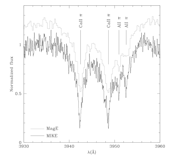
Figure 1: MIKE (black line) and MagE (grey line) echelle spectra showing both Ca ii $\lambda$3945 and Al i $\lambda 3955$ split $\pi$ components in the incomplete Paschen-Back regime. Wavelengths in all figures are in air.

3.1 Model atmospheres and stellar parameters

We computed a series of convective model atmospheres containing trace abundance of heavy elements. The electron density is computed self-consistently with the ionization equilibrium of all constituents of the atmosphere including most associated metal monohydrides (Sauval & Tatum, 1984).

We note that Bédard, Bergeron, & Fontaine (2017) found that convective energy transfer may be suppressed in a $\approx$10 000 K hydrogen-rich white dwarf following their spectroscopic analysis of the low-field magnetic white dwarf WD 2105$-$820. Indeed, Tremblay et al. (2015) predicted that even a weak field ($\approx 5$ kG) would partially suppress convective energy transfer in the line forming region of an $\approx$10 000 K hydrogen-rich white dwarf, although vertical mixing may still take place (see also Cunningham et al., 2021). Similar 3D radiation magnetohydrodynamic calculations applicable to cooler, predominantly neutral atmosphere of cool ($\approx 5\,000$ K) DAZ white dwarfs (Kawka et al., 2019) are not currently available, but setting the plasma-$\beta$ parameter to unity in the line-forming region allows to estimate a critical field of the order of $\approx 40$ kG (Cunningham et al., 2021). Although mixing may not be suppressed, the maximum extent of the mixing region under the influence of a strong magnetic field is uncertain but it will be assumed identical to that of a non-magnetic hydrogen envelope (see Section 3.4). As indicated above, we adopted convective model atmosphere structures.

We first estimated the temperature and surface gravity using all available photometric measurements and the Gaia parallax (Table 1). Figure 2 shows a model atmosphere analysis of these measurements: 2MASS J0916$-$4215 is a cool white dwarf with $T_{\rm eff}=5\,250\pm 250$ K, and $\log{g}=8.13\pm 0.13$, where the surface gravity $g$ is expressed in cm s^-2. A weak H$\alpha$ line confirms its low temperature and its hydrogen-rich composition. The strength of the H$\alpha$ $\pi$ component restricts further the range of acceptable parameters with error bars $\sigma(T_{\rm eff})=100$ K and $\sigma(\log{g})=0.06$. We conclude that

$$T_{\rm eff}=5\,250\pm 100\,{\rm K},\ {\rm and}\ \log{g}=8.13\pm 0.06$$

Using Gaia data, Gentile Fusillo et al. (2019) estimated a temperature $T_{\rm eff}=5056$ and 5142 K and a surface gravity of $\log{g}=$7.99 and 8.05, based on pure-helium and pure-hydrogen models, respectively, in agreement with our own measurements. The stellar parameters correspond to a white dwarf mass of $0.66\pm 0.04~{}M_{\odot}$ and cooling age of $4.8\pm 0.8$ Gyr. We used the evolutionary mass-radius relations of Benvenuto & Althaus (1999). Note that a slightly longer cooling age of 6 Gyr is obtained with calculations generated by the Montréal White Dwarf Database (MWDD, Bédard et al., 2020) .

2MASS J0916$-$4215 belongs to a class of polluted, cool magnetic white dwarfs originally identified in a high proper-motion surveys such as G 77-50 (Farihi et al., 2011), NLTT 10480 (Kawka & Vennes, 2011), NLTT 43806 (Zuckerman et al., 2011), and NLTT 7547 (Kawka et al., 2019). 2MASS J0916$-$4215 extends the distribution towards higher fields which now covers average surface fields from 70 kG to 11.3 MG.

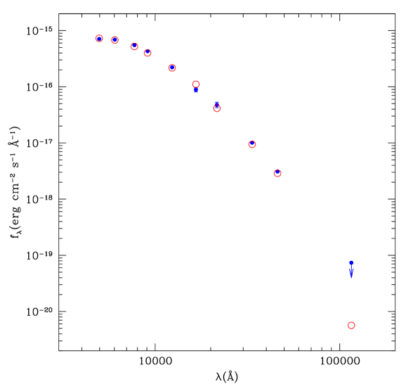
Figure 2: Spectral energy distribution of the cool white dwarf 2MASS J0916$-$4215 (blue squares) and best fit synthetic colors (open red circles). The photometric data points are listed in Table 1. We include the Wise W3 band at 12 $\mu$ as an upper limit.

3.2 Field strength and structure, and the Paschen-Back effect

The wavelength extent of the triplet line pattern in some lines, e.g., Mg i $\lambda 5178$, is given by

$$\Delta\lambda(\text{\AA})=4.67\times 10^{-7}\lambda^{2}(\text{\AA})B({\rm MG})$$ (1)

and corresponds to an average surface field of $\approx$11.3 MG. Despite large wavelength shifts most lines appear narrow. The $\pi$ components are relatively stable in the Paschen-Back regime resulting in minimal broadening when integrating over a dipole field distribution. However the appearance of the $\sigma$ components is sensitive to the field distribution and the offset dipole is a common feature in modelling magnetic white dwarf spectra as it tends to homogenize the field and narrow the spectral lines as observed in 2MASS J0916$-$4215. We computed the field geometry following Martin & Wickramasinghe (1981), Martin & Wickramasinghe (1984), and Achilleos & Wickramasinghe (1989). An approximate relationship between the dipole field strength $B_{\rm d}$ and its surface average $B_{\rm S}$ is given by

$$B_{\rm S}\approx 0.7(1+a_{z})B_{\rm d}$$ (2)

where $a_{z}$ is the offset along the $z$ axis expressed as a fraction of the stellar radius. A centered dipole is located at $a_{z}=0$. Adopting $a_{z}=-0.3$ would approximately correspond to an offset dipole field strength of 22 MG close to our dipole field model. The line positions and shapes in the MagE and MIKE spectra are matched with models at $B_{\rm d}=24$ MG and $a_{z}=-0.3$ inclined at $i=70^{\circ}$. Other examples of offset dipole modelling are presented by Vennes et al. (2018).

Other than for the Ca ii H&K doublet (Kemic, 1975) Paschen-Back calculations are not available in the range of magnetic field reached in 2MASS J0916$-$4215. The Landi Degl’Innocenti & Landolfi (2004) theory includes only the linear Zeeman effect and generally applies to low-field stars. In higher field objects such as this one, quadratic field effects as discussed by Kemic (1975) in the case of the Ca ii H&K doublet remain to be explored. As noted earlier by Kawka et al. (2019), both sets of calculations, Kemic (1975) and Landi Degl’Innocenti & Landolfi (2004), are in agreement at lower fields ($<<$10 MG) where quadratic effects are negligible, although Kawka et al. (2019) incorrectly stated that Landi Degl’Innocenti & Landolfi (2004) included the effect of quadratic terms. For a general application to spectral lines observed in 2MASS J0916$-$4215 it was therefore necessary to develop further the theory elaborated by Landi Degl’Innocenti & Landolfi (2004) and include the quadratic terms when computing atomic energy levels embedded in an external magnetic field (Appendix A).

Figure 3 shows a series of Ca ii H&K synthetic spectra illustrating the Paschen-Back effect with increasing dipole field strength for a model appropriate for the white dwarf 2MASS J0916$-$4215 (see Section 3.3). The pattern greatly varies with field strength and a model with a dipole field of 20 MG closely resembles the observed calcium spectrum (Fig. 1).

Figure 3: Morphology of the Ca ii H&K doublet with increasing dipole field strength ($B_{\rm d}$) from 0 to 40 MG (from bottom to top). The field geometry (inclination and offset) and stellar parameters ($T_{\rm eff}=5\,250$K and $\log{g}=8.13$) of the models are appropriate for the subject of this study, 2MASS J0916$-$4215. The transition from the anomalous Zeeman regime (depicted at 2 MG) to the full Paschen-Back regime (depicted at 40 MG) sees the number of visible line components drop from 10 to 6, with the resulting pattern falling in three groups, the central $\pi$ components and the $\sigma_{\pm}$ components resembling a simple Zeeman triplet. The spectra are shifted vertically by one unit for clarity.

Figure 4 shows predicted line positions as a function of magnetic field strength for the singlet Li i $\lambda$6707 and the triplet Ca i $\lambda$6142. Adopting a field of 11.3 MG corresponding to the average surface field in 2MASS J0916$-$4215, we find a quadratic shift of $\Delta\varv=-672.4$ km s^-1 in the $\pi$ component of $\lambda$6142 while it retains a triplet structure, but this shift is only $\Delta\varv=10.4$ km s^-1 in the $\pi$ component of $\lambda$6707. Our stellar radial velocity measurement for 2MASS J0916$-$4215 is based on a set of these narrow $\pi$ line components. All lines are affected with varying degrees by linear and quadratic shifts. We initially selected Li i $\lambda$6707 as the primary velocity indicator because of its small predicted velocity shift. This single line sets the observed heliocentric radial velocity at $\varv_{r}=21.3$ km s^-1. The gravitational redshift correction will be considered in Section 3.5. Next, we selected 8 additional lines with increasing Paschen-Back shifts ($\Delta\varv$ in km s^-1) in order to evaluate the reliability of our Paschen-Back models in predicting line shifts: Ca ii$\lambda$3945 ($\Delta\varv=5.8$), K i $\lambda$7676 ($\Delta\varv=-33.1$), Na i $\lambda$5891 ($\Delta\varv=-33.7$), Ca i $\lambda 4226$ ($\Delta\varv=-35.3$), Sr i $\lambda$4607 ($\Delta\varv=-44.0$), Al i $\lambda$3955 ($\Delta\varv=-281.5$), Mg i $\lambda$5178 ($\Delta\varv=-425.0$), Ca i $\lambda$6142 ($\Delta\varv=-672.4$). The average and dispersion of the radial velocity measurements are $\varv=20.2\pm 8$ and excluding two outliers ($\lambda$ 6142 and $\lambda$5178) we find $\Delta\varv=20.6\pm 3.7$ km s^-1. We conclude, based on 7 good lines, that $\varv_{r}=21\pm 4$ km s^-1. Figure 4 compares the Paschen-Back calculations to the observed line positions. The predicted $\lambda$6142 line position is in error by $-13$ km s^-1, or $\approx$2% of the total shift relative to the observed line position (assuming $\varv_{r}=21$ km s^-1), while the predicted position of the $\lambda$6707 line is in error by $\approx$0.7 km s^-1, or $\approx$7%. Inclusion of the quadratic shift is not only essential for radial velocity measurements but also in securing correct line identifications.

Figure 4: Linear (short dashed lines) and the sum of linear and quadratic (full lines) Paschen-Back calculations compared to observed line positions in the stellar rest frame (open squares, see text). Assuming an average surface field of 11.3 MG, the Ca i$~{}\lambda$6142 line is shifted by $\approx-$14Å by the quadratic effect in agreement with the observed line positions, while the Li i $\lambda$6707 is shifted by only +0.2Å. The mean zero-field wavelength of the Ca i multiplet is shown with a long dashed line.

3.3 Line profile and spectral analysis

The opacity of individual line components is calculated using normalized Lorentzian profiles,

$$\Phi_{\nu}=\frac{1}{\pi}\frac{\Gamma/4\pi}{(\nu-\nu_{c})^{2}+(\Gamma/4\pi)^{2}}$$ (3)

convoluted with Doppler profiles. Here, $\nu_{c}$ is the frequency of the shifted line centre, and $\Gamma$ is the sum of the natural width and the broadening parameter, i.e, the full-width at half-maximum expressed in rad s^-1. In cool hydrogen-rich atmosphere, line broadening is dominated by collisions with neutral hydrogen atoms (Barklem, Piskunov, & O’Mara, 2000b).

The hydrogen lines were modelled following the quadratic Zeeman calculations of Schimeczek & Wunner (2014) and using self-broadening parameters of Barklem, Piskunov, & O’Mara (2000a). We included the linear and quadratic energy corrections in the calculation of the Boltzmann factors for all energy levels.

The spectra show numerous Ca i excited lines along with the resonance line Ca i $\lambda$4226. The excited lines emerge between 1.9 and 2.5 eV above the ground-state and should only be weakly populated at temperatures near 5 250 K as the Boltzmann factor for the excited states ranges between $3\times 10^{-3}$ and $10^{-2}$ relative to the ground-state.

Table 2: Calcium broadening parameters at full-width half-maximum $\Gamma/n_{\rm\text{H\,{i}}}$ (rad s^-1cm³), $T=5\,250$ K, and population departures.

	(1)	(2)		(3)	(4)		(5)	(6)
Ion	$\lambda_{ik}$	$\log{({\Gamma}/{n_{\rm\text{H\,{i}}}})}^{a}$		$\log{({\Gamma}/{n_{\rm\text{H\,{i}}}})}^{b}$	$\log{\rm Ca/H}$		$\Delta\log{\Gamma}$	$\log{\rm Ca/H}$
	(Å)				($+$8.0)			($+$6.7)
Ca i	4226	$-$7.88		$-$7.67	$+$0.5		$-$1.0	$+$0.0
	4445	$-$7.53		$-$7.26	$+$1.5		$-$0.0	$+$0.0
	5266	$-$7.89		$-$7.62	$+$2.0		$-$0.0	$+$0.3
	5592	$-$7.88		$-$7.64	$+$2.0		$-$0.0	$+$0.3
	6142	$-$7.66		$-$7.30	$+$1.5		$-$0.0	$+$0.0
	6460	$-$7.99		$-$7.68	$+$2.0		$-$0.0	$+$0.0
Ca ii	3945	$-$8.08		$-$7.87	$+$0.0		$-$1.5	$+$0.0
	8578	$-$7.95		$-$7.78	$+$1.0		$-$1.3	$+$0.0

^a Using the Castelli (2005) formula. ^b From Barklem, Piskunov, & O’Mara (2000b).

Abundance measurements in saturated lines, e.g., the Ca ii H&K doublet in the spectrum of 2MASS J0916$-$4215, are very sensitive to broadening parameter values. On the other hand, abundance measurements are relatively insensitive to broadening parameters in the linear part of the curve-of-growth, e.g., the excited line Ca i $\lambda$6142 line in 2MASS J0916$-$4215. Detailed line shape measurements obtained with echelle spectra also help in constraining broadening parameter values, e.g., in the Li i $\lambda$6707 spectral line. For a simple formalism we estimated the broadening parameter for collision with neutral hydrogen following Castelli (2005):

$$\Gamma/n_{\rm\text{H\,{i}}}=4.5\times 10^{-9}T_{4}^{0.3}|\langle r^{2}_{i}\rangle-\langle r^{2}_{k}\rangle|^{0.4}$$ (4)

where $T_{4}=T(K)/10^{4}$, $\langle r^{2}_{i}\rangle$ and $\langle r^{2}_{k}\rangle$ are the mean square radii (atomic units) for the lower and upper levels of the transition, respectively, and $n_{\rm\text{H\,{i}}}$ is the density of neutral hydrogen. We used as a reference the $\Gamma$ parameters for collisions with neutral hydrogen formulated in Barklem, Piskunov, & O’Mara (2000b) and compared them to values obtained with the Castelli (2005) formula, both at a temperature of 5 250 K (3rd and 2nd columns in Table 2). We used mean square radii listed in Appendix A (Tables 4 and 5). Values tabulated by Barklem, Piskunov, & O’Mara (2000b) are systematically higher than estimated using the Castelli (2005) formula but only by a factor of $\approx$2. The width of the strong Ca i $\lambda$4300 line calculated using the Castelli (2005) formula is exceedingly narrow ($\log{\Gamma/n_{\rm\text{H\,{i}}}}\approx-9$). It is not included in the Barklem, Piskunov, & O’Mara (2000b) table.

Table 3: Abundance of elements ($\log{\rm X/H}$ and $\log{\rm X/Mg}$) by number in 2MASS J0916$-$4215 and relative to the bulk Earth, CI-chondrites, and the Earth’s continental crust, and estimated mass accretion rate for a given element. Individual errors are estimated at $\pm 0.3$ dex.

Element	$\log{\rm X/H}$	$\log{\rm X/Mg}$	$\log{\rm X/Mg}_{\earth}\ ^{a}$		$\Delta_{\rm\earth,Mg}\ ^{b}$		$\log{\rm X/Mg}_{\rm CI}\ ^{c}$	$\Delta_{\rm CI,Mg}\ ^{d}$	$\log{\rm X/Mg}_{\rm cc}\ ^{e}$	$\Delta_{\rm cc,Mg}\ ^{f}$	$\dot{M}_{\rm acc,A}$ (g s-1) g
Li	$-$9.30	$-$2.50	$-$4.60		$+$2.10		$-$4.26	$+$1.76	$-$2.70	$+$0.20	$1.8\times 10^{5}$
Na	$-$6.10	$+$0.70	$-$1.91		$+$2.61		$-$1.25	$+$1.95	$-$0.07	$+$0.77	$1.3\times 10^{9}$
Mg	$-$6.80	$+$0.00	$+$0.00		$+$0.00		$+$0.00	$+$0.00	$+$0.00	$+$0.00	$2.9\times 10^{8}$
Al	$-$7.10	$-$0.30	$-$1.03		$+$0.73		$-$1.10	$+$0.80	$+$0.43	$-$0.73	$2.0\times 10^{8}$
Si	$<-$7.1	$<-$0.3	$-$0.04		$<-$0.3		$-$0.01	$<-$0.3	$+$0.94	$<-$1.2	$<2.2\times 10^{8}$
K	$-$7.60	$-$0.80	$-$3.19		$+$2.39		$-$2.45	$+$1.65	$-$0.48	$-$0.32	$1.1\times 10^{8}$
Ca	$-$6.70	$+$0.10	$-$1.17		$+$1.27		$-$1.25	$+$1.35	$+$0.00	$+$0.11	$8.2\times 10^{8}$
Ti	$-$8.30	$-$1.50	$-$2.57		$+$1.07		$-$2.62	$+$1.12	$-$1.11	$-$0.39	$2.6\times 10^{7}$
V	$<-$8.6	$<-$1.8	$-$3.49		$<$ 1.7		$-$3.57	$<$ 1.8	$-$2.63	$<$ 0.8	$<1.4\times 10^{7}$
Cr	$-$8.50	$-$1.70	$-$1.85		$+$0.15		$-$1.89	$+$0.19	$-$2.65	$+$0.95	$1.8\times 10^{7}$
Mn	$<-$9.0	$<-$2.2	$-$2.64		$<\$0.4		$-$2.06	$<-$0.1	$-$1.91	$<-$0.3	$<6.6\times 10^{6}$
Fe	$-$7.00	$-$0.20	$-$0.04		$-$0.16		$-$0.07	$-$0.13	$-$0.13	$-$0.08	$7.1\times 10^{8}$
Ni	$<-$8.3	$<-$1.5	$-$1.31		$<-$0.2		$-$1.32	$<-$0.2	$-$3.06	$<$ 1.6	$<4.0\times 10^{7}$
Sr	$-$9.35	$-$2.55	$-$4.63		$+$2.08		$-$4.64	$+$2.09	$-$2.50	$-$0.05	$8.3\times 10^{6}$

^a Bulk Earth (McDonough, 2003). ^b Abundance relative to the bulk Earth: $\log{\rm X/Mg}-\log{\rm X/Mg}_{\rm\earth}$. ^c CI-chondrites (Lodders, 2019). ^d Abundance relative to CI-chondrites: $\log{\rm X/Mg}-\log{\rm X/Mg}_{\rm CI}$. ^e Earth’s (bulk) continental crust (Rudnick & Gao, 2003). ^f Abundance relative to Earth’s (bulk) continental crust: $\log{\rm X/Mg}-\log{\rm X/Mg}_{\rm cc}$. ^g Mass accretion rate onto the star for a given element in steady-state equilibrium (see Section 3.4).

Adopting a model atmosphere at $T_{\rm eff}=5\,250$ K and $\log{g}=8.13$, we computed the line profiles in the Paschen-Back regime described in Appendix A using the broadening parameters for collision with neutral hydrogen listed in Barklem, Piskunov, & O’Mara (2000b), when available, or calculated using the Castelli (2005) formula, and fitted them to the MagE and MIKE spectra with a varying abundance. Two problems arose: narrow spectral lines such as Li i $\lambda$6707 appeared excessively broadened in the models, and the calcium abundance varied by up to a factor of 100 between measurements based on ground-state lines and measurements based on excited lines (column 4 in Table 2). Reductions in $\Gamma$ values of up to 1.5 orders of magnitude ($-1.5$ dex; column 5) were necessary to reconcile calcium abundance measurements based on individual lines (column 4). As expected, saturated ground-state lines required large reductions in $\Gamma$ values while unsaturated excited lines required no corrections. The resulting abundance measurements are 1.3 dex higher, i.e., $\log{\rm Ca/H}=-6.7$, than estimated using un-corrected $\Gamma$ values, i.e., $\log{\rm Ca/H}=-8.0$, and are mutually consistent (column 6).

Similar difficulties arose in two separate measurements of the sodium abundance: adopting the reference parameters $\Gamma$ the abundance based on the strong resonance line Na i $\lambda$5891 is one order of magnitude lower than the abundance measured using the weak excited line Na i $\lambda$8190. By adjusting the broadening parameter $\Gamma$ for the $\lambda$5891 line by $-1.7$ dex we obtained consistent abundance measurements at $\log{\rm Na/H}=-6.1$.

Finally, to resolve difficulties in matching the synthetic line profiles to the observed ones, literature-based $\Gamma$ values for the narrow ground-state lines Li i $\lambda$6707, Al i $\lambda$3955, K i $\lambda$7676, and Sr i $\lambda$5607 were reduced by $1.0$ dex. Similarly a modest correction of $-0.5$ dex was required in the case of Mg i $\lambda$5178 to match its narrow width. The resulting abundance measurements based on unsaturated spectral lines were not affected by this procedure. We adopted a correction of $-1.0$ dex for the remaining line broadening parameters. Our echelle spectra exposed the need for considerable revisions in broadening parameter values. Hollands et al. (2021) and Elms et al. (2022) also concluded that broadening parameters by collisions with neutral atoms required large correction factors.

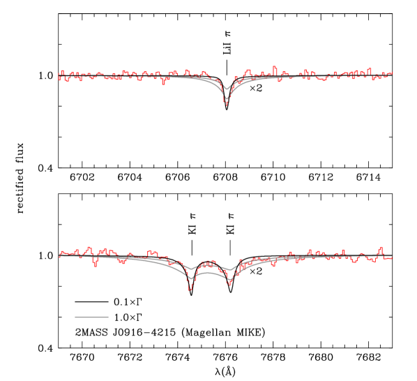
Figure 5: Telluric-corrected MIKE echelle spectrum (red line) for the Li i line (top panel) and K i line (bottom panel) compared to model spectra with broadening parameters at full value (grey line) and divided by 10 (black line). We show again the profiles at full width but with an increased abundance ($\times 2$). The K i $\pi$ doublet appearance is a signature of the Paschen-Back effect at a field of 11.3 MG while Li i $\pi$ achieves a singlet appearance.

Interestingly, Kawka & Vennes (2011), Kawka & Vennes (2014), and Kawka et al. (2019) have already noted that calcium abundance measurements based on Ca i $\lambda$4226, Ca ii H&K, and the Ca ii $\lambda$8578 were often inconsistent. Based on our new results we propose to revise upward the calcium abundance measurement in NLTT 7547 that was presented by Kawka et al. (2019) from $\log{\rm Ca/H}=-10.1$ to $-9.3$, i.e, adjusted to the measurement based on the unsaturated Ca ii $\lambda$8578 line.

Figure 5 shows our analysis of the K i $\lambda$7676 and Li i $\lambda$6707 line profiles. The narrow line shapes were matched by synthetic line profiles including, as noted above, reduced broadening parameters ($\log{\Gamma}-1.0$). The line profiles computed at the same abundance but with the original line broadening parameters obtained from Barklem, Piskunov, & O’Mara (2000b) are clearly too broad and shallow with line wings extending far from the line centre. To show this effect more clearly we also show the full profiles at twice the nominal abundance. The line positions are accurately matched with our Paschen-Back models including the quadratic effect. Their singlet (Li i) and doublet (K i) appearances follow directly from their respective fine-structure energy separation constants $\zeta$ which is much larger in the case of the K i $\lambda$7676 upper level (²P^o) relative to the Li i $\lambda$6707 upper level, $\zeta=$38.5 versus 0.2 cm^-1, or the Na i $\lambda$5891 upper level (see Appendix A.2).

Table 3 lists the resulting abundance measurements by number and Figure 6 shows the corresponding spectral synthesis along with the Magellan echellette (MagE) spectrum (see also Appendix B). We estimate the individual abundance uncertainties at a factor of 2 ($\pm 0.3$ dex). They are dominated by uncertainties in the effective temperature of the star ($\pm 100$ K) and to a lesser extent the uncertainties in the broadening parameters, and the line profile fitting. Therefore, because systematic errors dominate the error budget, errors in abundance ratios should be lower than in individual measurements.

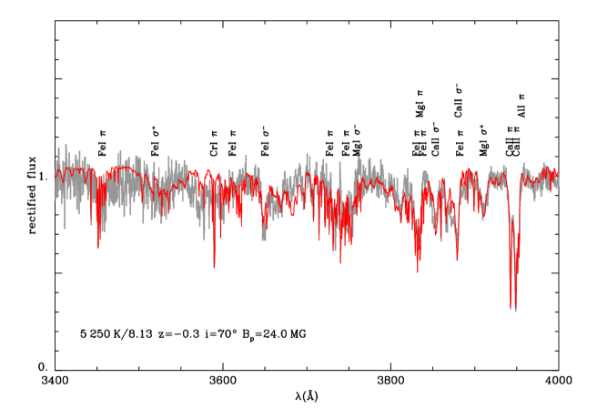
Figure 6: Model spectrum (red line) fitted to the blue side of the MagE echelle spectrum (grey line) using air wavelengths. All spectral lines modelled in this work are marked with the corresponding element and polarization state ($\pi$ or $\sigma_{\pm}$). The complete spectral coverage is presented in Appendix B.

All Ca ii lines belong to the incomplete Paschen-Back regime. The ultraviolet Ca ii lines show the close doublet pattern ($\pi$) as well as split $\sigma_{\pm}$ patterns $\approx\pm 85$Å on both sides and, as expected at $\approx 11.3$ MG (see Equation (1)), a weak vanishing component at $\Delta\lambda\approx+170$Å ($\lambda\approx 4120$Å). The infrared Ca ii sextet shows a corresponding number of $\pi$ components (five are clearly visible in the spectrum and a sixth one is merged with another). The $\sigma_{\pm}$ components of Mg i $\lambda$5178 and Ca i $\lambda$4445 (a sextet at zero field) show a complex triplet structure well matched by the models. Several narrow lines do not have obvious identifications and are shown with "?" marks. A possible identification of a feature near 4480 Å with the excited Mg ii $\lambda$4482 line is problematic because of its high excitation energy and vanishing Boltzmann factor at low temperature.

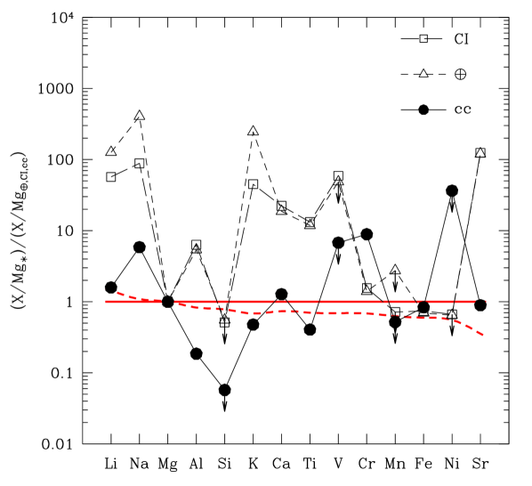
Figure 7: Abundance set in the photosphere of 2MASS J0916$-$4215. The abundance measurements (by number) are normalized to magnesium (${\rm X/Mg_{\ast}}$) and divided by the same measurements in Earth’s continental crust (cc), CI-chondrites (CI), and the bulk Earth composition ($\earth$) as listed in Table 3. Silicon, vanadium, manganese, and nickel abundance upper limits are marked with down arrows. The full red line ($=1$) follows the early build-up assumption, while the dashed red line assumes accretion-diffusion equilibrium (see text).

Figure 7 shows our new abundance measurements listed in Table 3. The abundance measurements are normalized to the magnesium abundance and divided by the corresponding abundance measurements in various bodies and the resulting ratios are plotted for each element. Excluding upper limits (e.g., silicon), the mean and standard deviation of the ratios relative to Earth’s continental crust are $0.05\pm 0.51$, while these values increase to $1.20\pm 0.73$ relative to the CI-chondrites and $1.36\pm 0.94$ relative to the bulk Earth.

The lithium over-abundance in 2MASS J0916$-$4215 approaches $+2$ dex relative to the bulk Earth (McDonough, 2003) or CI-chondrites (Lodders, 2019), but it appears considerably closer to the lithium content of Earth’s (bulk) continental crust (Rudnick & Gao, 2003). The strontium abundance would also point towards a parent body composed of crust-like material. However, the upper limit on the abundance of silicon would imply a large silicon deficit in the parent body assuming Earth’s crust composition. On the other hand, the upper limits on the abundance of vanadium, manganese, and nickel do not help discriminate between the three scenarios. The standard deviation in $\Delta_{\rm cc,Mg}$ measurements is $\approx 0.5$ showing an uncertainty in individual measurements of the order of a factor of 3, or some degrees of variations in the composition of the actual accreted material relative to the estimated composition of crust-like material (Rudnick & Gao, 2003). Oxygen is not detectable in cool white dwarfs such as 2MASS J0916$-$4215, so possible oxide-balance of the accreted material cannot be ascertained (Klein et al., 2010).

3.4 Effect of diffusion: build-up and steady-state regimes

Before any chemical separation takes effect, i.e., at a time following an accretion event much shorter than the diffusion time scale, $t<<\tau$, the abundance pattern (relative to Mg) in the atmosphere replicates the pattern in the accretion flow:

$$\Big{(}\frac{\rm X}{\rm Mg}\Big{)}_{\ast}=\Big{(}\frac{\rm X}{\rm Mg}\Big{)}_{\rm acc}$$ (5)

The comparisons with the full red line depicted in Figure 7 follow this assumption. However, in a steady-state regime at a time $t>>\tau$ when equilibrium is established between diffusion losses at the bottom of the convection zone and the surface resupply, the abundance pattern (relative to Mg) is given by:

$$\Big{(}\frac{\rm X}{\rm Mg}\Big{)}_{\ast}=\Big{(}\frac{\rm X}{\rm Mg}\Big{)}_{\rm acc}\ \frac{\rm\tau(X)}{\rm\tau(Mg)}$$ (6)

where $\tau{\rm(X)}$ is the diffusion time scale for a given element X (or specifically Mg) obtained from the MWDD (Bédard et al., 2020). We note that the mass of the convection zone is calculated assuming that the strong magnetic field has no effect on the depth of the mixed layers in a magnetic white dwarf. The dashed red line in Figure 7 shows mild deviations in the abundance pattern due to diffusion. Assuming either early build-up or steady-state regimes, accretion from a source with crust-like material appears more likely. However, the absence of silicon remains problematic. Moreover, sodium, aluminium and chromium deviate from expected (either in build-up phase or steady-state phase) abundance ratios by more than 0.5 dex. Such large deviations exceed mere statistical errors and may reflect systematic errors in adopted broadening parameter values.

The mass of individual elements accreted onto the star per units of time is given as its mass fraction $Y_{\rm acc}$ of the accretion flow and is expressed in $M_{\odot}\,{\rm yr}^{-1}$ or g s^-1:

$$\dot{M}_{\rm acc,A}=Y_{\rm acc,A}\dot{M}_{\rm acc}=Y_{\rm atm,A}\ \frac{M_{\rm cvz}}{\tau_{\rm A}}$$ (7)

where $A$ identifies an element by its atomic weight, $\dot{M}_{\rm acc}$ is the total mass accreted by units of time, $Y_{\rm atm,A}$ is the mass fraction of element $A$ in the atmosphere, $Y\approx A\,X$, where $X$ is the abundance by number (${\rm X/H}$ in Table 3), $M_{\rm cvz}$ is the mass of the convection zone ($\log{\rm M_{cvz}/M_{\odot}}=-6.33$), and $\tau_{\rm A}$ is the diffusion time-scale of element $A$ at the bottom of the convection zone. Figure 8 shows the diffusion time-scales employed in the calculation of individual accretion rates onto 2MASS J0916$-$4215.

The resulting accretion rates for individual elements are compared to similar rates onto the polluted, magnetic white dwarf NLTT 43806 (Zuckerman et al., 2011). The rates found in 2MASS J0916$-$4215 are a factor of 6 larger than in NLTT 43806 but, otherwise, follow a very similar trend. Zuckerman et al. (2011) concluded that the material accreted onto NLTT 43806 belong to lithosphere-like material (crust and upper mantle). Although the overall abundance pattern in 2MASS J0916$-$4215 would suggest a similar conclusion, the scarcity of aluminium and the absence of silicon indicate that the silicon-rich crust material should be diluted with other types of material. We find that, depending on the adopted scenario, i.e., early build-up phase (equation (6)) or late steady-state phase (equation (7)), individual abundance measurements would vary by at most a factor of 3 due to variations in the diffusion time scales, particularly between lighter and heavier elements. Such mild variations are not readily detectable in our measurements. Therefore, we cannot recover the timeline of accretion events onto 2MASS J0916$-$4215.

Complete or partial suppression of convective mixing could noticeably shorten diffusion time-scales in cool white dwarfs. Following an accretion event the fully convective envelope of a 5 000 K hydrogen-rich white dwarf would retain heavy elements over a time-scale of $\approx 10^{6}$ years, while a radiative photosphere without mixing would retain its composition for merely $\approx 10^{-3}$ years. Unless they are in the process of accreting material, the cool, polluted magnetic white dwarfs would be relatively rare compared to their non-magnetic counterparts. However, an examination of the large sample of polluted, magnetic white dwarfs analyzed by Hollands et al. (2017) and Hollands, Gänsicke, & Koester (2018) shows that the abundance patterns of magnetic and non-magnetic white dwarfs do not differ significantly and that magnetic fields are common among polluted white dwarfs which implies that deep mixing remains effective even among magnetic white dwarfs.

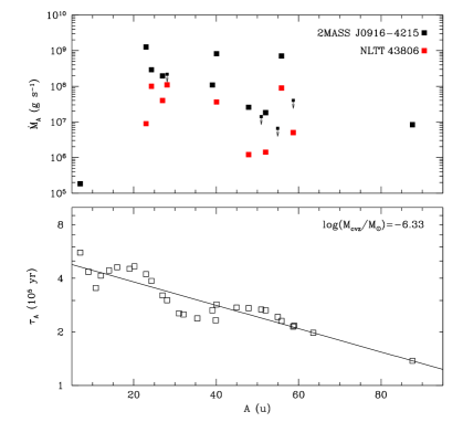
Figure 8: Estimated mass accretion rate (top panel) onto the photosphere of 2MASS J0916$-$4215 (black squares) and NLTT 43806 (red squares, Zuckerman et al., 2011) assuming steady-state equilibrium. Rate upper limits are marked with down arrows. Diffusion time scales (open squares in bottom panel) for a set of elements with atomic weight from $A=6.9$ u (Li) and $A=63.6$ u (Cu) obtained from the MWDD (Bédard et al., 2020). $M_{\rm cvz}$ is the adopted mass of the convection zone expressed as a fraction of the solar mass. The diffusion time scale for strontium ($A=87.6$ u) was estimated by extrapolating available data (full line).

3.5 Kinematics

Using the distance, proper motion and the stellar radial velocity of $\varv=-15\pm 4$ km s^-1, obtained by subtracting a gravitational redshift of 36 km s^-1 from the observed heliocentric radial velocity $\varv_{r}=21$ km s^-1 (see Section 3.2), we calculated the Galactic velocity components relative to the local standard of rest following Johnson & Soderblom (1987). The velocities were corrected for the Solar motion relative to the local standard of rest using ($U_{\odot},V_{\odot},W_{\odot}$) = ($11.10,12.24,7.25$) km s^-1 (Schönrich, Binney, & Dehnen, 2010). The Galactic velocity components of ($U,V,W$) = ($29.3\pm 0.2,25.2\pm 4.0,-7.1\pm 0.3$) km s^-1 place 2MASS J0916$-$4215 in the thin disc.

3.6 Photometric variations

We could not detect any significant photometric variations in 2MASS J0916$-$4215 in the TESS data. Several other cool, magnetic white dwarfs show variations of several hundredth of a magnitude, e.g., NLTT 8435 (Vennes et al., 2018), possibly due to surface field variations or surface elemental abundance variations. However, no surface element abundance changes other than for hydrogen and helium (see, e.g., Caiazzo et al., 2023), as measured with absorption line equivalent widths, have ever been convincingly demonstrated for any white dwarf (e.g., see Section 3.2 in Johnson et al., 2022). With its large element abundances and complex but well-modelled line spectrum, 2MASS J0916$-$4215 would be the ideal candidate for such a study.

4 Discussion and Summary

The intermediate field white dwarf 2MASS J0916$-$4215 is among the first of its class to show spectral lines in the incomplete Paschen-Back regime. Previously, this pattern was observed in the K i spectrum of the lower field DZ white dwarf LHS 2534 (Hollands et al., 2021). The $\pi$ components of several spectral lines show doublet, e.g., Al i $\lambda$3955, K i $\lambda$7676, and Ca ii $\lambda$3945, or triplet appearances characteristic of the incomplete Paschen-Back regime. The infrared Ca ii $\lambda$8578 triplet shows a complex multi-components core structure that falls well into the incomplete Paschen-Back regime. The pattern clearly departs from the anomalous Zeeman effect displayed in several lower-field white dwarfs (Kawka & Vennes, 2011, 2014; Kawka et al., 2019) but it shows split components and residuals of line components that should vanish entirely in the full Pashen-Back regime. We have presented new calculations of the incomplete Paschen-Back regime and listed sample results for the Ca ii H&K doublet. Although we developed a reliable method to adjust broadening parameters in the high density atmosphere of cool white dwarf stars, ab initio calculations of these parameters are needed to help eliminate potential systematic errors in abundance measurements.

To date, lithium has been detected in only seven white dwarfs (Kaiser et al., 2021; Hollands et al., 2021; Elms et al., 2022, this work), including 2MASS J0916$-$4215, all of them cooler than $\approx 5000$ K with the exception of 2MASS J0916$-$4215. Three of them are magnetic which suggests a high incidence of magnetism in cool, polluted white dwarfs (Kawka & Vennes, 2014; Hollands, Gänsicke, & Koester, 2018; Kawka et al., 2019). The lithium to sodium abundance ratio varies from $\log{\rm Li/Na}=-0.1$ to $-3.2$ (in 2MASS J0916$-$4215) but with the five other measurements clustering around $-1.8\pm 0.3$. The material accreted on 2MASS J0916$-$4215 may not be as "differentiated" as the material analyzed by Hollands et al. (2021). The low ionization potential of neutral lithium precludes a detection in warmer objects but a search for this element in objects with temperatures up to 6 000 K should be attempted.

2MASS J0916$-$4215 joins a class of cool, polluted hydrogen-rich white dwarfs as its highest field member ($B_{\rm S}\approx 11.3$ MG, $B_{\rm p}=24$ MG). Pending a definitive model atmosphere analysis, SDSS J1143+6615 (Hollands et al., 2023) could constitute an even higher field member of this class although a hydrogen-rich composition appears unlikely. The spectral energy distribution of 2MASS J0916$-$4215 does not show an excess in the infrared, however the WISE upper limit for the 12$\mu$m flux measurement provides for the possibility of an infrared excess in the mid-infrared range. JWST mid-infrared imaging is needed to investigate the presence of a dusty circumstellar environment. The overall abundance pattern indicates a lithium- and strontium-rich source of material similar to the Earth’s crust but the scarcity of aluminium and silicon argues against this simple interpretation and qualitatively different sources of material are also required.

Data Availability

The MagE and MIKE echelle spectra may be obtained from the authors upon request. These data sets are not currently available on public archives.

Appendix A Incomplete Paschen-Back regime

We revise and expand upon the original calculations presented by Kemic (1975) using methods presented by Cowan (1981), Griffiths (1995), and Landi Degl’Innocenti & Landolfi (2004). In Section A.1 we present our calculations of line strengths and positions for the CaII H&K doublet components under the incomplete Paschen-Back regime, and in Section A.2 we present new results for other spectral lines of interest under the same regime.

We tabulate relevant input data for our calculations in Tables 4 and  5, with the assistance of the NIST Atomic Spectra Database (Kramida et al., 2022). Results of our calculations (line position and strength) for the Ca ii H&K doublet are presented in Tables 6 and  7.

A.1 The Ca II H&K doublet

Kemic (1975) wrote the Hamiltonian for an atom embedded in an external magnetic field as the sum of the spin-orbit, linear Zeeman and quadratic terms:

$${\rm H}={\rm H}_{\rm so}+\beta\,{\rm H}_{\rm B}+\gamma B^{2}\,{\rm H}_{\rm Q}$$ (8)

where $\beta=\mu_{0}B$ and $\mu_{0}=e\hbar/(2m_{e}c)$ is the Bohr magneton acting at a magnetic field strength $B$, and $\gamma=e^{2}/(8m_{e}c^{2})$ is a constant factor applied to the quadratic term ${\rm H_{Q}}$, where all constants have their usual meaning.

In the matrix below, we show the linear Paschen-Back (H_B) matrix elements added to the spin-orbit (H_so) elements for the upper energy levels (4p ²P) of the CaII H&K doublet. The matrix elements due to $H_{B}$ are $g_{L}M\beta$, where $g_{L}=g_{L}(J,L,S)$ is the Lande $g$ value and $M$ the magnetic quantum number, while the matrix elements due to $H_{\rm so}$ describe the level fine-structure. The formulation recovers the anomalous Zeeman effect in the low field limit $\beta<<\zeta$, e.g., $B\lesssim 0.5$ MG for CaII H&K. Here, $\zeta$ is the energy separation constant for a given multiplet, e.g., $\zeta=148.593$ cm^-1 for the CaII 4p configuration. The resulting tri-diagonal matrix structure, $(J,J)$ on the diagonal and, when allowed, $(J,J-1)$ and $(J-1,J)$ off the diagonal, shows the mixed $J$ levels with a common $M$ number at $M=+1/2$ (lines 3 and 4) and $M=-1/2$ (lines 5 and 6) which alters the level structure at higher field:

$$\mathbf{\rm H_{so}+H_{B}}=$$

$$\left(\begin{array}[]{cccccc}\frac{\zeta}{2}+2\beta&0&0&0&0&0\\ 0&\frac{\zeta}{2}-2\beta&0&0&0&0\\ 0&0&\frac{\zeta}{2}+\frac{2\beta}{3}&-\frac{\sqrt{2}}{3}\beta&0&0\\ 0&0&-\frac{\sqrt{2}}{3}\beta&-\zeta+\frac{\beta}{3}&0&0\\ 0&0&0&0&\frac{\zeta}{2}-\frac{2\beta}{3}&-\frac{\sqrt{2}}{3}\beta\\ 0&0&0&0&-\frac{\sqrt{2}}{3}\beta&-\zeta-\frac{\beta}{3}\\ \end{array}\right)$$

These matrix elements are ordered following the state vectors $|SLJM\rangle$, or excluding $SL$ :

$$\hskip 71.13188pt{|J,M\rangle}=\left(\begin{array}[]{c}\frac{3}{2},+\frac{3}{2}\\ \frac{3}{2},-\frac{3}{2}\\ \frac{3}{2},+\frac{1}{2}\\ \frac{1}{2},+\frac{1}{2}\\ \frac{3}{2},-\frac{1}{2}\\ \frac{1}{2},-\frac{1}{2}\\ \end{array}\right)$$

where the numbers $SL$ are in common to all states, e.g., $S=1/2$ and $L=1$ for the Ca ii 4p level. The quadratic matrix elements are obtained following (Kemic, 1975):

$${\rm H_{Q}}=\frac{2}{3}\,\langle SLJM|C_{0}^{(0)}-C_{0}^{(2)}|SLJ^{\prime}M\rangle\ \langle r^{2}\rangle$$ (9)

where $C_{q}^{(k)}$ are operators acting on the state vectors which we solved following Racah (1942) and Cowan (1981). As demonstrated by Kemic (1975) the non-zero matrix elements of the H_Q matrix follow the same tri-diagonal structure described above. Therefore, the following matrix elements are added to the Zeeman and linear Paschen-Back elements:

$$\mathbf{\rm H_{Q}=\langle r^{2}\rangle_{\rm 4p}\,\gamma B^{2}}\left(\begin{array}[]{cccccc}\frac{4}{5}&0&0&0&0&0\\ 0&\frac{4}{5}&0&0&0&0\\ 0&0&\frac{8}{15}&\frac{2\sqrt{2}}{15}&0&0\\ 0&0&\frac{2\sqrt{2}}{15}&\frac{2}{3}&0&0\\ 0&0&0&0&\frac{8}{15}&-\frac{2\sqrt{2}}{15}\\ 0&0&0&0&-\frac{2\sqrt{2}}{15}&\frac{2}{3}\\ \end{array}\right)$$

Figure 9: Fractional line strength as a function of magnetic field in the present work and compared to values tabulated in Kemic (1975). The curves are labelled, from top to bottom in order of appearance, with the corresponding line transition components. The top six line components survive into the full Paschen-Back regime while the lower four components vanish.

The angular part as described by Kemic (1975) includes factors involving the 3-j and 6-j symbols described by Racah (1942) and more recently by Cowan (1981) and Landi Degl’Innocenti & Landolfi (2004), and the matrix elements of spherical harmonics $\langle l||C^{(k)}||l^{\prime}\rangle$ (Racah, 1942; Cowan, 1981). We solved the 3-j and 6-j symbols using fortran subroutines W3JS and W6JS supplied in Landi Degl’Innocenti & Landolfi (2004). The radial part involves the $\langle r^{2}\rangle$ expectation value (mean square radius) for a given configuration:

$$\langle r^{2}\rangle_{nl}=\int r^{2}P_{nl}^{2}(r)dr$$ (10)

where $P_{\rm nl}$ is a normalized radial wave function. Although distinct radial wave functions and $\langle r^{2}\rangle$ expectation values are suggested by Kemic (1975) for the 4p levels P_3/2 and P_1/2 we adopted a single value for the entire upper level configuration, $\langle r^{2}\rangle_{\rm 4p}=22.04$ atomic units (a.u.), while we adopted $\langle r^{2}\rangle_{\rm 4s}=14.84$ a.u. for the lower level configuration. These and other required $\langle r^{2}\rangle$ values for various elements and configurations were computed by us using Cowan et al.’s fortran code RCN following the Hartree-Fock (non-relativistic) scheme.

We note that our H_Q coefficients differ by up to a factor of 2 from those of Kemic (1975) which also appeared inconsistent with each other. The differences do not add up to large deviations in the resulting line wavelengths or strengths due to the relative dominance of the linear Paschen-Back effect in the range of magnetic field considered here ($\lesssim 50$ MG).

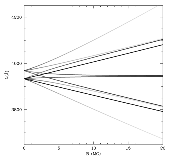
Figure 10: Shifted wavelength positions as a function of magnetic field of the CaII H&K doublet from zero field through the incomplete Paschen-Back regime and towards full Paschen-Back. The line strength is shown from full strength in black through declining strengths using lighter shades of grey towards the full Paschen-Back regime. At this stage, the polarization components $\pi$ and $\sigma_{\pm}$ retain doublet structures.

Applying the selection rule $\Delta M=0,\pm 1$ we recover 10 line components listed in the header of Table 6. After solving for the eigenvalues and eigenvectors of the $\rm H_{so}+H_{B}+H_{Q}$ matrix using the subroutine jacobi supplied in Press, Flannery, & Teukolsky (1986), the wavelength of each component listed in Table 7 was obtained using the calculated energy values:

$$\lambda_{\rm c}=\frac{10^{8}}{(E_{\rm 4p}+E_{\rm up,c})-(E_{\rm 4s}+E_{\rm low,c})}$$ (11)

where $\lambda_{\rm c}$ is given in Å and $c$ designates any of the individual line components $(JM)->(J^{\prime}M^{\prime})$, $E_{\rm up,c}$ is any eigenvalue of the upper level matrix, $E_{\rm 4s}=0$ cm^-1 and $E_{\rm 4p}=25340.10$ cm^-1 are the average configuration energy values recommended by NIST for the lower and upper level of the Ca ii H&K doublet. The energy $E_{\rm low,c}$ belongs to one of the two lower energy levels:

$$E_{\rm low,c}=\pm\mu_{0}B+\frac{2}{3}\langle r^{2}\rangle_{\rm 4s}\,\gamma B^{2}$$ (12)

The wavelengths are converted from vacuum to air.

The method for calculating the strength of each line component is described by Landi Degl’Innocenti & Landolfi (2004). The factors listed in Table 6 are to be applied to the full line strength $S_{ik}$, e.g., $S_{ik}=27$ a.u. for the CaII H&K doublet. Furthermore, the sum of these factors is normalized to unity within each polarization component ($q=0,\pm 1$), i.e., $S_{0}=S_{-1}=S_{+1}=S_{ik}$, so that the sum of the polarization components weighted by the geometrical factors is equal to the total line strength $S_{ik}$:

$$\frac{1}{2}\sin^{2}{\theta}\,S_{0}+\frac{1}{4}(1+\cos^{2}{\theta})\,S_{-1}+\frac{1}{4}(1+\cos^{2}{\theta})\,S_{+1}=S_{ik}$$ (13)

where $\theta$ is the angle between the local magnetic field and the line-of-sight. For the purpose of computing the line opacity, the line strength of each component is converted into an oscillator strength following the relation:

$$gf_{\rm c}=303.754\,\frac{S_{\rm c}}{\lambda_{\rm c}}$$ (14)

where $gf_{\rm c}$ is the product of the statistical weight and oscillator strength and $\lambda_{\rm c}$ is the shifted wavelength for a given component $(JM)->(J^{\prime}M^{\prime})$ and provided in Table 7. Figure 9 compares the results of our line strength calculations to values tabulated in Kemic (1975), but renormalized to $S_{q=0,\pm 1}=1,$ for fields ranging from 0 to 50 MG showing an excellent agreement for all 10 line components although some tabulated values in Kemic (1975) suffer from rounding errors. Figure 10 shows our calculated line position and illustrated line strength for the CaII H&K doublet showing the transition from the anomalous Zeeman regime through the incomplete Paschen-Back regime.

Table 4: Reference data for Paschen-Back calculations of the ²S and ²P^o terms. The configurations $i$ and $k$ designate the lower and upper levels, respectively, while $\zeta$ is the fine-structure energy separation constant, $S_{ik}$ is the total line strength, and $\langle r^{2}\rangle_{i}$ and $\langle r^{2}\rangle_{k}$ are the mean square radii for the lower and upper levels, respectively.

Line	configuration	$\zeta$ (2Po)	$S_{ik}$	$\langle r^{2}\rangle_{i}$	$\langle r^{2}\rangle_{k}$
	$i$ - $k$	(cm-1)	(a.u.)	(a.u.)	(a.u.)
Li i $\lambda$6707	2s - 2p	0.2267	33.0	17.47	27.07
Na i $\lambda$5891	3s - 3p	11.4642	37.3	19.66	40.25
Al i $\lambda$3955a	3p - 4s	74.707	9.05	13.70	64.41
K i $\lambda$7676	4s - 4p	38.474	50.46	28.49	53.02
Ca ii $\lambda$3945	4s - 4p	148.593	27.0	14.84	22.04

^a Symmetric ²P^o - ²S terms.

A.2 Other line transitions in the incomplete Paschen-Back regime

The formulation adopted for the Ca ii H&K doublet can be directly applied to other spectral lines with ²S-²P^o terms such as the Na i $\lambda$5891 doublet. Table 4 lists the atomic data employed to extend the Paschen-Back calculations to these spectral lines. We also employed the formalism of Kemic (1975) to calculate the quadratic Paschen-Back effect in spectral lines with other types of configurations from $L=0$ to 4 (S, P, D, F, H) and total electronic spin from $S=0$ to 3 (Table 5). The linear Paschen-Back matrix elements applicable to these configurations were obtained following the method described by Landi Degl’Innocenti & Landolfi (2004).

In the presence of multiple terms in mixed configurations we computed, when available, the term-dependent $\langle r^{2}\rangle$ values following Condon & Shortley (1935). For example, compare the $\langle r^{2}\rangle$ values in the calcium 3d4p ³F^o, ³D^o, and the ³P^o levels (Table 5). In addition, $\langle r^{2}\rangle$ values proved strongly correlated with the calculated level energy values. Therefore we adjusted the correlation potential factor (Cowan, 1981) to achieve a better match between the calculated energy values and the energy values tabulated at NIST (Kramida et al., 2022).

In the main body of the text we reviewed the accuracy of the theory when confronting our models to high-resolution spectroscopy of the intermediate field white dwarf 2MASS J0916$-$4215. The results were satisfactory in most cases, particularly the ²S - ${}^{2}{\rm P^{o}}$ lines. Comparing the line "center-of-gravity" with the full Paschen-Back calculations of Hollands et al. (2023) shows increasing deviations beyond 20 MG which for the spectral lines considered here would constitute a practical limit to the accuracy of the theory employed in our own calculations. However, the morphology of the Ca ii lines in particular remains far from a simple triplet structure. Since they were computed in zero-field conditions, the mean square radii ($\langle r^{2}\rangle$) remain a major source of uncertainties in computations of the quadratic effect within the present scheme. In addition, failure of the LS-coupling in more complex or mixed electron configurations and uncertainties in Lande-g values also affect the accuracy of the linear Paschen-Back model predictions.

Table 5: Reference data for Paschen-Back calculations of the multiplet or singlet lower ($i$) and upper ($k$) levels. Along with the electronic configurations and associated terms, we include the average lower ($E_{i}$) and upper ($E_{k}$) energy levels, the total line strength ($S_{ik}$), and the mean square radii for the lower and upper levels employed in the quadratic Paschen-Back calculations. We indicate whether a given singlet or multiplet is observed in the spectrum of 2MASS J0916$-$4215.

Element	wavelength	configuration		terms		$E_{i}$	$E_{k}$	$S_{ik}$	$\langle r^{2}\rangle_{i}$	$\langle r^{2}\rangle_{k}$	observed
	(Å)	$i$	$k$	$i$	$k$	(cm-1)	(cm-1)	(a.u.)	(a.u.)	(a.u.)
Na i	8190	3p	3d	2Po	2D	16967.63421	29172.8570	140.	40.25	123.0	Y
Mg i	3835	3s3p	3s3d	3Po	3D	21890.854	47957.042	67.3	19.23	89.78	Y
	5178	3s3p	3s4s	3Po	3S	21890.854	41197.403	20.82	19.23	78.89	Y
Si i	3905	3s23p2	3s23p4s	1S	1Po	15394.370	40991.884	1.17	10.72	80.38	N
Ca i	3637	4s4p	4s5d	3Po	3D	15263.089	42745.620	13.0	29.29	565.6	blend
	4226	4s2	4s4p	1S	1Po	0.000	23652.304	24.4	19.31	43.01	Y
	4300	4s4p	4p2	3Po	3P	15263.089	38507.751	64.0	29.29	29.33	Y
	4445	4s4p	4s4d	3Po	3D	15263.089	37753.738	57.0	29.29	147.2	Y
	5266	3d4s	3d4p	3D	3Po	20356.625	39337.750	39.0	22.41	44.52	Y
	5592	3d4s	3d4p	3D	3Do	20356.625	38232.442	71.0	22.41	43.79	Y
	6142	4s4p	4s5s	3Po	3S	15263.089	31539.495	30.0	29.29	106.8	Y
	6460	3d4s	3d4p	3D	3Fo	20356.625	35831.203	150.0	22.41	40.39	Y
Ca ii	8578	3d	4p	2D	2Po	13686.60	25340.10	21.0	6.835	22.04	Y
Ti i	3646	3d24s2	3d24s4p	a3F	y3Go	222.5141	27639.869	59.7	15.55	36.59	blend
	3743	3d24s2	3d24s4p	a3F	x 3Fo	222.5141	26928.504	33.0	15.55	35.64	blend
	3991	3d24s2	3d24s4p	a3F	y3Fo	222.5141	25267.742	35.2	15.55	33.77	N
	4534	3d34s	3d34p	a5F	y5Fo	6721.393	28767.276	172.	17.93	36.07	Y
	4997	3d34s	3d34p	a5F	y5Go	6721.393	26726.246	185.	17.93	33.48	Y
V i	4392	3d44s	3d44p	a6D	y6Fo	2296.5809	25056.952	190.0	16.37	32.10	N
Cr i	3589	3d54s	3d44s4p	a7S	y7Po	0.000	27847.7433	73.0	15.12	22.43	Y
	4269	3d54s	3d54p	a7S	z7Po	0.000	23415.1784	25.3	15.12	29.17	Y
	5206	3d54s	3d54p	a5S	z5Po	7593.1484	26793.2864	53.2	16.61	33.12	Y
	4350	3d44s2	3d44s4p	a5D	z5Fo	8090.1903	31070.1022	17.0	13.33	23.73	N
	5345	3d44s2	3d54p	a5D	z5Po	8090.1903	26793.2864	9.7	13.33	33.12	N
Mn i	4032	3d54s2	3d54s4p	a6S	z6Po	0.000	24792.42	9.9	12.48	23.01	N
Fe i	3456	3d64s2	3d64s4p	a5D	z5Po	402.961	29329.1731	7.62	11.61	22.63	Y
	3611	3d74s	3d74p	a5F	z5Go	7459.7517	35143.4972	74.6	13.29	28.32	Y
	3727	3d64s2	3d64s4p	a5D	z5Fo	402.961	27219.4636	13.7	11.61	21.69	Y
	3750	3d74s	3d74p	a5F	y5Fo	7459.7517	34117.6793	83.4	13.29	27.28	Y
	3830	3d74s	3d74p	a3F	y3Do	12407.4028	38506.9925	55.4	14.06	32.76	Y
	3838	3d74s	3d74p	a5F	y5Do	7459.7517	33503.7641	45.7	13.29	26.72	Y
	3882	3d64s2	3d64s4p	a5D	z5Do	402.961	26150.7302	7.37	11.61	22.54	Y
	4057	3d74s	3d74p	a3F	y3Fo	12407.4028	37043.8386	68.8	14.06	30.61	Y
	4293	3d74s	3d74p	a3F	z3Go	12407.4028	35690.1840	41.6	14.06	28.94	N
	5059	3d74s	3d64s4p	a5F	z5Fo	7459.7517	27219.4636	0.201	13.29	21.69	N
	5217	3d74s	3d64s4p	a3F	z3Do	12407.4028	31566.8014	3.55	14.06	22.96	N
	5348	3d74s	3d64s4p	a5F	z5Do	7459.7517	26150.7302	3.06	13.29	22.54	N
Ni i	3528	3d94s	3d94p	3D	3Po	731.457	29060.032	21.	11.94	25.14	N
	3566	3d94s	3d94p	1D	1Do	3409.937	31441.635	6.3	12.30	27.59	N
	3619	3d94s	3d94p	1D	1Fo	3409.937	31031.020	11.	12.30	27.09	N
Sr i	4607	5s2	5s5p	1S	1Po	0.000	21698.452	29.1	22.54	50.18	Y

Table 6: Fractional line strength $S$ for each Ca H&K component as a function of the magnetic field strength in the incomplete Paschen-Back regime. Each component is labeled with the quantum numbers $(J,M)$ for the lower level (¹S) and $(J^{\prime},M^{\prime})$ for the upper level (²P), and its membership to the H or K spectral line and grouped within the $\pi$ ($q=0$) or $\sigma_{\pm}$ ($q=\pm 1$) components.

$q$	$-1$				$0$						$+1$
$M,M^{\prime}$	$\frac{1}{2},\frac{3}{2}$	$-\frac{1}{2},\frac{1}{2}$			$\frac{1}{2},\frac{1}{2}$			$-\frac{1}{2},-\frac{1}{2}$			$\frac{1}{2},-\frac{1}{2}$		$-\frac{1}{2},-\frac{3}{2}$
$J,J^{\prime}$	$\frac{1}{2},\frac{3}{2}$	$\frac{1}{2},\frac{3}{2}$	$\frac{1}{2},\frac{1}{2}$		$\frac{1}{2},\frac{3}{2}$	$\frac{1}{2},\frac{1}{2}$		$\frac{1}{2},\frac{3}{2}$	$\frac{1}{2},\frac{1}{2}$		$\frac{1}{2},\frac{3}{2}$	$\frac{1}{2},\frac{1}{2}$	$\frac{1}{2},\frac{3}{2}$
Ca	K	K	H		K	H		K	H		K	H	K
$B$ (MG)	$S$
0.0	0.50000	0.16667	0.33333		0.33333	0.16667		0.33333	0.16667		0.16667	0.33333	0.50000
0.1	0.50000	0.16206	0.33794		0.33794	0.16206		0.32863	0.17137		0.17137	0.32863	0.50000
0.2	0.50000	0.15756	0.34244		0.34244	0.15756		0.32383	0.17617		0.17617	0.32383	0.50000
0.3	0.50000	0.15316	0.34684		0.34684	0.15316		0.31894	0.18106		0.18106	0.31894	0.50000
0.4	0.50000	0.14886	0.35114		0.35114	0.14886		0.31396	0.18604		0.18604	0.31396	0.50000
0.5	0.50000	0.14467	0.35533		0.35533	0.14467		0.30890	0.19110		0.19110	0.30890	0.50000
0.6	0.50000	0.14058	0.35942		0.35942	0.14058		0.30376	0.19624		0.19624	0.30376	0.50000
0.7	0.50000	0.13660	0.36340		0.36340	0.13660		0.29854	0.20146		0.20146	0.29854	0.50000
0.8	0.50000	0.13273	0.36727		0.36727	0.13273		0.29326	0.20674		0.20674	0.29326	0.50000
0.9	0.50000	0.12896	0.37104		0.37104	0.12896		0.28792	0.21208		0.21208	0.28792	0.50000
1.0	0.50000	0.12530	0.37470		0.37470	0.12530		0.28252	0.21748		0.21748	0.28252	0.50000
1.2	0.50000	0.11829	0.38171		0.38171	0.11829		0.27158	0.22842		0.22842	0.27158	0.50000
1.4	0.50000	0.11168	0.38832		0.38832	0.11168		0.26052	0.23948		0.23948	0.26052	0.50000
1.6	0.50000	0.10548	0.39452		0.39452	0.10548		0.24939	0.25061		0.25061	0.24939	0.50000
1.8	0.50000	0.09965	0.40035		0.40035	0.09965		0.23826	0.26174		0.26174	0.23826	0.50000
2.0	0.50000	0.09418	0.40582		0.40582	0.09418		0.22719	0.27281		0.27281	0.22719	0.50000
2.5	0.50000	0.08198	0.41802		0.41802	0.08198		0.20023	0.29977		0.29977	0.20023	0.50000
3.0	0.50000	0.07164	0.42836		0.42836	0.07164		0.17493	0.32507		0.32507	0.17493	0.50000
3.5	0.50000	0.06289	0.43711		0.43711	0.06289		0.15191	0.34809		0.34809	0.15191	0.50000
4.0	0.50000	0.05547	0.44453		0.44453	0.05547		0.13148	0.36852		0.36852	0.13148	0.50000
4.5	0.50000	0.04916	0.45084		0.45084	0.04916		0.11369	0.38631		0.38631	0.11369	0.50000
5.0	0.50000	0.04378	0.45622		0.45622	0.04378		0.09842	0.40158		0.40158	0.09842	0.50000
5.5	0.50000	0.03917	0.46083		0.46083	0.03917		0.08541	0.41459		0.41459	0.08541	0.50000
6.0	0.50000	0.03521	0.46479		0.46479	0.03521		0.07439	0.42561		0.42561	0.07439	0.50000
6.5	0.50000	0.03178	0.46822		0.46822	0.03178		0.06507	0.43493		0.43493	0.06507	0.50000
7.0	0.50000	0.02881	0.47119		0.47119	0.02881		0.05718	0.44282		0.44282	0.05718	0.50000
7.5	0.50000	0.02621	0.47379		0.47379	0.02621		0.05049	0.44951		0.44951	0.05049	0.50000
8.0	0.50000	0.02394	0.47606		0.47606	0.02394		0.04479	0.45521		0.45521	0.04479	0.50000
8.5	0.50000	0.02194	0.47806		0.47806	0.02194		0.03993	0.46007		0.46007	0.03993	0.50000
9.0	0.50000	0.02017	0.47983		0.47983	0.02017		0.03576	0.46424		0.46424	0.03576	0.50000
9.5	0.50000	0.01860	0.48140		0.48140	0.01860		0.03216	0.46784		0.46784	0.03216	0.50000
10.0	0.50000	0.01720	0.48280		0.48280	0.01720		0.02905	0.47095		0.47095	0.02905	0.50000
11.0	0.50000	0.01483	0.48517		0.48517	0.01483		0.02398	0.47602		0.47602	0.02398	0.50000
12.0	0.50000	0.01291	0.48709		0.48709	0.01291		0.02008	0.47992		0.47992	0.02008	0.50000
13.0	0.50000	0.01134	0.48866		0.48866	0.01134		0.01702	0.48298		0.48298	0.01702	0.50000
14.0	0.50000	0.01003	0.48997		0.48997	0.01003		0.01459	0.48541		0.48541	0.01459	0.50000
15.0	0.50000	0.00894	0.49106		0.49106	0.00894		0.01263	0.48737		0.48737	0.01263	0.50000
16.0	0.50000	0.00801	0.49199		0.49199	0.00801		0.01103	0.48897		0.48897	0.01103	0.50000
17.0	0.50000	0.00722	0.49278		0.49278	0.00722		0.00971	0.49029		0.49029	0.00971	0.50000
18.0	0.50000	0.00654	0.49346		0.49346	0.00654		0.00860	0.49140		0.49140	0.00860	0.50000
20.0	0.50000	0.00544	0.49456		0.49456	0.00544		0.00688	0.49312		0.49312	0.00688	0.50000
22.0	0.50000	0.00460	0.49540		0.49540	0.00460		0.00562	0.49438		0.49438	0.00562	0.50000
24.0	0.50000	0.00394	0.49606		0.49606	0.00394		0.00467	0.49533		0.49533	0.00467	0.50000
26.0	0.50000	0.00341	0.49659		0.49659	0.00341		0.00394	0.49606		0.49606	0.00394	0.50000
28.0	0.50000	0.00299	0.49701		0.49701	0.00299		0.00337	0.49663		0.49663	0.00337	0.50000
30.0	0.50000	0.00264	0.49736		0.49736	0.00264		0.00291	0.49709		0.49709	0.00291	0.50000
32.0	0.50000	0.00235	0.49765		0.49765	0.00235		0.00253	0.49747		0.49747	0.00253	0.50000
34.0	0.50000	0.00210	0.49790		0.49790	0.00210		0.00223	0.49777		0.49777	0.00223	0.50000
36.0	0.50000	0.00189	0.49811		0.49811	0.00189		0.00197	0.49803		0.49803	0.00197	0.50000
38.0	0.50000	0.00171	0.49829		0.49829	0.00171		0.00176	0.49824		0.49824	0.00176	0.50000
40.0	0.50000	0.00156	0.49844		0.49844	0.00156		0.00158	0.49842		0.49842	0.00158	0.50000
42.0	0.50000	0.00143	0.49857		0.49857	0.00143		0.00142	0.49858		0.49858	0.00142	0.50000
44.0	0.50000	0.00131	0.49869		0.49869	0.00131		0.00128	0.49872		0.49872	0.00128	0.50000
46.0	0.50000	0.00121	0.49879		0.49879	0.00121		0.00117	0.49883		0.49883	0.00117	0.50000
48.0	0.50000	0.00112	0.49888		0.49888	0.00112		0.00107	0.49893		0.49893	0.00107	0.50000
50.0	0.50000	0.00104	0.49896		0.49896	0.00104		0.00098	0.49902		0.49902	0.00098	0.50000

Table 7: Same as Table 6 but for the air wavelength (in Å) of each Ca H&K component as a function of the magnetic field strength in the incomplete Paschen-Back regime and towards the full regime.

$q$	$-1$				$0$						$+1$
$M,M^{\prime}$	$\frac{1}{2},\frac{3}{2}$	$-\frac{1}{2},\frac{1}{2}$			$\frac{1}{2},\frac{1}{2}$			$-\frac{1}{2},-\frac{1}{2}$			$\frac{1}{2},-\frac{1}{2}$		$-\frac{1}{2},-\frac{3}{2}$
$J,J^{\prime}$	$\frac{1}{2},\frac{3}{2}$	$\frac{1}{2},\frac{3}{2}$	$\frac{1}{2},\frac{1}{2}$		$\frac{1}{2},\frac{3}{2}$	$\frac{1}{2},\frac{1}{2}$		$\frac{1}{2},\frac{3}{2}$	$\frac{1}{2},\frac{1}{2}$		$\frac{1}{2},\frac{3}{2}$	$\frac{1}{2},\frac{1}{2}$	$\frac{1}{2},\frac{3}{2}$
Ca	K	K	H		K	H		K	H		K	H	K
$B$ (MG)	$\lambda_{\rm air}$ (Å)
0.00	3933.66	3933.66	3968.47		3933.66	3968.47		3933.66	3968.47		3933.66	3968.47	3933.66
0.10	3932.94	3932.46	3967.49		3933.90	3968.96		3933.42	3967.98		3934.87	3969.45	3934.39
0.20	3932.22	3931.24	3966.52		3934.13	3969.46		3933.17	3967.50		3936.06	3970.45	3935.11
0.30	3931.50	3930.02	3965.56		3934.36	3969.97		3932.91	3967.03		3937.25	3971.44	3935.83
0.40	3930.77	3928.80	3964.60		3934.57	3970.48		3932.65	3966.56		3938.43	3972.45	3936.56
0.50	3930.05	3927.57	3963.65		3934.79	3971.00		3932.37	3966.11		3939.61	3973.47	3937.28
0.60	3929.33	3926.34	3962.71		3934.99	3971.53		3932.09	3965.66		3940.78	3974.49	3938.00
0.70	3928.61	3925.09	3961.77		3935.19	3972.06		3931.81	3965.21		3941.94	3975.52	3938.73
0.80	3927.89	3923.85	3960.84		3935.39	3972.60		3931.51	3964.78		3943.09	3976.56	3939.45
0.90	3927.17	3922.60	3959.92		3935.58	3973.14		3931.21	3964.35		3944.24	3977.61	3940.17
1.00	3926.45	3921.35	3959.00		3935.76	3973.69		3930.90	3963.93		3945.38	3978.66	3940.90
1.20	3925.00	3918.82	3957.18		3936.11	3974.81		3930.25	3963.12		3947.64	3980.80	3942.35
1.40	3923.56	3916.29	3955.38		3936.45	3975.94		3929.58	3962.34		3949.87	3982.97	3943.80
1.60	3922.12	3913.73	3953.60		3936.76	3977.09		3928.87	3961.59		3952.07	3985.18	3945.25
1.80	3920.68	3911.17	3951.83		3937.06	3978.27		3928.13	3960.87		3954.24	3987.42	3946.70
2.00	3919.24	3908.59	3950.09		3937.34	3979.45		3927.36	3960.19		3956.38	3989.70	3948.15
2.50	3915.64	3902.09	3945.80		3937.97	3982.49		3925.29	3958.62		3961.60	3995.55	3951.78
3.00	3912.05	3895.54	3941.60		3938.53	3985.62		3923.03	3957.24		3966.63	4001.61	3955.41
3.50	3908.46	3888.93	3937.47		3939.01	3988.81		3920.60	3956.04		3971.50	4007.88	3959.05
4.00	3904.88	3882.30	3933.41		3939.44	3992.07		3918.01	3955.01		3976.22	4014.32	3962.69
4.50	3901.29	3875.64	3929.40		3939.82	3995.39		3915.29	3954.11		3980.80	4020.94	3966.33
5.00	3897.71	3868.96	3925.44		3940.16	3998.74		3912.45	3953.33		3985.26	4027.69	3969.98
5.50	3894.14	3862.28	3921.52		3940.46	4002.14		3909.51	3952.66		3989.63	4034.58	3973.63
6.00	3890.57	3855.58	3917.63		3940.73	4005.58		3906.48	3952.08		3993.92	4041.59	3977.29
6.50	3887.00	3848.89	3913.78		3940.98	4009.04		3903.39	3951.57		3998.13	4048.70	3980.95
7.00	3883.44	3842.19	3909.95		3941.20	4012.53		3900.23	3951.13		4002.29	4055.90	3984.61
7.50	3879.88	3835.50	3906.15		3941.40	4016.04		3897.03	3950.73		4006.40	4063.19	3988.28
8.00	3876.32	3828.82	3902.37		3941.59	4019.58		3893.78	3950.39		4010.46	4070.54	3991.95
8.50	3872.77	3822.14	3898.61		3941.76	4023.13		3890.50	3950.08		4014.49	4077.97	3995.62
9.00	3869.22	3815.48	3894.87		3941.91	4026.70		3887.19	3949.81		4018.50	4085.46	3999.30
9.50	3865.67	3808.83	3891.14		3942.06	4030.29		3883.85	3949.57		4022.47	4093.01	4002.98
10.00	3862.13	3802.19	3887.43		3942.20	4033.89		3880.49	3949.35		4026.43	4100.61	4006.66
11.00	3855.06	3788.97	3880.04		3942.44	4041.14		3873.73	3948.97		4034.29	4115.97	4014.04
12.00	3848.00	3775.80	3872.70		3942.66	4048.43		3866.92	3948.67		4042.11	4131.52	4021.44
13.00	3840.95	3762.71	3865.40		3942.85	4055.75		3860.07	3948.41		4049.88	4147.24	4028.85
14.00	3833.92	3749.69	3858.13		3943.02	4063.12		3853.19	3948.20		4057.64	4163.13	4036.28
15.00	3826.91	3736.74	3850.90		3943.18	4070.52		3846.30	3948.02		4065.37	4179.18	4043.72
16.00	3819.91	3723.88	3843.70		3943.32	4077.94		3839.39	3947.87		4073.09	4195.39	4051.17
17.00	3812.92	3711.09	3836.53		3943.46	4085.40		3832.48	3947.74		4080.81	4211.75	4058.64
18.00	3805.95	3698.38	3829.37		3943.58	4092.88		3825.56	3947.63		4088.53	4228.26	4066.13
20.00	3792.05	3673.20	3815.15		3943.82	4107.91		3811.74	3947.46		4103.96	4261.72	4081.14
22.00	3778.20	3648.35	3801.00		3944.02	4123.03		3797.92	3947.35		4119.41	4295.78	4096.22
24.00	3764.41	3623.82	3786.94		3944.22	4138.23		3784.13	3947.27		4134.88	4330.44	4111.35
26.00	3750.68	3599.60	3772.95		3944.41	4153.51		3770.38	3947.22		4150.40	4365.70	4126.54
28.00	3737.01	3575.71	3759.04		3944.58	4168.87		3756.66	3947.20		4165.95	4401.57	4141.80
30.00	3723.39	3552.12	3745.19		3944.76	4184.30		3742.99	3947.20		4181.55	4438.06	4157.11
32.00	3709.83	3528.85	3731.41		3944.93	4199.80		3729.36	3947.22		4197.20	4475.19	4172.49
34.00	3696.33	3505.87	3717.69		3945.10	4215.37		3715.78	3947.26		4212.91	4512.96	4187.92
36.00	3682.88	3483.19	3704.04		3945.27	4231.00		3702.25	3947.31		4228.66	4551.40	4203.42
38.00	3669.49	3460.81	3690.45		3945.44	4246.71		3688.77	3947.37		4244.47	4590.52	4218.97
40.00	3656.16	3438.71	3676.93		3945.61	4262.48		3675.34	3947.45		4260.34	4630.33	4234.59
42.00	3642.88	3416.89	3663.46		3945.79	4278.31		3661.96	3947.54		4276.26	4670.85	4250.26
44.00	3629.65	3395.35	3650.06		3945.97	4294.22		3648.63	3947.64		4292.24	4712.11	4266.00
46.00	3616.48	3374.09	3636.71		3946.16	4310.18		3635.36	3947.75		4308.28	4754.12	4281.80
48.00	3603.37	3353.09	3623.43		3946.34	4326.22		3622.14	3947.88		4324.38	4796.90	4297.66
50.00	3590.31	3332.35	3610.20		3946.53	4342.31		3608.97	3948.01		4340.53	4840.46	4313.57

Appendix B Spectral atlas: MIKE and MagE spectra and spectral synthesis.

The echelle spectra of 2MASS J0916$-$4215 and the spectral synthesis with a wavelength coverage from 4000 to 8800Å are shown in four separate panels in (Fig. 11 and Fig. 12) complementing Figure 6.

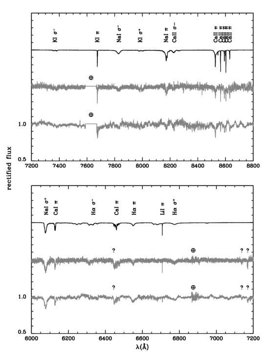
Figure 11: Model spectrum (top black line offset by +1.0), MIKE echelle spectrum (middle grey line offset by +0.5) and MagE echelle spectrum (bottom grey line) using air wavelengths. All spectral lines modelled in this work are marked with the corresponding element and polarization state ($\pi$ or $\sigma_{\pm}$). The question marks ("?") locate unknown features that would not belong to any of the elements identified in the spectrum. Regions affected by telluric absorption are marked with the $\earth$ symbol.

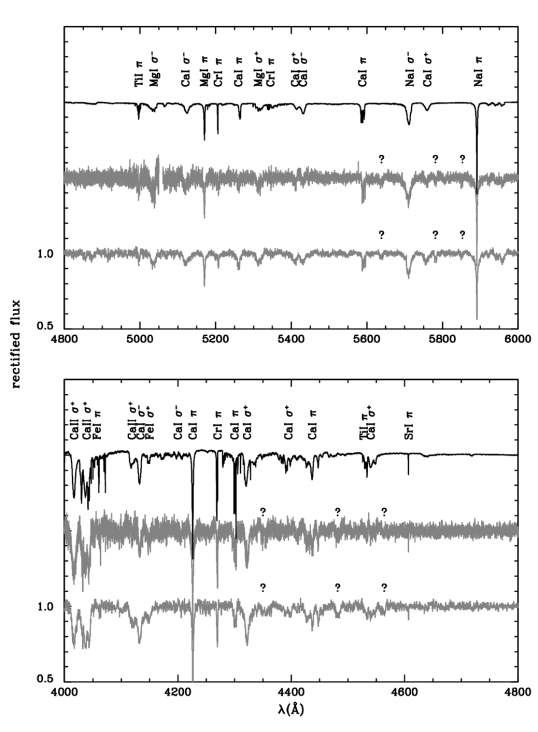
Figure 12: Same as Figure 11 and towards the blue end of the spectra.

References

- Achilleos & Wickramasinghe (1989) Achilleos N., Wickramasinghe D. T., 1989, ApJ, 346, 444. doi:10.1086/168024
- Barklem, Piskunov, & O’Mara (2000a) Barklem P. S., Piskunov N., O’Mara B. J., 2000a, A&A, 363, 1091. doi:10.48550/arXiv.astro-ph/0010022
- Barklem, Piskunov, & O’Mara (2000b) Barklem P. S., Piskunov N., O’Mara B. J., 2000b, A&AS, 142, 467. doi:10.1051/aas:2000167
- Bédard et al. (2020) Bédard A., Bergeron P., Brassard P., Fontaine G., 2020, ApJ, 901, 93. doi:10.3847/1538-4357/abafbe
- Bédard, Bergeron, & Fontaine (2017) Bédard A., Bergeron P., Fontaine G., 2017, ApJ, 848, 11. doi:10.3847/1538-4357/aa8bb6
- Benvenuto & Althaus (1999) Benvenuto O. G., Althaus L. G., 1999, MNRAS, 303, 30. doi:10.1046/j.1365-8711.1999.02215.x
- Bernstein et al. (2003) Bernstein R., Shectman S. A., Gunnels S. M., Mochnacki S., Athey A. E., 2003, SPIE, 4841, 1694. doi:10.1117/12.461502
- Bertaux et al. (2014) Bertaux J. L., Lallement R., Ferron S., Boonne C., Bodichon R., 2014, A&A, 564, A46. doi:10.1051/0004-6361/201322383
- Caiazzo et al. (2023) Caiazzo I., Burdge K. B., Tremblay P.-E., Fuller J., Ferrario L., Gänsicke B. T., Hermes J. J., et al., 2023, Natur, 620, 61. doi:10.1038/s41586-023-06171-9
- Castelli (2005) Castelli F., 2005, MSAIS, 8, 44
- Chayer et al. (1995) Chayer P., Vennes S., Pradhan A. K., Thejll P., Beauchamp A., Fontaine G., Wesemael F., 1995, ApJ, 454, 429. doi:10.1086/176494
- Condon & Shortley (1935) Condon E. U., Shortley G. H., 1935, The Theory of Atomic Spectra, Cambridge: University Press
- Cowan (1981) Cowan, R. D. 1981, The Theory of Atomic Structure and Spectra, Los Alamos Series in Basic and Applied Sciences, Berkeley: University of California Press
- Cunningham et al. (2021) Cunningham T., Tremblay P.-E., Bauer E. B., Toloza O., Cukanovaite E., Koester D., Farihi J., et al., 2021, MNRAS, 503, 1646. doi:10.1093/mnras/stab553
- Cutri et al. (2013) Cutri R. M., et al., 2013, yCat, II/328
- Doyle, Desch, & Young (2021) Doyle A. E., Desch S. J., Young E. D., 2021, ApJL, 907, L35. doi:10.3847/2041-8213/abd9ba
- Doyle et al. (2023) Doyle A. E., Klein B. L., Dufour P., Melis C., Zuckerman B., Xu S., Weinberger A. J., et al., 2023, ApJ, 950, 93. doi:10.3847/1538-4357/acbd44
- Dupuis, Fontaine, & Wesemael (1993) Dupuis J., Fontaine G., Wesemael F., 1993, ApJS, 87, 345. doi:10.1086/191808
- Elms et al. (2022) Elms A. K., Tremblay P.-E., Gänsicke B. T., Koester D., Hollands M. A., Gentile Fusillo N. P., Cunningham T., et al., 2022, MNRAS, 517, 4557. doi:10.1093/mnras/stac2908
- Farihi et al. (2011) Farihi J., Dufour P., Napiwotzki R., Koester D., 2011, MNRAS, 413, 2559. doi:10.1111/j.1365-2966.2011.18325.x
- Gaia Collaboration et al. (2022) Gaia Collaboration, Vallenari A., Brown A. G. A., Prusti T., de Bruijne J. H. J., Arenou F., Babusiaux C., et al., 2022, arXiv, arXiv:2208.00211
- Garstang & Kemic (1974) Garstang R. H., Kemic S. B., 1974, Ap&SS, 31, 103. doi:10.1007/BF00642604
- Gentile Fusillo et al. (2019) Gentile Fusillo N. P., Tremblay P.-E., Gänsicke B. T., Manser C. J., Cunningham T., Cukanovaite E., Hollands M., et al., 2019, MNRAS, 482, 4570. doi:10.1093/mnras/sty3016
- Griffiths (1995) Griffiths, D. J., 1995, Introduction to Quantum Mechanics, Prentice-Hall: Englewood Cliffs
- Hardy, Dufour, & Jordan (2017) Hardy F., Dufour P., Jordan S., 2017, ASPC, 509, 205. doi:10.48550/arXiv.1610.01522
- Hollands, Gänsicke, & Koester (2018) Hollands M. A., Gänsicke B. T., Koester D., 2018, MNRAS, 477, 93. doi:10.1093/mnras/sty592
- Hollands et al. (2017) Hollands M. A., Koester D., Alekseev V., Herbert E. L., Gänsicke B. T., 2017, MNRAS, 467, 4970. doi:10.1093/mnras/stx250
- Hollands et al. (2021) Hollands M. A., Tremblay P.-E., Gänsicke B. T., Koester D., Gentile-Fusillo N. P., 2021, NatAs, 5, 451. doi:10.1038/s41550-020-01296-7
- Hollands et al. (2023) Hollands M. A., Stopkowicz S., Kitsaras M.-P., Hampe F., Blaschke S., Hermes J. J., 2023, MNRAS, 520, 3560. doi:10.1093/mnras/stad143
- Johnson & Soderblom (1987) Johnson D. R. H., Soderblom D. R., 1987, AJ, 93, 864. doi:10.1086/114370
- Johnson et al. (2022) Johnson T. M., Klein B. L., Koester D., Melis C., Zuckerman B., Jura M., 2022, ApJ, 941, 113. doi:10.3847/1538-4357/aca089
- Kaiser et al. (2021) Kaiser B. C., Clemens J. C., Blouin S., Dufour P., Hegedus R. J., Reding J. S., Bédard A., 2021, Sci, 371, 168. doi:10.1126/science.abd1714
- Jura & Young (2014) Jura M., Young E. D., 2014, AREPS, 42, 45. doi:10.1146/annurev-earth-060313-054740
- Kawka & Vennes (2011) Kawka A., Vennes S., 2011, A&A, 532, A7. doi:10.1051/0004-6361/201117078
- Kawka & Vennes (2014) Kawka A., Vennes S., 2014, MNRAS, 439, L90. doi:10.1093/mnrasl/slu004
- Kawka et al. (2019) Kawka A., Vennes S., Ferrario L., Paunzen E., 2019, MNRAS, 482, 5201. doi:10.1093/mnras/sty3048
- Kemic (1975) Kemic S. B., 1975, Ap&SS, 36, 459
- Klein et al. (2021) Klein B. L., Doyle A. E., Zuckerman B., Dufour P., Blouin S., Melis C., Weinberger A. J., et al., 2021, ApJ, 914, 61. doi:10.3847/1538-4357/abe40b
- Klein et al. (2010) Klein B., Jura M., Koester D., Zuckerman B., Melis C., 2010, ApJ, 709, 950. doi:10.1088/0004-637X/709/2/950
- Kramida et al. (2022) Kramida, A., Ralchenko, Yu., Reader, J. and NIST ASD Team, 2022, NIST Atomic Spectra Database (version 5.10), https://physics.nist.gov/asd, National Institute of Standards and Technology, Gaithersburg, MD, DOI: https://doi.org/10.18434/T4W30
- Landi Degl’Innocenti & Landolfi (2004) Landi Degl’Innocenti, E. & Landolfi, M. 2004, Polarization in Spectral Lines, Astrophysics and Space Library Vol. 307, Dordrecht: Kluwer Academic Publishers
- Lodders (2019) Lodders K., 2019, arXiv, arXiv:1912.00844. doi:10.48550/arXiv.1912.00844
- Marocco et al. (2021) Marocco F., Eisenhardt P. R. M., Fowler J. W., Kirkpatrick J. D., Meisner A. M., Schlafly E. F., Stanford S. A., et al., 2021, ApJS, 253, 8. doi:10.3847/1538-4365/abd805
- Marshall et al. (2008) Marshall J. L., Burles S., Thompson I. B., Shectman S. A., Bigelow B. C., Burley G., Birk C., et al., 2008, SPIE, 7014, 701454. doi:10.1117/12.789972
- Martin & Wickramasinghe (1981) Martin B., Wickramasinghe D. T., 1981, MNRAS, 196, 23. doi:10.1093/mnras/196.1.23
- Martin & Wickramasinghe (1984) Martin B., Wickramasinghe D. T., 1984, MNRAS, 206, 407. doi:10.1093/mnras/206.2.407
- McDonough (2003) McDonough W. F., 2003, Treatise on Geochemistry, 2, 568. doi:10.1016/B0-08-043751-6/02015-6
- O’Brien et al. (2023) O’Brien M. W., Tremblay P.-E., Gentile Fusillo N. P., Hollands M. A., Gänsicke B. T., Koester D., Pelisoli I., et al., 2023, MNRAS, 518, 3055. doi:10.1093/mnras/stac3303
- Onken et al. (2019) Onken C. A., Wolf C., Bessell M. S., Chang S.-W., Da Costa G. S., Luvaul L. C., Mackey D., et al., 2019, PASA, 36, e033
- Press, Flannery, & Teukolsky (1986) Press W. H., Flannery B. P., Teukolsky S. A., 1986, Numerical recipes The art of scientific computing, Cambridge: University Press
- Racah (1942) Racah G., 1942, PhRv, 62, 438
- Ricker et al. (2015) Ricker G. R., et al., 2015, JATIS, 1, 014003
- Rudnick & Gao (2003) Rudnick R. L., Gao S., 2003, TrGeo, 3, 659. doi:10.1016/B0-08-043751-6/03016-4
- Schimeczek & Wunner (2014) Schimeczek C., Wunner G., 2014, ApJS, 212, 26. doi:10.1088/0067-0049/212/2/26
- Schönrich, Binney, & Dehnen (2010) Schönrich R., Binney J., Dehnen W., 2010, MNRAS, 403, 1829. doi:10.1111/j.1365-2966.2010.16253.x
- Skrutskie et al. (2006) Skrutskie M. F., Cutri R. M., Stiening R., Weinberg M. D., Schneider S., Carpenter J. M., Beichman C., et al., 2006, AJ, 131, 1163
- Sauval & Tatum (1984) Sauval A. J., Tatum J. B., 1984, ApJS, 56, 193. doi:10.1086/190980
- Tremblay et al. (2015) Tremblay P.-E., Fontaine G., Freytag B., Steiner O., Ludwig H.-G., Steffen M., Wedemeyer S., et al., 2015, ApJ, 812, 19. doi:10.1088/0004-637X/812/1/19
- Vennes et al. (2018) Vennes S., Kawka A., Ferrario L., Paunzen E., 2018, CoSka, 48, 307. doi:10.48550/arXiv.1801.05600
- Veras (2021) Veras, D., 2021, Oxford Research Encyclopedia of Planetary Science, Planetary Systems Around White Dwarfs. Oxford Univ. Press, Oxford, p. 1
- Xu et al. (2014) Xu S., Jura M., Koester D., Klein B., Zuckerman B., 2014, ApJ, 783, 79. doi:10.1088/0004-637X/783/2/79
- Zhao (2018) Zhao L. B., 2018, ApJ, 856, 157. doi:10.3847/1538-4357/aab4fe
- Zuckerman et al. (2007) Zuckerman B., Koester D., Melis C., Hansen B. M., Jura M., 2007, ApJ, 671, 872. doi:10.1086/522223
- Zuckerman et al. (2011) Zuckerman B., Koester D., Dufour P., Melis C., Klein B., Jura M., 2011, ApJ, 739, 101. doi:10.1088/0004-637X/739/2/101
- Zuckerman & Young (2018) Zuckerman B., Young E. D., 2018, haex.book, 14. doi:10.1007/978-3-319-55333-7_14