Occupied Processes: Going with the Flow

Abstract

We develop an Itô calculus for functionals of the ”time” spent by a path at arbitrary levels. A Markovian setting is recovered by lifting a process $X$ with its flow of occupation measures $\operatorname{\mathcal{O}}$ and call the pair $(\operatorname{\mathcal{O}},X)$ the occupied process. While the occupation measure erases the chronology of the path, we show that our framework still includes many relevant problems in stochastic analysis and financial mathematics. The study of occupied processes therefore strikes a middle ground between the path-independent case and Dupire’s Functional Itô Calculus. We extend Itô’s and Feynman-Kac’s formula by introducing the occupation derivative, a projection of the functional linear derivative used extensively in mean field games and McKean-Vlasov optimal control. Importantly, we can recast through Feynman-Kac’s theorem a large class of path-dependent PDEs as parabolic problems where the occupation measure plays the role of time. We apply the present tools to the optimal stopping of spot local time and discuss financial examples including exotic options, corridor variance swaps, and path-dependent volatility.

Keywords: Occupation measure, Itô’s formula, Feynman-Kac theorem, Local

time, Exotic derivatives, Corridor variance swaps, Path-dependent volatility

MSC (2020): 60J55, 60J25, 60H30, 60G40, 91G20

Acknowledgments. I would like to thank Jianfeng Zhang and Bruno Dupire for numerous reflections and discussions. My gratitude goes also to Mete Soner, Jin Ma, Bryan Liang, Felix Hoefer, and the attendees of the Math Finance Colloquium at the University of Southern California in September 2023 for invaluable questions and comments.

1 Introduction

This work originated from an intriguing identity in Revuz and Yor [51, VI, exercise 1.22],

$$\sup_{x}L^{x}_{T}=\sup_{t\leq T}L_{t}^{X_{t}},$$ (1)

where $X$ is standard Brownian motion and $L^{x}$ its local time process at $x$ (see Section 2 for a precise definition). We refer to $L_{t}^{X_{t}}$ as the spot local time. To prove (1), let $x^{*}$ be a maximizer of $x\mapsto L^{x}_{T}$ and define the random time $\tau^{*}=\sup\{t\leq T\ |\ X_{t}=x^{*}\}$. Then $\sup_{x}L^{x}_{T}=L_{\tau^{*}}^{X_{\tau^{*}}}$, which shows that $\sup_{x}L^{x}_{T}\leq\sup_{t\leq T}L_{t}^{X_{t}}$. The reversed inequality is immediate. One question arises: what if we replace the anticipative strategy $\tau^{*}$ by stopping times? In other words, what is the optimal rule and value of the optimal stopping (OS) problem,

$$\sup\{\operatorname{\mathbb{E}}[L_{\tau}^{X_{\tau}}]\ \mathrel{\mathop{\ordinarycolon}}\ \tau=\text{stopping time}\}?$$ (2)

Figure 1: Illustration of (1). The horizontal and vertical bars depicts respectively the local time over $[0,T]$ across levels (left-hand side) and spot local time (right-hand side).

Before solving path-dependent OS problems, it is wise to check if a tractable Markovian framework can be recovered. Indeed, this considerably simplifies the analysis of optimal stopping problems (see, e.g., [50]) and eventual numerical implementation. In our context, we exploit the well-known fact that for continuous semimartingales, the local time field $(L_{t}^{x})_{x\in\operatorname{\mathbb{R}}}$ coincides almost surely with the Radon-Nikodym derivative of the occupation measure,

$$\operatorname{\mathcal{O}}_{t}(A)=\int_{0}^{t}\mathds{1}_{A}(X_{s})d\langle X\rangle_{s},\quad A=\text{Borel set in }\operatorname{\mathbb{R}}.$$ (3)

See [34], [51, Chapter VI], and Section 2.1. The random flow $\operatorname{\mathcal{O}}$ is a measure-valued process adapted to the filtration of $X$. Due to its time additivity recalled in Proposition 1, it is easily shown that the occupied process $(\operatorname{\mathcal{O}},X)$ is Markov as soon as $X$ itself is Markov.

The goal of this work is to develop a differential calculus for occupied processes and demonstrate its relevance and practicality. As occupation measures lose track of the chronology of paths (see Section 2.3), the study of occupied processes strikes a middle ground between the classical Itô calculus and the fully path-dependent setting introduced by Dupire [28]. We shall see throughout that numerous examples in stochastic analysis and financial mathematics still fit into our framework. Moreover, the occupation measure gives rise to nice structural and regularity properties otherwise unavailable in pathwise calculi.

Introduced by Dawson [23, 24] and Fleming and Viot [33], measure-valued processes have gained increasing attention recently, e.g., in mean field games and McKean-Vlasov controls [15, 16, 44, 53, 54], robust pricing and hedging [18, 19], and infinite-dimensional polynomial diffusions [20, 22]. The measure may represent the marginal law of a process or a conditional distribution which concentrates as the filtration unfolds [18, 19]. Either way, the process takes values in a suitable subspace of probability measures. In contrast, $\operatorname{\mathcal{O}}$ evolves in the convex cone $\operatorname{\mathcal{M}}$ of finite measures. The meaning behind the occupation measure also greatly differs from flows of distributions: it is a pathwise object whose total mass increases with the passage of time. Besides, occupation measures can be added to one another. To study occupation functionals, this presents in passing a clear advantage over working in the path space, deprived of vector space structure.

To our best knowledge, functionals of occupied processes and their dynamics have not been studied in the present literature. In fact, the occupation measure is rarely the main object of interest and comes rather as a tool. For instance, let us mention the use of the expected occupation measure to formulate relaxed optimal stopping or stochastic control problems [8, 13, 32]. Herein, the occupation measure is in contrast given at the outset, and may directly appear in the objective function of control problems as exemplified by the optimal stopping of spot local time in Section 4.

Contributions. In Theorem 3.1, we generalize Itô’s formula to occupation functionals $f=f(\operatorname{\mathcal{O}}_{t},X_{t})$ and discover, to our fortunate surprise, that the expression is almost identical to the classical case. The only difference is that the usual time derivative in Itô’s formula for functions $f=f(t,X_{t})$ is replaced by the occupation derivative $\partial_{o}f(\operatorname{\mathcal{O}}_{t},X_{t})=\delta_{\mu}f(\operatorname{\mathcal{O}}_{t},X_{t})(X_{t})$ where $\delta_{\mu}$ is the functional linear derivative [15, Chapter 2]. The projection of $\delta_{\mu}f(\operatorname{\mathcal{O}}_{t},X_{t})\in\operatorname{\mathcal{C}}(\operatorname{\mathbb{R}})$ onto the spot value $X_{t}$ comes from the singular dynamics of the occupation measure. Indeed, it is straightforward to show (see Section 3.1) that

$$d\operatorname{\mathcal{O}}_{t}=\delta_{X_{t}}d\langle X\rangle_{t},\qquad\delta_{X_{t}}=\text{Dirac mass at }X_{t}.$$

We are then able to extend Itô’s formula to occupied continuous semimartingales, namely

$$df(\operatorname{\mathcal{O}}_{t},X_{t})=\Big{(}\partial_{o}+\frac{1}{2}\partial_{xx}\Big{)}f(\operatorname{\mathcal{O}}_{t},X_{t})d\langle X\rangle_{t}+\partial_{x}f(\operatorname{\mathcal{O}}_{u},X_{t})dX_{t}.$$ (4)

See Theorem 3.1. The celebrated occupation time formula $\int_{0}^{t}\phi(X_{s})d\langle X\rangle_{s}=\int_{\operatorname{\mathbb{R}}}\phi d\operatorname{\mathcal{O}}_{t}$ [51, Chapter VI] turns out to be a powerful tool to prove (4) and other results throughout. In Section 3.2.1, we show that (4) is consistent with the functional Itô formula introduced by Dupire [28]. Precisely, the occupation derivative $\partial_{o}$ plays the same role as the functional time derivative in some situations. We also draw in Section 3.2.2 a parallel between the Malliavin derivative (see, e.g., [26]) and the mixed term $\partial_{xo}f(\operatorname{\mathcal{O}}_{t},X_{t})$, akin to the Lions derivative in mean field games [44, 16].

In Section 3.3, we prove a Feynman-Kac type theorem for occupied Brownian motion. Loosely speaking, it states that $v\mathrel{\mathop{\ordinarycolon}}\operatorname{\mathcal{M}}\times\operatorname{\mathbb{R}}\to\operatorname{\mathbb{R}}$ solves the backward heat equation,

$$\Big{(}\partial_{o}+\frac{1}{2}\partial_{xx}\Big{)}v(o,x)=0,\;\ o(\operatorname{\mathbb{R}})<T,\qquad v(o,x)=\varphi(o,x),\;\ o(\operatorname{\mathbb{R}})=T,$$

if and only if $v(o,x)=\operatorname{\mathbb{E}}^{\operatorname{\mathbb{Q}}}_{o,x}[\varphi(\operatorname{\mathcal{O}}_{T},X_{T})]$ for fixed horizon $T>0$. As the total mass satisfies $\operatorname{\mathcal{O}}_{t}(\operatorname{\mathbb{R}})=t$ for Brownian motion, the terminal condition is easily characterized by the pairs $(o,x)$ such that $o(\operatorname{\mathbb{R}})=T$. This is no longer the case for general processes, including solutions of occupied stochastic differential equations (OSDEs, see Section 3.4),

$$d\operatorname{\mathcal{O}}_{t}=\delta_{X_{t}}\sigma(\operatorname{\mathcal{O}}_{t},X_{t})^{2}dt,\qquad dX_{t}=b(\operatorname{\mathcal{O}}_{t},X_{t})dt+\sigma(\operatorname{\mathcal{O}}_{t},X_{t})dW_{t}.$$ (5)

The ambiguity in the terminal condition is removed by defining $v(o,x)=\operatorname{\mathbb{E}}^{\operatorname{\mathbb{Q}}}_{o,x}[\varphi(\operatorname{\mathcal{O}}_{\tau_{\Theta}},X_{\tau_{\Theta}})]$ where $\tau_{\Theta}$ is the exit time of $\operatorname{\mathcal{O}}$ from the ball $\operatorname{\mathcal{M}}_{\Theta}=\{o\in\operatorname{\mathcal{M}}\mathrel{\mathop{\ordinarycolon}}o(\operatorname{\mathbb{R}})<\Theta\}$ for some total mass budget $\Theta>0$. If $(\operatorname{\mathcal{O}},X)$ solves (5), this gives the Dirichlet problem,

$$\Big{(}\sigma^{2}\partial_{o}+b\partial_{x}+\frac{\sigma^{2}}{2}\partial_{xx}\Big{)}v(o,x)=0,\;\ o\in\operatorname{\mathcal{M}}_{\Theta},\qquad v(o,x)=\varphi(o,x),\;\ o\in\partial\!\operatorname{\mathcal{M}}_{\Theta}.$$ (6)

We can therefore recast a large class of path-dependent PDEs as parabolic Dirichlet problems involving the occupation derivative $\partial_{o}$ in lieu of $\partial_{t}$. An even closer connection to parabolic problems emerges when $\operatorname{\mathcal{O}}$ is replaced by the standard time occupation measure,

$$\tilde{\operatorname{\mathcal{O}}}_{t}(A)=\int_{0}^{t}\mathds{1}_{A}(X_{s})ds,$$ (7)

where the first equation in (6) becomes $(\partial_{o}+b\partial_{x}+\frac{\sigma^{2}}{2}\partial_{xx})v=0$. We anticipate that our framework allows to leverage classical results in viscosity theory to a large class of (nonlinear) parabolic path-dependent PDEs, especially those of the form $\partial_{o}v+H(o,x,v,\nabla_{x}v,\nabla_{x}^{2}v)=0$ arising from stochastic optimal control problems [31].

Proving the regularity of solutions of path-dependent PDEs is notoriously hard [56, Chapter 11], [49, 30] and still a subject of active research. In a recent work, Bouchard and Tan [11] study linear parabolic PPDEs for functionals depending on $X_{t}$ and $I_{t}=\int_{0}^{t}X_{s}dA_{s}$ for some continuous function $A$ of finite variation. Note that their setting relates to ours as the integral process $I$ can be retrieved from the occupation measure in some situations. Indeed, if $A_{t}\mathrel{\mathop{\ordinarycolon}}=\langle X\rangle_{t}$ is deterministic (e.g., when $X$ is a Gaussian martingale) and fulfills the conditions in [11], then $I_{t}=\int_{\operatorname{\mathbb{R}}}x\operatorname{\mathcal{O}}_{t}(dx)$.

In path-dependent problems, choosing the right state enlargement is crucial towards the regularity (and tractability for numerical methods) of the Markovian representation of conditional expectations such as $v(\operatorname{\mathcal{O}}_{t},X_{t})=\operatorname{\mathbb{E}}^{\operatorname{\mathbb{Q}}}[\varphi(\operatorname{\mathcal{O}}_{T},X_{T})|\operatorname{\mathcal{F}}_{t}]$; see Viens and Zhang [55] in the context of Gaussian Volterra processes or the ”Better Asian PDE” example in [28]. While one can always define the path functional,

$$V(X)=\operatorname{\mathbb{E}}^{\operatorname{\mathbb{Q}}}[\varphi(\operatorname{\mathcal{O}}_{T},X_{T})|\operatorname{\mathcal{F}}_{t}],\quad X=(X_{s})_{s\in[0,t]},$$

which trivially induces a Markovian framework, even the continuity of $V$ is typically not guaranteed: we shall see in Example 6 related to spot local times that $V$ is discontinuous in the input path while $v$ is smooth, further supporting the choice of the lift $(\operatorname{\mathcal{O}},X)$.

Applications. The spot local time OS problem (2) is at last analyzed in Section 4. After extending standard tools in optimal stopping to our context, we shed light in Section 4.3 on the numerical resolution of (2) by demonstrating an intuitive stopping rule and a least square Monte Carlo approach similar to [48]. The stopping of spot local time reveals great challenges numerically and come across as a novel benchmark for numerical methods solving path-dependent OS problems such as [3, 4, 5]. In Section 4.4, the inevitable approximation of local time $L_{t}^{x}\approx\frac{\operatorname{\mathcal{O}}_{t}((x-\varepsilon,x+\varepsilon))}{2\varepsilon}$ in numerical algorithms is backed up by convergence results for the value of (2) as the width $\varepsilon$ shrinks to zero.

Section 5 is dedicated to financial examples. We shall see that occupation functionals are ever-present, particularly in the eponymous occupation time derivatives [25, 42, 17], timer options, and corridor variance swaps. In some situations, it proves useful to replace $\operatorname{\mathcal{O}}$ by the standard time occupation $\tilde{\operatorname{\mathcal{O}}}$ measure seen in (7). Examples include Asian options contingent upon the time average $\frac{1}{t}\int_{0}^{t}X_{s}ds=\frac{1}{\tilde{\operatorname{\mathcal{O}}}_{t}(\operatorname{\mathbb{R}})}\int_{\operatorname{\mathbb{R}}}xd\tilde{\operatorname{\mathcal{O}}}_{t}$ or Parisian options depending on the actual time that the underlying asset spent above/below a barrier; see [17, 42], and Example 9. In Example 10, we propose yet another variation of the occupation measure, namely $\operatorname{\mathcal{O}}_{t}^{\kappa}(A)=\int_{0}^{t}\mathds{1}_{A}(X_{s})e^{\kappa s}ds$, $\kappa>0$. Noting that,

$$\frac{1}{\mathcal{O}^{\kappa}_{t}(\mathbb{R})}\int x\ \mathcal{O}^{\kappa}_{t}(dx)=\frac{1}{1-e^{-\kappa t}}\int_{0}^{t}X_{u}\kappa e^{-\kappa(t-u)}du,$$

then $\operatorname{\mathcal{O}}^{\kappa}$ incorporates an exponential decay into the occupation measure, which is of great relevance in path-dependent volatility models [36, 37, 39, 41] as we shall see in Section 5.4.

2 Occupied Processes

Unless stated otherwise, every process $X,W,\ldots$ takes values in $\operatorname{\mathbb{R}}$ to simplify the exposition.

Notations. Let $\lambda$ be the Lebesgue measure on $\operatorname{\mathbb{R}}$. We may write $\int fd\lambda$ or $\int f(x)dx$, whichever is more convenient. We also write $\operatorname{\mathcal{B}}(\operatorname{\mathbb{R}})$ for the Borel $\sigma-$algebra on $\operatorname{\mathbb{R}}$ and $\operatorname{\mathcal{M}}$ for the set of finite Radon measures $\mu\mathrel{\mathop{\ordinarycolon}}\operatorname{\mathcal{B}}(\operatorname{\mathbb{R}})\to[0,\infty)$. Given $\mu\in\operatorname{\mathcal{M}}$, $\mathop{\,\,\hbox to0.0pt{--\hss}\int}\nolimits_{A}fd\mu=\frac{1}{\mu(A)}\int_{A}fd\mu$ denotes the average of $f$ with respect to $\mu$ inside $A\in\operatorname{\mathcal{B}}(\operatorname{\mathbb{R}})$. We also write $B_{\varepsilon}=(-\varepsilon,\varepsilon)$ for the open ball of radius $\varepsilon$ centered at the origin and $B_{\varepsilon}(x)=x+B_{\varepsilon}$. Finally, int$A$, $\partial A$, $\bar{A}$ denote the interior, boundary, and closure of a set $A$, respectively.

2.1 Occupation Measure

Given $T\in(0,\infty)$, let $X$ be a real-valued continuous semimartingale on a probability space $(\Omega,\operatorname{\mathcal{F}},\operatorname{\mathbb{F}},\operatorname{\mathbb{Q}})$ where $\operatorname{\mathbb{F}}=(\operatorname{\mathcal{F}}_{t})_{t\leq T}$ is the natural filtration of $X$. The occupation measure of $X$ at $t\in[0,T]$ is defined as

$$\operatorname{\mathcal{O}}_{t}(\omega)\mathrel{\mathop{\ordinarycolon}}\operatorname{\mathcal{B}}(\operatorname{\mathbb{R}})\to\operatorname{\mathbb{R}},\quad\operatorname{\mathcal{O}}_{t}(\omega)(A)=\int_{0}^{t}\mathds{1}_{A}(X_{u})d\langle X\rangle_{u}(\omega),\quad A\in\operatorname{\mathcal{B}}(\operatorname{\mathbb{R}}),\;\omega\in\Omega.$$ (8)

For brevity, we shall omit the dependence on the atom $\omega$ throughout and write $\operatorname{\mathcal{O}}_{t}(A)$ for the random variable $\omega\mapsto\operatorname{\mathcal{O}}_{t}(\omega)(A)$. The flow $\operatorname{\mathcal{O}}=(\operatorname{\mathcal{O}}_{t})_{t\leq T}$ is a measure-valued process [23, 24, 33] adapted to $\operatorname{\mathbb{F}}$ and satisfies useful properties. We collect some of them in the next proposition.

Proposition 1.

The flow of occupation measures $\operatorname{\mathcal{O}}$ satisfies the following properties.

• (Strong Time Additivity) For all stopping times $\varsigma\leq\tau$ and $A\in\operatorname{\mathcal{B}}(\operatorname{\mathbb{R}})$, then

  $$\operatorname{\mathcal{O}}_{\tau}(A)=\operatorname{\mathcal{O}}_{\varsigma}(A)+\operatorname{\mathcal{O}}_{\varsigma,\tau}(A),\quad\operatorname{\mathbb{Q}}-a.s.,$$ (9)

  with the incremental measure $\operatorname{\mathcal{O}}_{s,t}(A)\mathrel{\mathop{\ordinarycolon}}=\int_{s}^{t}\mathds{1}_{A}(X_{u})d\langle X\rangle_{u}$, $s\leq t$.

• (Absolute Continuity) $\operatorname{\mathcal{O}}_{t}\ll\lambda$ $\ \operatorname{\mathbb{Q}}-$a.s. ($\lambda=$ Lebesgue measure on $\operatorname{\mathbb{R}}$).

• (Occupation Time Formula) For every positive Borel function $\phi\mathrel{\mathop{\ordinarycolon}}\operatorname{\mathbb{R}}\to\operatorname{\mathbb{R}}_{+}$,

  $$\int_{0}^{t}\phi(X_{u})d\langle X\rangle_{u}=\int_{\operatorname{\mathbb{R}}}\phi(x)\operatorname{\mathcal{O}}_{t}(dx).$$ (10)

Proof.

See I. [51, X]; II. [51, VI] or [34]; III. [51, VI]. ∎

The Radon-Nikodym derivative of $\operatorname{\mathcal{O}}_{t}$ is the celebrated local time $L_{t}=(L_{t}^{x})_{x\in\operatorname{\mathbb{R}}}$ at $t$, namely

$$L_{t}^{x}=\frac{d\operatorname{\mathcal{O}}_{t}}{d\lambda}(x)=\lim_{\varepsilon\to 0}\frac{1}{2\varepsilon}\int_{0}^{t}\mathds{1}_{B_{\varepsilon}(x)}(X_{u})d\langle X\rangle_{u}.$$ (11)

Therefore, the occupation time formula (10) can be rewritten as

$$\int_{0}^{t}\phi(X_{u})d\langle X\rangle_{u}=\int_{\operatorname{\mathbb{R}}}\phi(x)L_{t}^{x}dx.$$ (12)

Evidently, the time additivity of $\operatorname{\mathcal{O}}$ (Proposition 1 I.) carries over to $L$, that is $L_{t}=L_{s}+L_{s,t}$ with $L_{s,t}\mathrel{\mathop{\ordinarycolon}}=\frac{d\operatorname{\mathcal{O}}_{s,t}}{d\lambda}$. The local time is in fact central in in the theory of additive functionals [9], [51, Chapter X]. For local martingales, it is well-known that the process $L_{t}=(L_{t}^{x})_{x\in\operatorname{\mathbb{R}}}$ (indexed by $x$) admits a version that is $\alpha-$Hölder continuous for all $\alpha<1/2$. For general semimartingales, $x\mapsto L_{t}^{x}$ may only shown to be càdlàg [51, Chapter VI]. Finally, note that $\operatorname{\mathcal{O}}_{t}(\operatorname{\mathbb{R}})=\int_{\operatorname{\mathbb{R}}}L_{t}d\lambda=\langle X\rangle_{t}$, i.e., the total mass of the flow $\operatorname{\mathcal{O}}$ coincides with the stochastic clock $\langle X\rangle$ of $X$.

Let $L_{0}^{\infty}(\operatorname{\mathbb{R}})$ be the subspace of bounded, compactly supported functions on $\operatorname{\mathbb{R}}$, and recall that $\operatorname{\mathcal{M}}$ consists of all finite Radon measures on $\operatorname{\mathbb{R}}$. Introduce the subspace,

$$\operatorname{\mathcal{M}}^{\lambda}=\left\{o\in\operatorname{\mathcal{M}}\ \mathrel{\mathop{\ordinarycolon}}\ o\ll\lambda,\;\frac{do}{d\lambda}\in L_{0}^{\infty}(\operatorname{\mathbb{R}})\right\}.$$ (13)

Clearly, $\operatorname{\mathcal{O}}_{t}\in\operatorname{\mathcal{M}}^{\lambda}\ \operatorname{\mathbb{Q}}-$a.s. from Proposition 1 II. and the compactness of $\{X_{s}\mathrel{\mathop{\ordinarycolon}}s\leq t\}=\text{supp}(\operatorname{\mathcal{O}}_{t})$ as $X$ is continuous. Note that $\operatorname{\mathcal{M}}^{\lambda}$ (or more generally $\operatorname{\mathcal{M}}$) is a convex cone. In particular, occupation measures can be added to one another, as seen in (9). This vector space feature of $\operatorname{\mathcal{M}}^{\lambda}$ is advantageous over a pathwise setting where the addition of paths on different horizons cannot be reasonably defined.

Remark 1.

It is sometime adequate to consider the standard time occupation measure,

$$\tilde{\operatorname{\mathcal{O}}}_{t}(A)\mathrel{\mathop{\ordinarycolon}}=\int_{0}^{t}\mathds{1}_{A}(X_{u})du,\quad A\in\operatorname{\mathcal{B}}(\operatorname{\mathbb{R}}),$$ (14)

or more generally $\tilde{\operatorname{\mathcal{O}}}_{t}(A)\mathrel{\mathop{\ordinarycolon}}=\int_{0}^{t}\mathds{1}_{A}(X_{u})\mu(du)$ for some deterministic measure $\mu$ on $[0,\infty)$, e.g. $\mu(du)=e^{\kappa u}du$; see Example 10. The flow $\tilde{\operatorname{\mathcal{O}}}$ also satisfies properties I., III. in Proposition 1, but not II. Indeed, $\tilde{\operatorname{\mathcal{O}}}$ may generate atoms if $X$ is constant on a time interval of positive length. Hence $\tilde{\operatorname{\mathcal{O}}}_{t}\in\operatorname{\mathcal{M}}\setminus\operatorname{\mathcal{M}}^{\lambda}$ in general, so there may not exist an associated local time process. On the other hand, the standard time occupation measure is well-defined for paths of any roughness and nontrivial for smooth trajectories. Therefore, $\tilde{\operatorname{\mathcal{O}}}$ is more universal than $\operatorname{\mathcal{O}}$ and may be preferred in some financial applications; see Sections 5.1 and 5.4.

Metrics on $\operatorname{\mathcal{M}}^{\lambda}$. We exploit the absolute continuity of elements in $\operatorname{\mathcal{M}}^{\lambda}$ to define the following metrics induced by their respective Radon-Nikodym derivatives, namely

$$\operatorname{\mathfrak{m}}_{p}(o,o^{\prime})\mathrel{\mathop{\ordinarycolon}}=\lVert o-o^{\prime}\rVert_{p},\quad\lVert o\rVert_{p}\mathrel{\mathop{\ordinarycolon}}=\left\lVert\frac{do}{d\lambda}\right\rVert_{L^{p}(\operatorname{\mathbb{R}})},\quad o,o^{\prime}\in\operatorname{\mathcal{M}}^{\lambda},\quad p\in[1,\infty].$$ (15)

Since $\frac{do}{d\lambda}$ is bounded and compactly supported for each $o\in\operatorname{\mathcal{M}}^{\lambda}$, we gather that $\lVert o\rVert_{p}<\infty$ $\forall\ p\in[1,\infty]$. Notice also that $(\operatorname{\mathcal{M}}^{\lambda},\lVert\cdot\rVert_{p})$ is a Banach space, being isometrically isomorphic to $(L_{0}^{\infty}(\operatorname{\mathbb{R}}),\lVert\cdot\rVert_{L^{p}(\operatorname{\mathbb{R}})})$ for each $p\in[1,\infty]$. Note that the distance between any two measures $\operatorname{\mathcal{M}}^{\lambda}$ makes sense irrespective of their respective total mass. This is particularly convenient when comparing the occupation measure at different times, to wit,

$$\operatorname{\mathfrak{m}}_{p}(\operatorname{\mathcal{O}}_{s},\operatorname{\mathcal{O}}_{t})=\lVert\operatorname{\mathcal{O}}_{s,t}\rVert_{p}=\lVert L_{s,t}\rVert_{L^{p}(\operatorname{\mathbb{R}})},\quad s<t.$$

Important values for $p$ are $p\in\{1,2,\infty\}$ as we now explain.

$\bm{p=1}$. Then $\operatorname{\mathfrak{m}}_{1}$ coincides with the total variation distance of finite measures, so it can be generalized to $\operatorname{\mathcal{M}}$. Moreover, for all $o,\Delta\in\operatorname{\mathcal{M}}$, observe that $\operatorname{\mathfrak{m}}_{1}(o,o+\Delta)=\lVert\Delta\rVert_{1}$ is precisely the total mass of $\Delta$. For these reasons, $\operatorname{\mathfrak{m}}_{1}$ will be our choice in Section 3 when establish Itô’s formula for both the occupation measure $\operatorname{\mathcal{O}}$ and the standard time version $\tilde{\operatorname{\mathcal{O}}}$.

$\bm{p=2}$. Note that $(o,o^{\prime})\mathrel{\mathop{\ordinarycolon}}=\big{(}\frac{do}{d\lambda},\frac{do^{\prime}}{d\lambda}\big{)}_{L^{2}(\operatorname{\mathbb{R}})}$ induces a Hilbert structure on $\operatorname{\mathcal{M}}^{\lambda}$ and a natural notion of (Fréchet) differentiability for maps $f\mathrel{\mathop{\ordinarycolon}}\operatorname{\mathcal{M}}^{\lambda}\to\operatorname{\mathbb{R}}$; see Remark 3. Besides, a correspondence can be obtained between $(\operatorname{\mathcal{M}}^{\lambda},(\cdot,\cdot))$ and the Cameron-Martin space $\operatorname{\mathcal{H}}=\{O\mathrel{\mathop{\ordinarycolon}}\operatorname{\mathbb{R}}\to\operatorname{\mathbb{R}}\mathrel{\mathop{\ordinarycolon}}O\ll\lambda,\frac{dO}{d\lambda}\in L^{2}(\operatorname{\mathbb{R}})\}$ by identifying $o\in\operatorname{\mathcal{M}}^{\lambda}$ with its cumulative distribution function $O=o((-\infty,\cdot])\in\operatorname{\mathcal{H}}$.

$\bm{p=\infty}$. The supremum distance is pivotal to the spot local time studied in Section 4. Indeed, a strong metric is required to guarantee the continuity of $o\mapsto\varphi(o,x)=\frac{do}{d\lambda}(x)$ (hence $\varphi(\operatorname{\mathcal{O}}_{t},X_{t})=L_{t}^{X_{t}}$), uniformly in $x$. With respect to $\operatorname{\mathfrak{m}}_{\infty}$, $\varphi$ is naturally Lipschitz continuous. Besides, observe that $\lVert\operatorname{\mathcal{O}}_{t}\rVert_{\infty}=\sup_{x\in\operatorname{\mathbb{R}}}L^{x}_{t}$, which admits well-known bounds in $L^{p}(\operatorname{\mathbb{Q}})$. For instance, if $X$ is a continuous martingale, then $\operatorname{\mathbb{E}}^{\operatorname{\mathbb{Q}}}\big{[}\lVert\operatorname{\mathcal{O}}_{t}\rVert_{\infty}^{p}\big{]}\leq C_{p}\operatorname{\mathbb{E}}^{\operatorname{\mathbb{Q}}}\big{[}\sup_{s\leq t}|X_{s}|^{p}\big{]}$ for all $p\geq 1$; see [51, XI], [2] and references therein.

2.2 Occupied Processes

Towards a Markovian framework, we lift the process $X$ with its flow of occupation measures. To avoid any ambiguity with other liftings in mean field games or rough path theory, the resulting pair $(\operatorname{\mathcal{O}},X)=(\operatorname{\mathcal{O}}_{t},X_{t})_{t\in[0,T]}$ will be referred to as the occupied process. Although writing $(X,\operatorname{\mathcal{O}})$ may seem more conventional, we favor the present ordering as $\operatorname{\mathcal{O}}$ plays de facto the role of time (recalling that $\operatorname{\mathcal{O}}(\operatorname{\mathbb{R}})$ coincides with the stochastic clock $\langle X\rangle$). The state space of $(\operatorname{\mathcal{O}},X)$, interpreted as a domain, is given by the following admissible pairs,

$$\operatorname{\mathcal{D}}=\{(o,x)\in\operatorname{\mathcal{M}}\times\operatorname{\mathbb{R}}\ \mathrel{\mathop{\ordinarycolon}}\ x\in\text{supp}(o)\}.$$ (16)

The definition in (16) is motivated by the fact that $(\operatorname{\mathcal{O}}_{t},x)\in\operatorname{\mathcal{D}}$ if and only if $X$ has visited the level $x$ before $t$. The next proposition states that the occupied process $(\operatorname{\mathcal{O}},X)$ induces a Markovian framework as soon as $X$ itself is Markov.

Proposition 2.

Let $X$ be an $(\operatorname{\mathbb{F}},\operatorname{\mathbb{Q}})-$strong Markov process. Then $(\operatorname{\mathcal{O}},X)$ satisfies the strong Markov property as well.

Proof.

This follows from the strong time additivity of the occupation measure (Proposition 1 I). Indeed, for every $h\in[0,T]$, $(\operatorname{\mathbb{F}},\operatorname{\mathbb{Q}})-$stopping time $\tau\in[0,T]$, $\varsigma\mathrel{\mathop{\ordinarycolon}}=(\tau+h)\wedge T$, and Borel set $B\in\operatorname{\mathcal{B}}(\operatorname{\mathcal{D}})$,

$$\operatorname{\mathbb{Q}}\left((\operatorname{\mathcal{O}}_{\varsigma},X_{\varsigma})\in B\ |\operatorname{\mathcal{F}}_{\tau}\right)=\operatorname{\mathbb{Q}}\left((\operatorname{\mathcal{O}}_{\tau}+\operatorname{\mathcal{O}}_{\tau,\varsigma},X_{\varsigma})\in B\ |\operatorname{\mathcal{F}}_{\tau}\right)=\operatorname{\mathbb{Q}}\left((\operatorname{\mathcal{O}}_{\varsigma},X_{\varsigma})\in B\ |\ (\operatorname{\mathcal{O}}_{\tau},X_{\tau})\right),$$

where we note that $\operatorname{\mathcal{O}}_{\tau,\varsigma}$ (and $X_{\varsigma}$) is conditionally independent of $\operatorname{\mathcal{F}}_{\tau}$ given $X_{\tau}$. ∎

2.3 Occupation Functionals and Chronology Invariance

An occupation functional is a map $f\mathrel{\mathop{\ordinarycolon}}\operatorname{\mathcal{D}}\to\operatorname{\mathbb{R}}$, $(o,x)\mapsto f(o,x)$. In finance, occupation functionals may represent the payoff of exotic options, corridor variance swaps, or path-dependent volatility; see Sections 5.1, 5.3 and 5.4, respectively. Naturally, we are interested in plugging in the occupied process and study properties of $f(\operatorname{\mathcal{O}}_{t},X_{t})$. We stress that occupation functionals do not explicitly depend on the time variable. This is because the occupation measure plays de facto the role of time. This simplification will reveal its grace in Section 3.

Remark 2.

Suppose that $X$ is an $(\operatorname{\mathbb{F}},\operatorname{\mathbb{Q}})-$continuous local martingale with Dambins-Dubins-Schwartz (DDS) Brownian motion

$$W_{\theta}\mathrel{\mathop{\ordinarycolon}}=X_{\tau_{\theta}},\qquad\tau_{\theta}=\inf\{t\in[0,T]\ \mathrel{\mathop{\ordinarycolon}}\ \langle X\rangle_{t}>\theta\},\qquad\theta\leq\Theta\mathrel{\mathop{\ordinarycolon}}=\langle X\rangle_{T},$$

or conversely $X_{t}=W_{\theta_{t}}$, $\theta_{t}\mathrel{\mathop{\ordinarycolon}}=\langle X\rangle_{t}$. If $\operatorname{\mathcal{O}}_{t}^{Y}$ denotes the occupation measure of some process $Y$, it is easily seen that $\operatorname{\mathcal{O}}_{t}^{X}(\omega)=\operatorname{\mathcal{O}}_{\theta_{t}}^{W}(\omega)$ for all $\omega\in\Omega$. In particular, for every $\operatorname{\mathbb{F}}-$stopping time $\tau$, and functional $f\mathrel{\mathop{\ordinarycolon}}\operatorname{\mathcal{D}}\to\operatorname{\mathbb{R}}$,

$$f(\operatorname{\mathcal{O}}_{\tau}^{X},X_{\tau})=f(\operatorname{\mathcal{O}}_{\theta_{\tau}}^{W},W_{\theta_{\tau}}).$$ (17)

Note that $\theta_{\tau}$ is a stopping time under the Brownian filtration $\operatorname{\mathbb{F}}^{W}=(\operatorname{\mathcal{F}}_{\tau_{\theta}})_{\theta\leq\Theta}$. This observation will be particularly useful in Section 4 to derive simpler formulation of arbitrary optimal stopping problems. See also [50, Chapter IV]. The contrast becomes slightly more pronounced for general continuous semimartingales $X$. One avenue is to employ the scale function $\operatorname{\mathfrak{s}}\mathrel{\mathop{\ordinarycolon}}\operatorname{\mathbb{R}}\to\operatorname{\mathbb{R}}$ of $X$ [51, VII.3], [50, II.2] to transform $X$ into a continuous local martingale $M=\operatorname{\mathfrak{s}}(X)$. We can thereafter apply the above arguments to $M$.

Chronology invariance. It is intuitive that occupation functionals are invariant under the chronology of the path, keeping the terminal value fixed. Let us provide some insights in the simpler case $f=f(\operatorname{\mathcal{O}})$ by temporarily adopting a pathwise framework as in [28, 29]. Let $\Lambda=\bigcup_{t\in[0,T]}\Lambda_{t}$, $\Lambda_{t}=\{X\mathrel{\mathop{\ordinarycolon}}[0,t]\to\operatorname{\mathbb{R}}\mathrel{\mathop{\ordinarycolon}}\text{càdlàg}\}$ and $\text{Sym}(A)$ denote the symmetric group of some arbitrary set $A$. For fixed $t\in[0,T]$, consider the partition $\{t_{n}=\frac{nt}{N}\mathrel{\mathop{\ordinarycolon}}n=0,\ldots,N\}$ of $[0,t]$ and the subgroup $\operatorname{\mathfrak{S}}^{N}_{t}$ of $(\text{Sym}([0,t]),\circ)$ containing the ”time permutations”,

$$\psi(s)=t_{\sigma(n)-\xi_{n}^{+}}\ +\ \xi_{n}(s-t_{n-1}),\quad t\in I_{n}\mathrel{\mathop{\ordinarycolon}}=[t_{n-1},t_{n})\quad(I_{N}=[t_{N-1},t]),$$ (18)

where $\xi\in\{\pm 1\}^{N}$ and $\sigma\in\text{Sym}(\{1,\ldots,N\})$. Next, consider the action $(\psi,X)\ \mapsto\ X\circ\ \psi\in\Lambda_{t}$, $X\in\Lambda_{t}$. If $\oplus$ denotes the concatenation operation for paths, we can also write (omitting that $I_{N}$ is a closed interval for brevity),

$$X\circ\psi=Y^{1}\oplus\cdots\oplus Y^{N},\qquad Y^{n}=X_{I_{\sigma(n)}}\mathds{1}_{\{\xi_{n}=1\}}+\overleftarrow{\ X_{I_{\sigma(n)}}}\mathds{1}_{\{\xi_{n}=-1\}},$$

where $X_{I}\mathrel{\mathop{\ordinarycolon}}=(X_{s})_{s\in I}$ and the arrow $\leftarrow$ indicates time reversal. The transformations consists of two steps: (i) permute the intervals $I_{n}$ according to $\sigma$ (ii) use $\xi_{n}$ to determine if $X_{I_{\sigma(n)}}$ is run forward ($\xi_{n}=1$) or backward $(\xi_{n}=-1)$. See Fig. 2. We finally set $\operatorname{\mathfrak{S}}_{t}\mathrel{\mathop{\ordinarycolon}}=\bigcup_{N\geq 1}\operatorname{\mathfrak{S}}^{N}_{t}$ which is also a subgroup of $(\text{Sym}([0,t]),\circ)$. This leads us to the following definition.

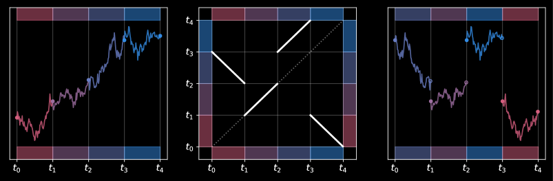
Figure 2: Original path $X$ (left), time permutation $\psi$ defined in (18) with $\xi=(-1,1,1,-1)$ and $\sigma((1,2,3,4))=(3,2,4,1)$ (middle) and transformed path $X\circ\psi$ (right).

Definition 1.

A path functional $F\mathrel{\mathop{\ordinarycolon}}\Lambda\to\operatorname{\mathbb{R}}$ is chronology-invariant if $F(X\circ\psi)=F(X)$ for all $X\in\Lambda_{t}$, $\psi\in\operatorname{\mathfrak{S}}_{t}$, $t\in[0,T]$.

We now see how the chronology invariance relates to occupation functionals. As we are temporarily in a pathwise setting and the quadratic variation is not defined for every càdlàg paths, we employ the standard time occupation measure instead (see Remark 1) and introduce $\tilde{\operatorname{\mathcal{O}}}\mathrel{\mathop{\ordinarycolon}}\Lambda\to\operatorname{\mathcal{M}}$ which maps a path $X\in\Lambda_{t}$ to $\tilde{\operatorname{\mathcal{O}}}_{t}=\tilde{\operatorname{\mathcal{O}}}(X)$. Note in passing that $\tilde{\operatorname{\mathcal{O}}}(X\oplus Y)=\tilde{\operatorname{\mathcal{O}}}(X)+\tilde{\operatorname{\mathcal{O}}}(Y)$ $\forall X,Y\in\Lambda$, so $\tilde{\operatorname{\mathcal{O}}}$ is a homomorphism from $(\Lambda,\oplus)$ to $(\operatorname{\mathcal{M}},+)$.

Next, fix a chronology-invariant functional $F\mathrel{\mathop{\ordinarycolon}}\Lambda_{T}\to\operatorname{\mathbb{R}}$ . Let $I_{n}=[t_{n-1},t_{n})$ as in (18) and introduce the piecewise constant approximation $X^{N}=\sum_{n=1}^{N}\mathds{1}_{I_{n}}X_{t_{n-1}}$ which converges to $X$ pointwise. In particular, we can find $F^{N}\mathrel{\mathop{\ordinarycolon}}\operatorname{\mathbb{R}}^{N}\to\operatorname{\mathbb{R}}$ such that $F(X^{N})=F^{N}(X_{t_{0}},\ldots,X_{t_{N-1}})$. The chronology invariance of $F$ implies that $F^{N}$ must be a symmetric function, hence there exists $f\mathrel{\mathop{\ordinarycolon}}\operatorname{\mathcal{M}}\to\operatorname{\mathbb{R}}$ such that

$$F^{N}(X_{t_{0}},\ldots,X_{t_{N-1}})=f(\tilde{\operatorname{\mathcal{O}}}_{t}^{N}),\qquad\tilde{\operatorname{\mathcal{O}}}_{t}^{N}=\frac{t}{N}\sum_{n=1}^{N}\delta_{X_{t_{n-1}}}.$$ (19)

In mean field games, $F^{N}$ is often called the empirical projection of $f$ [16, I, Chapter 5]. The name has, however, less meaning in the present context. We then have for all $\phi\in\operatorname{\mathcal{C}}_{b}(\operatorname{\mathbb{R}})$ that

$$\int_{\operatorname{\mathbb{R}}}\phi\hskip 0.56905ptd\tilde{\operatorname{\mathcal{O}}}_{t}^{N}=\frac{t}{N}\sum_{n=1}^{N}\phi(X_{t_{n-1}})=\int_{0}^{t}\phi(X_{s}^{N})ds\longrightarrow\int_{0}^{t}\phi(X_{s})ds=\int_{\operatorname{\mathbb{R}}}\phi\hskip 0.56905ptd\tilde{\operatorname{\mathcal{O}}}_{t},$$

by invoking the bounded convergence theorem and occupation time formula (10). This shows the weak convergence of $\tilde{\operatorname{\mathcal{O}}}_{t}^{N}$ to the initial occupation measure $\tilde{\operatorname{\mathcal{O}}}_{t}$. For every bounded linear, chronology-invariant functional $F$, we conclude that $F(X)=\lim_{N\to\infty}f(\tilde{\operatorname{\mathcal{O}}}_{t}^{N})=f(\tilde{\operatorname{\mathcal{O}}}_{t})$, giving a first parallel between chronology invariance and occupation functionals. In fact, we can prove the following general result.

Theorem 2.1.

Let $F\mathrel{\mathop{\ordinarycolon}}\Lambda\to\operatorname{\mathbb{R}}$ be a functional. Then the following are equivalent:

1. $F$ is chronology-invariant.
   

2. There exists a functional $f\mathrel{\mathop{\ordinarycolon}}\operatorname{\mathcal{M}}\to\operatorname{\mathbb{R}}$ such that $F=f\circ\tilde{\operatorname{\mathcal{O}}}.$

Proof.

See Section A.1. ∎

3 Itô’s Calculus

3.1 Occupation Derivative

First, let us motivate the notion of derivative for occupation measures chosen in Definition 3 below. Given $f\mathrel{\mathop{\ordinarycolon}}\operatorname{\mathcal{M}}\to\operatorname{\mathbb{R}}$, we seek an adequate differential operator, say $\delta_{\mu}\mathrel{\mathop{\ordinarycolon}}\operatorname{\mathcal{C}}^{1}(\operatorname{\mathcal{M}})\to\operatorname{\mathcal{C}}(\operatorname{\mathbb{R}})$, with the class $\operatorname{\mathcal{C}}^{1}(\operatorname{\mathcal{M}})$ still to be defined, such that $f(\operatorname{\mathcal{O}}_{t})$ satisfies the chain rule

$$df(\operatorname{\mathcal{O}}_{t})=\delta_{\mu}f(\operatorname{\mathcal{O}}_{t})\cdot d\operatorname{\mathcal{O}}_{t},$$ (20)

with the usual scalar product between functions and measures, namely

$$\phi\cdot\mu\mathrel{\mathop{\ordinarycolon}}=\int_{\operatorname{\mathbb{R}}}\phi(x)\mu(dx),\quad\phi\mathrel{\mathop{\ordinarycolon}}\operatorname{\mathbb{R}}\to\operatorname{\mathbb{R}},\quad\mu\in\operatorname{\mathcal{M}},$$ (21)

whenever the above is well-defined. The dynamics of $\operatorname{\mathcal{O}}$ appearing in (20) still needs to be characterized. Rewriting the occupation measure as $\operatorname{\mathcal{O}}_{t}(A)=\int_{0}^{t}\delta_{X_{u}}(A)d\langle X\rangle_{u}$, where $\delta_{X_{u}}$ is the Dirac mass at the (random) level $X_{u}$, it is then immediate that

$$d\operatorname{\mathcal{O}}_{t}=\delta_{X_{t}}d\langle X\rangle_{t},$$ (22)

and similarly $d\tilde{\operatorname{\mathcal{O}}}_{t}=\delta_{X_{t}}dt$ for the standard time occupation measure $\tilde{\operatorname{\mathcal{O}}}$ seen in (14).

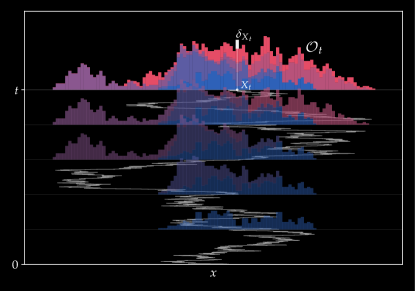
Figure 3: Flow of occupation measures $\operatorname{\mathcal{O}}$ and its dynamics $d\operatorname{\mathcal{O}}_{t}=\delta_{X_{t}}d\langle X\rangle_{t}$.

Expression (22) is intuitive. Within a small time increment, the occupation measure grows in a neighborhood of the current value as the underlying process is continuous. In the limit, $\operatorname{\mathcal{O}}_{t}$ thus increases only at the spot level and proportionally to the stochastic clock of the process; see Fig. 3. Back to the chain rule (20), we therefore conclude that

$$df(\operatorname{\mathcal{O}}_{t})=\delta_{\mu}f(\operatorname{\mathcal{O}}_{t})\cdot d\operatorname{\mathcal{O}}_{t}=\delta_{\mu}f(\operatorname{\mathcal{O}}_{t})\cdot\delta_{X_{t}}d\langle X\rangle_{t}=\delta_{\mu}f(\operatorname{\mathcal{O}}_{t})(X_{t})d\langle X\rangle_{t}.$$ (23)

We would like that (23) at least holds for linear functionals $f(o)=\phi\cdot o$, $\phi\in\operatorname{\mathcal{C}}(\operatorname{\mathbb{R}})$. From the occupation time formula (10), $f(\operatorname{\mathcal{O}}_{t})=\int_{0}^{t}\phi(X_{s})d\langle X\rangle_{s}$. In light of (23), $\delta_{\mu}$ should satisfy

$$\delta_{\mu}(o\mapsto\phi\cdot o)\equiv\phi,\quad\forall\phi\in\operatorname{\mathcal{C}}(\operatorname{\mathbb{R}}).$$ (24)

Hence $\delta_{\mu}$ has to be the usual derivative on space of measures, namely the functional linear derivative commonly used in mean field games and McKean-Vlasov controls [15, 16, 44, 53, 54]. Although typically used for probability measures, we effortlessly extend its definition to arbitrary (finite) measures. In what follows, we endow $\operatorname{\mathcal{M}}$ with the metric $\operatorname{\mathfrak{m}}_{1}$ in Section 2.1, which is equivalent to the total variation distance. We also generalize the scalar product in (21) to signed measures by setting $\phi\cdot\mu=\phi\cdot\mu^{+}-\phi\cdot\mu^{-}$, where $\mu^{+},\mu^{-}$ is respectively the positive and negative part of some signed measure $\mu$.

Definition 2.

A functional $f\mathrel{\mathop{\ordinarycolon}}\operatorname{\mathcal{M}}\to\operatorname{\mathbb{R}}$ is continuously linearly differentiable ($f\in\operatorname{\mathcal{C}}^{1}(\operatorname{\mathcal{M}})$) if there exists $\delta_{\mu}f\mathrel{\mathop{\ordinarycolon}}\operatorname{\mathcal{M}}\to\operatorname{\mathcal{C}}(\operatorname{\mathbb{R}})$, the functional linear derivative of $f$, such that

• The map $\operatorname{\mathcal{M}}\times\operatorname{\mathbb{R}}\ni(\mu,x)\mapsto\delta_{\mu}f(\mu)(x)$ is continuous in the product topology,

• $|\delta_{\mu}f(\mu)(x)|\leq C(1+|x|^{2})$ for some constant $C\in(0,\infty)$, uniformly in $\mu$,

• For all $\mu,\mu^{\prime}\in\operatorname{\mathcal{M}}$ and $\Delta=\mu^{\prime}-\mu$, then

  $$f(\mu^{\prime})-f(\mu)=\int_{0}^{1}\delta_{\mu}f(\mu+\eta\Delta)\cdot\Delta\ d\eta.$$ (25)

We can similarly define the functional linear derivative on $\operatorname{\mathcal{M}}^{\lambda}\subset\operatorname{\mathcal{M}}$ and naturally write $f\in\operatorname{\mathcal{C}}^{1}(\operatorname{\mathcal{M}}^{\lambda})$. In light of (25), we can regard $\delta_{\mu}f(\mu)(x)$ as the Gateaux derivative of $f$ at $\mu$ in the direction $\delta_{x}$, namely $\frac{d}{dh}f(\mu+h\delta_{x})|_{h=0}.$ Hence $\delta_{\mu}$ is akin to a Fréchet derivative; see also Remark 3. In the mean field game literature [16, 15, 53], the functional linear derivative is defined up to an additive constant as it is restricted to probability measures. Indeed, in this context, the signed measure $\Delta=\mu^{\prime}-\mu$ in condition (25) always satisfies $\Delta(\operatorname{\mathbb{R}})=0$. Herein, the total mass of the test measures $\mu,\mu^{\prime}$ may well differ, which pins down $\delta_{\mu}f$ uniquely.

One way to verify that $f\in\operatorname{\mathcal{C}}^{1}(\operatorname{\mathcal{M}})$ (or rather $f\notin\operatorname{\mathcal{C}}^{1}(\operatorname{\mathcal{M}})$; see Example 3) is to compare the left and right functional linear derivative respectively defined as

$$\delta_{\mu}^{-}f(\mu)(x)=\frac{d}{dh}f(\mu+h\operatorname{\mathcal{U}}_{x-h,x})|_{h=0},\quad\delta_{\mu}^{+}f(\mu)(x)=\frac{d}{dh}f(\mu+h\operatorname{\mathcal{U}}_{x,x+h})|_{h=0},$$ (26)

where $\operatorname{\mathcal{U}}_{a,b}$ is the uniform distribution on the interval $[a,b]$, $a<b$.

Remark 3.

Since every element $o\in\operatorname{\mathcal{M}}^{\lambda}$ satisfies $\lVert o\rVert_{2}=\left\lVert\frac{do}{d\lambda}\right\rVert_{L^{2}(\operatorname{\mathbb{R}})}<\infty$, $\delta_{\mu}$ can be regarded as a Fréchet derivative in $L^{2}(\operatorname{\mathbb{R}})$. Given $f\in\operatorname{\mathcal{C}}^{1}(\operatorname{\mathcal{M}}^{\lambda})$, define the lift $F\mathrel{\mathop{\ordinarycolon}}L^{\infty}_{0}(\operatorname{\mathbb{R}})\to\operatorname{\mathbb{R}}$ as $F(\phi)=f(\int_{\cdot}\phi(x)dx)$, hence $f(o)=F\big{(}\frac{do}{d\lambda}\big{)}$. Formally, there exists $\operatorname{\mathfrak{D}}\!F(\phi)\in L^{2}(\operatorname{\mathbb{R}})$, the Fréchet derivative, such that

$$D_{\phi^{\prime}}F(\phi)\mathrel{\mathop{\ordinarycolon}}=\frac{d}{dh}F(\phi+h\phi^{\prime})|_{h=0}=(\operatorname{\mathfrak{D}}\!F(\phi),\phi^{\prime})_{L^{2}(\operatorname{\mathbb{R}})}.$$

On the other hand, if $o,o^{\prime}\in\operatorname{\mathcal{M}}^{\lambda}$ and $\phi=\frac{do}{d\lambda}$, $\phi^{\prime}=\frac{do^{\prime}}{d\lambda}$, we gather from (25) that

$$D_{\phi^{\prime}}F(\phi)=\frac{d}{dh}f(o+ho^{\prime})|_{h=0}=\delta_{\mu}f(o)\cdot o^{\prime}=(\delta_{\mu}f(o),\phi^{\prime})_{L^{2}(\operatorname{\mathbb{R}})}.$$

In conclusion, $\delta_{\mu}f(o)=\operatorname{\mathfrak{D}}\!F\big{(}\frac{do}{d\lambda}\big{)}$ a.e. as expected. See [15, Chapter 1] for a related discussion.

We now introduce a notion of differential tailored to occupation measures.

Definition 3.

The occupation derivative of $f$, denoted by $\partial_{o}f\mathrel{\mathop{\ordinarycolon}}\operatorname{\mathcal{M}}\times\operatorname{\mathbb{R}}\to\operatorname{\mathbb{R}}$, is defined as

$$\partial_{o}f(o,x)=\begin{cases}\delta_{\mu}f(o)(x),\quad&f\in\operatorname{\mathcal{C}}^{1}(\operatorname{\mathcal{M}}),\\[4.0pt] \delta_{\mu}f(o,x)(x),\quad&f\in\operatorname{\mathcal{C}}^{1,0}(\operatorname{\mathcal{M}}\times\operatorname{\mathbb{R}}).\end{cases}$$ (27)

Of course, the occupation derivative can be restricted to $\operatorname{\mathcal{M}}^{\lambda}\times\operatorname{\mathbb{R}}$ or $\operatorname{\mathcal{D}}$. When $f=f(o,x)$, we write $f\in\operatorname{\mathcal{C}}^{1,2}(\operatorname{\mathcal{D}})$ if $\delta_{\mu}f$, $\partial_{x}f$, $\partial_{xx}f$ exist and are jointly continuous. The motivation behind introducing the occupation derivative becomes clear when plugging in the occupied process in (27). Given $f\in\operatorname{\mathcal{C}}^{1}(\operatorname{\mathcal{D}})$, then $\partial_{o}f(\operatorname{\mathcal{O}}_{t},X_{t})$ takes the functional linear derivative $\delta_{\mu}f(\operatorname{\mathcal{O}}_{t},X_{t})(\cdot)$ and evaluates it precisely at $X_{t}$. This is due to the singular dynamics of $\operatorname{\mathcal{O}}$ in (22). This is specific to the occupation measure, whence the terminology for $\partial_{o}$.

As we shall see in Section 3.2.1, the occupation derivative is intrinsically linked to the time derivative in the functional Itô calculus [28]. Similar to the functional derivatives, $\partial_{o}$ and $\partial_{x}$ do not commute. Hence it may happen that the Lie bracket $[\partial_{o},\partial_{x}]f\mathrel{\mathop{\ordinarycolon}}=\partial_{xo}f-\partial_{ox}f$ is nonzero for some $f\mathrel{\mathop{\ordinarycolon}}\operatorname{\mathcal{M}}\to\operatorname{\mathbb{R}}$. A simple example is $f(o,x)=\int_{\operatorname{\mathbb{R}}}yo(dy)$, indeed,

$$\partial_{xo}f(o,x)=1,\quad\partial_{ox}f(o,x)=0,\quad\Longrightarrow[\partial_{o},\partial_{x}]f=1\neq 0.$$

Next, we see how the functional linear derivative and occupation measure interact with each other and finally give a precise meaning of the chain rule (20).

Proposition 3.

Let $X$ be a continuous semimartingale and $f\in\operatorname{\mathcal{C}}^{1}(\operatorname{\mathcal{M}})$. Then for all $s<t$,

$$f(\operatorname{\mathcal{O}}_{t})-f(\operatorname{\mathcal{O}}_{s})=\int_{s}^{t}\partial_{o}f(\operatorname{\mathcal{O}}_{u},X_{u})d\langle X\rangle_{u}=\int_{s}^{t}\delta_{\mu}f(\operatorname{\mathcal{O}}_{u})\cdot d\operatorname{\mathcal{O}}_{u}.$$ (28)

Proof.

It is a byproduct of Itô’s formula for occupied semimartingales; see Theorem 3.1. ∎

For the standard time occupation measure, we similarly have that for $f\in\operatorname{\mathcal{C}}^{1}(\operatorname{\mathcal{M}})$,

$$f(\tilde{\operatorname{\mathcal{O}}}_{t})-f(\tilde{\operatorname{\mathcal{O}}}_{s})=\int_{s}^{t}\partial_{o}f(\tilde{\operatorname{\mathcal{O}}}_{u},X_{u})du=\int_{s}^{t}\delta_{\mu}f(\tilde{\operatorname{\mathcal{O}}}_{u})\cdot d\tilde{\operatorname{\mathcal{O}}}_{u}.$$ (29)

Example 1.

Consider the linear functional $f(o)=\phi\cdot o=\int_{\operatorname{\mathbb{R}}}\phi(x)o(dx)$. In light of the occupation time formula (10), $f(\operatorname{\mathcal{O}}_{t})=\int_{0}^{t}\phi(X_{u})d\langle X\rangle_{u}$. As $\delta_{\mu}f(o)\equiv\phi$ is immediate,

$$f(\operatorname{\mathcal{O}}_{t})-f(\operatorname{\mathcal{O}}_{s})=\int_{0}^{1}\delta_{\mu}f(\operatorname{\mathcal{O}}_{s}+\ \eta\operatorname{\mathcal{O}}_{s,t})\cdot\operatorname{\mathcal{O}}_{s,t}d\eta=\int_{\operatorname{\mathbb{R}}}\phi(x)\operatorname{\mathcal{O}}_{s,t}(dx)=\int_{s}^{t}\phi(X_{u})d\langle X\rangle_{u},$$

which is indeed (28).

Example 2.

Consider the trivial but key example $f(o)=g(o(\operatorname{\mathbb{R}}))$ for some $g\in\operatorname{\mathcal{C}}^{1}([0,T])$. Then $f(\tilde{\operatorname{\mathcal{O}}}_{t})=g(t)$, so $g$ is simply a function of time. Noting that $o(\operatorname{\mathbb{R}})=\mathds{1}\cdot o$ with $\mathds{1}\equiv 1$, we obtain from Example 1 and the chain rule that

$$\partial_{o}f(\tilde{\operatorname{\mathcal{O}}}_{t},X_{t})=\delta_{\mu}f(\tilde{\operatorname{\mathcal{O}}}_{t})(X_{t})=g^{\prime}(\tilde{\operatorname{\mathcal{O}}}_{t}(\operatorname{\mathbb{R}}))\ \underbrace{\delta_{\mu}(\mathds{1}\cdot\tilde{\operatorname{\mathcal{O}}}_{t})(X_{t})}_{=\ 1}=g^{\prime}(t).$$

Applying (29), we therefore recover the fundamental theorem of calculus, namely

$$g(t)-g(s)=f(\tilde{\operatorname{\mathcal{O}}}_{t})-f(\tilde{\operatorname{\mathcal{O}}}_{s})=\int_{s}^{t}\partial_{o}f(\tilde{\operatorname{\mathcal{O}}}_{u},X_{u})du=\int_{s}^{t}g^{\prime}(u)du.$$

We shall see in Example 4 a similar parallel for functionals of the form $f(o,x)=g(o(\operatorname{\mathbb{R}}),x)$.

Example 3.

(Running maximum) Consider the functional

$$M(o)=\sup\Big{\{}x\in\operatorname{\mathbb{R}}\ \mathrel{\mathop{\ordinarycolon}}\ \frac{do}{d\lambda}(x)>0\Big{\}}=\sup\textnormal{supp}(o).$$ (30)

Hence $M(\operatorname{\mathcal{O}}_{t})=\sup_{s\leq t}X_{s}$ is the running maximum of $X$ on $[0,t]$. If $t=0$, we use the convention that $\textnormal{supp}(\operatorname{\mathcal{O}}_{0})=\{X_{0}\}$, i.e., $M(\operatorname{\mathcal{O}}_{0})=X_{0}$. Note that $M\notin\operatorname{\mathcal{C}}^{1}(\operatorname{\mathcal{M}}^{\lambda})$ as the left and right functional linear derivatives (26) differ at the maximum $x=M(o)$. Indeed, it is easy to see that $\delta_{\mu}^{+}M(o)(x)|_{x=M(o)}=1$ while $\delta_{\mu}^{-}M(o)(x)|_{x=M(o)}=0$ as the direction $\operatorname{\mathcal{U}}_{x-h,x}$ in (26) does not alter the rightmost end of $\text{supp}(o)$ for all $x\leq M(o)$. We thus need a mollified version of $M$ to apply Proposition 3. Given $o\in\operatorname{\mathcal{M}}^{\lambda}$, $o(\operatorname{\mathbb{R}})>0$, consider the smooth functional (akin to the log-sum-exp function in machine learning),

$$M^{\varepsilon}(o)=\varepsilon\log\mathop{\,\,\hbox to0.0pt{--\hss}\int}\nolimits_{\operatorname{\mathbb{R}}}e^{x/\varepsilon}o(dx).$$ (31)

where we recall that $\mathop{\,\,\hbox to0.0pt{--\hss}\int}\nolimits_{A}fdo=\frac{1}{o(A)}\int_{A}fdo$. If $o(\operatorname{\mathbb{R}})=0$ and $\text{supp}(o)=\{x\}$ (e.g., $o=\operatorname{\mathcal{O}}_{0}$), we set $M^{\varepsilon}(o)=x$. Next, define $\psi(x)\mathrel{\mathop{\ordinarycolon}}=e^{x-M(o)}$ and decompose $M^{\varepsilon}$ as

$$M^{\varepsilon}(o)=\varepsilon\log\mathop{\,\,\hbox to0.0pt{--\hss}\int}\nolimits_{\operatorname{\mathbb{R}}}(e^{M(o)}\psi)^{1/\varepsilon}do=M(o)+\log\ \lVert\psi\rVert_{L^{1/\varepsilon}(o)}-\varepsilon\log o(\operatorname{\mathbb{R}}).$$

As $|\psi|\leq 1$ in the compact $\text{supp}(o)$, then $\psi\in L^{p}(o)\ \forall p\in[1,\infty]$. This implies that $\lim_{\varepsilon\downarrow 0}\ \lVert\psi\rVert_{L^{1/\varepsilon}(o)}=\lVert\psi\rVert_{L^{\infty}(o)}=\psi(M(o))=1$ and thus $M^{\varepsilon}\to M$ pointwise. Let us compute the occupation derivative of $M^{\varepsilon}$. Thanks to Examples 1, 2 and the chain rule, this gives

$$\partial_{o}M^{\varepsilon}(o,x)=\delta_{\mu}M^{\varepsilon}(o)(x)=\frac{\varepsilon\ e^{x/\varepsilon}}{\int_{\operatorname{\mathbb{R}}}e^{y/\varepsilon}o(dy)}-\frac{\varepsilon}{o(\operatorname{\mathbb{R}})}=\frac{\varepsilon}{o(\operatorname{\mathbb{R}})}\left(e^{[x-M^{\varepsilon}(o)]/{\varepsilon}}-1\right).$$ (32)

Hence $M^{\varepsilon}\in\operatorname{\mathcal{C}}^{1}(\operatorname{\mathcal{M}}^{\lambda})$ and Proposition 3 yields $M^{\varepsilon}(\operatorname{\mathcal{O}}_{t})=X_{0}+\int_{0}^{t}\delta_{\mu}M^{\varepsilon}(\operatorname{\mathcal{O}}_{s})\cdot d\operatorname{\mathcal{O}}_{s}$. We now study the behavior of $\delta_{\mu}M^{\varepsilon}(o)$ as $\varepsilon\to 0$. If $x<M(o)$, then $x-M^{\varepsilon}(o)<0$ for sufficiently small $\varepsilon$ and thus $\delta_{\mu}M^{\varepsilon}(o)\to 0$ according to (32). If $x=M(o)$ and $\text{supp}(o)\neq\{M(o)\}$, then

$$\left(\varepsilon\ e^{[M(o)-M^{\varepsilon}(o)]/{\varepsilon}}\right)^{-1}=\frac{1}{\varepsilon o(\operatorname{\mathbb{R}})}\lVert\psi\rVert_{L^{1/\varepsilon}(o)}^{1/\varepsilon}=\mathop{\,\,\hbox to0.0pt{--\hss}\int}\nolimits_{\operatorname{\mathbb{R}}}\frac{1}{\varepsilon}e^{(x-M(o))/\varepsilon}o(dx)\to 0.$$

Hence $\partial_{o}M^{\varepsilon}(o,M(o))\to\infty$ in light of (32), so $\delta_{\mu}M(o)$ converges formally to the Dirac mass at $M(o)$. Writing $M_{t}\mathrel{\mathop{\ordinarycolon}}=M(\operatorname{\mathcal{O}}_{t})$ for the running maximum process, we obtain

$$M_{t}-X_{0}=\lim_{\varepsilon\downarrow 0}M^{\varepsilon}(\operatorname{\mathcal{O}}_{t})-X_{0}=\int_{0}^{t}\delta_{M(\operatorname{\mathcal{O}}_{s})}\cdot d\operatorname{\mathcal{O}}_{s}=\int_{0}^{t}\delta_{M_{s}}(X_{s})d\langle X\rangle_{s}=L_{t}^{0}(M-X),$$

where $L^{0}(M-X)$ is the local time at zero of the reflected process $M_{t}-X_{t}=\sup_{s\leq t}X_{s}-X_{t}$. We thus recover the equality $M_{t}=X_{0}+L^{0}_{t}(M-X)\ \operatorname{\mathbb{Q}}-a.s.$ established by Dupire [28, Example 2], generalizing Lévy’s distributional result.

3.2 Itô’s Formula

We now state Itô’s formula for continuous occupied semimartingales in one space dimension. For the multi-dimensional case, see Remark 4.

Theorem 3.1.

(Itô’s formula) Let $X$ be a continuous semimartingale and $\operatorname{\mathcal{O}}$ its flow of occupation measures. If $f\in\operatorname{\mathcal{C}}^{1,2}(\operatorname{\mathcal{D}})$, then

$$f(\operatorname{\mathcal{O}}_{t},X_{t})-f(\operatorname{\mathcal{O}}_{s},X_{s}) =\int_{s}^{t}\Big{(}\partial_{o}+\frac{1}{2}\partial_{xx}\Big{)}f(\operatorname{\mathcal{O}}_{u},X_{u})d\langle X\rangle_{u}+\int_{s}^{t}\partial_{x}f(\operatorname{\mathcal{O}}_{u},X_{u})dX_{u}.$$ (33)

In terms of the functional linear derivative and dynamics of $\operatorname{\mathcal{O}}$, we can also write

$$\int_{s}^{t}\Big{(}\partial_{o}+\frac{1}{2}\partial_{xx}\Big{)}f(\operatorname{\mathcal{O}}_{u},X_{u})d\langle X\rangle_{u} =\int_{s}^{t}\Big{(}\delta_{\mu}f(\operatorname{\mathcal{O}}_{u},X_{u})+\frac{1}{2}\partial_{xx}f(\operatorname{\mathcal{O}}_{u},\cdot)\Big{)}\cdot d\operatorname{\mathcal{O}}_{u}.$$ (34)

Proof.

See Section A.2. ∎

Remark 4.

If $X$ is a semimartingale living in $\operatorname{\mathbb{R}}^{d}$, $d\geq 2$, then the occupation measure $\operatorname{\mathcal{O}}$ is a random element of $\operatorname{\mathcal{M}}_{d}\mathrel{\mathop{\ordinarycolon}}=\{o\mathrel{\mathop{\ordinarycolon}}\operatorname{\mathcal{B}}(\operatorname{\mathbb{R}}^{d})\to[0,\infty)\mathrel{\mathop{\ordinarycolon}}\text{Radon measure}\}$. Theorem 3.1 is easily generalized. For example, if $f\in\operatorname{\mathcal{C}}^{1,2}(\operatorname{\mathcal{M}}_{d}\times\operatorname{\mathbb{R}}^{d})$ and $X$ is Brownian motion in $\operatorname{\mathbb{R}}^{d},$ then

$$f(\operatorname{\mathcal{O}}_{t},X_{t})-f(\operatorname{\mathcal{O}}_{s},X_{s}) =\int_{s}^{t}\Big{(}\partial_{o}+\frac{1}{2}\Delta\Big{)}f(\operatorname{\mathcal{O}}_{u},X_{u})du+\int_{s}^{t}\nabla f(\operatorname{\mathcal{O}}_{u},X_{u})^{\top}dX_{u},$$ (35)

where $\nabla,\ \Delta$ is the gradient and Laplace operator, respectively. Importantly, $\operatorname{\mathcal{O}}$ is still one single entity, akin to the time variable.

Remark 5.

If $\operatorname{\mathcal{O}}$ is replaced by the standard time occupation measure in Theorem 3.1, then we can easily show for $f\in\operatorname{\mathcal{C}}^{1,2}(\operatorname{\mathcal{M}}\times\operatorname{\mathbb{R}})$ that $f(\tilde{\operatorname{\mathcal{O}}}_{t},X_{t})$ has dynamics (in differential form),

$$df(\tilde{\operatorname{\mathcal{O}}}_{t},X_{t})=\partial_{o}f(\tilde{\operatorname{\mathcal{O}}}_{t},X_{t})dt+\partial_{x}f(\tilde{\operatorname{\mathcal{O}}}_{t},X_{t})dX_{t}+\frac{1}{2}\partial_{xx}f(\tilde{\operatorname{\mathcal{O}}}_{t},X_{t})d\langle X\rangle_{t}.$$ (36)

Example 4.

Let $f(o,x)=g(o(\operatorname{\mathbb{R}}),x)$ for some $g\in\operatorname{\mathcal{C}}^{1,2}([0,T]\times\operatorname{\mathbb{R}})$. Then $f(\tilde{\operatorname{\mathcal{O}}}_{t},X_{t})=g(t,X_{t})$. Similarly to Example 2, we have $\partial_{o}f=\partial_{t}g$. As $\partial_{x}g=\partial_{x}f$, $\partial_{xx}g=\partial_{xx}f$, we therefore recover from (36) the classical Itô’s formula, that is

$$dg(t,X_{t}) =\partial_{t}g(t,X_{t})dt+\partial_{x}g(t,X_{t})dX_{t}+\frac{1}{2}\partial_{xx}g(t,X_{t})d\langle X\rangle_{t}.$$

3.2.1 Connection with the Functional Itô Calculus

We first outline the functional Itô formula proved by Dupire [28]. Let $\Lambda_{t},\Lambda$ as in Section 2.3 and endow $\Lambda$ with the measure $\operatorname{\mathbb{Q}}$. If $F\mathrel{\mathop{\ordinarycolon}}\Lambda\to\operatorname{\mathbb{R}}$ is a functional with continuous temporal and spatial derivatives $\Delta_{t}F,\ \Delta_{x}F,\ \Delta_{xx}F$ defined in [28], then

$$dF(X)=\Delta_{t}F(X)dt+\Delta_{x}F(X)dX_{t}+\frac{1}{2}\Delta_{xx}F(X)d\langle X\rangle_{t},$$ (37)

for $\operatorname{\mathbb{Q}}-$almost every $X\in\Lambda_{t}$. To connect (37) with Theorem 3.1, fix $f\in\operatorname{\mathcal{C}}^{1,2}(\operatorname{\mathcal{M}}\times\operatorname{\mathbb{R}})$ and define the functional $F(X)=f(\tilde{\operatorname{\mathcal{O}}}(X),X_{t})=f(\tilde{\operatorname{\mathcal{O}}}_{t},X_{t})$ where, as in Section 2.3, $\tilde{\operatorname{\mathcal{O}}}\mathrel{\mathop{\ordinarycolon}}\Lambda\to\operatorname{\mathcal{M}}$ maps a path to its standard time occupation measure. We now aim at rewriting and fix $X\in\Lambda_{t}$ in what follows. Starting with the functional time derivative, we have

$$\Delta_{t}F(X)\mathrel{\mathop{\ordinarycolon}}=\lim_{h\downarrow 0}\ \frac{F(X_{\oplus h})-F(X)}{h}=\lim_{h\downarrow 0}\ \frac{f(\tilde{\operatorname{\mathcal{O}}}(X_{\oplus h}),X_{t})-f(\tilde{\operatorname{\mathcal{O}}}_{t},X_{t})}{h},$$ (38)

with the extended path $X_{\oplus h}=(X_{u\wedge t})_{u\leq t+h}$. First, $(\tilde{\operatorname{\mathcal{O}}}(X_{\oplus h})-\tilde{\operatorname{\mathcal{O}}}_{t})(A)=h\mathds{1}_{A}(X_{t})$, $A\in\operatorname{\mathcal{B}}(\operatorname{\mathbb{R}})$, hence $\frac{1}{h}[\tilde{\operatorname{\mathcal{O}}}(X_{\oplus h})-\tilde{\operatorname{\mathcal{O}}}_{t}]=\delta_{X_{t}}$ for all $h\geq 0$. We then invoke condition (25) satisfied by the functional linear derivative to obtain

$$\lim_{h\downarrow 0}\frac{f(\tilde{\operatorname{\mathcal{O}}}(X_{\oplus h}),X_{t})-f(\tilde{\operatorname{\mathcal{O}}}_{t},X_{t})}{h}=\lim_{h\downarrow 0}\int_{0}^{1}\delta_{\mu}f(\tilde{\operatorname{\mathcal{O}}}_{t}+\eta h\delta_{X_{t}},X_{t})\cdot\delta_{X_{t}}d\eta=\delta_{\mu}f(\tilde{\operatorname{\mathcal{O}}}_{t},X_{t})(X_{t}).$$

We therefore obtain the following connection between functional time derivative and the occupation derivative,

$$\Delta_{t}F(X)=\partial_{o}f(\tilde{\operatorname{\mathcal{O}}}_{t},X_{t}),\quad X\in\Lambda_{t}.$$ (39)

Equality (39) further confirms that the (standard time) occupation measure plays the same role as $t$. Moreover, $\Delta_{x}F=\partial_{x}f$ and $\Delta_{xx}F=\partial_{xx}f$ as a vertical bump of $X$ at $t$ does not affect the Lebesgue integrals $\int_{0}^{t}\mathds{1}_{\cdot}(X_{s})ds$ and the measure-valued functional $\tilde{\operatorname{\mathcal{O}}}$ is thus unchanged. All in all, we obtain that

$$df(\tilde{\operatorname{\mathcal{O}}}_{t},X_{t}) =dF(X)$$

$$=\Delta_{t}F(X)dt+\Delta_{x}F(X)dX_{t}+\frac{1}{2}\Delta_{xx}F(X)d\langle X\rangle_{t}$$

$$=\partial_{o}f(\tilde{\operatorname{\mathcal{O}}}_{t},X_{t})dt+\partial_{x}f(\tilde{\operatorname{\mathcal{O}}}_{t},X_{t})dX_{t}+\frac{1}{2}\partial_{xx}f(\tilde{\operatorname{\mathcal{O}}}_{t},X_{t})d\langle X\rangle_{t},$$

which is (36).

Figure 4: Functional time derivative $\Delta_{t}$ (left) and occupation time derivative $\partial_{o}$ (right) linked in display (39). Note that the whole path has to be retained to compute $\Delta_{t}$, while $\partial_{o}$ depends solely on the standard time occupation measure $\tilde{\operatorname{\mathcal{O}}}_{t}$ and the spot value $X_{t}$.

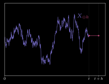
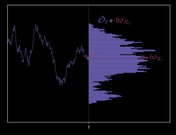
Remark 6.

The above connection would not work if $\tilde{\operatorname{\mathcal{O}}}$ is replaced by $\operatorname{\mathcal{O}}$. Indeed, suppose we were able to define $\operatorname{\mathcal{O}}(X)(A)=\int_{0}^{t}\mathds{1}_{A}(X_{s})d\langle X\rangle_{s}$ pathwise and set $F(X)=f(\operatorname{\mathcal{O}}(X),X_{t})$, $X\in\Lambda_{t}$. As the extended path $X_{\oplus h}$ has zero quadratic variation in the interval $[t,t+h]$, then $\operatorname{\mathcal{O}}(X_{\oplus h})=\operatorname{\mathcal{O}}(X)$ and in turn $\Delta_{t}F(X)=0$. However, comparing (33) and (37), we must have that

$$\Delta_{t}F(X)dt=\partial_{o}f(\operatorname{\mathcal{O}}_{t},X_{t})d\langle X\rangle_{t},\quad\operatorname{\mathbb{Q}}-a.s.$$ (40)

This confirms that establishing a pathwise calculus for the occupation measure $\operatorname{\mathcal{O}}$ would typically fail.

3.2.2 Connection with the Malliavin Calculus

The goal of this section is to regard ”terminal” functionals $f(\operatorname{\mathcal{O}}_{T})$ through the lens of Malliavin calculus (see, e.g., [26]). Suppose that $\operatorname{\mathbb{Q}}$ is the Wiener measure so that the canonical process is Brownian motion. As $\langle X\rangle_{t}=t$ $\operatorname{\mathbb{Q}}-a.s.$, the flows $\operatorname{\mathcal{O}}$ and $\tilde{\operatorname{\mathcal{O}}}$ coincide almost surely so we can define the measure-valued functional $\operatorname{\mathcal{O}}(X)(A)=\int_{0}^{T}\mathds{1}_{A}(X_{t})dt$, $X\in\Lambda_{T}$. We can then prove the following result connection the Malliavin derivative with the mixed derivative $\partial_{xo}$.

Proposition 4.

Let $f\in\operatorname{\mathcal{C}}^{1}(\operatorname{\mathcal{M}})$ such that $x\mapsto\partial_{o}f(o,x)$ is differentiable for every $o\in\operatorname{\mathcal{M}}^{\lambda}$ and $F(X)\mathrel{\mathop{\ordinarycolon}}=f(\operatorname{\mathcal{O}}(X))=f(\operatorname{\mathcal{O}}_{T})$, $X\in\Lambda_{T}$, is Malliavin differentiable. Then, the Malliavin derivative of $F(X)$ admits the expression

$$D_{t}F(X)\mathrel{\mathop{\ordinarycolon}}=\frac{d}{dh}F(X+h\mathds{1}_{[t,T]})\Big{|}_{h=0}=\int_{t}^{T}\partial_{xo}f(\operatorname{\mathcal{O}}_{T},X_{u})du,\quad\operatorname{\mathbb{Q}}-a.s.$$ (41)

Proof.

See Section A.3. ∎

Remark 7.

Observe from (41) that $\operatorname{\mathfrak{D}}\!F(X)\mathrel{\mathop{\ordinarycolon}}=-\partial_{t}D_{\cdot}f(\operatorname{\mathcal{O}}_{T})=\partial_{xo}f(\operatorname{\mathcal{O}}_{T},X_{\cdot})\in L^{2}([0,T])$ is precisely the Fréchet derivative of $F$, i.e.

$$\frac{d}{dh}F(X+Y)\Big{|}_{h=0}=(\operatorname{\mathfrak{D}}\!F(X),Y)_{L^{2}([0,T])}=\int_{0}^{T}\partial_{xo}f(\operatorname{\mathcal{O}}_{T},X_{t})Y_{t}dt\quad\forall\ Y\in\Lambda_{T}.$$

Regarding $F(X)=f\circ\operatorname{\mathcal{O}}$ as the lift of the occupation functional $f\mathrel{\mathop{\ordinarycolon}}\operatorname{\mathcal{M}}\to\operatorname{\mathbb{R}}$, then the identity $\operatorname{\mathfrak{D}}\!F(X)=\partial_{x}\delta_{\mu}f(\operatorname{\mathcal{O}}_{T})(X_{\cdot})$ is similar in spirit to the link between $\delta_{\mu}$ and the Lions derivative in mean field games [15, 16, 44].

3.3 Feynman-Kac’s Formula for the Backward Heat Equation

We first prove a Feynman-Kac theorem for occupied Brownian motion. A more general result will be given in in Section 3.4. Write $\varphi\in\operatorname{\mathcal{C}}^{2}_{2}(\operatorname{\mathcal{D}})$ if $\varphi\in\operatorname{\mathcal{C}}^{2,2}(\operatorname{\mathcal{D}})$ and $(x,y)\mapsto\delta_{\mu}\varphi(o,x)(y)$, $(y,y^{\prime})\mapsto\delta_{\mu\mu}\varphi(o,x)(y,y^{\prime})$ are twice continuously differentiable with bounded derivatives.

Theorem 3.2.

(Feynman-Kac) Let $\varphi\mathrel{\mathop{\ordinarycolon}}\operatorname{\mathcal{D}}\to\operatorname{\mathbb{R}}$ such that $\varphi(\operatorname{\mathcal{O}}_{T},X_{T})\in L^{1}(\operatorname{\mathbb{Q}})$ and consider the backward heat equation,

$$\Big{(}\partial_{o}+\frac{1}{2}\partial_{xx}\Big{)}v=0, \operatorname{\mathcal{D}}_{T}\mathrel{\mathop{\ordinarycolon}}=\{(o,x)\in\operatorname{\mathcal{D}}\mathrel{\mathop{\ordinarycolon}}o(\operatorname{\mathbb{R}})<T\}$$ on , (42a)

$$v=\varphi, \partial\!\operatorname{\mathcal{D}}_{T}\mathrel{\mathop{\ordinarycolon}}=\{(o,x)\in\operatorname{\mathcal{D}}\mathrel{\mathop{\ordinarycolon}}o(\operatorname{\mathbb{R}})=T\}$$ on . (42b)

If $v\in\operatorname{\mathcal{C}}^{1,2}(\operatorname{\mathcal{D}})$ is a classical solution of (42a)$-$(42b), then it admits the representation

$$v(o,x)=\operatorname{\mathbb{E}}_{o,x}^{\operatorname{\mathbb{Q}}}[\varphi(\operatorname{\mathcal{O}}_{T},X_{T})]\mathrel{\mathop{\ordinarycolon}}=\operatorname{\mathbb{E}}^{\operatorname{\mathbb{Q}}}[\varphi(o+\operatorname{\mathcal{O}}_{T-t}^{x},x+X_{T-t})],\quad o(\operatorname{\mathbb{R}})=t,$$ (43)

where $\operatorname{\mathcal{O}}_{s}^{x}(A)=\operatorname{\mathcal{O}}_{s}(A-x)$. Conversely, if $\varphi\in\operatorname{\mathcal{C}}^{2}_{2}(\operatorname{\mathcal{D}})$, then $v$ in (43) belongs to $\operatorname{\mathcal{C}}^{2}_{2}(\operatorname{\mathcal{D}})$ as well and is the unique classical solution of (42a)$-$(42b).

Proof.

See Section A.4. ∎

We finally discuss several examples where $\varphi$ has little regularity while the value functional is still smooth. As we shall see, this is in contrast with other path-dependent calculi where the associated value functional typically fails to be even continuous.

Example 5.

(Local time at zero) Let $X$ be Brownian motion and $\varphi(o,x)=\frac{do}{d\lambda}(0)$, irrespective of $x$. Hence $\varphi(\operatorname{\mathcal{O}}_{T},X_{T})=L_{T}^{0}$ is the local time at $0$. If $(o,x)\in\partial\operatorname{\mathcal{D}}_{t}$, a simple calculation shows that

$$v(o,x) =\operatorname{\mathbb{E}}^{\operatorname{\mathbb{Q}}}_{o,x}[L_{T}^{0}]=\operatorname{\mathbb{E}}^{\operatorname{\mathbb{Q}}}_{o,x}\left[L_{t}^{0}+L_{t,T}^{0}\right]=\frac{do}{d\lambda}(0)+\operatorname{\mathbb{E}}^{\operatorname{\mathbb{Q}}}_{x}[L_{T-t}^{0}]=\frac{do}{d\lambda}(0)+\operatorname{\mathbb{E}}^{\operatorname{\mathbb{Q}}}[L_{T-t}^{|x|}].$$

The first term in the last equality is linear in $o$ and Lipschitz continuous with respect to the metric $\operatorname{\mathfrak{m}}_{\infty}$ seen in Section 2.1. Moreover, the second term is continuous in $x$ and even piecewise smooth on $\operatorname{\mathbb{R}}\setminus\{0\}$ for all $t<T$. In the pathwise setting as in Section 3.2.1, we note that the functional

$$V(X)=\operatorname{\mathbb{E}}^{\operatorname{\mathbb{Q}}}[L_{T}^{0}\ |\ X]=L^{0}(X)+\operatorname{\mathbb{E}}^{\operatorname{\mathbb{Q}}}\big{[}L_{T-t}^{|x|}\big{]}|_{x=X_{t}},\quad X\in\Lambda_{t},$$ (44)

is not continuous in the input path (with respect to the supremum norm), regardless of the definition of $L^{0}\mathrel{\mathop{\ordinarycolon}}\Lambda\to\operatorname{\mathbb{R}}$. First, one may set $L^{0}(X)=\lim_{\varepsilon\to 0}\frac{1}{2\varepsilon}\int_{0}^{t}\mathds{1}_{B_{\varepsilon}}(X_{s})ds$ as the occupation measures $\operatorname{\mathcal{O}},\tilde{\operatorname{\mathcal{O}}}$ almost surely coincide under the Wiener measure. However, if $(X^{N})$ is a sequence of piecewise linear paths that converges to $X$ (e.g. using Schauder’s theorem) it may happen that $L^{0}(X^{N})=\infty$ as the occupation measure of $X^{N}$ is not absolutely continuous with respect to $\lambda$. Another possibility is $L^{0}(X)\mathrel{\mathop{\ordinarycolon}}=\lim_{\varepsilon\to 0}\frac{1}{2\varepsilon}\int_{0}^{t}\mathds{1}_{B_{\varepsilon}}(X_{s})d\langle X\rangle_{s}$ when $\langle X\rangle$ is well-defined. But for the sequence $(X^{N})$ above, we have $L^{0}(X^{N})=0$ leading again to the discontinuity of $L^{0}$ with respect to $X$. Finally, we could derive the local time at zero (or any other level) from Tanaka’s formula [51, Chapter VI]. However, the expression would involve stochastic integrals which are infamously discontinuous with respect to the input path. This representation is thus subject to the same fate as the previous ones.

Example 6.

(Spot Local time) Let $\varphi(o,x)=\frac{do}{d\lambda}(x)$, that is $\varphi(\operatorname{\mathcal{O}}_{t},X_{t})=L_{t}^{X_{t}}$. Then $\varphi$ is continuous in $x$ (as $X$ is a continuous martingale) and in $o$ with respect to $\operatorname{\mathfrak{m}}_{\infty}$. However, $\varphi$ is not differentiable in $x$. For every $(o,x)\in\partial\operatorname{\mathcal{D}}_{t}$, $t<T$, we first write the value function as

$$v(o,x)=\operatorname{\mathbb{E}}^{\operatorname{\mathbb{Q}}}_{o,x}[L_{T}^{X_{T}}]=\int_{\operatorname{\mathbb{R}}}\frac{do}{d\lambda}(y)\phi_{T-t}(y-x)dy+\operatorname{\mathbb{E}}^{\operatorname{\mathbb{Q}}}\big{[}L_{T-t}^{X_{T-t}}\big{]},$$

where $\phi_{s}$ is the density of $\operatorname{\mathcal{N}}(0,s).$ From $\frac{do}{d\lambda}(y)dy=o(dy)$ and Proposition 5 below, we obtain

$$v(o,x)=\int_{\operatorname{\mathbb{R}}}\phi_{T-t}(y-x)o(dy)+\operatorname{\mathbb{E}}^{\operatorname{\mathbb{Q}}}[L_{T-t}^{0}].$$ (45)

The first term on the right side of (45) is linear in $o$ and smooth in $x$ for all $t<T$. As the second term is independent of $(o,x)$, $v$ is therefore smooth. On the other hand, the path functional $V(X)=\operatorname{\mathbb{E}}^{\operatorname{\mathbb{Q}}}[L_{T}^{X_{T}}\ |\ X]$ is discontinuous with respect to $X$ as in Example 5.

3.4 Occupied SDEs and Dirichlet Problems

Let $b,\sigma\in\operatorname{\mathcal{C}}(\operatorname{\mathcal{D}})$ and consider the occupied stochastic differential equation (OSDE),

$$d\operatorname{\mathcal{O}}_{t}=\delta_{X_{t}}d\langle X\rangle_{t}, \operatorname{\mathcal{O}}_{0}\in\operatorname{\mathcal{M}}$$ , (46a)

$$dX_{t}=b(\operatorname{\mathcal{O}}_{t},X_{t})dt+\sigma(\operatorname{\mathcal{O}}_{t},X_{t})dW_{t},\; X_{0}\in\text{supp}(\operatorname{\mathcal{O}}_{0}).$$ (46b)

Note that (46a) can be equivalently written as $d\operatorname{\mathcal{O}}_{t}=\delta_{X_{t}}\sigma(\operatorname{\mathcal{O}}_{t},X_{t})^{2}dt$. We refer to Section 5.4 for the numerical integration of (46a)$-$(46b). Assuming the usual Lipschitz and linear growth condition on $b,\sigma$ (with respect to the $\operatorname{\mathfrak{m}}_{1}$ metric for the occupation measure), it is expected that (46b) admits a unique strong solution. A thorough analysis of this class of SDEs is nevertheless postponed to another study. Occupied SDEs share similarities with the fashionable McKean-Vlasov SDEs [16, 44] (here autonomous for simplicity),

$$\mu_{t}=\ \text{Law}_{\operatorname{\mathbb{Q}}}(X_{t}), \mu_{0}\in\operatorname{\mathcal{M}},\ \mu_{0}(\operatorname{\mathbb{R}})=1,$$

$$dX_{t}=b(\mu_{t},X_{t})dt+\sigma(\mu_{t},X_{t})dW_{t},\; X_{0}\sim\mu_{0}.$$

We note that both (46a)$-$(46b) and the McKean-Vlasov system must solve a fixed point equation, that is $\operatorname{\mathcal{O}}_{t}$ (resp. $\mu_{t}$) must be precisely the flow of occupation measures (resp. marginal laws) of $X$. Although the structure looks similar when considering $\operatorname{\mathcal{O}}_{t}$ or $\text{Law}(X_{t})$, their actual meanings are obviously poles apart. While Itô’s formula for McKean-Vlasov processes may be quite involved as the marginal laws may interact with martingale part [35, 53], the analogue for OSDEs remains simple due to the singular dynamics of $\operatorname{\mathcal{O}}$.

Theorem 3.3.

(Itô’s formula for OSDEs) Let $(\operatorname{\mathcal{O}},X)$ be a strong solution of the OSDE (46a)$-$(46b) with drift diffusion $b,\sigma$, respectively. If $f\in\operatorname{\mathcal{C}}^{1,2}(\operatorname{\mathcal{D}})$, then

$$f(\operatorname{\mathcal{O}}_{t},X_{t})-f(\operatorname{\mathcal{O}}_{s},X_{s}) =\int_{s}^{t}\operatorname{\mathcal{L}}f(\operatorname{\mathcal{O}}_{u},X_{u})du+\int_{s}^{t}\sigma(\operatorname{\mathcal{O}}_{u},X_{u})\partial_{x}f(\operatorname{\mathcal{O}}_{u},X_{u})dW_{u},$$ (48)

$$\operatorname{\mathcal{L}} =\sigma^{2}\partial_{o}+b\ \partial_{x}+\frac{\sigma^{2}}{2}\partial_{xx}.$$ (49)

Proof.

This is a direct consequence of Theorem 3.1. ∎

Next, we aim to extend Feynman-Kac’s representation seen so far for Brownian motion (Theorem 3.2). If $(\operatorname{\mathcal{O}}^{o,x},X^{o,x})$ denotes the solution of the OSDE (46a)$-$(46b) given $(\operatorname{\mathcal{O}}_{t},X_{t})=(o,x)$, it is tempting to define $v(o,x)=\operatorname{\mathbb{E}}^{\operatorname{\mathbb{Q}}}[\varphi(\operatorname{\mathcal{O}}_{T}^{o,x},X_{T}^{o,x})]$ as in (43). Thanks to the previous Itô’s formula and the martingality of $v(\operatorname{\mathcal{O}},X)$, we indeed obtain that $v$ satisfies $\operatorname{\mathcal{L}}v=0$ with $\operatorname{\mathcal{L}}$ given in (49). There is however an irremediable twist: unlike Brownian motion or any continuous Gaussian martingale where $\operatorname{\mathcal{O}}_{T}(\operatorname{\mathbb{R}})=\langle X\rangle_{T}$ is deterministic, the total mass may well be path-dependent (take for instance, $b\equiv 0$ and $\sigma(o,x)=x$). Hence the terminal condition is in general misspecified!

A remedy is to replace the horizon $T$ by the random date at which the total mass $\operatorname{\mathcal{O}}(\operatorname{\mathbb{R}})$ first exceeds a threshold, say $\Theta>0$. With this new interpretation, the terminal date becomes stochastic and corresponds to the exit time $\tau_{\Theta}$ of $\operatorname{\mathcal{O}}$ from the open $\operatorname{\mathfrak{m}}_{1}-$ball $\operatorname{\mathcal{M}}_{\Theta}\mathrel{\mathop{\ordinarycolon}}=\{o\in\operatorname{\mathcal{M}}\mathrel{\mathop{\ordinarycolon}}\lVert o\rVert_{1}<\Theta\}=\{o\in\operatorname{\mathcal{M}}\mathrel{\mathop{\ordinarycolon}}o(\operatorname{\mathbb{R}})<\Theta\}$, namely

$$\tau_{\Theta}=\inf\{t\geq 0\ \mathrel{\mathop{\ordinarycolon}}\operatorname{\mathcal{O}}_{t}(\operatorname{\mathbb{R}})\notin\operatorname{\mathcal{M}}_{\Theta}\}=\inf\{t\geq 0\ \mathrel{\mathop{\ordinarycolon}}\langle X\rangle_{t}\geq\Theta\}.$$ (50)

This is precisely the logic behind the DDS transformation seen in Remark 2. In finance, contracts where the maturity is dictated by the quadratic variation of the (log) asset price are termed timer or Dirichlet options; see Section 5.2 below. We now state a Feynman-Kac’s theorem for OSDEs. Its proof is almost identical to the first part in Theorem 3.2.

Theorem 3.4.

(Feynman-Kac) Let $\varphi\mathrel{\mathop{\ordinarycolon}}\operatorname{\mathcal{D}}\to\operatorname{\mathbb{R}}$ such that $\varphi(\operatorname{\mathcal{O}}_{T},X_{T})\in L^{1}(\operatorname{\mathbb{Q}})$ and consider the Dirichlet problem

$$\operatorname{\mathcal{L}}v=0, \operatorname{\mathcal{D}}_{\Theta}=\{(o,x)\in\operatorname{\mathcal{D}}\ \mathrel{\mathop{\ordinarycolon}}\ o(\operatorname{\mathbb{R}})<\Theta\},$$ on (51a)

$$v=\varphi, \partial\!\operatorname{\mathcal{D}}_{\Theta}=\{(o,x)\in\operatorname{\mathcal{D}}\ \mathrel{\mathop{\ordinarycolon}}\ o(\operatorname{\mathbb{R}})=\Theta\},$$ on (51b)

with $\varphi\mathrel{\mathop{\ordinarycolon}}\operatorname{\mathcal{D}}\to\operatorname{\mathbb{R}}$, $\operatorname{\mathcal{L}}$ given by in (49). Let $\tau_{\Theta}$ be the exit time of $\operatorname{\mathcal{M}}_{\Theta}$ as in (50) and suppose that $\operatorname{\mathbb{E}}^{\operatorname{\mathbb{Q}}}[\tau_{\Theta}]<\infty$. If $(\operatorname{\mathcal{O}},X)$ is a strong solution of (46a)$-$(46b) and (51a)$-$(51b) has a classical solution $v\in\operatorname{\mathcal{C}}^{1,2}(\operatorname{\mathcal{D}})$, then

$$v(o,x)=\operatorname{\mathbb{E}}^{\operatorname{\mathbb{Q}}}[\varphi(\operatorname{\mathcal{O}}_{\tau_{\Theta}}^{o,x},X_{\tau_{\Theta}}^{o,x})],\quad(o,x)\in\overline{\operatorname{\mathcal{D}}_{\Theta}}.$$ (52)

Figure 5: Left: Dirichlet problem in the $\operatorname{\mathfrak{m}}_{1}-$ball $\operatorname{\mathcal{M}}_{\Theta}\mathrel{\mathop{\ordinarycolon}}=\{o\in\operatorname{\mathcal{M}}\mathrel{\mathop{\ordinarycolon}}o(\operatorname{\mathbb{R}})<\Theta\}$ and one realization of the flow $\operatorname{\mathcal{O}}$. Right: processes $X$, $\operatorname{\mathcal{O}}(\operatorname{\mathbb{R}})$ and exit time $\tau_{\Theta}=\inf\{t\mathrel{\mathop{\ordinarycolon}}\operatorname{\mathcal{O}}_{t}(\operatorname{\mathbb{R}})\notin\operatorname{\mathcal{M}}_{\Theta}\}$.

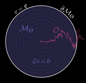
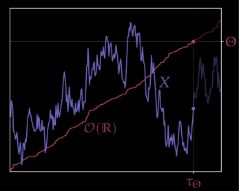
Fig. 5 provides an illustration of the exit time $\tau_{\Theta}$ and the Dirichlet problem (51a)$-$(51b). Note that $\operatorname{\mathcal{O}}_{\tau_{\Theta}}(\operatorname{\mathbb{R}})=\Theta$ (hence $\operatorname{\mathcal{O}}_{\tau_{\Theta}}\in\partial\operatorname{\mathcal{M}}_{\Theta}$) as $t\mapsto\langle X\rangle_{t}=\int_{0}^{t}\sigma(\operatorname{\mathcal{O}}_{u},X_{u})^{2}du$ is continuous. When $b\equiv 0$, then (51a) reads $\sigma^{2}\Big{(}\partial_{o}+\frac{1}{2}\partial_{xx}\Big{)}v=0$ which is equivalent to the heat equation (42a)$-$(42b) when $\sigma$ is positive. This is not surprising as the solution of the associated OSDE is a local martingale, hence a time-changed Brownian motion$-$see again Remark 2.

We finish this section by stating Feynman-Kac’s theorem for functionals of the standard time occupation measure. To this end, consider the standard time OSDE

$$d\tilde{\operatorname{\mathcal{O}}}_{t}=\delta_{X_{t}}dt, \tilde{\operatorname{\mathcal{O}}}_{0}\in\operatorname{\mathcal{M}}$$ , (53a)

$$dX_{t}=b(\tilde{\operatorname{\mathcal{O}}}_{t},X_{t})dt+\sigma(\tilde{\operatorname{\mathcal{O}}}_{t},X_{t})dW_{t},\; X_{0}\in\text{supp}(\tilde{\operatorname{\mathcal{O}}}_{0}).$$ (53b)

The associated generator is $\tilde{\operatorname{\mathcal{L}}}=\partial_{o}+b\partial_{x}+\frac{\sigma^{2}}{2}\partial_{xx}$, akin to standard Itô diffusions where $b=b(t,X_{t}),\ \sigma=\sigma(t,X_{t})$. We finally obtain a direct generalization of Theorem 3.2.

Theorem 3.5.

(Feynman-Kac, standard time) Let $\varphi\mathrel{\mathop{\ordinarycolon}}\operatorname{\mathcal{D}}\to\operatorname{\mathbb{R}}$ with $\varphi(\tilde{\operatorname{\mathcal{O}}}_{T},X_{T})\in L^{1}(\operatorname{\mathbb{Q}})$ and consider the Dirichlet problem

$$\tilde{\operatorname{\mathcal{L}}}v=0, \operatorname{\mathcal{D}}_{T},$$ on (54a)

$$v=\varphi, \partial\!\operatorname{\mathcal{D}}_{T},$$ on (54b)

If (53a)$-$(53b) admits a strong solution and (54a) has a classical solution $v\in\operatorname{\mathcal{C}}^{1,2}(\operatorname{\mathcal{D}})$, then

$$v(o,x)=\operatorname{\mathbb{E}}^{\operatorname{\mathbb{Q}}}[\varphi(\tilde{\operatorname{\mathcal{O}}}_{T}^{o,x},X_{T}^{o,x})],\quad(o,x)\in\overline{\operatorname{\mathcal{D}}_{T}}.$$ (55)

The above results allows to characterize the pricing PDE of financial derivatives entailing the standard time occupation measure; see Section 5.1.

3.5 Discussion: Taylor Expansion

Let us provide some heuristic comments pertaining to Taylor expansions of occupation functionals. We here focus on the standard time occupied processes $(\tilde{\operatorname{\mathcal{O}}},X)$ as it relates more closely to the usual stochastic Taylor expansion [1, 43] and functional Taylor expansion [47, 29]. If $f\in\operatorname{\mathcal{C}}^{1,2}(\operatorname{\mathcal{D}})$, we first deduce from (36) the following Stratonovich’s formula,

$$f(\tilde{\operatorname{\mathcal{O}}}_{t},X_{t}) =f(\tilde{\operatorname{\mathcal{O}}}_{0},X_{0})+\int_{0}^{t}\partial_{o}f(\tilde{\operatorname{\mathcal{O}}}_{u},X_{u})du+\int_{0}^{t}\partial_{x}f(\tilde{\operatorname{\mathcal{O}}}_{u},X_{u})\circ dX_{u},$$ (56)

where $\circ$ indicates Stratonovich integration. As the integrands in (56) are themselves occupation functionals, we may iterate Stratonovich’s formula to derive an expansion when $f$ is regular enough. If $f$ is even real analytic in some sense, we formally obtain the Taylor series,

$$f(\tilde{\operatorname{\mathcal{O}}}_{t},X_{t}) =\sum_{\alpha\in\operatorname{\mathcal{A}}}\partial_{\alpha}f(\tilde{\operatorname{\mathcal{O}}}_{0},X_{0})\operatorname{\mathcal{S}}_{\alpha}(X),$$ (57)

with index set $\operatorname{\mathcal{A}}=\{\varnothing\}\cup\{\alpha=\alpha_{1}\cdots\alpha_{k}\in\{0,1\}^{k}\mathrel{\mathop{\ordinarycolon}}k\geq 1\}$ and notations $\partial_{0}=\partial_{o}$, $\partial_{1}=\partial_{x}$, $\partial_{\varnothing}f=f$. The map $\operatorname{\mathcal{S}}_{\alpha}$, otherwise called signature functional, assigns a path to the Stratonovich iterated integral in the variables $t,x$ (where $0\sim t$, $1\sim x$) where $\alpha$ prescribes the order of integration. As an example, $\operatorname{\mathcal{S}}_{01}(X)=\int_{0}^{t}\int_{0}^{t_{2}}\circ\ dt_{1}\circ dX_{t_{2}}=\int_{0}^{t}udX_{u}$. If $\alpha=\varnothing$, we set $\operatorname{\mathcal{S}}_{\varnothing}\equiv 1$. Similar to stochastic Taylor expansions [1, 43], we may derive more general expressions when $(\tilde{\operatorname{\mathcal{O}}},X)$ solves an occupied SDE as in Section 3.4 with smooth coefficients.

Defining the path functional $F(X)=f(\tilde{\operatorname{\mathcal{O}}}(X),X_{t})$, $X\in\Lambda_{t}$, as in Section 3.2.1, then (57) can be formally rewritten as the functional Taylor series,

$$F(X)=\sum_{\alpha\in\operatorname{\mathcal{A}}}\Delta_{\alpha}F(X_{0})\operatorname{\mathcal{S}}_{\alpha}(X),$$ (58)

with the functional derivatives $\Delta_{0}=\Delta_{t}$ (where we recall that $\Delta_{t}F=\partial_{o}f)$, $\Delta_{1}=\Delta_{x}$, and $\Delta_{\varnothing}f=f$; see [29]. Equation (58) gives a decomposition of any path functional in terms of the signature. On the other hand, the series in (57) reveals an important subtlety: the right-hand side possibly depends on the whole path $X$, hence its chronology, while the left-hand side do not. This suggests the existence of a simplified expansion with basis functionals entailing solely the occupied process. Specifically, we conjecture that there is a family $\{\Phi_{\gamma}\mathrel{\mathop{\ordinarycolon}}\operatorname{\mathcal{D}}\to\operatorname{\mathbb{R}}\}_{\gamma\in\Gamma}$ with index set $\Gamma$ no larger than $\operatorname{\mathcal{A}}$ such that

$$f(\tilde{\operatorname{\mathcal{O}}}_{t},X_{t})=\sum_{\gamma\in\Gamma}\partial_{\gamma}f(\tilde{\operatorname{\mathcal{O}}}_{0},X_{0})\ \Phi_{\gamma}(\tilde{\operatorname{\mathcal{O}}}_{t},X_{t}).$$ (59)

Let us verify (59) for the first- and second-order terms. Assuming $X_{0}=0$ and writing $\partial_{\alpha}f=\partial_{\alpha}f(\tilde{\operatorname{\mathcal{O}}}_{0},X_{0}),\ \operatorname{\mathcal{S}}_{\alpha}=\operatorname{\mathcal{S}}_{\alpha}(X)$ for brevity, then

$$f(\tilde{\operatorname{\mathcal{O}}}_{t},X_{t})\approx\partial_{\varnothing}f\operatorname{\mathcal{S}}_{\varnothing}+\partial_{o}f\operatorname{\mathcal{S}}_{0}+\partial_{x}f\operatorname{\mathcal{S}}_{1}+\partial_{oo}f\operatorname{\mathcal{S}}_{00}+\partial_{xx}f\operatorname{\mathcal{S}}_{11}+\partial_{ox}f\operatorname{\mathcal{S}}_{01}+\partial_{xo}f\operatorname{\mathcal{S}}_{10}.$$ (60)

First, introduce $k=k(\alpha)=(k_{0},k_{1})\in\operatorname{\mathbb{N}}^{2}$ where $k_{i}$ is the number of $i$’s in $\alpha$, $i\in\{0,1\}$. If $\alpha\in\{\varnothing,0,1,00,11\}$, we can then set $\operatorname{\mathcal{S}}_{\alpha}(X)=\Phi_{k(\alpha)}(\operatorname{\mathcal{O}}_{t},X_{t})$ with the monomials

$$\Phi_{k}(o,x)=\frac{o(\operatorname{\mathbb{R}})^{k_{0}}}{k_{0}!}\frac{x^{k_{1}}}{k_{1}!},\quad k\in\operatorname{\mathbb{N}}^{2}.$$

Hence $\Phi_{k}(\tilde{\operatorname{\mathcal{O}}}_{t},X_{t})=\frac{t^{k_{0}}}{k_{0}!}\frac{X_{t}^{k_{1}}}{k_{1}!}$. For the last two terms on the right side of (60), recall the Lie bracket $[\partial_{o},\partial_{x}]=\partial_{xo}-\partial_{ox}$ seen in Section 3.1. Then, we compute,

$$\partial_{ox}f\operatorname{\mathcal{S}}_{01}+\partial_{xo}f\operatorname{\mathcal{S}}_{10} =\partial_{ox}f[\operatorname{\mathcal{S}}_{01}+\operatorname{\mathcal{S}}_{10}]+[\partial_{o},\partial_{x}]f\operatorname{\mathcal{S}}_{10}$$

$$=\partial_{ox}f\underbrace{\left[\int_{0}^{t}sdX_{s}+\int_{0}^{t}X_{s}ds\right]}_{tX_{t}}+[\partial_{o},\partial_{x}]f\int_{0}^{t}X_{s}ds$$

$$=\partial_{ox}f\ \Phi_{(1,1)}(\tilde{\operatorname{\mathcal{O}}}_{t},X_{t})+[\partial_{o},\partial_{x}]f\ \Phi_{10}(\tilde{\operatorname{\mathcal{O}}}_{t},X_{t}),$$

with $\Phi_{k}$ defined above and $\Phi_{10}(o,x)=\int_{\operatorname{\mathbb{R}}}yo(dy)$ from the occupation time formula (10). With a slight abuse of notation, we can write $\Phi_{\gamma}$ whether $\gamma=k\in\operatorname{\mathbb{N}}^{2}$ or $\gamma=\alpha\in\operatorname{\mathcal{A}}$ when $\operatorname{\mathcal{S}}_{\alpha}(X)$ only depend on the path through $(\tilde{\operatorname{\mathcal{O}}}_{t},X_{t})$ such as $\alpha=10$. This includes more generally the sequence $\alpha^{(k)}=1\cdots 10\in\{0,1\}^{k+1}$, $k\in\operatorname{\mathbb{N}}$. Indeed,

$$\Phi_{\alpha^{(k)}}(\tilde{\operatorname{\mathcal{O}}}_{t},X_{t})=\int_{\operatorname{\mathbb{R}}}\frac{x^{k}}{k!}\tilde{\operatorname{\mathcal{O}}}_{t}(dx)=\int_{0}^{t}\frac{X_{s}^{k}}{k!}ds=\operatorname{\mathcal{S}}_{\alpha^{(k)}}(X).$$

Note in passing that the elements $\{\operatorname{\mathcal{S}}_{\alpha^{(k)}}(X)\}_{k\in\operatorname{\mathbb{N}}}$ can approximate the integrals $\int_{0}^{t}\mathds{1}_{A}(X_{s})ds$, $A\in\operatorname{\mathcal{B}}(\operatorname{\mathbb{R}})$, and thus fully characterize the standard time occupation measure itself. It is expected that similar arguments combining integration by parts and the occupation time formula would generate basis occupation functionals of higher orders, yet a precise derivation is beyond the scope of this work.

4 Stopping Spot Local Time

This section intends to study the spot local time $L_{t}^{X_{t}}$ in more depth, particularly in the context of optimal stopping (OS). We dwell on this problem as we believe it is highly challenging both theoretically and numerically. Hence, the stopping of spot local time can be used as a benchmark for algorithms solving path-dependent OS problems. For instance, it would be worth checking the performance on this example of recent methods involving deep learning and/or the path signature [3, 4, 5]. See Section 4.3 for further numerical considerations.

4.1 Optimal Stopping

Let us first adapt standard results in optimal stopping to occupied processes. Suppose that $X$ is Brownian motion and refer to Remark 2 for the general semimartingale case. Given a reward functional $\varphi\mathrel{\mathop{\ordinarycolon}}\operatorname{\mathcal{D}}\to\operatorname{\mathbb{R}}_{+}$ such that $\sup_{t\leq T}\varphi(\operatorname{\mathcal{O}}_{t},X_{t})\in L^{1}(\operatorname{\mathbb{Q}})$ and exercise dates $\operatorname{\mathcal{T}}\subseteq[0,T]$ containing $T$, consider the optimal stopping (OS) problem [50],

$$\sup_{\tau\in\vartheta(\operatorname{\mathcal{T}})}\operatorname{\mathbb{E}}^{\operatorname{\mathbb{Q}}}[\varphi(\operatorname{\mathcal{O}}_{\tau},X_{\tau})],$$ (61)

where $\vartheta(\operatorname{\mathcal{T}})$ is the set of $\operatorname{\mathcal{T}}-$valued $(\operatorname{\mathbb{F}},\operatorname{\mathbb{Q}})-$stopping times. Define the value function,

$$v(o,x)=\sup_{\tau\in\vartheta(\operatorname{\mathcal{T}}_{t})}\operatorname{\mathbb{E}}^{\operatorname{\mathbb{Q}}}_{o,x}[\varphi(\operatorname{\mathcal{O}}_{\tau},X_{\tau})],\quad\operatorname{\mathcal{T}}_{t}=\operatorname{\mathcal{T}}\cap\ [t,T],\quad o(\operatorname{\mathbb{R}})=t,$$ (62)

with $\operatorname{\mathbb{E}}^{\operatorname{\mathbb{Q}}}_{o,x}$ as in (43). The stopping region is traditionally defined as the coincidence set $\operatorname{\mathcal{S}}_{T}=\{(o,x)\in\operatorname{\mathcal{D}}_{T}\mathrel{\mathop{\ordinarycolon}}v(o,x)=\varphi(o,x)\}$. In particular, $\partial\operatorname{\mathcal{S}}=\partial\operatorname{\mathcal{D}}_{T}$ since $T\in\operatorname{\mathcal{T}}$. As it is challenging to represent $\operatorname{\mathcal{S}}$ either mentally or visually, we can regard the stopping region as a subset of $\operatorname{\mathbb{R}}$ for a given occupation measure, i.e., $\operatorname{\mathcal{S}}(o)=\{x\in\text{supp}(o)\ \mathrel{\mathop{\ordinarycolon}}\ (o,x)\in\operatorname{\mathcal{S}}\}$. For every $t\in[0,T]$ , this gives the pathwise partition

$$\{X_{s}\mathrel{\mathop{\ordinarycolon}}s\leq t\}=\text{supp}(\operatorname{\mathcal{O}}_{t})=\operatorname{\mathcal{S}}(\operatorname{\mathcal{O}}_{t})\cup\operatorname{\mathcal{C}}(\operatorname{\mathcal{O}}_{t}),$$

with the continuation region $\operatorname{\mathcal{C}}(o)=\{x\in\text{supp}(o)\ \mathrel{\mathop{\ordinarycolon}}\ v(o,x)>\varphi(o,x)\}$. See Fig. 7 and [25, Chapter 7] for a similar comment.

Dynamic Programming Equation. The Dynamic Programming Principle (DPP) states that for every stopping time $\varsigma\in\vartheta(\operatorname{\mathcal{T}}_{t})$,

$$v(o,x) =\sup_{\tau\in\vartheta(\operatorname{\mathcal{T}}_{t})}\ \operatorname{\mathbb{E}}^{\operatorname{\mathbb{Q}}}_{o,x}[\varphi(\operatorname{\mathcal{O}}_{\tau},X_{\tau})\mathds{1}_{\{\tau<\varsigma\}}+v(\operatorname{\mathcal{O}}_{\varsigma},X_{\varsigma},)\mathds{1}_{\{\tau\geq\varsigma\}}].$$ (63)

Let us recall how to derive the dynamic programming equation satisfied by $v$. If $v\in\operatorname{\mathcal{C}}^{1,2}(\operatorname{\mathcal{D}})$ and $Y_{t}\mathrel{\mathop{\ordinarycolon}}=v(\operatorname{\mathcal{O}}_{t},X_{t})$ denotes the Snell envelope of $\varphi$, then Itô’s formula (Theorem 3.1) gives

$$dY_{t} =\Big{(}\partial_{o}+\frac{1}{2}\partial_{xx}\Big{)}v(\operatorname{\mathcal{O}}_{t},X_{t})dt+\partial_{x}v(\operatorname{\mathcal{O}}_{t},X_{t})dX_{t}.$$ (64)

It is classical that the Snell envelope $Y$ is the smallest supermartingale dominating $\varphi$ [50]. In particular, the drift in (64) is $\operatorname{\mathbb{Q}}-$a.s. non-positive and equal to zero outside of the stopping region $\operatorname{\mathcal{S}}$. This leads to the dynamic programming equation,

$$\Big{(}\partial_{o}+\frac{1}{2}\partial_{xx}\Big{)}v=0 \operatorname{\mathcal{D}}_{T}$$ on, (65a)

$$v=\varphi \ \operatorname{\mathcal{S}}_{T}\cup\ \partial\operatorname{\mathcal{D}}_{T}.$$ on (65b)

The present discussion of course formal as the value function is typically not regular enough to be a classical solution of (65a)$-$(65b). Similar to [53, 54] in the context of mean-field optimal stopping, it is expected that an extension of the classical viscosity theory [31] will give positive answers. This is nevertheless subject to future research.

Figure 6: Flow of occupation measures $\operatorname{\mathcal{O}}$ and stopped spot local time $L_{\tau}^{X_{\tau}}$. Two simulations.

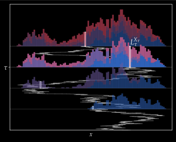
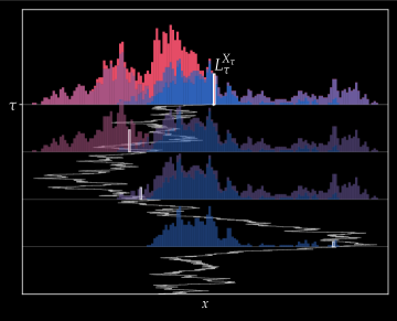
4.2 Spot Local Time and Early Exercise Premium

We are now set to study the OS problem,

$$\text{maximize }\;v(\tau)\mathrel{\mathop{\ordinarycolon}}=\operatorname{\mathbb{E}}^{\operatorname{\mathbb{Q}}}[L_{\tau}^{X_{\tau}}]\;\;\text{ over }\;\tau\in\vartheta(\operatorname{\mathcal{T}}).$$ (66)

The spot local time corresponds to the reward $\varphi(o,x)=\frac{do}{d\lambda}(x)$ which is defined on $\operatorname{\mathcal{D}}^{\lambda}$, namely those elements $(o,x)$ of $\operatorname{\mathcal{D}}$ such that $o\in\operatorname{\mathcal{M}}^{\lambda}$. Clearly, $\sup_{t\leq T}\varphi(\operatorname{\mathcal{O}}_{t},X_{t})\in L^{1}(\operatorname{\mathbb{Q}})$ since $\varphi(\operatorname{\mathcal{O}}_{t},X_{t})\leq\lVert\operatorname{\mathcal{O}}_{T}\rVert_{\infty}=\sup_{x\in\operatorname{\mathbb{R}}}L_{T}^{x}$ which is bounded in $L^{p}(\operatorname{\mathbb{Q}})$ for all $p\geq 1$ [2]. Hence the above OS problem is well-defined. Within the family of metrics $\{\operatorname{\mathfrak{m}}_{p}\mathrel{\mathop{\ordinarycolon}}p\in[1,\infty]\}$ introduced in Section 2.1, note that $\varphi$ is continuous only with respect to $\operatorname{\mathfrak{m}}_{\infty}$.

It is intuitive that (66) has a positive early exercise premium when $\operatorname{\mathcal{T}}\neq\{T\}$ (recall our assumption $T\in\operatorname{\mathcal{T}}$). See also Fig. 6. In other words, there exists $\tau\in\vartheta(\operatorname{\mathcal{T}})$ such that $v(\tau)$ strictly dominates $v(T)=\operatorname{\mathbb{E}}^{\operatorname{\mathbb{Q}}}[L_{T}^{X_{T}}]$. First, let us compute the latter explicitly.

Proposition 5.

Let $X$ be Brownian motion and $T>0$. Then $\operatorname{\mathbb{E}}^{\operatorname{\mathbb{Q}}}[L_{T}^{X_{T}}]=\operatorname{\mathbb{E}}^{\operatorname{\mathbb{Q}}}[L_{T}^{0}]=\sqrt{\frac{2}{\pi}T}$.

Proof.

Consider the time reversed process $\overleftarrow{X}_{s}=X_{T-s}-X_{T}$, $s\in[0,T]$ and denote its local time at $0$ by $\overleftarrow{L^{0}}$. By the chronology invariance of occupation functionals (Theorem 2.1), then $L_{T}^{X_{T}}=\overleftarrow{L^{0}_{T}}$ pathwise. Moreover, it is classical that $\overleftarrow{X}$ is also Brownian motion with respect to its own filtration, hence $\operatorname{\mathbb{E}}^{\operatorname{\mathbb{Q}}}[L_{T}^{X_{T}}]=\operatorname{\mathbb{E}}^{\operatorname{\mathbb{Q}}}[\overleftarrow{L^{0}_{T}}]=\operatorname{\mathbb{E}}^{\operatorname{\mathbb{Q}}}[L_{T}^{0}]$. The last equality in the statement follows from the standard result from Paul Lévy that $L_{T}^{0}$ and $|X_{T}|$ have the same law. ∎

Next, we verify the existence of an early exercise premium in the minimal case $\operatorname{\mathcal{T}}=\{t,T\}$. Invoking the dynamic programming principle (63) with $\varsigma=T$, then $Y_{t}\mathrel{\mathop{\ordinarycolon}}=v(\operatorname{\mathcal{O}}_{t},X_{t})=L_{t}^{X_{t}}\vee C_{t}$ with the continuation value $C_{t}=\operatorname{\mathbb{E}}^{\operatorname{\mathbb{Q}}}[L_{T}^{X_{T}}|\operatorname{\mathcal{F}}_{t}]$ derived in Example 6, namely

$$C_{t}=\int_{\operatorname{\mathbb{R}}}L_{t}^{y}\ \phi_{T-t}(y-X_{t})dy+\operatorname{\mathbb{E}}^{\operatorname{\mathbb{Q}}}[L_{T-t}^{0}],\quad\phi_{s}(x)=\frac{e^{-\frac{x^{2}}{2s}}}{\sqrt{2\pi s}}.$$ (67)

We can finally approximate the initial value $Y_{0}=\operatorname{\mathbb{E}}^{\operatorname{\mathbb{Q}}}[Y_{t}]$ using Monte Carlo simulations. For the numerical computation of the local times in (67), see Remark 8. The optimal strategy is classically to stop at $t$ if the intrinsic value $L_{t}^{X_{t}}$ is greater than equal to $C_{t}$; see Fig. 7. As the heat kernel $\phi_{T-t}$ concentrates around zero (especially when $T-t$ is small), we gather from (67) that the field $(L_{t}^{x})_{x\in\operatorname{\mathbb{R}}}$ is relevant for the stopping decision only in a neighborhood of the spot. This observation is crucial in Section 4.3 when truncating the occupation measure.

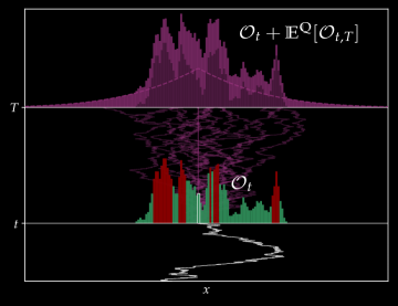
Figure 7: Spot local time OS problem with $\operatorname{\mathcal{T}}=\{t,T\}$. Stopping region (red) and continuation region (green) at $t$ depending whether the intrinsic value $L_{t}^{x}$ (if $X_{t}=x$) exceeds the continuation value given in (67).

Table 1 summarizes the results in the case $T=2t=1$. We simulate $2^{14}=16,384$ Monte Carlo paths on a regular time grid with $N=400$ steps and set $\varepsilon=\sqrt{T/N}=0.05$; see Remark 8. The early exercise premium is indeed significantly positive.

Table 1: Existence of an early exercise premium. Value of the OS problem (66) with $\operatorname{\mathcal{T}}=\{0.5,1\}$ and $\operatorname{\mathcal{T}}=\{1\}$. $N=400$, $\varepsilon=0.05$, and $2^{14}$ Monte Carlo (MC) simulations.

Exercise dates	Value	MC Error
$\operatorname{\mathcal{T}}=\{0.5,1\}$	0.8455	0.0050
$\operatorname{\mathcal{T}}=\{1\}$	0.7979	-

Remark 8.

(Numerical approximation of Brownian local time) Define

$$\varphi^{\varepsilon}(\operatorname{\mathcal{O}}_{t},x)\mathrel{\mathop{\ordinarycolon}}=\frac{\operatorname{\mathcal{O}}_{t}(B_{\varepsilon}(x))}{2\varepsilon}=\frac{1}{2\varepsilon}\int_{0}^{t}\mathds{1}_{\{|X_{s}-x|\leq\varepsilon\}}ds.$$ (68)

In light of (11), $\varphi^{\varepsilon}(\operatorname{\mathcal{O}}_{t},x)$ converges to $L_{t}^{x}$ pathwise. In the present context of optimal stopping, we shall also see in Section 4.4 that estimating local time with narrow corridors is legitimate in the sense that the value of the OS problem (61) with $\varphi=\varphi^{\varepsilon}$ converges to the value of (66). If $X$ is a simulated Brownian path on a regular time grid $t_{n}=n\delta t$, $\delta t=\frac{T}{N}$, we then discretize the integral in (68) to obtain $L_{t}^{x}\approx\frac{1}{2\varepsilon}\sum_{n=1}^{N}\mathds{1}_{\{|X_{t_{n}}-x|\leq\varepsilon\}}\delta t.$ This estimate induces constraints on $\varepsilon$ once $\delta t$ is fixed. Intuitively, $\varepsilon\gg\delta t$, and from our experiments, adequate choices are $\varepsilon=c\sqrt{\delta t}$, e.g. $c=1$, matching the scale of Brownian motion.

4.3 Numerical Resolution in the case $\operatorname{\mathcal{T}}=[0,T]$

We now turn to the case $\operatorname{\mathcal{T}}=[0,T]$. As the backward induction in the previous section does not apply when $|\operatorname{\mathcal{T}}|>2$ due to path-dependence, alternative methods must be considered. First, we outline a simple stopping rule giving a lower bound on the value of (66).

Inspection Strategy. For fixed $\iota\in[0,T]$, interpreted as an inspection date, define

$$\tau_{\iota}=\inf\{t\in[\iota,T]\ \mathrel{\mathop{\ordinarycolon}}\ X_{t}=X^{*}_{\iota}\}\wedge T,\quad X^{*}_{\iota}=\text{argmax}_{x}L_{\iota}^{x}.$$

In other words, it is the hitting time after $\iota$ of the level which maximizes local time on $[0,\iota]$. If $\sigma^{*}=\sup\{s\in[0,T]\mathrel{\mathop{\ordinarycolon}}X_{s}=X^{*}_{\iota}\}\wedge 0$ denotes the last visit of the optimal level $X_{\iota}^{*}$, then on $\{\sigma^{*}\geq\iota\}$, the reward $L_{\tau_{\iota}}^{X_{\iota}^{*}}$ is precisely $L_{\iota}^{X_{\iota}^{*}}=\sup_{x}L_{\iota}^{x}$. This gives the decomposition,

$$\operatorname{\mathbb{E}}^{\operatorname{\mathbb{Q}}}[L_{\tau_{\iota}}^{X_{\tau_{\iota}}}]=p_{\iota}\operatorname{\mathbb{E}}^{\operatorname{\mathbb{Q}}}[\sup_{x}L_{\iota}^{x}\ |\ \sigma^{*}\geq\iota]+(1-p_{\iota})\operatorname{\mathbb{E}}^{\operatorname{\mathbb{Q}}}[L_{T}^{X_{T}}\ |\ \sigma^{*}<\iota],\quad p_{\iota}=\operatorname{\mathbb{Q}}(\sigma^{*}\geq\iota).$$

There is a clear tradeoff between the reward $\sup_{x}L_{\iota}^{x}$ (increasing in $\iota$) and the probability $p_{\iota}$ to hit the level $X^{*}_{\iota}$ again (decreasing in $\iota$). Table 2 summarizes the numerical results for values of $\iota$. We use $T=1$ and $2^{14}=16,384$ simulated Brownian trajectories on a regular time grid with $400$ steps. To compute $X_{\iota}^{*}$, we use a regular space grid of $[-2,2]$ with $200$ subintervals. Despite the simplicity of the present stopping rule, a significant premium is observed. Note that the inspection date $\iota=0.7$ yields nearly a $40\%$ improvement over the case $\operatorname{\mathcal{T}}=\{T\}$ seen in Table 1.

Table 2: Value of the stopping rule $\tau_{\iota}=\inf\{t\in[\iota,T]\ \mathrel{\mathop{\ordinarycolon}}\ X_{t}=X^{*}_{\iota}\}$, $X^{*}_{\iota}=\text{argmax}_{x}L_{\iota}^{x}$ for varying inspection date $\iota$ and parameters $T=1$, $N=400$, $\varepsilon=0.05$.

Inspection date	Value	Monte Carlo Error
$\iota=0.5$	1.0404	0.0035
$\iota=0.6$	1.0897	0.0040
$\iota=0.7$	1.1116	0.0046
$\iota=0.8$	1.0892	0.0052
$\iota=0.9$	1.0182	0.0056

Least Square Monte Carlo. We now implement an approach à la Longstaff-Schwartz where we refer to the original paper [48] and Section B.2 for further details. Given the time grid $t_{n}=n\delta t,\ \delta t=\frac{T}{N}$, a crucial step in [48] is the computation of the continuation value $C_{t_{n}}=\operatorname{\mathbb{E}}^{\operatorname{\mathbb{Q}}}[Y_{t_{n+1}}|\operatorname{\mathcal{F}}_{t_{n}}]$ where $Y=v(\operatorname{\mathcal{O}},X)$ denotes the Snell envelope of $L^{X}$. Although we can write $C_{t_{n}}=c(\operatorname{\mathcal{O}}_{t_{n}},X_{t_{n}})$, $c\mathrel{\mathop{\ordinarycolon}}\operatorname{\mathcal{D}}\to\operatorname{\mathbb{R}}$, using the Markov property of $(\operatorname{\mathcal{O}},X)$ (Proposition 2), it is naturally challenging to estimate $c$ as the occupation measure is infinite-dimensional. Therefore, we carry out a space discretization to summarize $\operatorname{\mathcal{O}}$ with finitely many features.

Given $\nu=\frac{1}{6}\big{(}\delta_{-\sqrt{3}}+4\delta_{0}+\delta_{\sqrt{3}}\big{)}$ matching the first five moments of $\mathcal{N}(0,1)$, introduce the random walk $X_{t_{n+1}}=X_{t_{n}}+Z_{n+1}\sqrt{\delta t},\ Z_{n+1}\sim\nu,$ taking values on a trinomial tree with nodes $x_{m}=m\sqrt{3\delta t}$ and $|m|\leq n$ at time $t_{n}$. In this model, the occupation measure becomes finite-dimensional, namely

$$\operatorname{\mathcal{O}}_{t_{n}}=(L_{t_{n}}^{x_{-n}},\ldots,L_{t_{n}}^{0},\ldots,L_{t_{n}}^{x_{n}}),\quad L_{t_{n}}^{x_{m}}=\frac{\operatorname{\mathcal{O}}_{t_{n}}(B_{\varepsilon}(x_{m}))}{2\varepsilon}\mathrel{\mathop{\ordinarycolon}}=\frac{1}{2\varepsilon}\sum_{i=1}^{n}\mathds{1}_{\{X_{t_{i}}\ =\ x_{m}\}}\delta t.$$ (69)

where $\varepsilon=\frac{x_{m+1}-x_{m}}{2}=\frac{\sqrt{3\delta t}}{2}$ in line with Remark 8. The above expression for $L_{t_{n}}^{x_{m}}$ also reveals our motivation behind the chosen trinomial structure: the local time process may accumulate at every step instead of every other step in a (recombining) binomial tree.

Notice that the dimension of $\operatorname{\mathcal{O}}_{t_{n}}$ in (69) still expands with time, which becomes problematic for large $N$. Therefore, we introduce the truncation $\operatorname{\mathcal{O}}_{t_{n}}^{\bar{m}}=(L_{t_{n}}^{x_{m-\bar{m}}},\ldots,L_{t_{n}}^{x_{m+\bar{m}}})$, $\bar{m}\in\operatorname{\mathbb{N}}$, around the spot $x_{m}=X_{t_{n}}$. The resulting pair $(\operatorname{\mathcal{O}}_{t_{n}}^{\bar{m}},X_{t_{n}})$ is of dimension $2\bar{m}+2$, hence a least square approach can be implemented for small values of $\bar{m}$ (say, less than $5$). Note that this is tailored to the payoff $L^{X}$: similar to (67), the continuation value primarily depends on the local time close to the spot. Evidently, other rewards may lead to other truncations.

We then follow the least square Monte Carlo method [48], expounded in Algorithm 1 for completeness. We perform an offline and online phase as in [38, Remark 6.8] consisting of $2^{11}$ and $2^{14}$ simulations, respectively. See also Section B.2 for other implementation details. The results are given in Table 3. Note that adding the local time of adjacent nodes ($\bar{m}=1$) is indeed benefical, while the value improves slowly beyond that. Comparing with Table 2, we also see that the least square Monte Carlo approach indeed outperforms the more naive inspection strategy.

Table 3: Value of OS problem (66) with $\operatorname{\mathcal{T}}=\{n/N\mathrel{\mathop{\ordinarycolon}}n=1,\ldots,N\}$, $N=400$, using Least square Monte Carlo for varying truncation level $\bar{m}$.

Truncation level $(\bar{m})$	Value	MC Error	Run time
$0$	1.1916	0.0044	182 sec.
$1$	1.2180	0.0031	187 sec.
$2$	1.2252	0.0030	194 sec.
$3$	1.2277	0.0030	197 sec.
$5$	1.2296	0.0030	210 sec.

4.4 Shrinking the Corridor

Let $\varphi^{\varepsilon}(o,x)=\frac{o(B_{\varepsilon}(x))}{2\varepsilon}$, $\varepsilon>0$ as in (68). Hence $\varphi^{\varepsilon}(X_{t},\operatorname{\mathcal{O}}_{t})$ is a pathwise approximation of the spot local time $L_{t}^{X_{t}}$. We aim to show that the value $v_{*}^{\varepsilon}$ of the optimal stopping problem

$$\text{maximize }\;v^{\varepsilon}(\tau)\mathrel{\mathop{\ordinarycolon}}=\operatorname{\mathbb{E}}^{\operatorname{\mathbb{Q}}}[\varphi^{\varepsilon}(\operatorname{\mathcal{O}}_{\tau},X_{\tau})]\;\;\text{ over }\;\tau\in\vartheta(\operatorname{\mathcal{T}}),$$ (70)

converges to the value $v_{*}$ of (66) in the extremes cases $\operatorname{\mathcal{T}}=\{T\}$ and $\operatorname{\mathcal{T}}=[0,T]$. We start with the former, where $v_{*}^{\varepsilon}=v^{\varepsilon}(T)$ and $v_{*}=v(T)$.

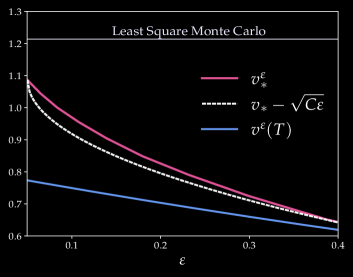
Figure 8: Verification of Proposition 6 and Corollary 1 with $T=1$. Estimate of $\varepsilon\mapsto v_{*}^{\varepsilon}$ using the inspection strategy (Section 4.3), $N=400$ time intervals and $2^{14}$ simulations. Comparison with the function $v_{*}-\sqrt{C\varepsilon}$ for some $C\in(0,\infty)$ and the European price $v^{\varepsilon}(T)$. The value using least square Monte Carlo is also reported.

Proposition 6.

We have $v^{\varepsilon}(T)\uparrow v(T)$ as $\varepsilon\downarrow 0$. Precisely, $v^{\varepsilon}(T)=v(T)-\frac{\varepsilon}{2}+\frac{\varepsilon^{2}}{\sqrt{18\pi T}}(1+r_{\varepsilon})$ with $\lim_{\varepsilon\downarrow 0}r_{\varepsilon}=0$.

Proof.

See Section A.5. ∎

We gather from Proposition 6 that the function $\varepsilon\mapsto v^{\varepsilon}(T)$ is essentially linear for small values of $\varepsilon$. This will be confirmed in Fig. 8. In the next results, we prove that the convergence rate of $v^{\varepsilon}(\tau)$ for general stopping times and $v_{*}^{\varepsilon}$ when $\operatorname{\mathcal{T}}=[0,T]$ is at least $1/2$. In fact, this lower bound seems tight according to Fig. 8.

Proposition 7.

There exists a constant $C\in(0,\infty)$ such that for all $0<\varepsilon\leq 1$,

$$\left\lVert\varphi^{\varepsilon}(\operatorname{\mathcal{O}}_{\tau},X_{\tau})-L_{\tau}^{X_{\tau}}\right\rVert_{L^{2}(\operatorname{\mathbb{Q}})}\leq\sqrt{C\varepsilon}\qquad\forall\tau\in\vartheta(\operatorname{\mathcal{T}}).$$ (71)

In particular, $|v^{\varepsilon}(\tau)-v(\tau)|\leq\sqrt{C\varepsilon}$ for all $\tau\in\vartheta(\operatorname{\mathcal{T}})$.

Proof.

See Section A.6. ∎

Corollary 1.

Let $v_{*}^{\varepsilon}$, $v_{*}$ be respectively the value of the OS problem (70) and (66) with $\operatorname{\mathcal{T}}=[0,T]$. Then $|v^{\varepsilon}_{*}-v_{*}|\leq\sqrt{C\varepsilon}$, with $C$ as in Proposition 7. In particular, $\lim_{\varepsilon\to 0}v_{*}^{\varepsilon}=v_{*}$.

Proof.

This is immediate: let $\gamma>0$ be arbitrary and $\tau_{\gamma}$ such that $v(\tau_{\gamma})\geq v_{*}-\gamma$. Then

$$v_{*}-\gamma\leq v(\tau_{\gamma})\leq v^{\varepsilon}(\tau_{\gamma})+\sqrt{C\varepsilon}\leq v_{*}^{\varepsilon}+\sqrt{C\varepsilon},$$

so $v_{*}-v_{*}^{\varepsilon}\leq\sqrt{C\varepsilon}$ as $\gamma\to 0$. The inequality $v_{*}^{\varepsilon}-v_{*}\leq\sqrt{C\varepsilon}$ is shown mutatis mutandis. ∎

Fig. 8 displays the optimal value of (66) as function of $\varepsilon$ in the case $\operatorname{\mathcal{T}}=\{1\}$ and $\operatorname{\mathcal{T}}=[0,1]$. The highest value from Table 3 using the least square Monte Carlo approach is also reported. We use the inspection strategy laid out in Section 4.3 to estimate the value in the case $\operatorname{\mathcal{T}}=[0,1]$. Note that the early exercise premium (spread between the magenta and blue lines) is significant and increases as the corridor width shrinks to zero. This is because peaks in the local time field $x\mapsto L_{t}^{x}$ can be captured more accurately as $\varepsilon$ gets smaller.

5 Financial Examples

Occupied processes appear frequently in finance. As we shall see in Sections 5.1 and 5.4, It is sometimes preferable to consider the standard time occupation measure $\tilde{\operatorname{\mathcal{O}}}$ (or variations of it; see Example 10) instead of $\operatorname{\mathcal{O}}$. The latter is nevertheless crucial for timer options and corridor variance swaps as exemplified in Sections 5.2 and 5.3, respectively.

5.1 Exotic Derivatives

We gather examples of exotic options where the payoff can be expressed in terms of a standard time occupation functional. If $X$ represent the price of the underlying asset and $\operatorname{\mathbb{Q}}$ is a risk-neutral measure, then the European price of an exotic option with payoff $\varphi=\varphi(\tilde{\operatorname{\mathcal{O}}}_{T},X_{T})$ at time $t$ is given by $v(\tilde{\operatorname{\mathcal{O}}_{t}},X_{t})=\operatorname{\mathbb{E}}^{\operatorname{\mathbb{Q}}}[\varphi(\tilde{\operatorname{\mathcal{O}}}_{T},X_{T})\ |\operatorname{\mathcal{F}}_{t}]$. We here assume zero interest rate for simplicity, although discount factors can be theoretically absorbed by the functional $\varphi$ as $\tilde{\operatorname{\mathcal{O}}_{t}}(\operatorname{\mathbb{R}})=t$. If the asset follows the dynamics of an occupied SDE as in (53b) (see also Section 5.4) we can then invoke Feynman-Kac’s formula for standard time occupied processes (Theorem 3.5) to deduce the pricing PDE solved by $v$.

Let us start with commonly traded exotic derivatives, namely Asian and lookback options. Although viewing these products through the lens of occupied processes may be overkill, it is still worth mentioning that they belong to our framework.

Example 7.

(Asian options) These are contracts contingent upon the running average of the underlying, that is $\frac{1}{{T}}\int_{0}^{T}X_{t}dt$. Clearly, the chronology is irrelevant and from the occupation time formula, we have that $\int_{0}^{T}X_{t}dt=\int_{\operatorname{\mathbb{R}}}xd\tilde{\operatorname{\mathcal{O}}}_{T}$. We can therefore express any Asian-type option in terms of the (standard time) occupation measure as well as the spot price when need be. For instance, the payoff of an floating strike Asian call reads

$$\left(X_{T}-\frac{1}{{T}}\int_{0}^{T}X_{t}dt\right)^{+}=\left(X_{T}-\frac{1}{\tilde{\operatorname{\mathcal{O}}}_{T}(\operatorname{\mathbb{R}})}\int_{\operatorname{\mathbb{R}}}xd\tilde{\operatorname{\mathcal{O}}}_{T}\right)^{+}=\varphi(\tilde{\operatorname{\mathcal{O}}}_{T},X_{T}).$$

Example 8.

(Lookback options) A derivative of lookback type entails the running maximum, minimum or range of the underlying asset. Any of these quantities can be retrieved from the occupation measure $\operatorname{\mathcal{O}}$ (or $\tilde{\operatorname{\mathcal{O}}}$) as seen for the maximum in Example 3. As an illustration, the payoff of a floating lookback put option can be expressed as

$$\left(X_{T}-\min_{t\leq{T}}X_{t}\right)^{+}=(X_{T}-m(\operatorname{\mathcal{O}}_{T}))^{+}=\varphi(\operatorname{\mathcal{O}}_{T},X_{T}),\quad m(o)=\inf\textnormal{supp}(o).$$

We end this section with a popular class of contracts in the quantitative finance literature known as occupation time derivatives [17, 42] [25, Chapter 7]. The generic form for the payoff of such options is

$$\varphi(\tilde{\operatorname{\mathcal{O}}}_{T},X_{T})=\phi(\tilde{\operatorname{\mathcal{O}}}_{T}(A),X_{T}),\quad\phi\mathrel{\mathop{\ordinarycolon}}\operatorname{\mathbb{R}}^{2}\to\operatorname{\mathbb{R}},\quad A\in\operatorname{\mathcal{B}}(\operatorname{\mathbb{R}}).$$ (72)

The crucial distincion between payoffs as in (72) and occupation functionals is that the former depends on the occupation measure solely through the occupation time of a specific Borel set. For these derivatives, it is therefore sufficient to consider the two-dimensional process $(\tilde{\operatorname{\mathcal{O}}}(A),X)$ which naturally simplifies the analysis. See [25, Chapter 7] for a review of occupation time derivatives (of both European and American type) and Example 9 below.

Example 9.

(Parisian barrier options and soft call provision) Barrier options are contracts with a knock-in (creation) or knock-out (termination) feature that is activated if the underlying asset breaches a prescribed level$-$ the barrier. As the range of the asset $X$ coincide with the support of its occupation measure ($\tilde{\operatorname{\mathcal{O}}}$ or $\operatorname{\mathcal{O}}$), the payoff of barrier options can be expressed in terms of an occupation functional of the form $\varphi(\operatorname{\mathcal{O}}_{T},X_{T})=\psi(\text{supp}(\operatorname{\mathcal{O}}_{T}),X_{T})$ for some $\psi\mathrel{\mathop{\ordinarycolon}}\operatorname{\mathcal{B}}(\operatorname{\mathbb{R}})\times\operatorname{\mathbb{R}}\to\operatorname{\mathbb{R}}_{+}$. Alternatively, any barrier option can be expressed as an occupation time derivative (72). For example, an up-and-out digital option with barrier $b>0$ admits the $\operatorname{\mathbb{Q}}-$almost sure representation,

$$\mathds{1}_{\{X_{t}\ <\ b\ \forall\ t\ \leq\ {T}\}}=\mathds{1}_{\{\tilde{\operatorname{\mathcal{O}}}_{T}(A^{b})\ =\ 0\}}=\phi(\tilde{\operatorname{\mathcal{O}}}_{T}(A^{b})),\quad A^{b}=[b,\infty).$$ (73)

Later, Parisian options [17, 42] have been introduced to soften barrier options. Precisely, the knock-in/out component is triggered only once the asset stays above/below the barrier for a given amount of time $\delta>0$, referred to as the window. Some contracts require that the cumulative time above/below the barrier exceeds the window or that there is one excursion of length at least $\delta$ in the activation region. As the latter case depends on the chronology of the path, only the former specification can be characterized by occupation functionals in view of Theorem 2.1. In the case of a cumulative Parisian option, the payoff in (73) is therefore replaced by

$$\mathds{1}_{\{\tilde{\operatorname{\mathcal{O}}}_{T}(A^{b})\ <\ \delta\}}=\phi_{\delta}(\tilde{\operatorname{\mathcal{O}}}_{T}(A^{b})).$$ (74)

The introduction of a window is particularly appealing to the buyer of knock-out Parisian options as it prevents the contracts to become worthless if the asset touches the barrier only once. From the seller’s perspective, Parisian options are easier to hedge as the soft barrier effectively smoothen the Greeks. Other instruments exhibit a similar relaxation feature. One example is the soft call provision for fixed income products such as convertible bonds, where the issuer discontinues (calls) the contract once the underlying has spent a certain amount of time above a threshold.

5.2 Timer Options

Introduced by Société Générale Corporate & Investment Banking in 2007 [52], timer options [7], [38, Chapter 1] allow investors to preselect the level of volatility to value the contract. That is, the terminal payoff is delivered once the realized variance reaches a prescribed budget. The main advantage of these contracts is that the buyer can save the premium (typically positive) between implied volatility used to price the option and realized volatility.

Let $S$ be an asset with dynamics $dS_{t}=\sigma_{t}S_{t}dW_{t}$, $\sigma_{t}\geq\underline{\sigma}>0$ and denote its log price by $X$. Define also the quadratic variation (or total variance) process $Q_{t}=\langle X\rangle_{t}=\int_{0}^{t}\sigma_{s}^{2}ds$ and $\tau_{q}=\inf\{t\geq 0\mathrel{\mathop{\ordinarycolon}}Q_{t}\geq q\}$. Given a payoff $\varphi$ and budget $\bar{q}>0$, it is easy to see using $d\langle S\rangle_{t}=S_{t}^{2}dQ_{t}$ and Itô’s formula that the price function $u(q,s)\mathrel{\mathop{\ordinarycolon}}=\operatorname{\mathbb{E}}^{\operatorname{\mathbb{Q}}}[\varphi(S_{\tau_{\bar{q}-q}})\ |\ S_{0}=s]$ (taking zero interest rates) solves the PDE

$$\Big{(}\partial_{q}+\frac{s^{2}}{2}\partial_{ss}\Big{)}u(q,s)=0, q<\bar{q}$$ , (75a)

$$u(q,s)=\varphi(s) q=\bar{q}.$$ (75b)

Note that the volatility does not appear in (75a) as it is absorbed by the quadratic variation process. Consequently, the value of the contract is insensitive to the volatility in the dynamics of $S$. Unlike most derivatives, timer options do not expose the buyer or seller to vega risk, a feature which is naturally appealing. We also see in (75a) that $Q$ plays the role of time, as does the occupation measure. Hence, the PDE solved by $u$ should relate to the Dirichlet problem (51a)-(51b) as we now explain.

If $\operatorname{\mathcal{O}}$ is the flow of occupation measures associated to the log price $X$, then $Q_{t}=\operatorname{\mathcal{O}}_{t}(\operatorname{\mathbb{R}})$ and we set $v(o,x)\mathrel{\mathop{\ordinarycolon}}=u(o(\operatorname{\mathbb{R}}),e^{x})$. Thus $\partial_{x}v=s\partial_{s}u$, $\partial_{xx}v=s^{2}\partial_{ss}u$, and as in Example 2, $\partial_{o}v=\partial_{q}u$. If the volatility process satisfies $\sigma_{t}=\sigma(\operatorname{\mathcal{O}}_{t},X_{t})$ for some functional $\sigma\mathrel{\mathop{\ordinarycolon}}\operatorname{\mathcal{D}}\to[\underline{\sigma},\infty)$ (see Section 5.4), then $dX_{t}=-\frac{1}{2}\sigma(\operatorname{\mathcal{O}}_{t},X_{t})^{2}dt+\sigma(\operatorname{\mathcal{O}}_{t},X_{t})dW_{t}$ and according to Theorem 3.4, $v$ solves (51a)$-$(51b) with generator $\operatorname{\mathcal{L}}=\sigma^{2}\partial_{o}-\frac{\sigma^{2}}{2}\partial_{x}+\frac{\sigma^{2}}{2}\partial_{xx}$. As expected, we can factor out $\sigma^{2}$ from $\operatorname{\mathcal{L}}$, again confirming the irrelevance of the volatility chosen to price the option.

5.3 Corridor Variance Swaps and Implied Expected Occupation Measure

Corridor Variance Swaps (CVS) are over-the-counter instruments providing exposure to the volatility of an asset when the latter lies within a prescribed range. They belong to the larger family of weighted variance swaps; see Bergomi [6, Chapter 5], Lee [45]. For concreteness, consider an asset $X$ with Bachelier-type dynamics $dX_{t}=\sigma_{t}dW_{t}$, where $W$ is Brownian motion under a risk neutral measure $\operatorname{\mathbb{Q}}$ and $\sigma$ is the volatility process. The profit and loss (P&L) for the holder at expiry date is then given by

$$\text{P\&L}=\underbrace{\frac{1}{T}\int_{0}^{T}\mathds{1}_{[x_{1},x_{2}]}(X_{t})\ \sigma_{t}^{2}dt}_{\text{Floating Leg}}\;\ -\;\ \underbrace{K^{2}_{x_{1},x_{2}}}_{\mathclap{\text{Fixed Leg}}}\ ,\qquad x_{1}<x_{2}.$$ (76)

The levels $x_{1},x_{2}$ defines the corridor during which the instanteneous variance $\sigma_{t}^{2}$ is accumulated while $K_{x_{1},x_{2}}$ is the fair strike usually expressed in volatility terms. The latter is set such that the swap contract has zero initial cost, namely

$$K^{2}_{x_{1},x_{2}}=\operatorname{\mathbb{E}}^{\operatorname{\mathbb{Q}}}\left[\frac{1}{T}\int_{0}^{T}\mathds{1}_{[x_{1},x_{2}]}(X_{t})\ \sigma_{t}^{2}dt\right].$$ (77)

If $\operatorname{\mathcal{O}}$ denotes the occupation measure of $X$, we directly see that

$$\int_{0}^{T}\mathds{1}_{[x_{1},x_{2}]}(X_{t})\sigma_{t}^{2}dt=\int_{0}^{T}\mathds{1}_{[x_{1},x_{2}]}(X_{t})d\langle X\rangle_{t}=\operatorname{\mathcal{O}}_{T}([x_{1},x_{2}]).$$ (78)

The floating leg in (76) thus corresponds to the functional $\varphi(o)=\frac{o([x_{1},x_{2}])}{T}$. Although the maturity $T$ is not directly available from the occupation measure, it is naturally known from the term sheet. There is a well-known connection between corridor variance swaps and local time [6, 45]. Indeed, choosing the levels $x_{1,2}=x\pm\varepsilon$ for some $x\in\operatorname{\mathbb{R}}$, then the scaled floating leg $\frac{1}{2\varepsilon}\int_{0}^{T}\mathds{1}_{[x_{1},x_{2}]}(X_{t})\ \sigma_{t}^{2}dt=\frac{\operatorname{\mathcal{O}}_{T}(\overline{B_{\varepsilon}(x)})}{2\varepsilon}$ converges to $L_{T}^{x}$ $\operatorname{\mathbb{Q}}-$almost surely.

Corridor variance swaps offer several advantages over a standard variance swap which delivers the cumulative realized variance irrespective of the underlying price level. First, CVS’s are less expensive the variance accumulated outside the prescribed corridor is simply discarded. Second, the holder may have some views on the market and can speculate a range on the asset’s future levels by entering a suitable CVS. See [45, 46] for further details.

Remark 9.

Towards a parallel with the spot local time problem in Section 4, we may envision an American CVS where the holder can decide when to exchange the realized corridor variance against the strike. Hence the fair strike would be the initial value (up to a constant) of the optimal stopping problem $\sup_{\tau\leq T}\operatorname{\mathbb{E}}^{\operatorname{\mathbb{Q}}}[\operatorname{\mathcal{O}}_{\tau}([x_{1},x_{2}])]$. For fixed corridor, then $t\mapsto\operatorname{\mathcal{O}}_{t}([x_{1},x_{2}])$ is non-decreasing so the optimal strategy is simply to wait until maturity and this contract boils down to a regular CVS. A more interesting extension is to consider a floating corridor depending on the asset price at the exercise date, i.e., $x_{1}=X_{\tau}-\varepsilon$, $x_{2}=X_{\tau}+\varepsilon$. In this case, the (scaled) fair strike reads

$$K^{2}(\varepsilon)=\sup_{\tau\leq T}\ \operatorname{\mathbb{E}}^{\operatorname{\mathbb{Q}}}\left[\frac{1}{2\varepsilon}\int_{0}^{\tau}\mathds{1}_{B_{\varepsilon}(X_{\tau})}(X_{t})\ \sigma_{t}^{2}dt\right]=\sup_{\tau\leq T}\ \operatorname{\mathbb{E}}^{\operatorname{\mathbb{Q}}}\left[\varphi^{\varepsilon}(\operatorname{\mathcal{O}}_{\tau},X_{\tau})\right],$$ (79)

with $\varphi^{\varepsilon}$ seen in (68). As seen Section 4.4 that $K^{2}(\varepsilon)$ (equal to $v_{\varepsilon}^{*}$) converges to the value of the spot local time problem (66). We emphasize that floating corridor variance swaps do not exist in financial markets a priori, yet their introduction could benefit investors seeking exposure to volatility around the spot at expiration.

Implied Expected Occupation Measure. As classically shown by Breeden and Litzenberger [14], the marginal risk-neutral distributions of an asset can be retrieved from the prices of plain vanilla options. We may wonder if similarly, some distributional information of the occupation measure is implied by the market. The response is rather positive: we can at least extract the expected occupation measure,

$$\operatorname{\mathbb{E}}^{\operatorname{\mathbb{Q}}}[\operatorname{\mathcal{O}}_{T}]\mathrel{\mathop{\ordinarycolon}}\operatorname{\mathcal{B}}(\operatorname{\mathbb{R}})\to\operatorname{\mathbb{R}},\qquad\operatorname{\mathbb{E}}^{\operatorname{\mathbb{Q}}}[\operatorname{\mathcal{O}}_{T}](A)=\operatorname{\mathbb{E}}^{\operatorname{\mathbb{Q}}}[\operatorname{\mathcal{O}}_{T}(A)].$$ (80)

Indeed, combining (77) and (78), the fair strike of a corridor variance swap with maturity $T$ and bounds $x_{1}<x_{2}$ is precisely $\frac{1}{T}\operatorname{\mathbb{E}}^{\operatorname{\mathbb{Q}}}[\operatorname{\mathcal{O}}_{T}([x_{1},x_{2}])]$. As the closed intervals generate the Borel $\sigma-$algebra $\operatorname{\mathcal{B}}(\operatorname{\mathbb{R}})$, the expected occupation measure is thus fully characterized. Similar to [14], this would require to know a continuum of quotes of corridor variance swaps for every pair, which is of course unrealistic. Nevertheless, the expected occupation measure should be partially known, especially near the money (i.e., around $X_{0}$); see [46].

The knowledge of $\operatorname{\mathbb{E}}^{\operatorname{\mathbb{Q}}}[\operatorname{\mathcal{O}}_{T}]$ may be relevant for at least two reasons. First, linear instruments with respect to the occupation measure can be priced exactly. Second, the market would provide a lower bound to the price of claims $\varphi=\varphi(o)$ convex in $o$ (in the usual sense), e.g. $\varphi(\operatorname{\mathcal{O}}_{T})=(\operatorname{\mathcal{O}}_{T}(\operatorname{\mathbb{R}})-K)^{+}=(\langle X\rangle_{T}-K)^{+}$ for a call option on realized variance. Indeed, absence of arbitrage implies that $\operatorname{\mathbb{E}}^{\operatorname{\mathbb{Q}}}[\varphi(\operatorname{\mathcal{O}}_{T})]$ must dominate $\varphi(\operatorname{\mathbb{E}}^{\operatorname{\mathbb{Q}}}[\operatorname{\mathcal{O}}_{T}])$.

5.4 Occupied Volatility

We here discuss some avenues with regards to financial modeling. Precisely, we would like to see how occupied SDEs (Section 3.4) can be used for this task. Absent of carry term for simplicity (namely, $b\equiv 0$ in (53b)), assume that an asset $X$ follows the dynamics,

$$dX_{t}=\sigma(\tilde{\operatorname{\mathcal{O}}}_{t},X_{t})dW_{t},$$ (81)

where the standard time occupation measure $\tilde{\operatorname{\mathcal{O}}}$ evolves as in (53a). The term $\sigma(\tilde{\operatorname{\mathcal{O}}}_{t},X_{t})$ may be referred to as occupied volatility. A special case is Dupire’s local volatility model [27]. Indeed, if $\sigma_{\text{loc}}$ denotes the local volatility function, then

$$\sigma(o,x)\mathrel{\mathop{\ordinarycolon}}=\sigma_{\text{loc}}(o(\operatorname{\mathbb{R}}),x)\;\Longrightarrow\;\sigma(\tilde{\operatorname{\mathcal{O}}}_{t},X_{t})=\sigma_{\text{loc}}(t,X_{t}).$$ (82)

Hence (81) gives a sensible generalization of the local volatility model as long as $\sigma$ satisfies the smile calibration condition $\operatorname{\mathbb{E}}^{\operatorname{\mathbb{Q}}}[\sigma(\tilde{\operatorname{\mathcal{O}}}_{t},X_{t})^{2}\ |\ X_{t}]=\sigma_{\text{loc}}(t,X_{t})^{2}$; see, e.g., [36].

On the other hand, occupied volatility is a particular example of path-dependent volatility [36, 37, 39, 41] and thus enjoys similar benefits. Notably, market completeness is preserved as the added path-dependent feature$-$here the occupation measure$-$is purely endogenous. Importantly, the volatility (or drift if $b\neq 0$) may depend on the trend of the asset, defined as $\Upsilon(o,x)=x-\frac{1}{o(\operatorname{\mathbb{R}})}\int yo(dy)$, e.g. to incorporate mean-reversion, or in relative terms,

$$\quad\Upsilon(o,x)=\frac{x}{\frac{1}{o(\operatorname{\mathbb{R}})}\int_{\operatorname{\mathbb{R}}}xo(dx)},\quad\Longrightarrow\;\Upsilon(\tilde{\operatorname{\mathcal{O}}}_{t},X_{t})=\frac{X_{t}}{\frac{1}{t}\int_{0}^{s}X_{s}ds}.$$ (83)

To give more importance to recent values of the path, one can also replace $\tilde{\operatorname{\mathcal{O}}}$ by

$$\mathcal{O}^{\kappa}_{t}(A)=\int_{0}^{t}\mathds{1}_{A}(X_{u})e^{\kappa u}du,\quad\kappa>0.$$ (84)

Hence, the average appearing in the trend functional $\Upsilon$ reads

$$\frac{1}{\mathcal{O}^{\kappa}_{t}(\mathbb{R})}\int x\ \mathcal{O}^{\kappa}_{t}(dx)=\frac{1}{1-e^{-\kappa t}}\int_{0}^{t}X_{u}\kappa e^{-\kappa(t-u)}du,$$ (85)

giving the exponential moving average of $X$ with weight parameter $\kappa$. The relevance of $\operatorname{\mathcal{O}}^{\kappa}$ is demonstrated in the following example.

Figure 9: Guyon’s toy volatility model $dX_{t}=\sigma(\operatorname{\mathcal{O}}_{t}^{\kappa},X_{t})dW_{t}$ with $\sigma$ given in (86). Two simulations using the Euler-Maruyama scheme in Section B.1. Parameters: $x_{0}=100,T=1,\kappa=12$, and $(\alpha,\beta,\gamma)=(2.1,1.2,1.9)$ taken from [37, page 25].

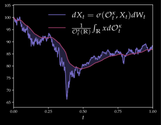
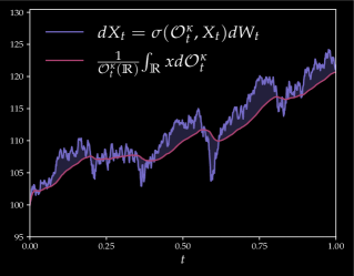
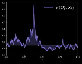
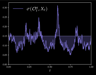
Example 10.

(Guyon’s toy volatility model) Consider the occupied volatility model,

$$\frac{1}{x}\sigma(o,x)=\Sigma(\Upsilon(o,x)),\quad\Sigma(y)=-\frac{\alpha}{\beta}+\gamma y^{-\beta},$$ (86)

with parameters $\alpha,\beta,\gamma>0$ and trend functional $\Upsilon$ defined in (83). Plugging in the exponential decay occupation measure (84) into (86), then the resulting specification $dX_{t}=\sigma(\operatorname{\mathcal{O}}^{\kappa}_{t},X_{t})dW_{t}$ is precisely Guyon’s toy volatility model, introduced in [37] and analyzed in [10]. As the function $\Sigma$ in (86) is decreasing, the volatility functional $\sigma$ is inversely proportional to the trend of the asset. This is in line with the leverage effect, a stylized fact in equity markets stating that volatility tends to increase when the asset price drops.

Fig. 9 displays two realizations of $(X,\sigma(\operatorname{\mathcal{O}}^{\kappa},X))$ where $X_{0}=100$, $T=1$ (in years), $\kappa=12$ (to reflect a one-month window for the weighted average (85)) and parameters $(\alpha,\beta,\gamma)=(2.1,1.2,1.9)$ taken from [37, page 25]. We indeed observe that the volatility shoots up when the asset falls far below the running average. The trajectories in Fig. 9 were simulated according to the Euler-Maruyama scheme in Section B.1 using $N=1,000$ time steps and levels $x_{m}=50+m$, $m=0,\ldots,100$.

6 Futher Work

We here gather some research areas where this work opens into.

Stochastic control and viscosity theory. We have seen in Theorem 3.4 a Feynman-Kac theorem linking Dirichlet problems to the solution of occupied stochastic differential equations (OSDEs). More generally, it would be relevant to introduce controlled OSDEs and, as hinted at by the optimal stopping problem in Section 4.1, to establish a viscosity theory for the associated dynamic programming equation as in [53, 54].

Itô-Tanaka’s formula. We proved in Theorem 3.1 the usual Itô’s formula where the occupation functional $f(o,x)$ is twice differentiable with respect to the space variable. It would be interesting to extend Itô-Tanaka’s formula [51, Chapter VI] (or more generally, Bouleau-Yor’s formula [12]) to our context, especially given the interplay between the occupation measure (or equivalently the local time) arising from the lack of regularity in $x$ and inside the functional itself.

Volatility Modeling. It would be worthwhile to further investigate occupied volatility models (Section 5.4) by incorporating other statistics of the occupation measure, e.g., the range of the asset which is available from the support of $\tilde{\operatorname{\mathcal{O}}}$ (or $\operatorname{\mathcal{O}}$). Alternatively, one could use neural SDEs as in [21, 40] where the occupied volatility is parameterized by a feedforward neural network, taking the (discretized) occupation measure and spot $X_{t}$ as input.

Appendix A Proofs

A.1 Theorem 2.1

Proof.

It is clear that II. $\Longrightarrow$ I. since the occupation measure is chronology invariant. Let us outline a proof for completeness. Fix $X\in\Lambda_{t}$, $\psi\in\operatorname{\mathfrak{S}}_{t}^{N}$ with permutation $\sigma$ and sign vector $\xi\in\{\pm 1\}^{N}$, and write $Y=X\circ\psi$. First, we may assume that $\xi_{n}=1$ for all $n$ as clearly $\tilde{\operatorname{\mathcal{O}}}(\overleftarrow{Z})=\tilde{\operatorname{\mathcal{O}}}(Z)$ for all $Z\in\Lambda$. From the additivity of $\tilde{\operatorname{\mathcal{O}}}$, we conclude that

$$\tilde{\operatorname{\mathcal{O}}}(Y)(A)=\sum_{n=1}^{N}\int_{I_{n}}\mathds{1}_{A}(Y_{s})ds=\sum_{n=1}^{N}\int_{I_{\sigma(n)}}\!\mathds{1}_{A}(X_{s})ds=\tilde{\operatorname{\mathcal{O}}}(X)(A),\quad\forall\ A\in\operatorname{\mathcal{B}}(\operatorname{\mathbb{R}}).$$

To prove I. $\Longrightarrow$ II. , introduce the equivalence relation $X\sim Y\ \Longleftrightarrow\ \tilde{\operatorname{\mathcal{O}}}(X)=\tilde{\operatorname{\mathcal{O}}}(Y)$ and construct a representative for the equivalence classes in $\Lambda/\!\sim$ by characterizing the pre-image of $\tilde{\operatorname{\mathcal{O}}}\mathrel{\mathop{\ordinarycolon}}\Lambda\to\operatorname{\mathcal{M}}$. Given $o=\tilde{\operatorname{\mathcal{O}}}(X)\in\operatorname{\mathcal{M}}$ for some $X\in\Lambda_{t}$, let $Z^{o}\in\Lambda_{t}$ defined as

$$Z_{s}^{o}=\sup\{x\in\operatorname{\mathbb{R}}\ \mathrel{\mathop{\ordinarycolon}}\ o((-\infty,x])\leq s\},\quad s\leq t.$$ (87)

Since $Z^{o}_{s}\leq x\ \Longleftrightarrow\ o((-\infty,x])\geq s$ by construction, it is then immediate that $\tilde{\operatorname{\mathcal{O}}}(Z^{o})=o$. Moreover, $Z^{o}$ is clearly càdlàg and non-decreasing. See Fig. 10. We can therefore define the representation map $\operatorname{\mathcal{R}}\mathrel{\mathop{\ordinarycolon}}\operatorname{\mathcal{M}}\to\Lambda_{t}/\!\sim$, $\operatorname{\mathcal{R}}(o)=Z^{o}$ and projection $\pi\mathrel{\mathop{\ordinarycolon}}\Lambda_{t}\to\Lambda_{t}/\!\sim$ as $\pi=\operatorname{\mathcal{R}}\circ\ \tilde{\operatorname{\mathcal{O}}}$. In short,

$$X\ \mapsto\ \tilde{\operatorname{\mathcal{O}}}_{t}=\tilde{\operatorname{\mathcal{O}}}(X)\ \mapsto\ \operatorname{\mathcal{R}}(\tilde{\operatorname{\mathcal{O}}}_{t})=Z^{\tilde{\operatorname{\mathcal{O}}}_{t}}\in\Lambda_{t}/\!\sim.$$

Next, fix a chronology-invariant functional $F\mathrel{\mathop{\ordinarycolon}}\Lambda\to\operatorname{\mathbb{R}}$ and $X\in\Lambda_{t}$. If $X$ is constant in each subinterval of the partition $\{\frac{nt}{N}\mathrel{\mathop{\ordinarycolon}}n\leq N\}$ for some $N\in\operatorname{\mathbb{N}}$, then $\tilde{\operatorname{\mathcal{O}}}_{t}=\tilde{\operatorname{\mathcal{O}}}(X)$ is a discrete measure so the representative $Z^{\tilde{\operatorname{\mathcal{O}}}_{t}}$ is piecewise constant as well. Thus, there exists a ”sorting” permutation $\psi\in\operatorname{\mathfrak{S}}_{t}^{N}$ such that $X\circ\psi$ is non-decreasing and as $\operatorname{\mathcal{O}}(X\circ\psi)=\operatorname{\mathcal{O}}_{t}$, we gather that $Z^{\tilde{\operatorname{\mathcal{O}}}_{t}}=X\circ\psi$. For general càdlàg $X$, the same reasoning can be applied by first taking a piecewise constant approximation of $X$ as seen in Section 2.3 and a passage to the limit. To conclude, set $f\mathrel{\mathop{\ordinarycolon}}=F\circ\operatorname{\mathcal{R}}\mathrel{\mathop{\ordinarycolon}}\operatorname{\mathcal{M}}\to\operatorname{\mathbb{R}}$ and $\psi\in\operatorname{\mathfrak{S}}_{t}$ such that $Z^{\tilde{\operatorname{\mathcal{O}}}_{t}}=X\circ\psi$. Hence,

$$(f\circ\tilde{\operatorname{\mathcal{O}}})(X)=f(\tilde{\operatorname{\mathcal{O}}}_{t})=(F\circ\operatorname{\mathcal{R}})(\tilde{\operatorname{\mathcal{O}}}_{t})=F(Z^{\tilde{\operatorname{\mathcal{O}}}_{t}})=F(X\circ\psi)=F(X).$$

∎

Figure 10: Path $X\in\Lambda_{t}$, its standard time occupation measure $\tilde{\operatorname{\mathcal{O}}}_{t}$, and representative path $Z_{t}^{\tilde{\operatorname{\mathcal{O}}}_{t}}$ in the proof of Theorem 2.1. Two simulations.

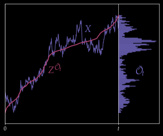
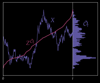
A.2 Theorem 3.1

Proof.

Let $\Pi^{N}=\{s=t_{0}<...<t_{N}=t\}$ be a sequence of partitions with mesh size decreasing to zero as $N\to\infty$. If $f\in\operatorname{\mathcal{C}}^{1,2}(\operatorname{\mathcal{D}})$ and $Y_{t}=f(\operatorname{\mathcal{O}}_{t},X_{t})$, then,

$$Y_{t}-Y_{s} =\sum_{t_{n}\in\Pi^{N}}(Y_{t_{n+1}}-Y_{t_{n}})\quad\qquad(t_{N+1}\mathrel{\mathop{\ordinarycolon}}=t)$$

$$=\sum_{t_{n}\in\Pi^{N}}(Y_{t_{n+1}}-f(\operatorname{\mathcal{O}}_{t_{n}},X_{t_{n+1}}))$$ (88)

$$+\sum_{t_{n}\in\Pi^{N}}(f(\operatorname{\mathcal{O}}_{t_{n}},X_{t_{n+1}})-Y_{t_{n}})$$ (89)

The telescopic sum (89) generates the terms $\int_{s}^{t}\partial_{x}f(\operatorname{\mathcal{O}}_{u},X_{u})dX_{u}$ and $\int_{s}^{t}\frac{1}{2}\partial_{xx}f(\operatorname{\mathcal{O}}_{u},X_{u})d\langle X\rangle_{u}$ (for $\operatorname{\mathbb{Q}}-$almost all $\omega\in\Omega$ and a suitable sequence $(\Pi^{N})$) as the occupation measure appearing in the summand of (89) is ”frozen” at time $t_{n}$ for each $n$. Concretely, defining the predictable processes $H^{(1)}_{t}=\partial_{x}f(\operatorname{\mathcal{O}}_{t},X_{t})$, $H_{t}^{(2)}=\partial_{xx}f(\operatorname{\mathcal{O}}_{t},X_{t})$, a second order Taylor expansion in the space variable yields

$$\sum_{t_{n}\in\Pi^{N}}(f(\operatorname{\mathcal{O}}_{t_{n}},X_{t_{n+1}})-Y_{t_{n}})=\sum_{t_{n}\in\Pi^{N}}H_{t_{n}}^{(1)}(X_{t_{n+1}}-X_{t_{n}})+\frac{1}{2}\sum_{t_{n}\in\Pi^{N}}H_{t_{n}}^{(2)}(X_{t_{n+1}}-X_{t_{n}})^{2}+o(1),$$

so the result follows from the standard Itô’s formula. We now compute the limit of (88) as $N\to\infty$. In light of the definition of $\delta_{\mu}$ (Definition 2), we set $\Delta_{n}=\operatorname{\mathcal{O}}_{t_{n},t_{n+1}}=\operatorname{\mathcal{O}}_{t_{n+1}}-\operatorname{\mathcal{O}}_{t_{n}}$ for simplicity (note that $\Delta_{n}$ depends on $N$) and rewrite the summands in (88) as

$$Y_{t_{n+1}}-f(\operatorname{\mathcal{O}}_{t_{n}},X_{t_{n+1}})=\int_{0}^{1}\delta_{\mu}f(\operatorname{\mathcal{O}}_{t_{n}}+\eta\Delta_{n},X_{t_{n+1}})\cdot\Delta_{n}d\eta=\delta_{\mu}f(\operatorname{\mathcal{O}}_{t_{n}}+\eta_{n}\Delta_{n},X_{t_{n+1}})\cdot\Delta_{n},$$

for some $\eta_{n}\in[0,1]$ by the mean value theorem. Next, the occupation time formula (10) yields

$$\sum_{t_{n}\in\Pi^{N}}(Y_{t_{n+1}}-f(\operatorname{\mathcal{O}}_{t_{n}},X_{t_{n+1}})) =\sum_{t_{n}\in\Pi^{N}}\delta_{\mu}f(\operatorname{\mathcal{O}}_{t_{n}}+\eta_{n}\Delta_{n},X_{t_{n+1}})\cdot\Delta_{n}$$

$$=\sum_{t_{n}\in\Pi^{N}}\int_{t_{n}}^{t_{n+1}}\delta_{\mu}f(\operatorname{\mathcal{O}}_{t_{n}}+\eta_{n}\Delta_{n},X_{t_{n+1}})(X_{u})d\langle X\rangle_{u}$$

$$=\int_{s}^{t}Z^{N}_{u}d\langle X\rangle_{u},$$

with the step process

$$Z^{N}_{u}=\sum_{t_{n}\in\Pi^{N}}\delta_{\mu}f(\operatorname{\mathcal{O}}_{t_{n}}+\eta_{n}\Delta_{n},X_{t_{n+1}})(X_{u})\ \mathds{1}_{[t_{n},t_{n}+1)}(u),\qquad[t_{N},t_{N+1})=\{t\}.$$

For every $n$ and $u\in[t_{n},t_{n+1})$, observe that $\operatorname{\mathfrak{m}}_{1}(\operatorname{\mathcal{O}}_{u},\operatorname{\mathcal{O}}_{t_{n}}+\eta_{n}\Delta_{n})=\eta_{n}\Delta_{n}(\operatorname{\mathbb{R}})\leq\frac{T}{N}$ and $|X_{u}-X_{t_{n+1}}|\leq\rho(\frac{T}{N})$, where $\rho=\rho(\omega)$ is the modulus of continuity of $t\mapsto X_{t}$ on the compact $[s,t]$. As $(o,x,y)\mapsto\delta_{\mu}f(o,x)(y)$ is jointly continuous, we have

$$Z^{N}_{u}\to Z_{u}^{\infty}=\delta_{\mu}f(\operatorname{\mathcal{O}}_{u},X_{u})(X_{u})=\partial_{o}f(\operatorname{\mathcal{O}}_{u},X_{u}),$$

uniformly in $u\in[s,t]$, $\operatorname{\mathbb{Q}}-$almost surely. We finally conclude that

$$\lim_{N\to\infty}\int_{s}^{t}Z^{N}_{u}d\langle X\rangle_{u}=\int_{s}^{t}\partial_{o}f(\operatorname{\mathcal{O}}_{u},X_{u})d\langle X\rangle_{u},\quad\operatorname{\mathbb{Q}}-a.s.$$

∎

A.3 Proposition 4

Proof.

First, the additivity property of the occupation measure gives

$$\operatorname{\mathcal{O}}(X+h\mathds{1}_{[t,T]})(A)=\operatorname{\mathcal{O}}_{t}(A)+\int_{t}^{T}\mathds{1}_{A}(X_{s}+h)ds=\operatorname{\mathcal{O}}_{t}(A)+\operatorname{\mathcal{O}}_{t,T}^{h}(A),\quad\forall A\in\operatorname{\mathcal{B}}(\operatorname{\mathbb{R}}),$$

where $\operatorname{\mathcal{O}}^{h}(A)=\operatorname{\mathcal{O}}(A-h)$. Hence, a parallel shift of $X$ in $[t,T]$ induces a translation of the increment occupation measure $\operatorname{\mathcal{O}}_{t,T}$. Writing $\Delta_{t,T}^{h}=\operatorname{\mathcal{O}}_{t,T}^{h}-\operatorname{\mathcal{O}}_{t,T}$, then from the definition of $\delta_{\mu}$ and $F$, we have

$$F(X+h\mathds{1}_{[t,T]})-F(X) =\int_{0}^{1}\delta_{\mu}f(\operatorname{\mathcal{O}}_{T}+\eta\Delta_{T}^{t,h})\cdot\Delta_{t,T}^{h}\ d\eta=\delta_{\mu}f(\operatorname{\mathcal{O}}_{T}+\eta^{h}\Delta_{T}^{t,h})\cdot\Delta_{t,T}^{h},$$

for some $\eta^{h}\in[0,1]$. Formally, $\lim\limits_{h\to 0}\frac{\Delta_{t,T}^{h}(A)}{h}=\lim\limits_{h\to 0}\int_{A}\frac{L^{x-h}_{t,T}-L^{x}_{t,T}}{h}dx=-\int_{A}\partial_{x}L_{t,T}^{x}dx,$ hence

$$D_{t}f(\operatorname{\mathcal{O}}_{T})=-\int_{\operatorname{\mathbb{R}}}\delta_{\mu}f(\operatorname{\mathcal{O}}_{T})(x)\partial_{x}L_{t,T}^{x}dx=\int_{\operatorname{\mathbb{R}}}\partial_{xo}f(\operatorname{\mathcal{O}}_{T},x)L_{t,T}^{x}dx=\int_{t}^{T}\partial_{xo}f(\operatorname{\mathcal{O}}_{T},X_{u})du,$$

using integration by parts and the occupation time formula. Although local time of Brownian motion is $\operatorname{\mathbb{Q}}-$a.s. nowhere differentiable (e.g. as a consequence of the first Ray-Knight theorem [51, Chapter XI]), this instructive heuristics turns out to be correct. Indeed, for all $\phi\in\operatorname{\mathcal{C}}^{1}(\operatorname{\mathbb{R}})$, we have using the occupation time formula that

$$\frac{1}{h}(\phi\cdot\Delta_{t,T}^{h})=\frac{1}{h}\int_{t}^{T}\phi(X_{s}+h)ds\longrightarrow\int_{t}^{T}\partial_{x}\phi(X_{s})ds.$$

Noting that $\delta_{\mu}f(\operatorname{\mathcal{O}}_{T}+\eta^{h}\Delta_{t,T}^{h})=\delta_{\mu}f(\operatorname{\mathcal{O}}_{T})+\varepsilon_{h}$, $\lim_{h\to 0}\varepsilon_{h}=0$, we can apply the above limit to $\phi=\delta_{\mu}f(\operatorname{\mathcal{O}}_{T})\in\operatorname{\mathcal{C}}^{1}(\operatorname{\mathbb{R}})$ and obtain (41). ∎

A.4 Theorem 3.2

Proof.

The first assertion follows from the fact that $v(\operatorname{\mathcal{O}},X)$ is an $(\operatorname{\mathbb{F}},\operatorname{\mathbb{Q}})-$martingale, as a consequence of (42a) and Itô’s formula (Theorem 3.1) applied to $v\in\operatorname{\mathcal{C}}^{1,2}(\operatorname{\mathcal{D}})$. Hence $v(o,x)=\operatorname{\mathbb{E}}_{o,x}^{\operatorname{\mathbb{Q}}}[v(\operatorname{\mathcal{O}}_{T},X_{T})]$, which is (43) in light of the terminal condition (42b).

For the second part, it is enough to verify that $v\in\operatorname{\mathcal{C}}^{2}_{2}(\operatorname{\mathcal{D}})$ as the uniqueness then follows from the previous assertion. For all $o,o^{\prime}\in\operatorname{\mathcal{M}}$, $\Delta=o^{\prime}-o$, and condition (25), observe that

$$v(o^{\prime},x)-v(o,x) =\operatorname{\mathbb{E}}^{\operatorname{\mathbb{Q}}}[\varphi(o^{\prime}+\operatorname{\mathcal{O}}_{T-t}^{x},x+X_{T-t})-\varphi(o+\operatorname{\mathcal{O}}_{T-t}^{x},x+X_{T-t})]$$

$$=\operatorname{\mathbb{E}}^{\operatorname{\mathbb{Q}}}\left[\int_{0}^{1}\delta_{\mu}\varphi(o+\operatorname{\mathcal{O}}_{T-t}^{x}+\eta\Delta,x+X_{T-t})\cdot\Delta\ d\eta\right]$$

$$=\int_{0}^{1}w(o+\eta\Delta,x,\cdot)\cdot\Delta\ d\eta,$$

$$w(o,x,y) =\operatorname{\mathbb{E}}^{\operatorname{\mathbb{Q}}}[\delta_{\mu}\varphi(o+\operatorname{\mathcal{O}}_{T-t}^{x},x+X_{T-t})(y)].$$

Clearly, the joint continuity of $(o,x,y)\mapsto\delta_{\mu}\varphi(o,x)(y)$ carries over to $w$. Moreover, defining $C\mathrel{\mathop{\ordinarycolon}}=\sup_{(o,x)\in\operatorname{\mathcal{D}},y\in\operatorname{\mathbb{R}}}\frac{|\delta_{\mu}\varphi(o,x)(y)|}{1+|y|^{2}}$ which is finite as $\varphi\in\operatorname{\mathcal{C}}_{2}^{2}(\operatorname{\mathcal{D}})$, we have from Jensen’s inequality that $|w(o,x,y)|\leq C(1+|y|^{2})$, uniformly in $(o,x)$. Hence $\delta_{\mu}v=w$ in light of Definition 2, which implies that $v\in\operatorname{\mathcal{C}}^{1,0}(\operatorname{\mathcal{D}})$. Next, it is easily seen that

$$\delta_{\mu\mu}v(o,x)(y,y^{\prime})=\delta_{\mu}w(o,x,y)(y^{\prime})=\operatorname{\mathbb{E}}^{\operatorname{\mathbb{Q}}}[\delta_{\mu\mu}\varphi(o+\operatorname{\mathcal{O}}_{T-t}^{x},x+X_{T-t})(y,y^{\prime})],$$

which is, similar to $\varphi$, continuous in $(o,x)$, twice differentiable with respect to $(y,y^{\prime})$ and satisfies the quadratic growth condition II. in Definition 2 (with respect to $y^{\prime}$).

Moving to the space derivatives, observe that for every $f\in\operatorname{\mathcal{C}}^{1}(\operatorname{\mathcal{M}})$ such that $y\mapsto\delta_{\mu}f(o)(y)\in\operatorname{\mathcal{C}}^{1}(\operatorname{\mathbb{R}})$, we have $\frac{d}{dh}f(o+\operatorname{\mathcal{O}}_{s}^{x+h})=\partial_{y}\delta_{\mu}f(o+\operatorname{\mathcal{O}}_{s}^{x})\cdot\operatorname{\mathcal{O}}_{s}^{x}$ using similar arguments as in the proof of Proposition 4; see Section A.3. Thus, the chain rule and bounded convergence theorem yields

$$\partial_{x}v(o,x) =\underbrace{\operatorname{\mathbb{E}}^{\operatorname{\mathbb{Q}}}[\partial_{x}\varphi(o+\operatorname{\mathcal{O}}_{T-t}^{x},x+X_{T-t})]}_{=\mathrel{\mathop{\ordinarycolon}}\ w_{1}^{\varphi}(o,x)}+\underbrace{\operatorname{\mathbb{E}}^{\operatorname{\mathbb{Q}}}[\partial_{y}\delta_{\mu}\varphi(o+\operatorname{\mathcal{O}}_{T-t}^{x},x+X_{T-t})\cdot\operatorname{\mathcal{O}}_{T-t}^{x}]}_{=\mathrel{\mathop{\ordinarycolon}}\ w_{2}^{\varphi}(o,x)},$$

which is jointly continuous. Next, it is immediate that $\partial_{x}w_{1}^{\varphi}=w_{1}^{\partial_{x}\varphi}+w_{2}^{\partial_{x}\varphi}\in\operatorname{\mathcal{C}}(\operatorname{\mathcal{D}})$. For $w_{2}^{\varphi}$, we compute

$$\partial_{x}w_{2}^{\varphi}(o,x) =\operatorname{\mathbb{E}}^{\operatorname{\mathbb{Q}}}[(\partial_{x}+\partial_{y})\partial_{y}\delta_{\mu}\varphi(o+\operatorname{\mathcal{O}}_{T-t}^{x},x+X_{T-t})\cdot\operatorname{\mathcal{O}}_{T-t}^{x}],$$

$$+\operatorname{\mathbb{E}}^{\operatorname{\mathbb{Q}}}[\partial_{y^{\prime}y}\delta_{\mu\mu}(o+\operatorname{\mathcal{O}}_{T-t}^{x},x+X_{T-t})\cdot(\operatorname{\mathcal{O}}_{T-t}^{x}\otimes\operatorname{\mathcal{O}}_{T-t}^{x})]$$

where $\phi\cdot(o\otimes o^{\prime})=\int_{\operatorname{\mathbb{R}}^{2}}\phi(y,y^{\prime})o(dy)o^{\prime}(dy^{\prime})$, $\phi\mathrel{\mathop{\ordinarycolon}}\operatorname{\mathbb{R}}^{2}\to\operatorname{\mathbb{R}}$, and using [15, Lemma 2.2.4.] to rewrite $\partial_{y^{\prime}}\delta_{\mu}\partial_{y}\delta_{\mu}$ more compactly as $\partial_{y^{\prime}y}\delta_{\mu\mu}$. Given our assumptions on $\varphi$, we conclude that $\partial_{x}w_{2}^{\varphi}\in\operatorname{\mathcal{C}}(\operatorname{\mathcal{D}})$ and thus $v\in\operatorname{\mathcal{C}}^{2}_{2}(\operatorname{\mathcal{D}})$. ∎

A.5 Proposition 6

Proof.

Let $\overleftarrow{X}_{s}=X_{T-s}-X_{T}$ and denote its flow of occupation measures by $\overleftarrow{\operatorname{\mathcal{O}}}$ and local time field by $\overleftarrow{L}$. Then, $L_{T}^{X_{T}+z}=\overleftarrow{L_{T}^{z}}$ for all $z\in\operatorname{\mathbb{R}}$, which implies that

$$\varphi^{\varepsilon}(\operatorname{\mathcal{O}}_{T},X_{T})=\mathop{\,\,\hbox to0.0pt{--\hss}\int}\nolimits_{B_{\varepsilon}}L_{T}^{X_{T}+z}dz=\mathop{\,\,\hbox to0.0pt{--\hss}\int}\nolimits_{B_{\varepsilon}}\overleftarrow{L_{T}}\ d\lambda=\varphi^{\varepsilon}(\overleftarrow{\operatorname{\mathcal{O}}}_{T},0).$$

Thus,

$$v^{\varepsilon}(T) =\operatorname{\mathbb{E}}^{\operatorname{\mathbb{Q}}}[\varphi^{\varepsilon}(\overleftarrow{\operatorname{\mathcal{O}}}_{T},0)]=\mathop{\,\,\hbox to0.0pt{--\hss}\int}\nolimits_{B_{\varepsilon}}\operatorname{\mathbb{E}}^{\operatorname{\mathbb{Q}}}[\overleftarrow{L}_{T}]d\lambda=\mathop{\,\,\hbox to0.0pt{--\hss}\int}\nolimits_{[0,\varepsilon]}\operatorname{\mathbb{E}}^{\operatorname{\mathbb{Q}}}[L_{T}^{x}]dx\ \uparrow\ \operatorname{\mathbb{E}}^{\operatorname{\mathbb{Q}}}[L_{T}^{0}],$$

where we used that $\text{Law}_{\operatorname{\mathbb{Q}}}(\overleftarrow{L}_{T}^{x})=\text{Law}_{\operatorname{\mathbb{Q}}}(L_{T}^{x})$ and $\partial_{x}\operatorname{\mathbb{E}}^{\operatorname{\mathbb{Q}}}[L_{T}^{x}]<0$ $\forall x>0$ to prove the monotone convergence. Finally, recall from Proposition 5 that $\operatorname{\mathbb{E}}^{\operatorname{\mathbb{Q}}}[L_{T}^{0}]=v(T)$. For the second assertion, notice from Tanaka’s formula that $\operatorname{\mathbb{E}}^{\operatorname{\mathbb{Q}}}[L_{T}^{x}]=2c(T,x)$, where $c(T,x)=\operatorname{\mathbb{E}}^{\operatorname{\mathbb{Q}}}[(X_{T}-x)^{+}]$ is the price of a call option struck at $x$ with maturity $T$ in a Bachelier model with unit volatility. Similar to [14], we have $\partial_{x}c(T,x)=\operatorname{\mathbb{Q}}(X_{T}\leq x)-1=\Phi_{T}(x)-1$ and $\partial_{xx}c(T,x)=\phi_{T}(x)$, where $\Phi_{T},\phi_{T}$ is the CDF and PDF of $\operatorname{\mathcal{N}}(0,T)$, respectively. Hence, a second order Taylor expansion of $x\mapsto c(T,x)$ at $x=0$ yields

$$v^{\varepsilon}(T)=\frac{2}{\varepsilon}\int_{0}^{\varepsilon}c(T,x)dx=v(T)-\frac{\varepsilon}{2}+\frac{\varepsilon^{2}/3}{\sqrt{2\pi T}}(1+r_{\varepsilon}),\quad\lim_{\varepsilon\downarrow 0}r_{\varepsilon}=0.$$

∎

A.6 Proposition 7

Proof.

For every stopping time $\tau\in\vartheta(\operatorname{\mathcal{T}})$, $x\in\operatorname{\mathbb{R}}$, we have by Jensen’s inequality that

$$|\varphi^{\varepsilon}(\operatorname{\mathcal{O}}_{\tau},x)-L_{\tau}^{x}|^{2}=\left|\mathop{\,\,\hbox to0.0pt{--\hss}\int}\nolimits_{B_{\varepsilon}}(L_{\tau}^{x+z}-L_{\tau}^{x})\ dz\right|^{2}\leq\mathop{\,\,\hbox to0.0pt{--\hss}\int}\nolimits_{B_{\varepsilon}}|L_{\tau}^{x+z}-L_{\tau}^{x}|^{2}\ dz.$$

Moreover, there exists $C>0$ (to be determined) such that

$$\left\lVert\sup_{(t,x)\in[0,T]\times\operatorname{\mathbb{R}}}|L_{t}^{x+z}-L_{t}^{x}|\right\rVert_{L^{2}(\operatorname{\mathbb{Q}})}^{2}\leq C|z|,\quad|z|\leq 1.$$

Indeed, writing $L^{x}(Y)$ for the local time of some process $Y$ at $x$ and ${|\!|\!|Y|\!|\!|}\mathrel{\mathop{\ordinarycolon}}=\lVert\sup_{t\in[0,T]}Y_{t}\rVert_{L^{2}(\operatorname{\mathbb{Q}})}$, we can apply Theorem 6.5 in Barlow and Yor [2] with $\gamma=2$ to the continuous martingales $M=X-z$, $N=X$. This yields

$$\left\lVert\sup_{(t,x)\in[0,T]\times\operatorname{\mathbb{R}}}|L_{t}^{x+z}-L_{t}^{x}|\right\rVert_{L^{2}(\operatorname{\mathbb{Q}})}^{2} =\left\lVert\sup_{(t,x)\in[0,T]\times\operatorname{\mathbb{R}}}|L_{t}^{x}(M)-L_{t}^{x}(N)|\right\rVert_{L^{2}(\operatorname{\mathbb{Q}})}^{2}$$

$$\leq C_{2}^{2}\ ({|\!|\!|M|\!|\!|}+{|\!|\!|N|\!|\!|})\underbrace{{|\!|\!|M-N|\!|\!|}}_{=\ |z|}\ \max\left(\log\frac{{|\!|\!|M|\!|\!|}+{|\!|\!|N|\!|\!|}}{{|\!|\!|M-N|\!|\!|}},1\right)$$

$$\leq 2C|z|,$$

with $C=C_{2}^{2}\ \sqrt{2(T+1)}\max(\log 2\sqrt{2(T+1)}/|z|,1)$ and $C_{2}$ as in [2, Theorem 6.5]. Thus,

$$\left\lVert\varphi^{\varepsilon}(X_{\tau},\operatorname{\mathcal{O}}_{\tau})-L_{\tau}^{X_{\tau}}\right\rVert_{L^{2}(\operatorname{\mathbb{Q}})}^{2} \leq\mathop{\,\,\hbox to0.0pt{--\hss}\int}\nolimits_{B_{\varepsilon}}\left\lVert L_{\tau}^{X_{\tau}+z}-L_{\tau}^{X_{\tau}}\right\rVert_{L^{2}(\operatorname{\mathbb{Q}})}^{2}\ dz\leq 2C\mathop{\,\,\hbox to0.0pt{--\hss}\int}\nolimits_{B_{\varepsilon}}|z|dz=C\varepsilon,\quad\forall\ \varepsilon\leq 1.$$

The second assertion simply follows from Jensen’s inequality. ∎

Appendix B Algorithms

B.1 Numerical Integration of OSDEs

This section provides practical details towards the simulation of processes $X$ governed by OSDEs, that is $dX_{t}=b(\operatorname{\mathcal{O}}_{t},X_{t})dt+\sigma(\operatorname{\mathcal{O}}_{t},X_{t})dW_{t},$ $X_{0}\in\operatorname{\mathbb{R}}$, and $\operatorname{\mathcal{O}}$ evolving as in (46b). An almost identical procedure can be carried out for OSDEs depending on the standard time or exponential decay occupation measure as in Example 10.

First, fix $N\in\operatorname{\mathbb{N}}$ and the regular time partition $t_{n}=n\delta t$, $\delta t=\frac{T}{N}$. To make the simulation procedure feasible, the occupation measure must be inevitably discretized. Let $x_{1}<\ldots<x_{M}$, $M\in\operatorname{\mathbb{N}}$, be prescribed levels and consider the partition

$$C^{m}=[x_{m}-\varepsilon_{m-1},x_{m}+\varepsilon_{m}),\quad\varepsilon_{m}=\frac{x_{m+1}-x_{m}}{2},\quad(x_{M+1}=-x_{0}=\infty).$$

The choice for $x_{1}<\ldots<x_{M}$ is natural once the initial value $X_{0}$ and scale of the coefficients $b,\sigma$ are set; see Example 10. Next, define the discrete occupation measure,

$$\operatorname{\mathcal{O}}_{t_{n}}^{M}=\sum_{m=1}^{M}\operatorname{\mathcal{O}}_{t_{n}}(C_{m})\delta_{x_{m}},$$

which is in one-to-one correspondence with $O_{t_{n}}\mathrel{\mathop{\ordinarycolon}}=(O^{1}_{t_{n}},\ldots,O^{M}_{t_{n}})\in\operatorname{\mathbb{R}}^{M}$, $O^{m}_{t}=\operatorname{\mathcal{O}}_{t}(C_{m})$. We can then introduce the function $b^{M}\mathrel{\mathop{\ordinarycolon}}\operatorname{\mathbb{R}}^{M}\times\operatorname{\mathbb{R}}\to\operatorname{\mathbb{R}}$, $b^{M}(O_{t},X_{t})=b(\operatorname{\mathcal{O}}_{t}^{M},X_{t})$, and similarly for $\sigma^{M}$.

If $X_{0}\in\operatorname{\mathbb{R}}$, $O^{\text{\tiny tmp}}=0\in\operatorname{\mathbb{R}}^{M}$, and $e_{m}$ is the $m$-th row of the $M\times M$ identity matrix, we can approximate the solution of (46a)$-$(46b) according to the Euler-Maruyama scheme (see, e.g., [43]),

$$X_{t_{n}}\! X_{t_{n-1}}+b^{M}(O^{\text{\tiny tmp}},X_{t_{n-1}})\delta t+\sigma^{M}(O^{\text{\tiny tmp}},X_{t_{n-1}})\sqrt{\delta t}Z_{n},$$ =   (90a)

$$O^{\text{\tiny tmp}}\! \leftarrow\ O^{\text{\tiny tmp}}+e_{m}\sigma^{M}(O^{\text{\tiny tmp}},X_{t_{n}})^{2}\delta t,\quad X_{t_{n}}\ \in\ C_{m}$$ , (90b)

where $Z_{n}\overset{i.i.d.}{\sim}\operatorname{\mathcal{N}}(0,1)$, $n=1,\ldots,N$. For OSDEs entailing the standard time occupation measure, then (90b) is replaced by $O^{\text{\tiny tmp}}\leftarrow O^{\text{\tiny tmp}}+e_{m}\delta t$. Note that the occupation measure is represented by the temporary variable $O^{\text{\tiny tmp}}$ updated at each iteration. Indeed, it is not necessary (and costly) to store the occupation measure $\tilde{\operatorname{\mathcal{O}}}_{t_{n}}$ for each $n$. If one is interested in the flow $\operatorname{\mathcal{O}}$, it can be retrieved from the simulated path anyway.

Note that for fully path-dependent SDEs $dX_{t}=b((X_{s})_{s\leq t})dt+\sigma((X_{s})_{s\leq t})dW_{t},$ one has to store all the values so far $X_{t_{1}},\ldots,X_{t_{n}}$ to generate the next one. This becomes highly problematic when the time grid gets finer. In the case of OSDEs, we can, in contrast, decouple the dimensionality of the space and time discretization. Hence, the number of levels to approximate $\operatorname{\mathcal{O}}$ ($M$) can be set to fairly large values as demonstrated in Example 10.

B.2 Least Square Monte Carlo for Spot Local Time

Algorithm 1 summarizes the Least Square Monte Carlo approach seen in Section 4.3. Notice the exponential transformation of the discrete Brownian in step IV.2. so that all variables are nonnegative. We choose a family of functions on $\operatorname{\mathbb{R}}_{+}$, namely the Laguerre polynomials $(p_{k})$ (up to degree $3$) which are orthonormal in the weighted Hilbert space $L^{2}(\operatorname{\mathbb{R}}_{+},wd\lambda)$, $w(x)=e^{-x}$. The basis functions $\phi_{k}$ in Algorithm 1 then corresponds to individual evaluations of the feature variables $\operatorname{\mathcal{O}}_{t_{n}}^{\bar{m}},\bar{X}_{t_{n}}$ through the polynomials. Note that $p_{1}(\operatorname{\mathcal{O}}_{t_{n}}^{\bar{m}})\mathrel{\mathop{\ordinarycolon}}=(p_{1}(L_{t_{n}}^{x_{m-\bar{m}}}),\ldots,p_{1}(L_{t_{n}}^{x_{m+\bar{m}}}))$ contains the intrinsic value $L_{t_{n}}^{X_{t_{n}}}$ itself (up to a constant) which is of course valuable information. One can also choose instead, as in [48], the better-behaved Laguerre polynomials weighted by $\sqrt{w}$, yielding similar results.

In both phases, we use antithetic sampling, i.e., we simulate $X(\omega_{j})$ for $j=1,\ldots,J/2$ (provided that $J$ is even) and set $X(\omega_{j})=-X(\omega_{j-J/2})$ for $j=J/2+1,\ldots,J$, $J\in\{J_{\text{off}},J_{\text{on}}\}$.

Algorithm 1 (Least Square Monte Carlo, Spot Local Time)

$T>0$, $N\in\operatorname{\mathbb{N}}$, $\bar{m}\ll N$ (truncation level), $J_{\text{off}}$ (# simulations, offline phase), $J_{\text{on}}$ (# simulations, online phase), $\{\phi_{k}\mathrel{\mathop{\ordinarycolon}}k=1,\ldots,K\}$ (basis functions)
  OFFLINE

• Space-time grid $\begin{cases}t_{n}\ =n\delta t,\;\ &n=0,\ldots,N,\quad\delta t=\frac{T}{N},\\ x_{m}=m\sqrt{3\delta t},\;\ &m=-N,\ldots,N\end{cases}$

• Generate paths $X(\omega_{j})$, $j=1,\ldots,J_{\text{off}}$, where

  $$X_{t_{n+1}}=X_{t_{n}}+Z_{n+1}\sqrt{\delta t},\quad X_{0}=0,\quad Z_{1},\ldots,Z_{N}\overset{i.i.d.}{\sim}\nu=\frac{1}{6}\left(\delta_{-\sqrt{3}}+4\delta_{0}+\delta_{\sqrt{3}}\right)$$

• Terminal value $Y_{T}=L_{T}^{X_{T}}=\frac{1}{2\varepsilon}\sum_{n=1}^{N}\mathds{1}_{\{X_{t_{n}}=X_{T}\}}\delta t$, $\ \varepsilon=\frac{x_{m+1}-x_{m}}{2}=\frac{\sqrt{3\delta t}}{2}$.

• For $n=N-1,\ldots,\bar{m}$:

  1. Let $\operatorname{\mathcal{J}}=\{j=1,\ldots,J_{\text{off}}\ \mathrel{\mathop{\ordinarycolon}}\ X_{t_{n}}(\omega_{j})=x_{m},\ |m|\leq n-\bar{m}\}$

  2. Feature variables: $\bar{X}_{t_{n}}=e^{X_{t_{n}}}$, $\operatorname{\mathcal{O}}_{t_{n}}^{\bar{m}}=(L_{t_{n}}^{x_{m-\bar{m}}},\ldots,L_{t_{n}}^{x_{m+\bar{m}}})$, $x_{m}=X_{t_{n}}$.

  3. Regression: $\hat{\beta}^{n}=\text{argmin}_{\beta}\sum_{j\in\operatorname{\mathcal{J}}}\left|Y_{t_{n+1}}-\sum_{k=1}^{K}\beta_{k}\ \phi_{k}(\operatorname{\mathcal{O}}_{t_{n}}^{\bar{m}},\bar{X}_{t_{n}})\right|^{2}(\omega_{j})$.

  4. Continuation value: $C_{t_{n}}=\sum_{k=1}^{K}\hat{\beta}_{k}^{n}\ \phi_{k}(\operatorname{\mathcal{O}}_{t_{n}}^{\bar{m}},\bar{X}_{t_{n}})$.

  5. Update: $Y_{t_{n}}(\omega_{j})=\begin{cases}Y_{t_{n+1}}(\omega_{j}),&C_{t_{n}}(\omega_{j})>L_{t_{n}}^{X_{t_{n}}}(\omega_{j})\text{ or }j\notin\operatorname{\mathcal{J}},\\ L_{t_{n}}^{X_{t_{n}}}(\omega_{j}),&\text{otherwise}.\end{cases}$

ONLINE

• Generate paths $X(\omega_{j})$, $j=1,\ldots,J_{\text{on}}$ as in II.

• Repeat steps III., IV.1, 2, 4, 5 using $\hat{\beta}^{N-1},\ldots,\hat{\beta}^{\bar{m}}$ from IV.3.

• Return $Y_{0}=\frac{1}{J_{\text{on}}}\sum_{j=1}^{J_{\text{on}}}Y_{t_{1}}(\omega_{j})$.

References

- Arous [1989] G. B. Arous. Flots et séries de Taylor stochastiques. Probability Theory and Related Fields, 81:29–77, 1989.
- Barlow and Yor [1982] M. Barlow and M. Yor. Semi-martingale inequalities via the Garsia-Rodemich-Rumsey lemma, and applications to local times. Journal of Functional Analysis, 49(2):198–229, 1982.
- Bayer et al. [2023] C. Bayer, P. P. Hager, S. Riedel, and J. Schoenmakers. Optimal stopping with signatures. The Annals of Applied Probability, 33(1):238 – 273, 2023.
- Bayraktar et al. [2023] E. Bayraktar, Q. Feng, and Z. Zhang. Deep signature algorithm for multi-dimensional path-dependent options. arXiv:2211.11691, 2023.
- Becker et al. [2019] S. Becker, P. Cheridito, and A. Jentzen. Deep optimal stopping. Journal of Machine Learning Research, 20(74):1–25, 2019.
- Bergomi [2016] L. Bergomi. Stochastic Volatility Modeling. Chapman and Hall/CRC Financial Mathematics Series. CRC Press, 2016.
- Bernard and Cui [2010] C. Bernard and Z. Cui. Pricing timer options. Journal of Computational Finance, 15, 08 2010.
- Bhatt and Borkar [1996] A. G. Bhatt and V. S. Borkar. Occupation measures for controlled markov processes: Characterization and optimality. The Annals of Probability, 24(3):1531–1562, 1996.
- Blumenthal and Getoor [1964] R. M. Blumenthal and R. K. Getoor. Local times for markov processes. Zeitschrift für Wahrscheinlichkeitstheorie und Verwandte Gebiete, 3:50–74, 1964.
- Bonesini et al. [2020] O. Bonesini, A. Jacquier, and C. Lacombe. A theoretical analysis of Guyon’s toy volatility model. arXiv:2001.05248, 2020.
- Bouchard and Tan [2023] B. Bouchard and X. Tan. On the regularity of solutions of some linear parabolic path-dependent PDEs. arXiv:2310.04308, 2023.
- Bouleau and Yor [1981] N. Bouleau and M. Yor. Sur la variation quadratique des temps locaux de certaines semimartingales. Comptes rendus de l’Académie des Sciences, 292:491–494, 1981.
- Bouveret et al. [2020] G. Bouveret, R. Dumitrescu, and P. Tankov. Mean-field games of optimal stopping: A relaxed solution approach. SIAM Journal on Control and Optimization, 58(4):1795–1821, 2020.
- Breeden and Litzenberger [1978] D. T. Breeden and R. H. Litzenberger. Prices of state-contingent claims implicit in option prices. The Journal of Business, 51(4):621–651, 1978.
- Cardaliaguet et al. [2019] P. Cardaliaguet, F. Delarue, J.-M. Lasry, and P.-L. Lions. The Master Equation and the Convergence Problem in Mean Field Games:(AMS-201), volume 201. Princeton University Press, 2019.
- Carmona and Delarue [2018] R. Carmona and F. Delarue. Probabilistic Theory of Mean Field Games with Applications I-II. Probability Theory and Stochastic Modelling. Springer International Publishing, 2018.
- Chesney et al. [1997] M. Chesney, M. Jeanblanc-Picqué, and M. Yor. Brownian excursions and Parisian barrier options. Advances in Applied Probability, 29(1):165–184, 1997.
- Cox and Källblad [2017] A. M. G. Cox and S. Källblad. Model-independent bounds for asian options: A dynamic programming approach. SIAM Journal on Control and Optimization, 55(6):3409–3436, 2017.
- Cox et al. [2021] A. M. G. Cox, S. Källblad, M. Larsson, and S. Svaluto-Ferro. Controlled measure-valued martingales: a viscosity solution approach. arXiv:2109.00064, 2021.
- Cuchiero et al. [2019] C. Cuchiero, M. Larsson, and S. Svaluto-Ferro. Probability measure-valued polynomial diffusions. Electronic Journal of Probability, 24:1 – 32, 2019.
- Cuchiero et al. [2020] C. Cuchiero, W. Khosrawi, and J. Teichmann. A generative adversarial network approach to calibration of local stochastic volatility models. Risks, 8(4), 2020.
- Cuchiero et al. [2021] C. Cuchiero, F. Guida, L. di Persio, and S. Svaluto-Ferro. Measure-valued affine and polynomial diffusions. arXiv:2112.15129, 2021.
- Dawson [1975] D. A. Dawson. Stochastic evolution equations and related measure processes. Journal of Multivariate Analysis, 5(1):1–52, 1975.
- Dawson [1993] D. A. Dawson. Measure-valued Markov processes. In École d’Été de Probabilités de Saint-Flour XXI—1991, volume 1541 of Lecture Notes in Math., pages 1–260. Springer, Berlin, 1993.
- Detemple [2005] J. Detemple. American-Style Derivatives: Valuation and Computation. Chapman and Hall/CRC Financial Mathematics Series. CRC Press, 2005.
- Di Nunno et al. [2009] G. Di Nunno, B. Øksendal, and F. Proske. Malliavin Calculus for Lévy Processes with Application to Finance. Springer, 2009.
- Dupire [1994] B. Dupire. Pricing with a smile. Risk, 7(1), 1994.
- Dupire [2009] B. Dupire. Functional Itô calculus. SSRN, 2009. Republished in Quantitative Finance, 19(5):721–729, 2019.
- Dupire and Tissot-Daguette [2022] B. Dupire and V. Tissot-Daguette. Functional Expansions. arXiv:2212.13628, 2022.
- Ekren et al. [2014] I. Ekren, C. Keller, N. Touzi, and J. Zhang. On viscosity solutions of path dependent PDEs. The Annals of Probability, 42(1):204 – 236, 2014.
- Fleming and Soner [2006] W. H. Fleming and H. M. Soner. Controlled Markov processes and viscosity solutions, volume 25. Springer Science & Business Media, 2006.
- Fleming and Vermes [1988] W. H. Fleming and D. Vermes. Generalized solutions in the optimal control of diffusions. stochastic control theory and applications (Minneapolis, Minn., 1986), pages 119–127, 1988.
- Fleming and Viot [1979] W. H. Fleming and M. Viot. Some measure-valued Markov processes in population genetics theory. Indiana University Mathematics Journal, 28(5):817–843, 1979.
- Geman and Horowitz [1980] D. Geman and J. Horowitz. Occupation Densities. The Annals of Probability, 8(1):1 – 67, 1980.
- Guo et al. [2023] X. Guo, H. Pham, and X. Wei. Itô’s formula for flows of measures on semimartingales. Stochastic Processes and their Applications, 159:350–390, 2023.
- Guyon [2014] J. Guyon. Path-dependent volatility. Risk, 2014.
- Guyon [2017] J. Guyon. Path-dependent volatility: practical examples. Global Derivatives Conference, 2017.
- Guyon and Henry-Labordère [2013] J. Guyon and P. Henry-Labordère. Nonlinear Option Pricing. Chapman and Hall/CRC Financial Mathematics Series. CRC Press, 2013.
- Guyon and Lekeufack [2023] J. Guyon and J. Lekeufack. Volatility is (mostly) path-dependent. Quantitative Finance, 23(9):1221–1258, 2023.
- Guyon and Mustapha [2023] J. Guyon and S. Mustapha. Neural joint S&P 500/VIX smile calibration. Risk, 2023.
- Hobson and Rogers [1998] D. G. Hobson and L. C. G. Rogers. Complete Models with Stochastic Volatility. Mathematical Finance, 8(1):27–48, 1998.
- Hugonnier [1999] J.-N. Hugonnier. The Feynman–Kac formula and pricing occupation time derivatives. International Journal of Theoretical and Applied Finance, 02(02):153–178, 1999.
- Kloeden and Platen [1992] P. Kloeden and E. Platen. Numerical Solution of Stochastic Differential Equations. Springer Berlin, 1992.
- Lasry and Lions [2007] J.-M. Lasry and P.-L. Lions. Mean field games. Japanese Journal of Mathematics, 2:229–260, 03 2007.
- Lee [2010] R. Lee. Weighted variance swap. Encyclopedia of Quantitative Finance, 2010.
- Lieberman and Omprakash [2007] P. Lieberman and A. Omprakash. Corridor variance swaps: A cheaper way to buy volatility? BNP Paribas, U.S. Equities and Derivatives Strategy, 2007. White paper.
- Litterer and Oberhauser [2014] C. Litterer and H. Oberhauser. On a Chen-Fliess approximation for diffusion functionals. Monatshefte fur Mathematik, 175(4):577–593, 2014.
- Longstaff and Schwartz [2001] F. A. Longstaff and E. S. Schwartz. Valuing American options by simulation: a simple least-squares approach. The Review of Financial Studies, 14(1):113–147, 2001.
- Peng and Wang [2011] S. Peng and F. Wang. BSDE, path-dependent PDE and nonlinear Feynman-Kac formula. Science China Mathematics, 08 2011.
- Peskir and Shiryaev [2006] G. Peskir and A. Shiryaev. Optimal stopping and free-boundary problems. Basel: Birkhäuser Verlag, 2006.
- Revuz and Yor [1999] D. Revuz and M. Yor. Continuous Martingales and Brownian Motion. Springer Berlin, Heidelberg, 1999.
- Sawyer [2007] N. Sawyer. SG CIB launches timer options. https://www.risk.net/derivatives/structured-products/1506473/sg-cib-launches-timer-options, 2007. Risk. Accessed 10/25/2023.
- Talbi et al. [2023a] M. Talbi, N. Touzi, and J. Zhang. Dynamic programming equation for the mean field optimal stopping problem. SIAM Journal on Control and Optimization, 61(4):2140–2164, 2023a.
- Talbi et al. [2023b] M. Talbi, N. Touzi, and J. Zhang. Viscosity solutions for obstacle problems on wasserstein space. SIAM Journal on Control and Optimization, 61(3):1712–1736, 2023b.
- Viens and Zhang [2019] F. Viens and J. Zhang. A martingale approach for fractional Brownian motions and related path dependent PDEs. The Annals of Applied Probability, 29(6):3489 – 3540, 2019.
- Zhang [2017] J. Zhang. Backward Stochastic Differential Equations: From Linear to Fully Nonlinear Theory. Probability Theory and Stochastic Modelling. Springer New York, 2017.