A visual perspective on the Birch and Swinnerton-Dyer conjecture through a family of approximations of $L$-functions

Maria Nastasescu, Bogdan Stoica, and Alexandru Zaharescu Maria Nastasescu: Department of Mathematics, 2033 Sheridan Road, Northwestern University, Evanston, IL 60207, USA mnastase@math.northwestern.edu Bogdan Stoica: Martin A. Fisher School of Physics, Brandeis University, Waltham, MA 02453, USA bstoica@brandeis.edu Alexandru Zaharescu: Department of Mathematics, 1409 West Green Street, University of Illinois at Urbana-Champaign, Urbana, IL 61801, USA, and Simion Stoilow Institute of Mathematics of the Romanian Academy, P.O. Box 1-764, RO-014700 Bucharest, Romania zaharesc@illinois.edu
Abstract.

We investigate the properties of a family of approximations of the Hasse-Weil $L$-function associated to an elliptic curve $E$ over $\mathbb{Q}$. We give a precise expression for the error of the approximations, and provide a visual interpretation of the analytic rank $m$ of $E$ as a sequence of near regular polygons around the center of the critical strip, each with vertices at the zeros of the approximations.

Key words and phrases:
$L$-functions associated to elliptic curves, distribution of zeros, Birch and Swinnerton-Dyer conjecture
2020 Mathematics Subject Classification: Primary 11M41; Secondary 11G40

1. Introduction

In this paper we define a family of approximations for the Hasse-Weil $L$-function associated to an elliptic curve over $\mathbb{Q}$. Our construction generalizes the prescription introduced by Matiyasevich [9], who defined a family of approximations of the Riemann zeta function by considering certain regularized truncated Euler products. We prove that our family approximates with high precision the corresponding $L$-function, and we give a precise expression for the error term.

In the case of the Riemann zeta function, the approximations introduced in [9] are conjectured to satisfy a Bounded Riemann Hypothesis [9, 10]. This means that for any integer $k\geqslant 1$, there exists a level of the approximation (i.e. a number of primes included in the approximation) such that the first $k$ zeros of the approximation, counted with possible multiplicity in order of ascending positive imaginary part, are on the critical line. Matiyasevich also considered approximations to the $L$-function associated to the Ramanujan tau function. These too are expected to satisfy a boundedย RH.

In contrast, for $L$-functions associated to elliptic curves, we will show that the Bounded Riemann Hypothesis does not hold for our approximations, see for example Figuresย 1 โ€“ 4 (pages 5, 6). We instead are able to provide a visual interpretation of the analytic rank $m$ of the elliptic curves in terms of the zeros of the approximations closest to the center of the critical strip. As we increase the order of the approximation, these zeros arrange themselves as the vertices of increasingly smaller near-regular polygons around the center.

Moreover, we find that the zeros of these approximations encode important arithmetic information pertaining to the elliptic curve. In particular, counting the number of zeros in a small disk around the center, we can visualize the equality between the analytic rank and the arithmetic rank for a given elliptic curve, providing a visual perspective of the Birch and Swinnerton-Dyer conjecture. Additionally, these approximations recover information about the leading coefficient in the Taylor series expansion of the $L$-function at the central point (see Theorem 3), which in turn captures important information on the elliptic curve (see the presentation of the BSD conjecture [14]). The behavior of these polygons is also consistent with the Sato-Tate conjecture, since the size of the polygons is directly influenced by the size of the corresponding coefficients $a_{p_{N+1}}$.

In Figures 1, 2 the zeros of each approximation near the central point appear to form the vertices of a near square, and in Figure 3 the zeros appear to lie close to the vertices of a regular hexagon around the central point. In Figureย 4 four zeros are again close to the vertices of a square, and a fifth zero is at the central point. Figures 1โ€“2, 3, 4 correspond to $L$-functions of elliptic curves of rank 4, 6, and 5 respectively. We will study this phenomenon in Theoremย 3 below.

We now explain our construction. This construction takes as input the local factors, and returns an approximation ฮ›Nโ€‹(E,s)subscriptฮ›๐‘๐ธ๐‘ \Lambda_{N}(E,s) for the completed $L$-function ฮ›โ€‹(E,s)ฮ›๐ธ๐‘ \Lambda(E,s) associated to the local factors. It is a requirement for the construction that the local factors correspond to an $L$-function, that is ฮ›โ€‹(E,s)=gโ€‹(s)โ€‹โˆp=2โˆžLpโ€‹(E,s)ฮ›๐ธ๐‘ ๐‘”๐‘ superscriptsubscriptproduct๐‘2subscript๐ฟ๐‘๐ธ๐‘ \Lambda(E,s)=g(s)\prod_{p=2}^{\infty}L_{p}(E,s), for s๐‘ s in a right half-plane. Here ฮ›โ€‹(E,s)ฮ›๐ธ๐‘ \Lambda(E,s) is the completed $L$-function, gโ€‹(s)๐‘”๐‘ g(s) is the local factor at infinity, and Lpโ€‹(E,s)subscript๐ฟ๐‘๐ธ๐‘ L_{p}(E,s) is the local factor at place $p$.

The first step is to construct a finite Euler product of the local factors Lpโ€‹(E,s)subscript๐ฟ๐‘๐ธ๐‘ L_{p}(E,s), multiplied over all places (Archimedean and finite) up to a largest prime $p_{N}$, i.e.

(1.1) ฮ›NEulerโ€‹(E,s)โ‰”gโ€‹(s)โ€‹โˆp=2pNLpโ€‹(E,s).โ‰”superscriptsubscriptฮ›๐‘Euler๐ธ๐‘ ๐‘”๐‘ superscriptsubscriptproduct๐‘2subscript๐‘๐‘subscript๐ฟ๐‘๐ธ๐‘ \Lambda_{N}^{\mathrm{Euler}}(E,s)\coloneqq g(s)\prod_{p=2}^{p_{N}}L_{p}(E,s).

When approximating the Riemann zeta function we have Lpโ€‹(s)=1/(1โˆ’pโˆ’s)subscript๐ฟ๐‘๐‘ 11superscript๐‘๐‘ L_{p}(s)=1/(1-p^{-s}). In the case of $L$-functions associated to elliptic curves, if $E$ has good reduction at $p$ we have

(1.2) Lpโˆ’1โ€‹(E,s)=1โˆ’apโ€‹pโˆ’(s+1/2)+pโˆ’2โ€‹s,subscriptsuperscript๐ฟ1๐‘๐ธ๐‘ 1subscript๐‘Ž๐‘superscript๐‘๐‘ 12superscript๐‘2๐‘ L^{-1}_{p}(E,s)=1-a_{p}p^{-(s+1/2)}+p^{-2s},

and if $E$ has bad reduction at $p$ we have

(1.3) Lpโˆ’1โ€‹(E,s)=1+apโ€‹pโˆ’sโˆ’12,subscriptsuperscript๐ฟ1๐‘๐ธ๐‘ 1subscript๐‘Ž๐‘superscript๐‘๐‘ 12L^{-1}_{p}(E,s)=1+a_{p}p^{-s-\frac{1}{2}},

with $a_{p}\in\{0,\pm 1\}$.

Matiyasevichโ€™s construction relies on extracting the holomorphic part of ฮ›NEulerโ€‹(s)superscriptsubscriptฮ›๐‘Euler๐‘ \Lambda_{N}^{\mathrm{Euler}}(s). Unlike the function ฮ›โ€‹(E,s)ฮ›๐ธ๐‘ \Lambda(E,s) that we want to approximate, the finite Euler product (1.1) has an infinite number of poles in the complex s๐‘ s-plane. We will need to remove these poles if we want to recover ฮ›โ€‹(E,s)ฮ›๐ธ๐‘ \Lambda(E,s) from the finite Euler product ฮ›NEulerโ€‹(E,s)superscriptsubscriptฮ›๐‘Euler๐ธ๐‘ \Lambda_{N}^{\mathrm{Euler}}(E,s). In order to do this, we define the principal part ฮ›Nppโ€‹(E,s)superscriptsubscriptฮ›๐‘pp๐ธ๐‘ \Lambda_{N}^{\mathrm{pp}}(E,s) of ฮ›NEulerโ€‹(E,s)superscriptsubscriptฮ›๐‘Euler๐ธ๐‘ \Lambda_{N}^{\mathrm{Euler}}(E,s) as the sum of principal parts of the Laurent expansions at all these poles, and we subtract this principal part from ฮ›NEulerโ€‹(E,s)superscriptsubscriptฮ›๐‘Euler๐ธ๐‘ \Lambda_{N}^{\mathrm{Euler}}(E,s), in order to obtain the holomorphic part of ฮ›NEulerโ€‹(E,s)superscriptsubscriptฮ›๐‘Euler๐ธ๐‘ \Lambda_{N}^{\mathrm{Euler}}(E,s). The sum over poles in ฮ›Nppโ€‹(E,s)superscriptsubscriptฮ›๐‘pp๐ธ๐‘ \Lambda_{N}^{\mathrm{pp}}(E,s) quickly converges, from the properties of the Gamma function. Unlike ฮ›โ€‹(E,s)ฮ›๐ธ๐‘ \Lambda(E,s), the functions ฮ›NEulerโ€‹(E,s)superscriptsubscriptฮ›๐‘Euler๐ธ๐‘ \Lambda_{N}^{\mathrm{Euler}}(E,s) and ฮ›Nppโ€‹(E,s)superscriptsubscriptฮ›๐‘pp๐ธ๐‘ \Lambda_{N}^{\mathrm{pp}}(E,s) do not satisfy a functional equation, so one must (anti-)symmetrize under sโ†’1โˆ’sโ†’๐‘ 1๐‘ s\to 1-s to obtain the approximation ฮ›Nโ€‹(E,s)subscriptฮ›๐‘๐ธ๐‘ \Lambda_{N}(E,s) for the $L$-function. In precise terms, we define

(1.4) ฮ›Nโ€‹(E,s)โ‰”ฮ›NEulerโ€‹(E,s)โˆ’ฮ›Nppโ€‹(E,s)+(โˆ’1)Pโ€‹[ฮ›NEulerโ€‹(E,1โˆ’s)โˆ’ฮ›Nppโ€‹(E,1โˆ’s)].โ‰”subscriptฮ›๐‘๐ธ๐‘ superscriptsubscriptฮ›๐‘Euler๐ธ๐‘ superscriptsubscriptฮ›๐‘pp๐ธ๐‘ superscript1๐‘ƒdelimited-[]superscriptsubscriptฮ›๐‘Euler๐ธ1๐‘ superscriptsubscriptฮ›๐‘pp๐ธ1๐‘ \Lambda_{N}(E,s)\coloneqq\Lambda_{N}^{\mathrm{Euler}}(E,s)-\Lambda_{N}^{\mathrm{pp}}(E,s)+(-1)^{P}\left[\Lambda_{N}^{\mathrm{Euler}}(E,1-s)-\Lambda_{N}^{\mathrm{pp}}(E,1-s)\right].

In the case of the Riemann zeta function $(-1)^{P}\coloneqq 1$ and the equivalent construction to Eq. (1.4) approximates the completed zeta function ฮพโ€‹(s)๐œ‰๐‘ \xi(s) to order $\mathcal{O}\left(\exp(-\mathcal{K}p_{N+1}^{2})\right)$, with $p_{N+1}$ the next prime number following $p_{N}$, and $\mathcal{K}$ a numerical constant that does not depend onย N๐‘N (see [10]). In the case of $L$-functions associated to elliptic curves $(-1)^{P}$ is the root number, and we will show that Eq. (1.4) approximates ฮ›โ€‹(E,s)ฮ›๐ธ๐‘ \Lambda(E,s) to order $\mathcal{O}\left(\exp(-\mathcal{K^{\prime}}p_{N+1})\right)$. More precisely, we have the following theorem.

Theorem 1.

Let $E$ be an elliptic curve $E$ over $\mathbb{Q}$ of conductor $C$ and root number $(-1)^{P}$, and let ฮ›โ€‹(E,s)ฮ›๐ธ๐‘ \Lambda(E,s) be its completed $L$-function. For any $\mathcal{R}>0$, there exist constants $B_{1}(\Lambda,\mathcal{R})>0$, $B_{2}(\Lambda,\mathcal{R})>0$ depending only on ฮ›โ€‹(E,s)ฮ›๐ธ๐‘ \Lambda(E,s) and $\mathcal{R}$, such that for any $N\geqslant 1$, we have

|ฮ›โ€‹(E,s)โˆ’ฮ›Nโ€‹(E,s)โˆ’apN+1โ€‹C14ฯ€โ€‹pN+1โ€‹eโˆ’2โ€‹ฯ€โ€‹pN+1Cโ€‹[1+(โˆ’1)P+(2โ€‹sโˆ’1)โ€‹C124โ€‹ฯ€โ€‹pN+1โ€‹(1โˆ’(โˆ’1)P)]|ฮ›๐ธ๐‘ subscriptฮ›๐‘๐ธ๐‘ subscript๐‘Žsubscript๐‘๐‘1superscript๐ถ14๐œ‹subscript๐‘๐‘1superscript๐‘’2๐œ‹subscript๐‘๐‘1๐ถdelimited-[]1superscript1๐‘ƒ2๐‘ 1superscript๐ถ124๐œ‹subscript๐‘๐‘11superscript1๐‘ƒ\displaystyle\left|\Lambda(E,s)-\Lambda_{N}(E,s)-\frac{a_{p_{N+1}}C^{\frac{1}{4}}}{\pi p_{N+1}}e^{-\frac{2\pi p_{N+1}}{\sqrt{C}}}\left[1+(-1)^{P}+\frac{(2s-1)C^{\frac{1}{2}}}{4\pi p_{N+1}}\left(1-(-1)^{P}\right)\right]\right|
$\displaystyle\leqslant$ $\displaystyle B_{1}(\Lambda,\mathcal{R})\frac{\left|a_{p_{N+1}}\right|}{p^{3}_{N+1}}e^{-\frac{2\pi p_{N+1}}{\sqrt{C}}}+B_{2}(\Lambda,\mathcal{R})\frac{1}{\left(p_{N+2}\right)^{1-(-1)^{P}/2}}e^{-\frac{2\pi p_{N+2}}{\sqrt{C}}},$

uniformly for all sโˆˆโ„‚๐‘ โ„‚s\in\mathbb{C} with |s|โฉฝโ„›๐‘ โ„›|s|\leqslant\mathcal{R}, where ฮ›Nโ€‹(E,s)subscriptฮ›๐‘๐ธ๐‘ \Lambda_{N}(E,s) is defined in Eqs. (1.1), (1.4).

This theorem shows that the functions ฮ›Nโ€‹(E,s)subscriptฮ›๐‘๐ธ๐‘ \Lambda_{N}(E,s) are indeed approximations for the $L$-function ฮ›โ€‹(E,s)ฮ›๐ธ๐‘ \Lambda(E,s), and it gives us a sharp bound for the difference ฮ›Nโ€‹(E,s)โˆ’ฮ›โ€‹(E,s)subscriptฮ›๐‘๐ธ๐‘ ฮ›๐ธ๐‘ \Lambda_{N}(E,s)-\Lambda(E,s). A fact that will become important later is that for almost all $N$, Eq. (1) provides an asymptotic formula for the difference ฮ›Nโ€‹(E,s)โˆ’ฮ›โ€‹(E,s)subscriptฮ›๐‘๐ธ๐‘ ฮ›๐ธ๐‘ \Lambda_{N}(E,s)-\Lambda(E,s). More precisely, when the coefficient $a_{p_{N+1}}$ is not too small and when the difference between the consecutive primes $p_{N+2}-p_{N+1}$ is not too small, the two terms on the right-hand side of Eq. (1) are dominated by the term involving $a_{p_{N+1}}$ on the left-hand side.

Theorem 1 implies the following presentation for the completed $L$-function, in analytic convention.

Theorem 2.

Let $E$ be an elliptic curve $E$ over $\mathbb{Q}$ and let ฮ›โ€‹(E,s)ฮ›๐ธ๐‘ \Lambda(E,s) be its completed $L$-function. For any s0โˆˆโ„‚subscript๐‘ 0โ„‚s_{0}\in\mathbb{C} and $\sigma\in\mathbb{R}$ such that ฯƒ>โ„œโก(s0)๐œŽsubscript๐‘ 0\sigma>\Re(s_{0}), ฯƒ>1โˆ’โ„œโก(s0)๐œŽ1subscript๐‘ 0\sigma>1-\Re(s_{0}), we have

(1.6) ฮ›โ€‹(E,s0)=12โ€‹ฯ€โ€‹iโ€‹โˆซโ„œโก(s)=ฯƒgโ€‹(s)โ€‹โˆ‘n=1โˆžanns+12โ€‹(1sโˆ’s0+(โˆ’1)Pโ€‹1sโˆ’1+s0)โ€‹dโ€‹s,ฮ›๐ธsubscript๐‘ 012๐œ‹๐‘–subscript๐‘ ๐œŽ๐‘”๐‘ superscriptsubscript๐‘›1subscript๐‘Ž๐‘›superscript๐‘›๐‘ 121๐‘ subscript๐‘ 0superscript1๐‘ƒ1๐‘ 1subscript๐‘ 0๐‘‘๐‘ \Lambda(E,s_{0})=\frac{1}{2\pi i}\int_{\Re(s)=\sigma}g(s)\sum_{n=1}^{\infty}\frac{a_{n}}{n^{s+\frac{1}{2}}}\left(\frac{1}{s-s_{0}}+(-1)^{P}\frac{1}{s-1+s_{0}}\right)ds,

where integers $a_{n}$ are the coefficients of the Dirichlet series.

Using the asymptotic formula from Eq. (1), one can prove a theorem that explains the phenomenon shown in Figuresย 1ย โ€“ย 4. Given an elliptic curve $E$, its analytic rank $m$ is visually manifested in the geometric configuration of the nearest zeros to the central point of the family of approximations ฮ›Nโ€‹(E,s)subscriptฮ›๐‘๐ธ๐‘ \Lambda_{N}(E,s). More precisely, for a family $\{N_{k}\}_{k\in I}$ of sufficiently large integers, the zeros of ฮ›E,Nkโ€‹(s)subscriptฮ›๐ธsubscript๐‘๐‘˜๐‘ \Lambda_{E,N_{k}}(s) near s=1/2๐‘ 12s=1/2 arrange themselves close to the vertices of regular $m$-gons (if $m$ is even) and as the vertices of a $(m-1)$-gon, plus a zero at s=1/2๐‘ 12s=1/2, if $m$ is odd. As $k\to\infty$, the zeros converge to the central point. We make these statements precise below.

Suppose the order of vanishing of ฮ›โ€‹(E,s)ฮ›๐ธ๐‘ \Lambda(E,s) at s=1/2๐‘ 12s=1/2 is $m$. From the functional equation ฮ›โ€‹(E,s)=(โˆ’1)Pโ€‹ฮ›โ€‹(E,1โˆ’s)ฮ›๐ธ๐‘ superscript1๐‘ƒฮ›๐ธ1๐‘ \Lambda(E,s)=(-1)^{P}\Lambda(E,1-s) we have that $(-1)^{m}=(-1)^{P}$, and the $L$-function is even or odd under sโ†’1โˆ’sโ†’๐‘ 1๐‘ s\to 1-s, so that we have the Taylor series expansion around s=1/2๐‘ 12s=1/2,

(1.7) ฮ›โ€‹(E,s)=cmโ€‹(sโˆ’1/2)m+cm+2โ€‹(sโˆ’1/2)m+2+โ€ฆ.ฮ›๐ธ๐‘ subscript๐‘๐‘šsuperscript๐‘ 12๐‘šsubscript๐‘๐‘š2superscript๐‘ 12๐‘š2โ€ฆ\Lambda(E,s)=c_{m}\left(s-1/2\right)^{m}+c_{m+2}\left(s-1/2\right)^{m+2}+\dots.
Definition 1 (Limit set configurations).

For even positive integer $m\geqslant 2$, let

(1.8) $$\mathcal{S}^{\mathrm{even,+}}_{m}\coloneqq\left\{\left|\frac{2C^{\frac{1}{4}}}{\pi c_{m}}\right|^{\frac{1}{m}}e^{2\pi ij/m}:j\in\mathbb{Z},1\leqslant j\leqslant m\right\}$$

and

(1.9) $$\mathcal{S}^{\mathrm{even,-}}_{m}\coloneqq\left\{\left|\frac{2C^{\frac{1}{4}}}{\pi c_{m}}\right|^{\frac{1}{m}}e^{\pi i(2j-1)/m}:j\in\mathbb{Z},1\leqslant j\leqslant m\right\}.$$

For odd positive integer $m>2$, let $\mathcal{S}^{\mathrm{odd,+}}_{m}\coloneqq\{0\}\cup\mathcal{S}_{m-1}^{\mathrm{even,+}}$ and $\mathcal{S}^{\mathrm{odd,-}}_{m}\coloneqq\{0\}\cup\mathcal{S}_{m-1}^{\mathrm{odd,-}}$.

For $m>3$ the sets in Definition 1 describe regular $m$-gons in the complex plane, with a point at the center when $m$ is odd.

Definition 2.

Let $\{\rho^{(N)}_{1},\dots\rho^{(N)}_{m}\}$ be the set of $m$ closest zeros of ฮ›Nโ€‹(E,s)subscriptฮ›๐‘๐ธ๐‘ \Lambda_{N}(E,s) to the central pointย 1/2121/2, and define

(1.10) $$A_{\Lambda,N}\coloneqq\left\{\left|\frac{p_{N+1}}{a_{p_{N+1}}}e^{\frac{2\pi p_{N+1}}{\sqrt{C}}}\right|^{\frac{1}{m}}\left(\rho^{(N)}_{j}-\frac{1}{2}\right):1\leqslant j\leqslant m\right\}.$$
Theorem 3.

Let ฮ›โ€‹(E,s)ฮ›๐ธ๐‘ \Lambda(E,s) be an $L$-function associated to an elliptic curve E with conductor $C$, with multiplicative reduction at at least one place. Assume that the order of vanishing at the central point s=1/2๐‘ 12s=1/2 is $m\geqslant 2$, and let $c_{m}$ be the first nonzero coefficient in the Taylor series at s=1/2๐‘ 12s=1/2. Then there exists a set of primes $\mathfrak{B}_{\Lambda}$ of full density in the set of all primes, that decomposes as

(1.11) $$\mathfrak{B}_{\Lambda}=\mathfrak{B}^{+}_{\Lambda}\sqcup\mathfrak{B}^{-}_{\Lambda},$$

with $\mathfrak{B}_{\Lambda}^{+}$, $\mathfrak{B}_{\Lambda}^{-}$ having density $1/2$ each, such that:

  1. (1)

    The sequence of sets $A_{\Lambda,N}$ converges to $\mathcal{S}^{+}_{m}$ when $p_{N}\in\mathfrak{B}^{+}_{\Lambda}$ tends to infinity,

  2. (2)

    The sequence of sets $A_{\Lambda,N}$ converges to $\mathcal{S}^{-}_{m}$ when $p_{N}\in\mathfrak{B}^{-}_{\Lambda}$ tends to infinity.

When the curve has additive reduction at all the bad places, Theorem 3 holds conditional on the Sato-Tate conjecture.

In Section 2 we review notation and introduce some useful lemmas. In Section 3 we present in detail Matiyasevichโ€™s construction, adapted to the case of $L$-functions associated to elliptic curves overย โ„šโ„š\mathbb{Q}. In Section 4 we give the proof of Theorem 1 that our construction indeed produces approximations for the given $L$-functions. Finally, in Section 5 we give the proof of Theorem 3.

Refer to caption
Refer to caption
Figure 1. The closest 4 zeros of the approximation ฮ›Nโ€‹(E,s)subscriptฮ›๐‘๐ธ๐‘ \Lambda_{N}(E,s) to the central point, for all primes up to (and including) $p_{N=78}=397$. This approximation is for the $L$-function associated to elliptic curve $y^{2}+xy=x^{3}-x^{2}-79x+289$ of conductor $C=234446$, LMFDB label 234446.a1. The zeros form an approximate square with vertices on the real axis and critical line.
Refer to caption
Refer to caption
Figure 2. The closest 4 zeros of the approximation ฮ›Nโ€‹(E,s)subscriptฮ›๐‘๐ธ๐‘ \Lambda_{N}(E,s) to the central point, for all primes up to (and including) $p_{N=79}=401$. This approximation is for the $L$-function associated to elliptic curve $y^{2}+xy=x^{3}-x^{2}-79x+289$ of conductor $C=234446$, LMFDB label 234446.a1. In this case the zeros form an approximate square with vertices on diagonals, signifying that $\Lambda_{N=78}(1/2)$ and $\Lambda_{N=79}(1/2)$ have oppositeย signs.
Refer to caption
Refer to caption
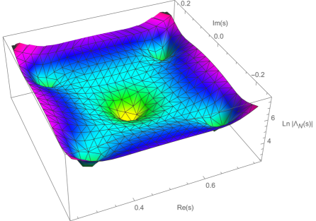
Figure 3. The closest 6 zeros of the approximation ฮ›Nโ€‹(E,s)subscriptฮ›๐‘๐ธ๐‘ \Lambda_{N}(E,s) to the central point, for all primes up to (and including) $p_{N=320}=2129$. This approximation is for the $L$-function associated to elliptic curve $y^{2}-x^{3}-5858x^{2}+111546435x=0$ of conductor $C=26799137200956120$ [11].
Refer to caption
Figure 4. Plot of lnโก|ฮ›Nโ€‹(E,s)|subscriptฮ›๐‘๐ธ๐‘ \ln|\Lambda_{N}(E,s)| in the central region for all primes up to (and including) $p_{N=250}=1583$, for the $L$-function associated to elliptic curve $y^{2}-x^{3}-1217x^{2}-96135x=0$, of conductor $C=421666952460$ [11]. The closest 5 zeros to the central point are clearly visible.

2. Preliminary facts

An elliptic curve $E$ over $\mathbb{Q}$ is a non-singular cubic curve given by an equation

(2.1) $$y^{2}=ax^{3}+bx^{2}+cx+d,$$

with $a,b,c,d\in\mathbb{Q}$, with aโ‰ 0๐‘Ž0a\neq 0. Let $p$ be a prime, and let $E_{p}$ be the curve over the finite field $\mathbb{F}_{p}$ obtained by reducing the coefficients of $E$ modulo $p$. We say that $E$ has good reduction at $p$ if $E_{p}$ is nonsingular, and has bad reduction at $p$ otherwise. The types of bad reduction at $p$ can be further classified into: additive (if $E_{p}$ has a cusp at its singular point), split multiplicative (if the singular point of $E_{p}$ is a node having two tangent lines with slopes in $\mathbb{F}_{p}$, rather than in an extension), and non-split multiplicative reduction. The conductor of $E$ is defined to be

(2.2) $$C=\prod_{p}p^{e_{p}},$$

where the exponent $e_{p}$ is zero if $E$ has good reduction at $p$, one if $E$ has multiplicative reduction at $p$, and two if $E$ has additive reduction and pโ‰ 2,3๐‘23p\neq 2,3 (if $p=2$ or $p=3$, the additive reduction case has a more complicated expression).

We define the $L$-series of an elliptic curve $E$ with conductor $C$ as the Euler product

(2.3) Lโ€‹(E,s)=โˆpโˆคC11โˆ’apโ€‹pโˆ’(s+1/2)+pโˆ’2โ€‹sโ€‹โˆpโˆฃC11+apโ€‹pโˆ’(s+1/2)๐ฟ๐ธ๐‘ subscriptproductnot-divides๐‘๐ถ11subscript๐‘Ž๐‘superscript๐‘๐‘ 12superscript๐‘2๐‘ subscriptproductconditional๐‘๐ถ11subscript๐‘Ž๐‘superscript๐‘๐‘ 12L(E,s)=\prod_{p\nmid C}\frac{1}{1-a_{p}p^{-(s+1/2)}+p^{-2s}}\prod_{p\mid C}\frac{1}{1+a_{p}p^{-(s+1/2)}}

which converges when โ„œโก(s)>1๐‘ 1\Re(s)>1. If $E$ has good reduction at $p$, $a_{p}=p+1-n_{p}$, where $n_{p}$ is the number of points of $E_{p}$. Otherwise, $a_{p}$ is zero in the case of bad additive reduction at $p$, $-1$ in the case of split multiplicative reduction and $+1$ otherwise.

The function Lโ€‹(E,s)๐ฟ๐ธ๐‘ L(E,s) admits an analytic continuation to the entire complex plane and a functional equation that relates the values at s๐‘ s with those at 1โˆ’s1๐‘ 1-s.

The critical line Reโ€‹(s)=1/2Re๐‘ 12\text{Re}(s)=1/2 of symmetry of the functional equation encodes important arithmetic information on the elliptic curve. The famous Birch and Swinnerton-Dyer conjecture posits that the analytic rank of $E$ which is defined to be the order of vanishing of $L(E,1/2)$, equals the rank of the finitely generated abelian group of rational points of $E$.

For the classical theory on the Riemann zeta function see [13] or [4]. For more on the theory of $L$-functions associated to elliptic curves the reader is referred to [8].

Our notations are as follows:

s๐‘ s the complex argument
$C$ the conductor
$w=(-1)^{P}$ the root number
Lpโ€‹(E,s)subscript๐ฟ๐‘๐ธ๐‘ L_{p}(E,s) the local factor at $p$
gโ€‹(s)๐‘”๐‘ g(s) the local factor at $\infty$
sโ‹†subscript๐‘ โ‹†s_{\star} complex variable running over the local factor poles
$\mathfrak{S}_{N}$ set of poles of all the local factors
$\mathfrak{O}_{N}$ set of poles of all the local factors at primes $p$
$r_{\star}$ residue at sโ‹†subscript๐‘ โ‹†s_{\star} of the local factor at $p$
$R_{-1/2-l}$ residue of gโ€‹(s)๐‘”๐‘ g(s) at negative half-integer $-1/2-l$
$p_{N}$ the cutoff in the number of primes

The local factor at the Archimedean place in analytic convention is

(2.4) gโ€‹(s)=Cs2โ€‹ฮ“โ„‚โ€‹(s+12),๐‘”๐‘ superscript๐ถ๐‘ 2subscriptฮ“โ„‚๐‘ 12g(s)=C^{\frac{s}{2}}\Gamma_{\mathbb{C}}\left(s+\frac{1}{2}\right),

where

(2.5) $$\Gamma_{\mathbb{C}}(z)\coloneqq 2(2\pi)^{-z}\Gamma(z),$$

with $\Gamma(z)$ the Euler Gamma function. In analytic convention the critical strip is 0<โ„œโก(s)<10๐‘ 10<\Re(s)<1 (see the $L$-function and modular forms database LMFDB.org for more details).

Remark 1.

In analytic convention, the inverse local factors at places of bad reduction are $1$, 1+pโˆ’sโˆ’1/21superscript๐‘๐‘ 121+p^{-s-1/2}, or 1โˆ’pโˆ’sโˆ’1/21superscript๐‘๐‘ 121-p^{-s-1/2}, depending on whether the bad reduction is additive, nonsplit multiplicative, or split multiplicative respectively.

We denote the local factor at $p$ in analytic convention by Lpโ€‹(E,s)subscript๐ฟ๐‘๐ธ๐‘ L_{p}(E,s), so that in the case of good reduction Lpโˆ’1โ€‹(E,s)=1โˆ’apโ€‹pโˆ’(s+1/2)+pโˆ’2โ€‹ssuperscriptsubscript๐ฟ๐‘1๐ธ๐‘ 1subscript๐‘Ž๐‘superscript๐‘๐‘ 12superscript๐‘2๐‘ L_{p}^{-1}(E,s)=1-a_{p}p^{-(s+1/2)}+p^{-2s}, and similar expressions hold at the places of bad reduction.

Remark 2 (Hasse bound).

The Hasse bound is

(2.6) $$|a_{p}|<2\sqrt{p}.$$

Coefficient $a_{p}$ is related to the number of points $n_{p}$ by the relation

(2.7) $$a_{p}=p+1-n_{p}.$$

The information in the $L$-function, according to our construction, will depend on the local $L$-factor poles. Lemmas 2.1 โ€“ 2.3 characterize the locations and types of these poles, in terms of reduction type.

Lemma 2.1.

In analytic convention, the poles of a local factor with good reduction are on the imaginary axis, and the poles of a local factor with bad multiplicative reduction are on the imaginary line of real partย ย โˆ’1/212-1/2.

For each prime $p$, Lpโ€‹(E,s)subscript๐ฟ๐‘๐ธ๐‘ L_{p}(E,s) has simple poles. The inverse of the local factor with good reductionย is

(2.8) Lpโˆ’1โ€‹(E,s)=1โˆ’apโ€‹pโˆ’(s+1/2)+pโˆ’2โ€‹s.subscriptsuperscript๐ฟ1๐‘๐ธ๐‘ 1subscript๐‘Ž๐‘superscript๐‘๐‘ 12superscript๐‘2๐‘ L^{-1}_{p}(E,s)=1-a_{p}p^{-(s+1/2)}+p^{-2s}.

If $a_{p}=0$ the result is immediate. Otherwise, the poles correspond to Lpโˆ’1โ€‹(E,s)=0superscriptsubscript๐ฟ๐‘1๐ธ๐‘ 0L_{p}^{-1}(E,s)=0, and are at

(2.9) sโ‹†=2โ€‹ฯ€โ€‹ilnโกpโ€‹k+1lnโกpโ€‹lnโก(apยฑiโ€‹4โ€‹pโˆ’ap22โ€‹p),kโˆˆโ„ค,formulae-sequencesubscript๐‘ โ‹†2๐œ‹๐‘–๐‘๐‘˜1๐‘plus-or-minussubscript๐‘Ž๐‘๐‘–4๐‘superscriptsubscript๐‘Ž๐‘22๐‘๐‘˜โ„คs_{\star}=\frac{2\pi i}{\ln p}k+\frac{1}{\ln p}\ln\left(\frac{a_{p}\pm i\sqrt{4p-a_{p}^{2}}}{2\sqrt{p}}\right),\quad k\in\mathbb{Z},

with residue

(2.10) $$r_{\star}=\frac{1}{2\ln p}\left(1\mp\frac{ia_{p}}{\sqrt{4p-a_{p}^{2}}}\right).$$

Note that precisely for $|a_{p}|<2\sqrt{p}$ (from the Hasse bound) the complex number inside the logarithm has unit norm, because

(2.11) $$\left(\frac{a_{p}}{2\sqrt{p}}\right)^{2}+\left(\frac{\sqrt{4p-a_{p}^{2}}}{2\sqrt{p}}\right)^{2}=1.$$

Thus the logarithm is purely imaginary, which proves the lemma in the case of good reduction. In the case of bad multiplicative reduction, the poles are the solutions of equation

(2.12) Lpโˆ’1โ€‹(E,s)=1ยฑpโˆ’sโˆ’12=0,subscriptsuperscript๐ฟ1๐‘๐ธ๐‘ plus-or-minus1superscript๐‘๐‘ 120L^{-1}_{p}(E,s)=1\pm p^{-s-\frac{1}{2}}=0,

so they will lie on the imaginary line of real part $-1/2$.

Remark 3.

Due to the strict inequality in the Hasse bound, the poles of local factors with good reduction cannot be at s=0๐‘ 0s=0, and similarly the poles of local factors with nonsplit bad multiplicative reduction cannot be on the real axis. However, the split multiplicative local factors all have a pole on the real axis, at s=โˆ’1/2๐‘ 12s=-1/2, which is also a pole for the local gamma factor at the Archimedean place.

Lemma 2.2.

All the poles of the local factors with bad multiplicative reduction are distinct, except for the possible poles at s=โˆ’1/2๐‘ 12s=-1/2.

Proof.

The locations of the poles are given by Eq. (2.12). Because the ratios of logarithms of prime numbers are irrational, the poles cannot coincide, except at $-1/2$. โˆŽ

Lemma 2.3.

Two distinct local factors with good reduction can have at most four common poles.

Proof.

Suppose the local factors with good reduction at $p$ and $q$, pโ‰ q๐‘๐‘žp\neq q, have a common pole at sโ‹†subscript๐‘ โ‹†s_{\star},ย then

(2.13) sโ‹†=2โ€‹ฯ€โ€‹ilnโกpโ€‹k+1lnโกpโ€‹lnโก(apยฑpiโ€‹4โ€‹pโˆ’ap22โ€‹p)=2โ€‹ฯ€โ€‹ilnโกqโ€‹l+1lnโกqโ€‹lnโก(aqยฑqiโ€‹4โ€‹qโˆ’aq22โ€‹q),subscript๐‘ โ‹†2๐œ‹๐‘–๐‘๐‘˜1๐‘subscriptplus-or-minus๐‘subscript๐‘Ž๐‘๐‘–4๐‘superscriptsubscript๐‘Ž๐‘22๐‘2๐œ‹๐‘–๐‘ž๐‘™1๐‘žsubscriptplus-or-minus๐‘žsubscript๐‘Ž๐‘ž๐‘–4๐‘žsuperscriptsubscript๐‘Ž๐‘ž22๐‘žs_{\star}=\frac{2\pi i}{\ln p}k+\frac{1}{\ln p}\ln\left(\frac{a_{p}\pm_{p}i\sqrt{4p-a_{p}^{2}}}{2\sqrt{p}}\right)=\frac{2\pi i}{\ln q}l+\frac{1}{\ln q}\ln\left(\frac{a_{q}\pm_{q}i\sqrt{4q-a_{q}^{2}}}{2\sqrt{q}}\right),

for $k,l\in\mathbb{Z}$ and one choice of signs $\pm_{p}$, $\pm_{q}$. There are four possible choices of signs total and for each choice there can be at most one pair of integers $k,l$ (because the ratio $\ln q/\ln p$ is irrational), thus the local factors can share at most four poles. โˆŽ

For $\sigma,t\in\mathbb{R}$, $-\sigma\notin\mathbb{N}$, the gamma function obeys the identity

(2.14) $$|\Gamma\left(\sigma+it\right)|=|\Gamma(\sigma)|\prod_{k=0}^{\infty}\left(1+\frac{t^{2}}{(\sigma+k)^{2}}\right)^{-\frac{1}{2}},$$

which can be used to prove the following standard result that we will need later.

Lemma 2.4.

For real $\sigma\geqslant 1$ and real $t$ we have

(2.15) $$\left|\frac{\Gamma\left(\sigma+it\right)}{\Gamma\left(\sigma\right)}\right|\ll e^{-\frac{3}{8}\min\left(|t|,\frac{t^{2}}{\sigma}\right)}.$$

3. A family of approximations for Hasse-Weil $L$-functions

As we will show, the generalization of Matiyasevichโ€™s prescription [9] for the case of $L$-functions associated to elliptic curves constructs a function $\Lambda_{N}$ that approximates the $L$-function $\Lambda$ in the limit $N\to\infty$. Here $N$ is the number of primes included in the approximation, and when $N$ is large ฮ›Nโ€‹(E,s)subscriptฮ›๐‘๐ธ๐‘ \Lambda_{N}(E,s) approximates ฮ›โ€‹(E,s)ฮ›๐ธ๐‘ \Lambda(E,s) with exponential precision in $p_{N+1}$,

(3.1) ฮ›โ€‹(E,s0)โˆ’ฮ›Nโ€‹(E,s0)ฮ›๐ธsubscript๐‘ 0subscriptฮ›๐‘๐ธsubscript๐‘ 0\displaystyle\Lambda(E,s_{0})-\Lambda_{N}(E,s_{0}) $\displaystyle=$ apN+1โ€‹C14ฯ€โ€‹pN+1โ€‹eโˆ’2โ€‹ฯ€โ€‹pN+1Cโ€‹[1+(โˆ’1)P+(2โ€‹s0โˆ’1)โ€‹C124โ€‹ฯ€โ€‹pN+1โ€‹(1โˆ’(โˆ’1)P)+๐’ชโ€‹(pN+1โˆ’2)]subscript๐‘Žsubscript๐‘๐‘1superscript๐ถ14๐œ‹subscript๐‘๐‘1superscript๐‘’2๐œ‹subscript๐‘๐‘1๐ถdelimited-[]1superscript1๐‘ƒ2subscript๐‘ 01superscript๐ถ124๐œ‹subscript๐‘๐‘11superscript1๐‘ƒ๐’ชsuperscriptsubscript๐‘๐‘12\displaystyle\frac{a_{p_{N+1}}C^{\frac{1}{4}}}{\pi p_{N+1}}e^{-\frac{2\pi p_{N+1}}{\sqrt{C}}}\left[1+(-1)^{P}+\frac{(2s_{0}-1)C^{\frac{1}{2}}}{4\pi p_{N+1}}\left(1-(-1)^{P}\right)+\mathcal{O}(p_{N+1}^{-2})\right]
$\displaystyle+\mathcal{O}\left(\frac{1}{\left(p_{N+2}\right)^{1-(-1)^{P}/2}}e^{-\frac{2\pi p_{N+2}}{\sqrt{C}}}\right)$

(see Theorem 5 for the details). $\Lambda_{N}$ is a sum of two terms,

(3.2) ฮ›Nโ€‹(E,s)โ‰”ฮ›Ningoingโ€‹(E,s)+(โˆ’1)Pโ€‹ฮ›Ningoingโ€‹(E,1โˆ’s),โ‰”subscriptฮ›๐‘๐ธ๐‘ subscriptsuperscriptฮ›ingoing๐‘๐ธ๐‘ superscript1๐‘ƒsubscriptsuperscriptฮ›ingoing๐‘๐ธ1๐‘ \Lambda_{N}(E,s)\coloneqq\Lambda^{\mathrm{ingoing}}_{N}(E,s)+(-1)^{P}\Lambda^{\mathrm{ingoing}}_{N}(E,1-s),

where the root number $(-1)^{P}$ is the sign in the ฮ›โ€‹(E,s)ฮ›๐ธ๐‘ \Lambda(E,s) functional equation, which reads

(3.3) ฮ›โ€‹(E,s)=(โˆ’1)Pโ€‹ฮ›โ€‹(E,1โˆ’s).ฮ›๐ธ๐‘ superscript1๐‘ƒฮ›๐ธ1๐‘ \Lambda(E,s)=(-1)^{P}\Lambda(E,1-s).

In order to construct the function ฮ›Ningoingโ€‹(E,s)subscriptsuperscriptฮ›ingoing๐‘๐ธ๐‘ \Lambda^{\mathrm{ingoing}}_{N}(E,s) we must first construct a finite Euler product ฮ›NEulerโ€‹(E,s)superscriptsubscriptฮ›๐‘Euler๐ธ๐‘ \Lambda_{N}^{\mathrm{Euler}}(E,s), that is

(3.4) ฮ›NEulerโ€‹(E,s)โ‰”gโ€‹(s)โ€‹โˆp=2pNLpโ€‹(E,s),โ‰”superscriptsubscriptฮ›๐‘Euler๐ธ๐‘ ๐‘”๐‘ superscriptsubscriptproduct๐‘2subscript๐‘๐‘subscript๐ฟ๐‘๐ธ๐‘ \Lambda_{N}^{\mathrm{Euler}}(E,s)\coloneqq g(s)\prod_{p=2}^{p_{N}}L_{p}(E,s),

where the product is understood to run over primes. The right-hand side of Eq. (3.4) is a meromorphic function with an infinite number of poles in the complex plane, at s=sโ‹†๐‘ subscript๐‘ โ‹†s=s_{\star} with Lpโˆ’1โ€‹(sโ‹†)=0subscriptsuperscript๐ฟ1๐‘subscript๐‘ โ‹†0L^{-1}_{p}(s_{\star})=0 for all primes $2\leqslant p\leqslant p_{N}$, and at s=โˆ’lโˆ’1/2๐‘ ๐‘™12s=-l-1/2, $l\in\mathbb{N}$, corresponding to the poles of gโ€‹(s)๐‘”๐‘ g(s). Note that if the curve has split multiplicative reduction then s=โˆ’1/2๐‘ 12s=-1/2 is a pole both for gโ€‹(s)๐‘”๐‘ g(s) and the split multiplicative local factors, and so ฮ›NEulerโ€‹(E,s)superscriptsubscriptฮ›๐‘Euler๐ธ๐‘ \Lambda_{N}^{\mathrm{Euler}}(E,s) will have a higher order pole at s=โˆ’1/2๐‘ 12s=-1/2.

As explained in Lemmas 2.1, 2.2, any pole of a bad reduction local factor cannot coincide with any other poles, except possibly at s=โˆ’1/2๐‘ 12s=-1/2. In the rest of the paper we will remain agnostic whether poles of different good reduction local factors can coincide. For each good reduction local factor pole sโ‹†subscript๐‘ โ‹†s_{\star} we will assume an order $k_{\star}\geqslant 1$ of the pole in ฮ›NEulerโ€‹(E,s)superscriptsubscriptฮ›๐‘Euler๐ธ๐‘ \Lambda_{N}^{\mathrm{Euler}}(E,s). Note that, because we are considering a finite number of primes $p\leqslant p_{N}$, $k_{\star}$ must be finite, from Lemma 2.3.

The next step is to construct the principal part ฮ›Nppโ€‹(E,s)subscriptsuperscriptฮ›pp๐‘๐ธ๐‘ \Lambda^{\mathrm{pp}}_{N}(E,s) of ฮ›NEulerโ€‹(E,s)superscriptsubscriptฮ›๐‘Euler๐ธ๐‘ \Lambda_{N}^{\mathrm{Euler}}(E,s). Consider the infinite set $\mathfrak{S}_{N}$ of all the local factor poles,

(3.5) ๐”–Nโ‰”{sโ‹†|LpโฉฝpNโˆ’1โ€‹(E,sโ‹†)=0}โˆช{sโ‹†|gโˆ’1โ€‹(sโ‹†)=0}.โ‰”subscript๐”–๐‘conditional-setsubscript๐‘ โ‹†superscriptsubscript๐ฟ๐‘subscript๐‘๐‘1๐ธsubscript๐‘ โ‹†0conditional-setsubscript๐‘ โ‹†superscript๐‘”1subscript๐‘ โ‹†0\mathfrak{S}_{N}\coloneqq\left\{s_{\star}|L_{p\leqslant p_{N}}^{-1}(E,s_{\star})=0\right\}\cup\left\{s_{\star}|g^{-1}(s_{\star})=0\right\}.

The Laurent series of ฮ›NEulerโ€‹(E,s)superscriptsubscriptฮ›๐‘Euler๐ธ๐‘ \Lambda_{N}^{\mathrm{Euler}}(E,s) around each sโ‹†โˆˆ๐”–Nsubscript๐‘ โ‹†subscript๐”–๐‘s_{\star}\in\mathfrak{S}_{N},

(3.6) ฮ›NEulerโ€‹(E,s)=โˆ‘k=โˆ’kโ‹†โˆžฯโ‹†(k)โ€‹(sโˆ’sโ‹†)k,superscriptsubscriptฮ›๐‘Euler๐ธ๐‘ superscriptsubscript๐‘˜subscript๐‘˜โ‹†subscriptsuperscript๐œŒ๐‘˜โ‹†superscript๐‘ subscript๐‘ โ‹†๐‘˜\Lambda_{N}^{\mathrm{Euler}}(E,s)=\sum_{k=-k_{\star}}^{\infty}\rho^{(k)}_{\star}\left(s-s_{\star}\right)^{k},

has a principal part

(3.7) ฮ›Npp,sโ‹†โ€‹(E,s)โ‰”โˆ‘k=โˆ’kโ‹†โˆ’1ฯโ‹†(k)โ€‹(sโˆ’sโ‹†)k.โ‰”superscriptsubscriptฮ›๐‘ppsubscript๐‘ โ‹†๐ธ๐‘ superscriptsubscript๐‘˜subscript๐‘˜โ‹†1subscriptsuperscript๐œŒ๐‘˜โ‹†superscript๐‘ subscript๐‘ โ‹†๐‘˜\Lambda_{N}^{\mathrm{pp},s_{\star}}(E,s)\coloneqq\sum_{k=-k_{\star}}^{-1}\rho^{(k)}_{\star}\left(s-s_{\star}\right)^{k}.

The principal part ฮ›Nppโ€‹(E,s)subscriptsuperscriptฮ›pp๐‘๐ธ๐‘ \Lambda^{\mathrm{pp}}_{N}(E,s) of ฮ›NEulerโ€‹(E,s)superscriptsubscriptฮ›๐‘Euler๐ธ๐‘ \Lambda_{N}^{\mathrm{Euler}}(E,s) is defined as the sum

(3.8) ฮ›Nppโ€‹(E,s)โ‰”โˆ‘sโ‹†โˆˆ๐”–Nฮ›Npp,sโ‹†โ€‹(E,s),โ‰”subscriptsuperscriptฮ›pp๐‘๐ธ๐‘ subscriptsubscript๐‘ โ‹†subscript๐”–๐‘superscriptsubscriptฮ›๐‘ppsubscript๐‘ โ‹†๐ธ๐‘ \Lambda^{\mathrm{pp}}_{N}(E,s)\coloneqq\sum_{s_{\star}\in\mathfrak{S}_{N}}\Lambda_{N}^{\mathrm{pp},s_{\star}}(E,s),

and ฮ›Ningoingโ€‹(E,s)subscriptsuperscriptฮ›ingoing๐‘๐ธ๐‘ \Lambda^{\mathrm{ingoing}}_{N}(E,s) is defined as

(3.9) ฮ›Ningoingโ€‹(E,s)โ‰”ฮ›NEulerโ€‹(E,s)โˆ’ฮ›Nppโ€‹(E,s).โ‰”subscriptsuperscriptฮ›ingoing๐‘๐ธ๐‘ subscriptsuperscriptฮ›Euler๐‘๐ธ๐‘ subscriptsuperscriptฮ›pp๐‘๐ธ๐‘ \Lambda^{\mathrm{ingoing}}_{N}(E,s)\coloneqq\Lambda^{\mathrm{Euler}}_{N}(E,s)-\Lambda^{\mathrm{pp}}_{N}(E,s).

The principal part ฮ›Nppโ€‹(E,s)superscriptsubscriptฮ›๐‘pp๐ธ๐‘ \Lambda_{N}^{\mathrm{pp}}(E,s) in Eq. (3.8) is well-defined, meaning that the sum over sโ‹†โˆˆ๐”–Nsubscript๐‘ โ‹†subscript๐”–๐‘s_{\star}\in\mathfrak{S}_{N} converges, as we explain in Remarks 4, 5.

Remark 4.

Let

(3.10) $$\mathfrak{O}_{N}\coloneqq\mathfrak{S}_{N}-\{-l-1/2\,|\,l\in\mathbb{N}\}$$

be the set of local factor poles not at the negative half-integers. The sum in Eq. (3.8) over sโ‹†โˆˆ๐”’NโŠ‚๐”–Nsubscript๐‘ โ‹†subscript๐”’๐‘subscript๐”–๐‘s_{\star}\in\mathfrak{O}_{N}\subset\mathfrak{S}_{N} converges, because the factor of gโ€‹(sโ‹†)๐‘”subscript๐‘ โ‹†g(s_{\star}) decays rapidly at large absolute value of โ„‘โก(sโ‹†)subscript๐‘ โ‹†\Im\left(s_{\star}\right).

Remark 5.

Let $R_{-l-1/2}$ be the residue of gโ€‹(s)๐‘”๐‘ g(s) at the negative half-integer $-l-1/2$, $l\in\mathbb{N}$. We have that $R_{-1/2}=2/C^{1/4}$, and from the identity $\Gamma(z+1)=z\Gamma(z)$ it follows that

(3.11) $$R_{-(l+1)-1/2}=R_{-l-1/2}\frac{-2\pi}{\sqrt{C}(l+1)},$$

so that the residues at the negative half-integers decay rapidly in the real negative direction. Thus the sum in Eq. (3.8) over sโ‹†โˆˆ{โˆ’lโˆ’1/2|lโˆˆโ„•}โŠ‚๐”–Nsubscript๐‘ โ‹†conditional-set๐‘™12๐‘™โ„•subscript๐”–๐‘s_{\star}\in\{-l-1/2\,|\,l\in\mathbb{N}\}\subset\mathfrak{S}_{N} converges.

Remark 6.

ฮ›Ningoingโ€‹(E,s)subscriptsuperscriptฮ›ingoing๐‘๐ธ๐‘ \Lambda^{\mathrm{ingoing}}_{N}(E,s) in Eq. (3.9) and ฮ›Nโ€‹(E,s)subscriptฮ›๐‘๐ธ๐‘ \Lambda_{N}(E,s) in Eq. (3.2) are entire.

Example 1.

To illustrate this prescription on an example, consider an $L$-function arising from an elliptic curve with only bad additive reduction. Furthermore, suppose that all orders of the good place local factor poles are $k_{\star}=1$. Then the prescription reads

ฮ›Ningoingโ€‹(E,s)subscriptsuperscriptฮ›ingoing๐‘๐ธ๐‘ \displaystyle\Lambda^{\mathrm{ingoing}}_{N}(E,s) $\displaystyle=$ gโ€‹(s)โ€‹โˆp=2pNLpโ€‹(E,s)โˆ’โˆ‘sโ‹†โˆˆ๐”’Ngโ€‹(sโ‹†)โ€‹โˆp=2pโˆคCLpโˆ’1โ€‹(sโ‹†)โ‰ 0pNLpโ€‹(E,sโ‹†)โ€‹rโ‹†sโˆ’sโ‹†๐‘”๐‘ superscriptsubscriptproduct๐‘2subscript๐‘๐‘subscript๐ฟ๐‘๐ธ๐‘ subscriptsubscript๐‘ โ‹†subscript๐”’๐‘๐‘”subscript๐‘ โ‹†superscriptsubscriptproduct๐‘2not-divides๐‘๐ถsubscriptsuperscript๐ฟ1๐‘subscript๐‘ โ‹†0subscript๐‘๐‘subscript๐ฟ๐‘๐ธsubscript๐‘ โ‹†subscript๐‘Ÿโ‹†๐‘ subscript๐‘ โ‹†\displaystyle g(s)\prod_{p=2}^{p_{N}}L_{p}(E,s)-\sum_{s_{\star}\in\mathfrak{O}_{N}}g(s_{\star})\prod_{\begin{subarray}{c}p=2\\ p\,\nmid\,C\\ L^{-1}_{p}(s_{\star})\neq 0\end{subarray}}^{p_{N}}L_{p}(E,s_{\star})\frac{r_{\star}}{s-s_{\star}}
$\displaystyle-$ โˆ‘l=0โˆžโˆp=2pโˆคCpNLpโ€‹(E,โˆ’lโˆ’1/2)โ€‹Rโˆ’lโˆ’1/2s+l+1/2,superscriptsubscript๐‘™0superscriptsubscriptproduct๐‘2not-divides๐‘๐ถsubscript๐‘๐‘subscript๐ฟ๐‘๐ธ๐‘™12subscript๐‘…๐‘™12๐‘ ๐‘™12\displaystyle\sum_{l=0}^{\infty}\prod_{\begin{subarray}{c}p=2\\ p\,\nmid\,C\end{subarray}}^{p_{N}}L_{p}(E,-l-1/2)\frac{R_{-l-1/2}}{s+l+1/2},

with sโ‹†subscript๐‘ โ‹†s_{\star} and $r_{\star}$ given by Eqs. (2.9) and (2.10) respectively.

4. The effectiveness and error of the approximations

We now prove that our family approximates the degree $2$ $L$-function ฮ›โ€‹(E,s)ฮ›๐ธ๐‘ \Lambda(E,s). Our argument will involve integrating along certain contours in the complex plane that, for an approximation ฮ›Nโ€‹(E,s)subscriptฮ›๐‘๐ธ๐‘ \Lambda_{N}(E,s), are chosen to avoid in a controlled manner all the local factor poles in ฮ›NEulerโ€‹(E,s)superscriptsubscriptฮ›๐‘Euler๐ธ๐‘ \Lambda_{N}^{\mathrm{Euler}}(E,s). These contours are introduced in Definition 3. Lemmas 4.1, 4.2 characterize these contours and obtain upper bounds for ฮ›Nppโ€‹(E,s)superscriptsubscriptฮ›๐‘pp๐ธ๐‘ \Lambda_{N}^{\mathrm{pp}}(E,s) for s๐‘ s on the contours.

Definition 3.

A closed contour $\mathcal{C}$ in the complex plane is sparse w.r.t. $\mathfrak{S}_{N}$ if for sโˆˆ๐’ž๐‘ ๐’žs\in\mathcal{C} we have

(4.1) minpโฉฝpNโกminsโ‹†โˆˆ๐”’Nโก|sโˆ’sโ‹†|โ‰ซ1pNmuch-greater-thansubscript๐‘subscript๐‘๐‘subscriptsubscript๐‘ โ‹†subscript๐”’๐‘๐‘ subscript๐‘ โ‹†1subscript๐‘๐‘\min_{p\leqslant p_{N}}\min_{s_{\star}\in\mathfrak{O}_{N}}\left|s-s_{\star}\right|\gg\frac{1}{p_{N}}

and

(4.2) minlโˆˆโ„•โก|s+l+12|โ‰ซ1.much-greater-thansubscript๐‘™โ„•๐‘ ๐‘™121\min_{l\in\mathbb{N}}|s+l+\frac{1}{2}|\gg 1.
Lemma 4.1.

There exist arbitrarily large rectangular contours $\mathcal{C}$ (in the sense that the coordinates of the $4$ vertices can be arbitrarily large in the real and imaginary directions) that are sparse w.r.t.ย ๐”–Nsubscript๐”–๐‘\mathfrak{S}_{N}.

Proof.

To satisfy Eq. (4.2), it suffices to pick the vertical part of the contour to pass through the middle point between two poles of the local gamma factor. For Eq.ย (4.1), note that on any vertical interval of length $1$ on the imaginary axis, from the prime number theorem there are $\mathcal{O}\left(p_{N}/\ln p_{N}\right)$ prime numbers $\leqslant p_{N}$. For prime $p$ the poles are spaced $\mathcal{O}\left(1/\ln p\right)$ apart, so there will be $\mathcal{O}\left(\ln p\right)$ poles in an interval of length $1$, so in such an interval there will be at most $\mathcal{O}\left(p_{N}\right)$ poles total. Then, by the pigeonhole principle, it is possible to draw the horizontal part of the contour so that Eq. (4.1) holds. โˆŽ

Lemma 4.2.

With the notations above, uniformly for all sโˆˆโ„‚๐‘ โ„‚s\in\mathbb{C} on a sparse contour wrt. $\mathfrak{S}_{N}$, we have

(4.3) |ฮ›Nppโ€‹(E,s)|โ‰ช11+|s|,much-less-thansubscriptsuperscriptฮ›pp๐‘๐ธ๐‘ 11๐‘ \left|\Lambda^{\mathrm{pp}}_{N}(E,s)\right|\ll\frac{1}{1+|s|},

where the constant implied by the $\ll$ symbol depends on the $L$-function and $N$ only.

Proof.

From Eqs. (2.4), (2.5) we have

(4.4) gโ€‹(s)=232โˆ’sโ€‹ฯ€โˆ’sโˆ’12โ€‹Cs/21+2โ€‹sโ€‹ฮ“โ€‹(s+32),๐‘”๐‘ superscript232๐‘ superscript๐œ‹๐‘ 12superscript๐ถ๐‘ 212๐‘ ฮ“๐‘ 32g(s)=\frac{2^{\frac{3}{2}-s}\pi^{-s-\frac{1}{2}}C^{s/2}}{1+2s}\Gamma\left(s+\frac{3}{2}\right),

so that from Eq. (2.15), for s๐‘ s of large imaginary part on the imaginary axis, we have

(4.5) |gโ€‹(s)|โฉฝC1โ€‹eโˆ’C2โ€‹โ„‘โก(s),๐‘”๐‘ subscript๐ถ1superscript๐‘’subscript๐ถ2๐‘ |g(s)|\leqslant C_{1}e^{-C_{2}\Im\left(s\right)},

for some constants $C_{1,2}>0$. Consider now the poles at sโ‹†subscript๐‘ โ‹†s_{\star} with Lโฉฝโ„‘โก(sโ‹†)<L+1๐ฟsubscript๐‘ โ‹†๐ฟ1L\leqslant\Im(s_{\star})<L+1 for nonnegative integer $L$, Eq. (4.5) implies that

(4.6) maxLโฉฝsโ‹†<L+1โกmax1โฉฝkโฉฝkโ‹†โก|ฯโ‹†(โˆ’k)|โฉฝCNโ€‹eโˆ’C0โ€‹L,subscript๐ฟsubscript๐‘ โ‹†๐ฟ1subscript1๐‘˜subscript๐‘˜โ‹†subscriptsuperscript๐œŒ๐‘˜โ‹†subscript๐ถ๐‘superscript๐‘’subscript๐ถ0๐ฟ\max_{L\leqslant s_{\star}<L+1}\max_{1\leqslant k\leqslant k_{\star}}\left|\rho^{(-k)}_{\star}\right|\leqslant C_{N}e^{-C_{0}L},

where $k_{\star}$ is the order of the pole at sโ‹†subscript๐‘ โ‹†s_{\star} and $\rho_{\star}^{(-k)}$ are the coefficients in the Laurent expansion (3.6). This inequality holds due to the factor of gโ€‹(sโ‹†)๐‘”subscript๐‘ โ‹†g(s_{\star}) in each $\rho^{(-k)}_{\star}$. Here the constant $C_{0}$ depends only on the given $L$-function, and the constant $C_{N}$ depends only on $N$ and the $L$-function. We remark that there exists an $L_{0}$ depending only on $N$ and the $L$-function, such that for all $L\geqslant L_{0}$ all the poles in Eq. (4.6) will be simple, by Lemma 2.3 and the fact that the poles in the local factors not at s=โˆ’1/2๐‘ 12s=-1/2 are simple. It follows that, for all $L\geqslant L_{0}$, Eq. (4.6) reduces to

(4.7) maxpjโฉฝpNpjโ€‹ย notโ€‰ badโ€‰ additiveโกmaxLโฉฝsโ‹†<L+1Lpjโ€‹(sโ‹†)=0โก|gโ€‹(sโ‹†)โ€‹rโ‹†โ€ฒโ€‹(โˆp=2pโ‰ pjp|CpN11โˆ’apbadโ€‹pโˆ’sโ‹†โˆ’1/2)โ€‹(โˆp=2pโ‰ pjpโˆคCpN11โˆ’apโ€‹pโˆ’(sโ‹†+1/2)+pโˆ’2โ€‹sโ‹†)|โฉฝCpNโ€‹eโˆ’C0โ€‹L,subscriptsubscript๐‘๐‘—subscript๐‘๐‘subscript๐‘๐‘—ย notโ€‰ badโ€‰ additivesubscript๐ฟsubscript๐‘ โ‹†๐ฟ1subscript๐ฟsubscript๐‘๐‘—subscript๐‘ โ‹†0๐‘”subscript๐‘ โ‹†subscriptsuperscript๐‘Ÿโ€ฒโ‹†superscriptsubscriptproduct๐‘2๐‘subscript๐‘๐‘—conditional๐‘๐ถsubscript๐‘๐‘11subscriptsuperscript๐‘Žbad๐‘superscript๐‘subscript๐‘ โ‹†12superscriptsubscriptproduct๐‘2๐‘subscript๐‘๐‘—not-divides๐‘๐ถsubscript๐‘๐‘11subscript๐‘Ž๐‘superscript๐‘subscript๐‘ โ‹†12superscript๐‘2subscript๐‘ โ‹†subscript๐ถsubscript๐‘๐‘superscript๐‘’subscript๐ถ0๐ฟ\max_{\begin{subarray}{c}p_{j}\leqslant p_{N}\\ p_{j}\text{\, not\, bad\, additive}\end{subarray}}\max_{\begin{subarray}{c}L\leqslant s_{\star}<L+1\\ L_{p_{j}}(s_{\star})=0\end{subarray}}\Bigg{|}g(s_{\star})r^{\prime}_{\star}\Bigg{(}\prod_{\begin{subarray}{c}p=2\\ p\neq p_{j}\\ p\,|\,C\end{subarray}}^{p_{N}}\frac{1}{1-a^{\mathrm{bad}}_{p}p^{-s_{\star}-1/2}}\Bigg{)}\Bigg{(}\prod_{\begin{subarray}{c}p=2\\ p\neq p_{j}\\ p\,\nmid\,C\end{subarray}}^{p_{N}}\frac{1}{1-a_{p}p^{-(s_{\star}+1/2)}+p^{-2s_{\star}}}\Bigg{)}\Bigg{|}\leqslant C_{p_{N}}e^{-C_{0}L},

where $a_{p}^{\mathrm{bad}}\in\{-1,0,1\}$, depending on the type of reduction, and

(4.8) $$r^{\prime}_{\star}=\begin{cases}r_{\star}\text{\quad if\ }p_{j}\nmid C,\\ \frac{1}{\ln p_{j}}\text{\ if\ }p_{j}\text{\ is\ bad\ multiplicative}\end{cases}.$$

We now consider an |s|>2โ€‹L0๐‘ 2subscript๐ฟ0|s|>2L_{0}, and split into four cases,

(4.9) Lโ€‹{โฉฝL0โˆˆ(L0,โŒˆ|s|2โŒ‰]โˆˆ(โŒˆ|s|2โŒ‰,โŒˆ2โ€‹|s|โŒ‰)โฉพโŒˆ2โ€‹|s|โŒ‰.๐ฟcasesabsentsubscript๐ฟ0otherwiseabsentsubscript๐ฟ0๐‘ 2otherwiseabsent๐‘ 22๐‘ otherwiseabsent2๐‘ otherwise\displaystyle L\begin{cases}\leqslant L_{0}\\ \in\left(L_{0}\ ,\left\lceil\frac{|s|}{2}\right\rceil\right]\\ \in\left(\left\lceil\frac{|s|}{2}\right\rceil,\left\lceil 2|s|\right\rceil\right)\\ \geqslant\left\lceil 2|s|\right\rceil\end{cases}.

For $L\leqslant L_{0}$, we have that

(4.10) โˆ‘L=1L0โˆ‘Lโฉฝsโ‹†<L+1โˆ‘1โฉฝkโฉฝkโ‹†|ฯโ‹†(โˆ’k)||sโˆ’sโ‹†|kโฉฝCN(0)1+|s|.superscriptsubscript๐ฟ1subscript๐ฟ0subscript๐ฟsubscript๐‘ โ‹†๐ฟ1subscript1๐‘˜subscript๐‘˜โ‹†subscriptsuperscript๐œŒ๐‘˜โ‹†superscript๐‘ subscript๐‘ โ‹†๐‘˜subscriptsuperscript๐ถ0๐‘1๐‘ \sum_{L=1}^{L_{0}}\sum_{L\leqslant s_{\star}<L+1}\sum_{1\leqslant k\leqslant k_{\star}}\frac{\left|\rho^{(-k)}_{\star}\right|}{|s-s_{\star}|^{k}}\leqslant\frac{C^{(0)}_{N}}{1+|s|}.

For Lโˆˆ(L0,โŒˆ|s|2โŒ‰]๐ฟsubscript๐ฟ0๐‘ 2L\in\left(L_{0}\ ,\left\lceil\frac{|s|}{2}\right\rceil\right], we have that

(4.11) โˆ‘L=L0+1โŒˆ|s|2โŒ‰โˆ‘pjโฉฝpNpjโ€‹ย notโ€‰ badโ€‰ additiveโˆ‘Lโฉฝsโ‹†<L+1Lpjโ€‹(sโ‹†)=0|g(sโ‹†)rโ‹†โ€ฒ(โˆp=2pโ‰ pjp|CpN11โˆ’apbadโ€‹pโˆ’sโ‹†โˆ’1/2)ร—\displaystyle\sum_{L=L_{0}+1}^{\left\lceil\frac{|s|}{2}\right\rceil}\sum_{\begin{subarray}{c}p_{j}\leqslant p_{N}\\ p_{j}\text{\, not\, bad\, additive}\end{subarray}}\sum_{\begin{subarray}{c}L\leqslant s_{\star}<L+1\\ L_{p_{j}}(s_{\star})=0\end{subarray}}\Bigg{|}g(s_{\star})r^{\prime}_{\star}\Bigg{(}\prod_{\begin{subarray}{c}p=2\\ p\neq p_{j}\\ p\,|\,C\end{subarray}}^{p_{N}}\frac{1}{1-a^{\mathrm{bad}}_{p}p^{-s_{\star}-1/2}}\Bigg{)}\times
ร—(โˆp=2pโ‰ pjpโˆคCpN11โˆ’apโ€‹pโˆ’(sโ‹†+1/2)+pโˆ’2โ€‹sโ‹†)|1|sโˆ’sโ‹†|โฉฝCN(1)1+|s|.\displaystyle\times\Bigg{(}\prod_{\begin{subarray}{c}p=2\\ p\neq p_{j}\\ p\,\nmid\,C\end{subarray}}^{p_{N}}\frac{1}{1-a_{p}p^{-(s_{\star}+1/2)}+p^{-2s_{\star}}}\Bigg{)}\Bigg{|}\frac{1}{|s-s_{\star}|}\leqslant\frac{C^{(1)}_{N}}{1+|s|}.

For LโฉพโŒˆ2โ€‹|s|โŒ‰๐ฟ2๐‘ L\geqslant\left\lceil 2|s|\right\rceil, we have that

(4.12) โˆ‘L=โŒˆ2โ€‹|s|โŒ‰โˆžeโˆ’C0โ€‹L=e(1โˆ’โŒˆ2โ€‹|s|โŒ‰)โ€‹C0eC0โˆ’1โฉฝCN(2)1+|s|.superscriptsubscript๐ฟ2๐‘ superscript๐‘’subscript๐ถ0๐ฟsuperscript๐‘’12๐‘ subscript๐ถ0superscript๐‘’subscript๐ถ01subscriptsuperscript๐ถ2๐‘1๐‘ \sum_{L=\left\lceil 2|s|\right\rceil}^{\infty}e^{-C_{0}L}=\frac{e^{\left(1-\left\lceil 2|s|\right\rceil\right)C_{0}}}{e^{C_{0}}-1}\leqslant\frac{C^{(2)}_{N}}{1+|s|}.

In Eqs. (4.10) โ€“ (4.12), $C^{(0)}_{N}$ $C^{(1)}_{N}$, $C^{(2)}_{N}$ are constants that depend on $N$ and on the $L$-function.

For โŒˆ|s|/2โŒ‰<L<โŒˆ2โ€‹|s|โŒ‰๐‘ 2๐ฟ2๐‘ \left\lceil|s|/2\right\rceil<L<\left\lceil 2|s|\right\rceil, we have that โˆ‘L=โŒˆ|s|2โŒ‰โŒˆ2โ€‹|s|โŒ‰eโˆ’C0โ€‹Lsuperscriptsubscript๐ฟ๐‘ 22๐‘ superscript๐‘’subscript๐ถ0๐ฟ\sum_{L=\left\lceil\frac{|s|}{2}\right\rceil}^{\left\lceil 2|s|\right\rceil}e^{-C_{0}L} decays exponentially when |s|๐‘ |s| is large, and the sparseness condition ensures that there can be no large contribution in s๐‘ s coming from the factors of |sโˆ’sโ‹†|๐‘ subscript๐‘ โ‹†|s-s_{\star}| in the denominator. We have thus obtained

(4.13) |ฮ›Nppโ€‹(E,s)|โฉฝCNโ€ฒ1+|s|subscriptsuperscriptฮ›pp๐‘๐ธ๐‘ subscriptsuperscript๐ถโ€ฒ๐‘1๐‘ \left|\Lambda^{\mathrm{pp}}_{N}(E,s)\right|\leqslant\frac{C^{\prime}_{N}}{1+|s|}

uniformly for s๐‘ s on the sparse contours w.r.t. $\mathfrak{S}_{N}$, where $C^{\prime}_{N}$ is a constant that depends on $N$, the $L$-function being considered, as well as on the implicit constants in Eqs. (4.1), (4.2). โˆŽ

We now need to estimate the difference between the $L$-function ฮ›โ€‹(E,s)ฮ›๐ธ๐‘ \Lambda(E,s) and the approximation ฮ›Nโ€‹(E,s)subscriptฮ›๐‘๐ธ๐‘ \Lambda_{N}(E,s). Theorem (4) expresses this difference as an integral of ฮ›โ€‹(E,s)โˆ’ฮ›NEulerโ€‹(E,s)ฮ›๐ธ๐‘ subscriptsuperscriptฮ›Euler๐‘๐ธ๐‘ \Lambda(E,s)-\Lambda^{\mathrm{Euler}}_{N}(E,s) on a vertical line to the right of the critical strip. This integral presentation will allow us to obtain asymptotic formulas for the difference ฮ›โ€‹(E,s0)โˆ’ฮ›Nโ€‹(E,s0)ฮ›๐ธsubscript๐‘ 0subscriptฮ›๐‘๐ธsubscript๐‘ 0\Lambda(E,s_{0})-\Lambda_{N}(E,s_{0}) at any given point s0subscript๐‘ 0s_{0}.

Theorem 4.

For any s0โˆˆโ„‚subscript๐‘ 0โ„‚s_{0}\in\mathbb{C}, elliptic curve $L$-function ฮ›โ€‹(E,s)ฮ›๐ธ๐‘ \Lambda(E,s), and $\sigma>1$, we have

(4.14) ฮ›โ€‹(E,s0)โˆ’ฮ›Nโ€‹(E,s0)=12โ€‹ฯ€โ€‹iโ€‹โˆซโ„œโก(s)=ฯƒ[ฮ›โ€‹(E,s)โˆ’ฮ›NEulerโ€‹(E,s)]โ€‹(1sโˆ’s0+(โˆ’1)Pโ€‹1sโˆ’1+s0),ฮ›๐ธsubscript๐‘ 0subscriptฮ›๐‘๐ธsubscript๐‘ 012๐œ‹๐‘–subscript๐‘ ๐œŽdelimited-[]ฮ›๐ธ๐‘ subscriptsuperscriptฮ›Euler๐‘๐ธ๐‘ 1๐‘ subscript๐‘ 0superscript1๐‘ƒ1๐‘ 1subscript๐‘ 0\Lambda(E,s_{0})-\Lambda_{N}(E,s_{0})=\frac{1}{2\pi i}\int_{\Re(s)=\sigma}\left[\Lambda(E,s)-\Lambda^{\mathrm{Euler}}_{N}(E,s)\right]\left(\frac{1}{s-s_{0}}+(-1)^{P}\frac{1}{s-1+s_{0}}\right),

where ฮ›Nโ€‹(E,s0)subscriptฮ›๐‘๐ธsubscript๐‘ 0\Lambda_{N}(E,s_{0}) and ฮ›NEulerโ€‹(E,s)superscriptsubscriptฮ›๐‘Euler๐ธ๐‘ \Lambda_{N}^{\mathrm{Euler}}(E,s) are defined by Eqs. (3.2) and (3.4) above.

Proof.

Letโ€™s consider a simple closed curve $\mathfrak{C}$, which does not need to be sparse in the sense of Definition 3, that encloses points s0subscript๐‘ 0s_{0} and 1โˆ’s01subscript๐‘ 01-s_{0} and does not pass through the poles arising from the local factors. Let

(4.15) โ„โ€‹(N,s0,โ„ญ)โ‰”12โ€‹ฯ€โ€‹iโ€‹โˆซโ„ญฮ›Nppโ€‹(E,s)โ€‹(1sโˆ’s0+(โˆ’1)Pโ€‹1sโˆ’1+s0)โ€‹๐‘‘s,โ‰”โ„๐‘subscript๐‘ 0โ„ญ12๐œ‹๐‘–subscriptโ„ญsubscriptsuperscriptฮ›pp๐‘๐ธ๐‘ 1๐‘ subscript๐‘ 0superscript1๐‘ƒ1๐‘ 1subscript๐‘ 0differential-d๐‘ \mathcal{I}\left(N,s_{0},\mathfrak{C}\right)\coloneqq\frac{1}{2\pi i}\int_{\mathfrak{C}}\Lambda^{\mathrm{pp}}_{N}(E,s)\left(\frac{1}{s-s_{0}}+(-1)^{P}\frac{1}{s-1+s_{0}}\right)ds,

and let $\mathcal{C}_{k}$, $k\in\mathbb{N}$, be a sequence of rectangular contours that are sparse w.r.t. $\mathfrak{S}_{\mathrm{p_{N}}}$ in the sense of Definition 3. These contours tend to infinity, meaning that each $\mathcal{C}_{k}$ is contained in $\mathcal{C}_{k+1}$ and the union of the $\mathcal{C}_{k}$โ€™s is the entire complex plane. Then we can write

(4.16) โ„โ€‹(N,s0,โ„ญ)=12โ€‹ฯ€โ€‹iโ€‹โˆซ๐’žkฮ›Nppโ€‹(E,s)โ€‹(1sโˆ’s0+(โˆ’1)Pโ€‹1sโˆ’1+s0)โ€‹๐‘‘sโˆ’โˆ‘ฯResโ€‹(ฯ),โ„๐‘subscript๐‘ 0โ„ญ12๐œ‹๐‘–subscriptsubscript๐’ž๐‘˜subscriptsuperscriptฮ›pp๐‘๐ธ๐‘ 1๐‘ subscript๐‘ 0superscript1๐‘ƒ1๐‘ 1subscript๐‘ 0differential-d๐‘ subscript๐œŒRes๐œŒ\mathcal{I}\left(N,s_{0},\mathfrak{C}\right)=\frac{1}{2\pi i}\int_{\mathcal{C}_{k}}\Lambda^{\mathrm{pp}}_{N}(E,s)\left(\frac{1}{s-s_{0}}+(-1)^{P}\frac{1}{s-1+s_{0}}\right)ds-\sum_{\rho}\mathrm{Res}\left(\rho\right),

where $\rho$ runs over all the local factor poles between $\mathcal{C}_{k}$ and $\mathfrak{C}$, and $\mathrm{Res}\left(\rho\right)$ is the residue of ฮ›Nppโ€‹(E,s)โ€‹[1/(sโˆ’s0)+1/(sโˆ’1+s0)]subscriptsuperscriptฮ›pp๐‘๐ธ๐‘ delimited-[]1๐‘ subscript๐‘ 01๐‘ 1subscript๐‘ 0\Lambda^{\mathrm{pp}}_{N}(E,s)\left[1/(s-s_{0})+1/(s-1+s_{0})\right] at $\rho$.

From Eq. (4.13), when |s|๐‘ |s| is large we have that

(4.17) ฮ›Nppโ€‹(E,s)โ€‹(1sโˆ’s0+(โˆ’1)Pโ€‹1sโˆ’1+s0)โ‰ชpN,s01|s|2,subscriptmuch-less-thansubscript๐‘๐‘subscript๐‘ 0superscriptsubscriptฮ›๐‘pp๐ธ๐‘ 1๐‘ subscript๐‘ 0superscript1๐‘ƒ1๐‘ 1subscript๐‘ 01superscript๐‘ 2\Lambda_{N}^{\mathrm{pp}}(E,s)\left(\frac{1}{s-s_{0}}+(-1)^{P}\frac{1}{s-1+s_{0}}\right)\ll_{p_{N},s_{0}}\frac{1}{|s|^{2}},

so that the integral in Eq. (4.16) goes to zero as $k\to\infty$. Then we are left with

(4.18) โ„โ€‹(N,s0,โ„ญ)=โˆ’โˆ‘ฯResโ€‹(ฯ),โ„๐‘subscript๐‘ 0โ„ญsubscript๐œŒRes๐œŒ\mathcal{I}\left(N,s_{0},\mathfrak{C}\right)=-\sum_{\rho}\mathrm{Res}\left(\rho\right),

where the $\rho$ sum runs over all the local factor poles outside curve $\mathfrak{C}$ (and, from this argument, the sum converges).

Now, as in [10], we fix real numbers $T>1$, $\tau>1$, $\sigma>1$, and consider two counterclockwise rectangular contours $\mathcal{C}$, $\mathcal{C}^{\prime}$ with vertices $\sigma-iT$, $\sigma+iT$, $-\tau+iT$, $-\tau-iT$, and respectively $1+\tau-iT$, $1+\tau+iT$, $-\tau+iT$, $-\tau-iT$. Furthermore, we choose $T$, $\sigma$, $\tau$ sufficiently large so that s0subscript๐‘ 0s_{0} lies inside both contours.

We have

(4.19) ฮ›Ningoingโ€‹(E,s0)=12โ€‹ฯ€โ€‹iโ€‹โˆซ๐’žโ€ฒฮ›Ningoingโ€‹(E,s)sโˆ’s0โ€‹๐‘‘s,ฮ›Ningoingโ€‹(E,1โˆ’s0)=12โ€‹ฯ€โ€‹iโ€‹โˆซ๐’žโ€ฒฮ›Ningoingโ€‹(E,s)sโˆ’1+s0โ€‹๐‘‘s,formulae-sequencesuperscriptsubscriptฮ›๐‘ingoing๐ธsubscript๐‘ 012๐œ‹๐‘–subscriptsuperscript๐’žโ€ฒsuperscriptsubscriptฮ›๐‘ingoing๐ธ๐‘ ๐‘ subscript๐‘ 0differential-d๐‘ superscriptsubscriptฮ›๐‘ingoing๐ธ1subscript๐‘ 012๐œ‹๐‘–subscriptsuperscript๐’žโ€ฒsuperscriptsubscriptฮ›๐‘ingoing๐ธ๐‘ ๐‘ 1subscript๐‘ 0differential-d๐‘ \Lambda_{N}^{\mathrm{ingoing}}(E,s_{0})=\frac{1}{2\pi i}\int_{\mathcal{C}^{\prime}}\frac{\Lambda_{N}^{\mathrm{ingoing}}(E,s)}{s-s_{0}}ds,\quad\Lambda_{N}^{\mathrm{ingoing}}(E,1-s_{0})=\frac{1}{2\pi i}\int_{\mathcal{C}^{\prime}}\frac{\Lambda_{N}^{\mathrm{ingoing}}(E,s)}{s-1+s_{0}}ds,

and so

(4.20) ฮ›Nโ€‹(E,s0)=12โ€‹ฯ€โ€‹iโ€‹โˆซ๐’žโ€ฒฮ›Ningoingโ€‹(E,s)โ€‹(1sโˆ’s0+(โˆ’1)Pโ€‹1sโˆ’1+s0)โ€‹๐‘‘s.subscriptฮ›๐‘๐ธsubscript๐‘ 012๐œ‹๐‘–subscriptsuperscript๐’žโ€ฒsuperscriptsubscriptฮ›๐‘ingoing๐ธ๐‘ 1๐‘ subscript๐‘ 0superscript1๐‘ƒ1๐‘ 1subscript๐‘ 0differential-d๐‘ \Lambda_{N}(E,s_{0})=\frac{1}{2\pi i}\int_{\mathcal{C}^{\prime}}\Lambda_{N}^{\mathrm{ingoing}}(E,s)\left(\frac{1}{s-s_{0}}+(-1)^{P}\frac{1}{s-1+s_{0}}\right)ds.

Since ฮ›Ningoingโ€‹(E,s)=ฮ›NEulerโ€‹(E,s)โˆ’ฮ›Nppโ€‹(E,s)subscriptsuperscriptฮ›ingoing๐‘๐ธ๐‘ subscriptsuperscriptฮ›Euler๐‘๐ธ๐‘ subscriptsuperscriptฮ›pp๐‘๐ธ๐‘ \Lambda^{\mathrm{ingoing}}_{N}(E,s)=\Lambda^{\mathrm{Euler}}_{N}(E,s)-\Lambda^{\mathrm{pp}}_{N}(E,s), we can split this formally as

(4.21) ฮ›Nโ€‹(E,s0)=12โ€‹ฯ€โ€‹iโ€‹โˆซ๐’žโ€ฒฮ›NEulerโ€‹(E,s)โ€‹(1sโˆ’s0+(โˆ’1)Pโ€‹1sโˆ’1+s0)โ€‹๐‘‘s+Eโ€‹(N,s0,T,ฯ„),subscriptฮ›๐‘๐ธsubscript๐‘ 012๐œ‹๐‘–subscriptsuperscript๐’žโ€ฒsuperscriptsubscriptฮ›๐‘Euler๐ธ๐‘ 1๐‘ subscript๐‘ 0superscript1๐‘ƒ1๐‘ 1subscript๐‘ 0differential-d๐‘ ๐ธ๐‘subscript๐‘ 0๐‘‡๐œ\Lambda_{N}(E,s_{0})=\frac{1}{2\pi i}\int_{\mathcal{C}^{\prime}}\Lambda_{N}^{\mathrm{Euler}}(E,s)\left(\frac{1}{s-s_{0}}+(-1)^{P}\frac{1}{s-1+s_{0}}\right)ds+E\left(N,s_{0},T,\tau\right),

where

(4.22) Eโ€‹(N,s0,T,ฯ„)=โˆ’12โ€‹ฯ€โ€‹iโ€‹โˆซ๐’žโ€ฒฮ›Nppโ€‹(E,s)โ€‹(1sโˆ’s0+(โˆ’1)Pโ€‹1sโˆ’1+s0)โ€‹๐‘‘s.๐ธ๐‘subscript๐‘ 0๐‘‡๐œ12๐œ‹๐‘–subscriptsuperscript๐’žโ€ฒsuperscriptsubscriptฮ›๐‘pp๐ธ๐‘ 1๐‘ subscript๐‘ 0superscript1๐‘ƒ1๐‘ 1subscript๐‘ 0differential-d๐‘ E\left(N,s_{0},T,\tau\right)=-\frac{1}{2\pi i}\int_{\mathcal{C}^{\prime}}\Lambda_{N}^{\mathrm{pp}}(E,s)\left(\frac{1}{s-s_{0}}+(-1)^{P}\frac{1}{s-1+s_{0}}\right)ds.

From Eqs. (4.15), (4.18), and (4.22) we thus have

(4.23) Eโ€‹(N,s0,T,ฯ„)=โˆ‘ฯResโ€‹(ฯ),๐ธ๐‘subscript๐‘ 0๐‘‡๐œsubscript๐œŒRes๐œŒE\left(N,s_{0},T,\tau\right)=\sum_{\rho}\mathrm{Res}(\rho),

where the $\rho$ sum runs over all the local factor poles outside $\mathcal{C^{\prime}}$, i.e. poles at $-l-1/2$ with $l+1/2>\tau$, and poles at sโ‹†subscript๐‘ โ‹†s_{\star} with โ„‘โก(sโ‹†)>Tsubscript๐‘ โ‹†๐‘‡\Im\left(s_{\star}\right)>T. We have that (see Remarks 4, 5, and the proof of Lemmaย 4.2)

(4.24) Eโ€‹(N,s0,T,ฯ„)โ†’0โ€‹asโ€‹T,ฯ„โ†’โˆž.formulae-sequenceโ†’๐ธ๐‘subscript๐‘ 0๐‘‡๐œ0as๐‘‡โ†’๐œE\left(N,s_{0},T,\tau\right)\to 0\mathrm{\ as\ }T,\tau\to\infty.

We now write ฮ›โ€‹(E,s0)ฮ›๐ธsubscript๐‘ 0\Lambda(E,s_{0}) as a contour integral, as

(4.25) ฮ›โ€‹(E,s0)=12โ€‹[ฮ›โ€‹(E,s0)+(โˆ’1)Pโ€‹ฮ›โ€‹(E,1โˆ’s0)]=14โ€‹ฯ€โ€‹iโ€‹โˆซ๐’žโ€ฒฮ›โ€‹(E,s)โ€‹(1sโˆ’s0+(โˆ’1)Pโ€‹1sโˆ’1+s0)โ€‹๐‘‘s.ฮ›๐ธsubscript๐‘ 012delimited-[]ฮ›๐ธsubscript๐‘ 0superscript1๐‘ƒฮ›๐ธ1subscript๐‘ 014๐œ‹๐‘–subscriptsuperscript๐’žโ€ฒฮ›๐ธ๐‘ 1๐‘ subscript๐‘ 0superscript1๐‘ƒ1๐‘ 1subscript๐‘ 0differential-d๐‘ \Lambda(E,s_{0})=\frac{1}{2}\left[\Lambda(E,s_{0})+(-1)^{P}\Lambda(E,1-s_{0})\right]=\frac{1}{4\pi i}\int_{\mathcal{C}^{\prime}}\Lambda(E,s)\left(\frac{1}{s-s_{0}}+(-1)^{P}\frac{1}{s-1+s_{0}}\right)ds.

Following [10], letโ€™s define

(4.26) Iโ€‹(N,T,ฯ„,s0)โ‰”12โ€‹ฯ€โ€‹iโ€‹โˆซ๐’žโ€ฒ(ฮ›โ€‹(E,s)2โˆ’ฮ›NEulerโ€‹(E,s))โ€‹(1sโˆ’s0+(โˆ’1)Pโ€‹1sโˆ’1+s0),โ‰”๐ผ๐‘๐‘‡๐œsubscript๐‘ 012๐œ‹๐‘–subscriptsuperscript๐’žโ€ฒฮ›๐ธ๐‘ 2superscriptsubscriptฮ›๐‘Euler๐ธ๐‘ 1๐‘ subscript๐‘ 0superscript1๐‘ƒ1๐‘ 1subscript๐‘ 0I(N,T,\tau,s_{0})\coloneqq\frac{1}{2\pi i}\int_{\mathcal{C}^{\prime}}\left(\frac{\Lambda(E,s)}{2}-\Lambda_{N}^{\mathrm{Euler}}(E,s)\right)\left(\frac{1}{s-s_{0}}+(-1)^{P}\frac{1}{s-1+s_{0}}\right),

so that by substitution we have

(4.27) ฮ›โ€‹(E,s0)โˆ’ฮ›Nโ€‹(E,s0)=Iโ€‹(N,T,ฯ„,s0)โˆ’Eโ€‹(N,T,ฯ„,s0).ฮ›๐ธsubscript๐‘ 0subscriptฮ›๐‘๐ธsubscript๐‘ 0๐ผ๐‘๐‘‡๐œsubscript๐‘ 0๐ธ๐‘๐‘‡๐œsubscript๐‘ 0\Lambda(E,s_{0})-\Lambda_{N}(E,s_{0})=I(N,T,\tau,s_{0})-E(N,T,\tau,s_{0}).

Note that

(4.28) โˆซ๐’žโ€ฒฮ›โ€‹(E,s)โ€‹(1sโˆ’s0+(โˆ’1)Pโ€‹1sโˆ’1+s0)โ€‹๐‘‘s=โˆซ๐’žโ€ฒ(ฮ›โ€‹(E,s)sโˆ’s0+ฮ›โ€‹(E,1โˆ’s)sโˆ’1+s0)โ€‹๐‘‘s,subscriptsuperscript๐’žโ€ฒฮ›๐ธ๐‘ 1๐‘ subscript๐‘ 0superscript1๐‘ƒ1๐‘ 1subscript๐‘ 0differential-d๐‘ subscriptsuperscript๐’žโ€ฒฮ›๐ธ๐‘ ๐‘ subscript๐‘ 0ฮ›๐ธ1๐‘ ๐‘ 1subscript๐‘ 0differential-d๐‘ \int_{\mathcal{C}^{\prime}}\Lambda(E,s)\left(\frac{1}{s-s_{0}}+(-1)^{P}\frac{1}{s-1+s_{0}}\right)ds=\int_{\mathcal{C}^{\prime}}\left(\frac{\Lambda(E,s)}{s-s_{0}}+\frac{\Lambda(E,1-s)}{s-1+s_{0}}\right)ds,

so that the right-hand side of Eq. (4.28) is manifestly invariant under the change of variables sโ†’1โˆ’sโ†’๐‘ 1๐‘ s\to 1-s. Let $\mathcal{C}^{\prime}_{\mathcal{L}}$ be the part of contour $\mathcal{C}^{\prime}$ that is to the left of the critical line, and let $\mathcal{C}^{\prime}_{\mathcal{R}}$ be the part to the right. Then, from the sโ†’1โˆ’sโ†’๐‘ 1๐‘ s\to 1-s invariance of Eq.ย (4.28), the part of the integral in Eq. (4.28) on $\mathcal{C}^{\prime}_{L}$ equals that on $\mathcal{C}^{\prime}_{R}$, and we can write Eq. (4.26) as

(4.29) Iโ€‹(N,T,ฯ„,s0)๐ผ๐‘๐‘‡๐œsubscript๐‘ 0\displaystyle\qquad I(N,T,\tau,s_{0}) $\displaystyle=$ Iโ„’โ€‹(N,T,ฯ„,s0)+Iโ„›โ€‹(N,T,ฯƒ,s0),subscript๐ผโ„’๐‘๐‘‡๐œsubscript๐‘ 0subscript๐ผโ„›๐‘๐‘‡๐œŽsubscript๐‘ 0\displaystyle I_{\mathcal{L}}(N,T,\tau,s_{0})+I_{\mathcal{R}}(N,T,\sigma,s_{0}),
(4.30) Iโ„’โ€‹(N,T,ฯ„,s0)subscript๐ผโ„’๐‘๐‘‡๐œsubscript๐‘ 0\displaystyle\qquad I_{\mathcal{L}}(N,T,\tau,s_{0}) $\displaystyle\coloneqq$ โˆ’12โ€‹ฯ€โ€‹iโ€‹โˆซ๐’žโ„’ฮ›NEulerโ€‹(E,s)โ€‹(1sโˆ’s0+(โˆ’1)Pโ€‹1sโˆ’1+s0)โ€‹๐‘‘s,12๐œ‹๐‘–subscriptsubscript๐’žโ„’superscriptsubscriptฮ›๐‘Euler๐ธ๐‘ 1๐‘ subscript๐‘ 0superscript1๐‘ƒ1๐‘ 1subscript๐‘ 0differential-d๐‘ \displaystyle-\frac{1}{2\pi i}\int_{\mathcal{C}_{\mathcal{L}}}\Lambda_{N}^{\mathrm{Euler}}(E,s)\left(\frac{1}{s-s_{0}}+(-1)^{P}\frac{1}{s-1+s_{0}}\right)ds,
(4.31) Iโ„›โ€‹(N,T,ฯƒ,s0)subscript๐ผโ„›๐‘๐‘‡๐œŽsubscript๐‘ 0\displaystyle\qquad I_{\mathcal{R}}(N,T,\sigma,s_{0}) $\displaystyle\coloneqq$ 12โ€‹ฯ€โ€‹iโ€‹โˆซ๐’žโ„›[ฮ›โ€‹(E,s)โˆ’ฮ›NEulerโ€‹(E,s)]โ€‹(1sโˆ’s0+(โˆ’1)Pโ€‹1sโˆ’1+s0)โ€‹๐‘‘s.12๐œ‹๐‘–subscriptsubscript๐’žโ„›delimited-[]ฮ›๐ธ๐‘ superscriptsubscriptฮ›๐‘Euler๐ธ๐‘ 1๐‘ subscript๐‘ 0superscript1๐‘ƒ1๐‘ 1subscript๐‘ 0differential-d๐‘ \displaystyle\frac{1}{2\pi i}\int_{\mathcal{C}_{\mathcal{R}}}\left[\Lambda(E,s)-\Lambda_{N}^{\mathrm{Euler}}(E,s)\right]\left(\frac{1}{s-s_{0}}+(-1)^{P}\frac{1}{s-1+s_{0}}\right)ds.

Note that we have also replaced $\mathcal{C}_{L}^{\prime}$, $\mathcal{C}_{R}^{\prime}$ by $\mathcal{C}_{L}$, $\mathcal{C}_{R}$, since $\mathcal{C}_{L}^{\prime}=\mathcal{C}_{L}$ and there are no poles between $\mathcal{C}$ and $\mathcal{C}^{\prime}$.

The functions ฮ›NEulerโ€‹(E,s)subscriptsuperscriptฮ›Euler๐‘๐ธ๐‘ \Lambda^{\mathrm{Euler}}_{N}(E,s), ฮ›โ€‹(E,s)ฮ›๐ธ๐‘ \Lambda(E,s) contain a gamma factor in gโ€‹(s)๐‘”๐‘ g(s),ย and so from Stirlingโ€™s formula the contribution of each of the horizontal segments in Eqs. (4.30), (4.31) vanishes in the limit $T\to\infty$, so that

limTโ†’โˆžIโ„’โ€‹(N,T,ฯ„,s0)subscriptโ†’๐‘‡subscript๐ผโ„’๐‘๐‘‡๐œsubscript๐‘ 0\displaystyle\lim_{T\to\infty}I_{\mathcal{L}}(N,T,\tau,s_{0}) $\displaystyle=$ โˆ’12โ€‹ฯ€โ€‹iโ€‹โˆซโ„œโก(s)=โˆ’ฯ„ฮ›NEulerโ€‹(E,s)โ€‹(1sโˆ’s0+(โˆ’1)Pโ€‹1sโˆ’1+s0)โ€‹๐‘‘s,12๐œ‹๐‘–subscript๐‘ ๐œsuperscriptsubscriptฮ›๐‘Euler๐ธ๐‘ 1๐‘ subscript๐‘ 0superscript1๐‘ƒ1๐‘ 1subscript๐‘ 0differential-d๐‘ \displaystyle-\frac{1}{2\pi i}\int_{\Re\left(s\right)=-\tau}\Lambda_{N}^{\mathrm{Euler}}(E,s)\left(\frac{1}{s-s_{0}}+(-1)^{P}\frac{1}{s-1+s_{0}}\right)ds,
limTโ†’โˆžIโ„›โ€‹(N,T,ฯƒ,s0)subscriptโ†’๐‘‡subscript๐ผโ„›๐‘๐‘‡๐œŽsubscript๐‘ 0\displaystyle\lim_{T\to\infty}I_{\mathcal{R}}(N,T,\sigma,s_{0}) $\displaystyle=$ 12โ€‹ฯ€โ€‹iโ€‹โˆซโ„œโก(s)=ฯƒ[ฮ›โ€‹(E,s)โˆ’ฮ›NEulerโ€‹(E,s)]โ€‹(1sโˆ’s0+(โˆ’1)Pโ€‹1sโˆ’1+s0)โ€‹๐‘‘s.12๐œ‹๐‘–subscript๐‘ ๐œŽdelimited-[]ฮ›๐ธ๐‘ superscriptsubscriptฮ›๐‘Euler๐ธ๐‘ 1๐‘ subscript๐‘ 0superscript1๐‘ƒ1๐‘ 1subscript๐‘ 0differential-d๐‘ \displaystyle\frac{1}{2\pi i}\int_{\Re\left(s\right)=\sigma}\left[\Lambda(E,s)-\Lambda_{N}^{\mathrm{Euler}}(E,s)\right]\left(\frac{1}{s-s_{0}}+(-1)^{P}\frac{1}{s-1+s_{0}}\right)ds.

Furthermore, the integral on the vertical segment in $I_{\mathcal{L}}$ can be bounded as

(4.32) limTโ†’โˆž|Iโ„’โ€‹(N,T,ฯ„,s0)|โ‰ช(โˆp=2pNpโˆ’ฯ„p)โ€‹โˆซโˆ’โˆžโˆž|gโ€‹(โˆ’ฯ„+iโ€‹t)โ€‹[1โˆ’ฯ„+iโ€‹tโˆ’s0+(โˆ’1)Pโ€‹1โˆ’ฯ„+iโ€‹tโˆ’1+s0]|โ€‹๐‘‘t,much-less-thansubscriptโ†’๐‘‡subscript๐ผโ„’๐‘๐‘‡๐œsubscript๐‘ 0superscriptsubscriptproduct๐‘2subscript๐‘๐‘superscript๐‘subscript๐œ๐‘superscriptsubscript๐‘”๐œ๐‘–๐‘กdelimited-[]1๐œ๐‘–๐‘กsubscript๐‘ 0superscript1๐‘ƒ1๐œ๐‘–๐‘ก1subscript๐‘ 0differential-d๐‘ก\lim_{T\to\infty}\left|I_{\mathcal{L}}(N,T,\tau,s_{0})\right|\ll\left(\prod_{p=2}^{p_{N}}p^{-\tau_{p}}\right)\int_{-\infty}^{\infty}\left|g(-\tau+it)\left[\frac{1}{-\tau+it-s_{0}}+(-1)^{P}\frac{1}{-\tau+it-1+s_{0}}\right]\right|dt,

where

(4.33) $$\tau_{p}\coloneqq\begin{cases}1\text{\ \ \ if }p\text{ is bad additive}\\ \tau\text{\ \ \ if }p\text{ is bad multiplicative}\\ 2\tau\text{ if }p\text{ is good reduction}\\ \end{cases},$$

so that limTโ†’โˆž|Iโ„’โ€‹(N,T,ฯ„,s0)|subscriptโ†’๐‘‡subscript๐ผโ„’๐‘๐‘‡๐œsubscript๐‘ 0\lim_{T\to\infty}\left|I_{\mathcal{L}}(N,T,\tau,s_{0})\right| vanishes in the limit $\tau\to\infty$.

Using Eq. (4.27), and that Eโ€‹(N,s0,T,ฯ„)โ†’0โ†’๐ธ๐‘subscript๐‘ 0๐‘‡๐œ0E\left(N,s_{0},T,\tau\right)\to 0 vanishes in the limit $T,\tau\to\infty$, we have thus arrived at

(4.34) ฮ›โ€‹(E,s0)โˆ’ฮ›Nโ€‹(E,s0)=12โ€‹ฯ€โ€‹iโ€‹โˆซโ„œโก(s)=ฯƒ[ฮ›โ€‹(E,s)โˆ’ฮ›NEulerโ€‹(E,s)]โ€‹(1sโˆ’s0+(โˆ’1)Pโ€‹1sโˆ’1+s0)โ€‹๐‘‘s.ฮ›๐ธsubscript๐‘ 0subscriptฮ›๐‘๐ธsubscript๐‘ 012๐œ‹๐‘–subscript๐‘ ๐œŽdelimited-[]ฮ›๐ธ๐‘ subscriptsuperscriptฮ›Euler๐‘๐ธ๐‘ 1๐‘ subscript๐‘ 0superscript1๐‘ƒ1๐‘ 1subscript๐‘ 0differential-d๐‘ \Lambda(E,s_{0})-\Lambda_{N}(E,s_{0})=\frac{1}{2\pi i}\int_{\Re(s)=\sigma}\left[\Lambda(E,s)-\Lambda^{\mathrm{Euler}}_{N}(E,s)\right]\left(\frac{1}{s-s_{0}}+(-1)^{P}\frac{1}{s-1+s_{0}}\right)ds.

Eq. (4.34) is an exact relation, and is the analogue of Eq. (4.27) in [10]. โˆŽ

In Theorem 5 we will push further the approach started with Theorem 4, by giving a series for the right-hand side of Eq. (4.14), with the terms expressed in closed-form. This closed-form expression will allow us to finally obtain the asymptotic formula in Theorem 1 for the difference ฮ›โ€‹(E,s0)โˆ’ฮ›Nโ€‹(E,s0)ฮ›๐ธsubscript๐‘ 0subscriptฮ›๐‘๐ธsubscript๐‘ 0\Lambda(E,s_{0})-\Lambda_{N}(E,s_{0}).

Theorem 5.

For any $N>1$, s0โˆˆโ„‚subscript๐‘ 0โ„‚s_{0}\in\mathbb{C}, elliptic curve $L$-function ฮ›โ€‹(E,s)ฮ›๐ธ๐‘ \Lambda(E,s) with conductor $C$, and approximation ฮ›Nโ€‹(E,s)subscriptฮ›๐‘๐ธ๐‘ \Lambda_{N}(E,s) defined as in Eq.ย (3.2), we have

ฮ›โ€‹(E,s0)โˆ’ฮ›Nโ€‹(E,s0)ฮ›๐ธsubscript๐‘ 0subscriptฮ›๐‘๐ธsubscript๐‘ 0\displaystyle\Lambda(E,s_{0})-\Lambda_{N}(E,s_{0}) $\displaystyle=$ $\displaystyle 2\sum_{n=p_{N+1}}^{\infty}c_{n}\Bigg{[}\frac{C^{\frac{s_{0}}{2}}}{\left(2\pi n\right)^{s_{0}+\frac{1}{2}}}\Gamma\left(s_{0}+\frac{1}{2},\frac{2\pi n}{\sqrt{C}}\right)$
$\displaystyle+$ $\displaystyle(-1)^{P}\frac{C^{\frac{1-s_{0}}{2}}}{\left(2\pi n\right)^{-s_{0}+\frac{3}{2}}}\Gamma\left(-s_{0}+\frac{3}{2},\frac{2\pi n}{\sqrt{C}}\right)\Bigg{]}$

where

(4.36) $$c_{n}\coloneqq\begin{cases}a_{n}&\text{if\ }p|n\text{\ for some prime }p>p_{N}\\ 0&\text{otherwise}\end{cases}.$$
Proof of Theorem 1 and Theorem 5.

For โ„œโก(s)โฉพ1๐‘ 1\Re(s)\geqslant 1 (in analytic convention) we have the identity

(4.37) โˆp=2pNLpโ€‹(E,s)=โˆ‘n=pN+1โˆžcnns+12,superscriptsubscriptproduct๐‘2subscript๐‘๐‘subscript๐ฟ๐‘๐ธ๐‘ superscriptsubscript๐‘›subscript๐‘๐‘1subscript๐‘๐‘›superscript๐‘›๐‘ 12\prod_{p=2}^{p_{N}}L_{p}(E,s)=\sum_{n=p_{N+1}}^{\infty}\frac{c_{n}}{n^{s+\frac{1}{2}}},

so that from Eq. (4.34) we have

(4.38) ฮ›โ€‹(E,s0)โˆ’ฮ›Nโ€‹(E,s0)=12โ€‹ฯ€โ€‹iโ€‹โˆ‘n=pN+1โˆžโˆซโ„œโก(s)=ฯƒgโ€‹(s)โ€‹cnns+12โ€‹(1sโˆ’s0+(โˆ’1)Pโ€‹1sโˆ’1+s0)โ€‹๐‘‘s.ฮ›๐ธsubscript๐‘ 0subscriptฮ›๐‘๐ธsubscript๐‘ 012๐œ‹๐‘–superscriptsubscript๐‘›subscript๐‘๐‘1subscript๐‘ ๐œŽ๐‘”๐‘ subscript๐‘๐‘›superscript๐‘›๐‘ 121๐‘ subscript๐‘ 0superscript1๐‘ƒ1๐‘ 1subscript๐‘ 0differential-d๐‘ \Lambda(E,s_{0})-\Lambda_{N}(E,s_{0})=\frac{1}{2\pi i}\sum_{n=p_{N+1}}^{\infty}\int_{\Re(s)=\sigma}g(s)\frac{c_{n}}{n^{s+\frac{1}{2}}}\left(\frac{1}{s-s_{0}}+(-1)^{P}\frac{1}{s-1+s_{0}}\right)ds.

Let

(4.39) Jnโ€‹(s0)โ‰”โˆซโ„œโก(s)=ฯƒgโ€‹(s)โ€‹cnns+12โ€‹(1sโˆ’s0+(โˆ’1)Pโ€‹1sโˆ’1+s0)โ€‹๐‘‘s,โ‰”subscript๐ฝ๐‘›subscript๐‘ 0subscript๐‘ ๐œŽ๐‘”๐‘ subscript๐‘๐‘›superscript๐‘›๐‘ 121๐‘ subscript๐‘ 0superscript1๐‘ƒ1๐‘ 1subscript๐‘ 0differential-d๐‘ J_{n}(s_{0})\coloneqq\int_{\Re(s)=\sigma}g(s)\frac{c_{n}}{n^{s+\frac{1}{2}}}\left(\frac{1}{s-s_{0}}+(-1)^{P}\frac{1}{s-1+s_{0}}\right)ds,

and we define

(4.40) Knโ€‹(s0)โ‰”โˆซโ„œโก(s)=ฯƒgโ€‹(s)ns+12โ€‹1sโˆ’s0โ€‹๐‘‘sโ‰”subscript๐พ๐‘›subscript๐‘ 0subscript๐‘ ๐œŽ๐‘”๐‘ superscript๐‘›๐‘ 121๐‘ subscript๐‘ 0differential-d๐‘ K_{n}(s_{0})\coloneqq\int_{\Re(s)=\sigma}\frac{g(s)}{n^{s+\frac{1}{2}}}\frac{1}{s-s_{0}}ds

so that

(4.41) Jnโ€‹(s0)=cnโ€‹[Knโ€‹(s0)+(โˆ’1)Pโ€‹Knโ€‹(1โˆ’s0)].subscript๐ฝ๐‘›subscript๐‘ 0subscript๐‘๐‘›delimited-[]subscript๐พ๐‘›subscript๐‘ 0superscript1๐‘ƒsubscript๐พ๐‘›1subscript๐‘ 0J_{n}(s_{0})=c_{n}\left[K_{n}(s_{0})+(-1)^{P}K_{n}(1-s_{0})\right].

We now compute Knโ€‹(s0)subscript๐พ๐‘›subscript๐‘ 0K_{n}(s_{0}), using that ฯƒ>|s0|๐œŽsubscript๐‘ 0\sigma>|s_{0}|. For any positive integer $b$, we shift the entire vertical line โ„œโก(s)=ฯƒ๐‘ ๐œŽ\Re(s)=\sigma to the left to โ„œโก(s)=โˆ’b๐‘ ๐‘\Re(s)=-b. This is allowed, because when $T\to\infty$ the integral of the argument in Eq. (4.40) on the horizontal lines from $-b\pm iT$ to $\sigma\pm iT$ decays rapidly due to the gamma factor in gโ€‹(s)๐‘”๐‘ g(s). This shift picks up a contribution from the poles at s=s0๐‘ subscript๐‘ 0s=s_{0} and at s=โˆ’kโˆ’1/2๐‘ ๐‘˜12s=-k-1/2, $k\in\mathbb{N}$, $k\leqslant b-1$. Then

(4.42) Knโ€‹(s0)=2โ€‹ฯ€โ€‹iโ€‹[Ress=s0โ€‹gโ€‹(s)ns+12โ€‹1sโˆ’s0+โˆ‘k=0bโˆ’1Ress=โˆ’kโˆ’1/2โ€‹gโ€‹(s)ns+12โ€‹1sโˆ’s0]+โˆซโ„œโก(s)=โˆ’bgโ€‹(s)ns+12โ€‹1sโˆ’s0โ€‹๐‘‘s.subscript๐พ๐‘›subscript๐‘ 02๐œ‹๐‘–delimited-[]subscriptRes๐‘ subscript๐‘ 0๐‘”๐‘ superscript๐‘›๐‘ 121๐‘ subscript๐‘ 0superscriptsubscript๐‘˜0๐‘1subscriptRes๐‘ ๐‘˜12๐‘”๐‘ superscript๐‘›๐‘ 121๐‘ subscript๐‘ 0subscript๐‘ ๐‘๐‘”๐‘ superscript๐‘›๐‘ 121๐‘ subscript๐‘ 0differential-d๐‘ K_{n}(s_{0})=2\pi i\left[\mathrm{Res}_{s=s_{0}}\frac{g(s)}{n^{s+\frac{1}{2}}}\frac{1}{s-s_{0}}+\sum_{k=0}^{b-1}\mathrm{Res}_{s=-k-1/2}\frac{g(s)}{n^{s+\frac{1}{2}}}\frac{1}{s-s_{0}}\right]+\int_{\Re(s)=-b}\frac{g(s)}{n^{s+\frac{1}{2}}}\frac{1}{s-s_{0}}ds.

From the relation ฮ“โ€‹(s+1)=sโ€‹ฮ“โ€‹(s)ฮ“๐‘ 1๐‘ ฮ“๐‘ \Gamma(s+1)=s\Gamma(s), for s=โˆ’b+iโ€‹t๐‘ ๐‘๐‘–๐‘กs=-b+it, $b\in\mathbb{N}^{\times}$, we have

(4.43) $$\left|\Gamma\left(-b+\frac{1}{2}+it\right)\right|=\frac{\left|\Gamma\left(\frac{1}{2}+it\right)\right|}{\left|b-\frac{1}{2}\right|\left|b-\frac{3}{2}\right|\dots\frac{3}{2}\frac{1}{2}}\leqslant\frac{2\left|\Gamma\left(\frac{1}{2}+it\right)\right|}{(b-1)!},$$

so that

(4.44) |โˆซโ„œโก(s)=โˆ’bgโ€‹(s)ns+12โ€‹1sโˆ’s0โ€‹๐‘‘s|subscript๐‘ ๐‘๐‘”๐‘ superscript๐‘›๐‘ 121๐‘ subscript๐‘ 0differential-d๐‘ \displaystyle\left|\int_{\Re(s)=-b}\frac{g(s)}{n^{s+\frac{1}{2}}}\frac{1}{s-s_{0}}ds\right| $\displaystyle\leqslant$ 4(bโˆ’1)!โ€‹โˆซโˆ’โˆžโˆž|Cโˆ’b+iโ€‹t2โ€‹ฮ“โ€‹(12+iโ€‹t)(2โ€‹ฯ€โ€‹n)โˆ’b+iโ€‹t+12|โ€‹dโ€‹t|โˆ’b+iโ€‹tโˆ’s0|4๐‘1subscriptsuperscriptsuperscript๐ถ๐‘๐‘–๐‘ก2ฮ“12๐‘–๐‘กsuperscript2๐œ‹๐‘›๐‘๐‘–๐‘ก12๐‘‘๐‘ก๐‘๐‘–๐‘กsubscript๐‘ 0\displaystyle\frac{4}{(b-1)!}\int^{\infty}_{-\infty}\left|\frac{C^{\frac{-b+it}{2}}\Gamma\left(\frac{1}{2}+it\right)}{(2\pi n)^{-b+it+\frac{1}{2}}}\right|\frac{dt}{|-b+it-s_{0}|}
(4.45) $\displaystyle=$ 4โ€‹(2โ€‹ฯ€โ€‹n)bโˆ’12(bโˆ’1)!โ€‹Cb2โ€‹โˆซโˆ’โˆžโˆž|ฮ“โ€‹(12+iโ€‹t)โˆ’b+iโ€‹tโˆ’s0|โ€‹๐‘‘t4superscript2๐œ‹๐‘›๐‘12๐‘1superscript๐ถ๐‘2subscriptsuperscriptฮ“12๐‘–๐‘ก๐‘๐‘–๐‘กsubscript๐‘ 0differential-d๐‘ก\displaystyle\frac{4(2\pi n)^{b-\frac{1}{2}}}{(b-1)!C^{\frac{b}{2}}}\int^{\infty}_{-\infty}\left|\frac{\Gamma\left(\frac{1}{2}+it\right)}{-b+it-s_{0}}\right|dt

vanishes in the limit $b\to\infty$. We have thus obtained

(4.46) Knโ€‹(s0)=2โ€‹ฯ€โ€‹iโ€‹[Ress=s0โ€‹gโ€‹(s)ns+12โ€‹1sโˆ’s0+โˆ‘k=0โˆžRess=โˆ’kโˆ’1/2โ€‹gโ€‹(s)ns+12โ€‹1sโˆ’s0],subscript๐พ๐‘›subscript๐‘ 02๐œ‹๐‘–delimited-[]subscriptRes๐‘ subscript๐‘ 0๐‘”๐‘ superscript๐‘›๐‘ 121๐‘ subscript๐‘ 0superscriptsubscript๐‘˜0subscriptRes๐‘ ๐‘˜12๐‘”๐‘ superscript๐‘›๐‘ 121๐‘ subscript๐‘ 0K_{n}(s_{0})=2\pi i\left[\mathrm{Res}_{s=s_{0}}\frac{g(s)}{n^{s+\frac{1}{2}}}\frac{1}{s-s_{0}}+\sum_{k=0}^{\infty}\mathrm{Res}_{s=-k-1/2}\frac{g(s)}{n^{s+\frac{1}{2}}}\frac{1}{s-s_{0}}\right],

where

(4.47) Ress=s0โ€‹gโ€‹(s)ns+12โ€‹1sโˆ’s0subscriptRes๐‘ subscript๐‘ 0๐‘”๐‘ superscript๐‘›๐‘ 121๐‘ subscript๐‘ 0\displaystyle\mathrm{Res}_{s=s_{0}}\frac{g(s)}{n^{s+\frac{1}{2}}}\frac{1}{s-s_{0}} $\displaystyle=$ 2โ€‹Cs02(2โ€‹ฯ€โ€‹n)s0+12โ€‹ฮ“โ€‹(s0+12),2superscript๐ถsubscript๐‘ 02superscript2๐œ‹๐‘›subscript๐‘ 012ฮ“subscript๐‘ 012\displaystyle\frac{2C^{\frac{s_{0}}{2}}}{\left(2\pi n\right)^{s_{0}+\frac{1}{2}}}\Gamma\left(s_{0}+\frac{1}{2}\right),
(4.48) Ress=โˆ’kโˆ’1/2โ€‹gโ€‹(s)ns+12โ€‹1sโˆ’s0subscriptRes๐‘ ๐‘˜12๐‘”๐‘ superscript๐‘›๐‘ 121๐‘ subscript๐‘ 0\displaystyle\mathrm{Res}_{s=-k-1/2}\frac{g(s)}{n^{s+\frac{1}{2}}}\frac{1}{s-s_{0}} $\displaystyle=$ โˆ’4โ€‹(โˆ’2โ€‹ฯ€โ€‹n)kk!โ€‹C14+k2โ€‹(2โ€‹s0+2โ€‹k+1).4superscript2๐œ‹๐‘›๐‘˜๐‘˜superscript๐ถ14๐‘˜22subscript๐‘ 02๐‘˜1\displaystyle-\frac{4(-2\pi n)^{k}}{k!C^{\frac{1}{4}+\frac{k}{2}}(2s_{0}+2k+1)}.

The sum over $k$ can be performed, using Eq. (4.48) we have (see [5],ย pageย 941)

(4.49) โˆ‘k=0โˆžRess=โˆ’kโˆ’1/2โ€‹gโ€‹(s)ns+12โ€‹1sโˆ’s0=โˆ’2โ€‹Cs02(2โ€‹ฯ€โ€‹n)s0+12โ€‹[ฮ“โ€‹(s0+12)โˆ’ฮ“โ€‹(s0+12,2โ€‹ฯ€โ€‹nC)],superscriptsubscript๐‘˜0subscriptRes๐‘ ๐‘˜12๐‘”๐‘ superscript๐‘›๐‘ 121๐‘ subscript๐‘ 02superscript๐ถsubscript๐‘ 02superscript2๐œ‹๐‘›subscript๐‘ 012delimited-[]ฮ“subscript๐‘ 012ฮ“subscript๐‘ 0122๐œ‹๐‘›๐ถ\sum_{k=0}^{\infty}\mathrm{Res}_{s=-k-1/2}\frac{g(s)}{n^{s+\frac{1}{2}}}\frac{1}{s-s_{0}}=-\frac{2C^{\frac{s_{0}}{2}}}{\left(2\pi n\right)^{s_{0}+\frac{1}{2}}}\left[\Gamma\left(s_{0}+\frac{1}{2}\right)-\Gamma\left(s_{0}+\frac{1}{2},\frac{2\pi n}{\sqrt{C}}\right)\right],

where $\Gamma\left(z,a\right)$ is the incomplete Gamma function,

(4.50) $$\Gamma\left(z,a\right)\coloneqq\int_{a}^{\infty}t^{z-1}e^{-t}dt.$$

Plugging in Eqs. (4.47) and (4.49) in Eq. (4.46), a cancellation takes place and we obtain

(4.51) Knโ€‹(s0)=4โ€‹ฯ€โ€‹iโ€‹Cs02(2โ€‹ฯ€โ€‹n)s0+12โ€‹ฮ“โ€‹(s0+12,2โ€‹ฯ€โ€‹nC).subscript๐พ๐‘›subscript๐‘ 04๐œ‹๐‘–superscript๐ถsubscript๐‘ 02superscript2๐œ‹๐‘›subscript๐‘ 012ฮ“subscript๐‘ 0122๐œ‹๐‘›๐ถK_{n}(s_{0})=\frac{4\pi iC^{\frac{s_{0}}{2}}}{\left(2\pi n\right)^{s_{0}+\frac{1}{2}}}\Gamma\left(s_{0}+\frac{1}{2},\frac{2\pi n}{\sqrt{C}}\right).

Eq. (4.51) is an exact result. Thus, for all $n$ with $p|n$ for some $p>p_{N}$, we have obtained

(4.52) Jnโ€‹(s0)=4โ€‹ฯ€โ€‹iโ€‹anโ€‹[Cs02(2โ€‹ฯ€โ€‹n)s0+12โ€‹ฮ“โ€‹(s0+12,2โ€‹ฯ€โ€‹nC)+(โˆ’1)Pโ€‹C1โˆ’s02(2โ€‹ฯ€โ€‹n)โˆ’s0+32โ€‹ฮ“โ€‹(โˆ’s0+32,2โ€‹ฯ€โ€‹nC)].subscript๐ฝ๐‘›subscript๐‘ 04๐œ‹๐‘–subscript๐‘Ž๐‘›delimited-[]superscript๐ถsubscript๐‘ 02superscript2๐œ‹๐‘›subscript๐‘ 012ฮ“subscript๐‘ 0122๐œ‹๐‘›๐ถsuperscript1๐‘ƒsuperscript๐ถ1subscript๐‘ 02superscript2๐œ‹๐‘›subscript๐‘ 032ฮ“subscript๐‘ 0322๐œ‹๐‘›๐ถJ_{n}(s_{0})=4\pi ia_{n}\left[\frac{C^{\frac{s_{0}}{2}}}{\left(2\pi n\right)^{s_{0}+\frac{1}{2}}}\Gamma\left(s_{0}+\frac{1}{2},\frac{2\pi n}{\sqrt{C}}\right)+(-1)^{P}\frac{C^{\frac{1-s_{0}}{2}}}{\left(2\pi n\right)^{-s_{0}+\frac{3}{2}}}\Gamma\left(-s_{0}+\frac{3}{2},\frac{2\pi n}{\sqrt{C}}\right)\right].

This completes the proof of Theorem 5.

In order to finish the proof of Theorem 1, we use the fact that when $n$ is large, Knโ€‹(s0)subscript๐พ๐‘›subscript๐‘ 0K_{n}(s_{0}) can be expanded in a series as ([5],ย pageย 942)

(4.53) Knโ€‹(s0)=2โ€‹iโ€‹C14nโ€‹eโˆ’2โ€‹ฯ€โ€‹nCโ€‹[1+(2โ€‹s0โˆ’1)โ€‹C124โ€‹ฯ€โ€‹n+๐’ชโ€‹(nโˆ’2)].subscript๐พ๐‘›subscript๐‘ 02๐‘–superscript๐ถ14๐‘›superscript๐‘’2๐œ‹๐‘›๐ถdelimited-[]12subscript๐‘ 01superscript๐ถ124๐œ‹๐‘›๐’ชsuperscript๐‘›2K_{n}(s_{0})=\frac{2iC^{\frac{1}{4}}}{n}e^{-\frac{2\pi n}{\sqrt{C}}}\left[1+\frac{(2s_{0}-1)C^{\frac{1}{2}}}{4\pi n}+\mathcal{O}(n^{-2})\right].

Using Eqs. (4.51) and (4.41), we arrive at (for all $n$ with $p|n$ for some $p>p_{N}$)

(4.54) Jnโ€‹(s0)=2โ€‹iโ€‹anโ€‹C14nโ€‹eโˆ’2โ€‹ฯ€โ€‹nCโ€‹[1+(โˆ’1)P+(2โ€‹s0โˆ’1)โ€‹C124โ€‹ฯ€โ€‹nโ€‹(1โˆ’(โˆ’1)P)+๐’ชโ€‹(nโˆ’2)].subscript๐ฝ๐‘›subscript๐‘ 02๐‘–subscript๐‘Ž๐‘›superscript๐ถ14๐‘›superscript๐‘’2๐œ‹๐‘›๐ถdelimited-[]1superscript1๐‘ƒ2subscript๐‘ 01superscript๐ถ124๐œ‹๐‘›1superscript1๐‘ƒ๐’ชsuperscript๐‘›2J_{n}(s_{0})=\frac{2ia_{n}C^{\frac{1}{4}}}{n}e^{-\frac{2\pi n}{\sqrt{C}}}\left[1+(-1)^{P}+\frac{(2s_{0}-1)C^{\frac{1}{2}}}{4\pi n}\left(1-(-1)^{P}\right)+\mathcal{O}(n^{-2})\right].

In Eq. (4.38) we now consider separately the term $n=p_{N+1}$, which appears on the left-hand side of Eq. (1), and the sum over terms with $n\geqslant p_{N+2}$, which we bound in absolute value, using $|a_{p}|<2\sqrt{p}$. The proof of Theorem 1 follows. โˆŽ

Remark 7.

Using Eq. (4.52), and that $\Gamma\left(1,a\right)=e^{-a}$, at the central point we have the exact relation

(4.55) $$J_{n}\left(1/2\right)=\frac{2ia_{n}C^{\frac{1}{4}}}{n}e^{-\frac{2\pi n}{\sqrt{C}}}\left(1+(-1)^{P}\right).$$

When $(-1)^{P}=-1$, we have $J_{n}\left(1/2\right)=0$ and $\Lambda_{N}(1/2)=0$ for all $n,N$.

Finally, we prove Theorem 2.

Proof of Theorem 2.

Following the same steps as in Eqs. (4.19) โ€“ (4.21), we can write

(4.56) ฮ›Nโ€‹(E,s0)=12โ€‹ฯ€โ€‹iโ€‹โˆซ๐’žฮ›NEulerโ€‹(E,s)โ€‹(1sโˆ’s0+(โˆ’1)Pโ€‹1sโˆ’1+s0)โ€‹๐‘‘s+Eโ€‹(N,s0,T,ฯ„),subscriptฮ›๐‘๐ธsubscript๐‘ 012๐œ‹๐‘–subscript๐’žsuperscriptsubscriptฮ›๐‘Euler๐ธ๐‘ 1๐‘ subscript๐‘ 0superscript1๐‘ƒ1๐‘ 1subscript๐‘ 0differential-d๐‘ ๐ธ๐‘subscript๐‘ 0๐‘‡๐œ\Lambda_{N}(E,s_{0})=\frac{1}{2\pi i}\int_{\mathcal{C}}\Lambda_{N}^{\mathrm{Euler}}(E,s)\left(\frac{1}{s-s_{0}}+(-1)^{P}\frac{1}{s-1+s_{0}}\right)ds+E\left(N,s_{0},T,\tau\right),

where $\mathcal{C}$ is a rectangular contour enclosing points s0subscript๐‘ 0s_{0}, 1โˆ’s01subscript๐‘ 01-s_{0}, with vertices at $\sigma-iT$, $\sigma+iT$, $-\tau+iT$, $-\tau-iT$ for real numbers $T,\tau,\sigma>1$. Eโ€‹(N,s0,T,ฯ„)๐ธ๐‘subscript๐‘ 0๐‘‡๐œE\left(N,s_{0},T,\tau\right) is the contour integral of ฮ›Nppโ€‹(E,s)subscriptsuperscriptฮ›pp๐‘๐ธ๐‘ \Lambda^{\mathrm{pp}}_{N}(E,s), and as in Eq. (4.23), we can write it as

(4.57) Eโ€‹(N,s0,T,ฯ„)=โˆ‘ฯResโ€‹(ฯ),๐ธ๐‘subscript๐‘ 0๐‘‡๐œsubscript๐œŒRes๐œŒE\left(N,s_{0},T,\tau\right)=\sum_{\rho}\mathrm{Res}(\rho),

where the $\rho$ sum runs over all the local factor poles outside $\mathcal{C}$.

Now take $T\to\infty$ so that the contribution of the horizontal legs of $\mathcal{C}$ to Eq. (4.56) vanishes due to the rapid decay of the Gamma function in the imaginary direction. Furthermore, take $\tau\to\infty$ along of a sequence of positive integers, so that the left vertical leg of $\mathcal{C}$ at real part $-\tau$ passes midway between two consecutive poles of gโ€‹(s)๐‘”๐‘ g(s), and the contribution of the left vertical leg to Eq.ย (4.56) vanishes. We have (see Eq. (4.24))

(4.58) Eโ€‹(N,s0,T,ฯ„)โ†’0โ€‹asโ€‹T,ฯ„โ†’โˆž,formulae-sequenceโ†’๐ธ๐‘subscript๐‘ 0๐‘‡๐œ0as๐‘‡โ†’๐œE\left(N,s_{0},T,\tau\right)\to 0\mathrm{\ as\ }T,\tau\to\infty,

so we obtain

(4.59) ฮ›Nโ€‹(E,s0)=12โ€‹ฯ€โ€‹iโ€‹โˆซโ„œโก(s)=ฯƒฮ›NEulerโ€‹(E,s)โ€‹(1sโˆ’s0+(โˆ’1)Pโ€‹1sโˆ’1+s0)โ€‹๐‘‘s.subscriptฮ›๐‘๐ธsubscript๐‘ 012๐œ‹๐‘–subscript๐‘ ๐œŽsuperscriptsubscriptฮ›๐‘Euler๐ธ๐‘ 1๐‘ subscript๐‘ 0superscript1๐‘ƒ1๐‘ 1subscript๐‘ 0differential-d๐‘ \Lambda_{N}(E,s_{0})=\frac{1}{2\pi i}\int_{\Re(s)=\sigma}\Lambda_{N}^{\mathrm{Euler}}(E,s)\left(\frac{1}{s-s_{0}}+(-1)^{P}\frac{1}{s-1+s_{0}}\right)ds.

Taking $N\to\infty$ and invoking Theorem 1 we obtain

(4.60) ฮ›โ€‹(E,s0)=12โ€‹ฯ€โ€‹iโ€‹โˆซโ„œโก(s)=ฯƒgโ€‹(s)โ€‹โˆ‘n=1โˆžanns+12โ€‹(1sโˆ’s0+(โˆ’1)Pโ€‹1sโˆ’1+s0)โ€‹dโ€‹s,ฮ›๐ธsubscript๐‘ 012๐œ‹๐‘–subscript๐‘ ๐œŽ๐‘”๐‘ superscriptsubscript๐‘›1subscript๐‘Ž๐‘›superscript๐‘›๐‘ 121๐‘ subscript๐‘ 0superscript1๐‘ƒ1๐‘ 1subscript๐‘ 0๐‘‘๐‘ \Lambda(E,s_{0})=\frac{1}{2\pi i}\int_{\Re(s)=\sigma}g(s)\sum_{n=1}^{\infty}\frac{a_{n}}{n^{s+\frac{1}{2}}}\left(\frac{1}{s-s_{0}}+(-1)^{P}\frac{1}{s-1+s_{0}}\right)ds,

where we used that $\sigma>1$ in order to switch between the Euler product and Dirichlet series presentations of the $L$-function in the integrand. โˆŽ

5. A sequence of regular polygons

In this section we will prove Theorem 3. Our strategy is to analyze the various quantities appearing in Eq. (1). To do this we will employ the Sato-Tate distribution, and existing knowledge of the distribution of gaps between consecutive primes. The strategy is to avoid primes for which $|a_{p_{N+1}}|$ is too small, and also primes for which the gap $p_{N+2}-p_{N+1}$ is too small. Then the two terms on the right-hand side of Eq. (1) can be bounded in a convenient manner, and Eq. (1) will indeed become an asymptotic formula for the difference ฮ›โ€‹(E,s)โˆ’ฮ›Nโ€‹(E,s)ฮ›๐ธ๐‘ subscriptฮ›๐‘๐ธ๐‘ \Lambda(E,s)-\Lambda_{N}(E,s).

Proof.

We will prove Theorem 3 under the assumption that $c_{m}>0$ (recall that $c_{m}$ is the first nonzero coefficient in the Taylor series of ฮ›โ€‹(E,s)ฮ›๐ธ๐‘ \Lambda(E,s) around s=1/2๐‘ 12s=1/2, see Eq. (1.7)). A similar proof holds when $c_{m}<0$.

From Theorem 1 we have

|ฮ›โ€‹(E,s)โˆ’ฮ›Nโ€‹(E,s)โˆ’apN+1โ€‹C14ฯ€โ€‹pN+1โ€‹eโˆ’2โ€‹ฯ€โ€‹pN+1Cโ€‹[1+(โˆ’1)P+(2โ€‹sโˆ’1)โ€‹C124โ€‹ฯ€โ€‹pN+1โ€‹(1โˆ’(โˆ’1)P)]|ฮ›๐ธ๐‘ subscriptฮ›๐‘๐ธ๐‘ subscript๐‘Žsubscript๐‘๐‘1superscript๐ถ14๐œ‹subscript๐‘๐‘1superscript๐‘’2๐œ‹subscript๐‘๐‘1๐ถdelimited-[]1superscript1๐‘ƒ2๐‘ 1superscript๐ถ124๐œ‹subscript๐‘๐‘11superscript1๐‘ƒ\displaystyle\left|\Lambda(E,s)-\Lambda_{N}(E,s)-\frac{a_{p_{N+1}}C^{\frac{1}{4}}}{\pi p_{N+1}}e^{-\frac{2\pi p_{N+1}}{\sqrt{C}}}\left[1+(-1)^{P}+\frac{(2s-1)C^{\frac{1}{2}}}{4\pi p_{N+1}}\left(1-(-1)^{P}\right)\right]\right|
$\displaystyle\leqslant$ $\displaystyle B_{1}(\Lambda,\mathcal{R})\frac{\left|a_{p_{N+1}}\right|}{p^{3}_{N+1}}e^{-\frac{2\pi p_{N+1}}{\sqrt{C}}}+B_{2}(\Lambda,\mathcal{R})\frac{1}{\left(p_{N+2}\right)^{1-(-1)^{P}/2}}e^{-\frac{2\pi p_{N+2}}{\sqrt{C}}}.$

From the Taylor series for ฮ›โ€‹(E,s)ฮ›๐ธ๐‘ \Lambda(E,s) around s=1/2๐‘ 12s=1/2, for all sโˆˆโ„‚๐‘ โ„‚s\in\mathbb{C} with |sโˆ’1/2|โฉฝ1๐‘ 121|s-1/2|\leqslant 1 we have

(5.2) |ฮ›โ€‹(E,s)โˆ’cmโ€‹(sโˆ’1/2)m|โฉฝB3โ€‹(ฮ›)โ€‹|sโˆ’1/2|m+2,ฮ›๐ธ๐‘ subscript๐‘๐‘šsuperscript๐‘ 12๐‘šsubscript๐ต3ฮ›superscript๐‘ 12๐‘š2\left|\Lambda(E,s)-c_{m}\left(s-1/2\right)^{m}\right|\leqslant B_{3}(\Lambda)|s-1/2|^{m+2},

for a constant $B_{3}(\Lambda)>0$ that depends only on the $L$-function ฮ›โ€‹(E,s)ฮ›๐ธ๐‘ \Lambda(E,s).

Suppose now that $P$ is even. Then from Eq. (5) we have

(5.3) |ฮ›โ€‹(E,s)โˆ’ฮ›Nโ€‹(E,s)โˆ’2โ€‹apN+1โ€‹C14ฯ€โ€‹pN+1โ€‹eโˆ’2โ€‹ฯ€โ€‹pN+1C|โฉฝB1โ€‹(ฮ›,โ„›)โ€‹|apN+1|pN+13โ€‹eโˆ’2โ€‹ฯ€โ€‹pN+1Cฮ›๐ธ๐‘ subscriptฮ›๐‘๐ธ๐‘ 2subscript๐‘Žsubscript๐‘๐‘1superscript๐ถ14๐œ‹subscript๐‘๐‘1superscript๐‘’2๐œ‹subscript๐‘๐‘1๐ถsubscript๐ต1ฮ›โ„›subscript๐‘Žsubscript๐‘๐‘1subscriptsuperscript๐‘3๐‘1superscript๐‘’2๐œ‹subscript๐‘๐‘1๐ถ\displaystyle\left|\Lambda(E,s)-\Lambda_{N}(E,s)-\frac{2a_{p_{N+1}}C^{\frac{1}{4}}}{\pi p_{N+1}}e^{-\frac{2\pi p_{N+1}}{\sqrt{C}}}\right|\leqslant B_{1}(\Lambda,\mathcal{R})\frac{\left|a_{p_{N+1}}\right|}{p^{3}_{N+1}}e^{-\frac{2\pi p_{N+1}}{\sqrt{C}}}
$\displaystyle+B_{2}(\Lambda,\mathcal{R})\frac{1}{\left(p_{N+2}\right)^{1/2}}e^{-\frac{2\pi p_{N+2}}{\sqrt{C}}}.$

With

(5.4) Gโ€‹(s)โ‰”cmโ€‹(sโˆ’12)mโˆ’2โ€‹apN+1โ€‹C14ฯ€โ€‹pN+1โ€‹eโˆ’2โ€‹ฯ€โ€‹pN+1Cโ‰”๐บ๐‘ subscript๐‘๐‘šsuperscript๐‘ 12๐‘š2subscript๐‘Žsubscript๐‘๐‘1superscript๐ถ14๐œ‹subscript๐‘๐‘1superscript๐‘’2๐œ‹subscript๐‘๐‘1๐ถG(s)\coloneqq c_{m}\left(s-\frac{1}{2}\right)^{m}-\frac{2a_{p_{N+1}}C^{\frac{1}{4}}}{\pi p_{N+1}}e^{-\frac{2\pi p_{N+1}}{\sqrt{C}}}

we have

|Gโ€‹(s)โˆ’ฮ›Nโ€‹(E,s)|๐บ๐‘ subscriptฮ›๐‘๐ธ๐‘ \displaystyle\left|G(s)-\Lambda_{N}(E,s)\right| $\displaystyle\leqslant$ |Gโ€‹(s)โˆ’ฮ›Nโ€‹(E,s)+ฮ›โ€‹(E,s)โˆ’cmโ€‹(sโˆ’12)m|๐บ๐‘ subscriptฮ›๐‘๐ธ๐‘ ฮ›๐ธ๐‘ subscript๐‘๐‘šsuperscript๐‘ 12๐‘š\displaystyle\left|G(s)-\Lambda_{N}(E,s)+\Lambda(E,s)-c_{m}\left(s-\frac{1}{2}\right)^{m}\right|
+|ฮ›โ€‹(E,s)โˆ’cmโ€‹(sโˆ’12)m|.ฮ›๐ธ๐‘ subscript๐‘๐‘šsuperscript๐‘ 12๐‘š\displaystyle+\left|\Lambda(E,s)-c_{m}\left(s-\frac{1}{2}\right)^{m}\right|.

From Eqs. (5.2), (5.3), (5) we thus obtain

|Gโ€‹(s)โˆ’ฮ›Nโ€‹(E,s)|๐บ๐‘ subscriptฮ›๐‘๐ธ๐‘ \displaystyle\quad\quad\left|G(s)-\Lambda_{N}(E,s)\right| $\displaystyle\leqslant$ $\displaystyle B_{1}(\Lambda,\mathcal{R})\frac{\left|a_{p_{N+1}}\right|}{p^{3}_{N+1}}e^{-\frac{2\pi p_{N+1}}{\sqrt{C}}}+B_{2}(\Lambda,\mathcal{R})\frac{1}{\left(p_{N+2}\right)^{1/2}}e^{-\frac{2\pi p_{N+2}}{\sqrt{C}}}$
+B3โ€‹(ฮ›)โ€‹|sโˆ’1/2|m+2.subscript๐ต3ฮ›superscript๐‘ 12๐‘š2\displaystyle+B_{3}(\Lambda)|s-1/2|^{m+2}.

Let $w_{j}$, $j\in\{1,\dots m\}$, be the zeros of Gโ€‹(s)๐บ๐‘ G(s), which are at

(5.7) $$w_{j}=\frac{1}{2}+\left|\frac{2a_{p_{N+1}}C^{\frac{1}{4}}}{\pi p_{N+1}c_{m}}e^{-\frac{2\pi p_{N+1}}{\sqrt{C}}}\right|^{\frac{1}{m}}\left(\operatorname{sgn}a_{p_{n+1}}\right)^{\frac{1}{m}}e^{\frac{2\pi ij}{m}}.$$

Fix a small $\delta>0$ and consider the circles $C_{j,\Delta}$ of radius

(5.8) $$\Delta=\delta\left|\frac{2a_{p_{N+1}}C^{\frac{1}{4}}}{\pi p_{N+1}c_{m}}e^{-\frac{2\pi p_{N+1}}{\sqrt{C}}}\right|^{\frac{1}{m}}$$

centered at $w_{j}$. For sโˆˆCj,ฮ”๐‘ subscript๐ถ๐‘—ฮ”s\in C_{j,\Delta} we have

|Gโ€‹(s)|๐บ๐‘ \displaystyle|G(s)| $\displaystyle=$ |cm|โ€‹|sโˆ’w1|โ€‹โ€ฆโ€‹|sโˆ’wm|subscript๐‘๐‘š๐‘ subscript๐‘ค1โ€ฆ๐‘ subscript๐‘ค๐‘š\displaystyle|c_{m}|\left|s-w_{1}\right|\dots\left|s-w_{m}\right|
$\displaystyle=$ |cm|โ€‹ฮ”โ€‹โˆl=1lโ‰ jm|sโˆ’wl|.subscript๐‘๐‘šฮ”superscriptsubscriptproduct๐‘™1๐‘™๐‘—๐‘š๐‘ subscript๐‘ค๐‘™\displaystyle|c_{m}|\Delta\prod_{\begin{subarray}{c}l=1\\ l\neq j\end{subarray}}^{m}|s-w_{l}|.

Each factor on the right-hand side of Eq. (5) satisfies

|sโˆ’wl|๐‘ subscript๐‘ค๐‘™\displaystyle|s-w_{l}| $\displaystyle\geqslant$ |wjโˆ’wl|โˆ’|wjโˆ’s|subscript๐‘ค๐‘—subscript๐‘ค๐‘™subscript๐‘ค๐‘—๐‘ \displaystyle|w_{j}-w_{l}|-|w_{j}-s|
$\displaystyle=$ $\displaystyle\left|\frac{2a_{p_{N+1}}C^{\frac{1}{4}}}{\pi p_{N+1}c_{m}}e^{-\frac{2\pi p_{N+1}}{\sqrt{C}}}\right|^{\frac{1}{m}}\left(\left|e^{\frac{2\pi ij}{m}}-e^{\frac{2\pi il}{m}}\right|-\delta\right),$

so that from Eqs. (5), (5) it follows that for sโˆˆCj,ฮ”๐‘ subscript๐ถ๐‘—ฮ”s\in C_{j,\Delta}

|Gโ€‹(s)|๐บ๐‘ \displaystyle|G(s)| $\displaystyle\geqslant$ ฮดโ€‹|2โ€‹apN+1โ€‹C14ฯ€โ€‹pN+1โ€‹eโˆ’2โ€‹ฯ€โ€‹pN+1C|โ€‹โˆl=1lโ‰ jm(|e2โ€‹ฯ€โ€‹iโ€‹jmโˆ’e2โ€‹ฯ€โ€‹iโ€‹lm|โˆ’ฮด)๐›ฟ2subscript๐‘Žsubscript๐‘๐‘1superscript๐ถ14๐œ‹subscript๐‘๐‘1superscript๐‘’2๐œ‹subscript๐‘๐‘1๐ถsuperscriptsubscriptproduct๐‘™1๐‘™๐‘—๐‘šsuperscript๐‘’2๐œ‹๐‘–๐‘—๐‘šsuperscript๐‘’2๐œ‹๐‘–๐‘™๐‘š๐›ฟ\displaystyle\delta\left|\frac{2a_{p_{N+1}}C^{\frac{1}{4}}}{\pi p_{N+1}}e^{-\frac{2\pi p_{N+1}}{\sqrt{C}}}\right|\prod_{\begin{subarray}{c}l=1\\ l\neq j\end{subarray}}^{m}\left(\left|e^{\frac{2\pi ij}{m}}-e^{\frac{2\pi il}{m}}\right|-\delta\right)
$\displaystyle\geqslant$ $\displaystyle\delta\left|\frac{2a_{p_{N+1}}C^{\frac{1}{4}}}{\pi p_{N+1}}e^{-\frac{2\pi p_{N+1}}{\sqrt{C}}}\right|E_{m},$

where $E_{m}>0$ depends only on $m$ (assuming that $\delta$ is small enough as a function of $m$).

We need the following three inequalities,

(5.12) $\displaystyle B_{1}(\Lambda,\mathcal{R})\frac{\left|a_{p_{N+1}}\right|}{p^{3}_{N+1}}e^{-\frac{2\pi p_{N+1}}{\sqrt{C}}}\leqslant\frac{\delta E_{m}}{4}\left|\frac{2a_{p_{N+1}}C^{\frac{1}{4}}}{\pi p_{N+1}}e^{-\frac{2\pi p_{N+1}}{\sqrt{C}}}\right|,$
(5.13) $\displaystyle B_{2}(\Lambda,\mathcal{R})\frac{1}{\left(p_{N+2}\right)^{1/2}}e^{-\frac{2\pi p_{N+2}}{\sqrt{C}}}\leqslant\frac{\delta E_{m}}{4}\left|\frac{2a_{p_{N+1}}C^{\frac{1}{4}}}{\pi p_{N+1}}e^{-\frac{2\pi p_{N+1}}{\sqrt{C}}}\right|,$
(5.14) B3โ€‹(ฮ›)โ€‹|sโˆ’12|m+2โฉฝฮดโ€‹Em4โ€‹|2โ€‹apN+1โ€‹C14ฯ€โ€‹pN+1โ€‹eโˆ’2โ€‹ฯ€โ€‹pN+1C|,subscript๐ต3ฮ›superscript๐‘ 12๐‘š2๐›ฟsubscript๐ธ๐‘š42subscript๐‘Žsubscript๐‘๐‘1superscript๐ถ14๐œ‹subscript๐‘๐‘1superscript๐‘’2๐œ‹subscript๐‘๐‘1๐ถ\displaystyle B_{3}(\Lambda)\left|s-\frac{1}{2}\right|^{m+2}\leqslant\frac{\delta E_{m}}{4}\left|\frac{2a_{p_{N+1}}C^{\frac{1}{4}}}{\pi p_{N+1}}e^{-\frac{2\pi p_{N+1}}{\sqrt{C}}}\right|,

for s๐‘ s on each circle $C_{j,\Delta}$. The first inequality reduces to

(5.15) $$\frac{B_{1}(\Lambda,\mathcal{R})}{p^{2}_{N+1}}\leqslant\frac{\delta E_{m}C^{\frac{1}{4}}}{2\pi},$$

which holds true for all $p_{N+1}$ large enough in terms of $\delta$. The second inequality reduces to

(5.16) $$B_{2}(\Lambda,\mathcal{R})\leqslant\frac{\delta E_{m}C^{\frac{1}{4}}}{2\pi}\frac{\left|a_{p_{N+1}}\right|p_{N+2}^{1/2}}{p_{N+1}}e^{\frac{2\pi\left(p_{N+2}-p_{N+1}\right)}{\sqrt{C}}}.$$

Let $\mathfrak{B}^{+}_{\Lambda,\delta}$ be the set of primes $p_{N}$ such that

(5.17) $$a_{p_{N+1}}\geqslant\delta\sqrt{p_{N+1}},$$

and

(5.18) $$B_{2}(\Lambda,\mathcal{R})\leqslant\frac{\delta^{2}E_{m}C^{\frac{1}{4}}}{2\pi}e^{\frac{2\pi\left(p_{N+2}-p_{N+1}\right)}{\sqrt{C}}}.$$

For all $p_{N}\in\mathfrak{B}^{+}_{\Lambda,\delta}$, Eq. (5.16) holds. From the Sato-Tate distribution (see [2, 12, 7]) we know that the set of $p_{N}$โ€™s that verify Eq.ย (5.17) has density

limMโ†’โˆž#โ€‹{pNโฉฝM:pNโ€‹ย satisfiesย Eq.ย (5.17)}#โ€‹{pโฉฝM}subscriptโ†’๐‘€#conditional-setsubscript๐‘๐‘๐‘€subscript๐‘๐‘ย satisfiesย Eq.ย (5.17)#๐‘๐‘€\displaystyle\lim_{M\to\infty}\frac{\#\{p_{N}\leqslant M:p_{N}\text{\ satisfies\ Eq.~{}\eqref{eq522ap}}\}}{\#\{p\leqslant M\}} $\displaystyle=$ $\displaystyle\frac{2}{\pi}\int_{0}^{\arccos\frac{\delta}{2}}\sin^{2}\theta d\theta$
$\displaystyle=$ $\displaystyle\frac{-\delta\sqrt{4-\delta^{2}}+4\arccos\frac{\delta}{2}}{4\pi}$
$\displaystyle=$ $\displaystyle\frac{1}{2}-\frac{\delta}{\pi}+O\left(\delta^{2}\right)$

in the full set of primes. Similarly, one defines $\mathfrak{B}^{-}_{\Lambda,\delta}$ as the set of primes $p_{N}$ which satisfy Eq.ย (5.18)ย and

(5.20) $$a_{p_{N+1}}\leqslant-\delta\sqrt{p_{N+1}}.$$

The density of $\mathfrak{B}^{-}_{\Lambda,\delta}$ in the full set of primes is also $1/2-\delta/\pi+O(\delta^{2})$.

It is well-known (see for example [6, 1, 3]) that for any positive even number $d$,

(5.21) $$\#\{p_{N}\leqslant M:p_{N+2}-p_{N+1}=d\}=O_{d}\left(\frac{M}{\ln^{2}M}\right).$$

Adding bounds (5.21) for all $d$ up to

(5.22) $$\frac{\sqrt{C}}{2\pi}\ln\left(\frac{2\pi B_{2}(\Lambda,\mathcal{R})}{\delta^{2}E_{m}C^{\frac{1}{4}}}\right)$$

we obtain that

(5.23) #โ€‹{pNโฉฝM:pNโ€‹ย satisfiesย Eq. (5.18)}#โ€‹{pโฉฝM}=1โˆ’Oฮ›,โ„›,ฮดโ€‹(1lnโกM).#conditional-setsubscript๐‘๐‘๐‘€subscript๐‘๐‘ย satisfiesย Eq. (5.18)#๐‘๐‘€1subscript๐‘‚ฮ›โ„›๐›ฟ1๐‘€\frac{\#\{p_{N}\leqslant M:p_{N}\text{\ satisfies\ Eq. \eqref{B2eq523}}\}}{\#\{p\leqslant M\}}=1-O_{\Lambda,\mathcal{R},\delta}\left(\frac{1}{\ln M}\right).

From Eqs. (5) and (5.23) it follows that

(5.24) $$\lim_{M\to\infty}\frac{\#\{p_{N}\leqslant M:p_{N}\in\mathfrak{B}^{\pm}_{\Lambda,\delta}\}}{\#\{p\leqslant M\}}=\frac{1}{2}-O\left(\delta\right),$$

i.e. both $\mathfrak{B}^{+}_{\Lambda,\delta}$, $\mathfrak{B}^{-}_{\Lambda,\delta}$ have density $1/2-O\left(\delta\right)$.

For the third inequality, pick a point s๐‘ s in $C_{j,\Delta}$, and note that

|sโˆ’12|๐‘ 12\displaystyle\left|s-\frac{1}{2}\right| $\displaystyle\leqslant$ |sโˆ’wj|+|wjโˆ’12|๐‘ subscript๐‘ค๐‘—subscript๐‘ค๐‘—12\displaystyle\left|s-w_{j}\right|+\left|w_{j}-\frac{1}{2}\right|
$\displaystyle=$ $\displaystyle\Delta+\left|\frac{2a_{p_{N+1}}C^{\frac{1}{4}}}{\pi p_{N+1}c_{m}}e^{-\frac{2\pi p_{N+1}}{\sqrt{C}}}\right|^{\frac{1}{m}}$
$\displaystyle=$ $\displaystyle\left(1+\delta\right)\left|\frac{2a_{p_{N+1}}C^{\frac{1}{4}}}{\pi p_{N+1}c_{m}}e^{-\frac{2\pi p_{N+1}}{\sqrt{C}}}\right|^{\frac{1}{m}}.$

Therefore,

(5.26) B3โ€‹(ฮ›)โ€‹|sโˆ’12|m+2โฉฝB3โ€‹(ฮ›)โ€‹(1+ฮด)m+2โ€‹|2โ€‹apN+1โ€‹C14ฯ€โ€‹pN+1โ€‹cmโ€‹eโˆ’2โ€‹ฯ€โ€‹pN+1C|m+2m.subscript๐ต3ฮ›superscript๐‘ 12๐‘š2subscript๐ต3ฮ›superscript1๐›ฟ๐‘š2superscript2subscript๐‘Žsubscript๐‘๐‘1superscript๐ถ14๐œ‹subscript๐‘๐‘1subscript๐‘๐‘šsuperscript๐‘’2๐œ‹subscript๐‘๐‘1๐ถ๐‘š2๐‘šB_{3}(\Lambda)\left|s-\frac{1}{2}\right|^{m+2}\leqslant B_{3}(\Lambda)\left(1+\delta\right)^{m+2}\left|\frac{2a_{p_{N+1}}C^{\frac{1}{4}}}{\pi p_{N+1}c_{m}}e^{-\frac{2\pi p_{N+1}}{\sqrt{C}}}\right|^{\frac{m+2}{m}}.

In order to prove Eq. (5.14) it is enough to see that the right-side of Eq. (5.26) is smaller than the right side of Eq. (5.14). This is equivalent to

(5.27) $$B_{3}(\Lambda)\left(1+\delta\right)^{m+2}\left|\frac{2a_{p_{N+1}}C^{\frac{1}{4}}}{\pi p_{N+1}c_{m}}e^{-\frac{2\pi p_{N+1}}{\sqrt{C}}}\right|^{\frac{2}{m}}\leqslant\frac{\delta E_{m}}{4}.$$

This holds true for all $p_{N+1}$ large enough in terms of $\delta$.

Adding Eqs. (5.12) โ€“ (5.14) and using Eq. (5), we see that for all $p_{N}$ that are large enough in terms of $\delta$ and also belong to $\mathfrak{B}^{+}_{\Lambda,\delta}$ we have that

(5.28) |Gโ€‹(s)โˆ’ฮ›Nโ€‹(E,s)|โฉฝ3โ€‹ฮดโ€‹Em4โ€‹|2โ€‹apN+1โ€‹C14ฯ€โ€‹pN+1โ€‹eโˆ’2โ€‹ฯ€โ€‹pN+1C|.๐บ๐‘ subscriptฮ›๐‘๐ธ๐‘ 3๐›ฟsubscript๐ธ๐‘š42subscript๐‘Žsubscript๐‘๐‘1superscript๐ถ14๐œ‹subscript๐‘๐‘1superscript๐‘’2๐œ‹subscript๐‘๐‘1๐ถ\left|G(s)-\Lambda_{N}(E,s)\right|\leqslant\frac{3\delta E_{m}}{4}\left|\frac{2a_{p_{N+1}}C^{\frac{1}{4}}}{\pi p_{N+1}}e^{-\frac{2\pi p_{N+1}}{\sqrt{C}}}\right|.

Combining Eqs. (5) and (5.28), for $p_{N}$ large enough and in $\mathfrak{B}^{+}_{\Lambda,\delta}$, and for s๐‘ s on any of the circles $C_{j,\Delta}$ we have

(5.29) |Gโ€‹(s)โˆ’ฮ›Nโ€‹(E,s)|<|Gโ€‹(s)|.๐บ๐‘ subscriptฮ›๐‘๐ธ๐‘ ๐บ๐‘ \left|G(s)-\Lambda_{N}(E,s)\right|<\left|G(s)\right|.

For $\delta$ small enough the circles $C_{j,\Delta}$ do not intersect. Then, since Gโ€‹(s)๐บ๐‘ G(s) has exactly one root inside each $C_{j,\Delta}$, from Rouchรฉโ€™s theorem it follows that ฮ›Nโ€‹(E,s)subscriptฮ›๐‘๐ธ๐‘ \Lambda_{N}(E,s) has exactly one root inside each of the circlesย Cj,ฮ”subscript๐ถ๐‘—ฮ”C_{j,\Delta}. Thus, the set $A_{\Lambda,N}$ has exactly one element in each of the following disks

(5.30) $$D_{j,\delta}\coloneqq\{z\in\mathbb{C}:\Bigg{|}z-\Bigg{|}\frac{2C^{\frac{1}{4}}}{\pi c_{m}}\Bigg{|}^{\frac{1}{m}}e^{\frac{2\pi ij}{m}}\Bigg{|}<\Bigg{|}\frac{2C^{\frac{1}{4}}}{\pi c_{m}}\Bigg{|}^{\frac{1}{m}}\delta\},\quad j=1,\dots,m,$$

centered at the points of $\mathcal{S}_{m}^{\mathrm{even,+}}$.

Taking into account relations (5.24) and (5.30) we conclude: For each fixed small $\delta>0$ we constructed a set $\mathfrak{B}^{+}_{\Lambda,\delta}$ which has density $1/2-O\left(\delta\right)$ and has the additional property that for $p_{N}\to\infty$ with $p_{N}$ in $\mathfrak{B}^{+}_{\Lambda,\delta}$, all the limit points of the sequence of sets $A_{\Lambda,N}$ are at distance $O_{m,\Lambda}(\delta)$ from our fixed set $\mathcal{S}_{m}^{\mathrm{even,+}}$. Lastly, one now takes $\delta$ tending to zero slowly, to obtain a set $\mathfrak{B}^{+}_{\Lambda}$ having the properties from the statement of the theorem. This concludes the proof in the (even,$+$) case. The proof in the (even,$-$) case is similar, working with $\mathfrak{B}^{-}_{\Lambda}$ instead of $\mathfrak{B}^{+}_{\Lambda}$. The proofs in the (odd,$+$), (odd,$-$) cases are similar, with the additional observation that by construction the function ฮ›Nโ€‹(E,s)subscriptฮ›๐‘๐ธ๐‘ \Lambda_{N}(E,s) has a zero at the central point, in addition to having zeros in each of the above small disks. This completes the proof of the theorem.

Acknowledgments. B. S. would like to acknowledge the Northwestern University Amplitudes and Insights group, Department of Physics and Astronomy, and Weinberg College for support. The work of B. S. was supported in part by the Department of Energy under Award Number DE-SC0021485.

โˆŽ

References

  • [1] P.ย T.ย Bateman and H.ย G.ย Diamond, Analytic Number Theory: An Introductory Course, World Scientific Publishing Co., Hackensack, NJ (2004).
  • [2] L.ย Clozel, M.ย Harris, and R.ย Taylor, Automorphy for some l-adic lifts of automorphic mod l Galois representations, Publ. math. IHES 108, 1 (2008).
  • [3] A.ย C.ย Cojocaru and M.ย Ram Murty, An introduction to sieve methods and their applications, Cambridge University Press, Cambridge (2006).
  • [4] H.ย Davenport, Multiplicative number theory, Springer-Verlag, New York (2000).
  • [5] I.ย S.ย Gradshteyn and I.ย M.ย Ryzhik, Table of Integrals, Series, and Products, Academic Press, New York-London-Toronto, Ont. (1980).
  • [6] H.ย Halberstam and H.ย E.ย Richert, Sieve Methods, Academic Press, London-New York (1974).
  • [7] M.ย Harris, N.ย Shepherd-Barron, and R.ย Taylor, A family of Calabi-Yau varieties and potential automorphy, Ann. Math. 171, 2 (2010), 779-813.
  • [8] H.ย Iwaniec and E.ย Kowalski, Analytic number theory, American Mathematical Society, Providence, RI (2004).
  • [9] Yu. Matiyasevich, A few factors from the Euler product are sufficient for calculating the zeta function with high precision, Tr. Mat. Inst. Steklova 299 (2017), 192โ€“202.
  • [10] M.ย Nastasescu and A.ย Zaharescu, A Class of Approximations to the Riemann Zeta Function, J. Math. Anal. Appl., 514, 2 (2022), 126344.
  • [11] D.ย E. Penney and C.ย Pomerance, A Search for Elliptic Curves With Large Rank, Math. Comput., 28, 127 (1974), 851-853.
  • [12] R.ย Taylor, Automorphy for some l-adic lifts of automorphic mod l Galois representations II, Publ. math. IHES 108, (2008) 183โ€“239.
  • [13] E.ย C.ย Titchmarsh, The theory of the Riemann zeta-function, The Clarendon Press, Oxford University Press, New York (1986).
  • [14] A.ย Wiles, Birch and Swinnerton-Dyer Conjecture, Clay Mathematics Institute official problem description.