Unsupervised Musical Object Discovery from Audio

Abstract

Current object-centric learning models such as the popular SlotAttention architecture allow for unsupervised visual scene decomposition. Our novel MusicSlots method adapts SlotAttention to the audio domain, to achieve unsupervised music decomposition. Since concepts of opacity and occlusion in vision have no auditory analogues, the softmax normalization of alpha masks in the decoders of visual object-centric models is not well-suited for decomposing audio objects. MusicSlots overcomes this problem. We introduce a spectrogram-based multi-object music dataset tailored to evaluate object-centric learning on western tonal music. MusicSlots achieves good performance on unsupervised note discovery and outperforms several established baselines on supervised note property prediction tasks.

1 Introduction

Human infants learn to group the feature cues of incoming visual stimuli into a set of meaningful entities [1]. This capacity to integrate feature cues into a “unified whole” [2, 3] extends beyond visual perception to the auditory domain [4, 5, 6]. The notion of ‘object files’ [7] that capture this visual feature integration has been posited to extend to the auditory domain [8, 9] as well. Recently, there has been growing interest in developing unsupervised deep learning models for perceptual grouping ( “object-centric learning”) in the visual domain [10, 11, 12, 13, 14, 15, 16, 17, 18, 19, 20, 21, 22, 23]. Such object-centric models bias the underlying structure of machine perception to be human-like by modeling the scene as a composition of objects. However, the object-centric learning literature has primarily focused on perceptual grouping task for vision (images/video) and extensions to the auditory domain remain largely unexplored. Therefore, we focus on extending object-centric models for the auditory, specifically musical domain. To the best of our knowledge, no prior work has applied unsupervised object-centric models to the problem of unsupervised music decomposition.

Western tonal music serves as a suitable form of auditory signal for our study as its building blocks are symbolic units such as notes, chords or phrases, which themselves are organized into more complex structures using rich grammars [24]. We investigate if object-centric models (SlotAttention [19]), highly successful in visual grouping, are able to segregate constituent units of a musical score given its spectrogram in a fully unsupervised manner. The auditory modality poses unique challenges as the underlying structure of auditory objects differs from their visual counterparts. For instance, the concepts of occlusion and opacity in the visual domain have no auditory analogues. If two auditory objects occupy some overlapping spectral regions, their composition would approximately result in the additive combination of their power spectra in these regions. In contrast, on the visual domain where two opaque objects cannot occupy the same spatial location and one will necessarily occlude the other e.g. the red ball in front of green cube in Figure 1. Therefore, in the visual case every pixel is naturally assumed to belong to only one object while for audio this assumption does not hold true.

We propose MusicSlots, an autoencoder model to decompose a chord spectrogram into its constituent note spectrograms (objects) in a fully unsupervised manner. We show that Softmax normalization (across slots) of alpha masks in the SlotAttention decoder [19] is not well-suited for discovering musical objects as it assumes that the feature at any spatial location belongs to only one object (slot) which is invalid for the audio domain. Further, we introduce a multi-object music dataset tailored to evaluate object-centric learning methods for music analogous to its visual counterpart [25]. Our dataset consists of chord spectrograms (taken from Bach-Chorales [26] and Jazznet [27]), constituent note spectrograms and corresponding ground-truth binary masks. Finally, we show that our MusicSlots model achieves good performance on unsupervised note discovery, outperforms several baseline models (VAE, $\beta$-VAE, AutoEncoder, supervised CNN) on supervised note property prediction task and shows generalizes better to unseen note combinations and number of notes.

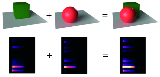
Figure 1: Illustration of the effects of opacity and occlusion in visual and auditory (spectral) domains.

2 Method

Given a mel-scale spectrogram representation $\mathbf{x}\in\mathbb{R}^{D_{in}\times h\times w}$ of a musical chord, our goal is to decompose it into its constituent note-level spectrograms $\mathbf{x}_{k}\in\mathbb{R}^{D_{in}\times h\times w}\quad\forall k=\{1,2,...,K\}$ and learn their associated representations (slots) $\mathbf{s}\in\mathbb{R}^{{D}_{s}\times K}$. Here, $D_{in}$ denotes the number of channels in the spectrogram, $D_{s}$ the slot size, $h,w$ the number of frequency bins and time window of the input spectrogram respectively and $K$ the total number of slots. Our proposed MusicSlots model is an autoencoder which consists of three modules (see Figure 2). An encoder module (CNN) to extract features from the input spectrogram, slot attention module to group input features to slots and decoder module to reconstruct the chord spectrogram from the slot representations.

Encoder.

The encoder module consists of a CNN backbone to extract features $\mathbf{h}\in\mathbb{R}^{{D}_{f}\times h\times w}$ from the input chord spectrogram $\mathbf{x}$. Learnable positional embeddings $\mathbf{p}\in\mathbb{R}^{D_{f}\times h\times w}$ (see Section A.2 for more details) are added to the output features $\mathbf{h}$ from the final convolutional layer.

Slot Attention.

The slot attention module learns to map a set of $N=h\cdot w$ input features onto a set of $K$ slots using an iterative attention mechanism (Algorithm 1 from Locatello et al. [19]) implemented via key-value attention [28] and recurrent update function. The input features $\mathbf{h}$ are projected to a set of keys $\mathbf{k}$ and values $\mathbf{v}\in\mathbb{R}^{D_{s}\times N}$ using separate linear layers. Each slot $s_{k}$ is initialized as independent samples from a Gaussian distribution $\mathcal{N}(\mu_{k},\sigma_{k})$ with separate learnable mean $\mu_{k}\in\mathbb{R}^{D_{s}}$ and standard-deviation $\sigma_{k}\in\mathbb{R}^{D_{s}}$. Then at each iteration $t=\{1,...,T\}$, slots compete to represent elements of the set of features using standard key-value attention (with features as keys & values and slots as queries) except with softmax normalization applied across the slots. We use a recurrent network (specifically a GRU [29, 30]) and residual MLP [19]) to update the slots with weighted values as inputs and slots at $t-1$ as hidden states of the RNN. Further, our MusicSlots model also adopts recent improvements to SlotAttention such as implicit differentiation [31].

Decoder.

Each slot $s_{k}$ is decoded independently by the spatial broadcast decoder [32] (see Figure 2) using several de-convolutional layers. First, slots are broadcasted onto a 2D grid (independently) and learnable positional embeddings are added. The decoder outputs the reconstructed note-level spectrogram $\mathbf{\hat{x}}_{k}\in\mathbb{R}^{D_{in}\times h\times w}$ and un-normalized (logits) alpha mask $\mathbf{m}_{k}\in\mathbb{R}^{1\times h\times w}$. The individual slot-wise spectrograms and normalized masks $\mathbf{\overline{m}}_{k}=f_{norm}(\mathbf{m}_{k})\in\mathbb{R}^{1\times h\times w}$ are alpha composited to give the predicted power-scale chord spectrogram $\mathbf{\hat{x}}_{p}=\sum_{k=1}^{K}\mathbf{\hat{p}}_{k}\odot\mathbf{\overline{m}}_{k}$ where $\mathbf{\hat{p}}_{k}$ is the power-scale note spectrogram, $\odot$ is an element-wise multiplication and $f_{norm}$ is the normalization function. This composition operation needs to carried out in power-scale followed by conversion back to decibel scale to get the predicted chord spectrogram $\mathbf{\hat{x}}$ as follows:

$$\mathbf{\hat{p}}_{k}=10^{\mathbf{\hat{x}}_{k}/10}\quad;\quad\mathbf{\hat{x}}_{p}=\sum_{k=1}^{K}\mathbf{\hat{p}}_{k}\odot\mathbf{\overline{m}}_{k}\quad;\quad\mathbf{\hat{x}}=10\log_{10}\Big{(}\frac{\mathbf{\hat{x}}_{p}}{\mathbf{\hat{x}}_{p0}}\Big{)}\textrm{dB}$$ (1)

where $\mathbf{\hat{p}}_{k}$ is the power-scale note spectrogram, $\mathbf{x}_{p}$ is the chord spectrogram in power scale and $\mathbf{\hat{x}}_{p0}$ is the reference power. Further, a crucial modification required to adapt SlotAttention to the audio domain, is the choice of this normalization function $f_{norm}$ for alpha masks. For auditory objects, as illustrated in Figure 1 notions of occlusion and opacity are invalid which means that its feasible for one or more notes (slots) to contribute to the power at a spatial location (frequency bin and time) in the spectrogram. Contrarily, in the visual domain its necessarily the case that every pixel belongs to only one object. Therefore, we experiment with alternatives such as Sigmoid and not using any alpha masks in the broadcast decoder. We train our MusicSlots model using the MSE between the predicted and input chord spectrogram $\mathcal{L}=||\mathbf{x}-\mathbf{\hat{x}}||_{2}^{2}$. For more details on model architecture and training hyperparameters please refer to Section A.2 and Section A.3 respectively.

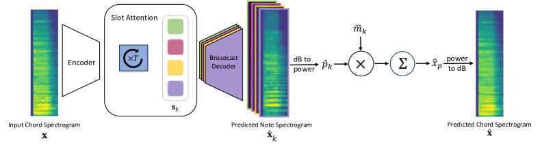
Figure 2: MusicSlots model consists of 3 modules — Encoder, SlotAttention and Broadcast Decoder.

3 Related Work

Learning music representations from audio has been explored using self-supervised techniques such as autoencoders [33, 34, 35] and contrastive methods [36, 37, 38, 39] or weak supervision from different modalities [40, 41, 42, 43]. Related to our work, ‘Audioslots’ [44] applies object-centric models to the audio domain for blind source separation. However, their model is strongly supervised as it is trained using MSE loss between predicted and matched ground-truth individual source spectrograms. Others have applied slot-based object-centric models beyond vision to learn modular action sequences for RL agents [45] or robotic control policies [46].

4 Results

We describe details of our multi-object music dataset followed by results on unsupervised note discovery and supervised note property prediction tasks.

Multi-Object Music Datasets.

To evaluate the efficacy of our proposed MusicSlots model on the unsupervised music decomposition task, we need a dataset of musical scores in the spectral format and its decomposition into sub-parts i.e. part-level spectrograms and binary masks (see Figure 4). We introduce synthetic multi-object datasets to specifically evaluate object-centric learning methods on the music domain analogous to its visual counterpart [25]. First, we extract chords (MIDI tokens) from Bach-Chorales (JSB) [26] and JazzNet [27] datasets. Next, we synthesize the audio waveform and its spectrogram for these chords (see Section A.1 for more details). Our dataset consists of two variants — i) single-instrument: all notes in a chord played by the same instrument, ii) multi-instrument: different notes in a chord played by different instruments. We create out-of-distribution test splits that measure generalization to unseen note combinations and number of notes in a chord. The test split in Bach Chorales contains chords with known notes in unknown combinations (w.r.t train/validation splits) whereas in JazzNet it contains only chords with four notes, while training and validation splits consist of two and three-note chords (see Section A.1 for more details).

Note Discovery.

We train three variants of our MusicSlots model with different choices for $f_{norm}$ — i) Softmax (MusicSlots-soft) ii) Sigmoid (MusicSlots-sigm) iii) no alpha mask usage (MusicSlots-none). We refer to LABEL:table:_note_discovery_training and Section A.2 for model/training details. We quantitatively measure note (object) discovery performance of our models using the best matched note-level MSE of spectrograms and mean IoU scores of binary masks. Table 1 shows the note discovery results of MusicSlots on multi-instrument versions of JSB and JazzNet datasets. We see that the MusicSlots without any alpha masking is competitive with Sigmoid normalization and these alternatives show significant performance gains over the default Softmax. Further, we observe that training on multi-instrument chord datasets is beneficial for better decomposition quality (compare with single-instrument in Appendix B). We show samples of good decomposition and some failure cases of our MusicSlots model in Appendix C.

Table 1: Note discovery results on multi-instrument BachChorales (JSB) and JazzNet datasets for MusicSlots models. Mean and std-dev. are reported across 5 seeds.

Datasets Mask Norm. Note MSE $\downarrow$ mIoU $\uparrow$ JSB-multi MusicSlots-soft 59.34 ${\scriptstyle\pm 22.01}$ 0.79 ${\scriptstyle\pm 0.04}$ MusicSlots-sigm 13.07 ${\scriptstyle\pm 0.80}$ 0.90 ${\scriptstyle\pm 0.01}$ MusicSlots-none 13.47 ${\scriptstyle\pm 0.90}$ 0.91 ${\scriptstyle\pm 0.01}$ JazzNet-multi MusicSlots-soft 33.58 ${\scriptstyle\pm 2.08}$ 0.84 ${\scriptstyle\pm 0.01}$ MusicSlots-sigm 18.53 ${\scriptstyle\pm 0.83}$ 0.91 ${\scriptstyle\pm 0.01}$ MusicSlots-none 19.95 ${\scriptstyle\pm 1.89}$ 0.90 ${\scriptstyle\pm 0.01}$

Note Property Prediction.

We train a linear classifier with cross-entropy loss (see Section A.2 for details) to predict the properties (MIDI pitch value and instrument type) of all notes in a chord from the frozen (pre-trained) latent representations. We use the classification accuracy as the evaluation metric for this task wherein a chord is considered to be correctly classified if and only if all its note pitch values and instrument identities are correctly predicted. The supervised CNN baseline uses the same encoder module as MusicSlots followed by a two layer MLP and trained in a supervised manner to predict the note properties given the chord spectrogram. Table 2 shows the note property results for our MusicSlots model against various baseline models. We see that our MusicSlots model outperforms several unsupervised baseline models (AutoEncoder/VAE/$\beta$-VAE). Surprisingly it also outperforms the supervised CNN baseline which is explicitly trained end-to-end to solve the task. Further, MusicSlots shows a greater degree of generalization to unseen note combinations on the test splits of JSB-multi and different number of notes in a chord on JazzNet-multi respectively.

Table 2: Note property prediction performance of MusicSlots compared to Autoencoder, VAE, $\beta$-VAE and supervised CNN baseline models. Mean and std-dev. are reported across 5 seeds.

Models JSB-multi JazzNet-multi Val-Acc. Test-Acc. Val-Acc. Test-Acc. Supervised CNN 93.49 ${\scriptstyle\pm 2.10}$ 93.03 ${\scriptstyle\pm 2.10}$ 96.47 ${\scriptstyle\pm 0.79}$ 71.22 ${\scriptstyle\pm 2.93}$ AutoEncoder 95.02 ${\scriptstyle\pm 0.09}$ 93.62 ${\scriptstyle\pm 0.39}$ 92.91 ${\scriptstyle\pm 0.26}$ 71.37 ${\scriptstyle\pm 1.07}$ VAE 96.66 ${\scriptstyle\pm 0.34}$ 96.21 ${\scriptstyle\pm 0.35}$ 94.37 ${\scriptstyle\pm 0.55}$ 71.55 ${\scriptstyle\pm 4.77}$ $\beta$-VAE 97.85 ${\scriptstyle\pm 0.13}$ 97.42 ${\scriptstyle\pm 0.06}$ 97.00 ${\scriptstyle\pm 0.37}$ 81.53 ${\scriptstyle\pm 0.77}$ MusicSlots-none 98.13 ${\scriptstyle\pm 0.16}$ 97.77 ${\scriptstyle\pm 0.12}$ 98.96 ${\scriptstyle\pm 0.39}$ 87.65 ${\scriptstyle\pm 1.88}$

5 Conclusion

Our MusicSlots model is the first method to extend object-centric learning to the domain of music. To evaluate such models, we introduced novel multi-object music datasets based on Western tonal music. MusicSlots successfully decomposes chord spectrograms into their constituent note spectrograms, and outperforms several well-established unsupervised and supervised baselines on downstream note property prediction tasks. Representations learned by MusicSlots are potentially useful for practical applications, such as music transcription/generation and building more human-like perceptual models of audio and music.

Acknowledgments.

We thank Hamza Keurti and Yassine Taoudi Benchekroun for insightful discussions. This research was funded by Swiss National Science Foundation grant: 200021_192356, project NEUSYM and the ERC Advanced grant no: 742870, AlgoRNN. We also thank NVIDIA Corporation for donating DGX machines as part of the Pioneers of AI Research Award.

Appendix A Experimental Details

In this section, we report details on our multi-object music datasets, model implementation, and experimental setting.

A.1 Multi-Object Music Dataset

Bach Chorales.

The original dataset consists of training, validation and test splits with 229, 76 and 77 chorales respectively. Each chorale is represented as a sequence of four MIDI values for the Bass, Tenor, Alto and Soprano (BTAS) voices. If a voice is silent at a given time step, the pitch value is 0. Since we are interested in extracting unique chords from the chorales, we first concatenate all MIDI sequences of the 376 chorales together across time, and exclude all the columns corresponding to duplicate chords or single note examples, giving us 3131 unique chords in total. We then randomly shuffle the dataset and partition it into training, validation and test splits, using a train-validation-test split ratio of 70/20/10. The MIDI pitch values for the chorales are available at https://github.com/czhuang/JSB-Chorales-dataset.

JazzNet.

The JazzNet dataset (https://github.com/tosiron/jazznet) contains 5525 annotated chords (including the inversions). Of the 5525 chords, we use 2227 unique chords with the MIDI pitch values of their notes ranging from 36 (C2) to 96 (C7). Similar to the chords in the Bach Chorales, the pitch values of the JazzNet chords are represented as an array of 4 MIDI values, with 0 denoting silence. The train-validation-test splits are defined such that the training and validation sets contain only dyads (2-notes) and triads (3-notes), while the test set contains only tetrads (4-notes).

In the the following paragraphs we describe the details of the pipeline to generate our multi-object music datasets starting with the MIDI tokens of chords and finally getting chord/note-level spectrograms and binary masks.

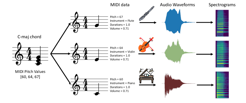
Figure 3: Multi-instrument dataset generation pipeline. Every note in the chord can be synthesized into a raw audio waveform using a different instrument (e.g. Yamaha grand piano, violin, flute).

MIDI File Generation.

To allow fine-grained control over the note properties, we generate the MIDI files for the chords ourselves using the Music21 library. Our data sources define the chords and their pitch values, and we specify the rest of their note attributes (i.e. volume, instrument, duration), as shown in Figure 3. In the Music21 library, the volume of the note is a scalar value ranging from 0.0 to 1.0 while the duration of the note is measured in seconds. We keep the duration and volume fixed across datasets by setting them to 0.71 and 1.0 second respectively. To generate examples for the multi-instrument version of our dataset, we include the option to change the instrument that plays each note in a chord. The list of instruments is defined by a sf2 file. The sf2 file that is used in our dataset can be downloaded here: https://member.keymusician.com/Member/FluidR3_GM/index.html.

Audio Waveform Generation.

The generated MIDI files are then synthesized into audio waveforms using Fluidsynth (https://www.fluidsynth.org/). The default PCM quantization settings used in the Fluidsynth library are bit-depth of 16 and sample rate of 44.1 kHz. We further downsample the waveforms to 16kHz. We zero-pad the waveforms at the start with a padding size of 4000, which corresponds to about 0.1s of silence.

Waveform to Spectrogram Conversion.

We obtain the spectrograms for the chords and their notes by converting their audio waveforms into mel-spectrograms using the TorchAudio library (https://pytorch.org/audio/stable/index.html). We set the number of mel-filter banks to 128 and use the FFT and window sizes of 1024 and hop length of 512. The resulting $128\times 35$ spectrogram is resized by cropping along the width boundaries [0, 32], giving us a resolution of $128\times 32$. To generate a chord spectrogram, we combine the waveforms of its constituent notes, and convert the summed waveform to a mel-spectrogram using the same mel-spectrogram parameters.

Mask Generation.

To generate the binary masks from the mel-spectrograms, we use a fixed decibel threshold value of -30 dB for both the ground-truth and the predicted note spectrograms. Examples of the binary masks for different note spectrograms are shown in Figure 4.

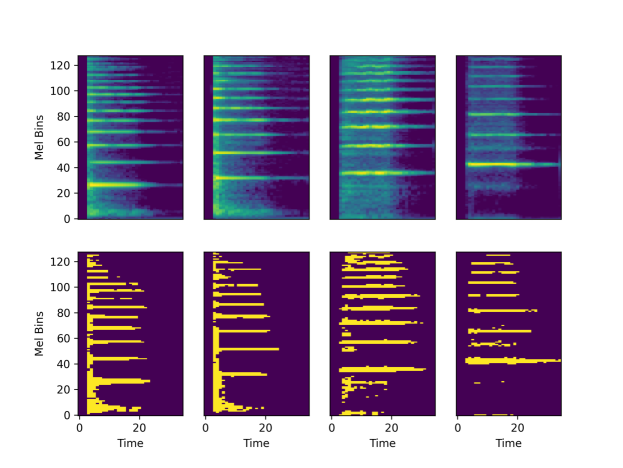
Figure 4: Visualization of the note spectrograms (top row) and the corresponding decibel-thresholded binary masks (bottom row)

Dataset Statistics.

In Tables 3 and 4, we report the numbers of dyads, triads and tetrads in the datasets. The dataset splits, number of unique pitch values (represented as MIDI note numbers) and instruments are summarized in Table 5.

Table 3: Chord statistics for Bach Chorales.

Splits	Dyads	Triads	Tetrads	Total
Train	10	270	1910	2190
Validation	1	85	540	626
Test	1	43	271	315
Total	12	398	2721	3131

Table 4: Chord statistics for JazzNet

Splits	Dyads	Triads	Tetrads	Total
Train	530	544	0	1074
Validation	124	145	0	269
Test	0	0	884	884
Total	654	689	884	2227

Table 5: Number of examples in the dataset splits, number of unique pitch values and name of the instruments used.

Dataset Name	Train	Validation	Test	Pitch Values	Instrument(s)
JSB-single	2190	626	315	53	Piano
JSB-multi	19719	5634	2826	53	Piano, Violin, Flute
Jazznet-single	1074	269	884	62	Piano
Jazznet-multi	19458	5031	71604	62	Piano, Violin, Flute

A.2 Model Architecture Details

Here we describe the architectural details of all models used in this work.

Convolutional Encoder.

Table 6 describes the model architecture for the CNN encoder of the MusicSlots. We use a CNN encoder similar to the one found in [19] for the unsupervised object discovery task. All convolution layers use a kernel size of $5\times 5$ with a channel size of 128. Unlike [19], we set the stride for the horizontal axis to 2. We find that this improves performance for the unsupervised note discovery task (see Table 15 for details).

Table 6: CNN Encoder in MusicSlots.

Layer	Feature Dimension $H\times W\times C$	Activation	Stride	Padding Input / Output
Input	$128\times 32\times 1$	-	-	-
Conv $5\times 5$	$128\times 16\times 128$	ReLU	(1, 2)	(2, 2) / -
Conv $5\times 5$	$128\times 8\times 128$	ReLU	(1, 2)	(2, 2) / -
Conv $5\times 5$	$128\times 4\times 128$	ReLU	(1, 2)	(2, 2) / -
Conv $5\times 5$	$128\times 2\times 128$	ReLU	(1, 2)	(2, 2) / -
Position Embedding	$128\times 2\times 128$	-	-	-
Flatten	$1\times 256\times 128$	-	-	-
Layer Norm	$1\times 256\times 128$	-	-	-
Linear	$1\times 256\times 128$	ReLU	-	-
Linear	$1\times 256\times 128$	-	-	-

Positional Embedding.

We use the same positional embeddings as [19]. The positional embedding is a $W\times H\times 4$ tensor, where $W$ and $H$ are width and height of the CNN feature maps respectively. The positional information is defined by a linear gradient [0, 1] in each of the four cardinal directions. Essentially, every point on the grid is a four-dimensional vector that indicates its relative distance to the four edges of the feature map. We define a learnable linear projection that projects the feature vectors to match the dimensionality of the CNN feature vectors. We finally add the linearly projected result to the input CNN feature maps.

Slot Attention Module.

For all experiments, we use the same number of slots $K=7$ and slot attention iterations $T=3$. We set $D$ and $D_{s}$ to be 128 for the dimensions of the linear projections and the slots respectively. The hidden state of the GRU cell has a dimension of 128. The residual MLP has a single hidden layer of size 128 with ReLU activation, followed by a linear layer.

De-convolutional Decoder.

We follow the same spatial broadcast deconvolutional decoder ([32]) used in [19], except we set the number of channels in the transposed convolution layers to 128. The overall architecture for the MusicSlots decoder is detailed in Table 7.

Table 7: Deconvolution-based slot decoder in MusicSlots.

Layer	Feature Dimensions $K\times H\times W\times C$	Activation	Stride	Padding Input / Output
Input	$7\times 1\times 1\times 128$	-	-	-
Spatial Broadcast	$7\times 8\times 2\times 128$	-	-	-
Position Embedding	$7\times 8\times 2\times 128$	-	-	-
ConvTranspose $5\times 5$	$7\times 16\times 4\times 128$	ReLU	(2, 2)	(2, 2) / (1, 1)
ConvTranspose $5\times 5$	$7\times 32\times 8\times 128$	ReLU	(2, 2)	(2, 2) / (1, 1)
ConvTranspose $5\times 5$	$7\times 64\times 16\times 128$	ReLU	(2, 2)	(2, 2) / (1, 1)
ConvTranspose $5\times 5$	$7\times 128\times 32\times 128$	ReLU	(2, 2)	(2, 2) / (1, 1)
ConvTranspose $5\times 5$	$7\times 128\times 32\times 128$	ReLU	(1, 1)	(2, 2) / -
ConvTranspose $3\times 3$	$7\times 128\times 32\times 1$	-	(1, 1)	(1, 1) / -

Baseline AutoEncoders.

The architectural details for the encoder and decoder of the baseline AutoEncoders (AutoEncoder, VAE, $\beta$-VAE) are presented in Tables 8 and 9. We set the latent space dimension for the baseline AutoEncoders to 128.

Table 8: Convolutional encoder for the baseline AutoEncoders, excluding the final two Linear layers that parameterize the $\mu$ and $\sigma$ of the approximate posterior for the VAE.

Layer	Feature Dimension $H\times W\times C$	Activation	Stride	Padding Input / Output
Input	$128\times 32\times 1$	-	-	-
Conv $5\times 5$	$64\times 16\times 128$	ReLU	(2, 2)	(2, 2) / -
Conv $5\times 5$	$32\times 8\times 128$	ReLU	(2, 2)	(2, 2) / -
Conv $5\times 5$	$16\times 4\times 128$	ReLU	(2, 2)	(2, 2) / -
Conv $5\times 5$	$8\times 2\times 128$	ReLU	(2, 2)	(2, 2) / -
Flatten	$1\times 1\times 2048$	-	-	-

Table 9: De-convolutional decoder for the AutoEncoder baselines.

Layer	Feature Dimensions $H\times W\times C$	Activation	Stride	Padding Input / Output
Input	$1\times 1\times 128$	-	-	-
Linear	$1\times 1\times 2048$	-	-	-
Reshape	$8\times 2\times 128$	-	-	-
ConvTranspose $5\times 5$	$16\times 4\times 128$	ReLU	(2, 2)	(2, 2) / (1, 1)
ConvTranspose $5\times 5$	$32\times 8\times 128$	ReLU	(2, 2)	(2, 2) / (1, 1)
ConvTranspose $5\times 5$	$64\times 16\times 128$	ReLU	(2, 2)	(2, 2) / (1, 1)
ConvTranspose $5\times 5$	$128\times 32\times 128$	ReLU	(2, 2)	(2, 2) / (1, 1)
ConvTranspose $5\times 5$	$128\times 32\times 128$	ReLU	(1, 1)	(2, 2) / -
ConvTranspose $3\times 3$	$128\times 32\times 1$	-	(1, 1)	(1, 1) / -

Linear Classifier for MusicSlots.

A linear classifier is trained on every slot that is matched with a note to independently predict its pitch value and instrument identity. The linear classifier outputs two vectors $\hat{y}_{\text{inst}}\in N_{\text{inst}}$ and $\hat{y}_{\text{pitch}}\in N_{\text{pitch}}$, where $N_{\text{pitch}}$ is the number of unique pitch values and $N_{\text{inst}}$ is the number of instruments in the dataset. Both $\hat{y}_{\text{inst}}$ and $\hat{y}_{\text{pitch}}$ are normalized using a softmax activation, since pitch values and instrument identities are encoded as one-hot vectors.

Linear Classifier for Baseline AutoEncoders.

In the baseline AutoEncoders, the representations of individual notes are not readily available. Therefore, the input to the linear classifier is a single latent vector. The classifier outputs a prediction $\hat{y}\in N_{\text{inst}}\times N_{\text{pitch}}$ for the properties of all the notes in a chord at once. In this case, $\hat{y}$ uses sigmoid activation, since the label $y$ is encoded as a multi-hot vector.

Supervised CNN.

The model architecture for the supervised baseline CNN is depicted in Table 10. It follows the same encoder backbone as the one used in MusicSlots. The output of the encoder module is followed by a 2-layer MLP with an output size $N_{\text{inst}}\times N_{\text{pitch}}$.

Table 10: Supervised CNN for the property prediction task.

Layer	Feature Dimension $H\times W\times C$	Activation	Stride	Padding Input / Output
Input	$128\times 32\times 1$	-	-	-
Conv $5\times 5$	$64\times 16\times 128$	ReLU	(2, 2)	(2, 2) / -
Conv $5\times 5$	$32\times 8\times 128$	ReLU	(2, 2)	(2, 2) / -
Conv $5\times 5$	$16\times 4\times 128$	ReLU	(2, 2)	(2, 2) / -
Conv $5\times 5$	$8\times 2\times 128$	ReLU	(2, 2)	(2, 2) / -
Flatten	$1\times 1\times 2048$	-	-	-
Linear	$1\times 1\times 128$	ReLU	-	-
Linear	$1\times\text{output size}$	Sigmoid	-	-

A.3 Training Details

In this section, we provide an overview of the training details for MusicSlots and its baselines, including their hyperparameter choices and training objectives. The hyperparameters for training MusicSlots on the unsupervised note discovery task are shown in Table LABEL:table:_note_discovery_training. All downstream classifiers, including the supervised CNN model, share the common hyperparameters for the note property prediction task, as shown in Table LABEL:table:_note_property_training. The training hyperparameters for the unsupervised baselines (i.e. AutoEncoder, VAE, $\beta$-VAE) are displayed in Table 13.

Baseline AutoEncoders.

The baseline AutoEncoder follows the same training objective as MusicSlots: they are both trained to minimize the Mean Square Error (MSE) between the predicted and input chord spectrogram $\mathcal{L}=||\mathbf{x}-\mathbf{\hat{x}}||_{2}^{2}$. The baseline VAE and $\beta$-VAE models are trained by maximizing the evidence lower bound (ELBO), where the weight of the KL-divergence term $\beta$ is set to 1 for the baseline VAE. For more details on the effect of different choices for $\beta$ on the downstream note property prediction task, please refer to Table 16 in Appendix B.

Downstream Classifiers.

The downstream note property classifier for MusicSlots is trained by minimizing the categorical cross-entropy loss. For the supervised CNN and the linear classifier trained on the baseline AutoEncoders, we use binary cross-entropy loss, since the target is a multi-hot vector.

Table 11: Training hyperparameters of the MusicSlots model for unsupervised note discovery experiments

Hyperparameters
Training Steps	100K
Batch Size	32
Optimizer	Adam
Max. Learning Rate	1e-04
Learning Rate Warmup Steps	10K
Decay Steps	500K
Gradient Norm Clipping	1.0

Table 12: Training hyperparameters for the note property prediction task

Hyperparameters
Training steps	10K
Batch Size	32
Optimizer	Adam
Learning Rate	1e-03

Table 13: Training hyperparameters for the baseline AEs during the unsupervised pre-training.

Hyperparameters
Training Steps	100K
Learning Rate	1e-04
Batch Size	32
Optimizer	Adam
Decay Steps	100K
Gradient Norm Clipping	1.0

A.4 Evaluation Details

Note Discovery.

To compute the note MSE, we first calculate the mean squared error between all pairs of predicted and ground-truth note spectrograms. Since the orders of the predictions and the ground-truth are arbitrary, we match them using the Hungarian algorithm ([47]) to find the matching with the lowest MSE. mIoU is calculated by first computing all pairwise IoUs between the predicted and ground-truth dB-thresholded masks, and using the Hungarian algorithm to find the optimal assignment that gives the highest mIoU. For the Hungarian matching algorithm, we use the scipy implementation scipy.optimize.linear_sum_assignment.

Note Property Prediction.

The performance of the classifiers is quantified using classification accuracy. The accuracy is measured by computing the percentage of correctly classified chord examples in the dataset. A chord is considered to be correctly classified if and only if the classifier predictions for all of its note properties (i.e. note pitch values, instrument identities) are correct.

Appendix B Additional Results

In this section, we present additional results that quantify the importance of different modelling choices.

Single-instrument Note Discovery Results

Table 14 shows the unsupervised note discovery performance of our MusicSlots model with different alpha mask normalization choices on the single-instrument JSB and JazzNet datasets. We observe significant performance gain in the single-instrument setting when sigmoid-normalized alpha masks or no alpha masks are used in our MusicSlots model.

Table 14: Note discovery results on single-instrument BachChorales (JSB) and JazzNet datasets for MusicSlots models with different choices for $f_{norm}$ function. Mean and std-dev. are reported across 5 seeds.

Datasets Mask Norm. Note MSE $\downarrow$ mIoU $\uparrow$ JSB-single MusicSlots-soft 75.32 ${\scriptstyle\pm 37.63}$ 0.68 ${\scriptstyle\pm 0.08}$ MusicSlots-sigm 18.21 ${\scriptstyle\pm 3.40}$ 0.83 ${\scriptstyle\pm 0.02}$ MusicSlots-none 22.44 ${\scriptstyle\pm 7.07}$ 0.81 ${\scriptstyle\pm 0.03}$ JazzNet-single MusicSlots-soft 114.09 ${\scriptstyle\pm 22.72}$ 0.63 ${\scriptstyle\pm 0.04}$ MusicSlots-sigm 49.05 ${\scriptstyle\pm 5.98}$ 0.75 ${\scriptstyle\pm 0.03}$ MusicSlots-none 44.49 ${\scriptstyle\pm 0.62}$ 0.76 ${\scriptstyle\pm 0.02}$

Ablation on Architectural Modifications

Table 15 presents our ablation study on different architectural choices in our MusicSlots model on the multi-instrument Bach Chorales and JazzNet datasets. We start from the ‘Default’ model that follows the same setup used for object discovery in [19]. In this setup, we have stride length of (1, 1) in the convolutional encoder layers and the alpha masks of the decoder are normalized using the Softmax function. We find that both implicit differentiation ([31]) and the removal of the alpha masks from the decoder play a crucial role in improving the note discovery performance of our MusicSlots model. Increasing the stride length along the time axis to 2 also improves its performance, though not as significantly as the other two design choices. By combining these improvements in the model architecture and training optimization, we finally arrive at our MusicSlots model without any alpha masking.

Table 15: Architectural ablations on the MusicSlots for unsupervisd note discovery task. ‘Default’ here refers to the MusicSlots model with the setup used for object discovery in [19] , where stride = (1, 1) in the convolutional encoder layers and the spatial broadcast decoder outputs softmax alpha masks.

Dataset	Model	Note MSE $\downarrow$	mIoU $\uparrow$
JazzNet-multi	Default	70.05 $\scriptstyle{\pm 23.61}$	0.70 $\scriptstyle{\pm 0.07}$
	Default + stride_length = (1, 2)	51.31 $\scriptstyle{\pm 1.89}$	0.76 $\scriptstyle{\pm 0.04}$
	Default - Softmax Alpha Mask	39.08 $\scriptstyle{\pm 6.35}$	0.79 $\scriptstyle{\pm 0.02}$
	Default + Implicit Differentiation	32.56 $\scriptstyle{\pm 9.84}$	0.83 $\scriptstyle{\pm 0.00}$
	MusicSlots	19.95 $\scriptstyle{\pm 1.89}$	0.90 $\scriptstyle{\pm 0.01}$
JSB-multi	Default	100.77 $\scriptstyle{\pm 52.91}$	0.60 $\scriptstyle{\pm 0.15}$
	Default + stride_length = (1, 2)	60.22 $\scriptstyle{\pm 14.56}$	0.76 $\scriptstyle{\pm 0.04}$
	Default - Softmax Alpha Mask	40.06 $\scriptstyle{\pm 14.60}$	0.78 $\scriptstyle{\pm 0.04}$
	Default + Implicit Differentiation	59.34 $\scriptstyle{\pm 22.01}$	0.79 $\scriptstyle{\pm 0.04}$
	MusicSlots	13.47 $\scriptstyle{\pm 0.90}$	0.91 $\scriptstyle{\pm 0.01}$

VAE Ablation

Table 16 shows the ablation study for the choice of $\beta$ in the VAEs on the multi-instrument Bach Chorales and JazzNet datasets. We observe that higher $\beta$ results in worse downstream property prediction performance on both datasets and the best results are achieved using $\beta=0.5$.

Table 16: Note property prediction performance of baseline VAEs with different $\beta$ values. $\beta=1$ corresponds to the vanilla VAE model. As we increase $\beta$, the property prediction performance using the latent representations from the $\beta$-VAE worsens on both JSB and Jazznet multi-instrument datasets.

$\beta$	JSB-multi		Jazznet-multi
	Val-Acc.	Test-Acc.	Val-Acc.	Test-Acc.
0.5	97.85 ${\scriptstyle\pm 0.13}$	97.42 ${\scriptstyle\pm 0.06}$	97.00 ${\scriptstyle\pm 0.38}$	81.53 ${\scriptstyle\pm 0.77}$
1.0	96.66 ${\scriptstyle\pm 0.34}$	96.21 ${\scriptstyle\pm 0.35}$	94.37 ${\scriptstyle\pm 0.55}$	71.55 ${\scriptstyle\pm 4.77}$
2.0	92.23 ${\scriptstyle\pm 0.66}$	90.74 ${\scriptstyle\pm 0.94}$	73.93 ${\scriptstyle\pm 1.97}$	47.90 ${\scriptstyle\pm 8.59}$
4.0	82.07 ${\scriptstyle\pm 0.83}$	78.95 ${\scriptstyle\pm 1.42}$	47.51 ${\scriptstyle\pm 3.71}$	11.31 ${\scriptstyle\pm 1.92}$

Appendix C Note Discovery Visualization

We provide additional visualization samples of note discovery results from our MusicSlots model on the JazzNet and Bach Chorales datasets, including both the success and failure cases. We also visualize the effect of using Softmax alpha masks in MusicSlots for note discovery in Figure 11.

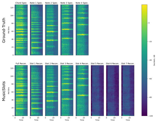
Figure 5: Unsupervised note discovery result on the JSB-multi-instrument dataset. The MusicSlots accurately predicts the ground-truth note spectrograms. It also learns to capture the background (i.e. silence) in the remaining slots that are not matched with the ground-truth notes.

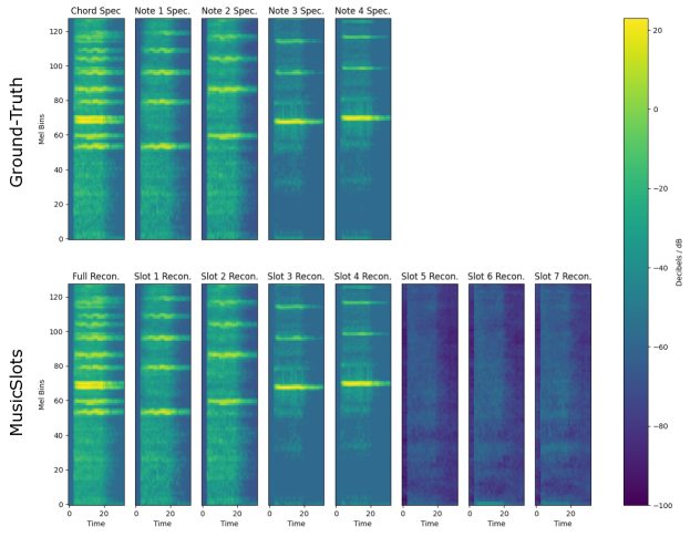
Figure 6: Unsupervised note discovery result on the Jazznet-multi-instrument dataset. Similar to the example visualized in Figure 5, MusicSlots successfuly decomposes the given chord spectrogram into its constituent note spectrograms and distribute the background across the remaining slots.

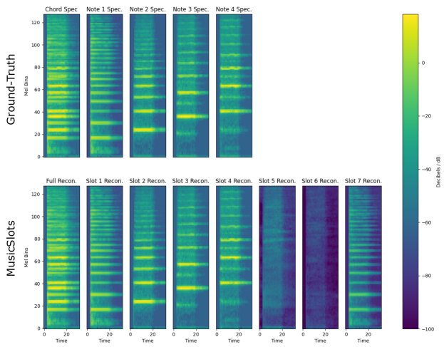
Figure 7: Unsupervised note discovery result on the JSB-multi-instrument dataset. On this example, MusicSlots successfully predicts most of the ground-truth note spectrograms. However, it oversegments one of the notes (Note 1) by assigning it to slot 1 and 7.

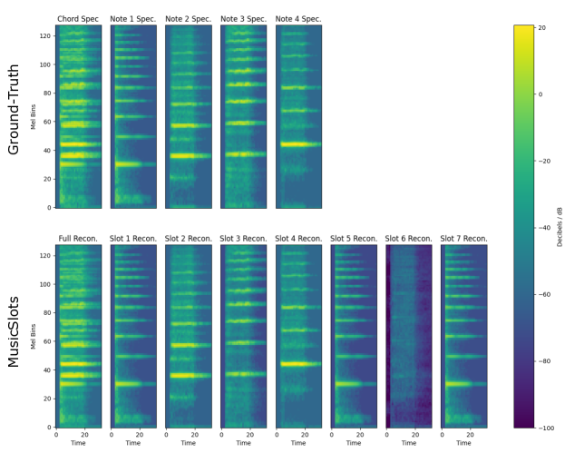
Figure 8: Unsupervised note discovery result on the JazzNet-multi-instrument dataset. Similar to the example shown in Figure 7, MusicSlots performs oversegmentation by using three slots (slot 1, 5 and 7) to model note 1.

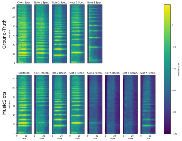
Figure 9: Visualization of a failure case of MusicSlots on the JSB-multi-instrument dataset. Only two of the four matched predictions accurately capture the harmonic structure of the ground-truth note spectrograms.

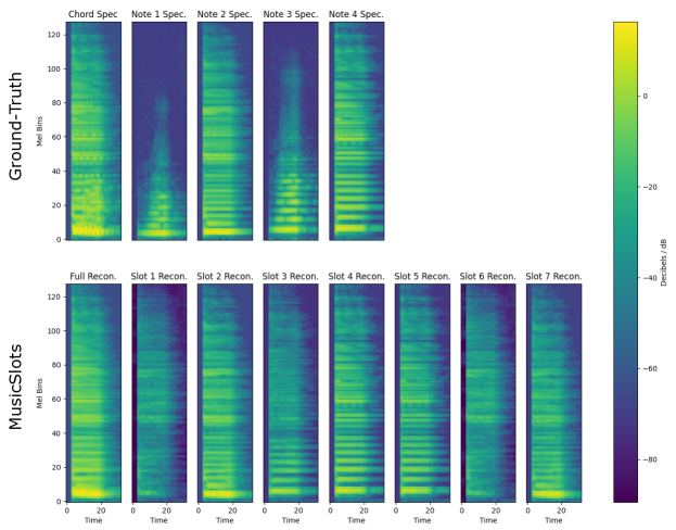
Figure 10: Visualization of a failure case of MusicSlots on the Jazznet-multi-instrument dataset. MusicSlots completely fails to predict notes 1 and 3 in its slot reconstructions. It also fails to model the background in any of the slots.

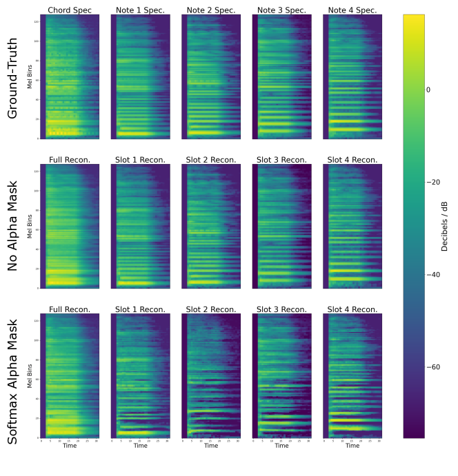
Figure 11: Qualitative performance comparison of MusicSlots without alpha masks (row 2) and MusicSlots with softmax-normalized alpha masks (row 3) on the JazzNet single-instrument dataset. MusicSlots with softmax alpha masks leaves unnatural gaps in the lower frequency bins where there is a strong degree of overlap between the note spectrograms. MusicSlots without any alpha mask does not introduce these artifacts and models the overlapping regions more accurately than its softmax normalized counterpart.

References

- Spelke [1990] Elizabeth S. Spelke. Principles of object perception. Cognitive Science, 14(1):29–56, 1990.
- Koffka [1935] Kurt Koffka. Principles of gestalt psychology. Philosophy and Scientific Method, 32(8), 1935.
- Köhler [1967] Wolfgang Köhler. Gestalt psychology. Psychologische Forschung, 31(1), 1967.
- Kubovy and Van Valkenburg [2001] Michael Kubovy and David Van Valkenburg. Auditory and visual objects. Cognition, 80(1-2):97–126, 2001.
- Griffiths and Warren [2004] Timothy D. Griffiths and Jason D. Warren. What is an auditory object? Nature Reviews Neuroscience, 5:887–892, 2004.
- Bizley and Cohen [2013] Jennifer K. Bizley and Yale E. Cohen. The what, where and how of auditory-object perception. Nature Reviews Neuroscience, 14:693–707, 2013.
- Kahneman et al. [1992] Daniel Kahneman, Anne Treisman, and Brian J Gibbs. The reviewing of object files: Object-specific integration of information. Cognitive psychology, 24(2):175–219, 1992.
- Hall et al. [2000] Michael D Hall, Richard E Pastore, Barbara E Acker, and Wenyi Huang. Evidence for auditory feature integration with spatially distributed items. Perception & Psychophysics, 62(6):1243–1257, 2000.
- Zmigrod and Hommel [2009] Sharon Zmigrod and Bernhard Hommel. Auditory event files: Integrating auditory perception and action planning. Attention, Perception, & Psychophysics, 71:352–362, 2009.
- Eslami et al. [2016] SM Ali Eslami, Nicolas Heess, Theophane Weber, Yuval Tassa, David Szepesvari, Geoffrey E Hinton, et al. Attend, infer, repeat: Fast scene understanding with generative models. In Proc. Advances in Neural Information Processing Systems (NIPS), pages 3225–3233, 2016.
- Greff et al. [2016] Klaus Greff, Antti Rasmus, Mathias Berglund, Tele Hao, Harri Valpola, and Jürgen Schmidhuber. Tagger: Deep unsupervised perceptual grouping. In Proc. Advances in Neural Information Processing Systems (NIPS), volume 29, 2016.
- Greff et al. [2017] Klaus Greff, Sjoerd van Steenkiste, and Jürgen Schmidhuber. Neural expectation maximization. In Proc. Advances in Neural Information Processing Systems (NIPS), pages 6691–6701, 2017.
- van Steenkiste et al. [2018] Sjoerd van Steenkiste, Michael Chang, Klaus Greff, and Jürgen Schmidhuber. Relational neural expectation maximization: Unsupervised discovery of objects and their interactions. In Int. Conf. on Learning Representations (ICLR), 2018.
- Kosiorek et al. [2018] Adam Kosiorek, Hyunjik Kim, Yee Whye Teh, and Ingmar Posner. Sequential attend, infer, repeat: Generative modelling of moving objects. In Proc. Advances in Neural Information Processing Systems (NIPS), pages 8606–8616, 2018.
- Stanić and Schmidhuber [2019] Aleksandar Stanić and Jürgen Schmidhuber. R-sqair: Relational sequential attend, infer, repeat. In Neurips Workshop on Perception as Generative Reasoning: Structure, Causality, Probability, 2019.
- Crawford and Pineau [2019] Eric Crawford and Joelle Pineau. Spatially invariant unsupervised object detection with convolutional neural networks. In Proc. AAAI Conf. on Artificial Intelligence, 2019.
- Burgess et al. [2019] Christopher P Burgess, Loic Matthey, Nicholas Watters, Rishabh Kabra, Irina Higgins, Matt Botvinick, and Alexander Lerchner. Monet: Unsupervised scene decomposition and representation. arXiv preprint arXiv:1901.11390, 2019.
- Greff et al. [2019] Klaus Greff, Raphaël Lopez Kaufman, Rishabh Kabra, Nick Watters, Christopher Burgess, Daniel Zoran, Loic Matthey, Matthew Botvinick, and Alexander Lerchner. Multi-object representation learning with iterative variational inference. In Proc. Int. Conf. on Machine Learning (ICML), pages 2424–2433, 2019.
- Locatello et al. [2020] Francesco Locatello, Dirk Weissenborn, Thomas Unterthiner, Aravindh Mahendran, Georg Heigold, Jakob Uszkoreit, Alexey Dosovitskiy, and Thomas Kipf. Object-centric learning with slot attention. In Proc. Advances in Neural Information Processing Systems (NeurIPS), 2020.
- Engelcke et al. [2020] Martin Engelcke, Adam R. Kosiorek, Oiwi Parker Jones, and Ingmar Posner. Genesis: Generative scene inference and sampling with object-centric latent representations. In Int. Conf. on Learning Representations (ICLR), 2020.
- Lin et al. [2020] Zhixuan Lin, Yi-Fu Wu, Skand Vishwanath Peri, Weihao Sun, Gautam Singh, Fei Deng, Jindong Jiang, and Sungjin Ahn. SPACE: unsupervised object-oriented scene representation via spatial attention and decomposition. In Int. Conf. on Learning Representations (ICLR), 2020.
- Singh et al. [2022] Gautam Singh, Fei Deng, and Sungjin Ahn. Illiterate DALLE learns to compose. In Int. Conf. on Learning Representations (ICLR), 2022.
- Kipf et al. [2022] Thomas Kipf, Gamaleldin Fathy Elsayed, Aravindh Mahendran, Austin Stone, Sara Sabour, Georg Heigold, Rico Jonschkowski, Alexey Dosovitskiy, and Klaus Greff. Conditional object-centric learning from video. In Int. Conf. on Learning Representations (ICLR), 2022.
- Lerdahl and Jackendoff [1983] Fred Lerdahl and Ray S Jackendoff. A Generative Theory of Tonal Music. MIT press, 1983.
- Kabra et al. [2019] Rishabh Kabra, Chris Burgess, Loic Matthey, Raphael Lopez Kaufman, Klaus Greff, Malcolm Reynolds, and Alexander Lerchner. Multi-object datasets. https://github.com/deepmind/multi-object-datasets/, 2019.
- Boulanger-Lewandowski et al. [2012] Nicolas Boulanger-Lewandowski, Yoshua Bengio, and Pascal Vincent. Modeling temporal dependencies in high-dimensional sequences: Application to polyphonic music generation and transcription. In Proc. Int. Conf. on Machine Learning (ICML), page 1881–1888, 2012.
- Adegbija [2023] Tosiron Adegbija. jazznet: A dataset of fundamental piano patterns for music audio machine learning research. In IEEE International Conference on Acoustics, Speech and Signal Processing (ICASSP), 2023.
- Vaswani et al. [2017] Ashish Vaswani, Noam Shazeer, Niki Parmar, Jakob Uszkoreit, Llion Jones, Aidan N Gomez, Łukasz Kaiser, and Illia Polosukhin. Attention is all you need. In Proc. Advances in Neural Information Processing Systems (NIPS), pages 5998–6008, 2017.
- Cho et al. [2014] Kyunghyun Cho, Bart van Merrienboer, Çaglar Gülçehre, Dzmitry Bahdanau, Fethi Bougares, Holger Schwenk, and Yoshua Bengio. Learning phrase representations using rnn encoder–decoder for statistical machine translation. In Proc. Conf. on Empirical Methods in Natural Language Processing (EMNLP), 2014.
- Gers et al. [2000] Felix A. Gers, Jürgen Schmidhuber, and Fred Cummins. Learning to Forget: Continual Prediction with LSTM. Neural Computation, 12(10):2451–2471, 2000.
- Chang et al. [2022] Michael Chang, Tom Griffiths, and Sergey Levine. Object representations as fixed points: Training iterative refinement algorithms with implicit differentiation. In Proc. Advances in Neural Information Processing Systems (NeurIPS), volume 35, pages 32694–32708, 2022.
- Watters et al. [2019] Nicholas Watters, Loic Matthey, Christopher P Burgess, and Alexander Lerchner. Spatial broadcast decoder: A simple architecture for learning disentangled representations in VAEs. In Learning from Limited Labeled Data (LLD) Workshop, ICLR, 2019.
- Caillon and Esling [2022] Antoine Caillon and Philippe Esling. RAVE: A variational autoencoder for fast and high-quality neural audio synthesis, 2022.
- Zeghidour et al. [2021] Neil Zeghidour, Alejandro Luebs, Ahmed Omran, Jan Skoglund, and Marco Tagliasacchi. Soundstream: An end-to-end neural audio codec. IEEE/ACM Transactions on Audio, Speech, and Language Processing, 30:495–507, 2021.
- Li et al. [2022] Yizhi Li, Ruibin Yuan, Ge Zhang, Yinghao Ma, Chenghua Lin, Xingran Chen, Anton Ragni, Hanzhi Yin, Zhijie Hu, Haoyu He, Emmanouil Benetos, Norbert Gyenge, Ruibo Liu, and Jie Fu. Map-music2vec: A simple and effective baseline for self-supervised music audio representation learning. In Proc. International Society for Music Information Retrieval, 2022.
- Spijkervet and Burgoyne [2021] Janne Spijkervet and John Ashley Burgoyne. Contrastive learning of musical representations. In Proc. International Society for Music Information Retrieval, 2021.
- McCallum et al. [2022] Matthew C. McCallum, Filip Korzeniowski, Sergio Oramas, Fabien Gouyon, and Andreas F. Ehmann. Supervised and unsupervised learning of audio representations for music understanding. In Proc. International Society for Music Information Retrieval, 2022.
- Choi et al. [2022] J. Choi, S. Jang, H. Cho, and S. Chung. Towards proper contrastive self-supervised learning strategies for music audio representation. In IEEE International Conference on Multimedia and Expo (ICME), pages 1–6, 2022.
- Wang et al. [2022] Luyu Wang, Pauline Luc, Yan Wu, Adria Recasens, Lucas Smaira, Andrew Brock, Andrew Jaegle, Jean-Baptiste Alayrac, Sander Dieleman, Joao Carreira, and Aaron van den Oord. Towards learning universal audio representations. In IEEE International Conference on Acoustics, Speech and Signal Processing (ICASSP), pages 4593–4597, 2022.
- Weston et al. [2011] Jason Weston, Samy Bengio, and Philippe Hamel. Multi-tasking with joint semantic spaces for large-scale music annotation and retrieval. Journal of New Music Research, 40(4):337–348, 2011.
- Park et al. [2017] Jiyoung Park, Jongpil Lee, Jangyeon Park, Jung-Woo Ha, and Juhan Nam. Representation learning of music using artist labels. In Proc. International Society for Music Information Retrieval, 2017.
- Manco et al. [2022] Ilaria Manco, Emmanouil Benetos, Elio Quinton, and György Fazekas. Learning music audio representations via weak language supervision. In IEEE International Conference on Acoustics, Speech and Signal Processing (ICASSP), pages 456–460, 2022.
- Chen et al. [2022] Tianyu Chen, Yuan Xie, Shuai Zhang, Shaohan Huang, Haoyi Zhou, and Jianxin Li. Learning music sequence representation from text supervision. In IEEE International Conference on Acoustics, Speech and Signal Processing (ICASSP), pages 4583–4587, 2022.
- Reddy et al. [2023] Pradyumna Reddy, Scott Wisdom, Klaus Greff, John R. Hershey, and Thomas Kipf. Audioslots: A slot-centric generative model for audio separation. 2023 IEEE International Conference on Acoustics, Speech, and Signal Processing Workshops (ICASSPW), pages 1–5, 2023.
- Gopalakrishnan et al. [2023] Anand Gopalakrishnan, Kazuki Irie, Jürgen Schmidhuber, and Sjoerd van Steenkiste. Unsupervised Learning of Temporal Abstractions With Slot-Based Transformers. Neural Computation, 35(4):593–626, 2023.
- Zhou et al. [2023] Yifan Zhou, Shubham Sonawani, Mariano Phielipp, Simon Stepputtis, and Heni Amor. Modularity through attention: Efficient training and transfer of language-conditioned policies for robot manipulation. In Karen Liu, Dana Kulic, and Jeff Ichnowski, editors, Proceedings of The 6th Conference on Robot Learning, volume 205, pages 1684–1695, 2023.
- Kuhn [1955] Harold W. Kuhn. The Hungarian Method for the Assignment Problem. Naval Research Logistics Quarterly, 2(1–2):pages 83–97, 1955.