Lattice relaxation, electronic structure and continuum model for
twisted bilayer MoTe₂

Abstract

We investigate the lattice relaxation effect on moiré band structures in twisted bilayer MoTe₂ with two approaches: (a) large-scale plane-wave basis first principle calculation down to $2.88^{\circ}$, (b) transfer learning structure relaxation + local-basis first principles calculation down to $1.1^{\circ}$. Two types of van der Waals corrections have been examined: the D2 method of Grimme and the density-dependent energy correction. We note the density-dependent energy correction yields a continuous evolution of bandwidth with twist angles. Including second harmonic of intralayer potential/interlayer tunneling and the strain induced gauge field, we develop a more complete continuum model with a single set of parameters for a wide range of twist angles, providing a useful starting point for many body simulation.

I Introduction

Recent experiments on twisted bilayer MoTe₂ ($t$MoTe₂) reported the observation of the fractional quantum anomalous Hall (FQAH) effect at fractional fillings $\nu=\frac{2}{3}$ and $\frac{2}{5}$ of the moiré band [1, 2, 3, 4]. The realization of FQAH effect in twisted transition metal dichalcogenide bilayers ($t$TMDs) was theoretically proposed [5, 6, 7] as a consequence of band topology [8] and electron interaction. Specially, spontaneous ferromagnetism and electron correlation in spin-valley polarized Chern band lead to the emergence of fractional Chern insulators (FCI) that exhibit the FQAH effect at zero magnetic field. The observed FQAH effect in $t$MoTe₂ is remarkably robust, existing over an unexpectedly wide range of twist angles and persisting up to $2$ K [3]. The experimental realization of the long-sought fractional quantum Hall effect at zero magnetic field [9, 10, 11, 12, 13, 14, 15, 16, 17, 18] not only expands the realm of fractionalized topological phases, but also holds promise for anyon-based topological quantum computations [19, 20].

While theoretical studies have provided important insights into the FQAH effect in $t$TMDs, the underlying moiré band structures of $t$MoTe₂ over the experimentally accessible twist angle range has not been systematically studied. A number of first-principles studies report different bandwidths at the commensurate angle $\theta=3.89^{\circ}$, ranging from 9 meV to 18 meV for the lowest moiré band [21, 22, 23]. Importantly, lattice relaxation at the moiré length scale can significantly impact the band structure and even the band topology. While the effect of the out-of-plane corrugation has been considered, the in-plane lattice relaxation and the effect of the resulting strain field have not been incorporated into the continuum model. The strain-induced psudomagnetic field as well as higher-harmonic moiré potentials strongly affect higher moiré bands, and therefore are crucial for studying band-mixing FCI states [23, 24, 25] and interaction-induced phases at higher filling factors. Finally, first-principles electronic structure calculations for twist angles below $\theta=3.89^{\circ}$ are entirely lacking. The accuracy of the continuum model at small twist angles remains to be assessed.

In this work, we perform extensive first-principles simulations to study moiré lattice relaxation and electronic structures. Our calculations encompass a wide range of twist angles, reaching as small as $2.88^{\circ}$ using plane-wave basis and $1.1^{\circ}$ using transfer learning technique and local basis. In addition to interlayer corrugation, we observe significant in-plane displacement [26, 27, 28, 29, 30] reaching around 0.5 $\AA$ at small angles. To capture the significant effect of lattice relaxation, we extend the continuum model to include second harmonic moiré potentials and pseudo-magnetic field up to 250 $T$ from in-plane strain [27]. Remarkably, all four topmost moiré valence bands over the entire range of experimentally relevant twist angles are accurately reproduced by our continuum model, with a single set of parameters.

Two types of vdWs corrections. For accurate lattice relaxations in two-dimensional (2D) multi-layer systems, it is essential to incorporate van der Waals (vdWs) dispersion corrections into the total energy, potential, interatomic forces, and stress tensor calculations. The choice of vdWs corrections therefore influences the lattice parameters of unit cells and the inter-layer distances. Typically, vdWs corrections fall into two categories: (a) charge-density independent methods such as DFT-D2/D3, and (b) charge-density dependent methods. The latter category accounts for charge density variations in vdWs contributions of atoms influenced by their local chemical environments.

The DFT-D2 method [31] adds an empirical single-shot dispersion correction to the conventional DFT calculations. The correction term for the dispersion energy $E_{disp}$ is given by

$$E_{disp}=-s_{6}\sum_{i=1}^{N-1}\sum_{j=i+1}^{N}\frac{C_{6,ij}}{R^{6}_{ij}}\cdot f_{damp}(R_{ij}).$$ (1)

Here, $s_{6}$ denotes a global scaling factor that only depends on the density functional (DF) used, $N$ is the number of atoms in the system, $C_{6,ij}$ are the dispersion coefficients for the atom pair ($i$, $j$), and $R_{ij}$ is the distance between atoms $i$ and $j$. The damping function $f_{damp}$ is used to avoid the divergence of the dispersion term at short interatomic distances. $C_{6,ij}$ and $f_{damp}$ are determined by the local geometry, which is unrelated to the self-consistent iteration.

Unlike the D2 method, the dispersion-corrected Density-dependent Screened Coulomb (dDsC) method [32, 33] involves a density-dependent screening function to modulate the Coulomb interaction, which allows for a more realistic representation of vdWs interactions as a function of the local chemical environment. The correction term for dDsC can be expressed by

$$E_{disp}=-\sum_{i=1}^{N-1}\sum_{j=i+1}^{N}\frac{C_{6,ij}}{R^{6}_{ij}}\cdot f_{damp}(bR_{ij}).$$ (2)

The key difference between dDsC and DFT-D2 lies in the damping function $f_{damp}$, which is associated to the key component $b$ (damping factor) for dDsC. This damping factor can be determined by the local electron density, the gradient of the electron density, and other environment-specific parameters. Therefore, it is particularly useful for systems (e.g., strongly correlated moiré systems studied here) where vdWs interactions are sensitive to the local electronic environment.

For untwisted bulk structures, these two vdWs correction methods often give similar results. As shown in Table. S1 [34], for the bulk-MoTe₂, the lattice constants and the vertical layer distances predicted by both DFT-D2 and dDsC methods agree well with the experimental results ($a=3.52$ $\AA$ and $d=6.99$ $\AA$)  [35, 36]. However, for the moiré superlattice system, the dDsC method yields more reliable structure relaxation, since the rich local chemical environments such as position-dependent electrical dipoles appearing in the moiré superlattice are better described by dDsC.

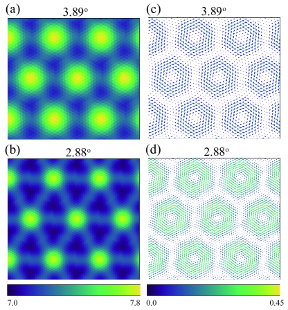
Figure 1: The relaxed structures of 3.89^∘ and 2.88^∘ twist MoTe₂ from DFT under dDsC vdWs correction. (a) and (b) are interlayer distances, determined by the distance between Mo atoms at the top and bottom layers. (c) and (d) are intralayer displacements, indicating the in-plane displacements after relaxations for Mo atoms at the top layer.

Large-scale DFT and lattice relaxation effect.

Making use of the initial moiré structure generated by deep potential molecular dynamics (DPMD) [37], we demonstrate that large-scale structural relaxations can be achieved at a significantly reduced computational cost. Remarkably, the relaxation of $\theta=2.88^{\circ}$ twisted structures comprising 2382 atoms was completed in just 5 hours with 17 DFT ionic steps using DPMD-generated structure in 4 NVIDIA H100 GPUs. The self-consistent caculation and band diagonalization of this 2382-atom system (IBAND=17160 and plane wave number 11469590) can be done within 80 minutes in 20 NVIDIA H100 GPUs, showcasing the massive speedup of the GPU platform for large-scale first principle simulation.

To demonstrate the relaxation effect in the $t$MoTe₂, we compare the relaxed moiré structures with twist angles $3.89^{\circ}$ and $2.88^{\circ}$. First, there is a big variation in the interlayer spacing (ILS) (Fig. 1), indicating a large structural transformation. For $t$MoTe₂ with a twist angle of $3.89^{\circ}$(Fig. 1(a)), the maximum ILS observed is 7.8 $\AA$. This occurs in the MM region, where the Te/Mo atoms of the top layer are aligned directly above those in the bottom layer, resulting in energy increase in this area due to the strong repulsion. The minimum ILS is 7.0 $\AA$, which is observed in the MX region where the Mo atoms of the top layer stack over the Te atoms of the bottom layer. Fig. 1(b) shows the ILS for $2.88^{\circ}$ $t$MoTe₂ exhibiting a clear domain wall connecting MM regions, which becomes more significant at lower twist angles as shown in supplemental materials [34].

Concerning the intralayer strain, both structures exhibit similar behaviors. As depicted in Fig. 1(c) and Fig. 1(d), the in-plane displacement pattern displays a helical chirality, with the amplitude intensifying as the twist angle diminishes. We observe a large displacement up to 0.5 $\AA$ for $\theta=2.88^{\circ}$, which generates a pseudo magnetic field up to $200$ $T$ [34].

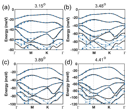
Figure 2: The comparative analysis of the band structures for twist angle (a) 3.15^∘ (b) 3.48^∘, (c) 3.89^∘, and (d) 4.41^∘, respectively. Blue points/lines illustrated the results from DFT calculations, while the black line represents the fitting results from continuum model.

Symmetry analysis of moiré band structures. The space group of the relaxed structures is $P321$ (No. 150), whose point group is generated by a two-fold rotational symmetry along $y$ axis ($C_{2y}$), and three-fold rotational symmetry along $z$ axis ($C_{3z}$). In the crystal momentum space, the $C_{2y}$ symmetry only protects two-fold degeneracies at the invariant lines or points within the Brillouin Zone, as defined by the relation $C_{2y}\mathbf{k}\rightarrow\mathbf{k}$. Within this invariant domain, the Hamiltonian commutes with the symmetry operation, allowing it to be block-diagonalized into two distinct sectors, each characterized by unique eigenvalues $\pm\pi$. Due to the constraints imposed by the symmetry, a band represented by $e^{i\pi}$ is inherently degenerate with another band represented by $e^{-i\pi}$, forming a doubly-degenerate band structure. Consequently, the only lines that encapsulate the $C_{2y}$ symmetries within the two-dimensional Brillouin zone are the $\Gamma K$ lines (satisfying $2\mathbf{k}_{1}+\mathbf{k}_{2}=0$). When considering the $C_{3z}$ rotational symmetry, the lines that meet the conditions $\mathbf{k}_{1}+2\mathbf{k}_{2}=0$ and $\mathbf{k}_{1}-\mathbf{k}_{2}=0$ also emerge as the symmetry-invariant lines. As a result, bands along the $\Gamma K$ and $MK$ lines are always doubly degenerate, while a clear splitting is observed along the $\Gamma M$ line as shown in Fig. 2.

In Fig. 3, we plot the angle dependent bandwidth and direct gap using two types of vdW corrections. At twist angle $\theta=3.89^{\circ}$, D2 type of vdW correction gives rise to a narrow bandwidth as 12 meV, which is close to previous calculation using local-basis SIESTA package [38] and D2 correction [21]. While under dDsC type of vdW correction, we obtain the bandwidth as 18 meV, and the overall trend of angle-dependent bandwidth follows a parabolic continuum behavior with single set of parameter as we will discuss later. At the smallest calculated twist angle $\theta=2.88^{\circ}$, the width of top moiré valence band reduced to 6 meV.

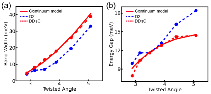
Figure 3: (a) Variation in bandwidth of the first and second moiré bands versus diverse twist angle. (b) Variation in direct band gap between the first two bands along the high symmetry lines in Fig. 2. Blue and red color denotes for the D2 (IVDW-10) and dDsC (IVDW-4) vdW correction, respectively.

Complete continuum model. We now introduce a more comprehensive continuum model to depict the moiré band structure. The key low-energy states originate from the hole bands in the $K$ and $K^{\prime}$ valleys of the two MoTe₂ layers. Considering that these valleys are connected through time reversal symmetry ($\mathcal{T}$), analyzing one valley is sufficient to infer the band structure. For twisted homobilayer TMD systems, which exhibit rotational ($C_{3z}$) and layer-exchange symmetry ($C_{2y}\mathcal{T}$), we derive the following form:

$$\hat{H}=\begin{bmatrix}-\frac{\bm{(\hat{k}-K_{t}+eA)^{2}}}{2m^{*}}+\Delta_{t}(\bm{r})&\Delta_{T}(\bm{r})\\ \Delta^{\dagger}_{T}(\bm{r})&-\frac{\bm{(\hat{k}-K_{b}-eA)^{2}}}{2m^{*}}+\Delta_{b}(\bm{r})\end{bmatrix}$$ (3)

with:

$$\Delta_{t}(\bm{r}) =2V_{1}\sum_{i=1,3,5}\cos(\bm{g^{1}_{i}\cdot r}+l\phi_{1})+2V_{2}\sum_{i=1,3,5}\cos(\bm{g^{2}_{i}\cdot r})$$ (4)

$$\Delta_{T} =w_{1}\sum_{i=1,2,3}e^{-i\bm{q^{1}_{i}\cdot r}}+w_{2}\sum_{i=1,2,3}e^{-i\bm{q^{2}_{i}\cdot r}}$$

$$A(\bm{r}) =A(\bm{a_{2}}\sin(\bm{G_{1}\cdot r})-\bm{a_{1}}\sin(\bm{G_{3}\cdot r})-\bm{a_{3}}\sin(\bm{G_{5}\cdot r}))$$

where $\bm{\hat{k}}$ is the momentum measured from the $\Gamma$ point of single layer MoTe₂, $\bm{K_{t}}(\bm{K_{b}})$ is high symmetry momentum $\bm{K}$ of the top(bottom) layer, $\Delta_{t}(\bm{r})(\Delta_{b}(\bm{r}))$ is the layer dependent moiré potential, $\Delta_{T}(\bm{r})$ is the interlayer tunneling, $\bm{G_{i}}$’s are moiré reciprocal vectors, $\bm{A}(\bm{r})$ is the strain induced gauge field which give a periodic pseudo magnetic field [27, 39]: $\bm{B(r)}=B\sum_{i=1,3,5}\cos(\bm{G_{i}\cdot r})$. $\bm{g_{i}^{1}}$ and $\bm{g_{i}^{2}}$ represent the momentum differences between the nearest and second-nearest plane wave bases within the same layer. Similarly, $\bm{q_{i}^{1}}$ and $\bm{q_{i}^{2}}$ denote the momentum differences between the nearest and second-nearest plane wave bases across different layers. $\bm{a_{1}},\bm{a_{2}},\bm{a_{3}}$ are the moire lattice vectors.(A comprehensive explanation of the moiré Brillouin zone and these vectors is provided in the Supplementary Materials S5).

To obtain accurate parameters in the continuum model, we perform large scale calculations with dDsC vdWs corrections (IVDW = 4), then fit the DFT moiré band structure at 3.15^∘ to obtain the following continuum parameter: $m^{*}=0.62m_{e},V_{1}=10.3$ meV,$V_{2}=2.9$ meV, $w_{1}=-7.8$ meV, $w_{2}=6.9$ meV, $\phi_{1}=-75^{\circ}$, $\Phi/\Phi_{0}=0.737$.($\Phi_{0}$ is the quantum flux, $\Phi$ represents the value of flux in moire unit cell). The continuum model parameters with D2 vdW corrections (IVDW = 10) are presented in the Supplementary Materials [34]. In our subsequent analysis of the continuum model, we will utilize the parameter from the IVDW = 4, as it provides the more reliable structure relaxation previously discussed. Employing these parameters, we are now equipped to solve the moiré band structures at various small twist angles.

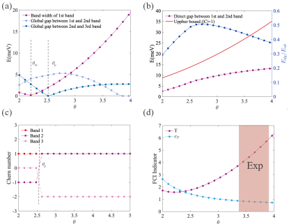
Figure 4: (a) The band width and global gap from the continuum model. There are gap closure happens between 2nd and 3rd band around $\theta_{p}\approx 2.5^{\circ}$. The bandwidth of the 1st band is denoted with the purple curve, which attains zero at the magic angle $\theta_{m}\approx 2.2^{\circ}$. (b) The direct gap between 1st and 2nd band and we note it always below the upper bound [40]. (c) The Chern number of the top three bands. There are a topological phase transition around 2.5^∘ owing to gap closure between 1st and 2nd band. (d) $T$ describes the violation of trace condition and $\sigma_{F}$ reflects the fluctuation of Berry curvature. We show them as a function of twist angles. The red region denotes the range of angles where FQAH effect are observed in transport experiments.

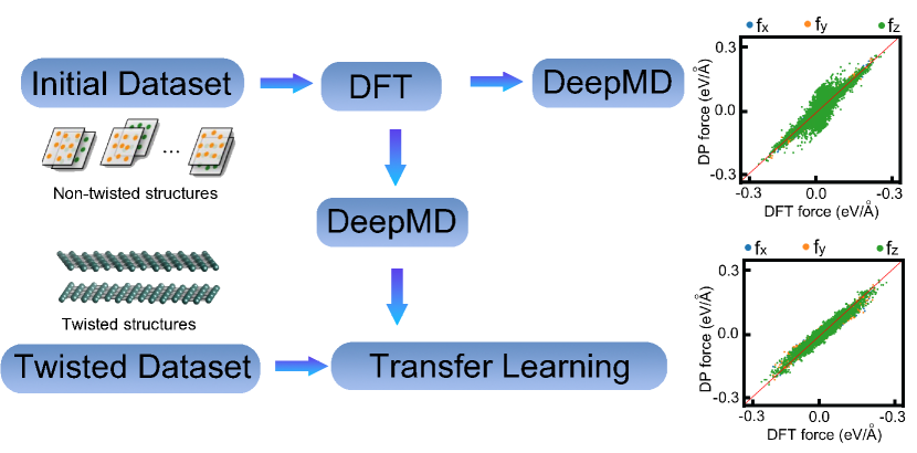
Figure 5: Scheme of Transfer Learning: A neural network trained solely on non-twisted structures struggles to accurately predict the forces in twisted structures. However, a neural network that undergoes transfer learning using a training set of twisted structures demonstrates a significantly improved ability to predict the forces accurately.

Next, we examine the topology of these moiré bands from 1.6^∘ to 5^∘. At twist angles below $2.5^{\circ}$, the Chern numbers for the top three bands, as calculated using the continuum model, are $1,-1,0$ as shown in Fig. 4(c). For greater twist angles, these Chern numbers change to $1,1,-2$. We emphasize that the arrangement of Chern numbers for $\theta>2.83^{\circ}$ is in agreement with experimental data. So far in all experiments where twist angle $\theta$ ranges between $3.5^{\circ}-3.9^{\circ}$, both [1, 2] the Hall conductance and the reflective magnetic circular dichroism increase once the doping exceeds $\nu=-1$. And a double quantum spin Hall effect has been observed at $\nu=-4$. These results suggest that the second band shares the same Chern number as the first band.

We additionally verify the trace condition for the uppermost moiré band. The band’s geometry is encapsulated in the quantum geometry tensor:

$$\eta^{uv}:=A_{BZ}\langle\partial^{u}u_{\bm{k}}\mid(1-|u_{\bm{k}}\rangle\langle u_{\bm{k}}|)\mid\partial^{v}u_{\bm{k}}\rangle$$ (5)

where $A_{BZ}$ is the area of the Brillouin zone. The symmetric and antisymmetric part of the quantum geometry tensor give the Berry curvature ($\Omega(\bm{k})=-2\mathrm{Im}(\eta^{xy})$) and quantum metric ($g^{uv}(\bm{k})=\mathrm{Re}(\eta^{uv})$). To quantify the geometric properties, one can calculate two figure of merits [41, 42, 43]:

$$\sigma_{F}: =\bigg{[}\frac{1}{A_{BZ}}\int d^{2}{\bm{k}}(\frac{\Omega(\bm{k})}{2\pi}-1)^{2}\bigg{]}^{\frac{1}{2}}$$ (6)

$$T: =\frac{1}{A_{BZ}}\int d^{2}{\bm{k}}\bigg{[}tr(g(\bm{k}))-\Omega(\bm{k})|\bigg{]},$$

where $\sigma_{F}$ describes the fluctuations of Berry curvature and the $T$ quantifies the violation of the trace condition. When both $\sigma_{F}$ and $T$ tend towards 0, it becomes possible to exactly map the Chern band to a Landau level problem allowing for intuitive understanding of the fractional state. We calculate the values of these parameters in relation to the twist angle, as depicted in Fig. 4(d).

Transfer learning structure relaxation. In order to resolve the problem of structural relaxation, we adopt the ab $initio$ deep potential (DP) molecular dynamics method, which combine the first-principles accuracy and empirical-potential efficiency for large-scale systems [37]. We begin with $3\times 3\times 1$ MM, MX, and XM configurations, along with 28 distinct intermediate transition states, all of which have been relaxed with a fixed volume. For each one of 31 configurations, We introduced random perturbations to generate 200 distinct structures. The random perturbations are applied to both the atomic coordinates, drawing values from a uniform distribution spanning [-0.01 $\AA$, 0.01 $\AA$], and the lattice constants, guided by a deformation matrix that is constructed from a distorted identity matrix spanning [-0.03, 0.03]. Besides, We conduct the 20 fs ab $initio$ molecular dynamics to gather VASP-calculated energy, force, and virial tensor, which constitute the entirety of initial training set.

Next, we train the initial DP model through the initial training set. We are using the two-body embedding smooth edition of the DeepPot-SE descriptor, which is constructed by both angular and radial of atomic configurations. The cut-off and smooth radius for neighbor searching are setting as 8.0 $\AA$ and 2.0 $\AA$, including a maximum number of 100 Mo and 100 Te atoms. Then, we construct a deep neural network that map the descriptors to atomic energy, through three embedding layers and three hidden layers of size (25, 50, 100) and (240, 240, 240), respectively. To measure the quality of deep neural network, we construct a loss function by a sum of different root means square errors (RMSE):

$$L\left(p_{\epsilon},p_{f},p_{\xi}\right)=\frac{p_{\epsilon}}{N}\Delta E^{2}+\frac{p_{f}}{3N}\sum_{i}\left|\Delta\bm{F}_{i}\right|^{2}+\frac{p_{\xi}}{9N}\|\Delta\Xi\|^{2},$$ (7)

where $\Delta E$, $\Delta\bm{F}_{i}$, and $\Delta\Xi$ refer to the RMSE of energy, force, and virial respectively. During the training process, the prefactor $p_{f}$ decrease from 1000 to 1, $p_{\epsilon}$ and $p_{\xi}$ increase from 0.02 to 1. To improve the efficiency of network training, we adopt an exponentially decaying learning rate to minimize the loss function. After 1 700 000 straining steps, the learning rate decrease from $1e^{-3}$ to a small value of $3.6e^{-8}$.

Then, the initially trained models are used to run molecular dynamics simulations for different pressures (-100 to 10000 bar) and temperatures (10 to 500K). A bunch of trajectories are generated in this process, and we could label them as the failure, candidate, or accurate configurations according to the model deviation:

$$\sigma_{f}^{\max}=\max\sqrt{\left\langle\left|\mathrm{F}_{i}-\left\langle\mathrm{F}_{i}\right\rangle\right|^{2}\right\rangle}.$$ (8)

During the process, 3 to 200 candidate configurations will be selected to perform the self-consistent DFT calculations, and the data will be collected for the training process of next-iteration.

Although the DP model show effective performance in the IVDW-10 correction, it does not yield successful results in the IVDW-4 correction, largely attributed to the complex dependencies on charge density. To address the issue, we augmente our training datasets with comprehensive data from large-angle twisted structures, encompassing forces, energies, and virial information, as illustrated in Fig. 5. Leveraging the principles of transfer learning, we strategically froze the parameters within the hidden and embedding layers while focusing on training the output layer. This approach significantly improves the performance of the pre-trained model, enabling it to adapt more effectively to the complexities of IVDW-4.

Atomic basis for small angle simulation. The OpenMX-calculated band structure agrees qualitatively with that from VASP calculation and further solidify the DFT results. Taking advantage of smaller size of Hamiltonian matrices under PAO basis, we use a denser $k$-point sampling along the $k$-path. We do statistics on the band width from results from both VASP and OpenMX, the results can be found in supplemental materials [34].

Conclusion. In this paper, we delve deeply into the lattice relaxation and single-particle of the twisted homobilayer MoTe₂ system. We present a comprehensive exploration of the moiré band structure under two type of vdW corrections, where we harness the power of large-scale density functional theory calculations together with transfer learning and GPU acceleration. Built on angle dependent moiré band structures, we construct the a more compete continuum model including higher harmonic potential and stain induced gauge field. Our calculations reveal that, at experimentally pertinent twist angles, the intralayer displacement induces a sizeable gauge field, and top two moiré bands consistently display nontrivial Chern numbers.

Impact on many body simulation. The continuum model parameters have strong impact on interaction-induced phases in $t$MoTe₂, as shown by previous numerical studies [22, 21, 44, 45, 23, 46, 24, 25, 47, 23, 48]. With continuum model fitted from D2 type of vdW correction [21], integer quantum anomalous Hall effect only appears at large dielectric constant $\epsilon>15$ [24, 25], and $\nu=-\frac{2}{3},-\frac{1}{3}$ are both found to be FCIs [21, 45]. With continuum model fitted from dDsC type of vdW correction [23, 22], the integer quantum anomalous Hall effect has been shown to occur at experimentally studied twist angles [24, 25], while $\nu=-\frac{2}{3}$ and $\nu=-\frac{1}{3}$ are FCI and charge density wave states, respectively [22, 25].

Note: Upon the completion of this work, a related work appeared [49], which has overlap with some of our calculations with IVDW=10.

Supplemental Materials

I.1 Density functional theory calculation and continuum model

We study TMD homobilayers with a small twist angle starting from AA stacking, where every metal (M) or chalcogen (X) atom on the top layer is aligned with the same type of atom on the bottom layer. Within a local region of a twisted bilayer, the atom configuration is identical to that of an untwisted bilayer, where one layer is laterally shifted relative to the other layer by a corresponding displacement vector ${\bm{d}}_{0}$. For this reason, the moiré band structures of twisted TMD bilayers can be constructed from a family of untwisted bilayers at various ${\bm{d}}_{0}$, all having $1\times 1$ unit cell. Our analysis thus starts from untwisted bilayers.

In particular, ${\bm{d}}_{0}=0,-\left({\bm{a}}_{1}+{\bm{a}}_{2}\right)/3,\left({\bm{a}}_{1}+{\bm{a}}_{2}\right)/3$, where ${\bm{a}}_{1,2}$ is the primitive lattice vector for untwisted bilayers, correspond to three high-symmetry stacking configurations of untwisted TMD bilayers, which we refer to as MM, XM, MX. In MM (MX) stacking, the M atom on the top layer is locally aligned with the M (X) atom on the bottom layer, likewise for XM. The bilayer structure in these stacking configurations is invariant under three-fold rotation around the $z$ axis. For the initial training datasets, we create untwisted TMD bilayers under a variety of interlayer displacement ${\bm{d}}_{0}$.

I.1.1 Details about plane-wave basis first principle calculations

The large-scale plane-wave basis first principle calculations are carried out with Perdew-Burke-Ernzerhof (PBE) functionals using the Vienna Ab initio simulation package (VASP). We choose the projector augmented wave potentials, incorporating 6 electrons for each of the Mo and Te atoms. During the structural relaxation, we set the plane wave cutoff energy and the energy convergence criterion to 250 eV and $1\times 10^{-6}$ eV, respectively. Larger energy cutoff of 350 eV and 500 eV has been tested for $\theta=3.89^{\circ}$, which leads to less than 1 meV change in the bandwidth of topmost valence band. The structure is fully relaxed when the convergence threshold for the maximum force experienced by each atom is less than 10 meV/$\AA$.

I.1.2 Details about local-basis first principles calculations

Apart from the calculation utilizing the plane-wave basis, our DFT study on twisted MoTe₂ has also been performed under the pseudo atomic orbital (PAO) basis. Using the relaxed atomic structures from VASP and DPMP, we use OpenMX package [50, 51] with PAOs chosen to be Mo7.0-s3p2d1 (7.0 means the cutoff radius is 7.0 Bohr, s3p2d1 means 3 sets of $s$-orbitals, 2 sets of $p$-orbitals and 1 set of $d$-orbitals, summed up as $3\times 1+2\times 3+1\times 5=14$ atomic orbitals for each Mo atom) and Te7.0-s3p2d2 to conduct the self-consisent calculation and obtain the band structure. The PBE exchange-correlation functional and the norm-conserving pseudopotential [52] are employed in the calculation with single $\Gamma$ $k$-sampling and convergence criterion no lower than 1.0$\times$10^-7 Hartree.

I.1.3 Assessment of different vdW corrections

Since the choice of vdW corrections largely influences relaxed interlayer distances in TMD materials, we accessed nine different vdW correction methods as implemented in VASP [53]. The projector augmented wave (PAW) method and the generalized gradient approximation (GGA) parameterized by Perdew-Burke-Ernzerhof [54, 55] are used for exchange-correlation potential. A self-consistent field method (tolerance $10^{-6}$ eV/atom) is employed in conjunction with a plane wave cutoff energy of 600 eV. Atomic structure optimization is performed until the Hellmann-Feynman forces on the ions are less than 0.0001 eV/Å. We used a $\Gamma$-centered $9\times 9\times 3$ $k$-point mesh to sample the BZ. All results are summarized in the SM [34]. For the bulk lattice constants, the vdW correction does not affect much the geometry relaxations. The bulk lattice constant $a$ and interlayer distance $d$ agree well with experiments and previous calculations. However, for the 2D moiré systems with large unit cells, the specific vdW corrected method heavily affected the numerical stability as well as the continuum model fitting. As shown in Fig. S1,  S2,  S3, and  S4, for each magic angle, the interlayer distances and intralayer displacements vary strongly with the employed vdW corrected methods.

Table S1: Predicted lattice parameters by different vdWs corrected methods for bulk-MoTe₂. $a$ is the lattice constant and $d$ is the vertical layer distance between the metal atoms at different layers. IVDW-I indicates the charge-density independent vdWs correction methods, whereas IVDW-II denotes the charge-density dependent vdW correction methods. Specifically, IVDW = 10 [31] denotes the DFT-D2 method of Grimme, IVDW = 11 [56] the DFT-D3 method of Grimme with zero-damping function, IVDW = 12 [57] the DFT-D3 method with Becke-Johnson damping function, and IVDW = 13 [58] the DFT-D4 method. IVDW = 3 [59] represents the DFT-ulg method, IVDW = 4 [32, 33] is the dDsC method, IVDW = 20 [60] is the Tkatchenko-Scheffler method, IVDW = 21 [61] is the Tkatchenko-Scheffler method with iterative Hirshfeld partitioning, and IVDW = 263 [62] is the many-body dispersion energy with fractionally ionic model for polarizability method.

	IVDW-I				IVDW-II
	10	11	12	13	3	4	20	21	263
$a$ (Å)	3.52	3.51	3.49	3.50	3.53	3.52	3.51	3.50	3.48
$d$ (Å)	6.99	7.00	6.83	6.85	7.11	7.02	6.95	6.94	6.90

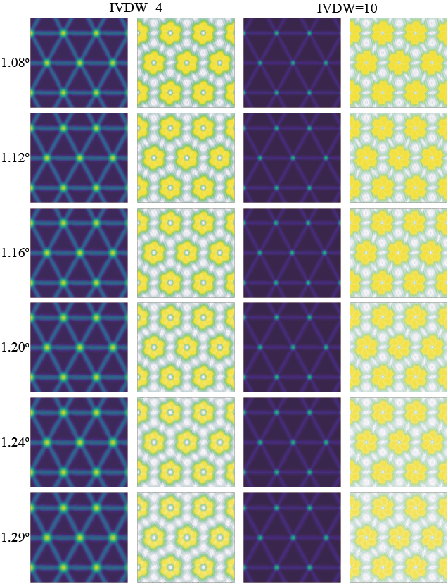
Figure S1: The interlayer distances and intralayer displacements of 1.08^∘, 1.12^∘, 1.16^∘, 1.20^∘, 1.24^∘, and 1.29^∘ $t$MoTe₂ by dDsC (IVDW = 4) and DFT-D2 (IVDW = 10) methods. The color bars employed in this section are identical to those presented in Fig. 1 of the main text.

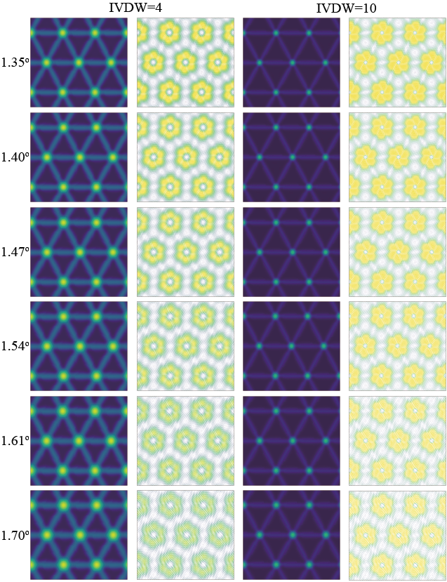
Figure S2: The interlayer distances and intralayer displacements of 1.35^∘, 1.40^∘, 1.47^∘, 1.54^∘, 1.61^∘, and 1.70^∘ $t$MoTe₂ by dDsC (IVDW = 4) and DFT-D2 (IVDW = 10) methods. The color bars employed in this section are identical to those presented in Fig. 1 of the main text.

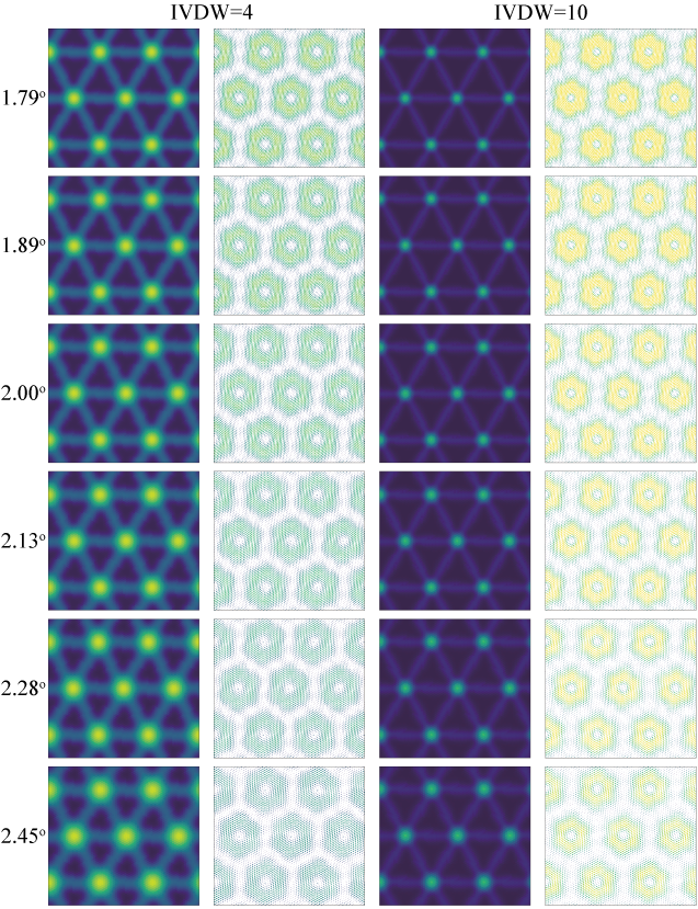
Figure S3: The interlayer distances and intralayer displacements of 1.79^∘, 1.89^∘, 2.00^∘, 2.13^∘, 2.28^∘, and 2.45^∘ $t$MoTe₂ by dDsC (IVDW = 4) and DFT-D2 (IVDW = 10) methods. The color bars employed in this section are identical to those presented in Fig. 1 of the main text.

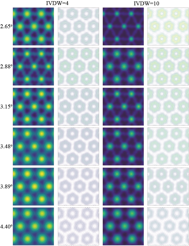
Figure S4: The interlayer distances and intralayer displacements of 2.65^∘, 2.88^∘, 3.15^∘, 3.48^∘, 3.89^∘, and 4.40^∘ $t$MoTe₂ by dDsC (IVDW = 4) and DFT-D2 (IVDW = 10) methods. The color bars employed in this section are identical to those presented in Fig. 1 of the main text.

I.2 The continuum model

I.2.1 The basis of continuum model

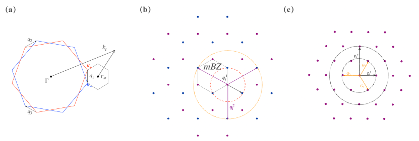
Figure S5: (a) The relation between the Brillouin zone (BZ) of single layer MoTe₂ and the moiré Brillouin zone (mBZ). The red (blue) hexagon is the BZ of top (bottom) layer MoTe₂ and the mBZ is shown with the small black hexagon. $\Gamma,K_{\pm}$ is the high symmetry points of single layer MoTe₂, $q_{1},q_{2},q_{3}$ are the momentum difference between two layer. $k_{t}$($k_{t}^{m}$) is the momentum of the plane wave basis which is measured realtive to the original point of BZ (mBZ). (b) The purple dot signifies the plane wave of the top layer ($Q_{+}$), while the blue dot represents that of the bottom layer($Q_{-}$). The 1st and 2nd harmonic term related interlayer coupling momentum $\bm{q^{1}_{i}}$ and $\bm{q^{2}_{i}}$ are illustrated here. (c) The 1st and 2nd harmonic term related intralayer coupling momentum $\bm{g^{1}_{i}}$ and $\bm{g^{2}_{i}}$ are illustrated here.

In this part, we would like to discuss the basis we use in the continuum model [63]. The low energy electron we include in the continuum model is the Bloch states of the single layer TMD near the $\bm{K_{\pm}}$, the interlayer and intra-layer coupling will couple them and give the final moire bands. We label the momentum of the Bloch states as:

$$\bm{k_{t}} =\bm{K_{+}-q_{3}+k_{t}^{m}}$$ (S1)

$$\bm{k_{b}} =\bm{K_{-}+q_{2}+k_{b}^{m}}$$

where $k_{t}$ is the Bloch states in the top layer and it is measured relative to the $\Gamma$ points of the single layer TMD and $k_{t}^{m}$ is measured relative to the $\Gamma_{M}$ of the moire Brillouin zone(mBZ), $\bm{q_{1}}$ is the momentum difference between the $K_{+}$ and $K_{-}$, $\bm{q_{2}}(\bm{q_{3}})$ is the $C_{3z}(C_{3z}^{-1})$ operate on the $\bm{q_{1}}$. We further restrict the momentum in the 1st mBZ and the formula will be:

$$\bm{k_{t}} =\bm{K_{+}-q_{3}+k_{t}^{m}+G_{m}}$$ (S2)

$$\bm{k_{b}} =\bm{K_{-}+q_{2}+k_{b}^{m}+G_{m}}$$

Note that $k_{t}^{m}$ and $k_{b}^{m}$ are in the 1st mBZ here. Then we use the relation between the $q_{i}$ and moire reciprocal vector, we finally arrive:

$$\bm{k_{t}} =\bm{K_{+}+k-Q_{+}}$$ (S3)

$$\bm{k_{b}} =\bm{K_{-}+k-Q_{-}}$$

where $\bm{Q_{\pm}=\pm q_{1}+G_{m}}$, they form a honeycomb lattice in K-space and all of symmetry can be kept with any finite cutoff, which gives a very convenient representation of the continuum model. The inter-layer interaction will transform into the coupling between the nearest neighbor momentum in the lattice and the intra-layer coupling will be the nearest intra-sub-lattice coupling. And then we introduce a continuous real space basis:

$$|l,\bm{r}\rangle=\frac{1}{\sqrt{\Omega_{tot}}}\sum_{\bm{k}}\sum_{\bm{Q}\in\bm{Q_{l}}}e^{-i(\bm{k-Q})\cdot\bm{r}}|\bm{k,Q}\rangle$$ (S4)

where $\Omega_{tot}$ is the total area of the system, $|\bm{k,Q}>$ is the Bloch state of single layer TMD. With the matrix of Hamiltonian under these basis, We next diagonalize it to get the eigenstate:

$$|\psi_{n\bm{k}}\rangle=\sum_{\bm{Q\in Q_{0}}}C_{n\bm{k}}(\bm{Q})|\bm{k,Q}\rangle$$ (S5)

Where the $C_{n\bm{k}}(\bm{Q})$ is the eigen-vector of the Hamiltonian. The real space distribution of the eigenstate is calculated with the real space continuous space basis:

$$\psi^{l}_{n\bm{k}}(\bm{r})=\langle l,\bm{r}|\psi_{n\bm{k}}\rangle =\sum_{\bm{Q\in Q_{0}}}C_{n\bm{k}}(\bm{Q})\langle l,\bm{r}|\bm{k,Q}\rangle$$ (S6)

$$=\frac{1}{\sqrt{\Omega_{tot}}}\sum_{\bm{Q\in Q_{l}}}C_{n\bm{k}}(\bm{Q})e^{i(\bm{k-Q})\cdot\bm{r}}$$

From this expression, we can see what we mean by using the plane wave as the basis.

I.2.2 The pseudo magnetic field under plane wave basis

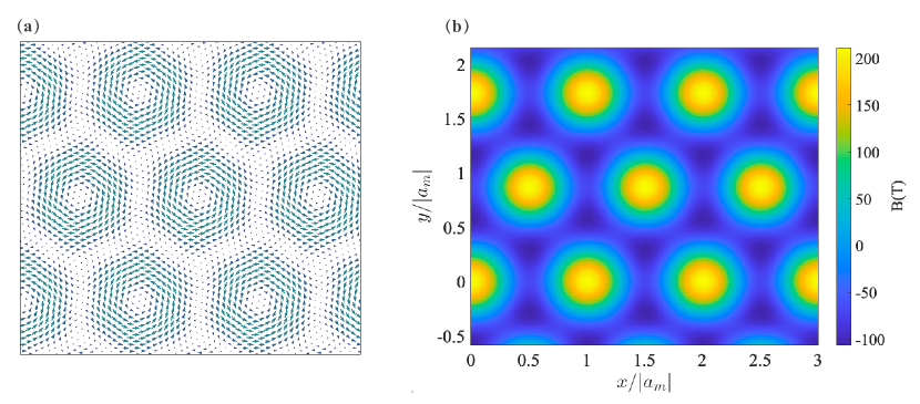
Figure S6: (a) The in-plane atom displacements with IVDW = 4 at $\theta=3.15^{\circ}$. (b) The distribution of pseudo magnetic field from our fitting results with $\frac{\Phi}{\Phi_{0}}=0.737$.

We consider a periodic pseudo-magnetic field (In the main text, we adopt $\phi=0$, but here we maintain it for general purposes.):

$$\bm{B}(\bm{r})=B\sum_{i=1,3,5}\cos(\bm{G_{i}\cdot r}+\phi)$$ (S7)

with the Coulomb gauge:$\nabla\cdot\bm{A}=0$, the vector potential reads($\bm{B}=\nabla\times\bm{A}$):

$$\bm{A}(\bm{r}) =A[a_{2}\sin(\bm{G_{1}\cdot r+\phi})-a_{1}\sin(\bm{G_{3}\cdot r+\phi})-a_{3}\sin(\bm{G_{5}\cdot r}+\phi)]$$ (S8)

$$=AL_{m}f(\bm{r})$$

where:

$$\bm{a_{1}} =[\frac{\sqrt{3}}{2},-\frac{1}{2}]L_{m}$$ (S9)

$$\bm{a_{2}} =[\frac{\sqrt{3}}{2},+\frac{1}{2}]L_{m}$$

$$\bm{a_{3}} =\bm{a_{2}-a_{1}}$$

$$A =\frac{\sqrt{3}B}{4\pi}$$

$$\bm{G_{i}} =\frac{4\pi}{\sqrt{3}L_{m}}[\cos(i-2)\frac{\pi}{3},\sin(i-2)\frac{\pi}{3}]$$

The Hamiltonian of the single layer reads:

$$H(\bm{r}) =-\frac{[\bm{p+eA(r)}]^{2}}{2m^{*}}+V(\bm{r})$$ (S10)

$$=-\frac{\bm{p}^{2}}{2m}-\frac{e}{m^{*}}\bm{A(r)\cdot p}-\frac{e^{2}}{2m^{*}}\bm{A^{2}(r)}+V(\bm{r})$$

The first order term:

$$H_{A} =-\frac{e}{m^{*}}\frac{\sqrt{3}B}{4\pi}L_{m}f(\bm{r})\cdot\hbar\bm{k}$$ (S11)

$$=-\frac{\hbar^{2}}{m^{*}L_{m}}\frac{\Phi}{\Phi_{0}}f(\bm{r})\cdot\bm{k}$$

The second order term:

$$H_{A^{2}} =-\frac{e^{2}}{2m^{*}}\bm{A^{2}(r)}$$ (S12)

$$=-\frac{e^{2}}{2m^{*}}A^{2}L_{m}^{2}f^{2}(\bm{r})$$

$$=-\frac{\hbar^{2}}{2m^{*}L_{m}^{2}}\frac{\Phi^{2}}{\Phi_{0}^{2}}f^{2}(\bm{r})$$

where $\Phi$ is the flux in the moire unit cell, $\Phi_{0}=\frac{h}{e}$ represent the quantum flux. In our calculation, we choose: $\frac{\hbar^{2}}{m_{0}}=7.62eV\cdot\AA^{2}$. With the plane wave basis:

$$|\bm{K_{\pm}+k-Q_{\pm}}\rangle$$ (S13)

The first order reads:

$$H_{A}= \frac{\sqrt{3}\gamma_{1}B_{r}}{4i}(e^{i\phi}\delta_{\bm{Q,Q^{\prime}+G_{4}}}-e^{-i\phi}\delta_{\bm{Q,Q^{\prime}+G_{1}}}+e^{-i\phi}\delta_{\bm{Q,Q^{\prime}+G_{3}}}-e^{i\phi}\delta_{\bm{Q,Q^{\prime}+G_{6}}})(\bm{k-Q^{\prime}})_{x}...$$ (S14)

$$+ \frac{\gamma_{1}B_{r}}{4i}(e^{i\phi}\delta_{\bm{Q,Q^{\prime}+G_{4}}}-e^{-i\phi}\delta_{\bm{Q,Q^{\prime}+G_{1}}}+e^{i\phi}\delta_{\bm{Q,Q^{\prime}+G_{6}}}-e^{-i\phi}\delta_{\bm{Q,Q^{\prime}+G_{3}}}$$

$$+2e^{-i\phi}\delta_{\bm{Q,Q^{\prime}+G_{5}}}-2e^{i\phi}\delta_{\bm{Q,Q^{\prime}+G_{2}}})(\bm{k-Q^{\prime}})_{y}$$

The second order term:

$$H^{part1}_{A^{2}}=\gamma_{2}B_{r}^{2}\bigg{(}\frac{3}{2}\delta_{\bm{Q,Q^{\prime}}}-\sum_{i=1,3,5}\bigg{(}\frac{e^{-2i\phi}}{4}\delta_{\bm{Q,Q^{\prime}+2G_{i}}}+\frac{e^{2i\phi}}{4}\delta_{\bm{Q,Q^{\prime}-2G_{i}}}\bigg{)}\bigg{)}$$ (S15)

$$H^{part2}_{A^{2}} =\gamma_{2}B_{r}^{2}\bigg{(}\sin(\bm{G_{3}\cdot r+\phi)}\sin(\bm{G_{5}\cdot r+\phi})-\sin(\bm{G_{1}\cdot r+\phi)}\sin(\bm{G_{5}\cdot r+\phi})-\sin(\bm{G_{1}\cdot r+\phi)}\sin(\bm{G_{3}\cdot r+\phi})\bigg{)}$$ (S16)

$$=\frac{\gamma_{2}B_{r}^{2}}{4}\bigg{[}\bigg{(}\delta_{\bm{Q,Q^{\prime}-G_{3}+G_{5}}}+\delta_{\bm{Q,Q^{\prime}+G_{5}-G_{3}}}-e^{i2\phi}\delta_{\bm{Q,Q^{\prime}-G_{3}-G_{5}}}-e^{-i2\phi}\delta_{\bm{Q,Q^{\prime}+G_{3}+G_{5}}}\bigg{)}$$

$$-\bigg{(}\delta_{\bm{Q,Q^{\prime}-G_{1}+G_{5}}}+\delta_{\bm{Q,Q^{\prime}+G_{5}-G_{1}}}-e^{i2\phi}\delta_{\bm{Q,Q^{\prime}-G_{1}-G_{5}}}-e^{-i2\phi}\delta_{\bm{Q,Q^{\prime}+G_{1}+G_{5}}}\bigg{)}$$

$$-\bigg{(}\delta_{\bm{Q,Q^{\prime}-G_{1}+G_{3}}}+\delta_{\bm{Q,Q^{\prime}+G_{3}-G_{1}}}-e^{i2\phi}\delta_{\bm{Q,Q^{\prime}-G_{1}-G_{3}}}-e^{-i2\phi}\delta_{\bm{Q,Q^{\prime}+G_{1}+G_{3}}}\bigg{)}$$

I.3 Fitting of continuum model at various twist angles

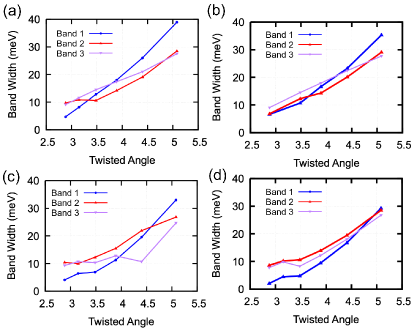
Figure S7: (a, c) Bandwidth variation of the first three bands in DFT calculations under dDsC (IVDW-4) and D2 (IVDW-10) corrections, respectively. (b, d) Bandwidth variation of the first three bands in Open-MX calculations under dDsC (IVDW-4) and D2 (IVDW-10) corrections, respectively.

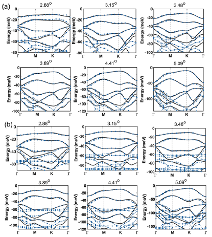
Figure S8: The comparative analysis of the band structures at twist angles of 2.88^∘, 3.15^∘, 3.48^∘, 3.89^∘, 4.41^∘, and 5.09^∘, under (a) dDsC (IVDW-4) and (b) D2 (IVDW-10) corrections. Blue points and lines represent results from DFT calculations, while black lines illustrate the fitting from the continuum model, with each twist angle employing a distinct set of parameters.

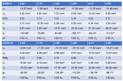
Figure S9: The fitting parameters at twist angles of 2.88^∘, 3.15^∘, 3.48^∘, 3.89^∘, 4.41^∘, and 5.09^∘ adjusted by specific twist angles, under dDsC (IVDW-4) and D2 (IVDW-10) corrections. We note the fitting parameters for dDsC (IVDW-4) is smooth and less angle dependent.

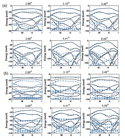
Figure S10: The comparative analysis of the band structures at twist angles of 2.88^∘, 3.15^∘, 3.48^∘, 3.89^∘, 4.41^∘, and 5.09^∘, under (a) dDsC (IVDW-4) and (b) D2 (IVDW-10) corrections. Black lines represent results from DFT calculations, while blue points and lines illustrate the fitting from the continuum model, with each vdWs correction sharing the same set of parameters.

We refine the model parameters by fitting the eigenvalues of the spin-up Hamiltonian, with the corresponding values derived from fully relativistic band structure calculations using VASP. For achieving heightened precision in the continuum model parameters with D2 vdW corrections (IVDW = 10), we fit the DFT moiré band structure at a twist angle of 3.89^∘, leading to the determination of the following continuum parameters: $m^{*}=0.62m_{e}$, $V_{1}=7.88$ meV, $V_{2}=22.72$ meV, $w_{1}=-11.60$ meV, $w_{2}=12.02$ meV, $\phi_{1}=-88^{\circ}$, and $\Phi/\Phi_{0}$ = 0.02. Employing these parameters, we are now equipped to solve the moiré band structures at various small twist angles. Furthermore, we have also employed different parameters to fit various twisted angles and vdW corrections, as depicted in the Fig. S10.

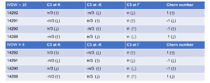
Figure S11: The $C_{3z}$ symmetry eigenvalues of the high symmetry momentum points, computed from large-scale DFT wavefunctions at a twist angle of 2.88^∘, under dDsC (IVDW-4) and D2 (IVDW-10) corrections.

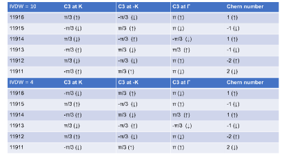
Figure S12: The $C_{3z}$ symmetry eigenvalues of the high symmetry momentum points, computed from large-scale DFT wavefunctions at a twist angle of 3.15^∘, under dDsC (IVDW-4) and D2 (IVDW-10) corrections.

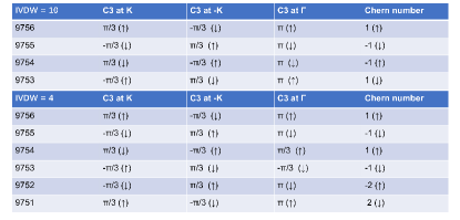
Figure S13: The $C_{3z}$ symmetry eigenvalues of the high symmetry momentum points, computed from large-scale DFT wavefunctions at a twist angle of 3.48^∘, under dDsC (IVDW-4) and D2 (IVDW-10) corrections.

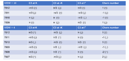
Figure S14: The $C_{3z}$ symmetry eigenvalues of the high symmetry momentum points, computed from large-scale DFT wavefunctions at a twist angle of 3.89^∘, under dDsC (IVDW-4) and D2 (IVDW-10) corrections.

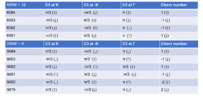
Figure S15: The $C_{3z}$ symmetry eigenvalues of the high symmetry momentum points, computed from large-scale DFT wavefunctions at a twist angle of 4.41^∘, under dDsC (IVDW-4) and D2 (IVDW-10) corrections.

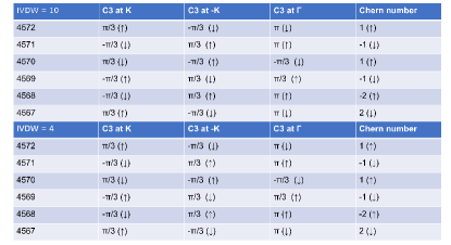
Figure S16: The $C_{3z}$ symmetry eigenvalues of the high symmetry momentum points, computed from large-scale DFT wavefunctions at a twist angle of 5.09^∘, under dDsC (IVDW-4) and D2 (IVDW-10) corrections.

References

- Cai et al. [2023] J. Cai, E. Anderson, C. Wang, X. Zhang, X. Liu, W. Holtzmann, Y. Zhang, F. Fan, T. Taniguchi, K. Watanabe, et al., Nature , 1 (2023).
- Zeng et al. [2023] Y. Zeng, Z. Xia, K. Kang, J. Zhu, P. Knüppel, C. Vaswani, K. Watanabe, T. Taniguchi, K. F. Mak, and J. Shan, Nature , 1 (2023).
- Park et al. [2023] H. Park, J. Cai, E. Anderson, Y. Zhang, J. Zhu, X. Liu, C. Wang, W. Holtzmann, C. Hu, Z. Liu, et al., Nature , 1 (2023).
- Xu et al. [2023a] F. Xu, Z. Sun, T. Jia, C. Liu, C. Xu, C. Li, Y. Gu, K. Watanabe, T. Taniguchi, B. Tong, et al., Physical Review X 13, 031037 (2023a).
- Devakul et al. [2021] T. Devakul, V. Crépel, Y. Zhang, and L. Fu, Nature communications 12, 1 (2021).
- Li et al. [2021] H. Li, U. Kumar, K. Sun, and S.-Z. Lin, Phys. Rev. Res. 3, L032070 (2021).
- Crépel and Fu [2022] V. Crépel and L. Fu, arXiv:2207.08895 (2022).
- Wu et al. [2019] F. Wu, T. Lovorn, E. Tutuc, I. Martin, and A. MacDonald, Phys. Rev. Lett. 122, 086402 (2019).
- Tang et al. [2011] E. Tang, J.-W. Mei, and X.-G. Wen, Phys. Rev. Lett. 106, 236802 (2011).
- Sheng et al. [2011] D. Sheng, Z.-C. Gu, K. Sun, and L. Sheng, Nat. Commun. 2, 389 (2011).
- Regnault and Bernevig [2011] N. Regnault and B. A. Bernevig, Physical Review X 1, 021014 (2011).
- Sun et al. [2011] K. Sun, Z. Gu, H. Katsura, and S. D. Sarma, Physical review letters 106, 236803 (2011).
- Neupert et al. [2011] T. Neupert, L. Santos, C. Chamon, and C. Mudry, Physical review letters 106, 236804 (2011).
- Xiao et al. [2011] D. Xiao, W. Zhu, Y. Ran, N. Nagaosa, and S. Okamoto, Nat. Commun. 2, 596 (2011).
- Venderbos et al. [2012] J. W. Venderbos, S. Kourtis, J. van den Brink, and M. Daghofer, Physical Review Letters 108, 126405 (2012).
- Bergholtz and Liu [2013] E. J. Bergholtz and Z. Liu, Int. J. Mod. Phys. B 27, 1330017 (2013).
- Neupert et al. [2015] T. Neupert, C. Chamon, T. Iadecola, L. H. Santos, and C. Mudry, Phys. Scr. 2015, 014005 (2015).
- Liu and Bergholtz [2023] Z. Liu and E. J. Bergholtz, in Reference Module in Materials Science and Materials Engineering (Elsevier, 2023) p. B9780323908009001360.
- Parameswaran et al. [2013] S. A. Parameswaran, R. Roy, and S. L. Sondhi, C. R. Phys. 14, 816 (2013).
- Nayak et al. [2008] C. Nayak, S. H. Simon, A. Stern, M. Freedman, and S. Das Sarma, Rev. Mod. Phys. 80, 1083 (2008).
- Wang et al. [2023a] C. Wang, X.-W. Zhang, X. Liu, Y. He, X. Xu, Y. Ran, T. Cao, and D. Xiao, arXiv preprint arXiv:2304.11864 (2023a).
- Reddy et al. [2023] A. P. Reddy, F. F. Alsallom, Y. Zhang, T. Devakul, and L. Fu, arXiv preprint arXiv:2304.12261 (2023).
- Xu et al. [2023b] C. Xu, J. Li, Y. Xu, Z. Bi, and Y. Zhang, arXiv preprint arXiv:2308.09697 (2023b).
- Yu et al. [2023] J. Yu, J. Herzog-Arbeitman, M. Wang, O. Vafek, B. A. Bernevig, and N. Regnault, arXiv preprint arXiv:2309.14429 (2023).
- Abouelkomsan et al. [2023] A. Abouelkomsan, A. P. Reddy, L. Fu, and E. J. Bergholtz, arXiv preprint arXiv:2309.16548 (2023).
- Naik and Jain [2018] M. H. Naik and M. Jain, Physical review letters 121, 266401 (2018).
- Yu et al. [2020] H. Yu, M. Chen, and W. Yao, Natl. Sci. Rev. 7, 12 (2020).
- Xian et al. [2020] L. Xian, M. Claassen, D. Kiese, M. M. Scherer, S. Trebst, D. M. Kennes, and A. Rubio, arXiv preprint arXiv:2004.02964 (2020).
- Zhang et al. [2021] Y. Zhang, T. Liu, and L. Fu, Physical Review B 103, 155142 (2021).
- Angeli and MacDonald [2021] M. Angeli and A. H. MacDonald, Proceedings of the National Academy of Sciences 118, e2021826118 (2021).
- Grimme [2006] S. Grimme, Journal of Computational Chemistry 27, 1787 (2006).
- Steinmann and Corminboeuf [2011a] S. N. Steinmann and C. Corminboeuf, The Journal of chemical physics 134 (2011a).
- Steinmann and Corminboeuf [2011b] S. N. Steinmann and C. Corminboeuf, Journal of chemical theory and computation 7, 3567 (2011b).
- [34] See Supplemental Material for the full details on the derivations.
- Wilson and Yoffe [1969] J. A. Wilson and A. Yoffe, Advances in Physics 18, 193 (1969).
- Reshak and Auluck [2005] A. H. Reshak and S. Auluck, Phys. Rev. B 71, 155114 (2005).
- Zhang et al. [2018] L. Zhang, J. Han, H. Wang, R. Car, and E. Weinan, Physical review letters 120, 143001 (2018).
- García et al. [2020] A. García, N. Papior, A. Akhtar, E. Artacho, V. Blum, E. Bosoni, P. Brandimarte, M. Brandbyge, J. I. Cerdá, F. Corsetti, et al., The Journal of chemical physics 152 (2020).
- Xie et al. [2022] Y.-M. Xie, C.-P. Zhang, J.-X. Hu, K. F. Mak, and K. T. Law, Physical Review Letters 128, 026402 (2022).
- Onishi and Fu [2023] Y. Onishi and L. Fu, Fundamental bound on topological gap (2023), arXiv:2306.00078 [cond-mat.mes-hall] .
- Roy [2014] R. Roy, Physical Review B 90, 165139 (2014).
- Parameswaran et al. [2012] S. Parameswaran, R. Roy, and S. L. Sondhi, Physical Review B 85, 241308 (2012).
- Claassen et al. [2015] M. Claassen, C. H. Lee, R. Thomale, X.-L. Qi, and T. P. Devereaux, Physical review letters 114, 236802 (2015).
- Goldman et al. [2023] H. Goldman, A. P. Reddy, N. Paul, and L. Fu, arXiv preprint arXiv:2306.02513 (2023).
- Dong et al. [2023] J. Dong, J. Wang, P. J. Ledwith, A. Vishwanath, and D. E. Parker, arXiv preprint arXiv:2306.01719 (2023).
- Reddy and Fu [2023] A. P. Reddy and L. Fu, arXiv preprint arXiv:2308.10406 (2023).
- Qiu et al. [2023] W.-X. Qiu, B. Li, X.-J. Luo, and F. Wu, arXiv preprint arXiv:2305.01006 (2023).
- Wang et al. [2023b] T. Wang, T. Devakul, M. P. Zaletel, and L. Fu, arXiv preprint arXiv:2306.02501 (2023b).
- Jia et al. [2023] Y. Jia, J. Yu, J. Liu, J. Herzog-Arbeitman, Z. Qi, N. Regnault, H. Weng, B. A. Bernevig, and Q. Wu, Moiré fractional chern insulators i: First-principles calculations and continuum models of twisted bilayer mote2 (2023), arXiv:2311.04958 [cond-mat.mes-hall] .
- Ozaki and Kino [2004] T. Ozaki and H. Kino, Physical Review B 69, 195113 (2004).
- Ozaki [2003] T. Ozaki, Physical Review B 67, 155108 (2003).
- Morrison et al. [1993] I. Morrison, D. M. Bylander, and L. Kleinman, Physical Review B 47, 6728 (1993).
- Kresse and Hafner [1993] G. Kresse and J. Hafner, Phys. Rev. B 47, 558 (1993).
- Blöchl [1994] P. E. Blöchl, Phys. Rev. B 50, 17953 (1994).
- Perdew et al. [1996] J. P. Perdew, K. Burke, and M. Ernzerhof, Phys. Rev. Lett. 77, 3865 (1996).
- Grimme et al. [2010] S. Grimme, J. Antony, S. Ehrlich, and H. Krieg, J. Chem. Phys. 132 (2010).
- Grimme et al. [2011] S. Grimme, S. Ehrlich, and L. Goerigk, J. Comput. Chem.” 32, 1456 (2011).
- Caldeweyher et al. [2019] E. Caldeweyher, S. Ehlert, A. Hansen, H. Neugebauer, S. Spicher, C. Bannwarth, and S. Grimme, J. Chem. Phys. 150 (2019).
- Kim et al. [2012] H. Kim, J.-M. Choi, and W. A. Goddard III, J. Phys. Chem. Lett. 3, 360 (2012).
- Tkatchenko and Scheffler [2009] A. Tkatchenko and M. Scheffler, Phys. Rev. Lett. 102, 073005 (2009).
- Bučko et al. [2014] T. Bučko, S. Lebègue, J. G. Ángyán, and J. Hafner, J. Chem. Phys. 141 (2014).
- Gould and Bucko [2016] T. Gould and T. Bucko, J. Chem. Theory Comput. 12, 3603 (2016).
- Bernevig et al. [2021] B. A. Bernevig, Z.-D. Song, N. Regnault, and B. Lian, PHYSICAL REVIEW B 103, 10.1103/PhysRevB.103.205411 (2021).