PICS in Pics: Physics Informed Contour Selection for Rapid Image Segmentation

Abstract

Effective training of deep image segmentation models is challenging due to the need for abundant, high-quality annotations. Generating annotations is laborious and time-consuming for human experts, especially in medical image segmentation. To facilitate image annotation, we introduce Physics Informed Contour Selection (PICS) - an interpretable, physics-informed algorithm for rapid image segmentation without relying on labeled data. PICS draws inspiration from physics-informed neural networks (PINNs) and an active contour model called snake. It is fast and computationally lightweight because it employs cubic splines instead of a deep neural network as a basis function. Its training parameters are physically interpretable because they directly represent control knots of the segmentation curve. Traditional snakes involve minimization of the edge-based loss functionals by deriving the Euler-Lagrange equation followed by its numerical solution. However, PICS directly minimizes the loss functional, bypassing the Euler Lagrange equations. It is the first snake variant to minimize a region-based loss function instead of traditional edge-based loss functions. PICS uniquely models the three-dimensional (3D) segmentation process with an unsteady partial differential equation (PDE), which allows accelerated segmentation via transfer learning. To demonstrate its effectiveness, we apply PICS for 3D segmentation of the left ventricle on a publicly available cardiac dataset. While doing so, we also introduce a new convexity-preserving loss term that encodes the shape information of the left ventricle to enhance PICS’s segmentation quality. Overall, PICS presents several novelties in network architecture, transfer learning, and physics-inspired losses for image segmentation, thereby showing promising outcomes and potential for further refinement.

Keywords Physics Informed Neural Network  $\cdot$ Active Contour Model  $\cdot$ Image Segmentation  $\cdot$ Chan-Vese Functional  $\cdot$ Transfer Learning

1 Introduction

Deep learning-based computer vision models have achieved remarkable success in various medical imaging tasks. However, their reliance on large amounts of labeled data can limit their utility in situations where data is scarce or unavailable. This limitation has spurred significant recent advancements in the field of physics-informed computer vision (PICV), as discussed in Banerjee et al. [banerjee2023physicsinformed].

The term "physics-informed" in PICV is largely attributed to the development of the Physics Informed Neural Network (PINN) by Raissi et al. [RAISSI2019]. PINNs have shown promise in addressing forward and inverse problems related to partial differential equations (PDEs) in fields like fluid mechanics [raissi2018hidden, dwivedi2020physics], material modeling [Liu2019], heat transfer [cai2021, dwivedi2021distributed], and more [Karniadakis2021].

Inspired by the philosophy behind PINNs, PICV integrates physical principles into machine learning frameworks for computer vision. This approach results in faster, more interpretable, and data-efficient computer vision models. In context of medical imaging, some recent examples are as follows. Lopez et al.[ARRATIALOPEZ2023102925] recently introduced WarpPINN, a physics-informed neural network designed for image registration to assess local metrics of heart deformation. They incorporated the near-incompressibility of cardiac tissue by penalizing the Jacobian of the deformation field. Similarly, Vries et al.[DEVRIES2023102971] developed a PINN-based model to estimate CT perfusion parameters from noisy data related to acute ischemic stroke. Herten et al.[VANHERTEN2022102399] utilized PINNs for tracer-kinetic modeling and parameter inference using myocardial perfusion medical resonance imaging (MRI) data. Buoso and collaborators proposed a parametric PINN for simulating personalized left-ventricular biomechanics, offering the potential to significantly expedite training data synthesis [BUOSO2021102066]. Additionally, Burwinkel et al.[BURWINKEL2022102314] introduced OpticNet, an innovative optical refraction network that utilizes an unsupervised, domain-specific loss function to explicitly incorporate ophthalmological information into the network.

Our primary focus in this study is image segmentation, which involves identifying and delineating distinct regions or objects within an image. The approaches to image segmentation can be broadly categorized into two extremes: deep learning-based models that rely on substantial labeled training data and traditional models that do not require training data but face challenges related to some theoretical and numerical aspects.

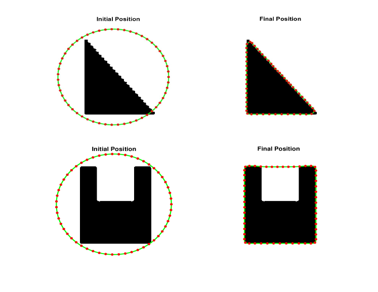
Figure 1: Image segmentation with a naive image gradient-based snake. In the cavity case, please note that it gets stuck to a local minima.

Among all active contour models, snake[Kass1988] is the most intuitive image segmentation model. It is based on the concept of a deformable curve or surface that can be iteratively adjusted to fit the edges or boundaries of an object in an image. The contour is driven by internal energy, which represents the smoothness of the curve, and external energy, which is derived from image features such as intensity or texture. By minimizing the total energy, the contour can accurately delineate the object boundaries, thus facilitating object recognition and tracking. For example, refer to Fig.1. At the start, the snake (or deformable contour) has maximum energy, and following the minimization process, it converges to the object’s boundary. In mathematical terms, snakes detect object boundaries by minimizing edge-based energy functionals, achieved through the solution of the Euler-Lagrange equations.

Despite being very intuitive, snakes suffer from the following numerical issues [sapiro2006geometric]:

1. They are sensitive to initialization.

2. They don’t work well with noisy data, which can be a significant issue in real-world scenarios where data may be incomplete or corrupted.

3. Use of snake require sophisticated numerical methods [Prince1997, Xie2008, Wang2009, COHEN1991211] to solve Euler-Lagrange equations.

4. Hyperparameter tuning can be challenging, as selecting optimal parameters for the model can be time-consuming and require significant expertise.

5. Snakes can’t handle topology changes, which occur when objects in the image intersect or touch.

6. It is difficult to incorporate prior domain knowledge in the form of energy functionals, which can limit the model’s ability to leverage existing domain knowledge.

In this work, we propose PICS (Physics Informed Contour Selection) that integrates snakes and PINNs in a manner that capitalizes on the strengths of both approaches while mitigating their weaknesses. To accomplish this, we modified the PINN approach by introducing the following novelties:

• Custom design the PINN hypothesis (network architecture) to effectively capture object boundaries. PINNs use a deep neural network (see eq.6) with a large number of parameters to approximate the solution, whereas PICS employs cubic splines (see eq.23) that can efficiently approximate any closed contour with only a few control knots. The use of a simplified architecture leads to significant speed ups as compared to traditional PINNs[dwivedi2020physics, dwivedi2021distributed, biharmonic2020, normal2021].

• Assign control knots as a design variable. In most deep neural networks, the weights are typically initialized randomly and do not have any physical significance. However, PICS is formulated in such a way that trainable weights are represented by the control knots of cubic splines. It gives it a clear physical meaning to weights that simplifies scaling and normalization steps. Similarly, the loss gradient in PICS can be physically interpreted as the force on the control knots pushing them towards the direction of gradient descent.

• Minimize region-based loss instead of gradient-based loss functionals. PICS enhances the stability of snakes towards noisy data by optimizing region-based energy functionals [mumford1989optimal, chan2001active] instead of relying solely on edge-based energy functionals [Kass1988, Prince1997, Xie2008, COHEN1991211]. This approach has never been attempted in traditional numerical or deep learning frameworks because there is no explicit differentiable function for the derivative of the region-based loss with respect to snake control knots. We are the first to address this issue by implicitly calculating the loss derivatives through finite difference methods.

• Incorporate prior shape information via regularization terms. Like the parent PINN, PICS can easily accommodate any prior information about the shape of the object via shape-based regularization terms.

• Exploit transfer learning for 3D segmentation. Given multiple 2D slices of a 3D object, PICS exploits transfer learning to reuse the optimized weights (spline control knots) from the previous slice as the initial condition for segmenting the current slice. This modality allows the snake to quickly converge to the optimal segmentation for each slice, reducing the number of iterations required for convergence and the overall computational cost.

To demonstrate the effectiveness of PICS, we take an example from the field of medical image segmentation. Medical image segmentation is a critical step in disease diagnosis, treatment planning, and medical research[bai2020population, mei2020artificial, kickingereder2019automated, wang2019benchmark]. This process involves locating the regions of interest from medical images, such as magnetic resonance imaging (MRI) or computerized tomography (CT) scans, which can be used to identify and diagnose abnormalities, tumors, and other medical conditions. In recent years, medical image segmentation has been revolutionized by the rapid development of deep learning algorithms for computer vision[badrinarayanan2017segnet, long2015fully, ronneberger2015u]. These algorithms have shown impressive results[litjens2017survey, shen2017deep, hesamian2019deep, li2018h, dolz2018hyperdense, haberl2018cdeep3m] in accurately segmenting medical images, thus improving the accuracy and efficiency of medical diagnosis and treatment. However, their success heavily depends on the quality and quantity of the training data[rahimi2021addressing, lecun2015deep, webb2018deep]. The problem is that acquiring high-quality medical images with labels (also called masks) requires expert interpretation [https://doi.org/10.48550/arxiv.1711.08037], and it is a labor-intensive and time-consuming process[segars2013population, oktay2020evaluation]. Furthermore, the automatic tools are not trusted[duran2021afraid] within the medical community. Therefore, PICS can fill a crucial research gap by serving as an intuitive tool for medical practitioners to generate rapid annotations, addressing the limitations associated with acquiring labeled medical images and improving the efficiency of the segmentation process.

The organization of this paper is as follows. We start with a brief review of snakes and PINN. Next, we list the objectives of the paper. In the Methods section, we describe the mathematical formulation of PICS. Then, we discuss the results in Results section. Finally, the conclusions of the paper are given at the end.

2 Brief Review of Snake and PINN

2.1 Brief Review of Snake Model

Consider Fig.1 in which the snake (or deformable contour) has maximum energy at the start, and following the minimization process, it converges to the object’s boundary. Mathematically, if the total energy of the snake is given by

$$J=\frac{\alpha}{2}\intop_{0}^{1}\psi_{s}^{2}ds+\frac{\beta}{2}\intop_{0}^{1}\psi_{ss}^{2}ds+J_{ext}$$ (1)

where $(s,t)$ denote space and time parameters respectively, $\psi$ denotes the parametric spline used for segmentation contour, $(\alpha,\beta)$ are the coefficients, the sum of first two terms denotes the internal energy ($J_{int}$) of the snake and $J_{ext}$ denotes external energy.

Then, the motion of the snake is governed by the following PDE:

$$\frac{\partial\vv{\psi}}{\partial t}=\alpha\frac{\partial^{2}\vv{\psi}}{\partial s^{2}}+\beta\frac{\partial^{4}\vv{\psi}}{\partial s^{4}}-\nabla J_{ext}$$ (2)

The internal energy controls the smoothness of snake and it is independent of the data. However, $J_{ext}$ is an image dependent, edge-based functional. For example, if $I$ is the image, then a simple gradient-based $J_{ext}$ could be $J_{ext}=-\int_{0}^{1}|\nabla I|^{2}ds$. For such functionals, a differentiable function for the gradient of $J_{ext}$ with respect to control knots cannot be found. However, if $J_{ext}$ is a region-based functional (for example, refer equation 16), then the expression for $\nabla J_{ext}$ with respect to control knots cannot be directly found. If the object has weak gradients and the image is noisy, the denoising also removes the object boundary. In such cases, region-based loss functions are beneficial, but the traditional snake framework is not suitable for their implementation.

2.2 Brief Review of PINNs

Figure 2: Distribution of collocation (red triangles) and boundary points (blue rectangles) in the computational domain.

In a typical PINN, the solution of PDE is approximated by a deep neural network. The training data, which consists of collocation and boundary points (see Fig.2), are randomly distributed in the computational domain. For example, consider the following one-dimensional (1D) unsteady PDE.

$$\frac{\partial}{\partial t}u(x,t)+\mathcal{\mathcal{\mathscr{N}}}u(x,t)=R(x,t),(x,t)\in\Omega$$ (3)

$$u(x,t)=B(x,t),(x,t)\in\partial\Omega,$$ (4)

$$u(x,0)=F(x),x\in(x_{L},x_{R}),$$ (5)

where $\mathcal{\mathscr{N}}$ is a nonlinear differential operator and $\partial\Omega$ is the boundary of the computational domain $\Omega$. We approximate $u$ with a $n$-layered deep neural network $\psi$ such that

$$\psi=\psi(z;W_{1},W_{2}...W_{n},b_{1},b_{2},...b_{n})=W_{n}(...(\phi(W_{2}(\phi(W_{1}z+b_{1}))+b_{2}))...)+b_{n}$$ (6)

where $z=[x,t]^{T}$denote sampling points, $(W_{i},b_{i})$ denote model parameters and $\phi$ denotes nonlinearity. For PINNs, $z$ are randomly selected, but after selection, they remain fixed. If we denote the errors in approximating the PDE, BCs, and IC by $\vv{\xi}_{f}$, $\vv{\xi}_{bc}$ and $\vv{\xi}_{ic}$ respectively. Then, the expressions for these errors are as follows:

$$\vv{\xi}_{f}=\frac{\partial\vv{\psi}}{\partial t}+\mathcal{\mathcal{\mathscr{N}}}\vv{\psi}-\vv{R},\;on\;(\vv{x}_{f},\vv{y}_{f})$$ (7)

$$\vv{\xi}_{bc}=\vv{\psi}-\vv{B},\>(\vv{x}_{bc},\vv{t}_{bc})_{side\>faces}$$ (8)

$$\vv{\xi}_{ic}=\vv{\psi}(.,0)-\vv{F},\>(\vv{x}_{bc},\vv{t}_{bc})_{bottom\>face}$$ (9)

For shallow networks, $\frac{\partial\vv{\psi}}{\partial t}$ and $\mathcal{\mathcal{\mathscr{N}}}\vv{\psi}$ can be determined using hand calculations. However, for deep networks, we have to use finite difference methods or automatic differentiation [baydin2018automatic]. The latter is preferred for its computational efficiency. We can recast the PDE, BC, IC system to an optimization problem by minimizing an appropriate loss function. The loss function $J$ to be minimized for a PINN is given by

$$J=\frac{\vv{\xi}_{f}^{T}\vv{\xi}_{f}}{2N_{f}}+\frac{\vv{\xi}_{bc}^{T}\vv{\xi}_{bc}}{2N_{bc}}+\frac{\vv{\xi}_{ic}^{T}\vv{\xi}_{ic}}{2N_{ic}},$$ (10)

where $N_{f}$, $N_{bc}$, and $N_{ic}$ refer to the number of collocation points, boundary condition points in left and right faces, and initial condition points at the bottom face, respectively. We can see that we have chosen a least square loss function. Now, any gradient based optimization routine may be used to minimize $J$.

3 Objectives

The objective of the paper is to demonstrate the effectiveness of the PICS in performing image segmentation in both 2D and 3D settings, with and without prior knowledge of the object’s shape. Specifically speaking,

1. Given a 2D image, perform segmentation with and without prior shape information.

2. Given a 3D image, perform segmentation with and without prior shape information.

3. Discuss hyperparameter tuning for simple and complex images.

Furthermore, the paper aims to evaluate the performance of the method against labeled data to assess its accuracy and reliability.

4 Methods

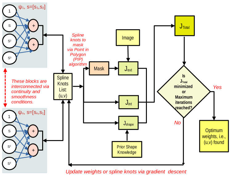
Figure 3: Overview of PICS algorithm.

Figure 3 shows the overall flowchart of PICS. In this section, we will describe its individual components, i.e., (a) PICS hypothesis, (b) the Chan-Vese loss function, (c) optimization,(d) the prior shape-based loss term, and (e) the operation performance index (OPI)–a metric to monitor the optimization performance of PICS.

4.1 PICS Hypothesis

We approximate the solution in PICS, i.e., object boundary with a parametric spline. The expression of parametric spline $\vv{\psi}$ is given by

(23)