Personalized Federated Learning via ADMM with Moreau Envelope

Abstract

Personalized federated learning (PFL) is an approach proposed to address the issue of poor convergence on heterogeneous data. However, most existing PFL frameworks require strong assumptions for convergence. In this paper, we propose an alternating direction method of multipliers (ADMM) for training PFL models with Moreau envelope (FLAME), which achieves a sublinear convergence rate, relying on the relatively weak assumption of gradient Lipschitz continuity. Moreover, due to the gradient-free nature of ADMM, FLAME alleviates the need for hyperparameter tuning, particularly in avoiding the adjustment of the learning rate when training the global model. In addition, we propose a biased client selection strategy to expedite the convergence of training of PFL models. Our theoretical analysis establishes the global convergence under both unbiased and biased client selection strategies. Our experiments validate that FLAME, when trained on heterogeneous data, outperforms state-of-the-art methods in terms of model performance. Regarding communication efficiency, it exhibits an average speedup of 3.75$\times$ compared to the baselines. Furthermore, experimental results validate that the biased client selection strategy speeds up the convergence of both personalized and global models.

1 Introduction

Federated learning (FL) plays a crucial role in the field of artificial intelligence [32], particularly in critical applications such as next-word prediction [14], smart healthcare [35, 3], and its recent integration into emerging large language models (LLMs) [46, 20, 6]. This innovative technique enables the collaborative training of models across devices while preserving privacy and security [19, 25].

Despite the advantages of FL in preserving privacy, it still encounters challenges with respect to the statistical heterogeneity of data, affecting its performance and convergence [27, 28, 16]. The statistical heterogeneity of data in FL primarily manifests in the non-independent and non-identically distributed (non-i.i.d.) data across different clients [59]. When training FL models on non-i.i.d. data, the generalization error significantly increases due to data heterogeneity, which can cause the model to converge in different directions [9, 44]. Personalization has garnered significant attention in addressing data heterogeneity in the context of FL [45]. For example, within the setting of next-word prediction, when different users input “I like to eat $\cdots$”, the predictions provided by the input method editor should be personalized to cater to the specific preferences of different users [37, 14].

Personalized federated learning (PFL) can be employed to train personalized models for individual users, catering to their distinct preferences. Numerous PFL frameworks have been proposed for training models on heterogeneous data [45]. One of the most well-known approaches formulates the objective function of PFL as a bi-level optimization problem [58], utilizing the Moreau envelope [34], and employs first-order gradient methods (such as SGD) to optimize personalized and global models alternately [44, 26]. However, existing PFL frameworks rely on strong assumptions for convergence, including gradient Lipschitz continuity, bounded variance, and bounded diversity [44]. Furthermore, these frameworks establish convergence solely in the context of random (also referred to as unbiased) client selection, yet they fail to address the issue of enhancing PFL efficiency by determining which clients should participate in the training process. Moreover, SGD typically demands the manual fine-tuning of the learning rate, a highly sensitive hyperparameter [13]. An excessively large learning rate can trigger model instability or even divergence, whereas an overly small learning rate leads to sluggish convergence and an elevated risk of becoming trapped in local minima. As a result, discovering the right learning rate often entails iterative experimentation and adjustment. Nevertheless, in scenarios such as training LLMs within PFL, the computational resources and time needed for a single model training iteration are substantial. Engaging in empirical parameter tuning can substantially increase both the training time and resource consumption.

To address these issues, we propose FLAME, a PFL framework with Moreau envelope based on ADMM for training models. Our contributions are summarized as follows:

• We transform the bi-level optimization problem of PFL into a multi-block optimization problem and solve it using ADMM, which eliminates the need to adjust the learning rate during the training of the global model.

• We propose a biased client selection strategy, primarily achieved by involving clients with larger update messages in the training process. Furthermore, we propose estimating the model’s update messages using local gradients and selecting clients with larger local gradients before each communication, which speeds up the convergence.

• We establish sublinear convergence rates for FLAME for both unbiased and biased client selection strategies under the weak assumption of gradient Lipschitz continuity. Additionally, we theoretically demonstrate that the biased client strategy, which prioritizes clients with larger gradients for updates, can expedite convergence.

• We validated the algorithm’s effectiveness on four datasets. FLAME exhibits superior convergence performance on heterogeneous data compared to state-of-the-art methods, achieving a 2.7$\times$ speedup in communication rounds. Moreover, our proposed biased client selection strategy can speed up the convergence of both personalized and global models.

The remaining content is structured as follows: Section 2 presents the related work, Section 3 introduces the preliminaries used in our study, Section 4 outlines our proposed method, FLAME, Section 5 validates our algorithm through experiments, and Section 6 concludes our paper.

2 Related Work

Due to our consideration of addressing the impact of data heterogeneity on the training model in federated learning, we first review several specific patterns of data heterogeneity. Subsequently, we review recent research on the adoption of the primal-dual framework within FL and how PFL methods can mitigate the impact of data heterogeneity on training FL models. Finally, we review recent research on client selection to explain why these methods are not applicable to our approach.

2.1 Data Heterogeneity

Ye et al. [55] categorized the statistical heterogeneity of data into four distinct skew patterns: label skew, feature skew, quality skew, and quantity skew. Label skew refers to the dissimilarity in label distributions among the participating clients [19, 56]. Feature skew denotes a situation in which the feature distributions among participating clients diverge [24, 30]. Quality skew illustrates the inconsistency in data collection quality across different clients [54]. Quantity skew denotes an imbalance in the amount of local data across clients [40]. Fig. 1 shows examples of the four skew patterns. These skew patterns result in non-i.i.d. data collected from various clients, leading to local models converging in different directions [55], thereby resulting in the trained global model not being the optimum. This can result in the performance of FL models potentially being inferior even to that of locally trained models [27, 63, 18, 33, 51].

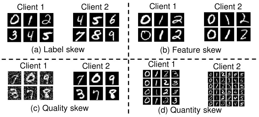
Figure 1: Four skew patterns: (a) the labels vary among different clients; (b) the features of the data differ among different clients, manifested as variations in the stroke thickness and slant angle; (c) the data quality varies, notably due to the presence of noise; (d) the quantity of data differs among clients.

2.2 Primal-dual Scheme for Federated Learning

In recent years, primal-dual schemes have gained widespread utilization in the context of FL [31, 41, 42, 12, 61, 62, 64]. Smith et al. [31, 42, 17] introduced a distributed machine learning framework which utilizes a stochastic dual coordinate ascent (SDCA) [39] method to solve the dual problem. Building upon this framework, Smith et al. [41] proposed a multi-task FL framework to train models for multiple related tasks simultaneously. However, since these frameworks require solving dual problems, they are only applicable to convex problems. Zhang et al. [57] introduced a primal-dual FL framework designed to handle non-convex objective functions. However, this method suffers restrictive assumptions for convergence. Zhou and Li [61] proposed the FedADMM, establishing convergence under mild conditions. Gong et al. [12] proposed that within FedADMM, the dual variables can effectively mitigate the impact of data heterogeneity on the training model. Based on FedADMM, Zhou and Li [62] proposed a method that differs from FedADMM by performing a single step of gradient descent on the unselected clients, thereby enhancing communication efficiency.

2.3 Personalized Federated Learning

Personalization was proposed to address the impact of data heterogeneity on training FL models. Tan et al. [45] categorized the strategies of PFL into two classes: global model personalization [60, 27, 8, 49] and learning personalized models [10, 9, 44]. Zhao et al. [60] proposed an approach involving the initial training of a warm-up model utilizing shared data stored on the server. However, this approach requires data sharing among clients, involving privacy risks. Li et al. [27] incorporated a proximal term into the sub-problem of each client, taking into account the differences between the global FL model and local models, with the aim of fine-tuning the influence of local updates. However, these methods exhibit limited improvements in the performance of FL models on heterogeneous data. Finn et al. [10] considered a model-agnostic meta-learning (MAML) algorithm that is designed to be compatible with different learning problems, enabling the training of a model across various tasks. Inspired by the principles of MAML, Fallah et al. [9] introduced Per-FedAvg, which builds an initial meta-model that can be efficiently updated with a single additional gradient descent step. Inspired by Per-FedAvg, Dinh et al. [44] proposed pFedMe, currently a state-of-the-art approach, implementing multiple gradient descent steps within the meta-model update process to enhance the solution precision.

2.4 Client Selection

In the conventional setting of FL, the unbiased client selection strategy is commonly employed, randomly choosing several clients to participate in each training round [29]. However, this approach of randomly sampling clients during each training round leads to several drawbacks, including reduced model accuracy, slower convergence rate, and compromised fairness [11, 53]. To address this issue, some studies have proposed selecting clients with superior communication and computational capabilities to engage in each round of training [36, 52, 21, 2, 23, 43]. However, these approaches limit the effective participation of clients with weaker hardware capabilities, consequently resulting in the failure to fully exploit the local updates from diverse clients. Horváth and Richtárik [15] first analyzed the biased client selection in FL by focusing on the perspective of selecting clients with higher local losses. Building on the idea of prioritizing clients with the highest loss, Cho et al. [7] proposed Power-of-Choice, a client selection strategy that expedites convergence, along with theoretical convergence analysis. In contrast to selecting clients with higher local losses, Wu and Wang [48] proposed selecting clients by identifying the optimal subset of local updates through gradient-based exclusion of adverse updates. However, these methods suffer a common issue, i.e., the inability to ascertain whether they can speed up the convergence in the context of PFL, and lack a theoretical guarantee for convergence.

Remarks. 1) The convergence of existing PFL frameworks still relies on strong assumptions (gradient Lipschitz continuity, bounded variance, and bounded diversity); 2) Existing PFL frameworks rely on first-order gradient methods for training personalized and global models, leading to challenges in hyperparameter tuning; 3) Existing client selection strategies intensify the impact of data heterogeneity on the training model. Furthermore, there is currently no client selection strategy specifically designed for PFL.

3 Preliminaries

In this section, we provide an explanation of the notations used in this paper, offer a detailed description of the definition of FL, introduce the concept of ADMM, and present an overview of the Moreau envelope.

3.1 Notations

We use different text formatting styles to represent different mathematical concepts: plain letters for scalars, bold letters for vectors, and capitalized letters for matrices. For instance, $m$ represents a scalar, $\boldsymbol{w}$ represents a vector, and $W$ denotes a matrix. Without loss of generality, all training models in this paper are represented using vectors. We use $[m]$ to represent the set $\{1,2,...,m\}$. The symbol $\mathbb{E}$ denotes the expectation of a random variable, and we use “$:=$” to indicate a definition, while $\mathbb{R}^{n}$ represents the $n$-dimensional Euclidean space. We represent the inner product of vectors, such as $\langle\boldsymbol{a},\boldsymbol{b}\rangle$, as the sum of the products of their corresponding elements. We use $||\cdot||$ to denote the Euclidean norm of a vector, and the Spectral norm of a matrix.

3.2 Federated Learning

Consider an FL scenario with $m$ clients, where each client $i$ possesses a local dataset $X_{i}$ comprising $n_{i}$ data samples with data distribution $\mathcal{D}_{i}$. These clients are interconnected through a central server and aim to collectively train a model $\boldsymbol{w}$ that minimizes the empirical risk [32]:

$$\min_{\boldsymbol{w}}\left\{\sum_{i=1}^{m}\alpha_{i}f_{i}(\boldsymbol{w}):=\sum_{i=1}^{m}\alpha_{i}\mathbb{E}_{\boldsymbol{x}\sim\mathcal{D}_{i}}[\ell_{i}(\boldsymbol{w};\boldsymbol{x})]\right\},$$ (1)

where $\alpha_{i}$ is a weight parameter, $f_{i}(w):=\mathbb{E}_{\boldsymbol{x}\sim\mathcal{D}_{i}}[\ell_{i}(\boldsymbol{w};\boldsymbol{x})]$ denotes the expected loss over the data distribution of client $i$, $\boldsymbol{x}$ is a random data sample drawn from $\mathcal{D}_{i}$, and $\ell_{i}(\boldsymbol{w};\boldsymbol{x})$ denotes the loss function for sample $\boldsymbol{x}$ with respect to model $\boldsymbol{w}$. Typically, the value of $\alpha_{i}$ is set to $1/m$ or $n_{i}/n$, where $n=\sum_{i=1}^{m}n_{i}$ is the total number of data points.

3.3 Alternating Direction Method of Multipliers

ADMM is an optimization method that belongs to the class of augmented Lagrangian methods and is particularly well-suited for solving the following general problem [4]:

$$\min_{\boldsymbol{w}\in\mathbb{R}^{r},\boldsymbol{v}\in\mathbb{R}^{q}}f(\boldsymbol{w})+g(\boldsymbol{v}),\quad\text{s.t. }A\boldsymbol{w}+B\boldsymbol{v}-\boldsymbol{b}=\boldsymbol{0},$$

where $A\in\mathbb{R}^{p\times r}$, $B\in\mathbb{R}^{p\times q}$, and $\boldsymbol{b}\in\mathbb{R}^{p}$. We directly give its augmented Lagrangian function as follows,

$$\begin{split}\mathcal{L}(\boldsymbol{w},\boldsymbol{v},\boldsymbol{\pi})&:=f(\boldsymbol{w})+g(\boldsymbol{v})\\ &+\langle\boldsymbol{\pi},A\boldsymbol{w}+B\boldsymbol{v}-\boldsymbol{b}\rangle+\frac{\rho}{2}||A\boldsymbol{w}+B\boldsymbol{v}-\boldsymbol{b}||^{2},\end{split}$$

where $\boldsymbol{\pi}\in\mathbb{R}^{p}$ is the dual variable, and $\rho>0$ is the penalty parameter. After initializing the variables with $(\boldsymbol{w}^{0},\boldsymbol{v}^{0},\boldsymbol{\pi}^{0})$, ADMM iteratively performs the following steps:

$$\begin{split}\boldsymbol{w}^{t+1}&=\operatorname{argmin}_{\mathbf{w}\in\mathbb{R}^{r}}\mathcal{L}(\boldsymbol{w},\boldsymbol{v}^{t},\boldsymbol{\pi}^{t}),\\ \boldsymbol{v}^{t+1}&=\operatorname{argmin}_{\boldsymbol{v}\in\mathbb{R}^{q}}\mathcal{L}(\boldsymbol{w}^{t+1},\boldsymbol{v},\boldsymbol{\pi}^{t}),\\ \boldsymbol{\pi}^{t+1}&=\boldsymbol{\pi}^{t}+\rho(A\boldsymbol{w}^{t+1}+B\boldsymbol{v}^{t+1}-\boldsymbol{b}).\end{split}$$

ADMM exhibits distributed and parallel computing capabilities, effectively addresses equality-constrained problems, and provides global convergence guarantees [47]. It finds widespread applications in distributed computing, machine learning, and related fields, making it particularly well-suited for tackling large-scale optimization problems.

3.4 Moreau Envelope

The Moreau envelope is an essential concept in the fields of mathematics and optimization [34]. It finds widespread application in convex analysis, nonsmooth optimization, and numerical optimization. Here, we present the definition of the Moreau envelope.

Definition 1 (Moreau envelope [38]).

Consider a function $f:\mathbb{R}^{p}\rightarrow\mathbb{R}$, its Moreau envelope is defined as:

$$F(\boldsymbol{w}):=\min_{\boldsymbol{\theta}\in\mathbb{R}^{p}}f(\boldsymbol{\theta})+\frac{\lambda}{2}||\boldsymbol{w}-\boldsymbol{\theta}||^{2},$$ (2)

where $\lambda$ is a hyperparameter. Its associated proximal operator is defined as:

$$\hat{\boldsymbol{\theta}}(\boldsymbol{w}):=\text{prox}_{f/\lambda}(w)=\operatorname*{argmin}_{\boldsymbol{\theta}\in\mathbb{R}^{p}}\left\{f(\boldsymbol{\theta})+\frac{\lambda}{2}||\boldsymbol{\theta}-\boldsymbol{w}||\right\}.$$ (3)

The Moreau envelope provides a smooth approximation of the original function $f$. This approximation is helpful when dealing with optimization algorithms that require smooth functions. As $\lambda$ becomes smaller, the Moreau envelope approaches the original function, making it useful for approximating and optimizing non-smooth functions. Next, we describe a useful property of Moreau envelope [38].

Proposition 1.

If $f$ is a proper, lower semicontinuous, and weakly convex (or nonconvex with $L$-Lipschitz $\nabla f$), then $F$ is $L_{F}$-smooth with $L_{F}=\lambda$ (with the condition that $\lambda>2L$ for nonconvex $L$-smooth $f$), and the gradient of $F$ is defined as:

$$\nabla F(\boldsymbol{w})=\lambda(\boldsymbol{w}-\hat{\boldsymbol{\theta}}(\boldsymbol{w})).$$ (4)

4 Proposed FLAME

In this section, we initially present the formulation of the optimization problem for PFL based on ADMM. Subsequently, we provide an algorithmic description of FLAME along with a specific example. Following this, we introduce unbiased and biased client selection strategies and establish the theoretical convergence analysis under both strategies.

Input: $T:$ the total communication rounds, $\rho$: the penalty parameter, $\lambda$: the hyperparameter, $m$: the number of clients, $X_{i},i\in[m]$: the local dataset, $\eta$: the learning rate, $H$: the number of inner iterations.

1 Initialize: $\boldsymbol{\theta}_{i}^{0},\boldsymbol{w}_{i}^{0},\boldsymbol{\pi}_{i}^{0},\boldsymbol{z}_{i}^{0}=\boldsymbol{w}_{i}^{0}+\frac{1}{\rho}\boldsymbol{\pi}_{i}^{0}$, $i\in[m]$, $biased\_flag$.

2for $t=0,1,\dots,T-1$ do

       /* On the server side. */

       Select $s$ clients by calling ClientSelection($biased\_flag$);

        // Client selection

3      

      Call each client, uploading $\{\boldsymbol{z}^{t}_{1},\dots,\boldsymbol{z}^{t}_{m}\}$ to the server;

        // Upload the update messages

4      

      Update $\boldsymbol{w}^{t}=\frac{1}{m}\sum_{i=1}^{m}\boldsymbol{z}_{i}^{t}$;

        // Update the global model

5      

      Broadcast $\boldsymbol{w}^{t}$ to the selected clients;

        // Broadcast the global model

6      

      /* On the client side. */

7      

8      for each client $i\in\mathcal{S}^{t}$ do

             Creat Batches $\mathcal{B}$;

              // Gradient descent for solving personalized model

9            

10            for $h=0,1,\dots,H-1$ do

11                   for batch $\xi\in\mathcal{B}$ do

12                         Compute the gradient $f_{i}(\boldsymbol{\theta}_{i}^{t,h},\xi)$;

13                        

14                        $\boldsymbol{\theta}_{i}^{t,h+1}=\boldsymbol{\theta}_{i}^{t,h}-\eta(\nabla f_{i}(\boldsymbol{\theta}_{i}^{t,h},\mathcal{B})+\lambda(\boldsymbol{\theta}_{i}^{t,h}-\boldsymbol{w}_{i}^{t}))$;

15                        

            $\boldsymbol{\theta}_{i}^{t+1}=\boldsymbol{\theta}_{i}^{t,H-1}$;

              // Update the personalized model

16            

            $\boldsymbol{w}_{i}^{t+1}=\frac{1}{\lambda\alpha_{i}+\rho}(\lambda\alpha_{i}\boldsymbol{\theta}_{i}^{t+1}+\rho\boldsymbol{w}^{t}-\boldsymbol{\pi}_{i}^{t})$;

              // Update the local model

17            

            $\boldsymbol{\pi}_{i}^{t+1}=\boldsymbol{\pi}_{i}^{t}+\rho(\boldsymbol{w}_{i}^{t+1}-\boldsymbol{w}^{t})$;

              // Update the dual variable

18            

            $\boldsymbol{z}_{i}^{t+1}=\boldsymbol{w}_{i}^{t+1}+\frac{1}{\rho}\boldsymbol{\pi}_{i}^{t+1}$;

              // Compute the update message

19            

20      for each client $i\notin\mathcal{S}^{t}$ do

             $(\boldsymbol{\theta}_{i}^{t+1},\boldsymbol{w}_{i}^{t+1},\boldsymbol{\pi}_{i}^{t+1},\boldsymbol{z}_{i}^{t+1})=(\boldsymbol{\theta}_{i}^{t},\boldsymbol{w}_{i}^{t},\boldsymbol{\pi}_{i}^{t},\boldsymbol{z}_{i}^{t})$;

              // Local parameters remain unchanged

21            

22

23 

/* Two client selection strategies. */

24 Function ClientSelection($biased\_flag$):

25       if $biased\_flag=True$ then

             /* Biased client selection strategy. */

             Randomly select $c$ clients $\mathcal{C}^{t}\subset[m]$;

              // Select a candidate client set

26            

27            for each client $i\in\mathcal{C}^{t}$ do

28                  

29                  Randomly sample a mini-batch $\xi$;

30                  

31                  Compute $g_{i}=\nabla f_{i}(\boldsymbol{\theta}_{i}^{t,h},\mathcal{\xi})+\lambda(\boldsymbol{\theta}_{i}^{t,h}-\boldsymbol{w}_{i}^{t})$;

32                  

            Get $\mathcal{S}^{t}=\{s\text{ clients with largest }||g_{i}||\}$;

              // Select $s$ clients with the largest gradient

33            

34      else if $biased\_flag=False$ then

             /* Unbiased client selection strategy. */

35            

36            Randomly select $s$ clients $\mathcal{S}^{t}\subset[m]$;

37            

38      

39return $\mathcal{S}^{t}$;

Algorithm 1 FLAME

4.1 Problem Formulation

To construct the objective function for PFL, we employ the approach outlined in [44], where the Moreau envelope of $f_{i}$ is substituted for $f_{i}$ in optimization Problem (1). The specific formulation of the problem is presented as follows:

$$\begin{split}&\min_{\boldsymbol{w}}\!\sum_{i=1}^{m}\alpha_{i}F_{i}(\boldsymbol{w}),\\ \text{where }F_{i}(\boldsymbol{w}):=&\min_{\boldsymbol{\theta}_{i}}f_{i}(\boldsymbol{\theta}_{i})+\frac{\lambda}{2}||\boldsymbol{\theta}_{i}-\boldsymbol{w}||^{2},\quad i\in[m].\end{split}$$ (5)

Note that $F_{i}$ is the Moreau envelope of $f_{i}$, and $\boldsymbol{\theta}_{i}$ is the personalized model of client $i$. The hyperparameter $\lambda$ controls the influence of the global model $\boldsymbol{w}$ on the personalized model $\boldsymbol{\theta}_{i}$. A higher value of $\lambda$ provides an advantage to clients with unreliable data by harnessing extensive data aggregation, whereas a lower $\lambda$ places greater emphasis on personalization for clients with a substantial amount of useful data. Note that $\lambda\in(0,\infty)$ to prevent extreme cases where $\lambda=0$ (no FL) or $\lambda=\infty$ (no PFL). The overall concept is to enable clients to develop their personalized models in different directions while remaining close to the global model $\boldsymbol{w}$ contributed by every client. Note that Problem (5) is a bi-level optimization problem. The conventional approach to solving bi-level problems typically involves initially using a first-order gradient method to solve $\boldsymbol{\theta}_{i}$ in the lower-level problem, obtaining an approximate solution. This approximate solution is then incorporated into the upper-level problem, followed by another round of the first-order gradient method to solve $\boldsymbol{w}$ in the upper-level problem. Iterating through this process multiple times yields the final solutions. Even though the first-order gradient method is simple, it is cumbersome to fine-tune parameters, such as the learning rate. To address this issue, we propose a relaxed form of Problem (5):

$$\min_{\boldsymbol{w},\boldsymbol{\theta}_{i}}\sum_{i=1}^{m}\alpha_{i}\left(f_{i}(\boldsymbol{\theta}_{i})+\frac{\lambda}{2}||\boldsymbol{\theta}_{i}-\boldsymbol{w}||^{2}\right).$$ (6)

Note that Problem (6) is a multi-block optimization problem with respect to $\boldsymbol{w}$ and $\boldsymbol{\theta}_{i}$, $i\in[m]$, and it is not difficult to demonstrate that Problem (6) serves as a lower bound for Problem (5). In order to solve Problem (6) in the context of FL, we introduce the auxiliary variable $W:=\{\boldsymbol{w}_{i}\}_{i=1}^{m}$ to transform Problem (6) into a separable form,

$$\begin{split}&\min_{\boldsymbol{\theta}_{i},\boldsymbol{w}_{i},\boldsymbol{w}}\sum_{i=1}^{m}\alpha_{i}\left(f_{i}(\boldsymbol{\theta}_{i})+\frac{\lambda}{2}||\boldsymbol{\theta}_{i}-\boldsymbol{w}_{i}||^{2}\right),\\ &\text{ s.t. }\,\boldsymbol{w}_{i}=\boldsymbol{w},\quad i\in[m].\end{split}$$ (7)

Here $\boldsymbol{w}_{i}$ can be regarded as the local model of client $i$. Note that Problem (7) is equivalent to Problem (6) in the sense that the optimal solutions coincide. Moreover, given that Problem (7) involves linear constraints and multiple block variables, ADMM is well-suited for solving this optimization problem. To implement ADMM for Problem (7), we establish the corresponding augmented Lagrangian function as follows:

$$\begin{split}\mathcal{L}(\Theta,W,\Pi,\boldsymbol{w})&:=\sum_{i=1}^{m}\mathcal{L}_{i}(\boldsymbol{\theta}_{i},\boldsymbol{w}_{i},\boldsymbol{w},\boldsymbol{\pi}_{i}),\\ \mathcal{L}_{i}(\boldsymbol{\theta}_{i},\boldsymbol{w}_{i},\boldsymbol{\pi}_{i},\boldsymbol{w})&:=\alpha_{i}(f_{i}(\boldsymbol{\theta}_{i})+\frac{\lambda}{2}||\boldsymbol{\theta}_{i}\!-\boldsymbol{w}_{i}||^{2})\\ &+\langle\boldsymbol{\pi}_{i},\boldsymbol{w}_{i}-\boldsymbol{w}\rangle+\frac{\rho}{2}||\boldsymbol{w}_{i}-\boldsymbol{w}||^{2},\end{split}$$ (8)

where $\Theta=\left\{\boldsymbol{\theta}_{i}\right\}_{i=1}^{m}$ is the set of personalized models, $\Pi=\left\{\boldsymbol{\pi}_{i}\right\}_{i=1}^{m}$ is the set of dual variables, and $\rho>0$ is the penalty parameter. The ADMM framework for solving Problem (7) can be summarized as follows: after initializing the variables with $(\Theta^{0},W^{0},\Pi^{0},\boldsymbol{w}^{0})$, the following update steps are executed iteratively for each $t\geq 0,$

$$\boldsymbol{\theta}_{i}^{t+1} =\operatorname{argmin}_{\boldsymbol{\theta}_{i}}\mathcal{L}_{i}(\boldsymbol{\theta}_{i},\boldsymbol{w}_{i}^{t},\boldsymbol{\pi}^{t}_{i},\boldsymbol{w}^{t},),$$ (9)

$$\boldsymbol{w}_{i}^{t+1} =\operatorname{argmin}_{\boldsymbol{w}_{i}}\mathcal{L}_{i}(\boldsymbol{\theta}_{i}^{t+1},\boldsymbol{w}_{i},\boldsymbol{\pi}^{t}_{i},\boldsymbol{w}^{t})$$

$$=\frac{1}{\lambda\alpha_{i}+\rho}(\lambda\alpha_{i}\boldsymbol{\theta}_{i}^{t+1}+\rho\boldsymbol{w}^{t}-\boldsymbol{\pi}_{i}^{t}),$$ (10)

$$\boldsymbol{\pi}_{i}^{t+1} =\boldsymbol{\pi}_{i}^{t}+\rho(\boldsymbol{w}_{i}^{t+1}-\boldsymbol{w}^{t}),$$ (11)

$$\boldsymbol{w}^{t+1} =\operatorname{argmin}_{\boldsymbol{w}}\mathcal{L}(\Theta^{t+1},W^{t+1},\boldsymbol{w},\Pi^{t+1})$$

$$=\frac{1}{m}\sum_{i=1}^{m}(\boldsymbol{w}_{i}^{t+1}+\frac{1}{\rho}\boldsymbol{\boldsymbol{\pi}}_{i}^{t+1}).$$ (12)

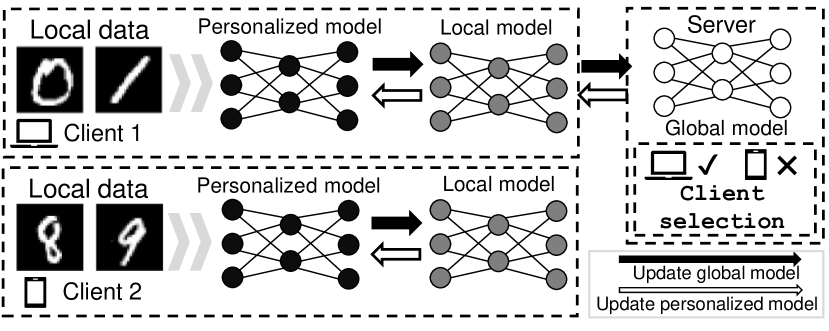
Figure 2: An example of FLAME. Various clients may own non-i.i.d. data. Selected clients download the global model from the server, and update their personalized models and local models, while unselected clients keep their model parameters unchanged. Client selection is performed on the server, and update messages uploaded by clients are used to update the global model.

4.2 Algorithmic Design

In Algorithm 1, we introduce FLAME, a PFL framework employing ADMM for the resolution of Problem (7). Fig. 2 shows an example of our algorithm. In each communication round $t$, the server selects $s$ clients from the entire client pool to form $\mathcal{S}^{t}$ (Line 1) by using an unbiased or biased client selection strategy. The selected clients update their local parameters using Equations (9)-(11) (Lines 1-1). However, when $f_{i}$ is non-convex, obtaining a closed-form solution to Problem (9) may be challenging. Therefore, for Problem (9), we employ gradient descent to iteratively update the personalized model until we get an $\epsilon_{i}^{t}$-approximate solution, which means

$$\begin{split}&||\nabla_{\boldsymbol{\theta}_{i}}\mathcal{L}(\boldsymbol{\theta}_{i}^{t+1},\boldsymbol{w}_{i}^{t},\boldsymbol{\pi}_{i}^{t},\boldsymbol{w}^{t})||^{2}\\ =&||\alpha_{i}(\nabla f_{i}(\boldsymbol{\theta}_{i}^{t+1})+\lambda(\boldsymbol{\theta}_{i}^{t+1}-\boldsymbol{w}_{i}^{t})||^{2}\leq\epsilon_{i}^{t}.\end{split}$$ (13)

Note that Equation (13) can be satisfied after $H:=\mathcal{O}(\nu\log(\frac{d}{\epsilon^{t}_{i}}))$ iterations, where $\nu$ is a condition number measuring the difficulty of optimizing Problem (9), $d$ is the diameter of the search space [5]. For clients not included in $\mathcal{S}^{t}$, their local parameters remain unchanged (Line 1). After the completion of local parameter updates for each client, the update messages $z_{i}^{t+1}$, $i\in[m]$ are sent to the server for updating the global model (Lines 1 and 1).

4.3 Biased Client Selection

Motivated by [7], we propose a biased client selection strategy in the context of PFL, with the goal of speeding up the convergence. Cho et al. [7] proposed to select clients with higher loss before each communication to accelerate the convergence of FedAvg [32], and they established theoretical convergence analysis based on this concept. Unlike FedAvg, FLAME is a primal-dual PFL framework. Our theoretical analysis in Section 4.4 indicates that choosing clients with larger personalized model update magnitudes, i.e., $||\boldsymbol{\theta}_{i}^{t+1}-\boldsymbol{\theta}_{i}^{t}||^{2}$, can speed up the convergence. However, in the practical context of PFL, quantifying the personalized model update magnitudes is challenging. This issue arises due to the fact that the updates to the personalized model occur subsequent to the client selection phase. However, we aim to ascertain superior-quality clients prior to the training of the personalized model. To address this issue, we propose to employ gradients as a metric to quantify the personalized model update magnitudes.

Theorem 1.

When $f_{i}$ is convex, or nonconvex but $\lambda$ is sufficiently large (such that $\mathcal{L}_{i}$ is $\mu$-strongly convex with respect to $\boldsymbol{\theta}_{i}$), the personalized model update magnitudes is approximately bounded by

$$\frac{1}{2\alpha_{i}^{2}(L^{2}+\lambda^{2})}|| \nabla_{\boldsymbol{\theta}_{i}}\mathcal{L}_{i}(\boldsymbol{\theta}_{i}^{t},\boldsymbol{w}_{i}^{t},\boldsymbol{\pi}_{i}^{t},\boldsymbol{w}^{t})||^{2}\leq||\boldsymbol{\theta}_{i}^{t+1}-\boldsymbol{\theta}_{i}^{t}||^{2}$$

$$\leq\frac{1}{\mu^{2}}||\nabla_{\boldsymbol{\theta}_{i}}\mathcal{L}_{i}(\boldsymbol{\theta}_{i}^{t},\boldsymbol{w}_{i}^{t},\boldsymbol{\pi}_{i}^{t},\boldsymbol{w}^{t})||^{2}.$$ (14)

The proof of Theorem 1 is provided in Appendix B. According to Theorem 1, both the upper and lower bounds of $||\boldsymbol{\theta}_{i}^{t+1}-\boldsymbol{\theta}_{i}^{t}||^{2}$ are bounded by $||\nabla_{\boldsymbol{\theta}_{i}}\mathcal{L}_{i}(\boldsymbol{\theta}_{i}^{t},\boldsymbol{w}_{i}^{t},\boldsymbol{\pi}_{i}^{t},\boldsymbol{w}^{t})||^{2}$, allowing us to estimate $||\boldsymbol{\theta}_{i}^{t+1}-\boldsymbol{\theta}_{i}^{t}||^{2}$ using $||\nabla_{\boldsymbol{\theta}_{i}}\mathcal{L}_{i}(\boldsymbol{\theta}_{i}^{t},\boldsymbol{w}_{i}^{t},\boldsymbol{\pi}_{i}^{t},\boldsymbol{w}^{t})||^{2}$. However, computing $\nabla_{\boldsymbol{\theta}_{i}}\mathcal{L}_{i}(\boldsymbol{\theta}_{i}^{t},\boldsymbol{w}_{i}^{t},\boldsymbol{\pi}_{i}^{t},\boldsymbol{w}^{t})$ is not only time-consuming but also challenging under constrained client computing conditions, such as limited RAM. When the size of the local dataset $X_{i}$ is significantly large, computing $\nabla_{\boldsymbol{\theta}_{i}}\mathcal{L}_{i}(\boldsymbol{\theta}_{i}^{t},\boldsymbol{w}_{i}^{t},\boldsymbol{\pi}_{i}^{t},\boldsymbol{w}^{t})$ requires a substantial amount of RAM and is exceedingly time-consuming. Therefore, we uniformly select a batch of data to compute $g_{i}$ for estimating $\nabla_{\boldsymbol{\theta}_{i}}\mathcal{L}_{i}(\boldsymbol{\theta}_{i}^{t},\boldsymbol{w}_{i}^{t},\boldsymbol{\pi}_{i}^{t},\boldsymbol{w}^{t})$, as it holds that $\mathbb{E}[g_{i}]=\nabla_{\boldsymbol{\theta}_{i}}\mathcal{L}_{i}(\boldsymbol{\theta}_{i}^{t},\boldsymbol{w}_{i}^{t},\boldsymbol{\pi}_{i}^{t},\boldsymbol{w}^{t})$ (Lines 1 and 1 in Algorithm 1) .

4.4 Convergence Analysis

Assumption 1 (Gradient Lipschitz continuity).

The expected loss function $f_{i}$ is $L$-smooth (gradient Lipschitz continue), i.e., for $\forall\boldsymbol{\theta}_{1},\boldsymbol{\theta}_{2}$, the following inequality holds

$$\|\nabla f_{i}(\boldsymbol{\theta}_{1})-\nabla f_{i}(\boldsymbol{\theta}_{2})\|\leq L\|\boldsymbol{\theta}_{1}-\boldsymbol{\theta}_{2}\|.$$ (15)

Note that Assumption 1 is generally satisfied for most commonly used machine learning models, such as Support Vector Machines (SVM), Multinomial Logistic Regression (MLR), Multi-layer Perceptrons (MLP), Convolutional Neural Networks (CNN), etc.

Lemma 1.

Let ${(\Theta^{t},W^{t},\Pi^{t},\boldsymbol{w}^{t})}$ denote the sequence generated by Algorithm 1, $\mathcal{L}^{t}\equiv\mathcal{L}(\Theta^{t},W^{t},\Pi^{t},\boldsymbol{w}^{t})$ represent the Lagrangian function value at the $t$-th iteration, and $\frac{\lambda^{2}\alpha_{i}^{2}(1+\rho)}{\rho^{2}}<\frac{\lambda\alpha_{i}+\rho}{2}$. If Assumption 1 holds for all $t\geq 0$, then it holds that

$$\mathcal{L}^{t+1}-\mathcal{L}^{t}\leq\sum_{i\in\mathcal{S}^{t}}\Big{(}\frac{\lambda^{2}\alpha_{i}^{2}(1+\rho)}{\rho^{2}}-\frac{\lambda\alpha_{i}+\rho}{2}\Big{)}\times$$

$$\big{(}||\boldsymbol{w}_{i}^{t+1}\!-\!\boldsymbol{w}_{i}^{t}||^{2}\!+\!||\boldsymbol{\theta}_{i}^{t+1}-\boldsymbol{\theta}_{i}^{t}||^{2}\big{)}\!+\!\frac{\alpha_{i}^{2}}{(\frac{1}{\rho^{2}}-1)\lambda^{2}\alpha_{i}^{2}-\frac{L\alpha_{i}+\rho}{2}}\epsilon_{i}^{t}.$$ (16)

The proof of Lemma 1 is given in Appendix C. Note that Lemma 1 is a key lemma for our convergence analysis.

Definition 2 (Relative Skew).

For any $i\in\mathcal{S}(\kappa,\boldsymbol{\theta}_{i})$, we define

$$\gamma(\mathcal{S}(\kappa,\boldsymbol{\theta}_{i}),\boldsymbol{\theta}_{i}^{{}^{\prime}})\!:=\!\frac{\mathbb{E}_{\mathcal{S}(\kappa,\boldsymbol{\theta}_{i})}[\frac{1}{|\mathcal{S}(\kappa,\boldsymbol{\theta}_{i})|}\!\sum_{i\in\mathcal{S}(\kappa,\boldsymbol{\theta}_{i})}||\boldsymbol{\theta}_{i}^{{}^{\prime}}-\boldsymbol{\theta}_{i}||^{2}]}{\frac{1}{m}\sum_{i=1}^{m}||\boldsymbol{\theta}_{i}^{{}^{\prime}}-\boldsymbol{\theta}_{i}||^{2}},$$ (17)

which reflects the skew of a client selection strategy $\kappa$, $\boldsymbol{\theta}_{i}$ in $\mathcal{S}(\kappa,\boldsymbol{\theta}_{i})$ represents the dominantly personalized model in client selection, $\boldsymbol{\theta}_{i}^{{}^{\prime}}$ represents the model to be evaluated. When employing the unbiased client selection strategy $\kappa$, it is trivial to show that $\gamma(\mathcal{S}(\kappa,\boldsymbol{\theta}_{i}),\boldsymbol{\theta}_{i}^{{}^{\prime}})=1$. Here we define a related metric that is independent of $\boldsymbol{\theta}_{i}$ and $\boldsymbol{\theta}^{{}^{\prime}}$. This metric enables us to obtain the convergence analysis for the biased client selection strategy:

$$\overline{\gamma}=\min_{\boldsymbol{\theta}_{i},\boldsymbol{\theta}_{i}^{{}^{\prime}}}\gamma\big{(}\mathcal{S}(\kappa,\boldsymbol{\theta}_{i}),\boldsymbol{\theta}_{i}^{{}^{\prime}}\big{)}.$$ (18)

According to Equation (17), it is not difficult to deduce that when selecting clients with larger values of $||\boldsymbol{\theta}_{i}^{{}^{\prime}}-\boldsymbol{\theta}_{i}||^{2}$, the value of $\overline{\gamma}$ becomes larger. Next, we present the main theorem which establishes the convergence under both unbiased and biased client selection strategies.

Theorem 2.

Let $\mathcal{P}^{t}={(\Theta^{t},W^{t},\Pi^{t},\boldsymbol{w}^{t})}$ denote the sequence generated by Algorithm 1, $\frac{\lambda^{2}\alpha_{i}^{2}(1+\rho)}{\rho^{2}}<\frac{\lambda\alpha_{i}+\rho}{2}$, $\rho\geq\lambda\alpha_{i}$, and $\epsilon_{\text{max}}=\max_{i,t}\epsilon_{i}^{t}$ for each client $i\in[m]$. It holds that

1) when employing the unbiased client selection strategy, then

$$\frac{1}{mT}\sum_{t=0}^{T-1}||\nabla\mathcal{L}(\mathcal{P}^{t})||^{2}\leq\frac{1}{sT}\frac{c_{2}}{c_{1}}\mathbb{E}[\mathcal{L}^{0}\!-\!\mathcal{L}^{t+1}]\!+\!c_{3}\epsilon_{\max},$$ (19)

2) when employing a biased client selection strategy, then

$$\frac{1}{mT}\sum_{t=0}^{T-1}||\nabla\mathcal{L}(\Theta^{t})||^{2}\leq\frac{1}{sT}\frac{c_{2}}{c_{1}\overline{\gamma}}\mathbb{E}[\mathcal{L}^{0}\!-\!\mathcal{L}^{t+1}]\!+\!c_{4}\epsilon_{\max},$$ (20)

where

$$\begin{split}&||\nabla\mathcal{L}(\mathcal{P}^{t})||^{2}:=||\nabla_{\boldsymbol{w}}\mathcal{L}(\mathcal{P}^{t})||^{2}+\quad\quad\quad\quad\quad\quad\quad\quad\\ &\sum_{i=1}^{m}||\nabla_{\boldsymbol{\theta}_{i}}\mathcal{L}(\mathcal{P}^{t})||^{2}+||\nabla_{\boldsymbol{w}_{i}}\mathcal{L}(\mathcal{P}^{t})||^{2}+||\nabla_{\boldsymbol{\pi}_{i}}\mathcal{L}(\mathcal{P}^{t})||^{2},\\ &||\nabla\mathcal{L}(\Theta^{t})||^{2}:=\!\sum_{i=1}^{m}||\nabla_{\boldsymbol{\theta}_{i}}\mathcal{L}(\mathcal{P}^{t})||^{2},\\ &c_{0}=\max_{i}\frac{\alpha_{i}^{2}}{(\frac{1}{\rho^{2}}-1)\lambda^{2}\alpha_{i}^{2}-\frac{L\alpha_{i}+\rho}{2}},\\ &c_{1}=\min_{i}\frac{\lambda\alpha_{i}+\rho}{2}-\frac{\lambda^{2}\alpha_{i}^{2}(1+\rho)}{\rho^{2}},\\ &c_{2}=4\lambda^{2}\alpha_{\max}^{2}(1+\frac{1}{\rho^{2}})+2\alpha_{\max}^{2}(L^{2}+2\lambda^{2})+2\rho^{2}+2,\\ &c_{3}=2+\frac{c_{2}c_{0}}{c_{1}},\text{ }c_{4}=2+\frac{mc_{0}c_{2}}{sc_{1}\overline{\gamma}}.\end{split}$$

The full proof of Theorem 2 is given in Appendix D. According to Theorem 2, we obtain the summation of $||\nabla\mathcal{L}(\mathcal{P}^{t})||^{2}$ and $||\nabla\mathcal{L}(\Theta^{t})||^{2}$ vanish with a convergence rate of $\mathcal{O}(\frac{1}{T})$, which is considered sub-linear. It is worth noting that this convergence rate is established solely under Assumption 1, which pertains to gradient Lipschitz continuity, a condition that is not hard to satisfy. In contrast, the result in [44] is obtained under more assumptions, including gradient Lipschitz continuity, bounded variance, and bounded diversity. Moreover, a noteworthy insight from Theorem 2 is that a larger relative skew $\overline{\gamma}$ leads to a faster convergence rate of $\mathcal{O}(\frac{1}{\overline{\gamma}T})$. This insight implies that selecting clients with larger personalized model update magnitudes can speed up the convergence of the personalized model. In our numerical evaluations, we observe that the biased client selection strategy not only accelerates the convergence of the personalized models but also speeds up the convergence of the global model.

5 Experiments

TABLE I: An overview of the datasets and models.

Datasets	# of samples	Ref.	Models	# of parameters
Synthetic	5k-10k/device	[28]	SVM	610/device
Mnist	70,000	[22]	MLR	7,850/device
Fmnist	70,000	[50]	MLP	79,510/device
Mmnist	58,954	[1]	CNN	206,678/device

Goals.  In the experiments, we aim to evaluate the performance of FLAME in comparison to other methods and investigate how different parameters influence the effectiveness of FLAME. Moreover, we evaluate whether the biased client selection strategy can speed up convergence.

5.1 Settings

Datasets.  To evaluate the performance of FLAME, we conducted evaluations on three real-world datasets and a synthetic dataset. For the real-world datasets, we employ the widely used Mnist [22], Fashion MNIST (Fmnist) [50], and Medical Mnist (Mmnist) [1]. To accommodate data heterogeneity, we organize the training data by their labels and distribute them into shards, with each client being assigned two shards randomly. For the synthetic dataset (Synthetic), we adopted a setup similar to [27], which generates 60-dimensional random vectors as input heterogeneous data.

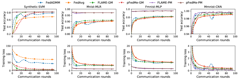
Figure 3: A comparison of the training loss and test accuracy across different methods. The dashed lines represent the global models, while the solid lines represent the personalized models.

TABLE II: A comparison of accuracy among different approaches with 50 and 100 clients. In each column, the two bold values respectively represent the highest accuracy achieved by the personalized model and the global model.

Methods	50 clients (Accuracy%)					100 clients (Accuracy%)
	Synthetic-SVM	Mnist-MLR	Fmnist-MLP	Mmnist-CNN		Synthetic-SVM	Mnist-MLR	Fmnist-MLP	Mmnist-CNN
FLAME-PM	82.07$\pm$0.03	97.14$\pm$0.02	96.37$\pm$0.02	99.80$\pm$0.01		81.97$\pm$0.01	97.87$\pm$0.02	96.02$\pm$0.03	99.72$\pm$0.01
FLAME-GM	81.90$\pm$0.02	91.12$\pm$0.03	82.76$\pm$0.01	99.36$\pm$0.02		73.09$\pm$0.01	90.64$\pm$0.02	80.90$\pm$0.02	99.25$\pm$0.02
pFedMe-PM	82.01$\pm$0.01	97.03$\pm$0.01	96.39$\pm$0.02	99.76$\pm$0.01		81.93$\pm$0.01	96.90$\pm$0.02	95.96$\pm$0.01	99.65$\pm$0.01
pFedMe-GM	81.72$\pm$0.02	90.69$\pm$0.02	82.29$\pm$0.04	99.02$\pm$0.02		67.91$\pm 0.02$	90.29$\pm$0.01	80.30$\pm$0.02	98.95$\pm$0.01
FedAvg	68.64$\pm$0.01	90.23$\pm$0.01	81.28$\pm$0.02	99.22$\pm$0.03		56.27$\pm$0.02	90.28$\pm$0.01	81.10$\pm$0.01	98.80$\pm$0.02
FedADMM	79.02$\pm$0.02	90.67$\pm$0.04	82.63$\pm$0.04	99.47$\pm$0.03		67.13$\pm$0.02	90.19$\pm$0.03	81.83$\pm$0.03	99.12$\pm$0.02

TABLE III: Comparison of communication rounds among different methods when reaching the specified accuracy level.

Methods	50 clients (Communication rounds)
	Synthetic-SVM	Mnist-MLR	Fmnist-MLP	Mmnist-CNN
FedAvg	63	94	56	15
FedADMM	6 (10.5$\times$)	9 (10.4$\times$)	44 (1.3$\times$)	10 (1.5$\times$)
FLAME	9 (7.0$\times$)	21 (4.5$\times$)	28 (2.0$\times$)	10 (1.5$\times$)
pFedMe	23 ($2.7\times$)	88 (1.1$\times$)	51 (1.1$\times$)	15

Models.  We analyze four datasets in both convex and non-convex scenarios. Specifically, we use SVM for Synthetic, MLR for Mnist, MLP for Fmnist, and CNN for Mmnist. A comprehensive overview of the datasets and models is presented in Table I.

Baselines.  We experimentally evaluate the performance of FLAME against three methods, namely, pFedMe [44], FedADMM [12], and FedAvg [32]. As explained in our related work, pFedMe is the state-of-the-art PFL approach. FedADMM and FedAvg are two approaches that perform centralized FL without personalized models: FedADMM is a primal-dual FL approach that can mitigate the impact of data heterogeneity on training models. To evaluate the performance of models under different methods and parameters, we employ training loss and test accuracy as metrics. We use FLAME-GM as an abbreviation for the global model of FLAME and FLAME-PM as an abbreviation for the personalized model of FLAME. Similarly, pFedMe-GM and pFedMe-PM follow the same convention.

Implementations.  Our algorithms were executed on a computational platform comprising two Intel Xeon Gold 5320 CPUs with 52 cores, 512 GB of RAM, four NVIDIA A800 with 320 GB VRAM and operating on the Ubuntu 22.04 environment. The software implementation was realized in Python 3.8 and Pytorch 2.1, and open-sourced.

5.2 Numerical Comparisons

5.2.1 Comparison of multiple methods

Fig. 3 illustrates how the test accuracy and training loss vary with the number of communication rounds for different methods. We configured each method with a local learning rate $\eta=0.01$, a batch size of 100, and the number of clients $m$ set to 50. Additionally, for all subsequent experiments, we set $\alpha_{i}=1/m$. For FedADMM and FLAME, we set $\rho=0.01$, while for FLAME and pFedMe, we set $\lambda=5$, with local iterations $H=5$. For pFedMe, we select the best-performing learning rate for its global model from the candidate set $\{0.01,0.05,0.1,0.2,0.5\}$. Table II presents the comparison of the highest accuracy achieved by different methods with 50 and 100 clients, respectively. Table III presents the communication rounds required for the global model to converge to the specified accuracy for various methods. We set specified accuracy for four datasets and their respective models as follows: 65%, 90%, 80%, and 98%.

Observations. According to Fig. 3, we observe that the convergence rate of FLAME’s global model is only slower than FedADMM in the initial communication rounds. However, as the number of communication rounds increases, FLAME demonstrates the ability to converge to a superior local optimum compared to all other methods. Regarding personalized models, FLAME and pFedMe exhibit comparable performance in Synthetic, Mnist, and Fmnist datasets, with FLAME outperforming pFedMe in the case of Mmnist. Table II indicates that, in most scenarios, FLAME achieves the highest accuracy for both personalized and global models. Additionally, Table III reveals that FLAME requires the fewest communication rounds to reach the specified accuracy on Fmnist and Mmnist, whereas FedADMM requires the fewest rounds for Synthetic and Mnist datasets, though it falls short of achieving FLAME’s highest accuracy.

5.2.2 Effect of regularization $\lambda$

Fig. 4 illustrates the impact of different regularization parameters $\lambda$ on convergence. We configured the local learning rate $\eta$ to be 0.01, the penalty parameter $\rho$ to be 0.01, and the number of local iterations $H$ to be 5. We set $\lambda$ to 1, 3, 5, respectively, to observe how the losses of personalized models and global model in FLAME vary with communication rounds.

Observations. From Fig. 4, we observe that as the value of $\lambda$ increases, the personalized model converges more slowly, while the global model converges faster. This is attributed to the fact that an increase in the regularization parameter $\lambda$, results in a stronger penalty on minimizing the disparity between the personalized model and the global model. Consequently, this causes the personalized model to approach the global model more closely.

5.2.3 Effect of local iterations $H$

Fig. 5 illustrates the impact of different local iterations $H$ on the convergence of FLAME. We configured the local learning rate $\eta$ to be 0.01, the penalty parameter $\rho$ to be 0.01, and the regularization parameter $\lambda$ to be 5. We set $H$ to 1, 5, 10, respectively, to observe the changes in the loss of FLAME’s personalized models and global model as communication rounds vary.

Observations. From Fig. 5, it is evident that increasing local iterations significantly accelerates the convergence of FLAME. This is due to the improved precision in solving the personalized model $\boldsymbol{\theta}_{i}$ with the growth of local iterations, a characteristic inherent to the first-order gradient method. The enhanced accuracy of the personalized model, in turn, improves the precision of solving the dual variables $\boldsymbol{\pi}_{i}$ and the global model $\boldsymbol{w}$, resulting in accelerated convergence of both the global and personalized models. However, as the number of local iterations increases beyond a certain threshold, the performance of both the personalized and global models stabilizes. For example, the performance on Synthetic remains nearly identical when $H=3$ and $H=5$.

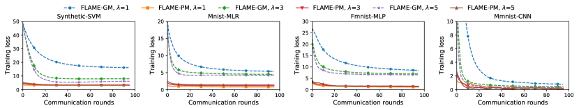
Figure 4: Effect of the regularization parameter $\lambda$ on the convergence of FLAME. As $\lambda$ increases, the performance of the personalized models becomes closer to that of the global models.

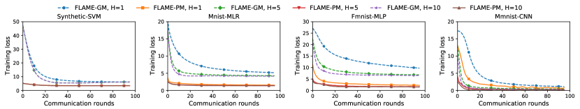
Figure 5: Effect of the local iterations $H$ on the convergence of FLAME. As $H$ increases, the performance of personalized and global models improves.

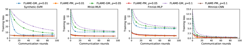
Figure 6: Effect of the penalty parameter $\rho$ on the convergence of FLAME. As $\rho$ decreases, the performance of the personalized models and the global models improves.

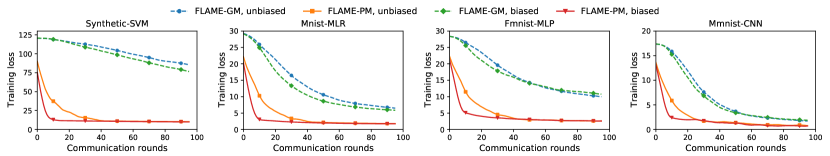
Figure 7: Effect of the biased client selection strategy on the convergence of FLAME. Biased client selection strategy converges faster than unbiased client selection strategy.

5.2.4 Effect of penalty $\rho$

Fig. 6 illustrates the impact of different values of the penalty parameter $\rho$ on the convergence of FLAME. We set the local learning rate $\eta$ to 0.01, regularization parameter $\lambda$ to 5, and local iterations $H$ to 5. We vary $\rho$ values as 0.01, 0.05, and 0.1 to observe changes in the loss of FLAME’s personalized models and the global model with respect to communication rounds.

Observations. From Fig. 6, it is evident that reducing $\rho$ accelerates the convergence of FLAME. This is because with increasing $\rho$, the penalty between the local and global models becomes more stringent, pushing the local model closer to the global model and further away from the better-performing personalized model. Consequently, this slows down the convergence of both the personalized models and the global model.

5.2.5 Effect of biased client selection

Fig. 7 illustrates the impact of different client selection strategies on the convergence of FLAME. We set the local learning rate to $\eta=0.01$, regularization parameter to $\lambda=5$, local iterations to $H=5$, penalty parameter to $\rho=0.01$, the number of clients to $m=100$, the size of the candidate clients set $\mathcal{C}^{t}$ to 50, and the size of the selected client set $\mathcal{S}^{t}$ to 10. We examine how the loss of personalized models and the global model in FLAME change with communication rounds under two strategies: unbiased and biased client selection.

Observations. Fig. 7 reveals that, across the four datasets, the biased client selection strategy significantly expedites the convergence of both global and personalized models compared to the unbiased client selection strategy. This validates that our proposed biased client selection strategy can not only expedite the convergence of personalized models, but also accelerate the convergence of global model.

5.2.6 Summary of Lessons Learned

• In comparison with multiple methods, we observed that FLAME converges faster than state-of-the-art methods. Furthermore, FLAME outperforms other methods in training models on heterogeneous data, specifically by achieving higher accuracy and lower loss. In terms of communication performance, FLAME achieves an average acceleration of 3.75$\times$ compared to FedAvg.

• Choosing appropriate parameters can significantly enhance the performance of FLAME. The regularization parameter $\lambda$ can adjust the gap between personalized and global models, with a larger $\lambda$ narrowing the gap between them. Increasing local iterations can improve model accuracy, thus expediting convergence. Reducing the penalty parameter can make local models lean more toward higher-accuracy personalized models, thereby accelerating convergence. Due to the fact that FLAME does not require the adjustment of learning rate when training the global model, it significantly reduces the burden of hyperparameter tuning in comparison to pFedMe.

• Our experiments have validated that the biased client selection strategy can expedite the convergence of FLAME. This acceleration is evident not only in the personalized model but also in the global model. Consequently, the communication efficiency of FLAME can be improved by adopting the biased client selection strategy.

6 Conclusion and Future Work

In this paper, we proposed a PFL framework, FLAME. We formulated the optimization problem for PFL based on the Moreau envelope and solved it using the ADMM. Additionally, we proposed a biased client selection strategy to speed up the convergence. Our theoretical analysis demonstrated that FLAME achieves a sub-linear convergence rate. Our experimental results demonstrated the superior performance of our approach in training models on heterogeneous data when compared to state-of-the-art methods. Furthermore, FLAME, when applied to solving the global model, eliminates the need for learning rate adjustments, thereby significantly alleviating the burden of hyperparameter tuning in contrast to pFedMe. This attribute positions FLAME as a highly promising candidate for applications such as next-word prediction and training LLM.

In the future, we will focus on addressing privacy issues in PFL, with an emphasis on using techniques such as encryption and differential privacy to mitigate privacy leakages.

Shengkun Zhu received the BE degree in electronic information engineering from Dalian University of Technology (DUT), China in 2018. He is currently working toward a Ph.D. degree in computer science and technology, School of Computer Science, Wuhan University, China. His research interests mainly include federated learning and nonconvex optimization.

Jinshan Zeng received the Ph.D. degree in mathematics from Xi’an Jiaotong University, Xi’an, China, in 2015. He is currently a Distinguished Professor with the School of Computer and Information Engineering, Jiangxi Normal University, Nanchang, China, and serves as the Director of the Department of Data Science and Big Data. He has authored more than 40 papers in high-impact journals and conferences such as IEEE TPAMI, JMLR, IEEE TSP, ICML, and AAAI. He has coauthored two papers with collaborators that received the International Consortium of Chinese Mathematicians (ICCM) Best Paper Award in 2018 and 2020). His current research interests include nonconvex optimization, machine learning (in particular deep learning), and remote sensing.

Sheng Wang received the BE degree in information security, ME degree in computer technology from Nanjing University of Aeronautics and Astronautics, China in 2013 and 2016, and Ph.D. from RMIT University in 2019. He is a professor at the School of Computer Science, Wuhan University. His research interests mainly include spatial databases. He has published full research papers on top database and information systems venues as the first author, such as TKDE, SIGMOD, PVLDB, and ICDE.

Yuan Sun is a Lecturer in Business Analytics and Artificial Intelligence at La Trobe University, Australia. He received his BSc in Applied Mathematics from Peking University, China, and his PhD in Computer Science from The University of Melbourne, Australia. His research interest is on artificial intelligence, machine learning, operations research, and evolutionary computation. He has contributed significantly to the emerging research area of leveraging machine learning for combinatorial optimisation. His research has been published in top-tier journals and conferences such as IEEE TPAMI, IEEE TEVC, EJOR, NeurIPS, ICLR, VLDB, ICDE, and AAAI.

Zhiyong Peng received the BSc degree from Wuhan University, in 1985, the MEng degree from the Changsha Institute of Technology of China, in 1988, and the PhD degree from the Kyoto University of Japan, in 1995. He is a professor of computer school, the Wuhan University of China. He worked as a researcher in Advanced Software Technology & Mechatronics Research Institute of Kyoto from 1995 to 1997 and a member of technical staff in Hewlett-Packard Laboratories Japan from 1997 to 2000. His research interests include complex data management, web data management, and trusted data management. He is a member of IEEE Computer Society, ACM SIGMOD and vice director of Database Society of Chinese Computer Federation. He was general co-chair of WAIM 2011, DASFAA 2013 and PC Co-chair of DASFAA 2012, WISE 2006, and CIT 2004.

Appendix A Some Useful Properties

We provide a list of useful properties and lemmas that are necessary for proving our theorems. Proposition 2 provides an exposition of a property of smooth function, while Proposition 3 presents commonly employed Jensen’s inequalities. Lemmas 2 and 3 will be employed in the proof of our main theorem.

Proposition 2.

For any $L$-smooth function $f$ and $\boldsymbol{\theta}_{i}$, $i=1,2$, we have

$$f(\boldsymbol{\theta}_{1})-f(\boldsymbol{\theta}_{2})-\langle\nabla f(\boldsymbol{\theta}_{i}),\boldsymbol{\theta}_{1}-\boldsymbol{\theta}_{2}\rangle\leq\frac{L}{2}||\boldsymbol{\theta}_{1}-\boldsymbol{\theta}_{2}||^{2}.$$ (21)

Proposition 3 (Jensen’s inequalities).

For any vectors $\boldsymbol{\theta}_{1}$, $\boldsymbol{\theta}_{2}$ and $k>0$, we have

$$2\langle\boldsymbol{\theta}_{1},\boldsymbol{\theta}_{2}\rangle \leq k||\boldsymbol{\theta}_{1}||^{2}+\frac{1}{k}||\boldsymbol{\theta}_{2}||^{2},$$ (22)

$$||\boldsymbol{\theta}_{1}-\boldsymbol{\theta}_{2}||^{2} \leq(1+k)||\boldsymbol{\theta}_{1}||^{2}+(1+\frac{1}{k})||\boldsymbol{\theta}_{2}||^{2},$$ (23)

$$||\sum_{i=1}^{m}\boldsymbol{\theta}_{i}||^{2} \leq m\sum_{i=1}^{m}||\boldsymbol{\theta}_{i}||^{2}.$$ (24)

Lemma 2.

For any $t\geq 0$, the following equation holds

$$\begin{split}\boldsymbol{\pi}_{i}^{t}=\lambda\alpha_{i}(\boldsymbol{\theta}_{i}^{t}-\boldsymbol{w}_{i}^{t}).\end{split}$$ (25)

Proof.

Transposing Equation (10) yields:

$$\boldsymbol{\pi}_{i}^{t}=\lambda\alpha_{i}\boldsymbol{\theta}_{i}^{t+1}+\rho\boldsymbol{w}^{t}-(\lambda\alpha_{i}+\rho)\boldsymbol{w}_{i}^{t+1}.$$ (26)

We first establish the case when $t\geq 1$. Substituting Equation (26) into Equation (11), we obtain:

$$\boldsymbol{\pi}_{i}^{t+1} =\boldsymbol{\pi}_{i}^{t}+\rho(\boldsymbol{w}_{i}^{t+1}-\boldsymbol{w}^{t})$$

$$=\lambda\alpha_{i}(\boldsymbol{\theta}_{i}^{t+1}-\boldsymbol{w}_{i}^{t+1}).$$ (27)

Next we establish the case when $t=0$ by initializing the parameters as

$$\boldsymbol{\pi}_{i}^{0}=\lambda\alpha_{i}(\boldsymbol{\theta}_{i}^{0}-\boldsymbol{w}_{i}^{0}).$$ (28)

Combine the two cases, then we have

$$\boldsymbol{\pi}_{i}^{t}=\lambda\alpha_{i}(\boldsymbol{\theta}_{i}^{t}-\boldsymbol{w}_{i}^{t}),t\geq 0.$$ (29)

∎

Lemma 3.

When $\rho\geq\lambda\alpha_{i}$ for each client $i\in[m]$, the Lagrangian function value in the $(t+1)$-th iteration is lower bounded as $\mathcal{L}^{t+1}\geq F^{*}$, where $F^{*}=\min_{\boldsymbol{w},\boldsymbol{\theta}_{i}}\sum_{i=1}^{m}\alpha_{i}\left(f_{i}(\boldsymbol{\theta}_{i})+\frac{\lambda}{2}||\boldsymbol{\theta}_{i}-\boldsymbol{w}||^{2}\right)$.

Proof.

According to Equation (8), we obtain

$$\mathcal{L}^{t+1} =\sum_{i=1}^{m}\alpha_{i}(f_{i}(\boldsymbol{\theta}_{i}^{t+1})+\frac{\lambda}{2}||\boldsymbol{\theta}_{i}^{t+1}-\boldsymbol{w}_{i}^{t+1}||^{2})+$$

$$\quad\quad\langle\boldsymbol{\pi}_{i}^{t+1},\boldsymbol{w}_{i}^{t+1}-\boldsymbol{w}^{t+1}\rangle+\frac{\rho}{2}||\boldsymbol{w}_{i}^{t+1}-\boldsymbol{w}^{t+1}||^{2}$$

$$=\sum_{i=1}^{m}\alpha_{i}(f_{i}(\boldsymbol{\theta}_{i}^{t+1})+\frac{\lambda}{2}||\boldsymbol{\theta}_{i}^{t+1}-\boldsymbol{w}_{i}^{t+1}||^{2})+$$

$$\quad\quad\frac{\lambda\alpha_{i}}{2}\langle 2\boldsymbol{\theta}_{i}^{t+1}-\boldsymbol{w}_{i}^{t+1}-\boldsymbol{w}^{t+1},\boldsymbol{w}_{i}^{t+1}-\boldsymbol{w}^{t+1}\rangle-$$

$$\quad\quad\frac{\lambda\alpha_{i}}{2}\langle 2\boldsymbol{\theta}_{i}^{t+1}-\boldsymbol{w}_{i}^{t+1}-\boldsymbol{w}^{t+1},\boldsymbol{w}_{i}^{t+1}-\boldsymbol{w}^{t+1}\rangle+$$

$$\quad\quad\langle\boldsymbol{\pi}_{i}^{t+1},\boldsymbol{w}_{i}^{t+1}-\boldsymbol{w}^{t+1}\rangle+\frac{\rho}{2}||\boldsymbol{w}_{i}^{t+1}-\boldsymbol{w}^{t+1}||^{2}$$

$$=\sum_{i=1}^{m}\alpha_{i}(f_{i}(\boldsymbol{\theta}_{i}^{t+1})+\frac{\lambda}{2}||\boldsymbol{\theta}_{i}^{t+1}-\boldsymbol{w}^{t+1}||^{2})-$$

$$\quad\quad\frac{\lambda\alpha_{i}}{2}\langle 2\boldsymbol{\theta}_{i}^{t+1}-\boldsymbol{w}_{i}^{t+1}-\boldsymbol{w}^{t+1},\boldsymbol{w}_{i}^{t+1}-\boldsymbol{w}^{t+1}\rangle+$$

$$\quad\quad\langle\lambda\alpha_{i}(\boldsymbol{\theta}_{i}^{t+1}-\boldsymbol{w}_{i}^{t+1}),\boldsymbol{w}_{i}^{t+1}-\boldsymbol{w}^{t+1}\rangle+$$

$$\quad\quad\frac{\rho}{2}||\boldsymbol{w}_{i}^{t+1}-\boldsymbol{w}^{t+1}||^{2}$$

$$=\sum_{i=1}^{m}\alpha_{i}(f_{i}(\boldsymbol{\theta}_{i}^{t+1})+\frac{\lambda}{2}||\boldsymbol{\theta}_{i}^{t+1}-\boldsymbol{w}^{t+1}||^{2})+$$

$$\quad\quad\frac{\rho-\lambda\alpha_{i}}{2}||\boldsymbol{w}_{i}^{t+1}-\boldsymbol{w}^{t+1}||^{2}$$

$$\geq F^{*}+\sum_{i=1}^{m}\frac{\rho-\lambda\alpha_{i}}{2}||\boldsymbol{w}_{i}^{t+1}-\boldsymbol{w}^{t+1}||^{2}\geq F^{*},$$ (30)

where the first equality is due to Lagrangian function (8), the third equality is due to Lemma 2 and the equality

$$||\boldsymbol{a}-\boldsymbol{b}||^{2}=||\boldsymbol{a}-\boldsymbol{c}||^{2}+\langle 2\boldsymbol{a}-\boldsymbol{b}-\boldsymbol{c},\boldsymbol{c}-\boldsymbol{b}\rangle,$$

and the last inequality is due to the optimal condition. ∎

Appendix B Proof of Therorem 1

Proof.

Based on Lagrangian function (8), we obtain

$$||\nabla_{\boldsymbol{\theta}_{i}}\mathcal{L}_{i}(\boldsymbol{\theta}_{i}^{t+1},\boldsymbol{w}_{i}^{t},\boldsymbol{\pi}_{i}^{t},\boldsymbol{w}^{t})\!-\!\nabla_{\boldsymbol{\theta}_{i}}\mathcal{L}_{i}(\boldsymbol{\theta}_{i}^{t},\boldsymbol{w}_{i}^{t},\boldsymbol{\pi}_{i}^{t},\boldsymbol{w}^{t})||^{2}$$

$$= ||\alpha_{i}\left(\nabla_{\boldsymbol{\theta}_{i}}f_{i}(\boldsymbol{\theta}_{i}^{t+1})-\nabla_{\boldsymbol{\theta}_{i}}f_{i}(\boldsymbol{\theta}_{i}^{t})\right)+\alpha_{i}\lambda(\boldsymbol{\theta}_{i}^{t+1}-\boldsymbol{\theta}_{i}^{t})||^{2}$$

$$\leq 2\alpha_{i}^{2}||\nabla_{\boldsymbol{\theta}_{i}}f_{i}(\boldsymbol{\theta}_{i}^{t+1})-\nabla_{\boldsymbol{\theta}_{i}}f_{i}(\boldsymbol{\theta}_{i}^{t})||^{2}+2\alpha_{i}^{2}\lambda^{2}||\boldsymbol{\theta}_{i}^{t+1}-\boldsymbol{\theta}_{i}^{t}||^{2}$$

$$\leq 2\alpha_{i}^{2}(L^{2}+\lambda^{2})||\boldsymbol{\theta}_{i}^{t+1}-\boldsymbol{\theta}_{i}^{t}||^{2},$$ (31)

where the first inequality is due to Proposition (3), and the second inequality is due to the gradient Lipschitz continuity of $f_{i}$. When $\lambda$ is sufficiently large such that $L_{i}$ is $\mu$-strongly convex with respect to $\boldsymbol{\theta}_{i}$, we have

$$||\boldsymbol{\theta}_{i}^{t+1}-\boldsymbol{\theta}_{i}^{t}||^{2}\leq\frac{1}{\mu^{2}}\times$$

$$||\nabla_{\boldsymbol{\theta}_{i}}\mathcal{L}_{i}(\boldsymbol{\theta}_{i}^{t+1},\boldsymbol{w}_{i}^{t},\boldsymbol{\pi}_{i}^{t},\boldsymbol{w}^{t})\!-\!\nabla_{\boldsymbol{\theta}_{i}}\mathcal{L}_{i}(\boldsymbol{\theta}_{i}^{t},\boldsymbol{w}_{i}^{t},\boldsymbol{\pi}_{i}^{t},\boldsymbol{w}^{t})||^{2},$$ (32)

Based on our algorithmic design and the optimal conditions, we have

$$||\nabla_{\boldsymbol{\theta}_{i}}\mathcal{L}(\boldsymbol{\theta}_{i}^{t+1},\boldsymbol{w}_{i}^{t},\boldsymbol{\pi}_{i}^{t},\boldsymbol{w}^{t})||^{2}\leq\!\epsilon_{i}^{t}\ll\!||\nabla_{\boldsymbol{\theta}_{i}}\mathcal{L}(\boldsymbol{\theta}_{i}^{t},\boldsymbol{w}_{i}^{t},\boldsymbol{\pi}_{i}^{t},\boldsymbol{w}^{t})||^{2}.$$

Therefore, we can derive an approximation

$$\frac{1}{2\alpha_{i}^{2}(L^{2}+\lambda^{2})}|| \nabla_{\boldsymbol{\theta}_{i}}\mathcal{L}_{i}(\boldsymbol{\theta}_{i}^{t},\boldsymbol{w}_{i}^{t},\boldsymbol{\pi}_{i}^{t},\boldsymbol{w}^{t})||^{2}\leq||\boldsymbol{\theta}_{i}^{t+1}-\boldsymbol{\theta}_{i}^{t}||^{2}$$

$$\leq\frac{1}{\mu^{2}}||\nabla_{\boldsymbol{\theta}_{i}}\mathcal{L}_{i}(\boldsymbol{\theta}_{i}^{t},\boldsymbol{w}_{i}^{t},\boldsymbol{\pi}_{i}^{t},\boldsymbol{w}^{t})||^{2}.$$ (33)

∎

Appendix C Proof of Lemma 1

Proof.

We decompose the gap between $\mathcal{L}^{t+1}$ and $\mathcal{L}^{t}$ as

$$\mathcal{L}^{t+1}\!-\!\mathcal{L}^{t}\!=\!\mathcal{L}(\Theta^{t+1},W^{t+1},\Pi^{t+1},\boldsymbol{w}^{t+1})\!-\!\mathcal{L}(\Theta^{t},W^{t},\Pi^{t},\boldsymbol{w}^{t})$$

$$=\underbrace{\mathcal{L}(\Theta^{t+1},W^{t+1},\Pi^{t+1},\boldsymbol{w}^{t+1})\!-\!\mathcal{L}(\Theta^{t+1},W^{t+1},\Pi^{t+1},\boldsymbol{w}^{t})}_{e_{1}^{t}}$$

$$\quad+\underbrace{\mathcal{L}(\Theta^{t+1},W^{t+1},\Pi^{t+1},\boldsymbol{w}^{t})\!-\!\mathcal{L}(\Theta^{t+1},W^{t+1},\Pi^{t},\boldsymbol{w}^{t})}_{e_{2}^{t}}$$

$$\quad+\underbrace{\mathcal{L}(\Theta^{t+1},W^{t+1},\Pi^{t},\boldsymbol{w}^{t})\!-\!\mathcal{L}(\Theta^{t+1},W^{t},\Pi^{t},\boldsymbol{w}^{t})}_{e_{3}^{t}}$$

$$\quad+\underbrace{\mathcal{L}(\Theta^{t+1},W^{t},\Pi^{t},\boldsymbol{w}^{t})\!-\!\mathcal{L}(\Theta^{t},W^{t},\Pi^{t},\boldsymbol{w}^{t})}_{e_{4}^{t}}.$$ (34)

Next, we individually estimate $e_{1}^{t}$, $e_{2}^{t}$, $e_{3}^{t}$, and $e_{4}^{t}$.

Estimate of $e_{1}^{t}$. Using the Lagrangian function, we have

$$e_{1}^{t} =\sum_{i=1}^{m}\langle\boldsymbol{\pi}_{i}^{t+1},\boldsymbol{w}_{i}^{t+1}-\boldsymbol{w}^{t+1}\rangle-\langle\boldsymbol{\pi}_{i}^{t+1},\boldsymbol{w}_{i}^{t+1}-\boldsymbol{w}^{t}\rangle+$$

$$\quad\quad\quad\quad\frac{\rho}{2}||\boldsymbol{w}_{i}^{t+1}-\boldsymbol{w}^{t+1}||^{2}-\frac{\rho}{2}||\boldsymbol{w}_{i}^{t+1}-\boldsymbol{w}^{t}||^{2}$$

$$=\sum_{i=1}^{m}\langle\boldsymbol{\pi}_{i}^{t+1}+\rho\boldsymbol{w}_{i}^{t+1}-\frac{\rho}{2}(\boldsymbol{w}^{t}+\boldsymbol{w}^{t+1}),\boldsymbol{w}^{t}-\boldsymbol{w}^{t+1}\rangle$$

$$=-\frac{\rho m}{2}||\boldsymbol{w}^{t+1}-\boldsymbol{w}^{t}||^{2}$$ (35)

where the first equality is due to Lagrangian function (8), the last equality is due to Equation (12).

Estimate of $e_{2}^{t}$. Using the Lagrangian function, we have

$$e_{2}^{t} =\sum_{i=1}^{m}\langle\boldsymbol{\pi}^{t+1}_{i}-\boldsymbol{\pi}^{t}_{i},\boldsymbol{w}_{i}^{t+1}-\boldsymbol{w}^{t}\rangle$$

$$=\underbrace{\sum_{i\notin\mathcal{S}^{t}}\langle\boldsymbol{\pi}^{t+1}_{i}-\boldsymbol{\pi}^{t}_{i},\boldsymbol{w}_{i}^{t+1}-\boldsymbol{w}^{t}\rangle}_{0}+$$

$$\quad\quad\quad\quad\quad\quad\quad\quad\quad\quad\sum_{i\in\mathcal{S}^{t}}\langle\boldsymbol{\pi}^{t+1}_{i}-\boldsymbol{\pi}^{t}_{i},\boldsymbol{w}_{i}^{t+1}-\boldsymbol{w}^{t}\rangle$$

$$=\sum_{i\in\mathcal{S}^{t}}\frac{1}{\rho}||\boldsymbol{\pi}^{t+1}_{i}-\boldsymbol{\pi}^{t}_{i}||^{2}$$

$$=\sum_{i\in\mathcal{S}^{t}}\frac{\lambda^{2}\alpha_{i}^{2}}{\rho}||\boldsymbol{\theta}_{i}^{t+1}-\boldsymbol{\theta}_{i}^{t}-\boldsymbol{w}_{i}^{t+1}+\boldsymbol{w}^{t}_{i}||^{2}$$

$$\leq\sum_{i\in\mathcal{S}^{t}}\frac{\lambda^{2}\alpha_{i}^{2}(1+\rho)}{\rho}(||\boldsymbol{\theta}_{i}^{t+1}\!-\!\boldsymbol{\theta}_{i}^{t}||^{2}\!+\!\frac{1}{\rho}||\boldsymbol{w}_{i}^{t+1}\!-\!\boldsymbol{w}^{t}_{i}||^{2}),$$ (36)

where the first equality is due to Lagrangian function (8), the second equality is due to Line 1 in Algorithm 1, the third equality is due to (11), the fourth equality is due to Lemma 2, the last inequality is due to Proposition 3.

Estimate of $e_{3}^{t}$. Using the Lagrangian function, we have

$$e_{3}^{t} =\sum_{i=1}^{m}\frac{\lambda\alpha_{i}}{2}||\boldsymbol{\theta}_{i}^{t+1}-\boldsymbol{w}_{i}^{t+1}||^{2}-\frac{\lambda\alpha_{i}}{2}||\boldsymbol{\theta}_{i}^{t+1}-\boldsymbol{w}_{i}^{t}||^{2}+$$

$$\quad\quad\quad\langle\boldsymbol{\pi}_{i}^{t},\boldsymbol{w}_{i}^{t+1}-\boldsymbol{w}^{t}\rangle-\langle\boldsymbol{\pi}_{i}^{t},\boldsymbol{w}_{i}^{t}-\boldsymbol{w}^{t}\rangle+$$

$$\quad\quad\quad\frac{\rho}{2}||\boldsymbol{w}_{i}^{t+1}-\boldsymbol{w}^{t}||^{2}-\frac{\rho}{2}||\boldsymbol{w}_{i}^{t}-\boldsymbol{w}^{t}||^{2}$$

$$=\sum_{i=1}^{m}\frac{\lambda\alpha_{i}}{2}\langle 2\boldsymbol{\theta}_{i}^{t+1}-\boldsymbol{w}_{i}^{t}-\boldsymbol{w}_{i}^{t+1},\boldsymbol{w}_{i}^{t}-\boldsymbol{w}_{i}^{t+1}\rangle+$$

$$\langle\boldsymbol{\pi}_{i}^{t},\boldsymbol{w}_{i}^{t+1}\!-\boldsymbol{w}_{i}^{t}\rangle+\frac{\rho}{2}\langle\boldsymbol{w}_{i}^{t+1}+\boldsymbol{w}_{i}^{t}-2\boldsymbol{w}^{t},\boldsymbol{w}_{i}^{t+1}-\boldsymbol{w}_{i}^{t}\rangle$$

$$=\!\!\sum_{i\in\mathcal{S}^{t}}\!\langle\frac{\lambda\alpha_{i}\!\!+\!\rho}{2}(\boldsymbol{w}_{i}^{t+1}\!\!+\!\boldsymbol{w}_{i}^{t})\!-\!\lambda\alpha_{i}\boldsymbol{\theta}_{i}^{t+1}\!+\!\boldsymbol{\pi}_{i}^{t}\!-\!\rho\boldsymbol{w}^{t}\!,\boldsymbol{w}_{i}^{t+1}\!\!-\!\boldsymbol{w}_{i}^{t}\rangle$$

$$=\!\!\sum_{i\in\mathcal{S}^{t}}\!\langle\frac{\lambda\alpha_{i}\!+\!\rho}{2}(\boldsymbol{w}_{i}^{t+1}\!+\!\boldsymbol{w}_{i}^{t})\!-\!(\lambda\alpha_{i}+\rho)\boldsymbol{w}_{i}^{t+1},\boldsymbol{w}_{i}^{t+1}-\boldsymbol{w}_{i}^{t}\rangle$$

$$=-\sum_{i\in\mathcal{S}^{t}}\frac{\lambda\alpha_{i}+\rho}{2}||\boldsymbol{w}_{i}^{t+1}-\boldsymbol{w}_{i}^{t}||^{2}.$$ (37)

where the first equality is due to Lagrangian function (8), the third equality is due to Line 1 in Algorithm 1, the fourth equality is due to Equation (10).

Estimate of $e_{4}^{t}$. Using the Lagrangian function, we have

$$e_{4}^{t} =\!\sum_{i=1}^{m}\!\alpha_{i}(f_{i}(\boldsymbol{\theta}_{i}^{t+1})\!+\!\frac{\lambda}{2}||\boldsymbol{\theta}_{i}^{t+1}\!\!-\!\boldsymbol{w}_{i}^{t}||^{2}\!-\!f_{i}(\boldsymbol{\theta}_{i}^{t})\!-\!\frac{\lambda}{2}||\boldsymbol{\theta}_{i}^{t}\!-\!\boldsymbol{w}_{i}^{t}||^{2})$$

$$\leq\sum_{i=1}^{m}\alpha_{i}\langle\nabla f_{i}(\boldsymbol{\theta}_{i}^{t+1}),\boldsymbol{\theta}_{i}^{t+1}-\boldsymbol{\theta}_{i}^{t}\rangle+\frac{L\alpha_{i}}{2}||\boldsymbol{\theta}_{i}^{t+1}-\boldsymbol{\theta}_{i}^{t}||^{2}+$$

$$\quad\quad\quad\frac{\lambda\alpha_{i}}{2}\langle\boldsymbol{\theta}_{i}^{t+1}+\boldsymbol{\theta}_{i}^{t}-2\boldsymbol{w}_{i}^{t},\boldsymbol{\theta}_{i}^{t+1}-\boldsymbol{\theta}_{i}^{t}\rangle$$

$$=\sum_{i\in\mathcal{S}^{t}}\alpha_{i}\langle\nabla f_{i}(\boldsymbol{\theta}_{i}^{t+1})+\lambda(\boldsymbol{\theta}_{i}^{t+1}-\boldsymbol{w}_{i}^{t}),\boldsymbol{\theta}_{i}^{t+1}-\boldsymbol{\theta}_{i}^{t}\rangle+$$

$$\quad\quad\quad\frac{\alpha_{i}(L-\lambda)}{2}||\boldsymbol{\theta}_{i}^{t+1}-\boldsymbol{\theta}_{i}^{t}||^{2}$$

$$\leq\sum_{i\in\mathcal{S}^{t}}(\frac{1-\rho^{2}}{\rho^{2}}\lambda^{2}\alpha_{i}^{2}-\frac{L\alpha_{i}+\rho}{2})||\boldsymbol{\theta}_{i}^{t+1}-\boldsymbol{\theta}_{i}^{t}||^{2}+$$

$$\frac{\alpha_{i}(L-\lambda)}{2}||\boldsymbol{\theta}_{i}^{t+1}-\boldsymbol{\theta}_{i}^{t}||^{2}+\frac{\alpha_{i}^{2}}{(\frac{1}{\rho^{2}}-1)\lambda^{2}\alpha_{i}^{2}-\frac{L\alpha_{i}+\rho}{2}}\epsilon_{i}^{t}$$

$$=\sum_{i\in\mathcal{S}^{t}}(\frac{1-\rho^{2}}{\rho^{2}}\lambda^{2}\alpha_{i}^{2}-\frac{\lambda\alpha_{i}+\rho}{2})||\boldsymbol{\theta}_{i}^{t+1}-\boldsymbol{\theta}_{i}^{t}||^{2}+$$

$$\quad\quad\quad\frac{\alpha_{i}^{2}}{(\frac{1}{\rho^{2}}-1)\lambda^{2}\alpha_{i}^{2}-\frac{L\alpha_{i}+\rho}{2}}\epsilon_{i}^{t},$$ (38)

where the first equality is due to Lagrangian function (8), the second inequality is due to Assumption 1 (gradient Lipschitz continuity of $f_{i}$), the third inequality is due to Equation (13) and Proposition 3. Now we complete the estimation of $e_{1}^{t}$, $e_{2}^{t}$, $e_{3}^{t}$, and $e_{4}^{t}$. Plugging Equations (C), (C), (C), and (C) into Equation (C), we obtain

$$\mathcal{L}^{t+1}-\mathcal{L}^{t}\leq-\frac{\rho m}{2}||\boldsymbol{w}^{t+1}-\boldsymbol{w}^{t}||^{2}+\sum_{i\in\mathcal{S}^{t}}\frac{\lambda^{2}\alpha_{i}^{2}(1+\rho)}{\rho}\times$$

$$(||\boldsymbol{\theta}_{i}^{t+1}-\boldsymbol{\theta}_{i}^{t}||^{2}+\frac{1}{\rho}||\boldsymbol{w}_{i}^{t+1}-\boldsymbol{w}^{t}_{i}||^{2})-\frac{\lambda\alpha_{i}+\rho}{2}||\boldsymbol{w}_{i}^{t+1}-\boldsymbol{w}_{i}^{t}||^{2}$$

$$+(\frac{1-\rho^{2}}{\rho^{2}}\lambda^{2}\alpha_{i}^{2}-\frac{\lambda\alpha_{i}+\rho}{2})||\boldsymbol{\theta}_{i}^{t+1}-\boldsymbol{\theta}_{i}^{t}||^{2}$$

$$\quad\quad\quad\quad\quad\quad\quad\quad\quad\quad\quad\quad+\frac{\alpha_{i}^{2}}{(\frac{1}{\rho^{2}}-1)\lambda^{2}\alpha_{i}^{2}-\frac{L\alpha_{i}+\rho}{2}}\epsilon_{i}^{t}$$

$$=-\frac{\rho m}{2}||\boldsymbol{w}^{t+1}-\boldsymbol{w}^{t}||^{2}+\sum_{i\in\mathcal{S}^{t}}(\frac{\lambda^{2}\alpha_{i}^{2}(1+\rho)}{\rho^{2}}-\frac{\lambda\alpha_{i}+\rho}{2})\times$$

$$(||\boldsymbol{w}_{i}^{t+1}-\boldsymbol{w}_{i}^{t}||^{2}+||\boldsymbol{\theta}_{i}^{t+1}-\boldsymbol{\theta}_{i}^{t}||^{2})+\frac{\alpha_{i}}{(\frac{1}{\rho^{2}}-1)\lambda^{2}\alpha_{i}^{2}-\frac{L\alpha_{i}+\rho}{2}}\epsilon_{i}^{t}$$

$$\leq\!\!\sum_{i\in\mathcal{S}^{t}}\!(\frac{\lambda^{2}\alpha_{i}^{2}(1\!+\!\rho)}{\rho^{2}}\!-\!\frac{\lambda\alpha_{i}\!+\!\rho}{2})(||\boldsymbol{w}_{i}^{t+1}\!-\!\boldsymbol{w}_{i}^{t}||^{2}\!+\!||\boldsymbol{\theta}_{i}^{t+1}-\boldsymbol{\theta}_{i}^{t}||^{2})$$

$$\quad\quad\quad+\frac{\alpha_{i}^{2}}{(\frac{1}{\rho^{2}}-1)\lambda^{2}\alpha_{i}^{2}-\frac{L\alpha_{i}+\rho}{2}}\epsilon_{i}^{t}.$$ (39)

where the last inequality is due to $-\frac{\rho m}{2}||\boldsymbol{w}^{t+1}-\boldsymbol{w}^{t}||^{2}\leq 0$.

∎

Appendix D Proof of Theorem 2

Proof.

We establish the proof of Theorem 2 under two distinct strategies: unbiased and biased client selection respectively.

1) Unbiased client selection.  Since we have

$$\nabla\!\mathcal{L}(\mathcal{P}^{t})\!=\!(\!\{\nabla_{\boldsymbol{\theta}_{i}}\mathcal{L}\}_{i=1}^{m},\!\{\nabla_{\boldsymbol{w}_{i}}\mathcal{L}\}_{i=1}^{m},\!\{\nabla_{\boldsymbol{\pi}_{i}}\mathcal{L}\}_{i=1}^{m},\!\{\nabla_{\boldsymbol{w}}\mathcal{L}\}\!)(\mathcal{P}^{t}),$$

then it is obvious that

$$\begin{split}&||\nabla\mathcal{L}(\mathcal{P}^{t})||^{2}=||\nabla_{\boldsymbol{w}}\mathcal{L}(\mathcal{P}^{t})||^{2}+\quad\quad\quad\quad\quad\quad\quad\quad\\ &\sum_{i=1}^{m}||\nabla_{\boldsymbol{\theta}_{i}}\mathcal{L}(\mathcal{P}^{t})||^{2}+||\nabla_{\boldsymbol{w}_{i}}\mathcal{L}(\boldsymbol{w}_{i}^{t})||^{2}+||\nabla_{\boldsymbol{\pi}_{i}}\mathcal{L}(\boldsymbol{\pi}_{i}^{t})||^{2}.\end{split}$$ (40)

Next, we individually bound $||\nabla_{\boldsymbol{w}}\mathcal{L}(\mathcal{P}^{t})||^{2}$, $||\nabla_{\boldsymbol{\theta}_{i}}\mathcal{L}(\mathcal{P}^{t})||^{2}$, $||\nabla_{\boldsymbol{w}_{i}}\mathcal{L}(\boldsymbol{w}_{i}^{t})||^{2}$ and $||\nabla_{\boldsymbol{\pi}_{i}}\mathcal{L}(\boldsymbol{\pi}_{i}^{t})||^{2}$.

Bound of $||\nabla_{\boldsymbol{w}}\mathcal{L}(\mathcal{P}^{t})||^{2}$. Using the Lagrangian function, we denote

$$\begin{split}&||\nabla_{\boldsymbol{w}}\mathcal{L}(\mathcal{P}^{t})||^{2}=||\sum_{i=1}^{m}\rho(\boldsymbol{w}_{i}^{t}-\boldsymbol{w}^{t})-\boldsymbol{\pi}_{i}^{t}||=0,\end{split}$$ (41)

where the second equality is due to Equation (12).

Bound of $||\nabla_{\boldsymbol{\theta}_{i}}\mathcal{L}(\mathcal{P}^{t})||^{2}$. According to the Lagrangian function, We denote

$$||\nabla_{\boldsymbol{\theta}_{i}}\mathcal{L}(\mathcal{P}^{t})||^{2} =||\alpha_{i}(\nabla f_{i}(\boldsymbol{\theta}_{i}^{t})+\lambda(\boldsymbol{\theta}_{i}^{t}-\boldsymbol{w}_{i}^{t}))||^{2}$$

$$\leq\!2\alpha_{i}^{2}||\nabla f_{i}(\boldsymbol{\theta}_{i}^{t})\!+\!\lambda\boldsymbol{\theta}_{i}^{t}\!-\!\nabla f_{i}(\boldsymbol{\theta}_{i}^{t+1})\!-\!\lambda\boldsymbol{\theta}_{i}^{t+1}||^{2}$$

$$\quad\quad+2\alpha_{i}^{2}||\nabla f_{i}(\boldsymbol{\theta}_{i}^{t+1})+\lambda(\boldsymbol{\theta}_{i}^{t+1}-\boldsymbol{w}_{i}^{t})||^{2}$$

$$\leq 2\alpha_{i}^{2}||\nabla f_{i}(\boldsymbol{\theta}_{i}^{t})-\nabla f_{i}(\boldsymbol{\theta}_{i}^{t+1})||^{2}$$

$$\quad\quad+4\alpha_{i}^{2}\lambda^{2}||\boldsymbol{\theta}_{i}^{t}-\boldsymbol{\theta}_{i}^{t+1}||^{2}+2\epsilon_{i}^{t}$$

$$\leq 2\alpha_{i}^{2}(L^{2}+2\lambda^{2})||\boldsymbol{\theta}_{i}^{t+1}-\boldsymbol{\theta}_{i}^{t}||^{2}+2\epsilon_{i}^{t},$$ (42)

where the first inequality is due to the Proposition 3, the second inequality is due to Proposition 3 and Equation (13), the last inequality is due to the $L$-smoothness of $f_{i}$.

Bound of $||\nabla_{\boldsymbol{w}_{i}}\mathcal{L}(\boldsymbol{w}_{i}^{t})||^{2}$. Leveraging the Lagrangian function, we denote

$$||\nabla_{\boldsymbol{w}_{i}}\mathcal{L}(\boldsymbol{w}_{i}^{t})||^{2} =||\alpha_{i}\lambda(\boldsymbol{w}_{i}^{t}-\boldsymbol{\theta}_{i}^{t})+\boldsymbol{\pi}_{i}^{t}+\rho(\boldsymbol{w}_{i}^{t}-\boldsymbol{w}^{t})||^{2}$$

$$=||\rho(\boldsymbol{w}_{i}^{t}-\boldsymbol{w}^{t})||^{2}$$

$$=||\rho(\boldsymbol{w}_{i}^{t}-\boldsymbol{w}_{i}^{t+1}+\boldsymbol{w}_{i}^{t+1}-\boldsymbol{w}^{t})||^{2}$$

$$\leq 2\rho^{2}||\boldsymbol{w}_{i}^{t}-\boldsymbol{w}_{i}^{t+1}||^{2}+2||\boldsymbol{\pi}_{i}^{t+1}-\boldsymbol{\pi}_{i}^{t}||$$

$$\leq(2\rho^{2}+4\lambda^{2}\alpha_{i}^{2})||\boldsymbol{w}_{i}^{t}-\boldsymbol{w}_{i}^{t+1}||^{2}+$$

$$\quad\quad 4\lambda^{2}\alpha_{i}^{2}||\boldsymbol{\theta}_{i}^{t+1}-\boldsymbol{\theta}_{i}^{t}||^{2}.$$ (43)

where the second equality is due to the Lemma 2, the first inequality is due to the Equation (11) and Proposition 3, the last inequality is due to the Lemma 2 and Proposition 3.

Bound of $||\nabla_{\boldsymbol{\pi}_{i}}\mathcal{L}(\boldsymbol{\pi}_{i}^{t})||^{2}$. By using the Lagrangian function, we denote

$$||\nabla_{\boldsymbol{\pi}_{i}}\mathcal{L}(\boldsymbol{\pi}_{i}^{t})||^{2} =||\boldsymbol{w}_{i}^{t}-\boldsymbol{w}^{t}||^{2}$$

$$\leq\frac{2\rho^{2}+4\lambda^{2}\alpha_{i}^{2}}{\rho^{2}}||\boldsymbol{w}_{i}^{t}-\boldsymbol{w}_{i}^{t+1}||^{2}+$$

$$\quad\quad\frac{4\lambda^{2}\alpha_{i}^{2}}{\rho^{2}}||\boldsymbol{\theta}_{i}^{t+1}-\boldsymbol{\theta}_{i}^{t}||^{2}.$$ (44)

where the first inequality is due to the Equation (D). Next, by plugging Equations (41), (D), (D), and (D) into Equation (40), we can derive the upper bound of $||\nabla\mathcal{L}(\mathcal{P}^{t})||^{2}$ as

$$||\nabla\mathcal{L}(\mathcal{P}^{t})||^{2}=||\nabla_{\boldsymbol{w}}\mathcal{L}(\mathcal{P}^{t})||^{2}+\quad\quad\quad\quad\quad\quad\quad\quad$$

$$\sum_{i=1}^{m}||\nabla_{\boldsymbol{\theta}_{i}}\mathcal{L}(\mathcal{P}^{t})||^{2}+||\nabla_{\boldsymbol{w}_{i}}\mathcal{L}(\boldsymbol{w}_{i}^{t})||^{2}+||\nabla_{\boldsymbol{\pi}_{i}}\mathcal{L}(\boldsymbol{\pi}_{i}^{t})||^{2}$$

$$\leq\sum_{i=1}^{m}\left(4\lambda^{2}\alpha_{i}^{2}(1+\frac{1}{\rho^{2}})+2\alpha_{i}^{2}(L^{2}+2\lambda^{2})\right)||\boldsymbol{\theta}_{i}^{t+1}-\boldsymbol{\theta}_{i}^{t}||^{2}$$

$$+\left(4\lambda^{2}\alpha_{i}^{2}(1+\frac{1}{\rho^{2}})+2\rho^{2}+2\right)||\boldsymbol{w}_{i}^{t+1}-\boldsymbol{w}_{i}^{t}||^{2}+2\epsilon_{i}$$

$$\leq\left(4\lambda^{2}\alpha_{\text{max}}^{2}(1+\frac{1}{\rho^{2}})+2\alpha_{\text{max}}^{2}(L^{2}+2\lambda^{2})+2\rho^{2}+2\right)\times$$

$$\sum_{i=1}^{m}\left(||\boldsymbol{\theta}_{i}^{t+1}-\boldsymbol{\theta}_{i}^{t}||^{2}+||\boldsymbol{w}_{i}^{t+1}-\boldsymbol{w}_{i}^{t}||^{2}\right)+2m\epsilon_{\text{max}}.$$ (45)

By taking the expectation of both sides of the inequality in Lemma 1, we obtain:

$$\mathbb{E}[\mathcal{L}^{t+1}-\mathcal{L}^{t}]\leq\mathbb{E}[\sum_{i\in\mathcal{S}^{t}}(\frac{\lambda^{2}\alpha_{i}^{2}(1+\rho)}{\rho^{2}}-\frac{\lambda\alpha_{i}+\rho}{2})\times$$

$$(||\boldsymbol{w}_{i}^{t+1}\!-\!\boldsymbol{w}_{i}^{t}||^{2}\!+\!||\boldsymbol{\theta}_{i}^{t+1}-\boldsymbol{\theta}_{i}^{t}||^{2})\!+\!\frac{\alpha_{i}^{2}}{(\frac{1}{\rho^{2}}-1)\lambda^{2}\alpha_{i}^{2}-\frac{L\alpha_{i}+\rho}{2}}\epsilon_{i}^{t}].$$ (46)

Given our utilization of an unbiased client selection strategy in this context, we can infer that

$$\begin{split}&\mathbb{E}\left[\mathcal{L}^{t+1}-\mathcal{L}^{t}\right]\leq\frac{s}{m}\left(\sum_{i=1}^{m}(\frac{\lambda^{2}\alpha_{i}^{2}(1+\rho)}{\rho^{2}}-\frac{\lambda\alpha_{i}+\rho}{2})\right.\times\\ &\left.(||\boldsymbol{w}_{i}^{t+1}\!-\!\boldsymbol{w}_{i}^{t}||^{2}\!+\!||\boldsymbol{\theta}_{i}^{t+1}-\boldsymbol{\theta}_{i}^{t}||^{2})\right)\!+sc_{0}\epsilon_{\text{max}}.\\ &\text{where }c_{0}=\max_{i}\frac{\alpha_{i}^{2}}{(\frac{1}{\rho^{2}}-1)\lambda^{2}\alpha_{i}^{2}-\frac{L\alpha_{i}+\rho}{2}},\end{split}$$ (47)

and $s=|\mathcal{S}^{t}|$ is the number of selected clients in each iteration. Let $c_{1}=\min_{i}\frac{\lambda\alpha_{i}+\rho}{2}-\frac{\lambda^{2}\alpha_{i}^{2}(1+\rho)}{\rho^{2}}$, then we have

$$\sum_{i=1}^{m}(||\boldsymbol{w}_{i}^{t+1}-\boldsymbol{w}_{i}^{t}||^{2}+|| \boldsymbol{\theta}_{i}^{t+1}-\boldsymbol{\theta}_{i}^{t}||^{2})\leq\quad\quad\quad\quad\quad\quad\quad\quad$$

$$\frac{m}{sc_{1}}\mathbb{E}[\mathcal{L}^{t}-\mathcal{L}^{t+1}]+\frac{mc_{0}}{c_{1}}\epsilon_{\text{max}}.$$ (48)

Plug (D) into (D), then we have:

$$||\nabla\mathcal{L}(\mathcal{P}^{t})||^{2}\leq\frac{mc_{2}}{sc_{1}}\mathbb{E}[\mathcal{L}^{t}-\mathcal{L}^{t+1}]+mc_{3}\epsilon_{\text{max}},$$ (49)

where

$$c_{2}=4\lambda^{2}\alpha_{\text{max}}^{2}(1+\frac{1}{\rho^{2}})+2\alpha_{\text{max}}^{2}(L^{2}+2\lambda^{2})+2\rho^{2}+2,$$

$$\text{and }c_{3}=2+\frac{c_{2}c_{0}}{c_{1}}.$$

Telescoping Equation (49) and dividing $mT$, we obtain

$$\frac{1}{mT}\sum_{t=0}^{T-1}||\nabla\mathcal{L}(\mathcal{P}^{t})||^{2}\leq\frac{1}{sT}\frac{c_{2}}{c_{1}}\mathbb{E}[\mathcal{L}^{0}\!-\!\mathcal{L}^{t+1}]\!+\!c_{3}\epsilon_{\text{max}}.$$ (50)

Substituting Lemma 3 into (50), we obtain

$$\frac{1}{mT}\sum_{t=0}^{T-1}||\nabla\mathcal{L}(\mathcal{P}^{t})||^{2}\leq\frac{1}{sT}\frac{c_{2}}{c_{1}}\mathbb{E}[\mathcal{L}^{0}-F^{*}]+c_{3}\epsilon_{\text{max}}.$$ (51)

2) Biased client selection.  When employing the biased client selection strategy, we use $||\nabla\mathcal{L}(\Theta^{t})||^{2}$ to measure the optimality gap as

$$||\nabla\mathcal{L}(\Theta^{t})||^{2} :=\!\sum_{i=1}^{m}||\nabla_{\boldsymbol{\theta}_{i}}\mathcal{L}(\mathcal{P}^{t})||^{2}$$

$$\leq\sum_{i=1}^{m}2\alpha_{i}^{2}(L^{2}+2\lambda^{2})||\boldsymbol{\theta}_{i}^{t+1}\!-\!\boldsymbol{\theta}_{i}^{t}||^{2}\!+\!2\epsilon_{i}^{t}$$

$$\leq\sum_{i=1}^{m}\left(2\alpha_{i}^{2}(L^{2}+2\lambda^{2})||\boldsymbol{\theta}_{i}^{t+1}\!-\!\boldsymbol{\theta}_{i}^{t}||^{2}\right)\!+\!2m\epsilon_{\text{max}},$$

where the first inequality is due to Equation (D). By rearranging Equation (D), we obtain

$$\mathbb{E}[\mathcal{L}^{t+1}-\mathcal{L}^{t}]\leq\mathbb{E}[\sum_{i\in\mathcal{S}^{t}}(\frac{\lambda^{2}\alpha_{i}^{2}(1+\rho)}{\rho^{2}}-\frac{\lambda\alpha_{i}+\rho}{2})\times$$

$$(||\boldsymbol{w}_{i}^{t+1}\!-\!\boldsymbol{w}_{i}^{t}||^{2}\!+\!||\boldsymbol{\theta}_{i}^{t+1}-\boldsymbol{\theta}_{i}^{t}||^{2})\!+\!\frac{\alpha_{i}^{2}}{(\frac{1}{\rho^{2}}-1)\lambda^{2}\alpha_{i}^{2}-\frac{L\alpha_{i}+\rho}{2}}\epsilon_{i}^{t}]$$

$$\leq\mathbb{E}[\sum_{i\in\mathcal{S}^{t}}(\frac{\lambda^{2}\alpha_{i}^{2}(1+\rho)}{\rho^{2}}-\frac{\lambda\alpha_{i}+\rho}{2})||\boldsymbol{\theta}_{i}^{t+1}-\boldsymbol{\theta}_{i}^{t}||^{2}$$

$$\quad\quad+\frac{\alpha_{i}^{2}}{(\frac{1}{\rho^{2}}-1)\lambda^{2}\alpha_{i}^{2}-\frac{L\alpha_{i}+\rho}{2}}\epsilon_{i}^{t}].$$ (53)

Substituting Equation (17) into Equation (D), we obtain:

$$\mathbb{E}[\mathcal{L}^{t+1}-\mathcal{L}^{t}]\leq\frac{s\gamma(\mathcal{S}^{t}\!,\boldsymbol{\theta}_{i}^{t+1})}{m}\left(\sum_{i=1}^{m}(\frac{\lambda^{2}\alpha_{i}^{2}(1\!+\!\rho)}{\rho^{2}}\!-\!\frac{\lambda\alpha_{i}\!+\!\rho}{2})\right.$$

$$\quad\quad\times\left.||\boldsymbol{\theta}_{i}^{t+1}-\boldsymbol{\theta}_{i}^{t}||^{2}\right)+\mathbb{E}[\sum_{i\in\mathcal{S}^{t}}\frac{\alpha_{i}^{2}}{(\frac{1}{\rho^{2}}-1)\lambda^{2}\alpha_{i}^{2}-\frac{L\alpha_{i}+\rho}{2}}\epsilon_{i}^{t}]$$

$$\leq\frac{s\overline{\gamma}}{m}\sum_{i=1}^{m}(\frac{\lambda^{2}\alpha_{i}^{2}(1\!+\!\rho)}{\rho^{2}}\!-\!\frac{\lambda\alpha_{i}\!+\!\rho}{2})||\boldsymbol{\theta}_{i}^{t+1}-\boldsymbol{\theta}_{i}^{t}||^{2}+mc_{0}\epsilon_{\text{max}}.$$ (54)

where the second inequality is due to the Equation (18). Rearranging Equation (D), we obtain

$$\sum_{i=1}^{m}|| \boldsymbol{\theta}_{i}^{t+1}-\boldsymbol{\theta}_{i}^{t}||^{2}\leq\frac{m}{sc_{1}\overline{\gamma}}\mathbb{E}[\mathcal{L}^{t}-\mathcal{L}^{t+1}]+\frac{m^{2}c_{0}}{sc_{1}\overline{\gamma}}\epsilon_{\text{max}}.$$ (55)

Plug Equation (55) into Equation (D), we obtain

$$\begin{split}||\nabla\mathcal{L}(\mathcal{P}^{t})||^{2}\leq\frac{mc_{2}}{sc_{1}\overline{\gamma}}\mathbb{E}[\mathcal{L}^{t}-\mathcal{L}^{t+1}]+mc_{4}\epsilon_{\text{max}},\end{split}$$ (56)

where $c_{4}=2+\frac{mc_{0}c_{2}}{sc_{1}\overline{\gamma}}$. Telescoping Equation (56) and dividing $mT$, we obtain

$$\frac{1}{mT}\sum_{t=0}^{T-1}||\nabla\mathcal{L}(\mathcal{P}^{t})||^{2}\leq\frac{1}{sT}\frac{c_{2}}{c_{1}\overline{\gamma}}\mathbb{E}[\mathcal{L}^{0}\!-\!\mathcal{L}^{t+1}]\!+\!c_{4}\epsilon_{\text{max}}.$$ (57)

∎

References

• [1] Medical mnist. https://www.kaggle.com/datasets/andrewmvd/medical-mnist, 2020.
• [2] M. M. Amiri, D. Gündüz, S. R. Kulkarni, and H. V. Poor. Convergence of update aware device scheduling for federated learning at the wireless edge. IEEE Trans. Wirel. Commun., 20(6):3643–3658, 2021.
• [3] R. S. Antunes, C. André da Costa, A. Küderle, I. A. Yari, and B. Eskofier. Federated learning for healthcare: Systematic review and architecture proposal. ACM Trans. Intell. Syst. Technol., 13(4):1–23, 2022.
• [4] S. Boyd, N. Parikh, E. Chu, B. Peleato, J. Eckstein, et al. Distributed optimization and statistical learning via the alternating direction method of multipliers. Found. Trends Mach. Learn., 3(1):1–122, 2011.
• [5] S. Bubeck et al. Convex optimization: Algorithms and complexity. Found. Trends Mach. Learn., 8(3-4):231–357, 2015.
• [6] Y. J. Cho, A. Manoel, G. Joshi, R. Sim, and D. Dimitriadis. Heterogeneous ensemble knowledge transfer for training large models in federated learning. In IJCAI, pages 2881–2887, 2022.
• [7] Y. J. Cho, J. Wang, and G. Joshi. Towards understanding biased client selection in federated learning. In AISTATS, pages 10351–10375, 2022.
• [8] M. Duan, D. Liu, X. Chen, R. Liu, Y. Tan, and L. Liang. Self-balancing federated learning with global imbalanced data in mobile systems. IEEE Trans. Parallel Distributed Syst., 32(1):59–71, 2020.
• [9] A. Fallah, A. Mokhtari, and A. Ozdaglar. Personalized federated learning with theoretical guarantees: A model-agnostic meta-learning approach. In NeurIPS, pages 3557–3568, 2020.
• [10] C. Finn, P. Abbeel, and S. Levine. Model-agnostic meta-learning for fast adaptation of deep networks. In ICML, pages 1126–1135, 2017.
• [11] L. Fu, H. Zhang, G. Gao, M. Zhang, and X. Liu. Client selection in federated learning: Principles, challenges, and opportunities. IEEE Internet Things J., 2023.
• [12] Y. Gong, Y. Li, and N. M. Freris. Fedadmm: A robust federated deep learning framework with adaptivity to system heterogeneity. In ICDE, pages 2575–2587, 2022.
• [13] I. Goodfellow, Y. Bengio, and A. Courville. Deep learning. MIT press, 2016.
• [14] A. Hard, K. Rao, R. Mathews, S. Ramaswamy, F. Beaufays, S. Augenstein, H. Eichner, C. Kiddon, and D. Ramage. Federated learning for mobile keyboard prediction. arXiv preprint arXiv:1811.03604, 2018.
• [15] S. Horváth and P. Richtárik. A better alternative to error feedback for communication-efficient distributed learning. In ICLR, 2020.
• [16] W. Huang, M. Ye, Z. Shi, and B. Du. Generalizable heterogeneous federated cross-correlation and instance similarity learning. IEEE Trans. Pattern Anal. Mach. Intell., (99):1–15, 2023.
• [17] M. Jaggi, V. Smith, M. Takác, J. Terhorst, S. Krishnan, T. Hofmann, and M. I. Jordan. Communication-efficient distributed dual coordinate ascent. In NeurIPS, 2014.
• [18] J. Jiang, B. Cui, C. Zhang, and L. Yu. Heterogeneity-aware distributed parameter servers. In SIGMOD, pages 463–478, 2017.
• [19] P. Kairouz, H. B. McMahan, B. Avent, A. Bellet, M. Bennis, A. N. Bhagoji, K. Bonawitz, Z. Charles, G. Cormode, R. Cummings, et al. Advances and open problems in federated learning. Found. Trends Mach. Learn., 14(1–2):1–210, 2021.
• [20] W. Kuang, B. Qian, Z. Li, D. Chen, D. Gao, X. Pan, Y. Xie, Y. Li, B. Ding, and J. Zhou. Federatedscope-llm: A comprehensive package for fine-tuning large language models in federated learning. arXiv preprint arXiv:2309.00363, 2023.
• [21] F. Lai, X. Zhu, H. V. Madhyastha, and M. Chowdhury. Oort: Efficient federated learning via guided participant selection. In OSDI, pages 19–35, 2021.
• [22] Y. LeCun, L. Bottou, Y. Bengio, and P. Haffner. Gradient-based learning applied to document recognition. Proc. IEEE, 86(11):2278–2324, 1998.
• [23] C. Li, X. Zeng, M. Zhang, and Z. Cao. Pyramidfl: A fine-grained client selection framework for efficient federated learning. In MobiCom, pages 158–171, 2022.
• [24] Q. Li, Y. Diao, Q. Chen, and B. He. Federated learning on non-iid data silos: An experimental study. In ICDE, pages 965–978, 2022.
• [25] Q. Li, Z. Wen, Z. Wu, S. Hu, N. Wang, Y. Li, X. Liu, and B. He. A survey on federated learning systems: Vision, hype and reality for data privacy and protection. IEEE Trans. Knowl. Data Eng., 35(4):3347–3366, 2021.
• [26] T. Li, S. Hu, A. Beirami, and V. Smith. Ditto: Fair and robust federated learning through personalization. In ICML, pages 6357–6368, 2021.
• [27] T. Li, A. K. Sahu, A. Talwalkar, and V. Smith. Federated learning: Challenges, methods, and future directions. IEEE Signal Process. Mag., 37(3):50–60, 2020.
• [28] T. Li, A. K. Sahu, M. Zaheer, M. Sanjabi, A. Talwalkar, and V. Smith. Federated optimization in heterogeneous networks. In MLSys, volume 2, pages 429–450, 2020.
• [29] X. Li, K. Huang, W. Yang, S. Wang, and Z. Zhang. On the convergence of fedavg on non-iid data. In ICLR, 2019.
• [30] Z. Luo, Y. Wang, Z. Wang, Z. Sun, and T. Tan. Disentangled federated learning for tackling attributes skew via invariant aggregation and diversity transferring. In ICML, pages 14527–14541, 2022.
• [31] C. Ma, V. Smith, M. Jaggi, M. Jordan, P. Richtárik, and M. Takác. Adding vs. averaging in distributed primal-dual optimization. In ICML, pages 1973–1982, 2015.
• [32] B. McMahan, E. Moore, D. Ramage, S. Hampson, and B. A. y Arcas. Communication-efficient learning of deep networks from decentralized data. In AISTATS, pages 1273–1282, 2017.
• [33] X. Miao, X. Nie, Y. Shao, Z. Yang, J. Jiang, L. Ma, and B. Cui. Heterogeneity-aware distributed machine learning training via partial reduce. In SIGMOD, pages 2262–2270, 2021.
• [34] J.-J. Moreau. Proximité et dualité dans un espace hilbertien. Bull. Soc. Math. France, 93:273–299, 1965.
• [35] D. C. Nguyen, Q.-V. Pham, P. N. Pathirana, M. Ding, A. Seneviratne, Z. Lin, O. Dobre, and W.-J. Hwang. Federated learning for smart healthcare: A survey. ACM Comput. Surv., 55(3):1–37, 2022.
• [36] T. Nishio and R. Yonetani. Client selection for federated learning with heterogeneous resources in mobile edge. In ICC, pages 1–7, 2019.
• [37] K. Pillutla, K. Malik, A.-R. Mohamed, M. Rabbat, M. Sanjabi, and L. Xiao. Federated learning with partial model personalization. In ICML, pages 17716–17758, 2022.
• [38] R. T. Rockafellar and R. J.-B. Wets. Variational analysis, volume 317. Springer Science & Business Media, 2009.
• [39] S. Shalev-Shwartz and T. Zhang. Stochastic dual coordinate ascent methods for regularized loss minimization. J. Mach. Learn. Res., 14(1), 2013.
• [40] X. Shang, Y. Lu, G. Huang, and H. Wang. Federated learning on heterogeneous and long-tailed data via classifier re-training with federated features. In IJCAI, pages 2218–2224, 2022.
• [41] V. Smith, C.-K. Chiang, M. Sanjabi, and A. S. Talwalkar. Federated multi-task learning. In NeurIPS, 2017.
• [42] V. Smith, S. Forte, M. Chenxin, M. Takáč, M. I. Jordan, and M. Jaggi. Cocoa: A general framework for communication-efficient distributed optimization. J. Mach. Learn. Res., 18:230, 2018.
• [43] A. Sultana, M. M. Haque, L. Chen, F. Xu, and X. Yuan. Eiffel: Efficient and fair scheduling in adaptive federated learning. IEEE Trans. Parallel Distributed Syst., 33(12):4282–4294, 2022.
• [44] C. T Dinh, N. Tran, and J. Nguyen. Personalized federated learning with moreau envelopes. In NeurIPS, pages 21394–21405, 2020.
• [45] A. Z. Tan, H. Yu, L. Cui, and Q. Yang. Towards personalized federated learning. IEEE Trans. Neural Networks Learn. Syst., 2022.
• [46] B. Wang, Y. J. Zhang, Y. Cao, B. Li, H. B. McMahan, S. Oh, Z. Xu, and M. Zaheer. Can public large language models help private cross-device federated learning? arXiv preprint arXiv:2305.12132, 2023.
• [47] Y. Wang, W. Yin, and J. Zeng. Global convergence of admm in nonconvex nonsmooth optimization. J. Sci. Comput., 78(1):29–63, 2019.
• [48] H. Wu and P. Wang. Node selection toward faster convergence for federated learning on non-iid data. IEEE Trans. Netw. Sci. Eng., 9(5):3099–3111, 2022.
• [49] Q. Wu, X. Chen, Z. Zhou, and J. Zhang. Fedhome: Cloud-edge based personalized federated learning for in-home health monitoring. IEEE Trans. Mob. Comput., 21(8):2818–2832, 2020.
• [50] H. Xiao, K. Rasul, and R. Vollgraf. Fashion-mnist: a novel image dataset for benchmarking machine learning algorithms. arXiv preprint arXiv:1708.07747, 2017.
• [51] Y. Xie, Z. Wang, D. Gao, D. Chen, L. Yao, W. Kuang, Y. Li, B. Ding, and J. Zhou. Federatedscope: A flexible federated learning platform for heterogeneity. Proc. VLDB Endow., 16(5):1059–1072, 2023.
• [52] J. Xu and H. Wang. Client selection and bandwidth allocation in wireless federated learning networks: A long-term perspective. IEEE Trans. Wirel. Commun., 20(2):1188–1200, 2020.
• [53] C. Yang, M. Xu, Q. Wang, Z. Chen, K. Huang, Y. Ma, K. Bian, G. Huang, Y. Liu, X. Jin, et al. Flash: Heterogeneity-aware federated learning at scale. IEEE Trans. Mob. Comput., 2022.
• [54] S. Yang, H. Park, J. Byun, and C. Kim. Robust federated learning with noisy labels. IEEE Intell. Syst., 37(2):35–43, 2022.
• [55] M. Ye, X. Fang, B. Du, P. C. Yuen, and D. Tao. Heterogeneous federated learning: State-of-the-art and research challenges. ACM Comput. Surv., 2023.
• [56] J. Zhang, Z. Li, B. Li, J. Xu, S. Wu, S. Ding, and C. Wu. Federated learning with label distribution skew via logits calibration. In ICML, pages 26311–26329, 2022.
• [57] X. Zhang, M. Hong, S. Dhople, W. Yin, and Y. Liu. Fedpd: A federated learning framework with adaptivity to non-iid data. IEEE Trans. Signal Process., 69:6055–6070, 2021.
• [58] Y. Zhang, P. Khanduri, I. Tsaknakis, Y. Yao, M. Hong, and S. Liu. An introduction to bi-level optimization: Foundations and applications in signal processing and machine learning. arXiv preprint arXiv:2308.00788, 2023.
• [59] Y. Zhang and Q. Yang. A survey on multi-task learning. IEEE Transactions on Knowledge and Data Engineering, 34(12):5586–5609, 2021.
• [60] Y. Zhao, M. Li, L. Lai, N. Suda, D. Civin, and V. Chandra. Federated learning with non-iid data. arXiv preprint arXiv:1806.00582, 2018.
• [61] S. Zhou and G. Y. Li. Federated learning via inexact admm. IEEE Trans. Pattern Anal. Mach. Intell., 45(8):9699–9708, 2023.
• [62] S. Zhou and G. Y. Li. Fedgia: An efficient hybrid algorithm for federated learning. IEEE Trans. Signal Process., 71:1493–1508, 2023.
• [63] H. Zhu, J. Xu, S. Liu, and Y. Jin. Federated learning on non-iid data: A survey. Neurocomputing, 465:371–390, 2021.
• [64] S. Zhu, Q. Xu, J. Zeng, S. Wang, Z. Yang, Y. Chuanhui, and Z. Peng. F3km: Federated, fair, and fast k-means. Proc. ACM Manag. Data, 1(4), 2024.