The Point Process Framework for Integrated Modelling of Biodiversity Data

Abstract

The quantity and types of biodiversity data being collected have increased in recent years. If we are to model and monitor biodiversity effectively, we need to respect how different data sets were collected, and effectively integrate these data types together. The framework that has emerged to do this is based on a point process formulation, with individuals as points and their distribution as a realisation of a random field. We describe this formulation and how the process model for the actual distribution is linked to the data that is collected through observation models. The observation models describe the data collection process, and its uncertainties and biases. We provide an example of using these methods to model species of Norwegian freshwater fish, which shows how integrated models can be adapted to the data we can collect. We summarise the modelling issues that arise and the approaches that could be taken to solve them.

Keywords: Bayesian models, data integration, observation errors, state-space formulation, PointedSDMs

1 Introduction

In recent years, there has been an influx of biodiversity data collected and hosted in openly accessible databases (Anderson, 2018; Farley et al., 2018; Mandeville et al., 2021). These biodiversity data are collected from different sources: monitoring programs that employ different sampling protocols, museum collections and less structured citizen science collections. This biodiversity data is vital for predicting species distribution and making inferences about their ecology and conservation. The mapping process is, however, impeded by inherent problems in the way the data have been collected, for example, due to misidentification and errors in the data collection process (Kosmala et al., 2016; Aceves-Bueno et al., 2017; Chambert et al., 2015; Royle and Link, 2006), differences in the scale and resolution of the data (such as data collected at different spatial resolutions Boakes et al., 2010; Donaldson et al., 2016; Gonzalez et al., 2016) and availability of the data in various formats (Bowker, 2000). Despite these challenges, integrating data from different sources has been a growing field in ecology (Isaac et al., 2020).

Species distribution models (SDMs) are now widely used by ecologists and conservation biologists to help us understand where in space and time species presence can be expected (Higgins et al., 2012). SDMs, growing in their popularity, have however come under some scrutiny from various perspectives (for example, see A. Lee-Yaw et al. (2022) and Robinson et al. (2017) for a review of some of these challenges). The problem of interest in this study is the challenge of fitting SDMs without respecting the data type and data collection protocol. For instance, most SDMs fitted with MaxEnt (Phillips et al., 2009, 2006) and Biomod (Thuiller, 2003) assume that the data is generated from a ‘presence-only’ process, i.e. it consists of reports of observations of the species of interest and no information about possible absences, regardless of the data collection process.

In practice, however, the available data are heterogeneous. For example, presence-only observations, formal repeated surveys, atlas data and expert range maps may all be available. Thus, we need methods to effectively combine the different data types in a single analysis. Advances along these lines have been made by Dorazio (2014) and Fithian et al. (2015), who both developed a similar framework to combine presence-only data with occupancy data from repeated surveys. Along similar lines, Pagel et al. (2014) use presence-absence data to supplement data on abundance to improve the modelling of range dynamics. Presence-only data and range maps have also been combined by Merow et al. (2017).

Additionally, each of the available data types has their own quirks (observation errors) that should be added to the integrated model individually. Failure to properly account for these observation errors results in biased inferences about the actual distribution of interest (Simmonds et al., 2020). The sources of observation errors include uneven sampling effort (Chakraborty et al., 2011; Sicacha-Parada et al., 2021; Ahmad Suhaimi et al., 2021; Simmonds et al., 2020), imperfect detection (Kéry and Schmid, 2004; MacKenzie et al., 2002a) and misclassification (Wright et al., 2020; Chambert et al., 2015; Miller et al., 2011). By providing separate sub-models for each available data in the integrated model, information is shared across the data to produce identifiable model parameter estimates whilst accounting for the observation errors in each data (Fletcher et al., 2016; Dorazio, 2014; Guillera-Arroita et al., 2017; Isaac et al., 2020). For example, data collected with preferential sampling (i.e. sampling more where the species is present) and presence-only data can be integrated with presence-absence data, camera trap and telemetry data to account for the sampling bias (Adde et al., 2021; Koshkina et al., 2017; Fletcher et al., 2016; Simmonds et al., 2020). Also, repeated counts from multiple visits to a site and double-observer or site occupancy protocol data can be used to account for imperfect detection (Dorazio, 2014; Kéry and Schmid, 2004; Case and Lawler, 2017). To account for misclassification, data with information on the verification process, either from Machine learning algorithms or experts can be used (Spiers et al., 2022; Wright et al., 2020).

Fitting a distribution model with different data types requires a single model for the actual distribution, which can then map onto the different observation models for each data type. A common approach among those developing the models is to use a point process model for the actual distribution (e.g. Aarts et al., 2012; Fithian and Hastie, 2012; Renner and Warton, 2013; Dorazio, 2014; Fithian et al., 2015), reviewed by Renner et al. (2015). This is a model in continuous space, which has several advantages: (i) it removes the need to discretise the disparate data into grid cells, with the accompanying loss of spatial accuracy, (ii) a problem with presence-only models was the choice of “pseudo-absences”, but with the point process formulation, their roles are clarified as quadrature points in a numerical integration (Renner and Warton, 2013, see below).

The purpose of this paper is to present the statistical formulation of data integration using the point process framework. We first present a brief review of the data integration literature that use the point process framework and collate the data types usually combined. Then, we present the process and observation models using the point process framework and present an example of an SDM fitted to data on freshwater fish in Norwegian lakes.

2 Brief review of literature

Before we describe the model framework, we briefly present a literature review of integrated models that are fitted using the point process framework and the various observation models used in these studies.

A conceptual workflow that integrates disparate datasets together to combine the individual strengths of each in an SDM was communicated by Jetz et al. (2012). They believed that doing so was beneficial to reduce geographic and environmental biases inherent in single dataset types, as well as improving quality control and cross-validation among the datasets. Since this call, a multitude of techniques to integrate diverse data in a model-based framework have been proposed through statistical and ecological journals. Fletcher Jr et al. (2019) and Miller et al. (2019) provided introductions detailing some of the methods to combine data: an informed prior approach (Marcantonio et al., 2016; Talluto et al., 2016), an auxiliary data approach (Merow et al., 2016; Regos et al., 2016; Huberman, 2020), an ensemble model approach (Douma et al., 2012; Case and Lawler, 2017), a correlation model approach (Pacifici et al., 2017) or through mere data pooling.

However, the method clearly predominating in literature is the one based on the Poisson point process framework. The first paper to consider the point process model approach for integrated distribution models was (Dorazio, 2014), who used it to combine presence-only data with planned survey data to account for sampling biases in the former. Since then, numerous other papers have implemented similar methods using a range of different data types. Table 1 gives a list of some of these papers along with the data types integrated.

Observation models	Citations
Presence absence	Dorazio (2014), Fithian et al. (2015), Fletcher et al. (2016), Koshkina et al. (2017), Schank et al. (2017), Pacifici et al. (2017), Fletcher Jr et al. (2019), Miller et al. (2019), Gelfand and Shirota (2019), Peel et al. (2019), Duncan et al. (2020), Isaac et al. (2020), Simmonds et al. (2020), Chevalier et al. (2021), Adde et al. (2021), Bu et al. (2021), Watson et al. (2021), Gilbert et al. (2021), Ahmad Suhaimi et al. (2021), Fidino et al. (2022), Morera-Pujol et al. (2023), Grattarola et al. (2022), Mostert et al. (2022), Grabow et al. (2022)
Range maps	Merow et al. (2017)
Abundance	Giraud et al. (2016), Mäkinen and Vanhatalo (2018)
Distance sampling	Martino et al. (2021), Farr et al. (2021), Pace et al. (2022)
Other	Bowler et al. (2019) (Abundance and Presence absence), Zulian et al. (2021) (Presence absence only), Rufener et al. (2021) (Abundance only), Cunningham et al. (2021) (Counts and Density), Sultaire et al. (2022) (Presence absence only), Lauret et al. (2022) (Distance sampling and Presence absence), Cunningham et al. (2022) (Abundance only)

Table 1: Observation models used in conjunction with presence-only data found across citations implementing the point-process framework for data integration.

It is evident through this short review that the data types mostly integrated together are presence-only, presence-absence, range maps, abundance and distance sampling occurrence records. The combination of the disparate datasets are either with different data types (for example, abundance and presence-only data) or the same data type but from different sampling protocols. Therefore, we proceed to describe the point process framework for the process model and the various observation process models for the data types available.

3 Point Process Framework

Because we have to deal with both the ecological and observation processes, it is natural to use a state-space formulation to separate the model into process and observation models. We define the unobserved distribution as a spatial field, $\lambda(\mathbf{s},t)$ in a space $\mathbf{s}\in\mathbb{R}^{2}$ and time $t$ (here we will consider time to be discrete).

For each of the $M$ datasets we want to use in our model, we need a data-generating model that links the observations to the underlying state. That is, if dataset $d$ is $Y_{d}$, we want $Pr(Y_{d}|\lambda(\mathbf{s},t),\theta_{d})$, where $\theta_{d}$ are parameters of the data generating model. The full likelihood for the model is then:

$$L(Y_{d}|\theta_{d})=p(\lambda(\mathbf{s},t))\prod_{d=1}^{M}Pr(Y_{d}|\lambda(\mathbf{s},t),\theta_{d}).$$ (1)

The process model is $p(\lambda(\mathbf{s},t))$: clearly there can only be one model at this level. This formulation is clearly general enough to cover a much wider range of models, so here, we will focus on the types of data typical for species distributions, using a point process framework.

3.1 Process Model

Our process model follows Aarts et al. (2012); Dorazio (2014) by using a point process model. We assume that the locations of individuals are points, possibly with marks (such as which species the individual is), and we can model the distribution of points as a field with an intensity, $\lambda(\mathbf{s})$. For convenience in presenting the process model, we describe this intensity with only spatial variation. We model this field as a log-Gaussian Cox process with intensity $\lambda(\mathbf{s})=e^{\eta(\mathbf{s})}$ (Møller and Waagepetersen, 2003) with:

$$\eta(\mathbf{s})=\sum_{i=1}^{P}\beta_{i}X_{i}(\mathbf{s})+u(\mathbf{s}),$$ (2)

where $X_{i}(\mathbf{s})$ is the field for the $i^{th}$ covariate (or, if more complex responses are needed, a feature sensu Elith et al., 2011).

Residual spatial effects are modeled through $u(\mathbf{s})$. This is a random field which is set up so that there is a covariance between points that depend on the distance between them (i.e. there is a spatial autocovariance). Although there are several alternatives to modelling this spatial effect, in practice, a Gaussian Markov Random Field (Lindgren et al., 2011) is a common and computationally efficient choice. Technically, this means assuming $u(\mathbf{s})$ is a Gaussian field with a Matèrn correlation function:

$$Cor(u(s_{i}),u(s_{j}))=\frac{2^{1-\nu}}{\Gamma(\nu)}(\kappa\|s_{i}-s_{j}\|)^{\nu}K_{\nu}(\kappa\|s_{i}-s_{j}\|).$$ (3)

with covariance function $Cov(u(s_{i}),u(s_{j}))=\sigma_{u}Cor(u(s_{i}),u(s_{j}))$, where $\sigma_{u}^{2}$ is the marginal variance. In the analyses below we fix $\nu=1$, and parameterise the covariance as $\theta=\{log(\tau),log(\kappa)\}$, where $\tau$ is a local variance parameter, so that

$$\sigma_{u}^{2}=\frac{1}{4\pi\tau^{2}\kappa^{2}},$$ (4)

and thus $\log(\tau)=-\log(4\pi\sigma_{u}^{2}\kappa^{2})/2$. Finally, $u(\mathbf{s})$ is approximated through basis functions with local support and defined over a triangulation of the space. These basis functions are weighted by Gaussian random variables. The local nature of the basis functions guarantees the sparseness of the representation (Blangiardo and Cameletti, 2015).

Given this structure, the number of individuals in an area $B$ follows a Poisson distribution with mean:

$$\mu(B)=\int_{B}\lambda(\mathbf{s})ds=\int_{B}e^{\sum_{i=1}^{P}\beta_{i}X_{i}(\mathbf{s})+u(\mathbf{s})}d\mathbf{s}.$$ (5)

This then means that the probability that area $B$ is occupied is:

$$Pr(N_{B}>0)=1-Pr(N_{B}=0)=1-e^{-\mu(B)}.$$ (6)

The integral in equation (5) is hard to handle analytically, so it is approximated by numerical integration in practice. We use the approach of Simpson et al. (2016), which makes use of the discretised version of the study region to approximate $\mu(B)$ in Equation (5) as

$$\mu(B)\approx\sum_{s=1}^{n_{B}}A(s)e^{\eta(B(s))},$$ (7)

where $n_{B}$ is the number of integration points in $B$, each located at $B(s)$, and $A(s)$ is the area of the polygon around $s$, defined through a dual mesh. We thus only need to estimate the value of the intensity at the integration points. If we want to estimate it for any other point, we do it as an interpolation between the three points that form the corners of the triangle that contains the point.

3.2 Observation Process

With the definition of the model for the actual abundance in any area, we can add a variety of observation process models, appropriate to the data at hand, fit the model to the data and estimate this abundance layer.

3.2.1 Point Counts

Data is often collected in the form of counts of individuals of a species, for example, the Breeding Bird Survey in North America (Pardieck et al., 2015). If we assume that observers observe at a site $\mathbf{s}$ for a time $t$, and the probability that they observe each individual in the site over the period is $p$, then the number of individuals counted follows a Poisson distribution. That is;

$$Pr(N(\mathbf{s},t)=r)=\frac{\eta(\mathbf{s},t)^{r}e^{-\eta(\mathbf{s},t)}}{r!},$$ (8)

where

$$\eta(\mathbf{s},t)=pt\int_{\mathbf{s}}\lambda(\mathbf{s})d\mathbf{s}.$$ (9)

If we assume that the site is small, then we can treat the intensity and covariates as constant over the whole site, so:

$$\eta(\mathbf{s},t)\approx ptA(\mathbf{s})\bar{\lambda}(\mathbf{s}).$$ (10)

where $A(\mathbf{s})$ is the area of $\mathbf{s}$. In practice, we are unlikely to know $A(\mathbf{s})$ or $p$. But both (as well as $t$) are part of the observation model, and can be seen as different elements of the observation effort, so we collapse these into a single parameter, $E(\mathbf{s})=ptA(\mathbf{s})$. Hence, we only have a single parameter to be estimated. With repeated counts at a site, we can estimate how these vary over time, introducing extra variance as an overdispersion parameter, i.e.

$$\theta(\mathbf{s},t)\approx ptA(\mathbf{s})\bar{\lambda}(\mathbf{s})\epsilon(\mathbf{s})$$ (11)

where $\varepsilon(\mathbf{s})$ follows some distribution, e.g. a Gamma distribution (or equivalently, a $\chi^{2}$ distribution) leads to a negative binomial.

In practice, equation (11) is modeled on the log scale:

$$\log{\theta(\mathbf{s},t)}\approx\log(E)+\bar{\eta}(\mathbf{s})+\varepsilon(\mathbf{s}),$$ (12)

where $\varepsilon(\mathbf{s})$ could be modeled as a Gaussian noise term. If $E$ varies between sites in a known way, this can be added to the model. For example, if the observation time, $t$, varies, this can be included as an offset, i.e. $\log(E)=\alpha+\log(t)$.

3.2.2 Occupancy Models

Data from surveys of small sites may not be of the form of a count, but simply of presence/absence. With a single visit to a site, the likelihood is simply, from equation (8), $Pr(N(\mathbf{s},t)>0)=1-Pr(N(\mathbf{s},t)=0)=1-e^{\eta(\mathbf{s},t)}$. Working on the log scale for $\eta(\mathbf{s},t)$, this becomes:

$$Pr(N(\mathbf{s},t)>0)=p(\mathbf{s},t)=1-e^{-e^{\eta}(\mathbf{s},t))},$$ (13)

which is the inverse of the cloglog link function (e.g. McCullagh and Nelder, 1989, §1.2.4), i.e.

$$\log(-\log(1-Pr(N(\mathbf{s},t)>0)))=\eta(\mathbf{s},t).$$ (14)

If we have multiple visits to the site, we can extend this from a Bernoulli to Binomial model, i.e. likelihood that the species is observed $n$ times in $N$ visits is:

$$Pr(n=r|N,p(\mathbf{s},t))\propto p(\mathbf{s},t)^{n}(1-p^{N-n}),$$ (15)

where $p=Pr(N(\mathbf{s},t)>0)$, from equation (6). Note that this differs from a classical occupancy model (MacKenzie et al., 2002b), as we assume that occupancy in the area can change (although a full occupancy model could also be developed).

3.2.3 Point observations and presence-only models

Data such as from eBird (Sullivan et al., 2014), where presences alone are recorded, can be treated as a point process (e.g. Warton and Shepherd, 2010). Models for point process data can be reduced to a generalized linear model (Møller and Waagepetersen, 2003), and in the context of distribution models have been shown to be equivalent to the model assumed by MaxEnt (Renner and Warton, 2013; Fithian and Hastie, 2012). If all individuals are observed, then the observation model is trivial: the model is just the process model. But this is seldom the case, and instead, we use a thinned point process model: if each individual is observed with probability $q(\mathbf{s})$, the intensity of observation is $\phi(\mathbf{s})=q(\mathbf{s})\lambda(s)$. If we observe $M$ points, at locations $\mathbf{s}_{1},...,\mathbf{s}_{M}$, the log-likelihood is:

$$l(\beta|{\bf s})\propto\sum_{i=1}^{M}\phi(\mathbf{s})-\int_{A}\phi(a)da-\ln(M!).$$ (16)

(Møller and Waagepetersen, 2003).

The integral cannot usually be calculated, so instead, we resort to a numerical approximation, summing the intensity over discrete plates. These become weighted sums of quadrature points (the corners of the planes). If the quadrature points are placed at points $r\in R$, the likelihood becomes:

$$l(\beta|{\bf s})\approx\sum_{i=1}^{M+R}w_{i}[z_{w,i}\ln{\phi(\mathbf{s})}-\phi(\mathbf{s})]$$ (17)

where $w_{i}$ is a quadrature weight, and $z_{w,i}=w_{i}^{-1}$ if the point is a data point or 0 otherwise. This is, by inspection, a Poisson likelihood, albeit with a non-integer response. We can thus use a standard GLM formulation, with a log link, for the model (Renner et al., 2015). On the log scale, the model for the intensity of the observations is $\eta(\mathbf{s})+\log(q(\mathbf{s}))$, so observation bias can be added as additive terms (e.g. Fithian and Hastie, 2012), and made a function of covariates (including, potentially, a residual spatial term).

3.2.4 Regional lists

We can also combine equations (9) and (6) to model list of species from larger regions (e.g. nature reserves or states). It would be reasonable to assume that the data is certain, so the likelihood is simply equation (6). Unfortunately, this does not easily fit within the model fitting approach used here. If the area is small enough, it could be approximated by a constant surface. If the area is larger, an alternative approach is needed, e.g. section 3.2.5.

3.2.5 Expert Range Maps

In principle, we can adapt the model used in section 3.2.4 for expert range maps, but the problem of variation within the area cannot be ignored. We thus take another approach, including the range map as a covariate in the process model (equation 2). The simplest way to do this is to use it as a binary variable: in/out. But the range map may be wrong at a local scale, for example, if the scale of the range map is too coarse, or if the species has expanded beyond its range since the map was drawn. Thus, we use a more flexible model:

$$\rho(s)=-\gamma\min(0,||s-r||),$$ (18)

and we can assume $\gamma>0$. This can be done by placing informative priors on the parameters. With sufficient data, we would expect to overcome the priors, but for more data-poor species (limited data on species), they should influence the predicted distribution. This approach is similar to that taken by Merow et al. (2017), except that they assume a more complex functional form, but also fix the effect of distance from range edge, rather than estimating it. Thus, the cost of using a less flexible model is offset (hopefully) by the advantage of allowing the range maps to be less accurate. Of course, informative prior distributions can be used to increase the importance of the range map.

3.3 Putting it all together: Using the framework to model biodiversity observation error

To provide a conceptual link of the point process model framework in data integration, we describe an integrated model that accounts for biodiversity observation errors. We assume that biodiversity data contains observation errors caused by imperfect detection, uneven sampling effort and reporting bias. These sources of observation errors are assumed to thin the actual intensity $\lambda(\mathbf{s})$ (Dorazio, 2014; Sicacha-Parada et al., 2021; Adjei et al., 2023) in a hierarchical way (Adjei et al., 2023). An observer first samples a given location to collect data (often at the most accessible locations) and collects data at these sampled locations. However, it is possible that the observer may be unable to detect all the species of interest, and in reporting the detected species, choose to ignore some of the detected species.

Let $b(\textbf{s})$ be the sampling probability, $\psi(\textbf{s})$ be the detection probability and $\gamma(\textbf{s})$ be the reporting probability. Following the data generating model defined in equation (1), the likelihood of the integrated model in this illustration is defined as:

$$\begin{split}L(Y_{d}|b(\textbf{s}),\psi(\textbf{s}),\gamma(\textbf{s}))=p(\lambda(\textbf{s}))\prod_{d=1}^{M}Pr(Y_{d}|\lambda(\textbf{s}),b(\textbf{s}),\psi(\textbf{s}),\gamma(\textbf{s})).\end{split}$$ (19)

None of the observation models described in section 3.2.1 to 3.2.5 - fitted with one dataset - can provide unique estimates of the model parameters in the equation (19). However, it is possible to integrate data from multiple types and sampling protocols to ensure that the model parameters are identifiable.

If the sources of biases are assumed to be conditionally independent on the datasets available, then the model likelihood in equation (19) now becomes:

$$\begin{split}L(Y_{d}|b(\textbf{s}),\psi(\textbf{s}),\gamma(\textbf{s}))&=p(\lambda(\textbf{s}))\prod_{d_{1}=1}^{M_{1}}Pr(Y_{d_{1}}|\lambda(\textbf{s}),b(\textbf{s}))\\ &\prod_{d_{2}=1}^{M_{2}}Pr(Y_{d_{2}}|\lambda(\textbf{s}),\psi(\textbf{s}))\prod_{d_{3}=1}^{M_{3}}Pr(Y_{d_{3}}|\lambda(\textbf{s}),\gamma(\textbf{s})),\end{split}$$ (20)

where $M_{1}$ is the number of datasets that inform the model on the estimation of the sampling probability, $M_{2}$ is the number of datasets that inform the model on the estimation of the detection probability and $M_{3}$ is the number of datasets that inform the model on the estimation of the reporting probability.

For illustration, we assume that we have available occupancy ($Y_{d_{1}}$), count data ($Y_{d_{2}}$) and presence-only ($Y_{d_{3}}$) to integrate together. We further, assume that the presence-only data provide information on the sampling process of observers, the occupancy data provides information on the detection process and count data provides information on the reporting process. Following the definition of the observation models in equations (8), (13) and (16), the log-likelihood becomes:

$$\begin{split}l(b(\textbf{s}),\psi(\textbf{s}),\gamma(\textbf{s})|Y_{d_{1}},Y_{d_{2}},Y_{d_{3}})&\propto\ln(p(\lambda(\textbf{s})))+\sum_{i=1}^{n_{d_{1}}}\ln\bigg{(}1-e^{\int_{\textbf{s}}\psi(\textbf{s})\lambda(\textbf{s})d\textbf{s}}\bigg{)}\\ &+\sum_{i=1}^{n_{d_{2}}}\ln\bigg{(}1-e^{\int_{\textbf{s}}\gamma(\textbf{s})\lambda(\textbf{s})d\textbf{s}}\bigg{)}-\sum_{i=1}^{n_{d_{2}}}e^{\int_{\textbf{s}}\gamma(\textbf{s})\lambda(s)ds}-n_{d_{2}}\ln(r!)\\ &+\sum_{i=1}^{n_{d_{3}}}b(\textbf{s})\lambda(\textbf{s})-\int_{A}b(a)\lambda(a)da-\ln(n_{d_{3}}!),\end{split}$$ (21)

where $n_{d_{1}}$ is the number of occurrence data points, $n_{d_{2}}$ is the number of count data points and $n_{d_{3}}$ is the number of location points in the presence-only data. This log-likelihood can either be maximised in the frequentist approach or simulated from in the Bayesian framework. It must be stated again that the integral in equation (21) needs to be approximated with numerical methods. Moreover, the information used to estimate the underlying state $\lambda(\textbf{s})$ comes from the three datasets integrated together, and this sharing of information produces precise estimates of $\lambda(\textbf{s})$. This has been noted by Dorazio (2014); Fletcher et al. (2016); Koshkina et al. (2017) as the advantage of data integration.

4 Case study

Now, we provide an application of the point process framework to fit data on freshwater fish in Norwegian lakes, to illustrate how the model can be tailored to fit the data sources we have available, and the ecological questions we wish to answer.

In this case study, we consider citizen science observations of four fish species (pike, Esox lucius; perch, Perca fluviatilis; brown trout, Salmo trutta, and Actic char, Salvelinus alpinus) available through Global Biodiversity Information Facility (GBIF; https://www.gbif.org/). The citizen science observations are presence-only occurrence records. Additionally, we also have access to a presence/absence data on freshwater fish in Norway from the Fish Status Survey of Nordic Lakes (Tammi and Finstad, 2019).

The two data sources each have their advantages and disadvantages. The citizen science observations are opportunistic, and are likely to be spatially biased, since no sampling plan has been followed. However, we have a larger number of observations, particularly more recent observations in this dataset. The survey data, on the other hand, is from 1996, and so does not reflect the current distribution of these species. It does, however, present a less spatially biased sample than the citizen science observations. The presence points from both data sets can be seen in Figure 1. To take advantage of the strengths of both these data sets, we intend to integrate both in order to make predictions on the abundance of these freshwater fish in Norway.

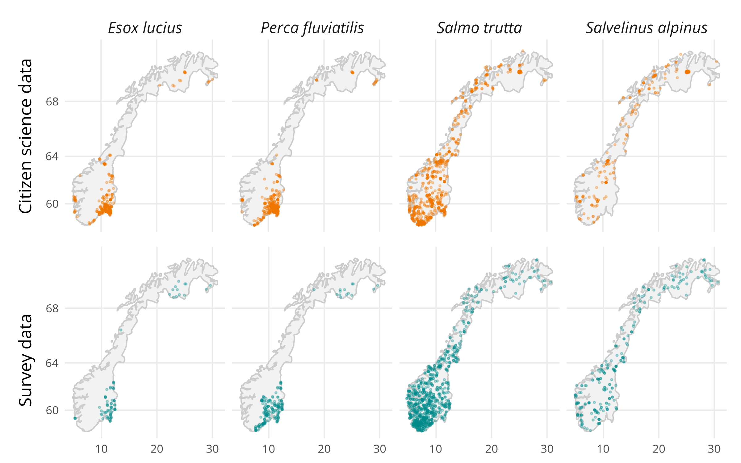
Figure 1: The observed presences of the different fish species in each of the two data sets. Locations are slightly jittered to avoid overplotting.

For the presence/absence survey data, we use a Bernoulli distribution (as described in section 3.2.2), where the presence probability depends on some covariates $x(s)$, along with a spatial field $\xi_{j}(s)$ for species $j\in\{\textit{Salmo trutta, Perca fluviatilis, Esox lucius, Salvelinus alpinus}\}$,

$$Y_{PA,j}(s_{i}) \sim\text{Bernoulli}(p_{PA,j}(s_{i}))$$ (22)

$$\text{cloglog}(p_{PA,j}(s_{i})) =\alpha_{PA,j}+x(s_{i})^{T}\beta_{j}+\xi_{j}(s_{i}).$$ (23)

The presence-only data is fitted with a Poisson point process model (as described in section 3.2.3), where the intensity depends on the same covariates $x(s)$ and the same spatial field $\xi_{j}(s)$, plus an additional spatial field $\xi_{\text{bias}}(s)$ that is unique to the citizen science data, but shared across all fish species:

$$Y_{PO,j}(s_{i}) \sim\text{Poisson}(e^{\eta_{PO,j}(s_{i})})$$ (24)

$$\eta_{PO,j}(s_{i}) =\alpha_{PO,j}+x(s)^{T}\beta_{j}+\xi_{j}(s_{i})+\xi_{\text{bias}}(s_{i}).$$ (25)

In this integrated distribution model, $\xi_{j}(s)$ describes the spatial autocorrelation shared between the datasets. $\xi_{\text{bias}}(s)$ is a bias field that captures the extra spatial variation in the presence-only records, and therefore captures the variation that is likely due to human observation biases rather than the distribution of the fish. The model was fitted using the PointedSDMs (Mostert and O’Hara, 2023a) R package. Code and data for fitting the model, along with a more detailed description, can be found in the Supporting Information at https://github.com/emmaSkarstein/IntegratedLakefish/.

Comparing the observations in the two data sets shown in figure 1, we see that the citizen science data shows certain geographical presences that the survey data does not. That is to be expected, since the survey data is from 1996, and there is reason to believe that the citizen science data shows a more updated view of the species distributions. We present the predictions of the mean log intensity fields for each species from the model in Figure 2.

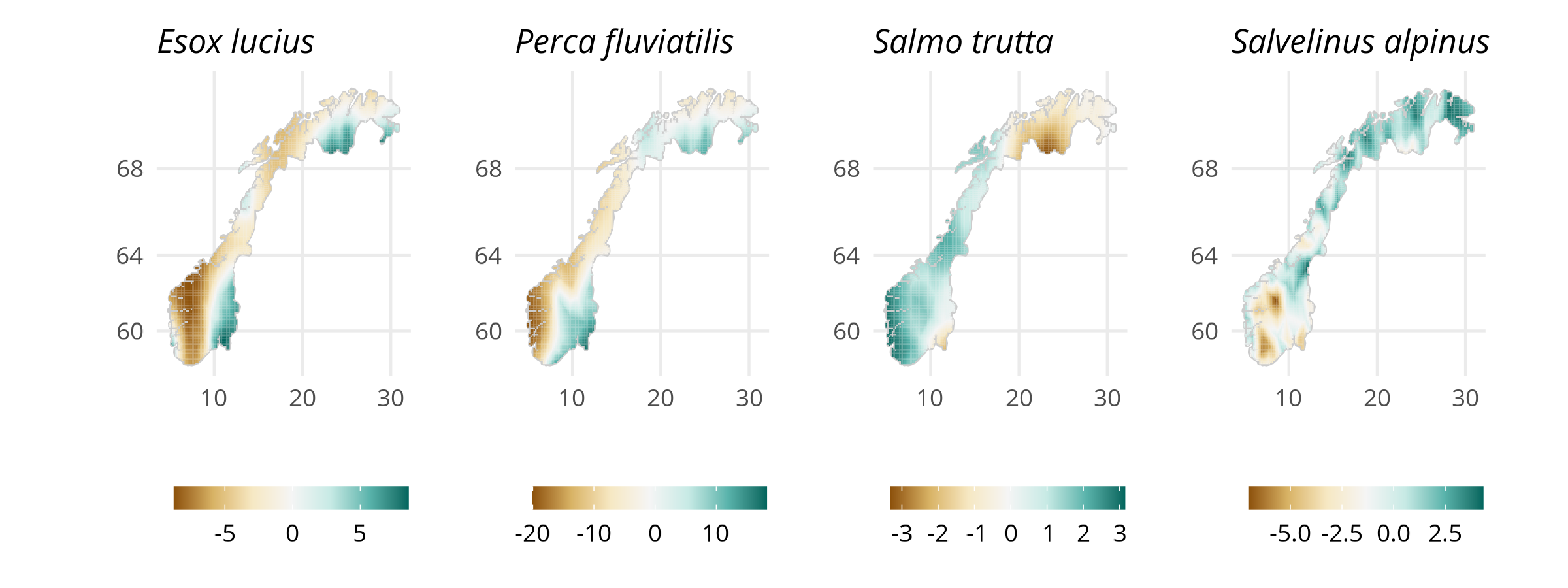
Figure 2: The mean log intensity of the estimated spatial fields for each of the fish species.

5 Discussion

We present a statistical formulation of data integration using a point process framework, including a review of the current literature on data integration, an overview of the data types that are commonly integrated together, and a detailed description of the process model using the point process formulation and various observation models. As an illustration, we have applied the framework to predict the distributions of four fish species in Norwegian lakes, illustrating how this framework allows us to smoothly incorporate information about the observation processes for each of the data sources in a way that respects the data collection, and also makes sense ecologically. In this paper, we focus on the point-process methodology estimated via a joint-likelihood approach, though other methods to construct ISDMs are also possible. Methods such as data pooling and combining independent models may fall within the definition of data integration, but are not recommended for most case scenarios (Fletcher Jr et al., 2019). While other popular methods may be justified, including using an informed prior in a Bayesian setup, using one dataset as a covariate for the other, or by connecting datasets together through a shared covariance matrix, designed to capture patterns present throughout the datasets (Pacifici et al., 2017). Simulation studies comparing the strengths and weaknesses of each of these methods have been completed (Pacifici et al., 2017; Ahmad Suhaimi et al., 2021); they found that the joint-likelihood method worked well when spatial bias in the presence only data was low or statistical components to account the bias were included in the model.

Integrated distribution models fitted with the point process framework has emerged as an ideal approach to utilising the strengths of various data types to estimate state variables in a single analysis better (Dorazio, 2014; Fletcher et al., 2016; Koshkina et al., 2017). Another interesting feature of data integration is the adjustment of the biodiversity biases by using other data types. Data from well designed surveys would be an ideal complement to unstructured data (Koshkina et al., 2017; Fletcher et al., 2016; Pacifici et al., 2017; Giraud et al., 2016). Although data from structured surveys are less numerous, a good design will not be spatially biased, and this can be used to estimate and correct for the bias in the unstructured data (Simmonds et al., 2020). Thus, even in this model-based approach to modelling distributions, a design-based approach will be important if we are to utilise the data that is being collected fully.

Any state variable of interest can be seen as derived quantities of point patterns (Kéry and Royle, 2015). With this, various data types can be integrated together through their basic derived quantity (point patterns) through the point process framework. In contrast to other papers summarised in Table 1 that focus on making inferences and predictions with integrated models, we focused on the statistical properties of the data in the integrated model. Here, we have described the data in terms of its statistical properties, but a more practically useful typology would describe them in terms of the methods used to collect it. Although we may see line transect data and eDNA data both as counts, there are of course large differences in how they are collected, and thus how we should treat them. For example, the correlation between read number (i.e. count) of a sequence in eDNA data and abundance of the species is an area of active research (e.g. Skelton et al., ). A lot of work will therefore be needed to develop specific models for different data sources.

Our framework will only be helpful if it can be implemented in software that can be used by analysts, who may often be ecologists, potentially without formal training in statistics. The approach we have taken is closely linked to models that can be fitted with R-INLA (Rue et al., 2009a) or inlabru Bachl et al. (2019), but for the case study we have used the R-package PointedSDMs (Mostert and O’Hara, 2023a), which builds on inlabru but makes the model fitting a bit more convenient and user friendly. Additionally, the full potential of ISDMs will only be met if we can build a large-scale workflow that designs pipelines to move data from species occurrence databases (notably GBIF) to the modelling framework. An early implementation of such a workflow has been discussed and implemented through the R-package intSDM (Mostert et al., 2022), which has been built to obtain species’ occurrence and environmental data from popular repositories, standardise the data into a coherent framework, and obtain estimates from the model.

We have outlined a framework for integrated distribution models and shown that it can be used for real problems. Within this framework, there is a lot of flexibility, and thus many developments to be explored. One of the key issues is how different datasets may support each other: surveys (for example) will still be important, because they provide reliable data that citizen science data can be calibrated to. But will this mean we should re-evaluate how surveys should be designed? This is the sort of issue that we will have to grapple with if we want to better understand and monitor biodiversity in the future.

Data and code availability

Instructions for accessing the data and code used in the case study are available in the Supporting Information at https://github.com/emmaSkarstein/IntegratedLakefish/. All data is publicly available through GBIF.

References

- A. Lee-Yaw et al. (2022) A. Lee-Yaw, J., L. McCune, J., Pironon, S. and N. Sheth, S. (2022) Species distribution models rarely predict the biology of real populations. Ecography, 2022, e05877.
- Aarts et al. (2012) Aarts, G., Fieberg, J. and Matthiopoulos, J. (2012) Comparative interpretation of count, presence-absence and point methods for species distribution models. Methods in Ecology and Evolution, 3, 177–187. URL: http://doi.wiley.com/10.1111/j.2041-210X.2011.00141.x.
- Aceves-Bueno et al. (2017) Aceves-Bueno, E., Adeleye, A. S., Feraud, M., Huang, Y., Tao, M., Yang, Y. and Anderson, S. E. (2017) The accuracy of citizen science data: a quantitative review. Bulletin of the Ecological Society of America, 98, 278–290.
- Adde et al. (2021) Adde, A., Casabona i Amat, C., Mazerolle, M. J., Darveau, M., Cumming, S. G. and O’Hara, R. B. (2021) Integrated modeling of waterfowl distribution in western canada using aerial survey and citizen science (ebird) data. Ecosphere, 12, e03790.
- Adjei et al. (2023) Adjei, K. P., Sicacha-Parada, J., Steinsland, I. and O’Hara, R. B. (2023) A structural model for the process of collecting biodiversity data. URL: https://www.authorea.com/users/434410/articles/674636-a-structural-model-for-the-process-of-collecting-biodiversity-data.
- Ahmad Suhaimi et al. (2021) Ahmad Suhaimi, S. S., Blair, G. S. and Jarvis, S. G. (2021) Integrated species distribution models: A comparison of approaches under different data quality scenarios. Diversity and Distributions, 27, 1066–1075.
- Anderson (2018) Anderson, C. B. (2018) Biodiversity monitoring, earth observations and the ecology of scale. Ecology letters, 21, 1572–1585.
- Bachl et al. (2019) Bachl, F. E., Lindgren, F., Borchers, D. L. and Illian, J. B. (2019) inlabru: an r package for bayesian spatial modelling from ecological survey data. Methods in Ecology and Evolution, 10, 760–766. URL: https://besjournals.onlinelibrary.wiley.com/doi/abs/10.1111/2041-210X.13168.
- Bird et al. (2014) Bird, T. J., Bates, A. E., Lefcheck, J. S., Hill, N. A., Thomson, R. J., Edgar, G. J., Stuart-Smith, R. D., Wotherspoon, S., Krkosek, M., Stuart-Smith, J. F. et al. (2014) Statistical solutions for error and bias in global citizen science datasets. Biological Conservation, 173, 144–154.
- Blangiardo and Cameletti (2015) Blangiardo, M. and Cameletti, M. (2015) Spatial and spatio-temporal Bayesian models with R-INLA. John Wiley & Sons.
- Boakes et al. (2010) Boakes, E. H., McGowan, P. J., Fuller, R. A., Chang-qing, D., Clark, N. E., O’Connor, K. and Mace, G. M. (2010) Distorted views of biodiversity: spatial and temporal bias in species occurrence data. PLoS biology, 8, e1000385.
- Bowker (2000) Bowker, G. C. (2000) Mapping biodiversity. International Journal of Geographical Information Science, 14, 739–754.
- Bowler et al. (2019) Bowler, D. E., Nilsen, E. B., Bischof, R., O’Hara, R. B., Yu, T. T., Oo, T., Aung, M. and Linnell, J. D. (2019) Integrating data from different survey types for population monitoring of an endangered species: the case of the eld’s deer. Scientific reports, 9, 1–14.
- Bu et al. (2021) Bu, H., McShea, W. J., Wang, D., Wang, F., Chen, Y., Gu, X., Yu, L., Jiang, S., Zhang, F. and Li, S. (2021) Not all forests are alike: the role of commercial forest in the conservation of landscape connectivity for the giant panda. Landscape Ecology, 36, 2549–2564.
- Case and Lawler (2017) Case, M. J. and Lawler, J. J. (2017) Integrating mechanistic and empirical model projections to assess climate impacts on tree species distributions in northwestern north america. Global change biology, 23, 2005–2015.
- Chakraborty et al. (2011) Chakraborty, A., Gelfand, A. E., Wilson, A. M., Latimer, A. M. and Silander, J. A. (2011) Point pattern modelling for degraded presence-only data over large regions. Journal of the Royal Statistical Society: Series C (Applied Statistics), 60, 757–776.
- Chambert et al. (2015) Chambert, T., Miller, D. A. and Nichols, J. D. (2015) Modeling false positive detections in species occurrence data under different study designs. Ecology, 96, 332–339.
- Chevalier et al. (2021) Chevalier, M., Broennimann, O., Cornuault, J. and Guisan, A. (2021) Data integration methods to account for spatial niche truncation effects in regional projections of species distribution. Ecological Applications, 31, e02427.
- Cunningham et al. (2021) Cunningham, C. X., Comte, S., McCallum, H., Hamilton, D. G., Hamede, R., Storfer, A., Hollings, T., Ruiz-Aravena, M., Kerlin, D. H., Brook, B. W. et al. (2021) Quantifying 25 years of disease-caused declines in tasmanian devil populations: host density drives spatial pathogen spread. Ecology Letters, 24, 958–969.
- Cunningham et al. (2022) Cunningham, C. X., Perry, G. L., Bowman, D. M., Forsyth, D. M., Driessen, M. M., Appleby, M., Brook, B. W., Hocking, G., Buettel, J. C., French, B. J. et al. (2022) Dynamics and predicted distribution of an irrupting ‘sleeper’population: fallow deer in tasmania. Biological Invasions, 24, 1131–1147.
- Diggle et al. (2010) Diggle, P. J., Menezes, R. and Su, T.-l. (2010) Geostatistical inference under preferential sampling. Journal of the Royal Statistical Society: Series C (Applied Statistics), 59, 191–232. URL: http://dx.doi.org/10.1111/j.1467-9876.2009.00701.x.
- Donaldson et al. (2016) Donaldson, M. R., Burnett, N. J., Braun, D. C., Suski, C. D., Hinch, S. G., Cooke, S. J. and Kerr, J. T. (2016) Taxonomic bias and international biodiversity conservation research.
- Dorazio (2014) Dorazio, R. M. (2014) Accounting for imperfect detection and survey bias in statistical analysis of presence-only data. Global Ecology and Biogeography, 23, 1472–1484. URL: http://dx.doi.org/10.1111/geb.12216.
- Dormann (2007) Dormann, C. F. (2007) Effects of incorporating spatial autocorrelation into the analysis of species distribution data. Global Ecology and Biogeography, 16, 129–138. URL: http://dx.doi.org/10.1111/j.1466-8238.2006.00279.x.
- Douma et al. (2012) Douma, J. C., Witte, J.-P. M., Aerts, R., Bartholomeus, R. P., Ordoñez, J. C., Venterink, H. O., Wassen, M. J. and Van Bodegom, P. M. (2012) Towards a functional basis for predicting vegetation patterns; incorporating plant traits in habitat distribution models. Ecography, 35, 294–305.
- Duncan et al. (2020) Duncan, S. I., Pynne, J., Parsons, E. I., Fletcher Jr, R. J., Austin, J. D., Castleberry, S. B., Conner, L. M., Gitzen, R. A., Barbour, M. and McCleery, R. A. (2020) Land use and cover effects on an ecosystem engineer. Forest Ecology and Management, 456, 117642.
- Elith et al. (2011) Elith, J., Phillips, S. J., Hastie, T., Dudík, M., Chee, Y. E. and Yates, C. J. (2011) A statistical explanation of MaxEnt for ecologists. Diversity and Distributions, 17, 43–57. URL: http://doi.wiley.com/10.1111/j.1472-4642.2010.00725.x.
- Farley et al. (2018) Farley, S. S., Dawson, A., Goring, S. J. and Williams, J. W. (2018) Situating ecology as a big-data science: Current advances, challenges, and solutions. BioScience, 68, 563–576.
- Farr et al. (2021) Farr, M. T., Green, D. S., Holekamp, K. E. and Zipkin, E. F. (2021) Integrating distance sampling and presence-only data to estimate species abundance. Ecology, 102, e03204.
- Fidino et al. (2022) Fidino, M., Lehrer, E. W., Kay, C. A., Yarmey, N. T., Murray, M. H., Fake, K., Adams, H. C. and Magle, S. B. (2022) Integrated species distribution models reveal spatiotemporal patterns of human–wildlife conflict. Ecological Applications, e2647.
- Fithian et al. (2015) Fithian, W., Elith, J., Hastie, T. and Keith, D. A. (2015) Bias correction in species distribution models: pooling survey and collection data for multiple species. Methods in Ecology and Evolution, 6, 424–438. URL: http://dx.doi.org/10.1111/2041-210X.12242.
- Fithian and Hastie (2012) Fithian, W. and Hastie, T. (2012) Statistical Models for Presence-Only Data: Finite-Sample Equivalence and Addressing Observer Bias. URL: http://arxiv.org/abs/1207.6950.
- Fletcher et al. (2016) Fletcher, R. J., McCleery, R. A., Greene, D. U. and Tye, C. A. (2016) Integrated models that unite local and regional data reveal larger-scale environmental relationships and improve predictions of species distributions. Landscape Ecology, 31, 1369–1382.
- Fletcher Jr et al. (2019) Fletcher Jr, R. J., Hefley, T. J., Robertson, E. P., Zuckerberg, B., McCleery, R. A. and Dorazio, R. M. (2019) A practical guide for combining data to model species distributions. Ecology, 100, e02710.
- Gelfand and Shirota (2019) Gelfand, A. E. and Shirota, S. (2019) Preferential sampling for presence/absence data and for fusion of presence/absence data with presence-only data. Ecological Monographs, 89, e01372.
- Gilbert et al. (2021) Gilbert, N. A., Pease, B. S., Anhalt-Depies, C. M., Clare, J. D., Stenglein, J. L., Townsend, P. A., Van Deelen, T. R. and Zuckerberg, B. (2021) Integrating harvest and camera trap data in species distribution models. Biological Conservation, 258, 109147.
- Giraud et al. (2016) Giraud, C., Calenge, C., Coron, C. and Julliard, R. (2016) Capitalizing on opportunistic data for monitoring relative abundances of species. Biometrics, 72, 649–658.
- Gonzalez et al. (2016) Gonzalez, A., Cardinale, B. J., Allington, G. R., Byrnes, J., Arthur Endsley, K., Brown, D. G., Hooper, D. U., Isbell, F., O’Connor, M. I. and Loreau, M. (2016) Estimating local biodiversity change: a critique of papers claiming no net loss of local diversity. Ecology, 97, 1949–1960.
- Grabow et al. (2022) Grabow, M., Louvrier, J., Planillo, A., Kiefer, S., Drenske, S., Börner, K., Stillfried, M., Hagen, R., Kimmig, S., Straka, T. M. et al. (2022) Data-integration of opportunistic species observations into hierarchical modelling frameworks improves spatial predictions for urban red squirrels. Frontiers in Ecology and Evolution, 735.
- Grattarola et al. (2022) Grattarola, F., Bowler, D. and Keil, P. (2022) Integrating presence-only and presence-absence data to model changes in species geographic ranges: An example of yaguarundí in latin america.
- Guillera-Arroita et al. (2017) Guillera-Arroita, G., Lahoz-Monfort, J. J., van Rooyen, A. R., Weeks, A. R. and Tingley, R. (2017) Dealing with false-positive and false-negative errors about species occurrence at multiple levels. Methods in Ecology and Evolution, 8, 1081–1091.
- Harris et al. (2014) Harris, I., Jones, P., Osborn, T. and Lister, D. (2014) Updated high-resolution grids of monthly climatic observations - the cru ts3.10 dataset. International Journal of Climatology, 34, 623–642. URL: http://dx.doi.org/10.1002/joc.3711.
- Higgins et al. (2012) Higgins, S. I., O’Hara, R. B. and Römermann, C. (2012) A niche for biology in species distribution models. Journal of Biogeography, 39, 2091–2095.
- Hijmans (2012) Hijmans, R. J. (2012) Cross-validation of species distribution models: removing spatial sorting bias and calibration with a null model. Ecology, 93, 679–688. URL: http://dx.doi.org/10.1890/11-0826.1.
- Huberman (2020) Huberman, D. B. (2020) Advances in Spatial Statistics for Ecological and Environmental Data. North Carolina State University.
- Isaac et al. (2020) Isaac, N. J., Jarzyna, M. A., Keil, P., Dambly, L. I., Boersch-Supan, P. H., Browning, E., Freeman, S. N., Golding, N., Guillera-Arroita, G., Henrys, P. A. et al. (2020) Data integration for large-scale models of species distributions. Trends in ecology & evolution, 35, 56–67.
- Isaac et al. (2014) Isaac, N. J., van Strien, A. J., August, T. A., de Zeeuw, M. P. and Roy, D. B. (2014) Statistics for citizen science: extracting signals of change from noisy ecological data. Methods in Ecology and Evolution, 5, 1052–1060.
- Jetz et al. (2012) Jetz, W., McPherson, J. M. and Guralnick, R. P. (2012) Integrating biodiversity distribution knowledge: toward a global map of life. Trends in ecology & evolution, 27, 151–159.
- Kass and Raftery (1995) Kass, R. E. and Raftery, A. E. (1995) Bayes factors. Journal of the American Statistical Association, 90, 773–795. URL: http://www.jstor.org/stable/2291091.
- Keil et al. (2013) Keil, P., Belmaker, J., Wilson, A. M., Unitt, P. and Jetz, W. (2013) Downscaling of species distribution models: a hierarchical approach. Methods in Ecology and Evolution, 4, 82–94. URL: http://dx.doi.org/10.1111/j.2041-210x.2012.00264.x.
- Kelling et al. (2019) Kelling, S., Johnston, A., Bonn, A., Fink, D., Ruiz-Gutierrez, V., Bonney, R., Fernandez, M., Hochachka, W. M., Julliard, R., Kraemer, R. et al. (2019) Using semistructured surveys to improve citizen science data for monitoring biodiversity. BioScience, 69, 170–179.
- Kéry and Royle (2015) Kéry, M. and Royle, J. A. (2015) Applied hierarchical modeling in ecology: Analysis of distribution, abundance and species richness in r and bugs.
- Kéry and Schmid (2004) Kéry, M. and Schmid, H. (2004) Monitoring programs need to take into account imperfect species detectability. Basic and applied ecology, 5, 65–73.
- Koshkina et al. (2017) Koshkina, V., Wang, Y., Gordon, A., Dorazio, R. M., White, M. and Stone, L. (2017) Integrated species distribution models: combining presence-background data and site-occupancy data with imperfect detection. Methods in Ecology and Evolution, 8, 420–430.
- Kosmala et al. (2016) Kosmala, M., Wiggins, A., Swanson, A. and Simmons, B. (2016) Assessing data quality in citizen science. Frontiers in Ecology and the Environment, 14, 551–560.
- Lauret et al. (2022) Lauret, V., Labach, H., Turek, D., Laran, S. and Gimenez, O. (2022) Integrated spatial models foster complementarity between monitoring programmes in producing large-scale bottlenose dolphin indicators. Animal Conservation.
- Liang et al. (2023) Liang, D., Bailey, H., Hoover, A. L., Eckert, S., Zarate, P., Alfaro-Shigueto, J., Mangel, J. C., de Paz Campos, N., Davila, J. Q., Barturen, D. S. et al. (2023) Integrating telemetry and point observations to inform management and conservation of migratory marine species. Ecosphere, 14, e4375.
- Lindgren et al. (2011) Lindgren, F., Rue, H. and Lindström, J. (2011) An explicit link between gaussian fields and gaussian markov random fields: The stochastic partial differential equation approach. Journal of the Royal Statistical Society. Series B: Statistical Methodology, 73, 423–498.
- MacKenzie et al. (2002a) MacKenzie, D. I., Nichols, J. D., Lachman, G. B., Droege, S., Andrew Royle, J. and Langtimm, C. A. (2002a) Estimating site occupancy rates when detection probabilities are less than one. Ecology, 83, 2248–2255.
- MacKenzie et al. (2002b) — (2002b) Estimating site occupancy rates when detection probabilities are less than one. Ecology, 83, 2248–2255. URL: http://dx.doi.org/10.1890/0012-9658(2002)083[2248:ESORWD]2.0.CO;2.
- Mäkinen and Vanhatalo (2018) Mäkinen, J. and Vanhatalo, J. (2018) Hierarchical bayesian model reveals the distributional shifts of arctic marine mammals. Diversity and Distributions, 24, 1381–1394.
- Mandeville et al. (2021) Mandeville, C. P., Koch, W., Nilsen, E. B. and Finstad, A. G. (2021) Open data practices among users of primary biodiversity data. BioScience, 71, 1128–1147.
- Marcantonio et al. (2016) Marcantonio, M., Metz, M., Baldacchino, F., Arnoldi, D., Montarsi, F., Capelli, G., Carlin, S., Neteler, M. and Rizzoli, A. (2016) First assessment of potential distribution and dispersal capacity of the emerging invasive mosquito aedes koreicus in northeast italy. Parasites & vectors, 9, 1–19.
- Marion et al. (2012) Marion, G., McInerny, G. J., Pagel, J., Catterall, S., Cook, A. R., Hartig, F. and O’Hara, R. B. (2012) Parameter and uncertainty estimation for process-oriented population and distribution models: data, statistics and the niche. Journal of Biogeography, 39, 2225–2239.
- Martino et al. (2021) Martino, S., Pace, D. S., Moro, S., Casoli, E., Ventura, D., Frachea, A., Silvestri, M., Arcangeli, A., Giacomini, G., Ardizzone, G. et al. (2021) Integration of presence-only data from several sources: a case study on dolphins’ spatial distribution. Ecography, 44, 1533–1543.
- Matheson (2014) Matheson, C. A. (2014) inaturalist. Reference Reviews.
- McCullagh and Nelder (1989) McCullagh, P. and Nelder, J. (1989) Generalized Linear Models, Second Edition. Chapman & Hall/CRC Monographs on Statistics & Applied Probability. Taylor & Francis. URL: https://books.google.no/books?id=h9kFH2_FfBkC.
- McInerny and Purves (2011) McInerny, G. J. and Purves, D. W. (2011) Fine-scale environmental variation in species distribution modelling: regression dilution, latent variables and neighbourly advice. Methods in Ecology and Evolution, 2, 248–257. URL: http://dx.doi.org/10.1111/j.2041-210X.2010.00077.x.
- Merow et al. (2016) Merow, C., Allen, J. M., Aiello-Lammens, M. and Silander Jr, J. A. (2016) Improving niche and range estimates with maxent and point process models by integrating spatially explicit information. Global Ecology and Biogeography, 25, 1022–1036.
- Merow et al. (2017) Merow, C., Wilson, A. M. and Jetz, W. (2017) Integrating occurrence data and expert maps for improved species range predictions. Global Ecology and Biogeography, 26, 243–258. URL: http://dx.doi.org/10.1111/geb.12539.
- Miller et al. (2011) Miller, D. A., Nichols, J. D., McClintock, B. T., Grant, E. H. C., Bailey, L. L. and Weir, L. A. (2011) Improving occupancy estimation when two types of observational error occur: Non-detection and species misidentification. Ecology, 92, 1422–1428.
- Miller et al. (2019) Miller, D. A., Pacifici, K., Sanderlin, J. S. and Reich, B. J. (2019) The recent past and promising future for data integration methods to estimate species’ distributions. Methods in Ecology and Evolution, 10, 22–37.
- Møller et al. (1998) Møller, J., Syversveen, A. R. and Waagepetersen, R. P. (1998) Log gaussian cox processes. Scandinavian journal of statistics, 25, 451–482.