Two Higgs doublet model fitting and $t\bar{t}b\bar{b}$ signal at the ILC

Abstract

One of the most straightforward extensions of the standard model (SM) is having an additional Higgs doublet to the SM, namely the two Higgs doublet models(THDM). In the type-I model, an additional Higgs doublet is introduced that does not couple to any fermion via the Yukawa interaction. Considering various theoretical and phenomenological constraints, we have found the best-fitted parameter set in the type-I model using the minimum $\chi^{2}$ method by scanning the model’s parameter space. We show that this optimal parameter set can be probed by precisely analyzing the decay processes $D^{+}\rightarrow\mu^{+}\nu_{\mu}$, $B^{0}\rightarrow K^{*}\mu^{+}\mu^{-}$. Moreover, the decay channels $h\rightarrow s\bar{s}$, $W^{+}W^{-}$ and $gg$ can be used to distinguish the model from the SM. For a direct search of the model at future colliders, we have proposed an investigation of the $e^{+}e^{-}\rightarrow t\bar{t}b\bar{b}$ process at the ILC to detect the new physics of the model. Considering the initial state radiation correction and applying appropriate background cuts, the calculation result of the scattering cross section shows that it is feasible to observe a clear and unique signal in the $t\bar{b}$ invariant mass distribution corresponding to the charged Higgs pair creations.

1 Introduction

In the standard model (SM), the minimal one that can generate the fermion masses after the spontaneous symmetry breaking, the scalar sector consists of only one Higgs doublet. Since scalars are so flexible for model building, they have been used in various new physics models to address theoretical challenges and experimental anomalies. Although the SM-like Higgs boson was discovered at the LHC, there may be still more Higgs bosons in nature that come from an extended scalar sector. Among various extensions of the SM, the two Higgs doublet model (THDM)[1] is an important one since its structure can be found in many new physics models such as the minimal supersymmetric extension of the SM [2, 3, 4], grand unified theories[5, 6], composite Higgs models, axion models[7, 8]. Moreover, the additional CP violation from the scalar potential of the THDM helps realize the successful electroweak baryogenesis[9, 10, 11, 12, 13, 14, 15, 16].

The THDM generally suffers from the flavour-changing neutral current (FCNC) problem. The two Yukawa coupling matrices relevant to the Higgs doublets in the model can not be diagonalized simultaneously by the rotational matrices relating the initial fermion states and their mass eigenstates, unlike the situation in the SM. This leads to the dangerous tree-level FCNCs that are strictly constrained by experiments. To ameliorate this problem, a $Z_{2}$ symmetry was introduced in the theory[17] so that a given fermion couples to only one Higgs doublet, as dictated by the theorem of Glashow and Weinberg [18]. Another way to avoid the FCNCs is to assume the flavour alignment of the Yukawa couplings. According to that, the Yukawa matrices of the two scalar doublets are proportional[19, 20, 21]. The free parameter space of the THDM has been investigated, taking into account various constraints, including the LEP and LHC data, flavour observables and theoretical requirements[22, 23, 24, 25, 26, 27, 28, 29, 30, 31, 32, 33, 34, 35, 36, 37, 38, 39, 40, 41, 42, 43, 44, 45, 46, 47, 48, 49, 50, 51, 52, 53, 54, 55] The global fit to the THDM with the soft $Z_{2}$-symmetry breaking was performed in Refs. [56, 57, 58]. For the case of the aligned THDM, the global fit was carried out in Refs. [59, 60]. It has been shown that searches for the THDM signatures in future colliders are promising [61, 62, 63, 64, 65, 66, 67, 68, 69].

In this paper, we focus our analysis on the THDM of type I, where the fermions only couple to one scalar doublet, while the other does not couple to any fermion. Therefore, all of the fermion masses are generated by the vacuum expectation value of that scalar doublet. We perform the data fitting of the model to various theoretical and phenomenological constraints, taking into account the results of the LEP, the Tevatron, and the LHC experiments, the measurements of flavour observables, and the current world-average value of the $W$-boson mass. Using the best-fit point, we then examine the four-fermion-production channel $e^{+}e^{-}\rightarrow t\,\bar{t}\,b\,\bar{b}$ and investigate the possibility of detecting the new physics signals at the International Linear Collider (ILC).

The structure of the paper is as follows. In Section 2, we briefly review the type-I THDM. In Section 3, the data fitting is performed to find the best-fit point of the model. The $e^{+}e^{-}$ scattering analysis is performed in Section 4 to look for possible signals of the model at the ILC. Finally, Section 5 is devoted to summary and discussion.

2 Two Higgs doublet model

In the THDM, two scalar doublets are introduced to generate masses for fermions and gauge bosons after acquiring their vacuum expectation values. Its Lagrangian is given by

$$\mathcal{L}_{\text{THDM}} =\mathcal{L}_{\text{SM}}^{\text{no scalar}}+\mathcal{L}_{\text{scalar}}+\mathcal{L}_{\text{Yukawa}},$$ (1)

where $\mathcal{L}_{\text{SM}}^{\text{no scalar}}$ involves the SM terms without any scalar particles, $\mathcal{L}_{\text{scalar}}$ is the Lagrangian for the two scalar doublets including their kinetic terms with covariant derivatives and the scalar potential $\mathcal{V}_{\text{scalar}}$, and $\mathcal{L}_{\text{Yukawa}}$ is the one describing the Yukawa interactions between fermions and scalars. To avoid the dangerous FCNCs emerging from the Yukawa Lagrangian, a $Z_{2}$ symmetry is usually imposed in the theory. Under this discrete symmetry, the two scalars transform differently, i.e. one is even ($\Phi_{1}\rightarrow\Phi_{1}$) while the other is odd ($\Phi_{2}\rightarrow-\Phi_{2}$) by convention. Therefore, for any choice of $Z_{2}$-transformation rules for the fermions that keeps $\mathcal{L}_{\text{Yukawa}}$ invariant [70], a given fermion can couple to only one scalar field:

$$\mathcal{L}_{\text{Yukawa}} =-\bar{Q}_{L}Y_{u}\tilde{\Phi}_{u}u_{R}-\bar{Q}_{L}Y_{d}\Phi_{d}d_{R}-\bar{L}_{L}Y_{\ell}\Phi_{\ell}\ell_{R}+\text{h.c.},$$ (2)

where $\Phi_{u,d,\ell}$ is either $\Phi_{1}$ or $\Phi_{2}$. Depending on the $Z_{2}$ charges of the fermions, the THDM are categorized into four distinct types, so-called I, II, X, and Y. For example, in the type-I THDM, the left(right)-handed fermions are $Z_{2}$ even (odd). Hence, the scalar doublet $\Phi_{2}$ couples to all of the fermions and generates their mases after the spontaneous breaking of the electroweak symmetry, while $\Phi_{1}$ does not (namely, $\Phi_{u}=\Phi_{d}=\Phi_{\ell}=\Phi_{2}$ in Eq. (2)).

For the scalar potential of $\Phi_{1}$ and $\Phi_{2}$, we allow the soft $Z_{2}$ breaking term so that the discrete symmetry can be restored in the UV limit [71]. The scalar potential is given by

$$V(\Phi_{1},\Phi_{2}) =m_{11}^{2}\Phi_{1}^{\dagger}\Phi_{1}+m_{22}^{2}\Phi_{2}^{\dagger}\Phi_{2}-\left(m_{12}^{2}\Phi_{1}^{\dagger}\Phi_{2}+\text{h.c.}\right)$$

$$+\frac{\lambda_{1}}{2}(\Phi_{1}^{\dagger}\Phi_{1})^{2}+\frac{\lambda_{2}}{2}(\Phi_{2}^{\dagger}\Phi_{2})^{2}+\lambda_{3}(\Phi_{1}^{\dagger}\Phi_{1})(\Phi_{2}^{\dagger}\Phi_{2})+\lambda_{4}|\Phi_{1}^{\dagger}\Phi_{2}|^{2}+\left(\frac{\lambda_{5}}{2}(\Phi_{1}^{\dagger}\Phi_{2})^{2}+\text{h.c.}\right).$$ (3)

Denoting the vacuum expectation values (VEVs) of the neutral components of the two scalar doublets as $\langle\Phi_{1,2}^{0}\rangle={v_{1,2}}/{\sqrt{2}}$, the minimization equations, ${\partial V}/{\partial\Phi^{0}_{i}}|_{\Phi^{0}_{i}=\langle\Phi_{i}^{0}\rangle}=0$, of the scalar potential allow us to represent $m_{11}^{2}$ and $m_{22}^{2}$ in terms of other parameters [72, 73]:

$$m_{11}^{2} =m_{12}^{2}\frac{v_{2}}{v_{1}}-\frac{\lambda_{1}}{2}v_{1}^{2}-\frac{1}{2}(\lambda_{3}+\lambda_{4}+\lambda_{5})v_{2}^{2},$$ (4)

$$m_{22}^{2} =m_{12}^{2}\frac{v_{1}}{v_{2}}-\frac{\lambda_{1}}{2}v_{1}^{2}-\frac{1}{2}(\lambda_{3}+\lambda_{4}+\lambda_{5})v_{2}^{2}.$$ (5)

It is convenient to work in the Higgs basis $(\phi,\phi^{\prime})$ where only one of them ($\phi$) acquires a nonzero VEV, $\langle\phi^{0}\rangle=\frac{v}{\sqrt{2}}$, where $v=\sqrt{v_{1}^{2}+v_{2}^{2}}$. The transformation between the two bases reads

$$\left(\begin{matrix}\Phi_{1}\\ \Phi_{2}\end{matrix}\right) =\left(\begin{matrix}\cos\beta&-\sin\beta\\ \sin\beta&\cos\beta\end{matrix}\right)\left(\begin{matrix}\phi\\ \phi^{\prime}\end{matrix}\right),$$ (6)

where $\tan\beta={v_{2}}/{v_{1}}$. The components of the scalar doublets, $\phi$ and $\phi^{\prime}$, are

$$\phi=\left(\begin{matrix}G^{+}\\ \frac{h_{1}^{\prime}+v+iG^{0}}{\sqrt{2}}\end{matrix}\right),\quad\phi^{\prime}=\left(\begin{matrix}H^{+}\\ \frac{h_{2}^{\prime}+iA}{\sqrt{2}}\end{matrix}\right),$$ (7)

where $(H^{\pm},G^{\pm})$ and $(A,G^{0})$ are the mass eigenstates. In the Higgs basis, the massive components ($H^{\pm}$ and $A$) are identified as the charged Higgs boson and the CP-odd Higgs, while the massless components ($G^{\pm}$ and $G^{0}$) are the are the Nambu-Goldstone bosons to be absorbed by the $W^{\pm}$ and $Z$ gauge bosons. The mass eigenstates of the CP-even Higgs are obtained by another rotation:

$$\left(\begin{matrix}h^{\prime}_{1}\\ h^{\prime}_{2}\end{matrix}\right) =\left(\begin{matrix}\cos(\beta-\alpha)&\sin(\beta-\alpha)\\ -\sin(\beta-\alpha)&\cos(\beta-\alpha)\end{matrix}\right)\left(\begin{matrix}H\\ h\end{matrix}\right).$$ (8)

Hereafter, we utilize abbreviations $s_{\bullet}:=\sin\bullet$ and $c_{\bullet}:=\cos\bullet$. The masses of the physical states ($m_{h,H,A,H^{\pm}}$) and the mixing angles ($\alpha$, $\beta$) are related to the couplings $\lambda_{1,...,5}$ in the scalar potential as [72, 74]

$$\lambda_{1} =\frac{1}{v^{2}c^{2}_{\beta}}\left(c^{2}_{\alpha}m_{H}^{2}+s^{2}_{\alpha}m_{h}^{2}-m_{12}^{2}\frac{s_{\beta}}{c_{\beta}}\right),$$ (9)

$$\lambda_{2} =\frac{1}{v^{2}s^{2}_{\beta}}\left(s^{2}_{\alpha}m_{H}^{2}+c^{2}_{\alpha}m_{h}^{2}-m_{12}^{2}\frac{c_{\beta}}{s_{\beta}}\right),$$ (10)

$$\lambda_{3} =\frac{2m_{H^{\pm}}^{2}}{v^{2}}+\frac{s_{2\alpha}}{v^{2}s_{2\beta}}(m_{H}^{2}-m_{h}^{2})-\frac{m_{12}^{2}}{v^{2}s_{\beta}c_{\beta}},$$ (11)

$$\lambda_{4} =\frac{m_{A}^{2}-2m_{H^{\pm}}^{2}}{v^{2}}+\frac{m_{12}^{2}}{v^{2}s_{\beta}c_{\beta}},$$ (12)

$$\lambda_{5} =\frac{m_{12}^{2}}{v^{2}s_{\beta}c_{\beta}}-\frac{m_{A}^{2}}{v^{2}}.$$ (13)

Identifying $h$ as the SM-like Higgs boson with $m_{h}=125.25$ GeV [75], and the SM VEV $v=(\sqrt{2}G_{F})^{1/2}\approx 246$ GeV, where $G_{F}$ is the Fermi constant, the scalar potential is then determined by six independent real parameters:

$$m_{H},\,m_{A},\,m_{H^{\pm}},\,m_{12}^{2},\,\tan\beta,\,\sin(\beta-\alpha).$$ (14)

3 Parameter optimization

We consider the theoretical constraints, including the scalar potential’s stability, the S-matrix’s tree-level unitarity[76], and the perturbativity The phenomenological constraints are those on the oblique parameters ($S$, $T$, $U$) and the various flavour observables related to the decay of $B$ and $D$ mesons. Furthermore, we consider the constraint given by the world-averaging value of the $W$ boson mass the Particle Data Group[75]. For this purpose, the theoretically predicted value for $m_{W}$ in the THDM with the loop contributions is given as [77]

$$m_{W} =\sqrt{\left(m_{W}^{\text{SM}}\right)^{2}+\frac{\alpha\cos^{2}{\theta_{W}}}{\cos^{2}{\theta_{W}}-\sin^{2}{\theta_{W}}}m_{Z}^{2}\left(-\frac{1}{2}S+\cos^{2}{\theta_{W}}T+\frac{\cos^{2}{\theta_{W}}-\sin^{2}{\theta_{W}}}{4\sin^{2}{\theta_{W}}}U\right)}\,,$$ (15)

where $m_{W}^{\text{SM}}$, $\theta_{W}$and $\alpha$ are the SM predicted value for the $W$ boson mass, the Weinberg mixing angle and the fine structure constant, respectively. The experimental data for these constraints are given in Table 1.

For the numerical analysis, we use the 2HDMC package version 1.8.0 [78] to examine the theoretical constraints, to calculate the oblique parameters, the braching ratios and decay widths of the Higgs bosons. The flavor observables are calculated by the SuperIso package version 4.1 [79, 80, 81]. The HiggsBounds package version 5.10.2 [82, 83, 84, 85, 86, 87] is used to check if a parameter point of the model is consistent with the Higgs searches at the LEP, the Tevatron and the LHC.

Observables	Exp. data	[Refs.]
S	$-0.02\pm 0.10$	[75]
T	$0.03\pm 0.12$	[75]
U	$0.01\pm 0.11$	[75]
BR($b\rightarrow s\gamma$)	$(3.49\pm 0.19)\times 10^{-4}$	[88]
BR($B_{s}^{0}\rightarrow\mu^{+}\mu^{-}$)	$(2.95\pm 0.41)\times 10^{-9}$	[88]
BR($B_{d}^{0}\rightarrow\mu^{+}\mu^{-}$)	$(0.12\pm 0.08)\times 10^{-9}$	[89]
BR($B_{u}^{+}\rightarrow\tau^{+}\nu_{\tau}$)	$(1.09\pm 0.24)\times 10^{-4}$	[75]
BR($D_{s}^{+}\rightarrow\tau^{+}\nu_{\tau}$)	$(5.32\pm 0.11)\times 10^{-2}$	[75]
BR($D_{s}^{+}\rightarrow\mu^{+}\nu_{\mu}$)	$(5.43\pm 0.15)\times 10^{-3}$	[75]
BR($D^{+}\rightarrow\mu^{+}\nu_{\mu}$)	$(3.74\pm 0.17)\times 10^{-4}$	[75]
BR($B^{+}\rightarrow\bar{D}^{0}\tau^{+}\nu_{\tau}$)	$(7.7\pm 2.5)\times 10^{-3}$	[75]
$\dfrac{\text{BR}(B\rightarrow D\tau\nu_{\tau})}{\text{BR}(B\rightarrow D\ell\nu_{\ell})}$	$0.339\pm 0.030$	[88]
BR$(\bar{B}\rightarrow X_{s}\ell^{+}\ell^{-})_{\text{low}}$	$(1.58\pm 0.37)\times 10^{-6}$	[90, 91]
BR$(\bar{B}\rightarrow X_{s}\ell^{+}\ell^{-})_{\text{high}}$	$(4.8\pm 1.0)\times 10^{-7}$	[90, 91]
BR$(B^{0}\rightarrow K^{*}\mu^{+}\mu^{-})_{\text{low}}$	$(1.68\pm 0.15)\times 10^{-7}$	[92]
BR$(B^{0}\rightarrow K^{*}\mu^{+}\mu^{-})_{\text{high}}$	$(1.74\pm 0.14)\times 10^{-7}$	[92]
$m_{W}$ (GeV)	$80.377\pm 0.012$	[75]

Table 1: List of observables and experimental data used in the fitting.

The ranges of the independent input parameters are chosen as follows

$$0.01 <\tan\beta<100,$$ (16)

$$125\text{ GeV} <m_{H},m_{A},m_{H^{\pm}}<2000\text{ GeV},$$ (17)

$$0 <\sin(\beta-\alpha)<1,$$ (18)

$$-10^{8}\text{ GeV}^{2} <m_{12}^{2}<10^{8}\text{ GeV}^{2}.$$ (19)

For each parameter point, we determine the value of the $\chi^{2}$ function defined as follows

$$\chi^{2}_{\text{Total}} =\chi^{2}_{\text{HS}}+\sum_{n}\chi^{2}_{n},$$ (20)

where $\chi^{2}_{\text{HS}}$ is calculated by HiggsSignals package version 2.6.2 [93, 94, 95, 96], and the sum in the second term is taken over all the considered observables in Table 1. The best fit point is the one minimizing the above $\chi^{2}$ function.

To achieve this goal, we randomly scan over the parameter space with the MultiNest package version 3.11[97, 98, 99], where the nested sampling algorithm is used. An optimum parameter point minimizing the $\chi^{2}$ function in Eq. (20) is obtained after the convergence criterion is satisfied. This scan is carried out many times to avoid falling into some local minimum. Subsequently, the smallest minimum found in the above steps is refined further using the Nelder-Mead simplex algorithm [100, 101] with a high precision. As a result, we obtained the best-fit parameter set shown in Table 2.

Parameter	best-fit value
$\tan\beta$	66.87117763
$m_{H}$	530.3595712 GeV
$m_{A}$	536.2373210 GeV
$m_{H^{\pm}}$	493.9314561 GeV
$\sin(\beta-\alpha)$	0.9999735699
$m_{12}^{2}$	4.206078567 $\times 10^{3}$ GeV2

Table 2: The best-fit parameter set.

Observables	Theor. prediction	Pulls ($\sigma$)
S	3.83$\times 10^{-3}$	$0.24$
T	2.74$\times 10^{-2}$	$-0.021$
U	9.58$\times 10^{-5}$	$-0.090$
BR($b\rightarrow s\gamma$)	3.18 $\times 10^{-4}$	$-1.64$
BR($B_{s}^{0}\rightarrow\mu^{+}\mu^{-}$)	2.96$\times 10^{-9}$	$0.022$
BR($B_{d}^{0}\rightarrow\mu^{+}\mu^{-}$)	9.45$\times 10^{-11}$	$-0.32$
BR($B_{u}^{+}\rightarrow\tau^{+}\nu_{\tau}$)	8.37$\times 10^{-5}$	$-1.05$
BR($D_{s}^{+}\rightarrow\tau^{+}\nu_{\tau}$)	5.12$\times 10^{-2}$	$-1.79$
BR($D_{s}^{+}\rightarrow\mu^{+}\nu_{\mu}$)	5.26$\times 10^{-3}$	$-1.15$
BR($D^{+}\rightarrow\mu^{+}\nu_{\mu}$)	4.14$\times 10^{-4}$	$2.37$
BR($B^{+}\rightarrow\bar{D}^{0}\tau^{+}\nu_{\tau}$)	6.77$\times 10^{-3}$	$-0.37$
$\dfrac{\text{BR}(B\rightarrow D\tau\nu_{\tau})}{\text{BR}(B\rightarrow D\ell\nu_{\ell})}$	0.315	$-0.81$
BR$(\bar{B}\rightarrow X_{s}\ell^{+}\ell^{-})_{\text{low}}$	1.41$\times 10^{-6}$	$-0.45$
BR$(\bar{B}\rightarrow X_{s}\ell^{+}\ell^{-})_{\text{high}}$	4.12$\times 10^{-7}$	$-0.68$
BR$(B^{0}\rightarrow K^{*}\mu^{+}\mu^{-})_{\text{low}}$	2.09$\times 10^{-7}$	$2.70$
BR$(B^{0}\rightarrow K^{*}\mu^{+}\mu^{-})_{\text{high}}$	1.98$\times 10^{-7}$	$1.73$
$m_{W}$ (GeV)	80.356	$-1.75$

Table 3: The theoretical predictions in the THDM and pulls of physical observables for the best-fit point with $m_{h}=125.25$ GeV [75].

In Table 3, the theoretical values of the observables listed in Table 1 are presented for the case of the best-fit point. The pulls in terms of the standard deviation for each observable are indicated in the last column of this table. We observe that the pulls for other observables are all smaller than $2\sigma$, except for the pulls corresponding to the branching ratios of the decay processes $D^{+}\rightarrow\mu^{+}\nu_{\mu}$ and $B^{0}\rightarrow K^{*}\mu^{+}\mu^{-}$ at low momentum transfer, that are 2.37 and 2.70 respectively. Therefore, these two decay processes will be the sensitive probes to test the best-fit point in the future when the experimental precision is increased.

Observables	THDM	SM	$\delta(\%)$	Exp. data	Dev. $(\sigma)$
BR($h\rightarrow s\bar{s}$)	2.239$\times 10^{-4}$	2.445$\times 10^{-4}$	$-$8.4
BR($h\rightarrow c\bar{c}$)	2.750$\times 10^{-2}$	2.872$\times 10^{-2}$	$-$4.3
BR($h\rightarrow b\bar{b}$)	6.127$\times 10^{-1}$	5.784$\times 10^{-1}$	5.9	$(5.3\pm 0.8)\times 10^{-1}$	1.03
BR($h\rightarrow\mu\bar{\mu}$)	2.099$\times 10^{-4}$	2.162$\times 10^{-4}$	$-$2.9	$(2.6\pm 1.3)\times 10^{-4}$	$-$0.39
BR($h\rightarrow\tau\bar{\tau}$)	5.928$\times 10^{-2}$	6.232$\times 10^{-2}$	$-$4.9	$(6.0^{+0.8}_{-0.7})\times 10^{-2}$	$-$0.10
BR($h\rightarrow\gamma\gamma$)	2.150$\times 10^{-3}$	2.270$\times 10^{-3}$	$-$5.3	$(2.50\pm 0.20)\times 10^{-3}$	$-$1.75
BR($h\rightarrow ZZ$)	2.488$\times 10^{-2}$	2.680$\times 10^{-2}$	$-$7.2	$(2.80\pm 0.30)\times 10^{-2}$	$-$1.04
BR($h\rightarrow W^{+}W^{-}$)	1.984$\times 10^{-1}$	2.178$\times 10^{-1}$	$-$8.9	$(2.57\pm 0.25)\times 10^{-1}$	$-$2.34
BR($h\rightarrow Z\gamma$)	1.457$\times 10^{-3}$	1.554$\times 10^{-3}$	$-$6.2	$(3.2\pm 1.5)\times 10^{-3}$	$-$1.16
BR($h\rightarrow gg$)	7.327$\times 10^{-2}$	8.168$\times 10^{-2}$	$-$10.3
$\Gamma^{h}_{\text{total}}$ (GeV)	4.373$\times 10^{-3}$	4.122$\times 10^{-3}$	6.1	$(3.2^{+2.4}_{-1.7})\times 10^{-3}$	0.49

Table 4: The branching ratios and the total decay width of the light Higgs boson ($m_{h}=125.25$ GeV [75]) for the best-fit point (2nd column) in the THDM in comparison with the SM predictions[102, 103] (3rd column), and the experimental data [75] (5th column). The 4th column ($\delta$) shows the relative differences between the THDM values and the SM predictions. The 6th column indicates the deviations between the THDM values and the experimental data.

The properties of the SM-like Higgs boson like the branching ratios and the total decay width have been calculated for the best-fit point of the THDM. The results are shown in the second column of Table 4 in comparison with the SM predicted values [102, 103] in the third column. The relative differences between the branching ratios and the total width predicted by these two models are presented in the fourth column. We see that the most significant relative differences come from the branching fractions of the decay channels of the light Higgs boson to $gg$, $W^{+}W^{-}$, and $s\bar{s}$ that are $-$10.3%, $-$8.9%, and $-$8.4, respectively. Therefore, these channels can effectively distinguish the two models once the high-precision measurements are carried out in the future. The current experimental data of the branching ratios and the total width are shown in the fifth column of Table 4. The deviations in terms of $\sigma$ of the corresponding THDM predictions from the data are presented in the sixth column. The most significant deviation is $-2.34\sigma$ corresponding to the decay process $h\rightarrow W^{+}W^{-}$. Hence, this channel will be the most sensitive probe to test the viability of the THDM best-fit point in the future.

4 $e^{+}e^{-}\rightarrow t\bar{t}b\bar{b}$ channel at the ILC

In this section, we investigate the possibility to probe the best-fit point of the type-I THDM at the ILC via the $t\bar{t}b\bar{b}$ channel. This task has been performed using the combination of two packages, Sarah version 4.15.5 and Grace version 2.2.1.7.

4.1 Calculation methods

Sarah [104, 105, 106] is a software package written in Mathematica to investigate any models of particle physics with broken or unbroken gauge symmetries. This tool automatically generates all possible Feynman rules for the considered model. With the inputs of the particle content as representations of the gauge symmetry and the model’s Lagrangian, the outputs of the model are written by Sarah in the style of the CalcHEP/ComHEP[107, 108, 109] model files.

The Grace system is a set of programs for automatically calculating scattering amplitudes in quantum field theory developed at KEK. The user can obtain numerical results of various cross-sections and decay widths by selecting the appropriate phase space option. The public version of Grace can perform calculations in the SM and the minimal supersymmetric standard model [110, 111]. This system can be extended by adding particles and interactions to a few text files describing the model-dependent part as appropriate. For example, an extension to the THDM and analysis using it was done in Refs.[63, 112].

Processes		Number of diagrams	Agreement
Initial	Final
$\tau^{+}\tau^{-}$	$b\bar{b}$	6	$+5.30\times 10^{-14}$
$\tau^{+}\tau^{-}$	$t\bar{t}Z$	36	$+6.66\times 10^{-16}$
$\nu_{\mu}\mu^{+}$	$ZW^{+}$	5	$-1.88\times 10^{-15}$
$t\bar{t}$	$w^{+}h^{0}$	5	$+8.88\times 10^{-16}$
$t\bar{t}$	$b\bar{b}$	6	$0.00$
$t\bar{t}$	$h^{0}h^{0}$	6	$0.00$
$t\bar{t}$	$h^{0}h^{0}h^{0}$	88	$0.00$
$t\bar{t}$	$u\bar{u}$	6	$0.00$
$t\bar{t}$	$W^{+}W^{-}$	7	$0.00$
$t\bar{t}$	$Zh^{0}$	5	$+3.10\times 10^{-15}$
$t\bar{t}$	$Zh^{0}h^{0}$	63	$+2.88\times 10^{-15}$
$t\bar{t}$	$ZZ$	4	$0.00$
$t\bar{t}$	$h^{0}ZZ$	43	$+1.77\times 10^{-15}$
$t\bar{t}$	$ZZZ$	36	$-5.55\times 10^{-16}$
$u\bar{d}$	$h^{0}w^{+}$	5	$0.00$
$u\bar{d}$	$W^{+}ZZ$	43	$-4.99\times 10^{-15}$
$c\bar{c}$	$W^{+}W^{-}$	7	$0.00$
$W^{+}W^{-}$	$\gamma\gamma$	9	$0.00$
$W^{+}W^{-}$	$\gamma h^{0}$	7	$-1.33\times 10^{-15}$
$W^{+}W^{-}$	$h^{0}h^{0}$	9	$+3.08\times 10^{-14}$
$W^{+}W^{-}$	$\gamma h^{0}h^{0}$	93	$+9.83\times 10^{-12}$
$W^{+}W^{-}$	$W^{+}W^{-}$	9	$0.00$
$W^{+}W^{-}$	$Zh^{0}$	7	$-1.55\times 10^{-15}$
$W^{+}W^{-}$	$Zh^{0}h^{0}$	117	$-2.72\times 10^{-14}$
$W^{+}W^{-}$	$ZZ$	9	$0.00$
$ZZ$	$h^{0}h^{0}$	9	$+1.55\times 10^{-14}$
$ZZ$	$ZZ$	6	$0.00$

Table 5: Test for the gauge invariance

Here, we extended Grace utilizing Sarah described above to perform calculations. The Grace system has mainly two databases for generating programs to evaluate scattering amplitudes: a database of all particles and interaction vertices appearing in the model and a database of computer programs for numerical evaluations of a given scattering process. The former is a list of particles with their quantum numbers, e.g., spin, parity, mass, representation in the gauge groups, etc. All interaction vertices with corresponding interaction types are listed in the model file. The latter is a set of computer programs to numerically evaluate spinor and vector wave functions, particle propagators with the gauge fixing parameter, interaction vertices, etc. When the initial and final particles, as well as the interaction order (a power of coupling constants), are specified, Grace generates all possible Feynman diagrams based on the covariant gauge, including Goldstone bosons and then produces a set of computer programs to evaluate the scattering amplitude based on the generated diagrams numerically. The amplitude is numerically integrated using an adaptive Monte Carlo method. The Grace system also has a program database, namely the kinematics, to assign particle momenta from independent random numbers. The Grace system keeps redundancy owing to the gauge parameters; thus, we can test generated programs if they give amplitudes independent from values of the gauge parameters.

In this study, we have generated a database of particles and interactions of the type-I THDM using Sarah. We convert outputs created by Sarah to adapt with the Grace system using a Mathematica code. The created database is numerically checked owing to the gauge-parameter independence of the system. We have prepared 27 scattering processes concerning the fermions, the gauge bosons and the Higgs bosons covering all particles and vertices in our target process. We compare the numerical results with two gauge choices: the Feynman gauge and the unitary gauge. We obtain consistent results within the numerical precision of 64-bit floating number (binary64) format as summarized in Table 5.

4.2 Possible signals at the ILC

This section discusses the discovery potential for the experimental signals of the type-I THDM with the best-fit parameters at the future linear electron-positron collider, such as the ILC. The ILC is a linear electron-positron collider, operating at 250 to 500 GeV center-of-mass (CM) energies with high luminosity, which may be extended to 1 TeV or more in the upgrade stage. It is based on 1.3 GHz superconducting radio-frequency (SCRF) accelerating technology [113, 114]. The ILC is proposed to be constructed in the Kitakami Mountains in Tohoku, Japan. It is an international project running for more than 20 years, collaborated by more than 300 institutes, universities, and laboratories. The primary physics aim of the ILC is to determine the future direction of particle physics via the precise measurements of the couplings of the Higgs boson with other elementary particles. This facility can also study a wide variety of elementary-particle physics and nuclear physics.

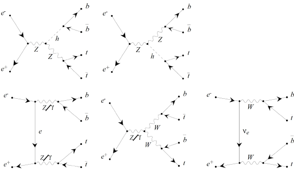
Figure 1: Diagrams of the SM background. The first row shows backgrounds involving the SM Higgs, while the second row shows non-Higgs backgrounds.

The prediction of the extra Higgs bosons, in addition to the standard one, is the prominent feature of the THDM. For the experimental target, we chose the process $e^{+}e^{-}\rightarrow b\bar{b}t\bar{t}$ since the Yukawa couplings of Higgs bosons are proportional to the fermion masses, given that the $t$ and $b$ quarks are the heaviest and the second heaviest fermions, respectively. Therefore, we can expect a sizable cross section for this process. This process includes pair creations of all possible Higgs bosons, such as the CP-even, CP-odd and charged Higgs particles. Among the signal and background sub-diagrams of the target process, the light Higgs productions associated with the $Z$ boson and the gauge-boson pair-creation processes, depicted in Figure 1, mainly contribute to the total cross section. We identify the light (CP-even) Higgs boson in the THDM to the experimentally observed Higgs boson by the LHC experiments; thus, the light-Higgs production process is the background in the search for the THDM signal. In our calculation, we apply the simple condition $m^{~{}}_{b\bar{b}}>50$ GeV to reduce the background due to the photo-productions of the $b$-quark pair. The main part of the SM background due to the $h$ and $Z$ resonances can be eliminated by vetoing the $b$-quark pair creations that fulfill the conditions:

$$|M_{b\bar{b}}-m_{Z}|<10~{}\text{GeV},~{}~{}\text{and}~{}~{}|M_{b\bar{b}}-m_{h}|<10~{}\text{GeV}.$$ (21)

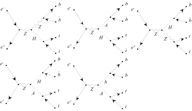
Figure 2: Diagrams of signal processes involving the neutral Higgs bosons in the THDM.

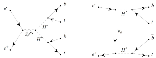
Figure 3: Diagrams of signal processes involving the charged Higgs bosons in to the THDM.

The first category of the signal processes is the pair creation of the heavy neutral Higgs bosons and the single Higgs boson production associated with a Z boson, depicted in Figure 2. The second category of the THDM signal processes consists of the charged Higgs boson pair creations depicted in Figure 3. We can identify the signal processes mentioned above by looking for the resonances of $t\bar{t}$ , $b\bar{b}$ , $t\bar{b}$ and $b\bar{t}$ pairs. All the Higgs bosons have very narrow decay widths. Therefore, we expect the experimental signal of quark-pair invariant mass to be relatively clear after being smeared due to the detector effect. The Feynman diagrams in Figures 1-3 are not all the diagrams contributing to the cross section. We have calculated the cross sections utilizing all possible Feynman diagrams (516 diagrams in total), including Goldstone bosons. In the following calculations, we use the standard model parameters listed in Table 6 and the best-fit parameters of the THDM in Table 2. We have calculated cross sections at the tree level using the Grace system. The typical contributions of the higher order correction is about $\mathcal{O}(10\%)$ for the electroweak processes at the ILC energies. It is known that the initial state photon radiation (ISR) gives the most significant contribution to the total cross sections.

SM parameter	input value
$m^{~{}}_{Z}$	91.1876 GeV
$m^{~{}}_{W}$	80.377 GeV
$m^{~{}}_{h}$	125.25 GeV
$\alpha(m^{~{}}_{Z})$	1/128.07
$\sin^{2}{\theta_{W}}$	$1-{m_{W}^{2}}/{m_{Z}^{2}}$

Table 6: The SM parameters[75] used in calculations.

The effect of the ISR can be factorized when the total energy of the emitted photons is sufficiently small compared to the beam energy. The calculations under such an approximation are called the “soft photon approximation (SPA)”. Using the SPA, the corrected cross sections with the ISR, denoted by $\sigma^{~{}}_{\text{ISR}}$, can be obtained from the tree-level cross sections $\sigma^{~{}}_{\text{Tree}}$ using a structure function $H(x,s)$ as follows:

$$\sigma^{~{}}_{\text{ISR}} =\int^{1}_{0}dx\,H(x,s)\,\sigma^{~{}}_{\text{Tree}}\left(s(1-x)\right),$$ (22)

where $s$ is the CM energy squared and $x$ is the energy fraction of an emitted photon.

The structure function is provided using the perturbative method with the SPA. The radiator function $D(x,s)$, which corresponds to the square root of the structure function, gives the probability of an electron with energy $\sqrt{s}/2$ emitting a photon with an energy fraction $x$. In this method, electrons and positrons can emit unbalanced energies; thus, a finite boost of the CM system is realized, which is more realistic than using the structure function. The radiator function is given as[115]

$$D(1-x,s)^{2} =H(x,s)=\Delta_{2}\beta x^{\beta-1}-\Delta_{1}\beta\left(1-\frac{x}{2}\right)$$

$$+\frac{\beta^{2}}{8}\left[-4(2-x)\log{x}-\frac{1+3(1-x)^{2}}{x}\log{(1-x)}-2x\right],$$ (23)

where

$$\beta =\frac{2\alpha}{\pi}\left(\log{\frac{s}{m_{e}^{2}}}-1\right),\quad~{}~{}\Delta_{1}=1+\delta_{1},~{}~{}\Delta_{2}=1+\delta_{1}+\delta_{2},$$

$$\delta_{1} =\frac{\alpha}{\pi}\left(\frac{3}{2}L+\frac{\pi^{2}}{3}-2\right),~{}~{}~{}~{}\delta_{2}=\left(\frac{\alpha L}{\pi}\right)^{2}\left(-\frac{1}{18}L+\frac{119}{72}-\frac{\pi^{2}}{3}\right),$$

and

$$L =\ln\frac{s}{m_{e}^{2}}.$$

This result was obtained based on the perturbative calculations for initial-state photon emission diagrams up to the two-loop order [115]. The terms proportional to $\alpha^{2}$ in Eq.(23) correspond to the two-loop diagrams. The ISR corrected cross section is provided using the radiator function as

$$\sigma^{~{}}_{\text{ISR}} =\int^{1}_{0}dx\int^{1}_{0}dy\hskip 1.00006ptD(x,s)D(y,s)\,\sigma^{~{}}_{\text{Tree}}\left(sxy\right).$$ (24)

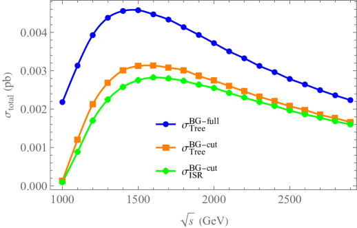
Figure 4: The $e^{+}e^{-}\rightarrow b\bar{b}t\bar{t}$ total cross section as a function of $\sqrt{s}$ at the ILC energies and beyond. The blue (orange) line shows the total cross section without (with) the background cut (21). The realistic cross section including the ISR correction is shown by the green line.

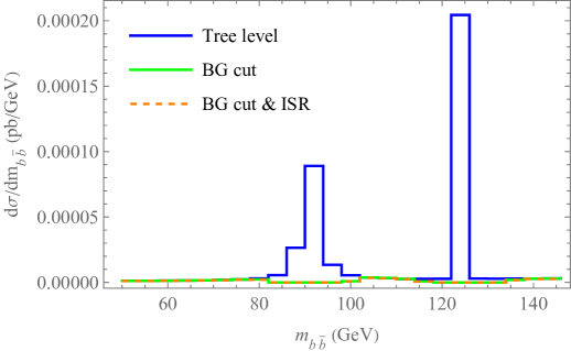
Figure 5: The $b\bar{b}$-invariant mass distributions without and with the background cut (21) and the ISR correction for the case $\sqrt{s}=1500$ GeV. The background cut vetos events from the $Z$-boson the light-Higgs decays. The ISR effect is very small to be seen in the figure, leading to the overlap between the orange and the green lines.

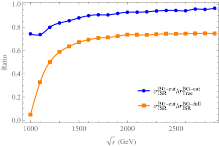
Figure 6: The reduction ratio of cross sections with the background cut and the ISR correction.

We obtain the total cross sections of the target process as shown in Figure 4. The total cross section increases from $\sqrt{s}\simeq 1000$ GeV owing to the charged-Higgs pair-creation threshold, peaks around 1500 GeV, and then gradually decreases according to the increase in the CM energy. Among all diagrams of the target process, the SM-like Higgs production associated with the Z boson gives the most significant background, as shown in Figure 5. The figure shows the clear twin peaks of the $b$-quark pair invariant mass at the $Z$-boson and the light-Higgs masses. After cutting the events satisfying (21) around the $Z$ and Higgs masses, the charged Higgs pair production cross section is dominated, while other Higgs contributions (the heavy and CP-odd Higgs) are negligibly small. The cuts (21) eliminate about $30\%$ of the total events in high energy region as shown by the orange line in Figure 6, which is consistent to the SM background cross section. The ISR correction leads to the effective CM energy smaller than the nominal energy due to the lost in term of radiation; thus, the signal cross sections are decreasing about $10$ to $20$% of the total cross sections after applying this correction, also shown by the blue line in Figure 6.

The charged Higgs signal is obvious in the $t\bar{b}$ ($b\bar{t}$) invariant mass distribution, as shown in Figure 7. The signal peak is significant even before the background cut because the SM does not have any structure on the $t\bar{b}$ invariant mass distribution, and the phase space contribution in this energy region is very small. The ISR affects the mass distribution only $10$% effect; thus, we can expect a clear signal of the charged Higgs production after the smearing due to the detector effects.

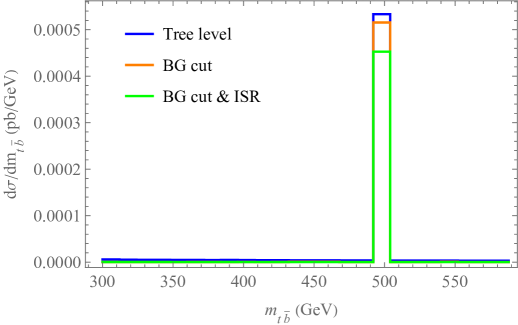
Figure 7: The $t\bar{b}\,(b\bar{t})$-invariant mass distributions without and with the background cut and the ISR correction for the case $\sqrt{s}=1500$ GeV. The background cut does not significantly reduce the number of signal events.

On the other hand, the $t$-quark pair invariant mass does not have any structure, as shown in Figure 8. When the heavy CP-even and CP-odd Higgs production, depicted in Figure 2, have significant cross sections, we can observe peak(s) on this distribution. However, the THDM with the best-fit parameter set gives a small differential cross section with respect to $m_{t\bar{t}}$. Thus, it is very challenging to experimentally observe the signal via the $m_{t\bar{t}}$ distribution.

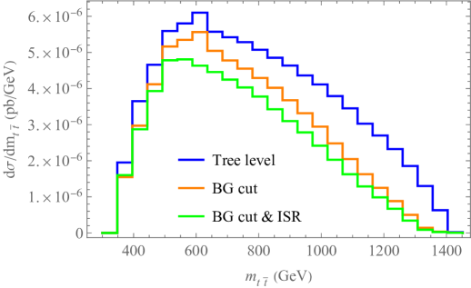
Figure 8: The $t\bar{t}$-invariant mass distributions without and with the background cut and the ISR correction for the case $\sqrt{s}=1500$ GeV.

After the experimental cuts and the ISR correction, the total cross sections are greater than $1$fb for the CM energy greater than 1100 GeV. Therefore, if we assume $10$ ab^-1 of an integrated luminosity at the ILC, we can expect $\mathcal{O}(10^{4})$ almost-background-free signal events. Even if we assume several per cent of the reconstruction efficiency of the $t$ and $b$ quarks, we can easily distinguish the THDM signal from the SM background.

5 Summary

We have investigated the phenomenology of the type-I THDM, an extension of the SM adding one more Higgs doublet that does not couple directly to fermions via the Yukawa interaction. The Lagrangian satisfies the $Z_{2}$ symmetry except for the softly breaking term in the scalar potential. We took into account various theoretical and phenomenological constraints such as the perturbativity, unitarity, stability, oblique parameters, the Higgs searches by high-energy experiments (LEP, Tevatron and LHC ), the world-average $W$-boson mass, as well as the flavour physics observables. We found the best-fit point to the measured observables by performing a systematic scan over the space of independent parameters. The pulls for the branching ratios of the decays $D^{+}\rightarrow\mu^{+}\nu_{\mu}$, $B^{0}\rightarrow K^{*}\mu^{+}\mu^{-}$ at low momentum transfer are noticeable. Therefore, they are suitable probes to test the viability of the best-fit point by more precise measurements of these channels in the future. The branching ratios of the SM-like Higgs boson decaying to $s\bar{s}$, $W^{+}W^{-}$ and $gg$ show non-negligible deviations compared to the SM predictions. The results urge careful and precise analyses of these light-Higgs decay channels at the LHC and future colliders.

Considering the possibility of observing the THDM new physics at one of the most promising future colliders, the ILC, we have proposed the analysis of the best-fit point using the $e^{+}e^{-}\rightarrow t\bar{t}b\bar{b}$ scattering process. We have utilized the Grace system to calculate the total cross-sections and the invariant mass distributions. Since the standard Grace system does not have a model file of the THDM, we have prepared it automatically using the Sarah system. We have tested the consistency of the created model file utilizing the gauge-parameter independence of the scattering amplitudes for various scattering processes. We have considered the ISR effect in the calculation, which is known to contribute most to the total cross-sections at the one-loop level. Consequently, we clarified that the THDM with the best-fit parameter set can be probed by observing the clear charged Higgs signal on the $t\bar{b}$ invariant mass distribution. On the other hand, the signals of other Higgs bosons included in the THDM, the heavy CP-even Higgs boson and the CP-odd Higgs boson, are hardly observed at the ILC since they do not provide significant cross sections. The reasons are that the best-fit point predicts the light Higgs boson consistent with observations to date, leading to the small couplings of other heavy neutral Higgs bosons to the fermions. Meanwhile, the couplings of charged Higgs to the heavy fermions are of $\mathcal{O}(1)$.

References

- [1] H.E. Haber, G.L. Kane and T. Sterling, The Fermion Mass Scale and Possible Effects of Higgs Bosons on Experimental Observables, Nucl. Phys. B 161 (1979) 493.
- [2] S.P. Martin, A Supersymmetry primer, Adv. Ser. Direct. High Energy Phys. 18 (1998) 1 [hep-ph/9709356].
- [3] N. Okada and H.M. Tran, Discrimination of Supersymmetric Grand Unified Models in Gaugino Mediation, Phys. Rev. D 83 (2011) 053001 [1011.1668].
- [4] H.M. Tran, T. Kon and Y. Kurihara, Discrimination of SUSY breaking models using single-photon processes at future e+e- linear colliders, Mod. Phys. Lett. A 26 (2011) 949 [1012.1730].
- [5] D. Croon, T.E. Gonzalo, L. Graf, N. Košnik and G. White, GUT Physics in the era of the LHC, Front. in Phys. 7 (2019) 76 [1903.04977].
- [6] T. Fukuyama, N. Okada and H.M. Tran, Alternative renormalizable (10) GUTs and data fitting, Nucl. Phys. B 954 (2020) 114992 [1907.02948].
- [7] R.D. Peccei and H.R. Quinn, CP Conservation in the Presence of Instantons, Phys. Rev. Lett. 38 (1977) 1440.
- [8] R.D. Peccei and H.R. Quinn, Constraints Imposed by CP Conservation in the Presence of Instantons, Phys. Rev. D 16 (1977) 1791.
- [9] N. Turok and J. Zadrozny, Dynamical generation of baryons at the electroweak transition, Phys. Rev. Lett. 65 (1990) 2331.
- [10] A.E. Nelson, D.B. Kaplan and A.G. Cohen, Why there is something rather than nothing: Matter from weak interactions, Nucl. Phys. B 373 (1992) 453.
- [11] K. Funakubo, A. Kakuto and K. Takenaga, The Effective potential of electroweak theory with two massless Higgs doublets at finite temperature, Prog. Theor. Phys. 91 (1994) 341 [hep-ph/9310267].
- [12] J.M. Cline, K. Kainulainen and A.P. Vischer, Dynamics of two Higgs doublet CP violation and baryogenesis at the electroweak phase transition, Phys. Rev. D 54 (1996) 2451 [hep-ph/9506284].
- [13] J.M. Cline and P.-A. Lemieux, Electroweak phase transition in two Higgs doublet models, Phys. Rev. D 55 (1997) 3873 [hep-ph/9609240].
- [14] M. Laine and K. Rummukainen, Two Higgs doublet dynamics at the electroweak phase transition: A Nonperturbative study, Nucl. Phys. B 597 (2001) 23 [hep-lat/0009025].
- [15] L. Fromme, S.J. Huber and M. Seniuch, Baryogenesis in the two-Higgs doublet model, JHEP 11 (2006) 038 [hep-ph/0605242].
- [16] A.T. Davies, C.D. froggatt, G. Jenkins and R.G. Moorhouse, Baryogenesis constraints on two Higgs doublet models, Phys. Lett. B 336 (1994) 464.
- [17] G.C. Branco, P.M. Ferreira, L. Lavoura, M.N. Rebelo, M. Sher and J.P. Silva, Theory and phenomenology of two-Higgs-doublet models, Phys. Rept. 516 (2012) 1 [1106.0034].
- [18] S.L. Glashow and S. Weinberg, Natural Conservation Laws for Neutral Currents, Phys. Rev. D 15 (1977) 1958.
- [19] A.V. Manohar and M.B. Wise, Flavor changing neutral currents, an extended scalar sector, and the Higgs production rate at the CERN LHC, Phys. Rev. D 74 (2006) 035009 [hep-ph/0606172].
- [20] A. Pich and P. Tuzon, Yukawa Alignment in the Two-Higgs-Doublet Model, Phys. Rev. D 80 (2009) 091702 [0908.1554].
- [21] A. Peñuelas and A. Pich, Flavour alignment in multi-Higgs-doublet models, JHEP 12 (2017) 084 [1710.02040].
- [22] M. Jung, A. Pich and P. Tuzon, Charged-Higgs phenomenology in the Aligned two-Higgs-doublet model, JHEP 11 (2010) 003 [1006.0470].
- [23] C.-Y. Chen and S. Dawson, Exploring Two Higgs Doublet Models Through Higgs Production, Phys. Rev. D 87 (2013) 055016 [1301.0309].
- [24] A. Celis, V. Ilisie and A. Pich, LHC constraints on two-Higgs doublet models, JHEP 07 (2013) 053 [1302.4022].
- [25] C.-W. Chiang and K. Yagyu, Implications of Higgs boson search data on the two-Higgs doublet models with a softly broken symmetry, JHEP 07 (2013) 160 [1303.0168].
- [26] B. Grinstein and P. Uttayarat, Carving Out Parameter Space in Type-II Two Higgs Doublets Model, JHEP 06 (2013) 094 [1304.0028].
- [27] O. Eberhardt, U. Nierste and M. Wiebusch, Status of the two-Higgs-doublet model of type II, JHEP 07 (2013) 118 [1305.1649].
- [28] A. Celis, V. Ilisie and A. Pich, Towards a general analysis of LHC data within two-Higgs-doublet models, JHEP 12 (2013) 095 [1310.7941].
- [29] S. Chang, S.K. Kang, J.-P. Lee, K.Y. Lee, S.C. Park and J. Song, Two Higgs doublet models for the LHC Higgs boson data at 7 and 8 TeV, JHEP 09 (2014) 101 [1310.3374].
- [30] L. Wang and X.-F. Han, Status of the aligned two-Higgs-doublet model confronted with the Higgs data, JHEP 04 (2014) 128 [1312.4759].
- [31] J. Baglio, O. Eberhardt, U. Nierste and M. Wiebusch, Benchmarks for Higgs Pair Production and Heavy Higgs boson Searches in the Two-Higgs-Doublet Model of Type II, Phys. Rev. D 90 (2014) 015008 [1403.1264].
- [32] V. Ilisie and A. Pich, Low-mass fermiophobic charged Higgs phenomenology in two-Higgs-doublet models, JHEP 09 (2014) 089 [1405.6639].
- [33] S. Kanemura, K. Tsumura, K. Yagyu and H. Yokoya, Fingerprinting nonminimal Higgs sectors, Phys. Rev. D 90 (2014) 075001 [1406.3294].
- [34] J. Bernon, J.F. Gunion, Y. Jiang and S. Kraml, Light Higgs bosons in Two-Higgs-Doublet Models, Phys. Rev. D 91 (2015) 075019 [1412.3385].
- [35] N. Craig, F. D’Eramo, P. Draper, S. Thomas and H. Zhang, The Hunt for the Rest of the Higgs Bosons, JHEP 06 (2015) 137 [1504.04630].
- [36] G. Abbas, A. Celis, X.-Q. Li, J. Lu and A. Pich, Flavour-changing top decays in the aligned two-Higgs-doublet model, JHEP 06 (2015) 005 [1503.06423].
- [37] F.J. Botella, G.C. Branco, M. Nebot and M.N. Rebelo, Flavour Changing Higgs Couplings in a Class of Two Higgs Doublet Models, Eur. Phys. J. C 76 (2016) 161 [1508.05101].
- [38] A. Ilnicka, M. Krawczyk and T. Robens, Inert Doublet Model in light of LHC Run I and astrophysical data, Phys. Rev. D 93 (2016) 055026 [1508.01671].
- [39] J. Bernon, J.F. Gunion, H.E. Haber, Y. Jiang and S. Kraml, Scrutinizing the alignment limit in two-Higgs-doublet models: mh=125 GeV, Phys. Rev. D 92 (2015) 075004 [1507.00933].
- [40] J. Bernon, J.F. Gunion, H.E. Haber, Y. Jiang and S. Kraml, Scrutinizing the alignment limit in two-Higgs-doublet models. II. mH=125 GeV, Phys. Rev. D 93 (2016) 035027 [1511.03682].
- [41] V. Cacchio, D. Chowdhury, O. Eberhardt and C.W. Murphy, Next-to-leading order unitarity fits in Two-Higgs-Doublet models with soft breaking, JHEP 11 (2016) 026 [1609.01290].
- [42] H. Bélusca-Maïto, A. Falkowski, D. Fontes, J.C. Romão and J.a.P. Silva, Higgs EFT for 2HDM and beyond, Eur. Phys. J. C 77 (2017) 176 [1611.01112].
- [43] A. Ilnicka, T. Robens and T. Stefaniak, Constraining Extended Scalar Sectors at the LHC and beyond, Mod. Phys. Lett. A 33 (2018) 1830007 [1803.03594].
- [44] D. Dercks and T. Robens, Constraining the Inert Doublet Model using Vector Boson Fusion, Eur. Phys. J. C 79 (2019) 924 [1812.07913].
- [45] F.J. Botella, F. Cornet-Gomez and M. Nebot, Flavor conservation in two-Higgs-doublet models, Phys. Rev. D 98 (2018) 035046 [1803.08521].
- [46] P. Sanyal, Limits on the Charged Higgs Parameters in the Two Higgs Doublet Model using CMS TeV Results, Eur. Phys. J. C 79 (2019) 913 [1906.02520].
- [47] J. Herrero-Garcia, M. Nebot, F. Rajec, M. White and A.G. Williams, Higgs Quark Flavor Violation: Simplified Models and Status of General Two-Higgs-Doublet Model, JHEP 02 (2020) 147 [1907.05900].
- [48] S. Karmakar and S. Rakshit, Relaxed constraints on the heavy scalar masses in 2HDM, Phys. Rev. D 100 (2019) 055016 [1901.11361].
- [49] N. Chen, T. Han, S. Li, S. Su, W. Su and Y. Wu, Type-I 2HDM under the Higgs and Electroweak Precision Measurements, JHEP 08 (2020) 131 [1912.01431].
- [50] F. Arco, S. Heinemeyer and M.J. Herrero, Exploring sizable triple Higgs couplings in the 2HDM, Eur. Phys. J. C 80 (2020) 884 [2005.10576].
- [51] M. Aiko, S. Kanemura, M. Kikuchi, K. Mawatari, K. Sakurai and K. Yagyu, Probing extended Higgs sectors by the synergy between direct searches at the LHC and precision tests at future lepton colliders, Nucl. Phys. B 966 (2021) 115375 [2010.15057].
- [52] F.J. Botella, F. Cornet-Gomez and M. Nebot, Electron and muon anomalies in general flavour conserving two Higgs doublets models, Phys. Rev. D 102 (2020) 035023 [2006.01934].
- [53] P. Athron, C. Balazs, T.E. Gonzalo, D. Jacob, F. Mahmoudi and C. Sierra, Likelihood analysis of the flavour anomalies and g – 2 in the general two Higgs doublet model, JHEP 01 (2022) 037 [2111.10464].
- [54] F.J. Botella, F. Cornet-Gomez, C. Miró and M. Nebot, Muon and electron anomalies in a flavor conserving 2HDM with an oblique view on the CDF value, Eur. Phys. J. C 82 (2022) 915 [2205.01115].
- [55] F.J. Botella, F. Cornet-Gomez, C. Miró and M. Nebot, New Physics hints from scalar interactions and , 2302.05471.
- [56] D. Chowdhury and O. Eberhardt, Global fits of the two-loop renormalized Two-Higgs-Doublet model with soft Z2 breaking, JHEP 11 (2015) 052 [1503.08216].
- [57] D. Chowdhury and O. Eberhardt, Update of Global Two-Higgs-Doublet Model Fits, JHEP 05 (2018) 161 [1711.02095].
- [58] J. Haller, A. Hoecker, R. Kogler, K. Mönig, T. Peiffer and J. Stelzer, Update of the global electroweak fit and constraints on two-Higgs-doublet models, Eur. Phys. J. C 78 (2018) 675 [1803.01853].
- [59] O. Eberhardt, A.P. Martínez and A. Pich, Global fits in the Aligned Two-Higgs-Doublet model, JHEP 05 (2021) 005 [2012.09200].
- [60] A. Karan, V. Miralles and A. Pich, Updated global fit of the ATHDM with heavy scalars, 2307.15419.
- [61] F. Kling, H. Li, A. Pyarelal, H. Song and S. Su, Exotic Higgs Decays in Type-II 2HDMs at the LHC and Future 100 TeV Hadron Colliders, JHEP 06 (2019) 031 [1812.01633].
- [62] A. Adhikary, S. Banerjee, R. Kumar Barman and B. Bhattacherjee, Resonant heavy Higgs searches at the HL-LHC, JHEP 09 (2019) 068 [1812.05640].
- [63] T. Kon, T. Nagura, T. Ueda and K. Yagyu, Double Higgs boson production at colliders in the two-Higgs-doublet model, Phys. Rev. D 99 (2019) 095027 [1812.09843].
- [64] F. Arco, S. Heinemeyer and M.J. Herrero, Sensitivity to triple Higgs couplings via di-Higgs production in the 2HDM at colliders, Eur. Phys. J. C 81 (2021) 913 [2106.11105].
- [65] T. Han, S. Li, S. Su, W. Su and Y. Wu, Heavy Higgs bosons in 2HDM at a muon collider, Phys. Rev. D 104 (2021) 055029 [2102.08386].
- [66] S. Li, H. Song and S. Su, Probing Exotic Charged Higgs Decays in the Type-II 2HDM through Top Rich Signal at a Future 100 TeV pp Collider, JHEP 11 (2020) 105 [2005.00576].
- [67] Y.-B. Liu and S. Moretti, Probing the top-Higgs boson FCNC couplings via the channel at the HE-LHC and FCC-hh, Phys. Rev. D 101 (2020) 075029 [2002.05311].
- [68] Y.-L. Chung, K. Cheung and S.-C. Hsu, Sensitivity of two-Higgs-doublet models on Higgs-pair production via bb¯bb¯ final state, Phys. Rev. D 106 (2022) 095015 [2207.09602].
- [69] H. Bahl, P. Bechtle, S. Heinemeyer, S. Liebler, T. Stefaniak and G. Weiglein, HL-LHC and ILC sensitivities in the hunt for heavy Higgs bosons, Eur. Phys. J. C 80 (2020) 916 [2005.14536].
- [70] M. Aoki, S. Kanemura, K. Tsumura and K. Yagyu, Models of Yukawa interaction in the two Higgs doublet model, and their collider phenomenology, Phys. Rev. D 80 (2009) 015017 [0902.4665].
- [71] I.F. Ginzburg and M. Krawczyk, Symmetries of two Higgs doublet model and CP violation, Phys. Rev. D 72 (2005) 115013 [hep-ph/0408011].
- [72] A. Barroso, P.M. Ferreira, I.P. Ivanov and R. Santos, Metastability bounds on the two Higgs doublet model, JHEP 06 (2013) 045 [1303.5098].
- [73] M. Aoki, T. Komatsu and H. Shibuya, Possibility of a multi-step electroweak phase transition in the two-Higgs doublet models, PTEP 2022 (2022) 063B05 [2106.03439].
- [74] I. Chakraborty and A. Kundu, Scalar potential of two-Higgs doublet models, Phys. Rev. D 92 (2015) 095023 [1508.00702].
- [75] Particle Data Group collaboration, Review of Particle Physics, PTEP 2022 (2022) 083C01.
- [76] I.F. Ginzburg and I.P. Ivanov, Tree-level unitarity constraints in the most general 2HDM, Phys. Rev. D 72 (2005) 115010 [hep-ph/0508020].
- [77] M.E. Peskin and T. Takeuchi, Estimation of oblique electroweak corrections, Phys. Rev. D 46 (1992) 381.
- [78] D. Eriksson, J. Rathsman and O. Stal, 2HDMC: Two-Higgs-Doublet Model Calculator Physics and Manual, Comput. Phys. Commun. 181 (2010) 189 [0902.0851].
- [79] F. Mahmoudi, SuperIso: A Program for calculating the isospin asymmetry of B — K* gamma in the MSSM, Comput. Phys. Commun. 178 (2008) 745 [0710.2067].
- [80] F. Mahmoudi, SuperIso v2.3: A Program for calculating flavor physics observables in Supersymmetry, Comput. Phys. Commun. 180 (2009) 1579 [0808.3144].
- [81] F. Mahmoudi, SuperIso v3.0, flavor physics observables calculations: Extension to NMSSM, Comput. Phys. Commun. 180 (2009) 1718.
- [82] P. Bechtle, O. Brein, S. Heinemeyer, G. Weiglein and K.E. Williams, HiggsBounds: Confronting Arbitrary Higgs Sectors with Exclusion Bounds from LEP and the Tevatron, Comput. Phys. Commun. 181 (2010) 138 [0811.4169].
- [83] P. Bechtle, O. Brein, S. Heinemeyer, G. Weiglein and K.E. Williams, HiggsBounds 2.0.0: Confronting Neutral and Charged Higgs Sector Predictions with Exclusion Bounds from LEP and the Tevatron, Comput. Phys. Commun. 182 (2011) 2605 [1102.1898].
- [84] P. Bechtle, O. Brein, S. Heinemeyer, O. Stal, T. Stefaniak, G. Weiglein et al., Recent Developments in HiggsBounds and a Preview of HiggsSignals, PoS CHARGED2012 (2012) 024 [1301.2345].
- [85] P. Bechtle, O. Brein, S. Heinemeyer, O. Stål, T. Stefaniak, G. Weiglein et al., : Improved Tests of Extended Higgs Sectors against Exclusion Bounds from LEP, the Tevatron and the LHC, Eur. Phys. J. C 74 (2014) 2693 [1311.0055].
- [86] P. Bechtle, D. Dercks, S. Heinemeyer, T. Klingl, T. Stefaniak, G. Weiglein et al., HiggsBounds-5: Testing Higgs Sectors in the LHC 13 TeV Era, Eur. Phys. J. C 80 (2020) 1211 [2006.06007].
- [87] H. Bahl, V.M. Lozano, T. Stefaniak and J. Wittbrodt, Testing exotic scalars with HiggsBounds, Eur. Phys. J. C 82 (2022) 584 [2109.10366].
- [88] Heavy Flavor Averaging Group, HFLAV collaboration, Averages of b-hadron, c-hadron, and -lepton properties as of 2021, Phys. Rev. D 107 (2023) 052008 [2206.07501].
- [89] LHCb collaboration, Analysis of Neutral B-Meson Decays into Two Muons, Phys. Rev. Lett. 128 (2022) 041801 [2108.09284].
- [90] T. Huber, T. Hurth and E. Lunghi, Inclusive : complete angular analysis and a thorough study of collinear photons, JHEP 06 (2015) 176 [1503.04849].
- [91] Belle-II collaboration, The Belle II Physics Book, PTEP 2019 (2019) 123C01 [1808.10567].
- [92] LHCb collaboration, Measurements of the S-wave fraction in decays and the differential branching fraction, JHEP 11 (2016) 047 [1606.04731].
- [93] P. Bechtle, S. Heinemeyer, O. Stål, T. Stefaniak and G. Weiglein, : Confronting arbitrary Higgs sectors with measurements at the Tevatron and the LHC, Eur. Phys. J. C 74 (2014) 2711 [1305.1933].
- [94] O. Stål and T. Stefaniak, Constraining extended Higgs sectors with HiggsSignals, PoS EPS-HEP2013 (2013) 314 [1310.4039].
- [95] P. Bechtle, S. Heinemeyer, O. Stål, T. Stefaniak and G. Weiglein, Probing the Standard Model with Higgs signal rates from the Tevatron, the LHC and a future ILC, JHEP 11 (2014) 039 [1403.1582].
- [96] P. Bechtle, S. Heinemeyer, T. Klingl, T. Stefaniak, G. Weiglein and J. Wittbrodt, HiggsSignals-2: Probing new physics with precision Higgs measurements in the LHC 13 TeV era, Eur. Phys. J. C 81 (2021) 145 [2012.09197].
- [97] F. Feroz and M.P. Hobson, Multimodal nested sampling: an efficient and robust alternative to MCMC methods for astronomical data analysis, Mon. Not. Roy. Astron. Soc. 384 (2008) 449 [0704.3704].
- [98] F. Feroz, M.P. Hobson and M. Bridges, MultiNest: an efficient and robust Bayesian inference tool for cosmology and particle physics, Mon. Not. Roy. Astron. Soc. 398 (2009) 1601 [0809.3437].
- [99] F. Feroz, M.P. Hobson, E. Cameron and A.N. Pettitt, Importance Nested Sampling and the MultiNest Algorithm, Open J. Astrophys. 2 (2019) 10 [1306.2144].
- [100] J.A. Nelder and R. Mead, A Simplex Method for Function Minimization, Comput. J. 7 (1965) 308.
- [101] R. O’Neill, Algorithm as 47: Function minimization using a simplex procedure, Journal of the Royal Statistical Society. Series C (Applied Statistics) 20 (1971) 338.
- [102] LHC Higgs Cross Section Working Group collaboration, Handbook of LHC Higgs Cross Sections: 4. Deciphering the Nature of the Higgs Sector, 1610.07922.
- [103] LHC Higgs Cross Section Working Group collaboration, Handbook of LHC Higgs Cross Sections: 3. Higgs Properties, 1307.1347.
- [104] F. Staub, SARAH, 0806.0538.
- [105] F. Staub, SARAH 4 : A tool for (not only SUSY) model builders, Comput. Phys. Commun. 185 (2014) 1773 [1309.7223].
- [106] F. Staub, From Superpotential to Model Files for FeynArts and CalcHep/CompHep, Comput. Phys. Commun. 181 (2010) 1077 [0909.2863].
- [107] E.E. Boos, M.N. Dubinin, V.A. Ilyin, A.E. Pukhov and V.I. Savrin, CompHEP: Specialized package for automatic calculations of elementary particle decays and collisions, hep-ph/9503280.
- [108] A. Pukhov, E. Boos, M. Dubinin, V. Edneral, V. Ilyin, D. Kovalenko et al., CompHEP: A Package for evaluation of Feynman diagrams and integration over multiparticle phase space, hep-ph/9908288.
- [109] A. Pukhov, CalcHEP 2.3: MSSM, structure functions, event generation, batchs, and generation of matrix elements for other packages, hep-ph/0412191.
- [110] F. Yuasa et al., Automatic computation of cross-sections in HEP: Status of GRACE system, Prog. Theor. Phys. Suppl. 138 (2000) 18 [hep-ph/0007053].
- [111] J. Fujimoto et al., GRACE/SUSY automatic generation of tree amplitudes in the minimal supersymmetric standard model, Comput. Phys. Commun. 153 (2003) 106 [hep-ph/0208036].
- [112] Minami-Tateya collaboration, “GRACE version 2.2.1.” http://minami-home.kek.jp/.
- [113] T. Behnke, J.E. Brau, B. Foster, J. Fuster, M. Harrison, J.M. Paterson et al., The International Linear Collider Technical Design Report - Volume 1: Executive Summary, 1306.6327.
- [114] K. Fujii, Physics at the ILC with focus mostly on Higgs physics, in 1st Toyama International Workshop on Higgs as a Probe of New Physics 2013, 5, 2013 [1305.1692].
- [115] J. Fujimoto, M. Igarashi, N. Nakazawa, Y. Shimizu and K. Tobimatsu, Radiative corrections to reactions in electroweak theory, Prog. Theor. Phys. Suppl. 100 (1990) 1.