Probing Thermal Electrons in GRB Afterglows

Abstract

Particle-in-cell simulations have unveiled that shock accelerated electrons do not follow a pure power-law distribution, but should have an additional low-energy “thermal” part, which owns a considerable portion of the total energy of electrons in the downstream. Investigating the effects of these thermal electrons on gamma-ray burst (GRB) afterglows thus may provide valuable insights into the particle acceleration mechanisms. Here, we have developed a numerical code to solve the continuity equation of electrons in the energy space, from which multi-wavelength afterglows could be derived by incorporating physical processes such as synchrotron radiation, synchrotron self-absorption, synchrotron self-Compton scattering, and gamma-gamma annihilation. The existence of thermal electrons would leave distinguished imprints on the temporal and spectral evolution of GRB afterglows. First, there is an underlying positive correlation between the temporal index and the spectral index due to the cooling of electrons. Moreover, the thermal electrons would result in the simultaneous occurrence of bumps in both spectral and temporal indices at multi-wavelength, which could be recorded by individual wide-field telescopes like the Wide Field Survey Telescope of China and Vera Rubin Observatory Legacy Survey of Space and Time (LSST). The thermal electrons could also be diagnosed from the afterglow spectrum by synergy observation in the optical (with LSST) and X-ray bands (with the Microchannel X-ray Telescope on board the Space Variable Objects Monitor). At last, we use Monte Carlo simulations to obtain the distribution of the peak flux ratio ($R_{\rm X}$) between soft X-rays and hard X-rays, as well as of the time delay ($\Delta t$) between the peak times of soft X-ray and optical light curves. The thermal electrons significantly raise the upper limits of both $R_{\rm X}$ and $\Delta t$. Thus the distribution of the GRB afterglows with thermal electrons is more dispersive in the $R_{\rm X}-\Delta t$ plane.

1 Introduction

Gamma-ray bursts (GRBs) are the most powerful stellar explosions in the Universe. They generally lasts for several milliseconds to a few minutes, releasing a huge amount of energy in hard X-rays and gamma-rays. GRBs are widely believed to originate from relativistic outflows ejected during the collapse of massive stars or the merger of binary compact stars (Rees & Meszaros, 1992; Paczyński, 1998; Eichler et al., 1989; Piran, 2004; Kumar & Zhang, 2015). The prompt emission should be due to the internal energy dissipation induced by internal shocks generated by the collision between different parts of the outflow or magnetic reconnection (Rees & Mészáros, 1994; Thompson, 1994; Spruit et al., 2001; Zhang & Yan, 2011). Subsequently, the jet continue to interact with the circum-burst medium (Mészáros et al., 1993), producing a forward shock that propagates into the surrounding medium (Mészáros & Rees, 1997; Dai & Lu, 1998; Sari & Piran, 1999), and a reverse shock that travels into the ejecta (Sari & Piran, 1999; Kobayashi & Sari, 2000a, b; Yu & Dai, 2007; Geng et al., 2018a). Synchrotron radiation from the shock-accelerated electrons will then lead to a long-lasting afterglow observable in softer bands, ranging from radio to X-rays (Sari et al., 1998). Currently, many key questions regarding GRB jets still remain unsolved, including the composition of the jets, the radiation mechanism responsible for the prompt emission, and the distance of the emitting region from the central engine (Rees & Mészáros, 1994; Tavani, 1996; Pe’er et al., 2006; Zhang et al., 2011; Lundman et al., 2013; Uhm & Zhang, 2014; Deng & Zhang, 2014; Zhang, 2018; Meng et al., 2022) .

The emissions of GRBs and their afterglows are closely connected with the acceleration of electrons by ultra-relativistic shocks, which, however is still poorly understood. In most theoretical studies of GRB afterglows, it is generally assumed that the downstream particles carry a fraction $\epsilon_{\mathrm{e}}$ of the shock-dissipated energy and follow a simple power-law distribution (Paczynski & Rhoads, 1993; Sari et al., 1998; Panaitescu, 2005; Li et al., 2019; Medina Covarrubias et al., 2023). However, recent first-principle particle-in-cell (PIC) simulations suggest that only a portion of electrons may be efficiently accelerated, while the rest form a relativistic Maxwellian distribution centered at a lower energy (e.g., Park et al., 2015; Crumley et al., 2019; Spitkovsky, 2008a, b; Martins et al., 2009; Sironi et al., 2013). Especially, Eichler & Waxman (2005) performed a rudimentary treatment of synchrotron cooling and self-absorption and argued that the thermal electrons could be identified through early ($\leq$ 10 hr) radio afterglow observations. Giannios & Spitkovsky (2009) delved into the effects of the thermal electron component on afterglow spectra, light curves, and prompt emission. They found that the thermal electrons will lead to a non-monotonic hard-soft-hard variation in the X-ray spectral index. Pennanen et al. (2014) suggested that a thermal electron injection could lead to a flattening in the X-ray light curve which should be detectable in a wind-type environment. Moreover, thermal electrons contribute to additional opacity due to synchrotron self-absorption, leading to a significant increase in the synchrotron self-absorption frequency (typically by a factor of 10 – 100) (Ressler & Laskar, 2017; Warren et al., 2017, 2018). Margalit & Quataert (2021) demonstrated that the shock speed plays a pivotal role in the effect of thermal electrons. Specifically, they stressed that for mildly relativistic shocks connected to AT2018cow-like events, thermal electrons should play the dominant role at the peak time of the afterglow.

The thermal electron component in the downstream is closely related to the properties of the shock, and its energy proportion is markedly influenced by the shock magnetization. Investigating the effect of thermal electrons in GRB afterglows may provide valuable clues on the particle acceleration process. Recently, we have studied the continuity equation of electrons in the energy space by using the constrained interpolation profile method (Yabe et al., 2001). The cooling process of electrons accelerated by internal shocks is studied, and the evolution patterns of the peak energy of the prompt emission as well as the inverse Compton scattering spectra are investigated (Geng et al., 2018b; Zhang et al., 2019; Gao et al., 2021). Here, we will further study the effect of thermal electrons on the multi-wavelength afterglow of GRBs. For this purpose, a numerical code is developed to deal with various factors involved in the continuity equation, such as the synchrotron self-absorption process, the synchrotron self-Compton scattering, and the gamma-gamma annihilation.

The structure of our paper is organized as follows. A brief description of our model is presented in Section 2. Section 3 explores the way to identify the existence of thermal electrons in GRB afterglows. In Section 4, numerical results are presented by taking various parameter sets. The observational effects of thermal electrons are further discussed in Section 5. Finally, we summarize our study in Section 6.

2 Model of the Afterglow

An external shock will be excited when the outflow ejected by the central engine of a GRB interacts with the circum-burst medium. Synchrotron radiation of electrons accelerated by the shock produces the observed afterglow (Huang et al., 1999, 2000; Geng et al., 2014, 2016; Gao et al., 2022). During this process, a fraction $\epsilon_{\mathrm{e}}$ of the shock energy is transferred to electrons, while a fraction $\epsilon_{B}$ goes to the magnetic field. As mentioned in the Introduction, the distribution of the downstream electrons should be a superposition of two components, i.e., a Maxwellian component and a power-law component:

$$Q\left(\gamma_{\mathrm{e}},t\right)=\begin{cases}Q_{\mathrm{inj}}(t)N_{\mathrm{e}}^{\mathrm{th}}(\gamma_{\mathrm{e}},\Theta),\quad\quad\quad\quad\quad\gamma_{\mathrm{e}}\leq\gamma_{\mathrm{nth}},\\ Q_{\mathrm{inj}}(t)N_{\mathrm{e}}^{\mathrm{th}}\left(\gamma_{\mathrm{nth}},\Theta\right){\left(\frac{\gamma_{\mathrm{e}}}{\gamma_{\mathrm{nth}}}\right)}^{-p},\gamma_{\mathrm{e}}>\gamma_{\mathrm{nth}},\end{cases}$$ (1)

where $Q_{\mathrm{inj}}$ is the normalized injection rate, the Maxwellian component is expressed as $N_{\mathrm{e}}^{\mathrm{th}}(\gamma_{\mathrm{e}},\Theta)=\gamma_{\mathrm{e}}^{2}\exp(-\gamma_{\mathrm{e}}/\Theta)/2\Theta^{3}$, and the dimensionless temperature of thermal electrons is denoted by $\Theta\equiv\frac{k_{B}T_{e}}{m_{e}c^{2}}$. As the jet interacts with the circumburst medium, it gradually slows down, causing both the bulk Lorentz factor ($\Gamma$) and the injection rate to decrease. Correspondingly, the average Lorentz factor of electrons evolves as

$$\langle\gamma_{\mathrm{e}}\rangle=\frac{1}{Q_{\mathrm{inj}}}\int_{1}^{\infty}\gamma_{\mathrm{e}}Q\left(\gamma_{\mathrm{e}},t\right)d\gamma_{\mathrm{e}}=\epsilon_{\mathrm{e}}(\Gamma-1)\frac{m_{\mathrm{p}}}{m_{\mathrm{e}}}.$$ (2)

The electrons lose energy through synchrotron radiation and adiabatic cooling. As a result, their distribution also changes with time, which can be calculated by solving the continuity equation of (Longair, 2011)

$$\frac{\partial}{\partial t^{\prime}}\left(\frac{dN_{\mathrm{e}}}{d\gamma_{\mathrm{e}}^{\prime}}\right)+\frac{\partial}{\partial\gamma_{\mathrm{e}}^{\prime}}\left[\dot{\gamma}_{\mathrm{e},\mathrm{tot}}^{\prime}\left(\frac{dN_{\mathrm{e}}}{d\gamma_{\mathrm{e}}^{\prime}}\right)\right]=Q\left(\gamma_{\mathrm{e}}^{\prime},t^{\prime}\right).$$ (3)

Then we can calculate the power of synchrotron radiation at frequency $\nu^{\prime}$ (the superscript of prime denotes the quantities in the comoving frame hereafter) (Rybicki & Lightman, 1979):

$$P^{\prime}\left(\nu^{\prime}\right)=\frac{\sqrt{3}q_{\mathrm{e}}^{3}B^{\prime}}{m_{\mathrm{e}}c^{2}}\int_{\gamma_{\mathrm{e},\min}^{\prime}}^{\gamma_{\mathrm{e},\max}^{\prime}}\left(\frac{dN_{\mathrm{e}}}{d\gamma_{\mathrm{e}}^{\prime}}\right)F\left(\frac{\nu^{\prime}}{\nu_{\mathrm{c}}^{\prime}}\right)d\gamma_{\mathrm{e}}^{\prime}.$$ (4)

The radio flux will be suppressed by the synchrotron self-absorption (SSA) effect, which is included in our calculations. We also consider the up-scatter of photons by relativistic electrons, i.e. the synchrotron self-Compton (SSC) scattering, the power of which is (Blumenthal & Gould, 1970; Zhang et al., 2019)

$$P_{\mathrm{SSC}}^{\prime}\left(\nu_{\mathrm{ic}}^{\prime}\right)= \frac{3\sigma_{\mathrm{T}}ch\nu_{\mathrm{ic}}^{\prime}}{4}\int_{\nu_{\min}^{\prime}}^{\nu_{\max}^{\prime}}\frac{n^{\prime}\left(\nu^{\prime}\right)d\nu^{\prime}}{\nu^{\prime}}$$ (5)

$$\times\int_{\gamma_{\mathrm{e},\text{ min }}^{\prime}}^{\gamma_{\mathrm{e},\max}^{\prime}}\frac{F(q,g)}{\gamma_{e}^{\prime 2}}\frac{dN_{\mathrm{e}}^{\prime}\left(\gamma_{\mathrm{e}}^{\prime}\right)}{d\gamma_{\mathrm{e}}^{\prime}}d\gamma_{\mathrm{e}}^{\prime}.$$

The gamma-gamma annihilation further attenuates the flux, with a power of

$$P_{\gamma\gamma}^{\prime}\left(\nu^{\prime}\right)=P^{\prime}\left(\nu^{\prime}\right)\mathrm{e}^{-\tau_{\gamma\gamma}(\nu^{\prime})}.$$ (6)

The optical depth of gamma-gamma annihilation ($\tau_{\gamma\gamma}(\nu)$) can then be expressed as (Gould & Schréder, 1967),

$$\tau_{\gamma\gamma}(\nu^{\prime})=\frac{1}{4\pi R\Gamma c}\frac{2}{h^{2}}\left(\frac{m_{e}^{2}c^{4}}{h\nu^{\prime}}\right)^{2}\int_{\nu_{\min}^{\prime}}^{\nu_{\max}^{\prime}}\frac{\sigma_{\gamma\gamma}\left(\nu^{\prime},\tilde{\nu^{\prime}}\right)P\left(\tilde{\nu^{\prime}}\right)}{h{\tilde{\nu^{\prime}}}^{3}}d\tilde{\nu^{\prime}},$$ (7)

where $\sigma_{\mathrm{\gamma\gamma}}$ is the cross section of gamma-gamma annihilation. Finally, note that to obtain the spectrum in the observer’s frame, we need to sum up the emission from electrons on the equal-arrival-time surface (Geng et al., 2016).

3 Numerical Results

In this section, we calculate the afterglow of GRBs in two different cases of circum-burst medium, i.e. the homogeneous interstellar medium and the stellar wind medium. In the standard forward shock model, the afterglow flux is a function of both frequency and time that could be expressed as $F_{\nu}\propto\nu^{-\beta}t^{-\alpha}$. The values of the two power-law indices, $\alpha$ and $\beta$, are different in different spectral regimes (more details could be found in Sari et al., 1998; Zhang et al., 2006; Gao et al., 2013; Zhang, 2018). The situation is more complex when the evolution of the continuity equation is considered. Here, we will first try to derive the relation between $\alpha$ and $\beta$ under some simplified assumptions.

3.1 Analytic Derivation

The number of electrons is conserved. The electrons in the interval of $[\gamma_{\mathrm{e}}^{\prime},\gamma_{\mathrm{e}}^{\prime}+d\gamma_{\mathrm{e}}^{\prime}]$ could come from the source injection of $Q\left(\gamma_{\mathrm{e}}^{\prime},t^{\prime}\right)dt^{\prime}d\gamma_{\mathrm{e}}^{\prime}$, or from the particle flow of electrons in the interval of $[\gamma_{\mathrm{e}}^{\prime}+u^{\prime}dt^{\prime},\gamma_{\mathrm{e}}^{\prime}+u^{\prime}dt^{\prime}+d\gamma_{\mathrm{e}}^{\prime}]$ after a short time of $dt^{\prime}$. As a result, the distribution of electrons can be expressed as,

$$f(\gamma_{\mathrm{e}}^{\prime},t^{\prime})d\gamma_{\mathrm{e}}^{\prime}=f(\gamma_{\mathrm{e}}^{\prime}+u^{\prime}dt^{\prime},t^{\prime}-dt^{\prime})[\frac{\partial u^{\prime}}{\partial\gamma_{\mathrm{e}}^{\prime}}d\gamma_{\mathrm{e}}^{\prime}dt^{\prime}+d\gamma_{\mathrm{e}}^{\prime}]+Qd\gamma_{\mathrm{e}}^{\prime}dt^{\prime},$$ (8)

where $u^{\prime}$ is the total cooling rate of electrons. The synchrotron radiation power at frequency $\nu^{\prime}$ can be approximated as

$$P^{\prime}(\nu^{\prime},t^{\prime})=P^{\prime}(\nu^{\prime}+d\nu^{\prime},t^{\prime}-dt^{\prime})(\frac{\partial u^{\prime}}{\partial\gamma_{\mathrm{e}}^{\prime}}dt^{\prime}+1)+\hat{Q}dt^{\prime},$$ (9)

where $\hat{Q}=\frac{{B^{\prime}}^{2}}{6\pi}{\sigma}_{T}c{\gamma_{\mathrm{e}}^{\prime}}^{2}\frac{d\gamma_{\mathrm{e}}^{\prime}}{d\nu^{\prime}}Q$ and $\nu^{\prime}=\frac{3q_{\mathrm{e}}B^{\prime}{\gamma_{\mathrm{e}}^{\prime}}^{2}}{4\pi m_{\mathrm{e}}c}$.

The observed flux is,

$$F_{\nu_{\mathrm{obs}}}=\frac{(1+z)\Gamma P^{\prime}\left(\nu^{\prime}\left(\nu_{\mathrm{obs}}\right)\right)}{4\pi D_{L}^{2}},$$ (10)

where $\nu^{\prime}=(1+z)\nu_{\mathrm{obs}}/\mathcal{D}$, and $\mathcal{D}=1/\Gamma(1-\beta)$ is the Doppler factor. Combining Equations (9) and (10), we can get,

$$\frac{t_{\mathrm{obs}}}{F_{\nu_{\mathrm{obs}}}}\frac{\partial F}{\partial t_{\mathrm{obs}}}=\frac{t_{\mathrm{obs}}}{F_{\nu_{\mathrm{obs}}}}\Lambda\frac{\partial F}{\partial\nu_{\mathrm{obs}}}+\Omega t_{\mathrm{obs}}+\frac{t_{\mathrm{obs}}}{F_{\nu_{\mathrm{obs}}}}\frac{\Gamma\mathcal{D}}{4\pi D_{\mathrm{L}}^{2}}\hat{Q},$$ (11)

$$\alpha=\frac{t_{\mathrm{obs}}}{\nu_{\mathrm{obs}}}\Lambda\beta-\Omega t_{\mathrm{obs}}-\frac{t_{\mathrm{obs}}}{F_{\nu_{\mathrm{obs}}}}\frac{\Gamma\mathcal{D}}{4\pi D_{\mathrm{L}}^{2}}\hat{Q},$$ (12)

where $\Lambda=(\frac{3q_{\mathrm{e}}B^{\prime}(1+z)\nu_{\mathrm{obs}}}{4\pi m_{\mathrm{e}}c\mathcal{D}})^{\frac{1}{2}}(\frac{\mathcal{D}}{1+z})^{2}u^{\prime}$, $\Omega=(\frac{3q_{\mathrm{e}}B^{\prime}(1+z)\nu_{\mathrm{obs}}}{4\pi m_{\mathrm{e}}c\mathcal{D}})^{\frac{1}{2}}\frac{\mathcal{D}}{1+z}u^{\prime}_{\nu^{\prime}}$, $\frac{\partial u^{\prime}}{\partial\gamma_{\mathrm{e}}^{\prime}}=\frac{\sigma_{T}{B^{\prime}}^{2}\gamma_{\mathrm{e}}^{\prime}}{3\pi m_{\mathrm{e}}c}$, $u^{\prime}_{\nu^{\prime}}=\frac{\partial u^{\prime}}{\partial\gamma_{\mathrm{e}}^{\prime}}\frac{\partial\gamma_{\mathrm{e}}^{\prime}}{\partial\nu^{\prime}}=(\frac{3q_{\mathrm{e}}B^{\prime}\nu^{\prime}}{4\pi m_{\mathrm{e}}c})^{-\frac{1}{2}}\frac{\partial u^{\prime}}{\partial\gamma_{\mathrm{e}}^{\prime}}$ and $dt_{\mathrm{obs}}=(1+z)\Gamma(1-\beta)dt^{\prime}$.

The right-hand side of Equation (12) consists of three terms: the first term arises from the advection of electrons in the energy space, the second term comes from the electron convection, and the third term is a consequence of the electron injection. Equation (12) is derived based on the assumption that a single electron emits photons exclusively at a particular characteristic frequency through the synchrotron radiation mechanism. However, for radiation mechanism other than the synchrotron radiation, as long as the emission is essentially monochromatic and the electrons cool down mainly through radiation, a result similar to Equation (12) can still be obtained. Equation (12) is largely independent of the specific radiation mechanism, and the correlation between $\alpha$ and $\beta$ is predominantly determined by the cooling process of electrons.

Equation (12) indicates the relationship between the two indices can be expressed as $\alpha=a\cdot\beta-b$, where both of the two coefficients, $a$ and $b$, depend on the parameters of $\Gamma$, $B^{\prime}$, $\nu_{\mathrm{obs}}$, and $t_{\mathrm{obs}}$. Note that $\beta$ generally is of the order of $\sim 1$. When $b$ is significantly less than $a$, the sign of $\alpha$ would be the same as that of $\beta$, and a positive correlation exists between them. However, when $b\gg a$, the sign of $\alpha$ will be opposite to that of $\beta$.

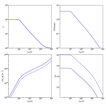
Figure 1: The evolution of the bulk Lorentz factor ($\Gamma$, upper-left panel), the co-moving frame magnetic field strength ($B^{\prime}$, upper-right panel), the injection rate of electrons ($\frac{dN_{\mathrm{e}}}{dt}$, lower-left panel), and the minimum Lorentz factor of the injected non-thermal electrons ($\gamma_{\mathrm{nth}}$, lower-right panel). This figure is plotted for a jet expanding in a homogeneous interstellar medium with $\delta=1$ (solid curve) or $\delta=0.2$ (dashed curve).

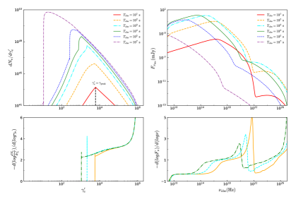
Figure 2: The evolution of the distribution function of electrons (upper-left panel) and the afterglow spectrum (upper-right panel) in the interstellar medium case with $\delta=1$. The power-law indices of the distribution function and the afterglow spectrum are shown correspondingly in the lower panels. The characteristic Lorentz factor $\gamma_{\mathrm{peak}}$ is marked in the upper-left panel.

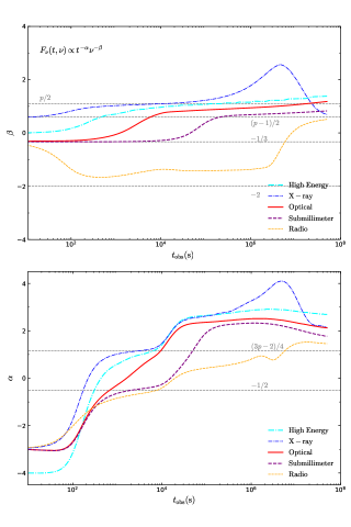
Figure 3: Evolution of the spectral index $\beta$ and the temporal indices $\alpha$ at various wavelengths ranging from high energy $\gamma$-rays (GeV) to radio bands, for the homogeneous interstellar medium case with $\delta=1$.

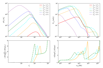
Figure 4: Same as in Figure 2, except that the $\delta$ parameter is taken as $\delta=0.2$.

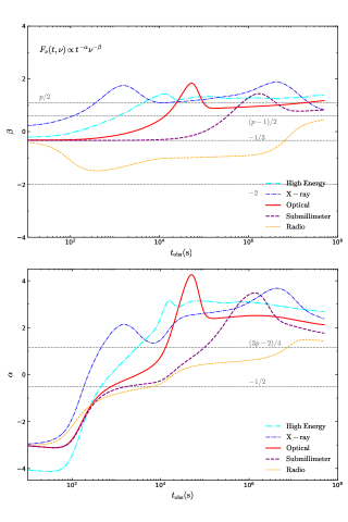
Figure 5: Same as in Figure 3, except that the $\delta$ parameter is taken as $\delta=0.2$.

3.2 Homogeneous Interstellar Medium Case

In this section, we consider the case that the GRB occurs in a homogeneous interstellar medium. The generical dynamical equations proposed by Huang et al. (2000) are adopted to depict the deceleration of the external shock. Typical values are taken for the various parameters involved. For example, the redshift of the GRB is taken as $z=1$; The half-opening angle of the jet is assumed to be $\theta_{\mathrm{j}}=2^{\circ}$, with an isotropic equivalent kinetic energy of $E=10^{53}$ erg; The initial Lorentz factor of the jet is adopted as $\Gamma=300$; Microphysical parameters characterizing the energy fractions of electrons and the magnetic field are taken as $\epsilon_{\text{e}}=0.2$ and $\epsilon_{B}=0.01$, respectively; The number density of the interstellar medium is set as $n=1.0\ \text{cm}^{-3}$. Finally, the power-law index of the electron distribution function is $p=2.2$. Various PIC simulations indicate that the power-law component of electrons accelerated by shocks can take a fraction of 10 – 20 percent of the total energy (Spitkovsky, 2008a, b; Martins et al., 2009; Sironi et al., 2013). Here, the energy fraction is defined as:

$$\delta=\frac{\int_{\gamma_{\mathrm{nth}}}^{\infty}\gamma_{\mathrm{e}}Q\left(\gamma_{\mathrm{e}},t\right)d\gamma_{\mathrm{e}}}{\int_{1}^{\infty}\gamma_{\mathrm{e}}Q\left(\gamma_{\mathrm{e}},t\right)d\gamma_{\mathrm{e}}}.$$ (13)

In our study, two different values are assumed for the energy fraction, i.e. $\delta=0.2$ and $\delta=1$.

Figure 1 shows the evolution of four parameters: the bulk Lorentz factor ($\Gamma$) of the jet, the co-moving magnetic field strength ($B^{\prime}$), the injection rate ($\frac{dN_{\mathrm{e}}}{dt}$) of electrons, and the minimum Lorentz factor ($\gamma_{\mathrm{nth}}$) of injected non-thermal electrons. Notably, we see that $\gamma_{\mathrm{nth}}$ evolves significantly in the process. At the early stage, when the observer’s time ($t_{\mathrm{obs}}$) is less than $10^{2}$ s, $\Gamma$, $B^{\prime}$, and $\gamma_{\mathrm{nth}}$ remain constant. However, the injection rate ($\frac{dN_{\mathrm{e}}}{dt}$) increases quickly by more than two orders of magnitude during this period. After $10^{2}$ s, the jet enters the deceleration phase so that $\Gamma$, $B^{\prime}$, and $\gamma_{\mathrm{nth}}$ begin to decrease continuously. The increase of $\frac{dN_{\mathrm{e}}}{dt}$ also becomes slower. Comparing with the case of $\delta=1$, the evolution of the bulk Lorentz factor and the co-moving magnetic field strength is similar when $\delta=0.2$. The presence of thermal electrons alters the distribution of accelerated electrons, leading to a change in the injection rate and the $\gamma_{\mathrm{nth}}$ parameter.

The evolution of the electron distribution and afterglow spectrum are shown in Figure 2. At the early stage, the cooling of electrons is dominated by adiabatic expansion since the jet radius is small. The energy loss rate of electrons with Lorentz factor lower than $\gamma_{\mathrm{nth}}$ is very small, while the injection rate ($\frac{dN_{\mathrm{e}}}{dt}$) continues to grow. This leads to a spike in the electron distribution at $t_{\mathrm{obs}}=10$ s. After that, with the expansion of the jet radius, synchrotron cooling becomes dominant in the lower energy segment. Concurrently, the total number of previously injected electrons is so large that the newly injected electrons are ineffective in reshaping the electron distribution. As a result, low-energy electrons exhibit a broken power-law distribution at $t_{\mathrm{obs}}=10^{7}$ s. As the electrons lose their energy through radiation, the peak frequency becomes smaller. The GeV emission initially increases (from $t_{\mathrm{obs}}=10$ s to $t_{\mathrm{obs}}=10^{3}$ s) due to the electron injection. However, it subsequently declines since the peak frequency of synchrotron emission is decreasing.

The lower-left and lower-right panels of Figure 2 shows the power-law indices of the electron distribution and the afterglow spectrum, respectively. Note that the afterglow spectrum is comprised of two distinct components, i.e., the synchrotron radiation component and the inverse Compton scattering component. Quick variation of the spectral index occurs in the high-frequency range, which could be clearly seen in the lower-right panel as a clear bump.

The evolution of the spectral index ($\beta$) at various wavelengths (from GeV to radio bands) is illustrated in the upper panel of Figure 3. Theoretically, the spectral index can be derived by considering the evolution of several characteristic frequencies, which gives (Zhang et al., 2006)

$$\beta=\begin{cases}-2,&\nu<\nu_{\mathrm{a}},\\ -\frac{1}{3},&\nu_{\mathrm{a}}<\nu<\nu_{\mathrm{m}},\\ \frac{p-1}{2},&\nu_{\mathrm{m}}<\nu<\nu_{\mathrm{c}},\\ \frac{p}{2},&\nu>\nu_{\mathrm{c}},\end{cases}$$ (14)

where $\nu_{a}$ and $\nu_{c}$ represent the self-absorption frequency and cooling frequency, respectively. In the upper panel, four horizontal dashed lines corresponding to $\beta=p/2$, $\beta=(p-1)/2$, $\beta=-1/3$, and $\beta=-2$ are also shown for a direct comparison. The peak frequency of the synchrotron self-Compton (SSC) emission is initially close to the GeV band, which makes the GeV spectral index be nearly zero. Later, the index gradually increases and eventually exceeds $p/2$. The spectral index in the X-ray band evolves from $(p-1)/2$ to $p/2$ as $\nu_{c}$ crosses this frequency range. Then it surpasses $p/2$ and reaches a maximum value at $\sim 4\times 10^{6}$ s, which corresponds to the bump in the power-law indices of the afterglow spectrum as shown in Figure 2. The evolution of the spectral indices in the optical and submillimeter bands also has two distinct plateau phases as the characteristic frequencies traverse the corresponding bands. However, the spectral index in the radio band exhibits a different evolution pattern due to the synchrotron self-absorption (SSA) effect. It first decreases, then comes to a plateau phase, and finally it rises again. Note that since the radio frequency is slightly larger than the self-absorption frequency, the spectral index remains above $-2$ all the time.

The evolution of the temporal indices at different frequencies is shown in the lower panel of Figure 3. When $t_{\mathrm{obs}}\lesssim 100$ s, the number of injected electrons is so small that the injection plays a more important role than the cooling process so that the source term in Equation (12) becomes dominant. In this period, the sign of $\alpha$ is opposite to that of $\beta$. As the number of injected electrons increases, it dominates the advection term in Equation (12), which makes the index transit from a negative value to a positive value. The index in the X-ray band shows a second plateau when $\beta$ approaches $p/2$ at $t_{\mathrm{obs}}\sim 10^{3}$ s. When $t_{\mathrm{obs}}\gtrsim 5\times 10^{3}$ s, the peak Lorentz factor ($\gamma_{\mathrm{peak}}$, see Figure 2) of electrons surpasses the value of $\gamma_{\mathrm{nth}}$. Note that the Lorentz factor of the injected electrons is typically $\gamma_{\mathrm{nth}}$ ($Q_{\mathrm{inj}}\propto\gamma_{\mathrm{nth}}^{-p}$). After that, the electron injection declines rapidly, leading to a reduction in the contribution of the source term. As a result, $\alpha$ enters a plateau phase. When $t_{\mathrm{obs}}\gtrsim 4\times 10^{6}$ s, the source term becomes negligible, leading to a bump in the evolution curve of $\alpha$, which is a counterpart of that observed in the upper panel. The timing index of the GeV emission follows a similar evolution to that of the X-ray band, because GeV photons are originated from X-ray photons up-scattered by energetic electrons. In the submillimeter band, the timing index exhibits a plateau at $\alpha=-1/2$, which corresponds to a spectral index of $\beta=-1/3$. It is followed by a second plateau phase at $t_{\mathrm{obs}}\approx 10^{5}$ s. The timing index of radio emission also shows a plateau at around $-1/2$. It slowly rises after $\sim 2\times 10^{4}$ s and eventually shows a second plateau at $10^{7}$ s. Generally, the evolution of the timing index of optical afterglow is between those of the X-ray band and the submillimeter band.

The evolution of the electron distribution and afterglow spectrum in the case of $\delta=0.2$ is shown in Figure 4. In the low-energy range where the Maxwellian distribution takes on a quadratic function form, the cooling of electrons is negligible so that they follow a power-law distribution. The transition between the Maxwellian component and the power-law component naturally leads to a relatively large power-law index of the electron distribution function. Since the afterglow spectrum completely depends on the electron distribution, we see that the spectral index near $10^{16}$ Hz increases markedly at $t_{\mathrm{obs}}=10^{3}$ s. In the lower-right panel of Figure 4, there is an obvious bump-like structure at $\sim 10^{19}$ Hz. It is due to the superposition of the synchrotron radiation and SSC emission. The photons of $\sim 10^{16}$ Hz can be up-scattered by energetic electrons through the SSC process, which leads to another bump at $\sim 10^{25}$ Hz.

The evolution of the spectral and temporal indexes in different bands in the case of $\delta=0.2$ is presented in Figure 5. The X-ray spectral index shows a non-monotonic hard-soft-hard variation during the plateau phase observed in the case of $\delta=1$. The second bump in the X-ray band is similar to that in the $\delta=1$ scenario. There is also a less evident bump in the GeV range. Both the optical and sub-millimeter spectral indices exhibit similar bumps during the late stage. Due to the SSA effect, the evolution of the radio band spectral index is similar to that when $\delta=1$. The lower panel of Figure 5 shows the evolution of the temporal index ($\alpha$). We see that when the spectral index ($\beta$) rises, the temporal index generally also increases. This could be an important indication of the thermal electrons.

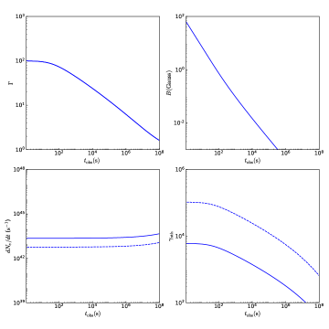
Figure 6: The evolution of the bulk Lorentz factor ($\Gamma$, upper-left panel), the co-moving frame magnetic field strength ($B^{\prime}$, upper-right panel), the injection rate of electrons ($\frac{dN_{\mathrm{e}}}{dt}$, lower-left panel), and the minimum Lorentz factor of the injected non-thermal electrons ($\gamma_{\mathrm{nth}}$, lower-right panel). This figure is plotted for a jet expanding in a stellar wind medium with $\delta=1$ (solid curve) or $\delta=0.2$ (dashed curve).

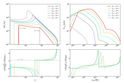
Figure 7: The evolution of the distribution function of electrons (upper-left panel) and the afterglow spectrum (upper-right panel) in the stellar wind medium case with $\delta=1$. The power-law indices of the distribution function and the afterglow spectrum are shown correspondingly in the lower panels. The characteristic Lorentz factors of $\gamma_{\mathrm{min}}$ and $\gamma_{\mathrm{nth}}$ are marked in the upper-left panel.

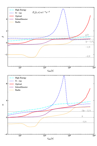
Figure 8: Evolution of the spectral index $\beta$ and the temporal indices $\alpha$ at various wavelengths ranging from high energy $\gamma$-rays (GeV) to radio bands, for the stellar wind medium case with $\delta=1$.

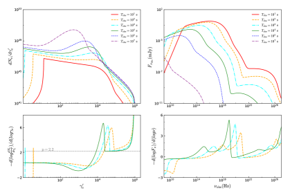
Figure 9: Same as in Figure 7, except that the $\delta$ parameter is taken as $\delta=0.2$.

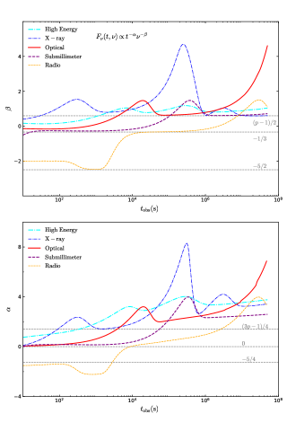
Figure 10: Same as in Figure 8, except that the $\delta$ parameter is taken as $\delta=0.2$.

3.3 Stellar Wind Medium Case

In this subsection, we present our numerical results on GRBs that occur in a stellar wind environment. Again we consider two values for the $\delta$ parameter, i.e. $\delta=0.2$ and $\delta=1$. The energy fraction of the magnetic field is taken as $\epsilon_{B}=10^{-4}$. The density of the stellar wind is assumed to take the form of $n(r)=3\times 10^{35}A_{\star}r^{-2}\ \text{cm}^{-3}$, where $A_{\star}$ is a normalization constant of the wind density which is taken as $A_{\star}=1\times 10^{-2}$. Other parameters are the same as those taken in the previous subsection.

Figure 6 shows the evolution of four parameters: the bulk Lorentz factor ($\Gamma$) of the jet, the co-moving magnetic field strength ($B^{\prime}$), the injection rate ($\frac{dN_{\mathrm{e}}}{dt}$) of electrons, and the minimum Lorentz factor ($\gamma_{\mathrm{nth}}$) of injected non-thermal electrons. Two cases of $\delta=1$ and $\delta=0.2$ are considered in our calculations. After a short coasting phase, the bulk Lorentz factor begins to decrease at 10 seconds. The magnetic field decays monotonously, but its initial value is higher than that of the homogeneous interstellar medium case. The injection rate of electrons only varies in a narrow range. Meanwhile, the Lorentz factor of $\gamma_{\mathrm{nth}}$ also decays monotonously.

The evolution of the electron distribution function and the afterglow spectrum is illustrated in Figure 7. Since the magnetic field strength here is larger than that of the homogeneous interstellar medium scenario, the cooling of low-energy electrons is more pronounced than that in Figure 2, leading to a broken power-law function for the electron distribution. As $\gamma_{\mathrm{nth}}$ slowly decreases, the injection process begins to affect the electron distribution and results in an upward warp, which emerges as a noticeable bulge at around $10^{7}$ seconds. Comparing with the interstellar medium case, there is a similar bump in the lower-right panel, which shows the evolution of the spectral index of the multi-band afterglow.

The upper panel of Figure 8 illustrates the evolution of $\beta$. The X-ray spectral index is initially between $p/2$ and $(p-1)/2$. It reaches a peak value of nearly 6 at around $2\times 10^{5}$ s, and then returns to $(p-1)/2$ later. In the GeV band, the evolution of the spectral index is very flat. It approximately equals to $(p-1)/2$ all the time. The index in the optical band is negative initially. It gradually increases between 100 — 1000 s, and keep to be about $(p-1)/2$ during $10^{3}$ — $10^{6}$ s. Then the optical index increases significantly at later stages. The spectral index in the sub-millimeter band is initially $-1/3$. It increases to $(p-1)/2$ at around $10^{4}$ s and remains constant thereafter.

Theoretically, when $\nu_{c}<\nu_{a}<\nu_{m}$, the spectral index should take the values of $-2,-5/2,1/2$, and $p/2$ successively from high frequency regime to low frequency regime. On the other hand, when $\nu_{a}<\nu_{c}<\nu_{m}$, the index should vary as $-2,-1/3,1/2$, and $p/2$ from high to low frequency. In the radio bands, the increasing jet radius causes a reduction in the electron density and leads to a decrease in the SSA frequency. Furthermore, the cooling of electrons changes their distribution. Consequently, the evolution of the radio band spectral index becomes very complicated. In Figure 8, we see that the radio-band spectral index experiences three distinct plateau phases. Initially, radio waves are emitted by electrons whose Lorentz factor is approximately $\gamma_{\mathrm{min}}$ (see the upper left panel of Figure 7), leading to a spectral index of $-2$ due to the SSA process. As the magnetic field strength declines, radio waves are emitted mainly by non-thermal electrons which obeys a power-law distribution, but not by the monochromatic electrons at $\gamma_{\mathrm{min}}$. The spectral index correspondingly changes to $-5/2$. After that, radio waves will mainly come from those electrons with the Lorentz factor concentrating at $\gamma_{\mathrm{nth}}$. By this time, the jet radius has grown significantly, rendering the impact of SSA negligible and resulting in a radio spectral index of $-1/3$. Finally, radio waves will come from those electrons with the Lorentz factor larger than $\gamma_{\mathrm{nth}}$, which essentially follow a power-law distribution of $\frac{dN_{\mathrm{e}}}{d\gamma_{\mathrm{e}}^{\prime}}\propto\gamma_{\mathrm{e}}^{\prime-p}$, then we have a radio spectral index of $(p-1)/2$. The above evolution pattern of the radio spectral index can be clearly seen in Figure 8.

The upper panel of Figure 8 shows the evolution of the temporal index $\beta$. Here, the magnetic field strength is larger than that of the homogeneous interstellar medium scenario, and the advection term in Equation 12 is dominant even in the early stage. As a result, the sign of $\beta$ is the same as that of $\alpha$. Again, we see a similar bump in the X-ray band as that of the interstellar medium case. In optical and radio bands, the evolution of the temporal index shows a clear correlation with that of the spectral index when comparing the two panels of Figure 8.

The evolution of the electron distribution function and the afterglow spectrum is illustrated in Figure 9 for the scenario of $\delta=0.2$. The upper-left panel clearly shows that the electron distribution is a combination of a power-law component and a Maxwellian component. Consequently, there is a noticeable bulge structure in the lower-left panel which shows the electron distribution index versus the Lorentz factor. The lower-right panel shows the spectral index at different frequency. Again, several distinct bulges can be seen in the plot. For example, at $t_{\mathrm{obs}}=10^{2}$ s, the existence of thermal electrons results in the first bulge at $\sim 10^{18}$ Hz. The second bulge at $\sim 10^{21}$ Hz is caused by the overlapping of the SSC and synchrotron emissions. Finally, since the SSC emission strongly depends on the electron distribution and seed synchrotron photons, the first bulge (at $\sim 10^{18}$ Hz) leads to a third bulge at $\sim 10^{26}$ Hz.

The evolution of the spectral and temporal indices is illustrated in Figure 10 for the scenario of $\delta=0.2$. In the upper panel, the bump at $t_{\mathrm{obs}}=10^{2}$ s in X-ray band is induced by the bulge of the electron distribution index (see the lower-left panel of Figure 9). It could be regarded as a signature for the existence of thermal electrons. Similarly, in optical, sub-millimeter, and radio bands, a bump can be seen at $t_{\mathrm{obs}}\sim 2\times 10^{4}$ s, $4\times 10^{5}$ s and $2\times 10^{7}$ s, respectively. In the lower panel of Figure 10, the evolution of the temporal index shows an obvious correlation with that of the corresponding spectral index. In each band, the temporal index exhibits similar bump-like structure as the spectral index.

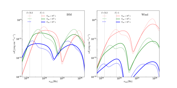
Figure 11: The afterglow spectra at three representative moments. The left panel shows the homogeneous interstellar medium cases and the right panel shows the stellar wind cases. The dotted lines correspond to $\delta=0.2$, and the solid lines correspond to $\delta=1$. Two dashed vertical lines represent the optical band and the soft X-ray band, respectively.

3.4 Afterglow Spectrum

The effects of thermal electrons on the evolution of the spectral and temporal indices have been discussed in the previous subsections. Here we further examine the influence of thermal electrons on the afterglow spectrum. Figure 11 shows the $\nu F_{\nu}$ spectrum of the afterglow for both the homogeneous interstellar medium scenarios and the stellar wind medium scenarios. Again, two conditions of $\delta=1$ and $\delta=0.2$ are considered. Generally, from these plots, we can see two distinct components in the spectrum, which correspond to the synchrotron emission and the SSC emission respectively. For the homogeneous interstellar medium case, when the effect of thermal electrons is negligible, the spectrum of the synchrotron emission is very flat and spans 4 – 5 orders of magnitudes in frequency range. On the contrary, the effect of thermal electrons mainly shows up as a peak in the low frequency region.

The spectra of the stellar wind scenarios are shown in the right panel of Figure 11. When $\delta=1$, since the electrons follow a broken power-law distribution, the synchrotron emission correspondingly shows a clear break in the spectrum (also see Figure 9). However, when $\delta=0.2$, the spectrum is clearly different, which has a bump in both the synchrotron and SSC component at $t_{\mathrm{obs}}=10^{2}$ s. At later stages, the bump structure becomes even more prominent. It could be regarded as a clear indication for the existence of thermal electrons.

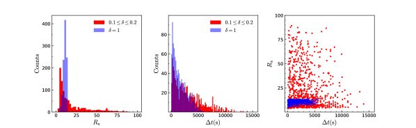
Figure 12: The distribution of simulated GRB afterglows. The left panel shows the histograms of the peak flux ratio ($R_{\mathrm{X}}$) between soft X-ray (10 keV) and hard X-ray (100 keV) emissions for simulated GRBs. The middle panel displays the histograms of the time delay between the peak times of soft X-ray and optical bands. The right panel presents the distribution of the bursts on the $R_{\mathrm{X}}$-$\Delta t$ plane. The blue dots or histograms correspond to GRBs simulated with $\delta=1$, while the red dots or histograms represent GRBs with $0.1\leq\delta\leq 0.2$.

4 Distribution of some observable parameters

In order to help find more credible evidence of the existence of thermal electrons through observations, we have conducted Monte Carlo simulations to generate a large number of GRBs. The observable parameters of their afterglows are then analyzed and their distributions are carefully examined. In our simulations, the isotropic equivalent kinetic energy ($E$) is fixed at $10^{53}$ erg and the redshift is assumed to be $z=1$. Two conditions are considered for the energy fraction ($\delta$): (i) fixed as $\delta=1$; (ii) or a homogeneous distribution in the range of $0.1\leq\delta\leq 0.2$. The reason for the latter condition is that it is supported by some recent PIC simulations (Spitkovsky, 2008a, b; Martins et al., 2009; Sironi et al., 2013). One thousand GRBs are generated under each conditions. For simplicity, we assume that the circum-burst medium is homogeneous and do not consider the stellar wind medium cases. Other parameters involved in the simulations are assumed to follow uniform distributions as: $100\leq\Gamma\leq 300$, $0.01\leq\epsilon_{\mathrm{e}}\leq 0.5$, $10^{-3}\leq\epsilon_{B}\leq 10^{-1}$, and $0.1$ cm${}^{-3}\leq n_{0}\leq 10$ cm^-3.

We mainly analyzed two parameters that can be directly measured through future afterglow observations: the peak flux ratio ($R_{\mathrm{X}}$) between soft X-ray (10 keV) and hard X-ray (100 keV) emissions, and the time delay ($\Delta t$) between the peak times of soft X-ray and optical bands. These two parameters are calculated for each simulated GRB. Figure 12 shows the frequency histograms for the peak flux ratio and the time delay. It also illustrates the distribution of all the mock GRBs in the $R_{\mathrm{X}}$-$\Delta t$ parameter space.

The left panel of Figure 12 shows the histograms of $R_{\mathrm{X}}$ for simulated GRBs. When there are no thermal electrons so that all the electrons follow a pure power-law distribution, a rough upper limit of $\sim 20$ can be noticed for the flux ratio. On the contrary, when thermal electrons are present, there should be a large number of lower energy electrons. As a result, the hard X-ray emission will be suppressed while the soft X-ray emission will be enhanced. Consequently, $R_{\mathrm{X}}$ will be significantly increased. In the left panel, we could see that for the pure non-thermal electron scenarios ($\delta=1$, blue histograms), all GRBs have a flux ratio roughly less than $\sim 20$. On the other hand, for the hybrid electron scenarios with both thermal and non-thermal electrons ($0.1\leq\delta\leq 0.2$), a significant number of GRBs (about $\sim 40\%$) have a flux ratio approximately larger than $\sim 20$.

The middle panel shows the histograms of the time delay for simulated GRBs. For the pure non-thermal electron scenarios ($\delta=1$, blue histograms), the upper limit for $\Delta t$ is approximately $\sim 6000$ s. As the peak frequency of the afterglow spectrum crosses the frequency of optical emission, the optical emission will reach its peak flux. However, When other model parameters are consistent, the initial peak Lorentz factor ($\gamma_{\mathrm{peak}}$) of the electron distribution for the hybrid electron scenario is always larger than that for the pure non-thermal electron scenario. Then the optical emission for the hybrid electron scenario will reach its peak flux at a later time. Consequently, for the hybrid electron scenarios, the time delay can exceed $\sim 6000$ s (with a percentage of $\sim 20\%$).

The right panel shows the distribution of the bursts on the $R_{\mathrm{X}}$-$\Delta t$ plane. The presence of thermal electrons significantly raise the upper limits of both $R_{\mathrm{X}}$ and $\Delta t$. Then the distribution of the GRB afterglows with thermal electrons is more dispersive in the $R_{\mathrm{X}}$-$\Delta t$ plane.

5 Observability

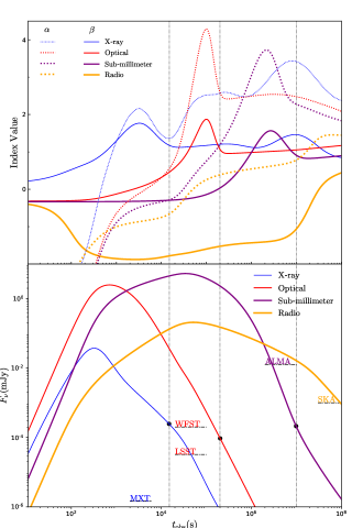
Figure 13: The evolution of the spectral and temporal indices at various wavelengths ranging from X-ray to radio bands, as well as the corresponding light curves, for the homogeneous interstellar medium case with $\delta=0.2$. The end times of the spectral indices decline for three bands are shown by dashed vertical lines, and the corresponding flux of these bands is marked by black dots. The sensitivities of several telescopes/detectors are also marked as a direct comparison, including the MXT, LSST, WFST, ALMA, and SKA.

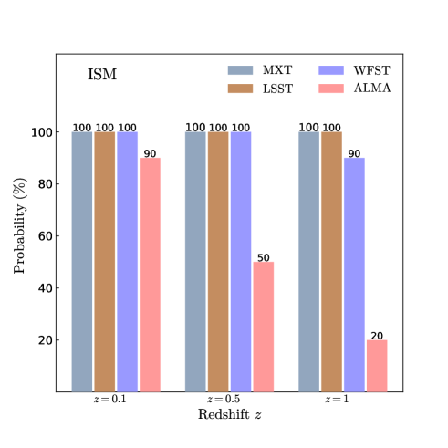
(a)

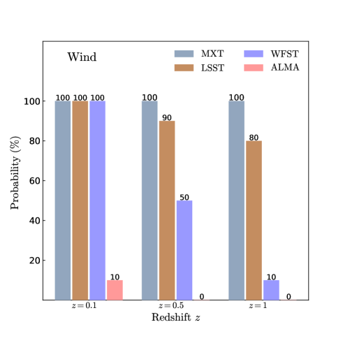
(b)

Figure 14: The optimistic detection probability of several telescopes/detectors, including the MXT, LSST, WFST, and ALMA, for detecting the thermal electron signals with spectral and timing indices in the ideal observation situation. The left panel shows the homogeneous interstellar medium cases and the right panel shows the stellar wind cases.

5.1 single-band observability

As shown in Section 3, the simultaneous occurrence of bumps in both the spectral and temporal indices can serve as an indication of the presence of thermal electrons. However, measuring these indices requires that the radiation flux should be higher than the sensitivity of the detectors. In this subsection, we discuss the single-band observability of GRB afterglows by various telescopes/detectors in the ideal observation situation.

Figure 13 shows the evolution of the spectral and temporal indices as well as the corresponding muti-band light curves. The sensitivities of several telescopes/detectors are also marked for a direct comparison, including the Microchannel X-ray Telescope (MXT) on board the Space Variable Objects Monitor (SVOM), Wide Field Survey Telescope (WFST), Vera Rubin Observatory Legacy Survey of Space and Time (LSST), Atacama Large Millimeter/submillimeter Array (ALMA), and Square Kilometre Array (SKA). Note that the exposure time is taken as 100 s for MXT, 3 hr for LSST and WFST, 4 hr for ALMA, and 1 hr for SKA.

As is shown in Figure 13, in order to observe the whole thermal-electron signal with the spectral and timing indices, the detection threshold of the detector must be lower than the radiation flux before the spectral indice decline ends. However, due to the cooling of electrons, the appearance time of the thermal-electron signals in the lower energy bands is late. The thermal-electron signals did not appear in the spectral/timing indices of the radio band when $t_{\mathrm{obs}}\sim 10^{8}$ s, although the radio flux has been below the detection threshold of the SKA. It is hard to identify the signal of thermal electrons from the radio band.

To obtain the detection probability for identifying thermal electrons by observing non-monotonic changes in the spectral and temporal indices in a single band, we ran 1000 Monte Carlo simulations for various redshifts (including z = 0.1, z = 0.5, and z = 1) and different circumburst medium (the homogeneous interstellar and stellar wind media). For the homogeneous interstellar medium case, the model parameters used are identical to those in Section 4. For the stellar wind medium case, parameters involved in the simulations are also assumed to follow uniform distributions as: $100\leq\Gamma\leq 300$, $0.01\leq\epsilon_{\mathrm{e}}\leq 0.5$, $10^{-4}\leq\epsilon_{B}\leq 10^{-2}$, and $10^{-2}\leq A_{\star}\leq 10^{0}$.

The probability of detecting thermal electron signals by different detectors is displayed in the Figure 14. For the homogeneous interstellar medium case (see the left panel of Figure 14), the optimistic probabilities of the MXT, LSST, WFST and ALMA identifying the thermal electron signal from a burst with a redshift of $z\sim 1$ are 100%, 100%, 90% and 20%.

Due to the rapid dissipation of the external shock in the stellar wind medium, the radiation flux is often below the detector’s detection threshold before the thermal electron signal appears. As is shown in the right panel of Figure 14, the MXT has an optimistic probability of 100% for identifying thermal electrons from bursts with a redshift of $z\sim 1$, owing to its excellent detection performance. The LSST has an optimistic probability of 80% for detecting thermal electrons from bursts with a redshift of $z\sim 1$, while the detection probabilities of the WFST and ALMA for the same GRB population are 10% and zero, respectively. However, the WFST has an optimistic probability of 50% for identifying the thermal electrons from the bursts with a redshift of $z\sim 0.5$.

5.2 muti-band observability

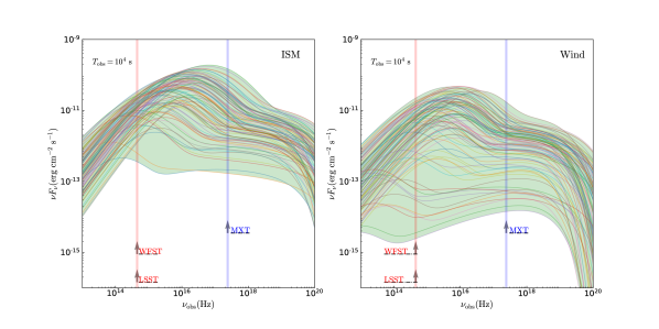
Figure 15: The Monte Carlo simulation results of the afterglow spectrum. The redshift is set as $z=1$, and the $\delta$ parameter is taken as $\delta=0.2$. The left panel shows the homogeneous interstellar medium cases and the right panel shows the stellar wind cases. The sensitivities of several telescopes/detectors are also marked as a direct comparison, including the MXT, LSST, and WFST. The green shading on the graph indicates the distribution area of the afterglow spectrum. Two transparent solid lines represent the optical band and the soft X-ray band, respectively.

There may be some challenges in identifying thermal electrons by observing non-monotonic changes in the spectral and temporal indices in a single band. For example, consecutive high-cadence and high-accuracy photometry are necessary to capture the non-monotonic variation of the temporal indices. However, there is another plausible method that identifies thermal electrons from variations of the afterglow spectrum’s structure. As is shown in Figure 11, when $t_{\mathrm{obs}}=10^{4}$ s, for the homogeneous interstellar medium case, the presence of thermal electrons causes the optical flux to exceed that of the soft X-ray, even though the optical flux is significantly lower in their absence; for the stellar wind case, the effect of thermal electrons makes the optical flux to be slightly lower than that of the soft X-ray, while it is significantly lower in the absence of thermal electrons. Thus, the ratio of the optical flux to that of the soft X-ray can be a indicator of the thermal-electron presence, and it could be derived by synergy observation in the optical (with LSST) and X-ray bands (with MXT).

To identify thermal electrons by synergy observation in the optical and X-ray bands, the optical and soft X-ray fluxes in the afterglow spectrum are required to exceed the detection threshold of LSST and MXT, respectively. Moreover, if the optical flux surpasses the flux of soft X-ray, the presence of thermal electrons can be confirmed. However, the flux ratio of between optical and soft X-ray bands in the afterglow spectrum may still be lower than 1 even if thermal electrons are present. In this scenario, the optical flux is much smaller than that of the soft X-ray when thermal electrons are absent, thus the optical flux enhanced by the presence of thermal electrons remains lower than that of the soft X-ray. The judgment for the presence of thermal electrons is set as the flux ratio is greater than 2 for good operability, although the ratio exceeding 1 is enough.

To obtain the detection probability of identifying thermal electrons by synergy observation in these two bands, 1000 Monte Carlo simulations are conducted for the homogeneous interstellar medium and stellar wind medium cases, respectively, and the results are displayed in Figure 15. The redshift is set as $z=1$, the $\delta$ parameter is taken as $\delta=0.2$, and other model parameters used are identical to those in Subsection 5.1. The optimistic detection probability is beyond 30% for both the homogeneous interstellar medium and stellar wind medium cases.

6 Conclusions and Discussion

In this study, we investigate the effects of thermal electrons on GRB afterglows. Two kinds of circum-burst medium are considered, the homogeneous interstellar medium and the stellar wind medium. An analytical expression that connects the spectral index and the temporal index is derived based on a simplified assumption that each electron emits photons mainly at a particular frequency through synchrotron radiation. It is found that a positive correlation exists between the two indices due to the cooling of electrons, which is independent on the detailed radiation mechanism. Multi-band afterglows (from X-ray to radio waves) are calculated numerically, which reveal that there exists a simultaneous bump in the evolution of both the temporal and spectral index when thermal electrons are present. The bump can serve as a crucial indicator of the presence of thermal electrons. The presence of thermal electrons also alter the afterglow spectrum. In the homogeneous interstellar medium scenarios, the synchrotron spectrum exhibits a prominent bump when thermal electrons are present. In the stellar wind medium scenarios, the synchrotron spectrum exhibits a distinctive hump-like profile due to the thermal electrons.

Monte Carlo simulations are conducted to reveal the characteristics of GRBs in some interesting observable parameters, i.e., the peak flux ratio between soft X-rays and hard X-rays, and the time delay between the peak times of soft X-rays and optical photons. When there are only non-thermal electrons, the peak flux ratio is generally less than $\sim 20$ and the time delay is less than $\sim 6000$ s. However, when thermal electrons are present, the peak flux ratio can exceed $\sim 20$ and the time delay can be larger than $\sim 6000$ s. A flux ratio exceeding $\sim 20$ or a time delay exceeding $\sim 6000$ s could be regarded as a firm evidence indicating that thermal electrons are presented in the shock.

For the ideal observation situation, the observability of the thermal electron signatures is discussed in context of typical telescopes/detectors. In the homogeneous interstellar medium cases, the MXT, LSST, WFST, and ALMA will be able to record the bump-like signatures of the spectral and temporal indices from bursts with a redshift of $z\sim 1$. In the stellar wind medium cases, the rapid decay of the afterglow generally makes it difficult to record the bump structure of the two indices. Owing to its excellent detection performance, the MXT is able to identify thermal electrons from bursts with a redshift of $z\sim 1$, while the LSST is capable of identification of thermal electrons from the same GRB population. The WFST can identify the thermal electrons from the bursts with a redshift of $z\sim 0.5$. The presence of thermal electrons can also be identified from the afterglow spectrum. For both the homogeneous interstellar medium and stellar wind medium cases, the thermal electron signatures can be diagnosed by synergy observation in the optical (with the LSST) and X-ray bands (with the MXT) from burst with a redshift of $z\sim 1$.

Identifying thermal electrons through observations still poses challenges, as it requires synchronous acquisition of multi-band data. In fact, different instruments/detectors usually perform observations at different times after the burst and at different cadences. Then obtained data may even be inconsistent with each other due to systematic difference (Gobat et al., 2023). So far, most wide-field telescopes, including WFST and LSST, can only image the observed sky area in very limited bands during a single exposure. It is not easy to get the temporal and spectral indices even in optical bands. In this aspect, the Multi-channel Photometric Survey Telescope (Mephisto) may be helpful. It has a typical $5\sigma$ r-band depth of 22.37 mag for a 40 s exposure, and can simultaneously measure the flux in three bands ($u,g,i$ or $v,r,z$). Both the temporal and spectral indices could be derived from these observations.

In reality, a number of GRBs may be missed by X-ray/gamma-ray detectors on board the satellites. Even if a GRB is triggered by these detectors, the wide-field telescope may not be able to perform timely and effective follow-up observations, due to its observatory location, weather conditions, and its own sky survey projects. Thus, the real detection probability for detectors/telescopes of identifying thermal electrons from afterglows will be less than the simulation results.

In our Monte Carlo simulations, we assume that all the dynamic parameters follow uniform distributions in particular ranges. It may differ from realistic cases. The distribution of measurable afterglow parameters could be influenced by the distribution of dynamic parameters. Further studies on these effects need to be conducted in the future.

The acceleration mechanism of particles in relativistic shocks is still under debate. Probing thermal electrons in GRB afterglows may provide vital clues for understanding the particle acceleration mechanism. Actually, there are some strange deviations from the analytical results of spectral indices in some GRB afterglows. The contribution of thermal electrons may account for these deviations (Zhang et al., 2007; Giannios & Spitkovsky, 2009; Wang et al., 2015). On the other hand, the relation between the spectral and temporal indices is related to the cooling of electrons. The observation and investigation of both the spectral and temporal indices may help reveal the detailed cooling process of electrons.

References

- Blumenthal & Gould (1970) Blumenthal, G. R., & Gould, R. J. 1970, Reviews of Modern Physics, 42, 237, doi: 10.1103/RevModPhys.42.237
- Crumley et al. (2019) Crumley, P., Caprioli, D., Markoff, S., & Spitkovsky, A. 2019, MNRAS, 485, 5105, doi: 10.1093/mnras/stz232
- Dai & Lu (1998) Dai, Z. G., & Lu, T. 1998, A&A, 333, L87, doi: 10.48550/arXiv.astro-ph/9810402
- Deng & Zhang (2014) Deng, W., & Zhang, B. 2014, ApJ, 785, 112, doi: 10.1088/0004-637X/785/2/112
- Eichler et al. (1989) Eichler, D., Livio, M., Piran, T., & Schramm, D. N. 1989, Nature, 340, 126, doi: 10.1038/340126a0
- Eichler & Waxman (2005) Eichler, D., & Waxman, E. 2005, ApJ, 627, 861, doi: 10.1086/430596
- Gao et al. (2013) Gao, H., Lei, W.-H., Zou, Y.-C., Wu, X.-F., & Zhang, B. 2013, New Astronomy Reviews, 57, 141, doi: https://doi.org/10.1016/j.newar.2013.10.001
- Gao et al. (2021) Gao, H.-X., Geng, J.-J., & Huang, Y.-F. 2021, Astronomy & Astrophysics,, 656, A134, doi: 10.1051/0004-6361/202141647
- Gao et al. (2022) Gao, H.-X., Geng, J.-J., Hu, L., et al. 2022, MNRAS, 516, 453, doi: 10.1093/mnras/stac2215
- Geng et al. (2018a) Geng, J.-J., Dai, Z.-G., Huang, Y.-F., et al. 2018a, ApJ, 856, L33, doi: 10.3847/2041-8213/aab7f9
- Geng et al. (2018b) Geng, J.-J., Huang, Y.-F., Wu, X.-F., Zhang, B., & Zong, H.-S. 2018b, ApJS, 234, 3, doi: 10.3847/1538-4365/aa9e84
- Geng et al. (2016) Geng, J. J., Wu, X. F., Huang, Y. F., Li, L., & Dai, Z. G. 2016, ApJ, 825, 107, doi: 10.3847/0004-637X/825/2/107
- Geng et al. (2014) Geng, J. J., Wu, X. F., Li, L., Huang, Y. F., & Dai, Z. G. 2014, ApJ, 792, 31, doi: 10.1088/0004-637X/792/1/31
- Giannios & Spitkovsky (2009) Giannios, D., & Spitkovsky, A. 2009, MNRAS, 400, 330, doi: 10.1111/j.1365-2966.2009.15454.x
- Gobat et al. (2023) Gobat, C., van der Horst, A. J., & Fitzpatrick, D. 2023, MNRAS, 523, 775, doi: 10.1093/mnras/stad1189
- Gould & Schréder (1967) Gould, R. J., & Schréder, G. P. 1967, Physical Review, 155, 1404, doi: 10.1103/PhysRev.155.1404
- Huang et al. (1999) Huang, Y. F., Dai, Z. G., & Lu, T. 1999, MNRAS, 309, 513, doi: 10.1046/j.1365-8711.1999.02887.x
- Huang et al. (2000) Huang, Y. F., Gou, L. J., Dai, Z. G., & Lu, T. 2000, ApJ, 543, 90, doi: 10.1086/317076
- Kobayashi & Sari (2000a) Kobayashi, S., & Sari, R. 2000a, in American Institute of Physics Conference Series, Vol. 526, Gamma-ray Bursts, 5th Huntsville Symposium, ed. R. M. Kippen, R. S. Mallozzi, & G. J. Fishman, 550–554, doi: 10.1063/1.1361598
- Kobayashi & Sari (2000b) Kobayashi, S., & Sari, R. 2000b, ApJ, 542, 819, doi: 10.1086/317021
- Kumar & Zhang (2015) Kumar, P., & Zhang, B. 2015, Phys. Rep., 561, 1, doi: 10.1016/j.physrep.2014.09.008
- Li et al. (2019) Li, L.-B., Geng, J.-J., Huang, Y.-F., & Li, B. 2019, ApJ, 880, 39, doi: 10.3847/1538-4357/ab275d
- Longair (2011) Longair, M. S. 2011, High Energy Astrophysics
- Lundman et al. (2013) Lundman, C., Pe’er, A., & Ryde, F. 2013, MNRAS, 428, 2430, doi: 10.1093/mnras/sts219
- Margalit & Quataert (2021) Margalit, B., & Quataert, E. 2021, ApJ, 923, L14, doi: 10.3847/2041-8213/ac3d97
- Martins et al. (2009) Martins, S. F., Fonseca, R. A., Silva, L. O., & Mori, W. B. 2009, ApJ, 695, L189, doi: 10.1088/0004-637X/695/2/L189
- Medina Covarrubias et al. (2023) Medina Covarrubias, R., De Colle, F., Urrutia, G., & Vargas, F. 2023, arXiv e-prints, arXiv:2306.01136, doi: 10.48550/arXiv.2306.01136
- Meng et al. (2022) Meng, Y.-Z., Geng, J.-J., & Wu, X.-F. 2022, MNRAS, 509, 6047, doi: 10.1093/mnras/stab3132
- Mészáros et al. (1993) Mészáros, P., Laguna, P., & Rees, M. J. 1993, ApJ, 415, 181, doi: 10.1086/173154
- Mészáros & Rees (1997) Mészáros, P., & Rees, M. J. 1997, ApJ, 476, 232, doi: 10.1086/303625
- Paczyński (1998) Paczyński, B. 1998, ApJ, 494, L45, doi: 10.1086/311148
- Paczynski & Rhoads (1993) Paczynski, B., & Rhoads, J. E. 1993, ApJ, 418, L5, doi: 10.1086/187102
- Panaitescu (2005) Panaitescu, A. 2005, MNRAS, 363, 1409, doi: 10.1111/j.1365-2966.2005.09532.x
- Park et al. (2015) Park, J., Caprioli, D., & Spitkovsky, A. 2015, Phys. Rev. Lett., 114, 085003, doi: 10.1103/PhysRevLett.114.085003
- Pe’er et al. (2006) Pe’er, A., Mészáros, P., & Rees, M. J. 2006, ApJ, 642, 995, doi: 10.1086/501424
- Pennanen et al. (2014) Pennanen, T., Vurm, I., & Poutanen, J. 2014, A&A, 564, A77, doi: 10.1051/0004-6361/201322520
- Piran (2004) Piran, T. 2004, Reviews of Modern Physics, 76, 1143, doi: 10.1103/RevModPhys.76.1143
- Rees & Meszaros (1992) Rees, M. J., & Meszaros, P. 1992, MNRAS, 258, 41, doi: 10.1093/mnras/258.1.41P
- Rees & Mészáros (1994) Rees, M. J., & Mészáros, P. 1994, ApJ, 430, L93, doi: 10.1086/187446
- Ressler & Laskar (2017) Ressler, S. M., & Laskar, T. 2017, ApJ, 845, 150, doi: 10.3847/1538-4357/aa8268
- Rybicki & Lightman (1979) Rybicki, G. B., & Lightman, A. P. 1979, Radiative processes in astrophysics
- Sari & Piran (1999) Sari, R., & Piran, T. 1999, ApJ, 520, 641, doi: 10.1086/307508
- Sari et al. (1998) Sari, R., Piran, T., & Narayan, R. 1998, ApJ, 497, L17, doi: 10.1086/311269
- Sironi et al. (2013) Sironi, L., Spitkovsky, A., & Arons, J. 2013, ApJ, 771, 54, doi: 10.1088/0004-637X/771/1/54
- Spitkovsky (2008a) Spitkovsky, A. 2008a, ApJ, 673, L39, doi: 10.1086/527374
- Spitkovsky (2008b) —. 2008b, ApJ, 682, L5, doi: 10.1086/590248
- Spruit et al. (2001) Spruit, H. C., Daigne, F., & Drenkhahn, G. 2001, A&A, 369, 694, doi: 10.1051/0004-6361:20010131
- Tavani (1996) Tavani, M. 1996, ApJ, 466, 768, doi: 10.1086/177551
- Thompson (1994) Thompson, C. 1994, MNRAS, 270, 480, doi: 10.1093/mnras/270.3.480
- Uhm & Zhang (2014) Uhm, Z. L., & Zhang, B. 2014, Nature Physics, 10, 351, doi: 10.1038/nphys2932
- Wang et al. (2015) Wang, X.-G., Zhang, B., Liang, E.-W., et al. 2015, ApJS, 219, 9, doi: 10.1088/0067-0049/219/1/9
- Warren et al. (2018) Warren, D. C., Barkov, M. V., Ito, H., Nagataki, S., & Laskar, T. 2018, MNRAS, 480, 4060, doi: 10.1093/mnras/sty2138
- Warren et al. (2017) Warren, D. C., Ellison, D. C., Barkov, M. V., & Nagataki, S. 2017, ApJ, 835, 248, doi: 10.3847/1538-4357/aa56c3
- Yabe et al. (2001) Yabe, T., Xiao, F., & Utsumi, T. 2001, Journal of Computational Physics, 169, 556, doi: 10.1006/jcph.2000.6625
- Yu & Dai (2007) Yu, Y. W., & Dai, Z. G. 2007, A&A, 470, 119, doi: 10.1051/0004-6361:20077053
- Zhang (2018) Zhang, B. 2018, The Physics of Gamma-Ray Bursts, doi: 10.1017/9781139226530
- Zhang et al. (2006) Zhang, B., Fan, Y. Z., Dyks, J., et al. 2006, ApJ, 642, 354, doi: 10.1086/500723
- Zhang & Yan (2011) Zhang, B., & Yan, H. 2011, ApJ, 726, 90, doi: 10.1088/0004-637X/726/2/90
- Zhang et al. (2007) Zhang, B.-B., Liang, E.-W., & Zhang, B. 2007, ApJ, 666, 1002, doi: 10.1086/519548
- Zhang et al. (2011) Zhang, B.-B., Zhang, B., Liang, E.-W., et al. 2011, ApJ, 730, 141, doi: 10.1088/0004-637X/730/2/141
- Zhang et al. (2019) Zhang, Y., Geng, J.-J., & Huang, Y.-F. 2019, ApJ, 877, 89, doi: 10.3847/1538-4357/ab1b10