Efficient Generation of Multimodal Fluid Simulation Data

Abstract

Applying the representational power of machine learning to the prediction of complex fluid dynamics has been a relevant subject of study for years. However, the amount of available fluid simulation data does not match the notoriously high requirements of machine learning methods. Researchers have typically addressed this issue by generating their own datasets, preventing a consistent evaluation of their proposed approaches. Our work introduces a generation procedure for synthetic multi-modal fluid simulations datasets. By leveraging a GPU implementation, our procedure is also efficient enough that no data needs to be exchanged between users, except for configuration files required to reproduce the dataset. Furthermore, our procedure allows multiple modalities (generating both geometry and photorealistic renderings) and is general enough for it to be applied to various tasks in data-driven fluid simulation. We then employ our framework to generate a set of thoughtfully designed benchmark datasets, which attempt to span specific fluid simulation scenarios in a meaningful way. The properties of our contributions are demonstrated by evaluating recently published algorithms for the neural fluid simulation and fluid inverse rendering tasks using our benchmark datasets. Our contribution aims to fulfill the community’s need for standardized benchmarks, fostering research that is more reproducible and robust than previous endeavors.

<ccs2012> <concept> <concept_id>10010147.10010371.10010352.10010379</concept_id> <concept_desc>Computing methodologies Physical simulation</concept_desc> <concept_significance>500</concept_significance> </concept> <concept> <concept_id>10010147.10010371.10010352.10010380</concept_id> <concept_desc>Computing methodologies Motion processing</concept_desc> <concept_significance>500</concept_significance> </concept> <concept> <concept_id>10010147.10010257</concept_id> <concept_desc>Computing methodologies Machine learning</concept_desc> <concept_significance>300</concept_significance> </concept> <concept> <concept_id>10010147.10010178.10010224.10010245.10010254</concept_id> <concept_desc>Computing methodologies Reconstruction</concept_desc> <concept_significance>300</concept_significance> </concept> </ccs2012>

[500]Computing methodologies Physical simulation [500]Computing methodologies Motion processing [300]Computing methodologies Machine learning [300]Computing methodologies Reconstruction

1 Introduction

In this work, we introduce an efficient generation procedure to produce synthetic multi-modal datasets of fluid simulations, and use it to generate two thoughtfully designed benchmark datasets. The procedure can reproduce the dynamics of fluid flows and allows for exploring and learning various properties of their complex behavior, from distinct perspectives and modalities. We then demonstrate the suitability of the generated data for data-driven pipelines by training state-of-the-art fluid simulation and inverse rendering models.

Recent work in animation-based datasets greatly contributed to the development of novel, powerful data-driven models, whose goal is to solve classic problems in computer graphics more efficiently or grant completely new degrees of freedom to digital artists. A vast and well-established category of such datasets concerns skeleton-based animations of human bodies: their wide range of applications and the availability of ad-hoc technology for capturing raw data helped the diffusion of several different datasets with varied goals, among which we can note the well-known DFAUST dataset [BRPMB17]. One really successful application of human motion datasets was the creation of SMPL [LMR^∗15], a skinned multi-person linear model, which may be used for traditional skinning as well as in a generative fashion, to sample novel human poses and styles. In contrast to using motion capture systems for human motion data, capturing the complex deformations in the geometry of fluids requires specialized equipment and software, leading to a costly and time-consuming process [HHL^∗05, EUT19]. These limitations impact the variability of the distributions which may be captured by the datasets, motivating the introduction of synthetic ones which can easily span a larger space of fluid behaviours.

Our dataset is designed starting from a simple generic environment template which can be instantiated by specifying a set of variables and constants via a configuration file. These include, for instance, meshes to specify initial fluid states and boundary conditions, but also simulation parameters. The template can also be extended to account for additional features, such as initial velocities or time-varying force fields. The scenes are instantiated by combinations of the specified values for all variables, and simulated with the resulting parameters. We leverage a very efficient GPU Lattice Boltzmann implementation [Leh] to simulate our scenes, allowing for generation of large-scale datasets in just few hours. The user can also specify multiple views from which to acquire photo-realistic renders of the simulation, as well as the export format for the fluid’s geometry (allowing for both Eulerian and Lagrangian simulation data).

Our dataset could prove to be a useful tool in a variety of interesting research directions. We provide two primary examples which received significant interest from the community in recent year. The first and most straightforward one is the development of data-driven fluid simulation models. The goal of this line of research is to approximate resource-intensive fluid simulators with light-weight models, in pipelines where approximation is tolerable (e.g.computer graphics for game/movie industry). A related task, for which our dataset would also be useful, is fluid super-resolution, where a data-driven model is learned to add fine detail over coarse simulations. A second line of research is the inverse rendering/surface recovery problem, applied to scenes displaying fluid behaviour. The inverse rendering problem has been a major subject of AI and computer vision research in the last few years, since the introduction of NeRF by Mildenhall et al.[MST^∗20]. Recently, the community has attempted to apply the NeRF paradigm to multi-view videos of fluid scenes, discovering that this application is non-trivial and requires additional considerations. Secondarily, our dataset can be systematically and reliably applied in the generation of test scenes for novel fluid simulation algorithms, allowing to benchmark them against the results of a standard Lattice Boltzmann (LBM) implementation.

Overall, our work attempts to fill a long-standing gap in data-driven fluid simulation research, and we believe it could prompt novel contributions by the community as well as improve their reproducibility and soundness, allowing more thorough and systematic evaluations. Wrapping up, our contributions are three-fold:

• We introduce an efficient GPU-based tool for generating synthetic multi-modal fluid simulation data, accommodating a wide range of fluid dynamics representations.

• Leveraging this tool, we present three carefully designed benchmark datasets that address specific fluid simulation scenarios, establishing a standard for consistent research evaluations.

• We showcase the efficacy and suitability of our datasets by training state-of-the-art models for fluid simulation and inverse rendering tasks.

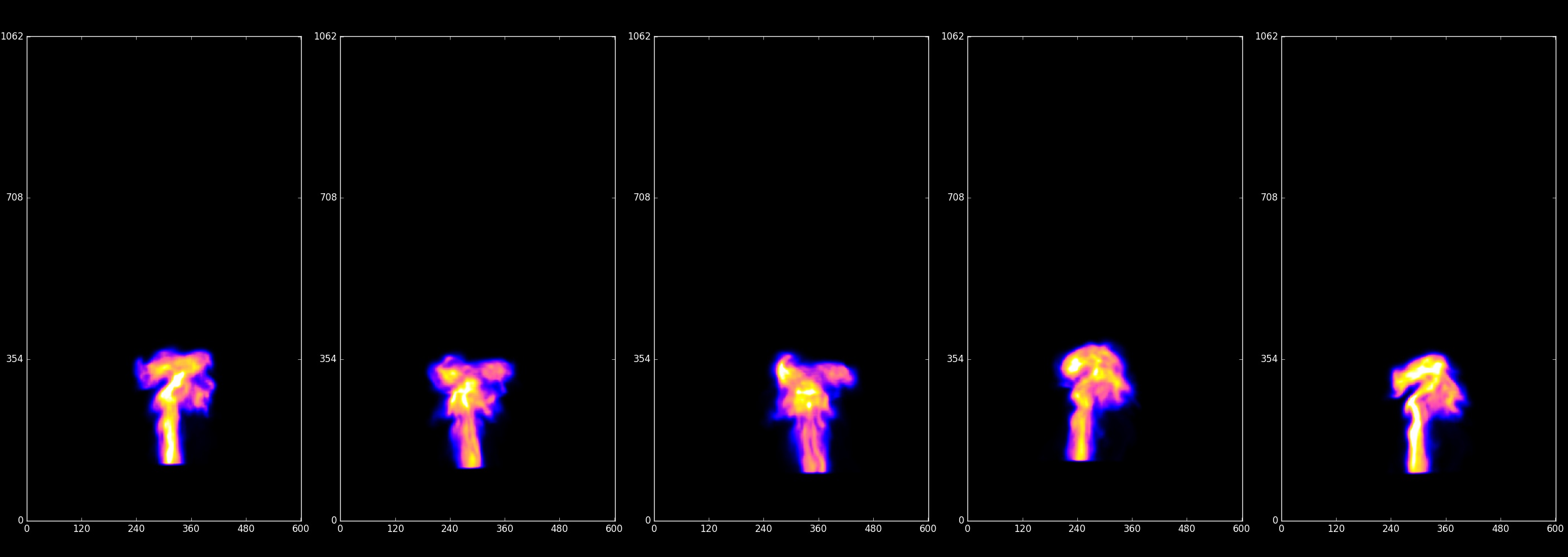
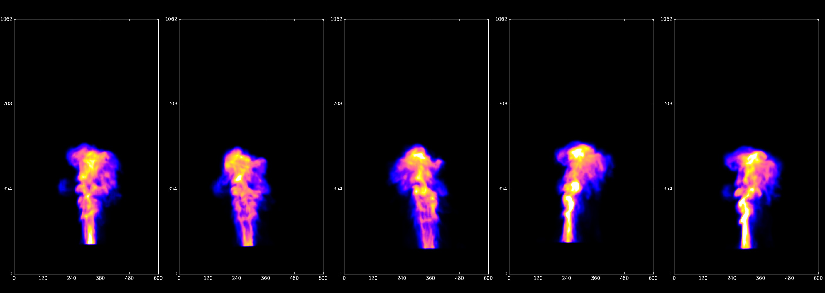
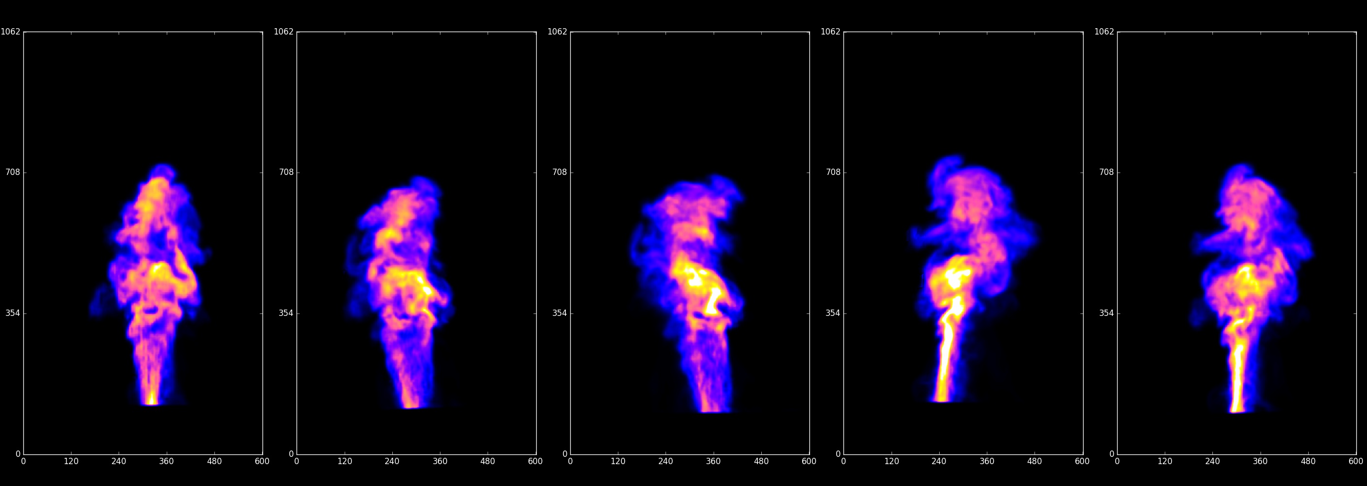
Figure 1: Multiple rendered views for three timesteps of a smoke plume simulation from the ScalarFlow [EUT19] dataset. The rendered density field is reconstructed from real smoke captures.

2 Motivation and applications

Approaches attempting to combine the descriptive power of neural networks with the simulation of fluid dynamics could significantly benefit from our dataset; we discuss interesting directions from this area of research.

Learning to predict high-resolution fluid simulations with fine detail from coarse ones is referred to as fluid super-resolution. GAN models proved especially useful in super-resolution, as showed in [WXCT19, XFCT18]. Similar works train models to upsample smoke flows and predict turbulence in smoke flows [BLDL20, BWDL21]. Further research showed how to apply the super-resolution paradigm to multi-phase flows (i.e., with multiple fluid interfaces) [LM22] and even without high-resolution labels [GSW21]. This line of research also showed promising results for physical models of biological systems [FSD^∗20].

More in general, one could exploit neural networks to learn the entire simulation model using the current fluid state as input. Much like standard simulators, this problem can be addressed in a Lagrangian or Eulerian viewpoint. The former defines the fluid dynamics on a set of particles. Ummenhofer et al. [UPTK20] first showed that continuous convolution over point sets allows to learn a lightweight and powerful model for this formulation. The work of Prantl et al. [PUKT22] improves over this contribution, introducing a momentum conservation guarantee in their model. Li et al. [LF22] showed that graph structure allowed the application of graph neural networks to particle-based fluid models, providing performance increase at virtually no quality cost. The Eulerian viewpoint, on the other hand, defines the fluid (and its properties, e.g.the velocity) as a function over the embedding space. DeepFluids[KAT^∗19] proposed a generative model of velocity fields, parametrized on the current simulation state and simulation parameters. Wievel et al. [WBT19] showed that one may consider the latent space of a generative model for simulation data, and train a model to predict consistent paths in this latent space in order to generate consistent simulations. This work was extended in [WKA^∗20] to improve stability and controllability. We refer to Vinuesa et al. [VB22] for a complete analysis about the benefits of applying learning paradigms to different stages of fluid simulations.

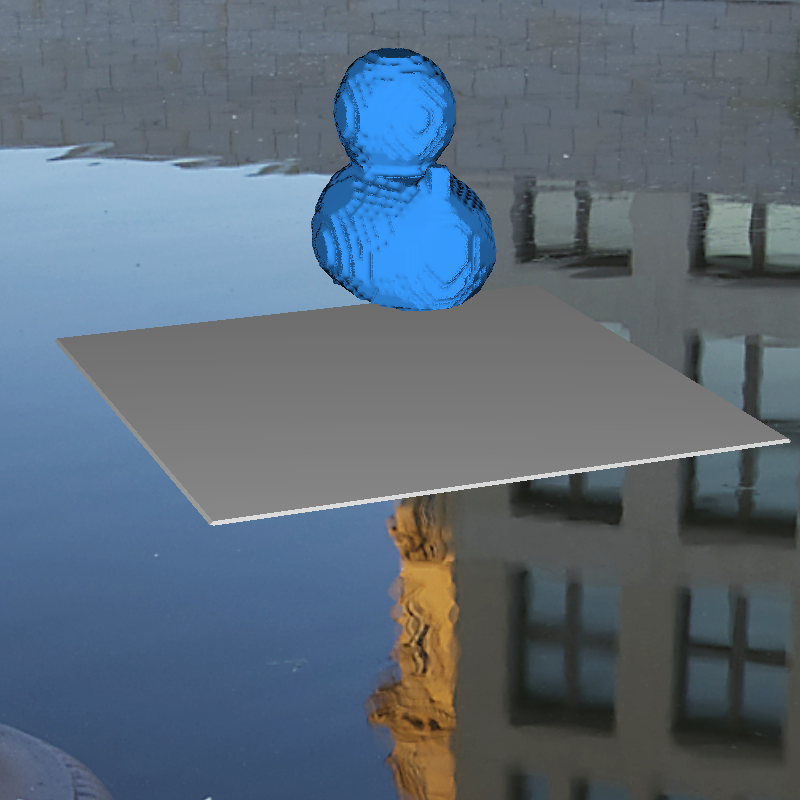
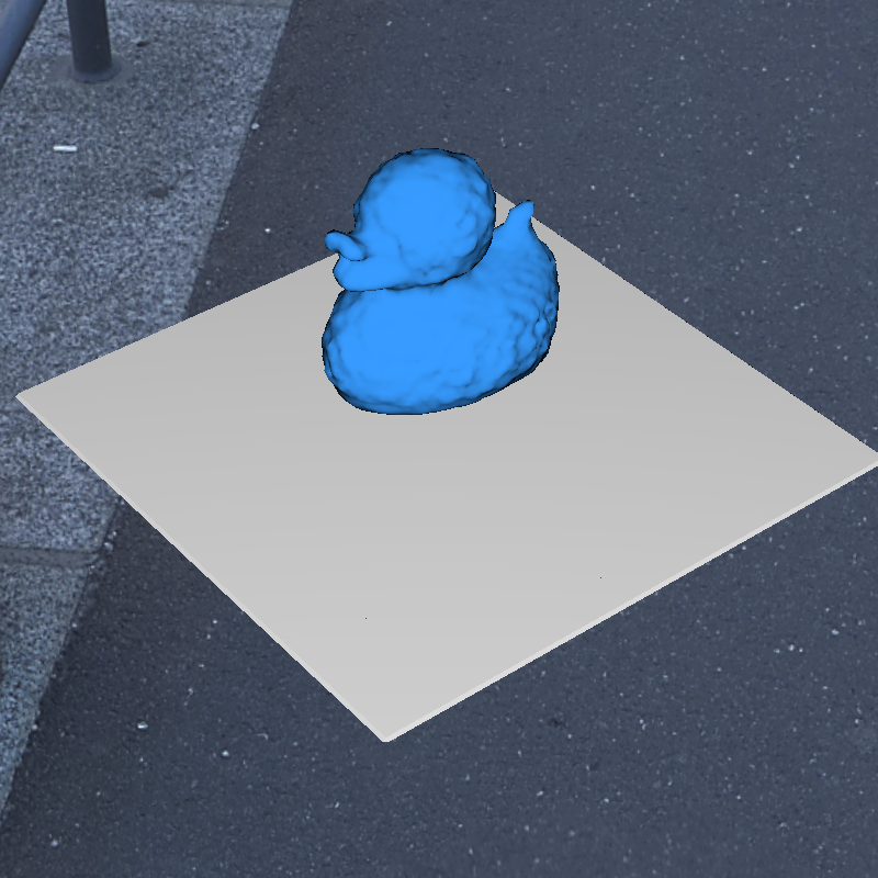
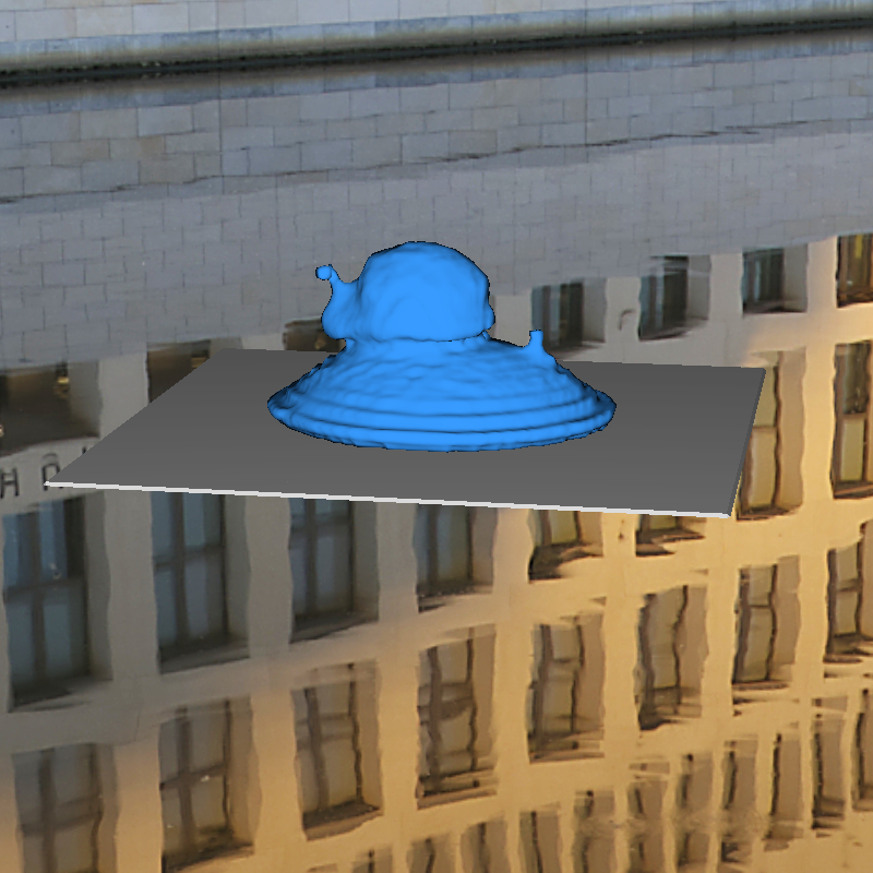
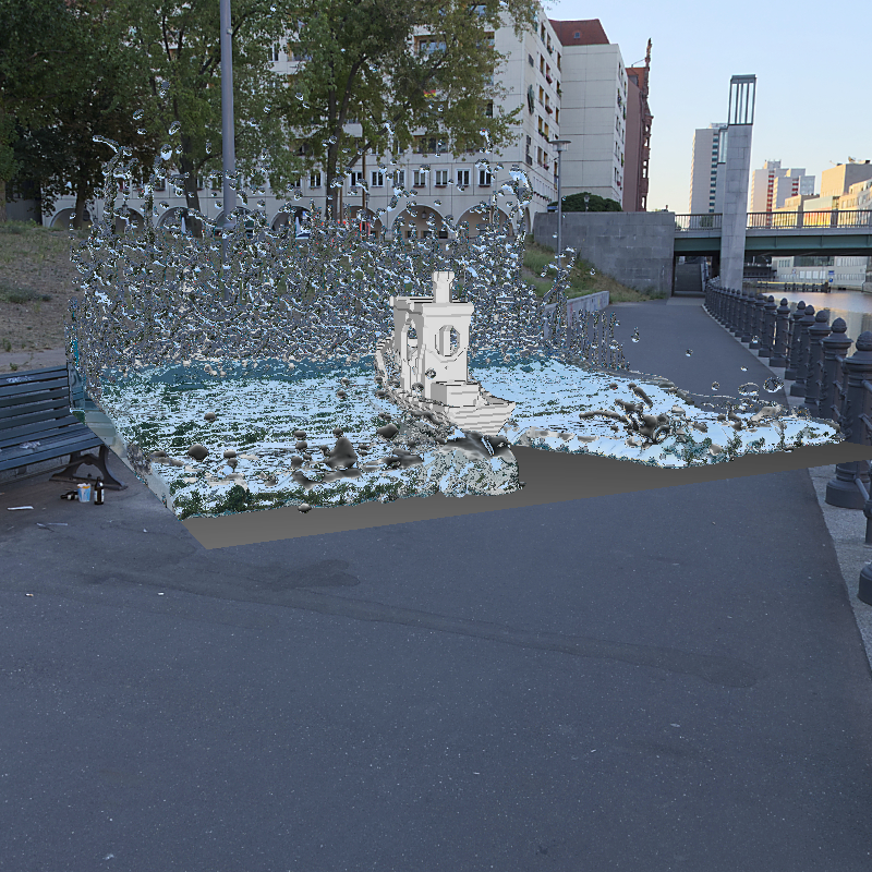
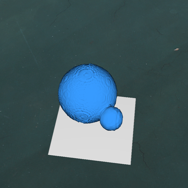
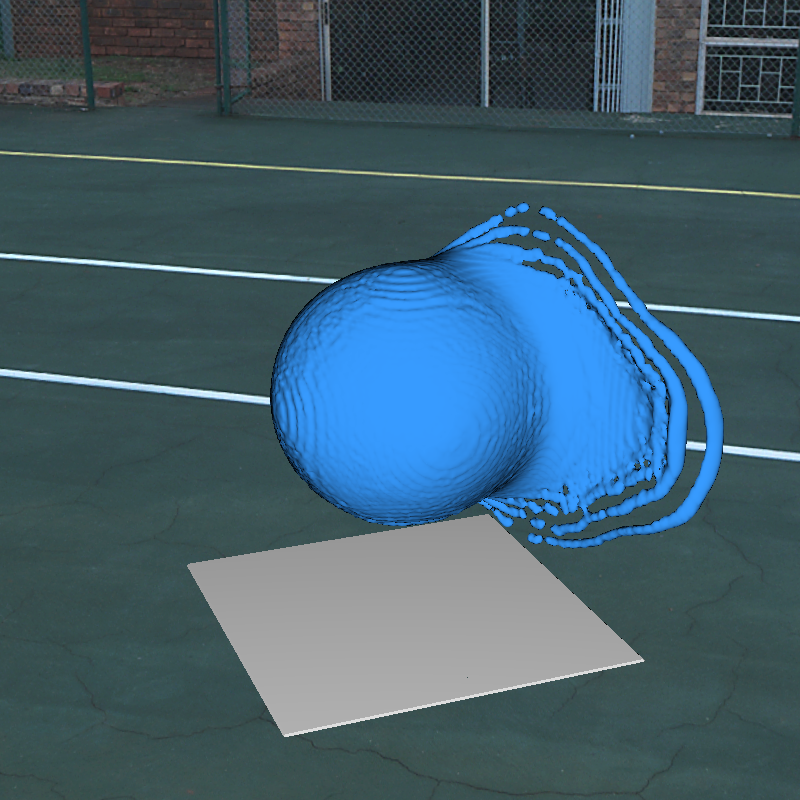
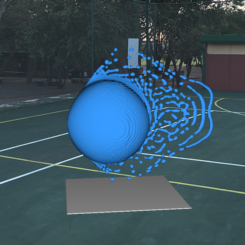
Figure 2: A selection of nine frames from the multi-view dataset presented in Section 4.2.2, from the duck, ship and droplets scenes (top to bottom).

Another very recent line of research is the application of the NeRF [MST^∗20] inverse rendering paradigm to fluid dynamics scenes. The first work to successfully regularize a 4D NeRF training with Navier-Stokes priors was published by Chu et al. [CLZ^∗22]; they introduced a training scheme where a density network and a velocity network optimize each other attempting to satisfy physical constraints. The result was a model that could be trained with very few camera views and correctly reconstructed smoke density fields. NeuroFluid [GDWY22] is closely related, as they obtained the same results with a Lagrangian perspective, by including differentiable physics constraints on particles in the volume rendering function used to optimize their model. Li et al. [LQC^∗23] proposed PAC-NeRF, a method combining the Eulerian and Lagrangian perspectives to obtain a general model with impressive performance on a vast selection of dramatically varying materials. All these methods assume that the fluid color may be “painted” upon its geometry such as a texture, ignoring the material properties which naturally occur in real world fluids. NeReF [WYC^∗22] studied a NeRF formulation taking into account reflective/transmissive materials, allowing to properly represent the interaction of light with fluids such as water.

A generalized issue among most of the work we cited in this section is the lack of a common benchmark dataset, which the authors addressed by generating new simulations datasets in order to evaluate their methods. Our generation tool solves this issue by allowing to a) export fluids both as particles and density fields b) export multi-view renderings of the simulation c) efficiently re-generate the dataset with just a configuration file, thus avoiding the need to share massive amounts of data.

3 Related work

Our work is by no means the first attempt at a structured collection of fluid simulation data; in this section, we discuss previous literature and point out the main differences with our contribution.

The Johns Hopkins Turbulence Databases [PBLM07, LPW^∗08] is a collection of massive volumetric databases of long, extremely high resolution turbulent flows, frequently expanded with new contributions [GKY^∗16]. Each database counts thousands of frames, with billions of voxels per frame: such scale and granularity makes the JHTD impractical for CG applications, in fact, the project is more oriented towards geophysical and engineering fluid dynamics (e.g.meteorology, hydraulics, aerodynamics).

Several datasets were published as secondary contributions of data-driven simulation papers. Pfaff et al.[PFSGB21] proposed a method to represent physical systems as triangle meshes, and learn how to solve various simulation tasks on the mesh domain via graph neural networks [SGT^∗08, VCC^∗17, KW16]. Their fluid environments, however, were limited to 2D coordinates, since planar meshes are not suited to represent 3D volumes. A similar discussion stands for the dataset presented in EAGLE [JBN^∗23], which is mesh-based and focused on turbulent wind dynamics when changing the shape of the simulation boundary. Stachenfeld et al.[SFK^∗22] introduced three volumetric datasets in one, two and three dimensions, computed from known chaotic PDEs arising in real-world settings. Our work’s focus is restricted to fluid dynamics and their applications in computer graphics, given the additional visual modality of our data. Finally, it is worth noting that, while the synthetic datasets used in Ummenhofer et al.[UPTK20] were presented as minor contributions, they were successively used for evaluation of similar methods such as [PUKT22].

The work most similar in spirit to ours is ScalarFlow [EUT19]. This is a collection of video captures of real-world smoke plumes dynamics (see Figure 1), coupled with density field reconstructions of the corresponding volumetric data computed by an algorithm proposed by the authors. While ScalarFlow is a large scale dataset (counting ca. 26 billion voxels of data), its scope is limited to the real-world capture setting set up by the authors; its distribution could easily be approximated within our generation framework without the additional cost of capture, in settings where using real data over synthetic would provide no significant advantage.

Lastly, we mention that the application of large scale simulation data for training and evaluation of data driven models is common for other physical simulation domains as well, such as garment animation. Two notable examples from this field are the datasets presented in CLOTH3D [BME20] and TailorNet [PLPM20].

4 Dataset

In this section, we discuss our data generation procedure, including high-level details of its implementation. For more in-depth documentation, we refer to our code release url-placeholder. The procedure is then applied to generate two medium-scale benchmark datasets for data-driven fluid simulation, as well as a collection of scenes for fluid inverse rendering algorithms.

4.1 Data generation

Our C++ code library is based on a refactoring of the FluidX3D Lattice-Boltzmann GPU simulator [Leh]. This particular simulator was chosen considering its a) impressive efficiency even on medium-range hardware b) efficient built-in ray-traced rendering features c) wide compatibility with several operating systems and GPU architectures, thanks to the OpenCL implementation of its kernels. We preserved the core implementation, while improving its API in order to conveniently expose most of its functionalities via a generic Scene class. These objects, which allow for both fine-grained configuration and inheritance to augment base behaviour, essentially represent the initial state and parameters of the simulation. For instance, the initial fluid shape and boundary conditions can be supplied as input mesh files which can be translated, rotated, and rescaled. Activating more specialized features (e.g.point-wise external force fields, inflows, outflows) requires overriding basic Scene functionalities.

Listing 1: JSON configuration file for our generation procedure. Variables are sampled and aggregated in order to generate configuration files for individual instances in the dataset. Fluid bodies and solid obstacles can be specified both as constants and variables, and sampled according to specific properties of geometric primitives or meshes (e.g.center, scale, rotation).

⬇

"export_root": "path/to/out/dir",

"seed": 123456,

"constants": {

"sim_params": {

"Nx": 256, "Ny": 256, "Nz": 256,

...

},

"obstacles": {

...

},

...

},

"variables": {

"sim_params": {

"nu": {

"type": "linscale",

"vmin": 0.0005, "vmax": 0.005, "steps": 20

},

"sigma": {

"type": "normal",

"mean": 0.001, "std": 0.0005, "nsamples": 20

}

},

"fluids": [

...

]

}

The refactored implementation is employed as a library in order to define dataset-specific Scene subclasses, which are accessed via an executable file allowing for their complete configuration through a simple json file. Given this backbone, the generation procedure was implemented as a simple Python script which generates configuration files and feeds them to the simulation tool. This script requires, besides global generation parameters (e.g.seed for reproducibility), a set of constants and a set of variables. The constants block is copied as-is to the generated instances, while variables are sampled according to their selected type (linear interval, uniform, normal, collection, and more complex structures). Additionally, a maximum number of scenes can be specified, in which case the scene instances are sampled uniformly from all the possible combinations of variables. All this information can be supplied to the generation script by a separate json file.

During simulation, specific frames can be extracted both as multi-view renderings and geometric information. For rendering, we exploit the ad-hoc algorithm implemented in FluidX3D, which sacrifices some measure of photorealism in favour of superior efficiency. In particular, camera rays are only bounced twice and no BDSF sampling is performed; this way, the light interactions of the water material we use for fluids can still be displayed, while the rendering procedure remains really fast, also due to it being run on the GPU (see Table 1). For geometric information extraction, we allow for two distinct modalities: the first one allows to export the fluid as a binary array of particles, where the number of exported particles is supplied as an input in the configuration file. Alternatively, the second modality allows to export the fluid’s density field as a 3D matrix stored in COO sparse format as a binary array. We find that this method is very memory-efficient (see Table 3), but selecting a specific number of particles may be more convenient when the simulation resolution is really high. We provide a Python loader to Numpy arrays for both file formats.

4.2 Data distribution

4.2.1 Any-scale datasets of dynamically close simulations

The first application we present for the procedure we described in Section 4.1 is devoted to the generation of collections of “semantically” (in a fluid dynamics sense) close simulations, regardless of the scale of such collections. To this end, we introduce two medium scale benchmark datasets based on well-known fluid dynamics settings. Throughout this section, we will refer to 3D coordinate systems assuming that the up-axis is the $z$ direction.

The first dataset, which we refer to as dam-break, is a collection of 200 simulations with 500 output frames each, one every 20 LBM simulation steps (for a total of 10k steps). In this setting, a cuboid of fluid is placed in contact with the lower face of a cubic boundary $B=(\mathbf{p},\mathbf{q})$, where $\mathbf{p}_{\{x,y,z\}}$ and $\mathbf{q}_{\{x,y,z\}}$ are the minimum/maximum coordinate values for the vertices of $B$, respectively. The scene is then simulated at resolution $\mathbf{N}=(256,256,256)$ under gravity, with no initial velocity. We set the viscosity $\nu=0.005$ and the surface tension $\sigma=0.0001$, which we find to result in physical properties similar to those of water for our simulator. The only variable for our scene generation procedure is the initial placement of the dam inside the scene: if we represent the cuboid by its center and sides, i.e., $D=(\mathbf{c},\mathbf{s})$, we set the $y$ coordinates to span the entire $y$-axis ($\mathbf{s}_{y}=\mathbf{q}_{y}-\mathbf{p}_{y},\mathbf{c}_{y}={\mathbf{s}_{y}}/{2}$) and sample the $x$ coordinates as

$$\mathbf{c}_{x} \sim\mathcal{U}\left(\left[\mathbf{p}_{x}+\delta_{x};\mathbf{q}_{x}-\delta_{x}\right]\right)$$ (1)

$$\mathbf{s}_{x} \sim\mathcal{U}\left(\left[k\dfrac{\mathbf{q}_{x}-\mathbf{p}_{x}}{\mathbf{N}_{x}};\min\{\mathbf{c}_{x},\mathbf{N}_{x}-\mathbf{c}_{x}\}\right]\right)$$ (2)

where we set $k$ and $\delta_{x}$ to the 10% and the 25% of $\mathbf{q}_{x}-\mathbf{p}_{x}$, respectively. For the $z$ coordinates, since we require the dam to touch the ground, we only sample the center

$$\mathbf{c}_{z}\sim\mathcal{U}\left(\left[\mathbf{p}_{z}+\delta_{z};\dfrac{\mathbf{q}_{z}-\mathbf{p}_{z}}{2}\right]\right)$$ (3)

and set $\mathbf{s}_{z}=2\mathbf{c}_{z}$, where $\delta_{z}$ is set to the 25% of $\mathbf{q}_{z}-\mathbf{p}_{z}$. We perform this sampling 200 times and simulate the resulting scenes, extracting visualizations from a single camera and particle geometry with 5000 particles. The final dataset counts 100.000 frames, totalling 42GB of memory.

The second dataset, named ball-drop, is a collection of 400 simulations with 250 output frames each, one every 20 LBM simulation steps (for a total of 5 steps). We consider the dynamics of a sphere of fluid falling inside a cubic boundary $B=(\mathbf{p},\mathbf{q})$ under the effects of gravity, with an initial velocity. We maintain the same resolution of the dam-break dataset and vary the viscosity and surface tension to represent different material properties. Setting $\nu=0.0005$ and $\sigma=0.01$ yields a fluid with properties similar to those of mercury. To generate scenes, we need to sample both the initial shape of the fluid and the velocity at $t=0$. We represent spheres as their center and radius, i.e., $S=(\mathbf{c},r)$, and we fix $\mathbf{c}_{y}$ to the 50% of $\mathbf{q}_{y}-\mathbf{p}_{y}$ in order to reduce rotationally-equivalent simulations. For the same reason, we sample most of the magnitude of the initial velocity vector $\mathbf{v}$ into its $y$ coordinate: $\mathbf{v}_{i}\sim\mathcal{N}\left(\mathbf{m}_{i},\mathbf{s}_{i}\right)$, where $\mathbf{m}=(0.0,0.1,0.0),\mathbf{s}=(0.02,0.02,0.02)$. On the other hand, the radius and remaining center coordinates are sampled uniformly, as for the dam-break dataset:

$$\mathbf{c}_{x} \sim\mathcal{U}\left(\left[\mathbf{p}_{x}+\epsilon;\mathbf{q}_{x}-\epsilon\right]\right)$$ (4)

$$\mathbf{c}_{z} \sim\mathcal{U}\left(\left[\mathbf{p}_{z}+\epsilon;\mathbf{q}_{z}-\epsilon\right]\right)$$ (5)

$$r \sim\mathcal{U}\left(\left[\mu;\eta\right]\right)$$ (6)

where we set $\mu$ and $\epsilon$ to the 10% and the 25% of $\mathbf{q}_{x}-\mathbf{p}_{x}$, respectively, and $\eta=\min\{\min\{\mathbf{c}_{x},\mathbf{N}_{x}-\mathbf{c}_{x}\},\min\{\mathbf{c}_{z},\mathbf{N}_{z}-\mathbf{c}_{z}\}\}$ is the smallest distance from the sampled center to the bounding box. This selection allows to sample the initial fluid configuration completely inside the given bounding box. We sample a total of 400 such scenes by combining these variables, extracting visualizations from a single camera and particle geometry with 3000 particles. As for dam-break, the dataset counts 100.000 frames, but only amounts to 27GB of memory since less particles are saved to disk, due to the inferior volume of fluids in this dataset’s scenes.

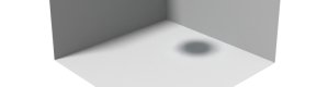
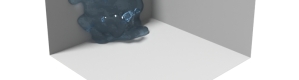
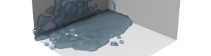
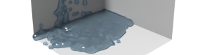
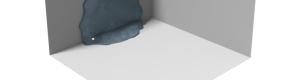
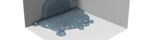
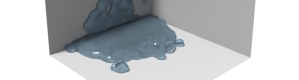
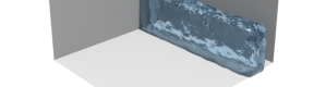
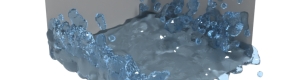
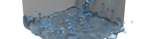
\begin{overpic}[width=108.405pt,trim=0.0pt 56.9055pt 0.0pt 156.49014pt,clip]{resources//imgs//dam-break-comparison//gt/canyon_rotate_0000.jpg} \put(45.0,-12.5){{0.0s}} \put(145.0,-12.5){{1.2s}} \put(245.0,-12.5){{2.4s}} \put(345.0,-12.5){{3.6s}} \par\put(0.0,15.0){\rotatebox{90.0}{{Ground truth}}} \put(0.0,90.0){\rotatebox{90.0}{{DLF~{}\cite[cite]{[\@@bibref{}{Ummenhofer2020Lagrangian}{}{}]}}}} \put(0.0,165.0){\rotatebox{90.0}{{Ground truth}}} \put(0.0,240.0){\rotatebox{90.0}{{DLF~{}\cite[cite]{[\@@bibref{}{Ummenhofer2020Lagrangian}{}{}]}}}} \end{overpic}

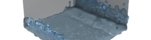
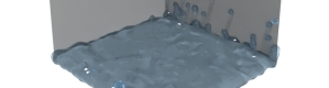
Figure 3: Samples extracted from 300 frames rollouts of two separate Deep Lagrangian Fluids models trained on our dam-break and ball-drop datasets, with unseen initial conditions. First two rows show, respectively, the ground truth and the output of the model for a test-set ball drop scene. The last two rows analogously show the ground truth and result for a test-set dam break scene.

4.2.2 Hand-crafted multi-view scenes

Secondarily, we applied our generation procedure to simulate a small collection of interesting hand-crafted scenes, whose main application is intended as a particularly complex benchmark set for inverse rendering and surface recovery algorithms.

This small dataset counts 5 scenes, each simulated for 4500 LBM steps, of which one every 30 is rendered with resolution $800\times 800$, from 10 different random viewpoints in the upper hemisphere, and exported as a particle array, for a total of 150 frames exported (or 5 seconds of data at 30 fps). We render each scene twice, using both a blue Lambertian material and a realistic water-like material for the fluid. For each camera, a fluid-less render is also produced (only showing the background) and the camera parameters are exported as a json file, composed by the two matrices

$$K=\begin{pmatrix}f_{x}&0&c_{x}\\ 0&f_{y}&c_{y}\\ 0&0&0\\ \end{pmatrix}$$ (7)

$$Rt=\begin{pmatrix}r_{xx}&r_{xy}&r_{xz}&t_{x}\\ r_{yx}&r_{yy}&r_{yz}&t_{y}\\ r_{zx}&r_{zy}&r_{zz}&t_{z}\\ \end{pmatrix}$$ (8)

The data totals 8.8GB.

The scenes are not intended to span a vast range of fluid behaviours, but they can be viewed as increasingly complex cases against which to evaluate novel methods. The ball and duck scenes are simple gravity simulations, with different material properties (they differ in viscosity and surface tension) and with both very simple and slightly more interesting initial geometry. The dam scene is a classic dam break similar to the ones discussed in Section 4.2.1. The ship scene portraits a complex interaction between a dam of fluid subject to an initial velocity and a static obstacle in the shape of a small boat. Lastly, the droplets scene showcases a the simulation of two spheres of fluid in a vacuum subject to a point-wise external force field. We show a selection frames from the presented dataset in Figure 2.

4.2.3 Copyright information

Along with our dataset, we redistribute a small set of meshes and HDRI environment textures which we used to make our datasets more interesting. All such content was obtained from polyhaven.com under CC-0 copyright license (no rights reserved). We gratefully acknowledge the authors of employed assets in Section 6.

5 Evaluation

5.1 Examples of applications

5.1.1 Data-driven Fluid Simulation

In this section, we test the suitability of the benchmark datasets described in Section 4.2.1 to train a data-driven model.

Model

[UPTK20] aims to understand fluid mechanics by studying particle motion. In particular, a continuous convolutional network is fed with a collection of particles, each paired with its features. Each particle is associated with a feature vector that is a constant scalar of 1, paired with the particle’s velocity, denoted by $\mathbf{v}$, and its viscosity, $\nu$. Therefore, at any timestep $n$, a particle $p_{i}^{n}$ is represented by the tuple $\left(\mathbf{x}_{i}^{n},\left[1,\mathbf{v}_{i}^{n},\nu_{i}\right]\right)$. To compute the intermediate velocities and positions and integrate external force information for the network, the velocity is listed as an input feature. Using Heun’s method, the intermediate velocities $\mathbf{v}_{i}^{n*}$ and positions $\mathbf{x}_{i}^{n*}$ commencing from timestep $n$ are then computed as:

$$\mathbf{v}_{i}^{n*}=\mathbf{v}_{i}^{n}+\Delta t\mathbf{a}_{\mathrm{ext}}$$ (9)

$$\mathbf{x}_{i}^{n*}=\mathbf{x}_{i}^{n}+\Delta t\frac{\mathbf{v}_{i}^{n}+\mathbf{v}_{i}^{n*}}{2}$$ (10)

where $\mathbf{a}_{\text{ext }}$ represents an acceleration vector, enabling the application of external forces like fluid control or gravity. These intermediate values are devoid of any particle or scene interactions; such interactions are incorporated using the ConvNet. For the network to manage collisions, another group of static particles $s_{j}$ are introduced. These are sampled along scene boundaries and paired with normals $\mathbf{n}_{j}$ as their feature vectors, expressed as $s_{j}=\left(\mathbf{x}_{j},\left[\mathbf{n}_{j}\right]\right)$. The network performs the function:

$$\left[\Delta\mathbf{x}_{1},\ldots,\Delta\mathbf{x}_{N}\right]=\operatorname{ConvNet}\left(\left\{p_{1}^{n*},\ldots,p_{N}^{n*}\right\},\left\{s_{1},\ldots,s_{M}\right\}\right),$$

employing convolutions to merge features from both sets of particles. Here, $\Delta\mathrm{x}$ serves as a position correction, factoring in all particle interactions, including collisions with the scene. The correction is finally used to update positions and velocities for timestep $n+1$ with:

$$\mathbf{x}_{i}^{n+1} =\mathbf{x}_{i}^{n*}+\Delta\mathbf{x}_{i}$$ (11)

$$\mathbf{v}_{i}^{n+1} =\frac{\mathbf{x}_{i}^{n+1}-\mathbf{x}_{i}^{n}}{\Delta t}.$$ (12)

We will refer to this model as Deep Lagrangian Fluids (DLF).

Experiment and results

We train DLF separately over both dam-break and ball-drop, split as train and validation sets with a 90:10 ratio. Consisting of $200$ and $400$ simulations each, the train datasets consist of $180$ and $360$ simulations for ball-drop and dam-break respectively. Having $500$ and $250$ frames per simulation, the total number of frames amounts to $100.000$ for both datasets. Figure 3 shows a qualitative comparison of the model prediction versus the ground truth simulation, after training DLF to convergence (50.000 total iterations) on both dam-break and ball-drop. Remarkably, the model is able to consistently predict a realistic behaviour throughout the simulation, proving the data to be suitable to be used in data-driven pipelines. As showed in the picture, the model succeeds to learn visually appealing solutions in both settings, up to evident mistakes in localized regions of space. Since the surface tension is not made explicit to the model, the optimization process attempts to learn a simulator which satisfies the data prior as well as possible, resulting in some imprecision for cases where the fluid behaviour is particularly influenced by surface tension (e.g.third and fourth frame of the first row, Figure 3).

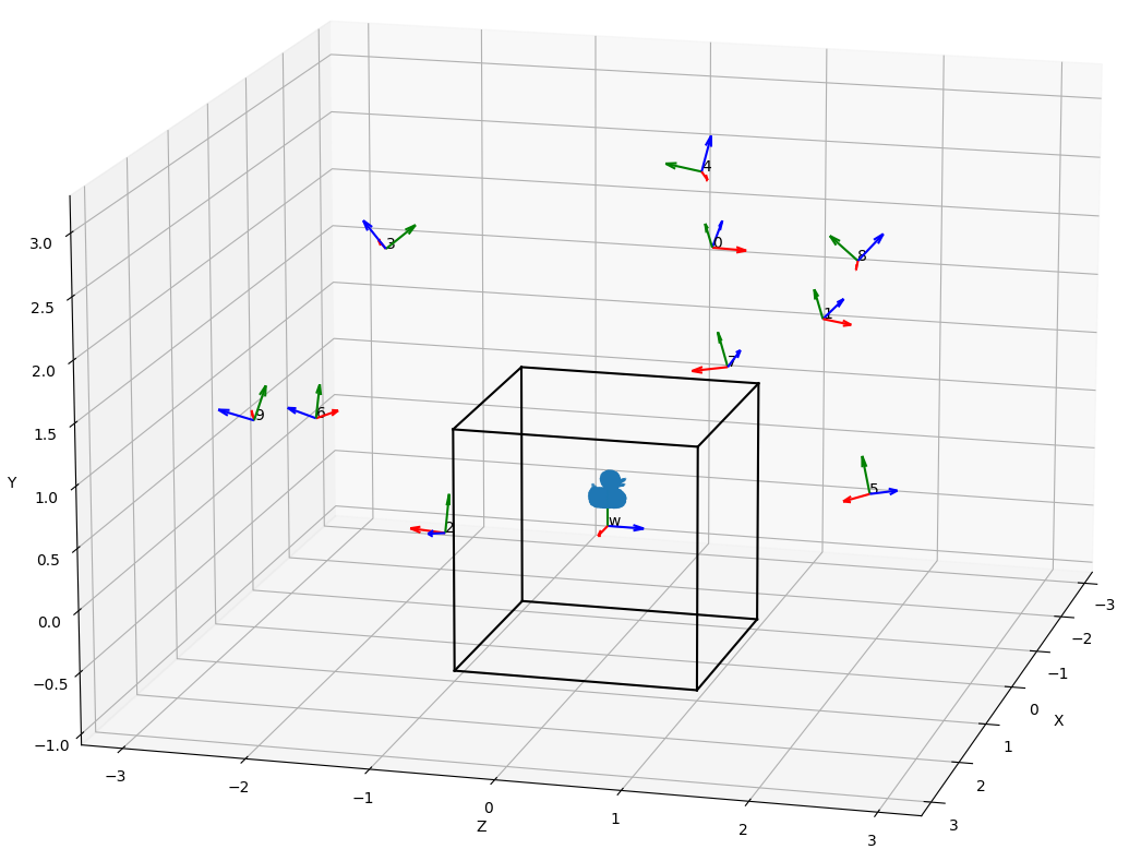
Figure 4: Randomly sampled camera poses and simulation-generated particles for the first frame of the duck scene.

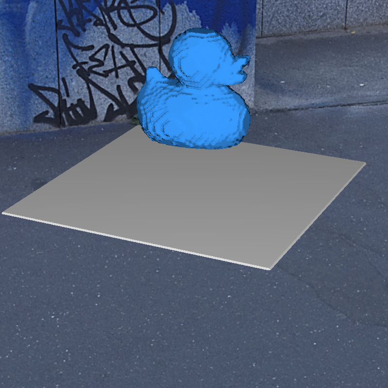
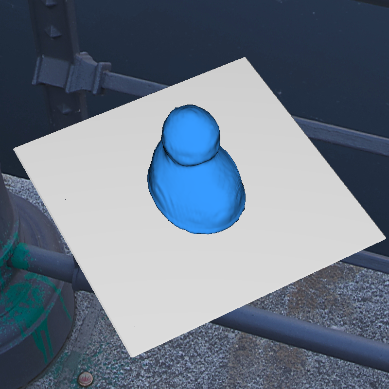
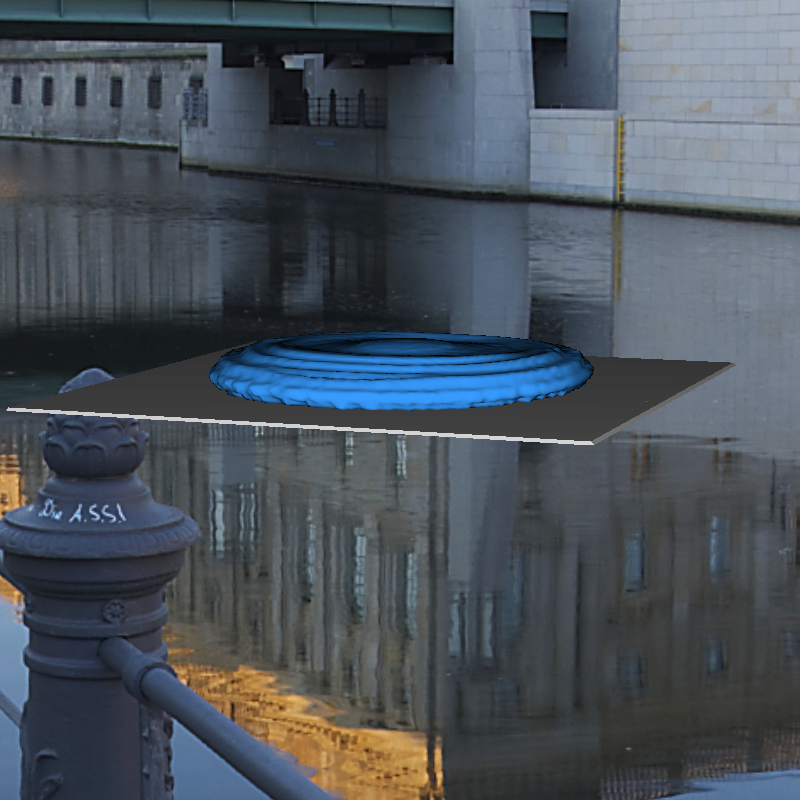
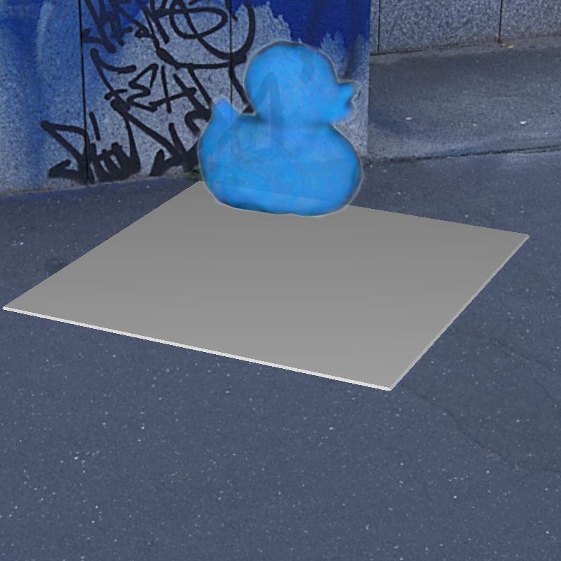
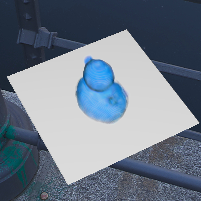
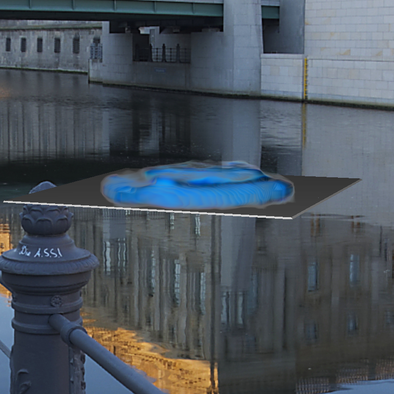
Figure 5: Top: a subset of the views in our duck scene training data. Bottom: PAC-NeRF [LQC^∗23] reconstruction and rendering for the same (unseen) views (the background is not learned by the model, so it was manually composited for this visualization).

5.1.2 Inverse Rendering of Fluid Dynamics Scenes

Our method allows the generation of multi-view video data for the inverse rendering task composed of image-pose pairs over time. By defining a $\Delta t$ and a set of randomly sampled cameras on the upper hemisphere 4, we render the scene from such viewpoints during the simulation. While our data could be used to train several NeRF-based models, whether static or dynamic, we tested them on PAC-NeRF [LQC^∗23], which aims to recover an explicit geometric representation and physical properties of the dynamic object of interest in a scene. It does so blending neural scene representations and explicit differentiable physics engines for continuum materials.

A dynamic NeRF comprises time-dependent volume density field $\sigma(\mathbf{x},t)$ and a time-and-view-dependent appearance (color) field $\mathbf{c}(\mathbf{x},\omega,t)$ for each point $\mathbf{x}\in\mathbb{R}^{3}$, and directions $\omega=(\theta,\phi)\in\mathbb{S}^{2}$ (spherical coordinates). The appearance $\mathbf{C}(\mathbf{r},t)$ of a pixel specified by ray direction $\mathbf{C}(\mathbf{r},t)$ $\left(s\in\left[s_{\min},s_{\max}\right]\right)$ is obtained by differentiable volume rendering [MST^∗20]:

$$\mathbf{C}(\mathbf{r},t)=\int_{s_{n}}^{s_{f}}T(s,t)\sigma(\mathbf{r}(s),t)\mathbf{c}(\mathbf{r}(s),\omega,t)ds+\mathbf{c}_{bg}T\left(s_{f},t\right)$$ (13)

$$T(s,t)=\exp\left(-\int_{s_{n}}^{s}\sigma(\mathbf{r}(\bar{s}),t)d\bar{s}\right)$$ (14)

The dynamic NeRF can therefore be trained to minimize the rendering loss:

$$\mathcal{L}_{\text{render }}=\frac{1}{N}\sum_{i=0}^{N-1}\frac{1}{|\mathcal{R}|}\sum_{\mathbf{r}\in\mathcal{R}}\left\|\mathbf{C}\left(\mathbf{r},t_{i}\right)-\hat{\mathbf{C}}\left(\mathbf{r},t_{i}\right)\right\|^{2}$$ (15)

where $N$ is the number of frames of videos, $\hat{\mathbf{C}}\left(\mathbf{r},t_{i}\right)$ is the ground truth color observation.

PAC-NeRF first initializes an Eulerian voxel field over the first frame of the sequence. It then uses a grid-to-particle conversion method to obtain a Lagrangian particle field; this is advected, enforcing that the appearance and volume density fields admit conservation laws characterized by the velocity field $\mathbf{v}$ of the underlying physical system:

$$\frac{D\sigma}{Dt}=0,\quad\frac{D\mathbf{c}}{Dt}=0$$ (16)

with $\frac{D\phi}{Dt}=\frac{\partial\phi}{\partial t}+\mathbf{v}\cdot\nabla\phi$ being the material derivative of an arbitrary time-dependent field $\phi(\mathbf{x},t)$. Moreover, the velocity field must obey momentum conservation for continuum materials:

$$\rho\frac{D\mathbf{v}}{Dt}=\nabla\cdot\boldsymbol{T}+\rho\mathbf{g}$$ (17)

where $\rho$ is the physical density field, $\boldsymbol{T}$ is the internal Cauchy stress tensor, and $\mathbf{g}$ is the acceleration due to gravity and it is evolved using a differentiable Material Point Method (MPM) [HFG^∗18]. The advected field is then mapped back to the Eulerian domain using the particle-to-grid conversion and is used for collision handling and neural rendering. We refer to the original paper for more technical details.

Table 1: Resource consumption in terms of CPU memory, GPU memory, scene size and time for various rendering resolutions. The simulation resolution is set to $256^{3}$, while the number of LBM steps is set to $4500$, with one every 30 steps being exported as output frame. The number of rendering views is set to $1$. FHD, 2K and 4K refer to resolutions (1920, 1080), (2560, 1440), (3840, 1920) respectively. Values are averaged for repeated runs over 5 scenes.

Rendering resolutions	$800\times 800$	FHD	2K	4K
Memory (CPU)	374.4	374.4	374.4	374.4
Memory (GPU)	1242.4	1244.4	1246.4	1248.4
Scene size (MB)	780.35	861.44	912.94	983.42
Time (s)	16.97	20.46	21.13	22.48

Table 2: Throughput for generation of the dam-break and ball-drop datasets. Even assuming some degradation of performance (i.e.ca. 10 FPS), our method can generate a large scale dataset with 1 million frames (ca. $16\cdot 10^{12}$ voxels, assuming the same resolution of presented datasets) in little more than 24 hours.

Dataset	Frame count	Generation time (s)	Throughput (FPS)
dam-break	100.000	7618	13.12
ball-drop	100.000	7353	13.59

Experiment and results

We trained PAC-NeRF on duck by subsampling a 1-second simulation of 1800 frames down to 13 frames with a $\Delta t$ of $\approx 0.077s$. As visually shown in 5 the model can produce faithful renders of the simulation proving that our multi-view data generation is suitable to be used in methods using inverse rendering in the domain of fluid dynamic scenes. PAC-NeRF imposes far more advection-related constraints on the NeRF model being learned than other 4D NeRF methods; this allows the identification of the dynamics of the scene and leads to the beneficial side-effect of producing smooth and plausible inter-frame reconstructions. However, this often leads the quality of supervised frame reconstruction to degrade over time, as shown in 6, whereas any other method for 4D NeRF would have kept these values stable, at the cost of non physically plausible interpolations between supervised simulation steps.

5.2 Generation performance

Now we evaluate the efficiency of our generation procedure. By leveraging a GPU implementation, we show that our method is fast enough to bypass the need for sharing data, as the json configuration is all you need to recreate an exact copy of a dataset in a reasonable amount of time using our generation tool.

Table 3: Resource consumption in terms of CPU memory, GPU memory, scene size and time for various simulation resolutions. The number of LBM steps is set to $4500$, with one every 30 steps being exported as output frame. No rendering is performed to discard its impact on the computational cost. Values are averaged for repeated runs over 5 scenes.

Simulation resolutions	$64^{3}$	$128^{3}$	$256^{3}$	$512^{3}$
Memory (CPU)	5.6	46.8	374.4	2995.2
Memory (GPU)	148.6	270.8	1242.4	9015.2
Scene size (MB)	11.12	83.12	653.2	4110.02
Time (s)	5.59	7.82	16.05	112.8

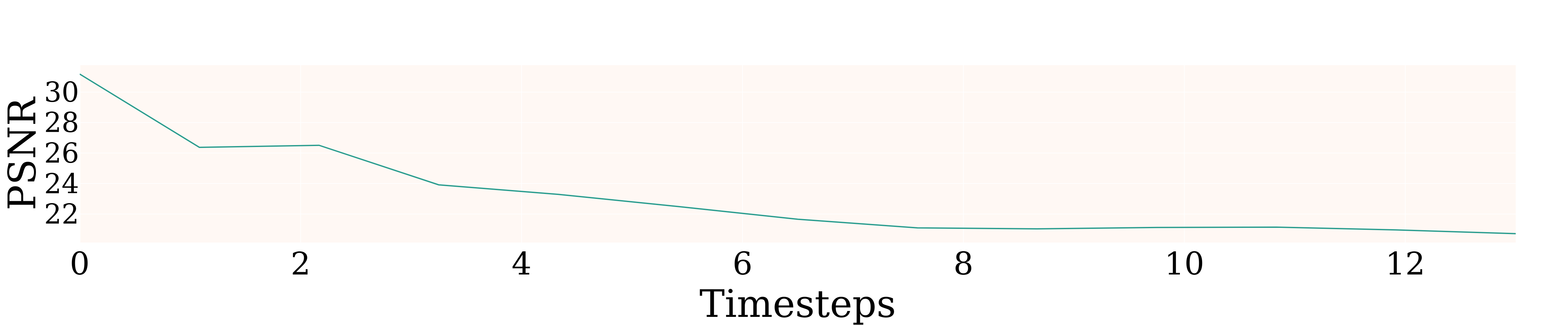
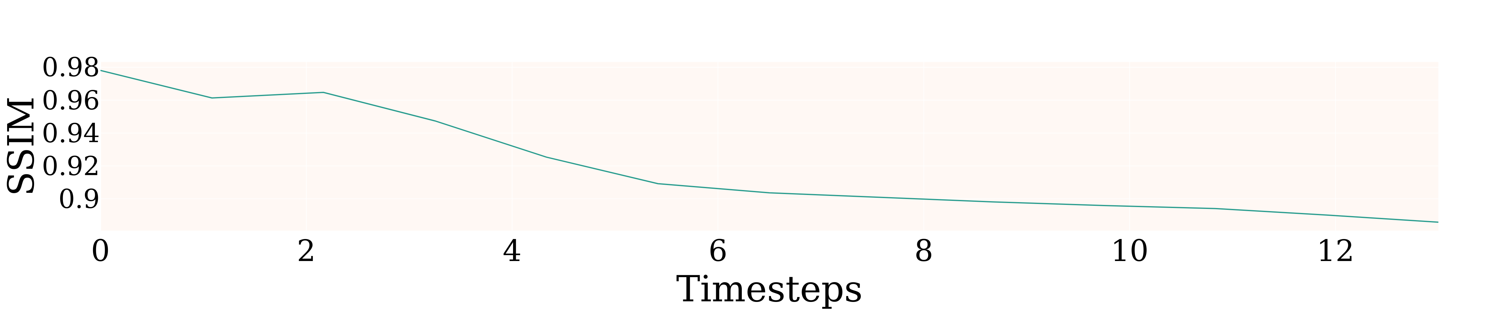
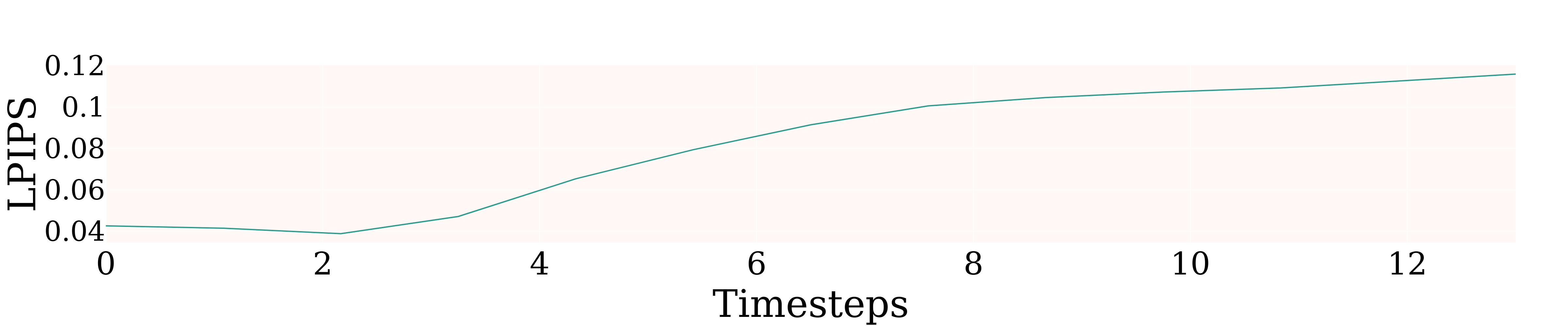
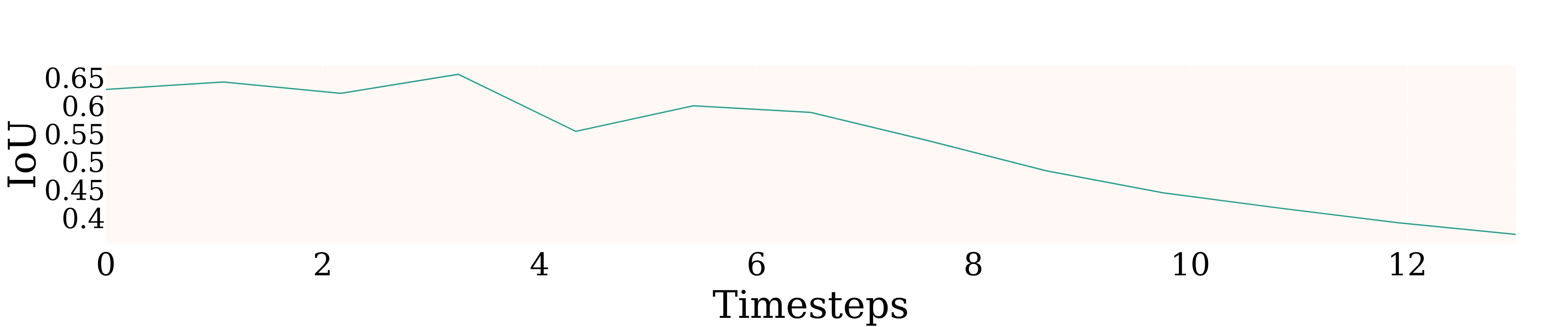
Figure 6: PAC-NeRF evaluation on duck. Both rendering quality and IoU over occupancy grids degrade as the simulation progresses because the neural radiance field reconstruction gets increasingly constrained by the physics-based losses. Note that the image metrics are computed only on the masked foreground object.

Our dam-break and ball-drop datasets, both totalling 100.000 frames, were generated at a simulation resolution of $256^{3}$, with a single rendered camera per simulation at low resolution ($800\times 800$), to offer a visual support to the generated data. As we report in Table 2, we reach a throughput of ca. 13 frames per second, allowing to generate 100.000 frames of data in a little more than two hours. We further analyze our generation procedure’s runtime and memory occupancy by collecting performance data over multiple runs, changing the simulation resolution and the rendering resolution. The results can be appreciated in Table 3 and Table 1, respectively: exploiting GPU programming massively benefits both the simulation and rendering steps, so much so that rendering 150 frames even in 4K only accounts for 28% of the total computation time. Furthermore, Table 3 shows the convenience in our sparse format for storing density fields: while 4GB per scene can seem to be a lot at simulation resolution $512$, the dense version would have required ca. 80GB per scene ($150\cdot 512^{3}$ floats), i.e., we only require 5% of the disk memory.

All generations were run on medium/high-end consumer hardware, to further solidify the claim that our data can be re-generated locally, without the need for sharing entire datasets. Our machine runs Windows 11 over 32GB of DDR4 RAM, an intel core i7 12700K CPU (3.6GHz, 12 physical processors, 20 logical processors), and a NVIDIA RTX4070Ti GPU (7680 CUDA cores). The data was generated on an SSD drive to minimize disk latency.

6 Conclusions

Our work proposes an efficient generation procedure for multimodal fluid simulation data and three benchmark datasets for future research. We describe the generation process for these datasets and the interface to the software tool. Furthermore, we evaluate its performance, which resulted in an impressive 13FPS throughput, which enables generating large scale datasets on consumer-grade hardware within reasonable time scales. We claim our proposal to be a valuable tool for the community, and we validate this by employing our three generated datasets to train models for data-driven fluid simulation and fluid inverse rendering, respectively.

6.1 Acknowledgements

The work of artists Rico Cilliers, Plat251, Alexander Scholten, Andreas Mischok, Sergej Majboroda, Dimitrios Savva and Jarod Guest was employed in our project to create interesting scene via through complex fluid shapes, boundary conditions and HDRI maps. We wish to thank them for sharing their work on Polyhaven, free of any copyright license.

References

- [BLDL20] Bai K., Li W., Desbrun M., Liu X.: Dynamic upsampling of smoke through dictionary-based learning. ACM Trans. Graph. 40, 1 (sep 2020). URL: https://doi.org/10.1145/3412360, doi:10.1145/3412360.
- [BME20] Bertiche H., Madadi M., Escalera S.: Cloth3d: clothed 3d humans. In European Conference on Computer Vision (2020), Springer, pp. 344–359.
- [BRPMB17] Bogo F., Romero J., Pons-Moll G., Black M. J.: Dynamic FAUST: Registering human bodies in motion. In IEEE Conf. on Computer Vision and Pattern Recognition (CVPR) (July 2017).
- [BWDL21] Bai K., Wang C., Desbrun M., Liu X.: Predicting high-resolution turbulence details in space and time. ACM Trans. Graph. 40, 6 (dec 2021). URL: https://doi.org/10.1145/3478513.3480492, doi:10.1145/3478513.3480492.
- [CLZ∗22] Chu M., Liu L., Zheng Q., Franz E., Seidel H.-P., Theobalt C., Zayer R.: Physics informed neural fields for smoke reconstruction with sparse data. ACM Transactions on Graphics 41, 4 (aug 2022), 119:1–119:14.
- [EUT19] Eckert M.-L., Um K., Thuerey N.: Scalarflow: A large-scale volumetric data set of real-world scalar transport flows for computer animation and machine learning. ACM Trans. Graph. 38, 6 (nov 2019). URL: https://doi.org/10.1145/3355089.3356545, doi:10.1145/3355089.3356545.
- [FSD∗20] Ferdian E., Suinesiaputra A., Dubowitz D. J., Zhao D., Wang A., Cowan B., Young A. A.: 4dflownet: Super-resolution 4d flow mri using deep learning and computational fluid dynamics. Frontiers in Physics 8 (2020). URL: https://www.frontiersin.org/articles/10.3389/fphy.2020.00138, doi:10.3389/fphy.2020.00138.
- [GDWY22] Guan S., Deng H., Wang Y., Yang X.: Neurofluid: Fluid dynamics grounding with particle-driven neural radiance fields. In ICML (2022).
- [GKY∗16] Graham J., Kanov K., Yang X. I. A., Lee M., Malaya N., Lalescu C. C., Burns R., Eyink G., Szalay A., Moser R. D., Meneveau C.: A web services accessible database of turbulent channel flow and its use for testing a new integral wall model for les. Journal of Turbulence 17, 2 (2016), 181–215. URL: https://doi.org/10.1080/14685248.2015.1088656, arXiv:https://doi.org/10.1080/14685248.2015.1088656, doi:10.1080/14685248.2015.1088656.
- [GSW21] Gao H., Sun L., Wang J.-X.: Super-resolution and denoising of fluid flow using physics-informed convolutional neural networks without high-resolution labels. Physics of Fluids 33, 7 (2021).
- [HFG∗18] Hu Y., Fang Y., Ge Z., Qu Z., Zhu Y., Pradhana A., Jiang C.: A moving least squares material point method with displacement discontinuity and two-way rigid body coupling. ACM Transactions on Graphics 37, 4 (2018), 150.
- [HHL∗05] Hoyer K., Holzner M., Lüthi B., Guala M., Liberzon A., Kinzelbach W.: 3d scanning particle tracking velocimetry. Experiments in Fluids 39 (2005), 923–934.
- [JBN∗23] JANNY S., Bénéteau A., Nadri M., Digne J., THOME N., Wolf C.: EAGLE: Large-scale learning of turbulent fluid dynamics with mesh transformers. In The Eleventh International Conference on Learning Representations (2023). URL: https://openreview.net/forum?id=mfIX4QpsARJ.
- [KAT∗19] Kim B., Azevedo V. C., Thuerey N., Kim T., Gross M., Solenthaler B.: Deep fluids: A generative network for parameterized fluid simulations. Computer Graphics Forum 38, 2 (2019), 59–70. URL: https://onlinelibrary.wiley.com/doi/abs/10.1111/cgf.13619, arXiv:https://onlinelibrary.wiley.com/doi/pdf/10.1111/cgf.13619, doi:https://doi.org/10.1111/cgf.13619.
- [KW16] Kipf T. N., Welling M.: Semi-supervised classification with graph convolutional networks. In International Conference on Learning Representations (2016).
- [Leh] Lehmann M.: Fluidx3d. URL: https://github.com/ProjectPhysX/FluidX3D.
- [LF22] Li Z., Farimani A. B.: Graph neural network-accelerated lagrangian fluid simulation. Computers & Graphics 103 (2022), 201–211.
- [LM22] Li M., McComb C.: Using physics-informed generative adversarial networks to perform super-resolution for multiphase fluid simulations. Journal of Computing and Information Science in Engineering 22, 4 (2022), 044501.
- [LMR∗15] Loper M., Mahmood N., Romero J., Pons-Moll G., Black M. J.: SMPL: A skinned multi-person linear model. ACM Trans. Graphics (Proc. SIGGRAPH Asia) 34, 6 (Oct. 2015), 248:1–248:16.
- [LPW∗08] Li Y., Perlman E., Wan M., Yang Y., Meneveau C., Burns R., Chen S., Szalay A., Eyink G.: A public turbulence database cluster and applications to study lagrangian evolution of velocity increments in turbulence. Journal of Turbulence 9, 31 (2008).
- [LQC∗23] Li X., Qiao Y.-L., Chen P. Y., Jatavallabhula K. M., Lin M., Jiang C., Gan C.: PAC-neRF: Physics augmented continuum neural radiance fields for geometry-agnostic system identification. In The Eleventh International Conference on Learning Representations (2023). URL: https://openreview.net/forum?id=tVkrbkz42vc.
- [MST∗20] Mildenhall B., Srinivasan P. P., Tancik M., Barron J. T., Ramamoorthi R., Ng R.: Nerf: Representing scenes as neural radiance fields for view synthesis. In ECCV (2020).
- [PBLM07] Perlman E., Burns R., Li Y., Meneveau C.: Data exploration of turbulence simulations using a database cluster. In SC ’07: Proceedings of the 2007 ACM/IEEE Conference on Supercomputing (2007), Association for Computing Machinery.
- [PFSGB21] Pfaff T., Fortunato M., Sanchez-Gonzalez A., Battaglia P.: Learning mesh-based simulation with graph networks. In International Conference on Learning Representations (2021). URL: https://openreview.net/forum?id=roNqYL0_XP.
- [PLPM20] Patel C., Liao Z., Pons-Moll G.: Tailornet: Predicting clothing in 3d as a function of human pose, shape and garment style. In IEEE Conference on Computer Vision and Pattern Recognition (CVPR) (jun 2020), IEEE.
- [PUKT22] Prantl L., Ummenhofer B., Koltun V., Thuerey N.: Guaranteed conservation of momentum for learning particle-based fluid dynamics. In Conference on Neural Information Processing Systems (2022).
- [SFK∗22] Stachenfeld K., Fielding D. B., Kochkov D., Cranmer M., Pfaff T., Godwin J., Cui C., Ho S., Battaglia P., Sanchez-Gonzalez A.: Learned simulators for turbulence. In International Conference on Learning Representations (2022). URL: https://openreview.net/forum?id=msRBojTz-Nh.
- [SGT∗08] Scarselli F., Gori M., Tsoi A. C., Hagenbuchner M., Monfardini G.: The graph neural network model. IEEE transactions on neural networks 20, 1 (2008), 61–80.
- [UPTK20] Ummenhofer B., Prantl L., Thuerey N., Koltun V.: Lagrangian fluid simulation with continuous convolutions. In International Conference on Learning Representations (2020).
- [VB22] Vinuesa R., Brunton S. L.: Enhancing computational fluid dynamics with machine learning. Nature Computational Science 2, 6 (2022), 358–366.
- [VCC∗17] Veličković P., Cucurull G., Casanova A., Romero A., Lio P., Bengio Y.: Graph attention networks. arXiv preprint arXiv:1710.10903 (2017).
- [WBT19] Wiewel S., Becher M., Thuerey N.: Latent space physics: Towards learning the temporal evolution of fluid flow. In Computer graphics forum (2019), vol. 38, Wiley Online Library, pp. 71–82.
- [WKA∗20] Wiewel S., Kim B., Azevedo V., Solenthaler B., Thuerey N.: Latent space subdivision: Stable and controllable time predictions for fluid flow (2020). arXiv preprint arXiv:2003.08723 (2020).
- [WXCT19] Werhahn M., Xie Y., Chu M., Thuerey N.: A multi-pass gan for fluid flow super-resolution. Proc. ACM Comput. Graph. Interact. Tech. 2, 2 (jul 2019). URL: https://doi.org/10.1145/3340251, doi:10.1145/3340251.
- [WYC∗22] Wang Z., Yang W., Cao J., Xu L., ming Yu J., Yu J.: Neref: Neural refractive field for fluid surface reconstruction and implicit representation. ArXiv abs/2203.04130 (2022). URL: https://api.semanticscholar.org/CorpusID:247315295.
- [XFCT18] Xie Y., Franz E., Chu M., Thuerey N.: tempogan: A temporally coherent, volumetric gan for super-resolution fluid flow. ACM Transactions on Graphics (TOG) 37, 4 (2018), 95.