Efficient Parallelization of a Ubiquitous Sequential Computation

Abstract

We find a succinct expression for computing the sequence $x_{t}=a_{t}x_{t-1}+b_{t}$ in parallel with two prefix sums, given $t=(1,2,\dots,n)$, $a_{t}\in\mathbb{R}^{n}$, $b_{t}\in\mathbb{R}^{n}$, and initial value $x_{0}\in\mathbb{R}$. On $n$ parallel processors, the computation of $n$ elements incurs $\mathcal{O}(\log n)$ time and $\mathcal{O}(n)$ space. Sequences of this form are ubiquitous in science and engineering, making efficient parallelization useful for a vast number of applications. We implement our expression in software, test it on parallel hardware, and verify that it executes faster than sequential computation by a factor of $\frac{n}{\log n}$.

1 Summary

Sequences of the form $x_{t}=a_{t}x_{t-1}+b_{t}$ are ubiquitous in science and engineering. For example, in the natural sciences, such sequences can model quantities or populations that decay or grow by a varying rate $a_{t}>0$ between net inflows or outflows $b_{t}$ at each time step $t$. In economics, such sequences can model investments that earn a different rate of return $a_{t}=(1+r_{t})$ between net deposits or withdrawals $b_{t}$ over each time period $t$. In engineering applications, such sequences are often low-level components of larger models, e.g., linearized recurrent neural networks whose layers decay token features in a sequence of tokens.

Given a finite sequence $x_{t}=a_{t}x_{t-1}+b_{t}$ with $n$ steps, $t=(1,2,\dots,n)$, where $a_{t}\in\mathbb{R}^{n}$, $b_{t}\in\mathbb{R}^{n}$, and initial value $x_{0}\in\mathbb{R}$, it’s not immediately obvious how one would compute all elements in parallel, because each element is a non-associative transformation of the previous one. In practice, we routinely see software code that computes sequences of this form one element at a time.

The vector $\log x_{t}$ is computable as a composition of two cumulative, or prefix, sums, each of which is parallelizable:

$$\log x_{t}=a^{*}_{t}+\log\left(x_{0}+b^{*}_{t}\right)\\$$ (1)

where $a^{*}_{t}$ and $b^{*}_{t}$ are the two prefix sums:

$$a^{*}_{t} =\overset{\text{{cum}}}{\sum\limits_{t}}\log a_{t}$$ (2)

$$b^{*}_{t} =\overset{\text{{cum}}}{\sum\limits_{t}}e^{\log b_{t}-a^{*}_{t}}.$$

The operator $\overset{\text{{cum}}}{\sum}$ computes a vector whose elements are a prefix sum, i.e., a cumulative sum.

We obtain $x_{t}$ with elementwise exponentiation:

$$x_{t}=e^{a^{*}_{t}+\log(x_{0}+b^{*}_{t})}.\\$$ (3)

Prefix sums are associative, making it possible to compute them by parts in parallel. Well-known parallel algorithms for efficiently computing the prefix sum of a sequence with $n$ elements incur $\mathcal{O}(\log n)$ time and $\mathcal{O}(n)$ space on $n$ parallel processors Ladner and Fischer (1980) Hillis and Steele (1986). Prefix sums generalize to any binary operation that is associative, making them a useful primitive for many applications Blelloch (1990a) and data-parallel models of computation Blelloch (1990b). Many software frameworks for numerical computing provide efficient parallel implementations of the prefix sum.

The computation of two prefix sums has the same computational complexity on $n$ parallel processors as a single prefix sum: $\mathcal{O}(\log n)$ time and $\mathcal{O}(n)$ space. The computation of $n$ elementwise operations (e.g., logarithms and exponentials) on $n$ parallel processors incurs constant time and, if the computation is in situ, no additional space.

If any $a_{t}<0$, any $b_{t}<0$, or $x_{0}<0$, one or more of the logarithms computed in the interim will be in $\mathbb{C}$, but all elements of $x_{t}$ will always be in $\mathbb{R}$, because they are defined as multiplications and additions of previous elements in $\mathbb{R}$, which is closed under both operations.

2 Compared to Blelloch’s Formulation

Blelloch’s formulation for computing first-order linear recurrences as a composition of prefix sums Blelloch (1990a) is more general, expressed in terms of a binary operator $\oplus$ that is associative and a second binary operator $\otimes$ that either is associative or can be transformed into an associative one via the application of a third binary operator.

Our formulation applies only to the most common case, real numbers, with scalar sum and multiplication as the first and second operators, making each step non-associative. We find a succinct, numerically stable expression that is readily implementable with widely available, highly-optimized implementations of the prefix sum.

3 Proof

We are computing $x_{t}=a_{t}x_{t-1}+b_{t}$, for $t=(1,2,\dots,n)$, with $a_{t}\in\mathbb{R}^{n}$, $b_{t}\in\mathbb{R}^{n}$, and initial value $x_{0}\in\mathbb{R}$. Expand the expression that computes each element, $x_{1},x_{2},\dots,x_{n}$, to make it a function of $x_{0}$ and all trailing elements of $a_{t}$ and $b_{t}$, and factor out all trailing coefficients:

$$x_{1} =a_{1}x_{0}+b_{1}$$ (4)

$$=a_{1}\left(x_{0}+\frac{b_{1}}{a_{1}}\right)$$

$$x_{2} =a_{2}x_{1}+b_{2}$$

$$=a_{1}a_{2}\left(x_{0}+\frac{b_{1}}{a_{1}}+\frac{b_{2}}{a_{1}a_{2}}\right)$$

$$\vdots$$

$$x_{n} =a_{n}x_{n-1}+b_{n}$$

$$=\Big{(}\!\prod\limits_{t}a_{t}\!\Big{)}\bigg{(}\!x_{0}+\frac{b_{1}}{a_{1}}+\frac{b_{2}}{a_{1}a_{2}}+\dots+\frac{b_{n}}{{\scriptstyle\prod\limits_{t}}a_{t}}\!\bigg{)}.$$

Combine all expressions in (4) into one expression that computes all elements of vector $x_{t}$:

$$x_{t} =\bigg{(}\overset{\text{{cum}}}{\prod\limits_{t}}a_{t}\bigg{)}\odot\Bigg{(}x_{0}+\overset{\text{{cum}}}{\sum\limits_{t}}\frac{b_{t}}{\overset{\text{{cum}}}{\scriptstyle\prod\limits_{t}}a_{t}}\Bigg{)}$$ (5)

$$=\bigg{(}\overset{\text{{cum}}}{\prod\limits_{t}}a_{t}\bigg{)}\odot\Bigg{(}x_{0}+\overset{\text{{cum}}}{\sum\limits_{t}}\exp\Bigg{(}\log\frac{b_{t}}{\overset{\text{{cum}}}{\scriptstyle\prod\limits_{t}}a_{t}}\Bigg{)}\!\!\Bigg{)}$$

$$=\bigg{(}\overset{\text{{cum}}}{\prod\limits_{t}}a_{t}\bigg{)}\odot\Bigg{(}x_{0}+\overset{\text{{cum}}}{\sum\limits_{t}}e^{\log b_{t}-\overset{\text{{cum}}}{\sum}_{t}\log a_{t}}\Bigg{)},$$

where the operators $\overset{\text{{cum}}}{\prod}$ and $\overset{\text{{cum}}}{\sum}$ compute vectors whose elements are, respectively, a cumulative product and sum, and $\odot$ denotes an elementwise or Hadamard product.

Taking the logarithm on both sides, we obtain:

$$\log x_{t}=\underbrace{\overset{\text{{cum}}}{\sum\limits_{t}}\log a_{t}}_{\textstyle a^{*}_{t}}+\log\Bigg{(}x_{0}+\underbrace{\overset{\text{{cum}}}{\sum\limits_{t}}e^{\log b_{t}-\overbrace{\scriptstyle\overset{\text{{cum}}}{\sum}_{t}\log a_{t}}^{\textstyle a^{*}_{t}}}}_{\textstyle b^{*}_{t}}\Bigg{)},\\$$ (6)

which is the same as (1).

4 Implementation

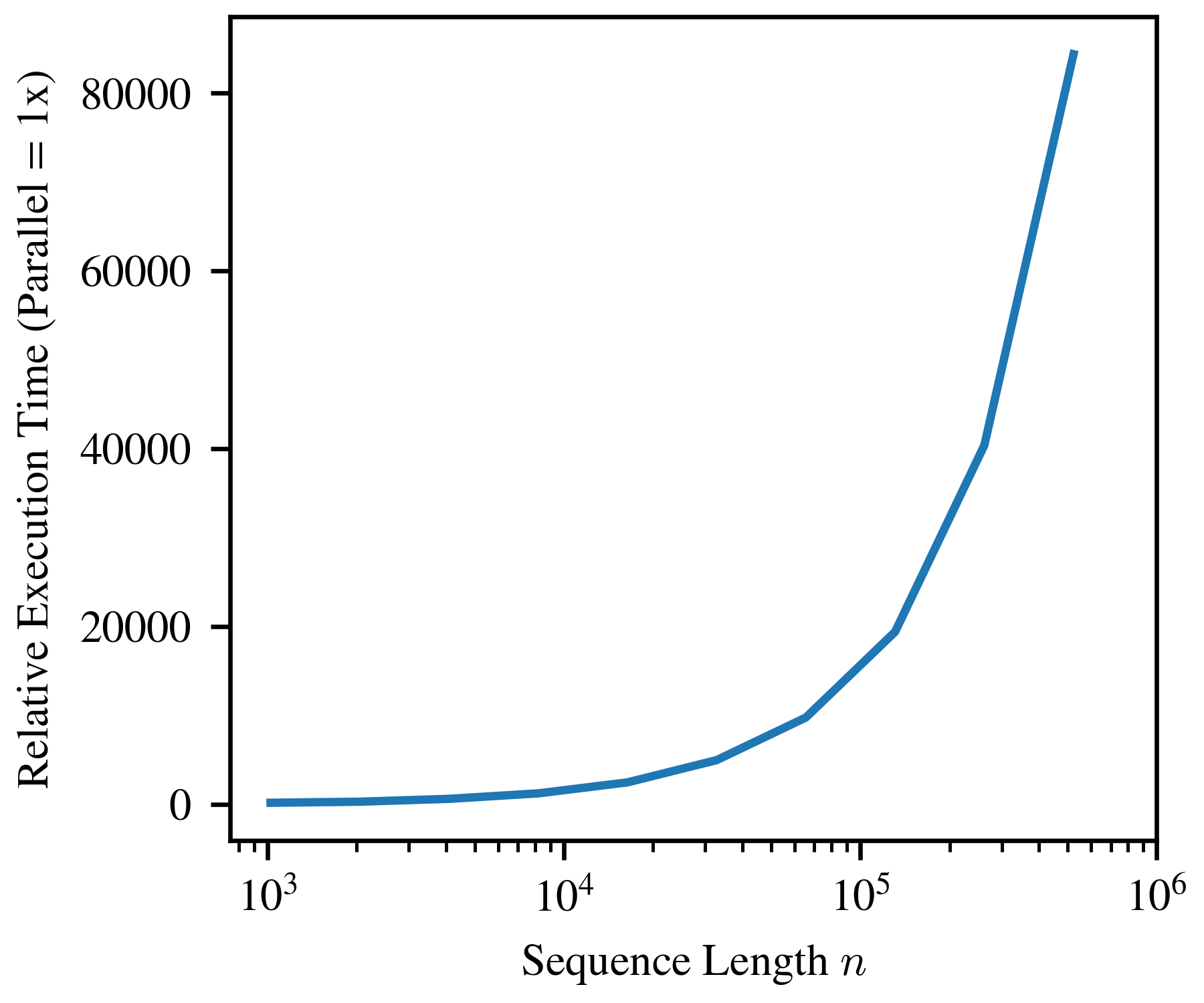
Figure 1: Time to compute $n$ elements sequentially, relative to parallel computation, on an Nvidia GPU. Each point is the mean of 30 runs.

We implement (3) in software. For numerical stability and slightly improved efficiency, we modify the computation of $x_{t}$ as follows:

$$x_{t}=e^{a^{*}_{t}+\operatorname{tail}(\operatorname{LCSE}(\operatorname{cat}(\log x_{0},\log b_{t}-a^{*}_{t})))},$$ (7)

where $\operatorname{cat}(\cdot)$ denotes concatenation, $\operatorname{tail}(\cdot)$ removes its argument’s first element, and

$$\operatorname{LCSE}(\cdot):=\log\overset{\text{{cum}}}{\sum}\exp(\cdot),$$ (8)

commonly provided as the “LogCumSumExp” function by software frameworks for numerical computing, applying the familiar log-sum-exp trick as necessary for numerical stability, and delegating parallel computation of the internal prefix sum to a highly-optimized implementation.

We test our implementation on parallel hardware and verify that it executes faster than sequential computation by a factor of $\frac{n}{\log n}$ (Figure 1).

References

• Blelloch (1990a) Guy E. Blelloch. 1990a. Prefix sums and their applications. Technical Report CMU-CS-90-190, School of Computer Science, Carnegie Mellon University.
• Blelloch (1990b) Guy E. Blelloch. 1990b. Vector Models for Data-Parallel Computing. MIT Press, Cambridge, MA.
• Hillis and Steele (1986) W. Daniel Hillis and Guy L. Steele. 1986. Data parallel algorithms. Commun. ACM 29(12):1170–1183.
• Ladner and Fischer (1980) Richard E. Ladner and Michael J. Fischer. 1980. Parallel prefix computation. J. ACM 27(4):831–838.