Evidence for the emergence of dust-free stellar populations at
Abstract
We present an analysis of the ultraviolet (UV) continuum slopes () for a sample of galaxy candidates at selected from a combination of JWST NIRCam imaging and COSMOS/UltraVISTA ground-based near-infrared imaging. Focusing primarily on a new sample of galaxies at selected from arcmin2 of public JWST imaging data across independent datasets, we investigate the evolution of in the galaxy population at . In the redshift range , we find evidence for a relationship between and absolute UV magnitude (), such that galaxies with brighter UV luminosities display redder UV slopes, with . A comparison with literature studies down to suggests that a relation has been in place from at least , with a slope that does not evolve strongly with redshift, but with an evolving normalisation such that galaxies at higher redshifts become bluer at fixed . We find a significant trend between and redshift, with the inverse-variance weighted mean value evolving from at to at . Based on a comparison with stellar population models including nebular continuum emission, we find that at the average UV continuum slope is consistent with the intrinsic blue limit of ‘dust-free’ stellar populations . These results suggest that the moderately dust-reddened galaxy population at was essentially dust free at . The extremely blue galaxies being uncovered at place important constraints on the dust content of galaxies in the early Universe, and imply that the already observed galaxy population is likely supplying an ionizing photon budget capable of maintaining ionized IGM fractions of per cent at .
keywords:
galaxies: evolution - galaxies: formation - galaxies: high-redshift - galaxies: starburst - dark ages, reionization, first stars1 Introduction
The capability of JWST to provide very-deep, near-/mid-infrared imaging and spectroscopy at is revolutionizing our understanding of the earliest galaxies. Prior to the launch of JWST, a small number of galaxy candidates had been discovered using the Hubble Space Telescope (HST) (e.g. Ellis et al., 2013; Oesch et al., 2016). Now, deep NIRCam imaging surveys are revealing hundreds of these systems (e.g. Harikane et al., 2023a; Finkelstein et al., 2022; Donnan et al., 2023a; Donnan et al., 2023b; McLeod et al., 2023; Robertson et al., 2023; Hainline et al., 2023). Moreover, growing numbers of these galaxies have already been confirmed spectroscopically (e.g. Arrabal Haro et al., 2023a, b; Bunker et al., 2023; Curtis-Lake et al., 2023; Harikane et al., 2023b). The discovery of a large abundance of galaxies at has been one of the key early results produced by JWST.
The fact that we are finding large numbers of galaxies, including a significant number of relatively ultraviolet (UV) bright objects (; e.g. Naidu et al., 2022; Castellano et al., 2023; Casey et al., 2023), represents a challenge for models of early galaxy formation. At the evolution of the UV luminosity function (LF) can be readily explained assuming no redshift evolution in the star-formation efficiency (e.g. Mason et al., 2015; Tacchella et al., 2018). If this model is extrapolated to , continued evolution of the UV LF is predicted, but this is in tension with the JWST observations (e.g. Harikane et al., 2023a). In fact, current constraints suggest that the UV LF does not evolve at all between and (at least at ; McLeod et al., 2023). A number of explanations for the non-evolving UV LF have been proposed including (i) an evolving star-formation efficiency, for example via a reduction in the stellar feedback efficiency at , including the potential for ‘feedback-free’ star formation (Dekel et al., 2023; Yung et al., 2023); (ii) a bias at these redshifts towards young, highly star-forming galaxies up-scattered with respect to the median UV magnitude versus halo mass relation (Mason et al., 2023; Shen et al., 2023); (iii) inherent uncertainties related to the spectral energy distributions (SEDs) of low-metallicity stellar populations (Inayoshi et al., 2022); and (iv) a transition to almost completely dust-free star-formation at (Ferrara et al., 2023; Ferrara, 2023; Ziparo et al., 2023). In this paper we present an analysis of the UV continuum SEDs of galaxies in the redshift range and investigate evidence for the last of these scenarios: dust-free star formation at .
It is well established that the stellar UV continuum, which can be described by a power-law ( for ), is an excellent probe of dust obscuration in star-forming galaxies (e.g. Calzetti et al., 1994; Meurer et al., 1999). In general, the UV continuum slope, , is sensitive to the light-weighted age, metallicity and dust attenuation of the population of massive stars in a galaxy (i.e. O- and B-type stars, with ages Myr). However, at the highest redshifts - and more broadly for all young star-forming galaxies - age and metallicity effects become subdominant, and is especially sensitive to dust (e.g. Tacchella et al., 2022). Indeed, this connection between and dust attenuation has been demonstrated directly in studies sensitive to infrared dust emission up to (see e.g. Bowler et al., 2023). By providing deep infrared imaging out to , JWST/NIRCam now enables robust estimates of for galaxies at (e.g. Cullen et al., 2023; Topping et al., 2023), probing dust in galaxies at the earliest cosmic epochs.
In an earlier work, we presented an initial examination of the UV continuum slopes of galaxies at selected from a combination of early JWST/NIRCam imaging and ground-based near-infrared imaging from COSMOS/UltraVISTA (Cullen et al., 2023). This initial sample comprised galaxies at a mean redshift of spanning a factor of in UV luminosity (). We found slopes that were, on average, bluer than their lower-redshift counterparts at fixed . These results had been tentatively anticipated with HST (e.g. Dunlop et al., 2013; Wilkins et al., 2016; Bhatawdekar & Conselice, 2021; Tacchella et al., 2022) and were in agreement with number of theoretical model predictions (e.g. Yung et al., 2019; Vijayan et al., 2021; Kannan et al., 2022). Independent JWST analyses painted a similar picture (e.g. Topping et al., 2022; Nanayakkara et al., 2023). These early studies of objects suggested stellar populations consistent with the young, low-metallicity and moderately dust-reddened stellar populations anticipated by theoretical models.
Here, we expand upon our initial analysis using a new sample of galaxy candidates at selected from a number of public JWST imaging surveys. Our new candidate set is built upon the sample presented in McLeod et al. (2023), which was used to robustly estimate the luminosity function. These new galaxy candidates are selected across arcmin2 of deep JWST/NIRCam imaging, which represents a increase in area compared to Cullen et al. (2023). As a result, we can now significantly improve upon our previous analysis in terms of the overall number of candidates. Crucially, our new sample now contains a significant number of galaxy candidates at , with an average redshift of , and enables us to place robust constraints on the evolution of up to .
The new analysis presented here complements the recent study of Topping et al. (2023), who present an investigation of the UV continuum slopes of galaxies up to in the JADES survey (Eisenstein et al., 2023), finding that by the average value of is extremely blue (). In this paper, we explore evidence for a similar trend in an independent sample of galaxies selected across a wide range of current JWST imaging datasets. Our sample is selected across an area larger than the full JADES area ( versus arcmin2) and, crucially, across independent, non-contiguous fields, thereby mitigating the effect of cosmic variance. While the JADES imaging used in Topping et al. (2023) is deeper, the increase in area means that our sample is on average brighter, and the resulting samples sizes at are comparable.
The paper is structured as follows. In Section 2 we describe the data and sample selection, and provide details of the sample properties and our method for determining . In Section 3 we present the results of our analysis, focusing on the evolution of with and absolute UV magnitude (). Our primary new finding is that by , the typical UV continuum slope of the galaxy population is extremely blue (). In Section 4 we discuss the implications of this result and demonstrate, based on an analysis of theoretical stellar population models, that the UV continuum slopes of galaxies at are consistent with dust-free star formation at this epoch. Finally, we summarise our main conclusions in Section 5. Throughout we use the AB magnitude system (Oke, 1974; Oke & Gunn, 1983), and assume a standard cosmological model with km s-1 Mpc-1, and .
2 Sample Selection and Properties
Our primary high-redshift galaxy sample is drawn from the wide-area JWST search for galaxies presented in McLeod et al. (2023). We additionally incorporated three further ultra-deep datasets not included in the original McLeod et al. (2023) sample: NGDEEP (Bagley et al., 2023), the first data release of the JWST Advanced Deep Extragalactic Survey (JADES, Eisenstein et al. 2023), and the additional arcmin2 region taken in parallel to the recent UNCOVER NIRSpec observations (hereafter “UNCOVER-South”). This primary sample was augmented by additional galaxies at drawn from COSMOS/UltraVISTA and JWST that were presented in our earlier work (Cullen et al., 2023). Below, we discuss the sample selection and properties of the various datasets used in this work.
2.1 The wide-area JWST sample
Our wide-area JWST sample was drawn from 15 independent publicly-available JWST imaging datasets within extragalactic fields, covering an on-sky area of . A list of these fields, including the proposal ID and PI name of each dataset is given in Appendix A (Table 5). We also include references to the relevant survey paper, ancillary data and lensing maps where applicable. With the exception of NGDEEP, JADES and UNCOVER-South, all of the datasets presented here are the same as those described in McLeod et al. (2023); we refer interested readers to Section 2 of McLeod et al. (2023) for a detailed description of the datasets in common.
Our inclusion of three new fields yields a further sources compared to the McLeod et al. (2023) sample. We have identified nine galaxy candidates at in our latest reduction of the NGDEEP observations (Bagley et al., 2023) (see below for candidate selection details). The NGDEEP dataset covers the HST UDF parallel 2 field, with another NIRCam module covering an adjacent area contained within the GOODS-South CANDELS footprint; we therefore supplemented the NGDEEP NIRCam imaging with the ACS F435W, F606W, F775W, F814W and F850LP imaging released as part of the Hubble Legacy Fields (Illingworth et al., 2013; Whitaker et al., 2019). We also included data from the first data release of the JWST Advanced Deep Extragalactic Survey (JADES, Eisenstein et al. 2023)111Accessed via https://archive.stsci.edu/hlsp/jades. The first data release (Rieke & the JADES Collaboration, 2023) covers the ‘deep’ portion of the imaging across an area of , from which we have selected a further galaxy candidates. Finally, we include candidates that were found in the arcmin2 of UNCOVER-South.
All of the JWST/NIRCam data in each field was reduced using the Primer Enhanced NIRCam Image Processing Library (pencil) software, a customised version of the JWST pipeline version 1.6.2 (Magee et al. in prep). The CRDS pmap varied slightly between each dataset owing to differences in the date on which the data were taken, reduced and analysed, although each pmap was sufficiently up-to-date () to take into account the most recent zero point calibrations. Again, we refer interested readers to McLeod et al. (2023) for a detailed description of the various pencil pipeline steps and full data reduction routine. In Appendix A (Table 6) we report the global 5 limiting magnitudes of the HST and JWST imaging in each field, calculated using 0.35diameter apertures and corrected to total assuming a point-source correction (see McLeod et al., 2023).

2.1.1 Construction of galaxy catalogues
Prior to galaxy candidate selection, we first homogenised the point-spread-function (PSF) of each of our images to match the PSF full width half maximum (FWHM) of the F444W imaging. This enabled us to measure consistent photometry across all of the photometric filters, removing any systematics arising as a result of differences in the PSF curve-of-growth.
For each of the datasets, we constructed multi-wavelength photometry catalogues by running Source Extractor (Bertin & Arnouts, 1996) in dual-image mode, performing aperture photometry in 0.35diameter apertures. Catalogues were created primarily with the F200W imaging as the detection band, although we also created additional F277W-, F356W- and F444W-detected catalogues in order to include any sources that had been missed due to a low signal-to-noise ratio (SNR) in the F200W imaging.
To calculate photometric uncertainties we adopted the method described in McLeod et al. (2023). We first generated a grid of non-overlapping apertures of diameter 0.35′′ spanning the full field-of-view and identified apertures corresponding to blank-sky using a Source Extractor segmentation map. For a given object, we measured the median absolute deviation (MAD) of the nearest blank-sky diameter apertures on an object-by-object basis, and scaled to the standard deviation using . We retained all sources detected at in our detection catalogues. Finally, to reduce potential contamination from artefacts, we required a detection in any one of the other detection bands.
We performed spectral energy distribution (SED) fitting on all sources in our initial catalogues using the SED fitting code LePhare (Arnouts & Ilbert, 2011), adopting the Bruzual & Charlot (2003) stellar population synthesis (SPS) library, a Chabrier (2003) IMF and the Calzetti et al. (2000) dust attenuation law. We modelled all sources assuming a declining star-formation history with ranging from to Gyr and stellar metallicities of and . We allowed to vary between and and accounted for IGM absorption using the prescription of Madau (1995).
We measured for each candidate from the best-fitting SED using a top hat filter centred on Å with Å. To correct our to total magnitudes, we scaled to the FLUX_AUTO measurements, and then applied an additional correction of per cent to account for light outside the Kron aperture (McLeod et al., 2023). For the cluster fields, we corrected for gravitational lensing by determining the magnification factor () using publicly available lensing maps (see Table 5). For fields where multiple lensing maps are available, we adopted the median value of across all maps. For UNCOVER-South, where no public lensing maps currently exist, we adopt a flat magnification, motivated by the typical values around the southern boundary of the Furtak et al. (2023) UNCOVER lensing map. While is unaffected by changes in , we include an additional systematic uncertainty in to account for this assumed floor.
2.1.2 High-redshift galaxy candidate selection
For our final sample, we first retained galaxies with a photometric redshift , a goodness of fit of , and at least between the goodness of fit of the primary redshift solution and secondary lower-redshift solution. In order to ensure a more robust final sample we then required a detection in at least one of the F150W, F200W or F277W filters. We also required a non-detection () in any of the F090W, F115W and HST ACS imaging filters that were available for a given dataset. In practice, the in F115W criterion restricts our sample to galaxies with . Where there was a lack of F115W imaging, we added a further criterion, whereby we required either a () non-detection in F150W, or at least a factor of two increase in flux between F150W and F200W. This last criterion confined us to redshifts for those datasets, but mitigated any potential contamination arising from F090W-F150W dropouts that have highly uncertain photometric redshifts. For each candidate, additional checks were performed using the photometric-redshift code EAZY (Brammer et al., 2008) as described in McLeod et al. (2023).
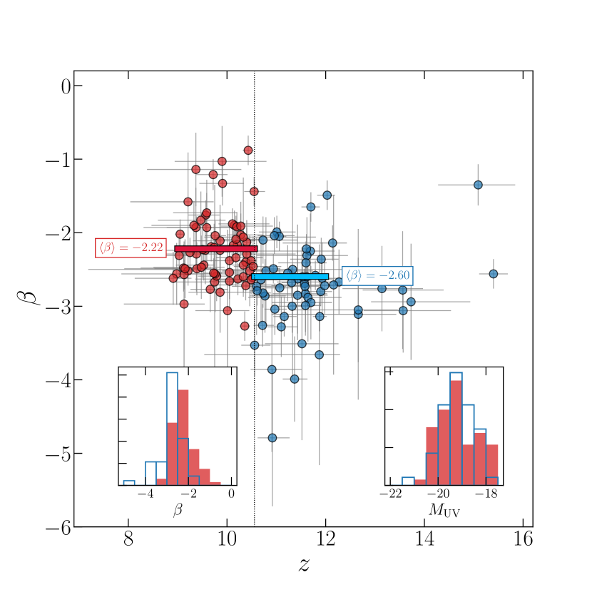
Across the fields we selected a total of galaxy candidates at . Throughout this paper we refer to these galaxies as our primary wide-area JWST sample. We use this sample to study the relationship between and redshift in Section 3.1. The distribution of and is shown by the blue data points in Fig. 1. The median values are and .
2.2 Additional galaxy candidates: the combined sample
The primary wide-area JWST sample was augmented using the sample analysed in our previous UV continuum slope study (Cullen et al., 2023). This sample was initially selected and presented in the UV luminosity function study of Donnan et al. (2023a) and combines a ground-based sample of bright galaxies at selected from the COSMOS/UltraVISTA field, and a JWST-selected sample at from early NIRCam imaging in SMACS J0723, GLASS and CEERS.
The selection criteria for this sample were less stringent (i.e. requiring only a detection in bands red-ward of the Lyman break; for full details see Donnan et al., 2023a) and therefore contained a number of candidates not selected in the new wide-area JWST sample. We retained the 35 galaxies from the Cullen et al. (2023) JWST sample that were not in our wide-area selection. We included all 16 galaxies from the ground-based COSMOS/UltraVISTA sample; these galaxies, although at a lower median redshift (), provide the valuable dynamic range in needed for studying the relationship between UV continuum slope and galaxy luminosity (see Section 3.2).
In total, we included galaxy candidates from the sample presented in Donnan et al. (2023a) and Cullen et al. (2023). The distribution of and for the COSMOS/UltraVISTA and JWST galaxies are shown by the red and yellow data points in Fig. 1 respectively. The median values for the COSMOS/UltraVISTA sample are and ; for the JWST sample the median values are and . We note that, due to the less stringent S/N constraints, these galaxies are less well-constrained in terms of and compared to our primary wide-area sample.
Combined with the primary wide-area sample, the total sample contains candidates at (Fig. 1); we refer to it as the ‘combined’ sample throughout this paper. This sample is primarily in our analysis of the relation in Section 3.2. The median values of absolute UV magnitude and redshift for the combined sample are and .
2.3 Measuring the UV continuum slope
The primary goal of this paper is to study the UV continuum slopes of our high-redshift galaxy candidates. The rest-frame UV continuum slope is characterised by a power-law index, , where . To determine , we modelled the galaxy photometry covering rest-frame wavelengths Å as a pure power-law including both the effects of intergalactic medium (IGM) absorption and the Ly damping wing. At Å, we modelled the effect of the Ly damping wing using the prescription of Miralda-Escudé (1998) (equation 2). At wavelengths below Ly (Å), we assumed complete IGM attenuation (i.e. ).
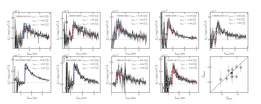
Our model consisted of three free parameters: (i) , the UV continuum slope; (ii) , the redshift of the galaxy and (iii) , the neutral hydrogen fraction of the surrounding IGM. To sample the full posterior distribution we used the nested sampling code dynesty (Speagle, 2020) assuming the following flat priors: ; and . Examples of fits to nine galaxies in our sample are shown in Fig. 2 (blue dashed lines).
We found that for a small minority of objects ( per cent of the full sample), our fits returned unrealistically small uncertainties () that significantly biased the population average estimates. Based on our -recovery simulations (Section 3.1.2), we found that for the typical global imaging depths of our dataset, could be recovered in the brightest sources () to within . We therefore adopted this value as a minimum floor on the uncertainty. Throughout this paper, unless otherwise stated, we also adopt the best-fitting redshifts and corresponding uncertainties derived from these fits in our analysis.
2.3.1 The effect of Ly damping wings and proximate DLAs
Evidence for Ly damping wings and even strong proximate damped Ly systems (DLAs) has been revealed from early JWST NIRSpec/PRISM spectroscopy of galaxies at (Curtis-Lake et al., 2023; Heintz et al., 2023; Umeda et al., 2023). Both effects act to soften the Ly break and are a potential source of systematic bias in our derived value of .
To account for the effect of the Ly damping wing, we included as a free parameter in our fits as described above. Although it is not possible to constrain from photometric data alone, our method enabled us to marginalise over the uncertainties on related to the unknown Ly damping wing strength. We found that marginalising over had a minor effect on our results relative to assuming a fixed value of ; the median value of became marginally redder () and the median uncertainties were unchanged. Object-to-object variations of up to were observed, but these were completely consistent with scatter due to the typical photometric uncertainties. Overall, we find that the average value of derived from broadband photometry is not strongly affected by the unknown strength of the Ly damping wing.
Recently, Heintz et al. (2023) presented evidence for excess DLA absorption in three galaxies at . These DLAs are likely due to large H i gas reservoirs in the interstellar and circumgalactic medium along the line-of-sight; crucially, they lead to an attenuation of flux redward of Ly in excess of the neutral IGM damping wing (see, for example, figure 1 of Heintz et al. 2023 and the discussion in Keating et al. 2023). We investigated the effect of DLA absorption by including a DLA at the source redshift with a neutral hydrogen column density of in our model and re-fitting the sample. This column density is the upper limit of the Heintz et al. (2023) measurements, and also at the upper end of the distribution measured from gamma ray burst (GRB) afterglow spectra (Tanvir et al., 2019). Again, we find that the overall effect on is negligible (median with respect to the default assumptions). The offset becomes more significant at the lowest redshifts where the difference between a DLA and the Ly damping wing is more pronounced. For sources at , the median offset is , however this is still not large enough to affect the results presented here.
2.4 Spectroscopic Sample
Nine galaxies in our primary sample had fully-reduced JWST NIRSpec/PRISM observations available through the DAWN JWST Archive (DJA)222https://dawn-cph.github.io/dja/index.html. We used these spectroscopic data to assess the accuracy of our photometric estimates.
The DJA reductions were performed using the grizli (Brammer, 2023) and msaexp (Brammer, 2022) software packages; basic details of the data reduction are presented in Valentino et al. (2023) and Heintz et al. (2023). The NIRSpec spectra were affected by wavelength-dependent slit-losses due to objects not being fully encompassed within the small MSA slitlets () and/or slit misalignment. To calibrate the 1D spectra we integrated them through the available NIRCam passbands and scaled the values to match the observed photometry, employing a linear interpolation between the each band. The nine flux-calibrated spectra are shown in Fig. 2.
The method for fitting from spectroscopic data is essentially the same as the method described above (Section 2.3). The only difference being that in this case the model is smoothed to match the resolution of the NIRSpec/PRISM data rather than integrated through the relevant photometric filters. To achieve the smoothing we first resampled the model to four pixels per full-width-half-maximum (FWHM) element and then convolved with a Gaussian with fixed pixel width of . Examples of these model fits are shown in Fig. 2.
2.4.1 Comparing and
In Fig. 2 we show the fits to the photometry (blue) and to the flux-calibrated spectroscopy (red) for the nine galaxies in our spectroscopic sample. In general we find excellent agreement between the two estimates. The lower right panel in Fig. 2 shows the versus comparison, where it can be seen that, for of the galaxies, the two values are consistent within . The inverse-variance weighted mean values of the two estimates are fully consistent, with and .
We find tentative evidence to suggest that, on average, is systematically smaller (bluer) than . For these cases in which , we find that the redshift estimated from the photometry is always larger than that estimated from the spectra, with . Our sample size is clearly small, but a tendency for to be systematically biased high at has been noted by other authors (e.g. Arrabal Haro et al., 2023a), which if confirmed might suggest a general bias towards bluer . However, our results suggests that the average effect is likely to be small (). Nevertheless, larger samples of deep NIRSpec/PRISM spectra will be helpful in order to accurately assess potential biases in due to systematics.
3 Results
| Sample | ||
|---|---|---|
| Wide-area (primary sample) | ||
| Combined (including Cullen et al., 2023) |
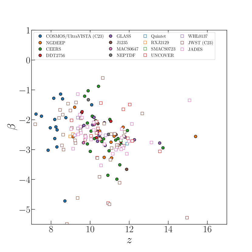
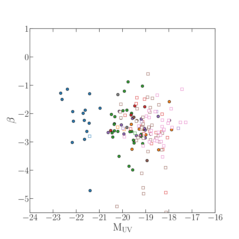
In Fig. 3 we plot the values for our combined sample as a function of redshift and and highlight the diverse selection of datasets used in this study. The range of values in our new wide-area JWST sample is consistent with that presented in Cullen et al. (2023), with measured values between and , and we observe a number of similar features in the data.
Firstly, we again see a large scatter in , with individual estimates as blue as . These extremely blue values () are driven, at least in part, by the well-known blue bias in estimates at faint magnitudes (e.g. Dunlop et al., 2012; Rogers et al., 2014; Cullen et al., 2023) and by the significant uncertainties on individual objects (the median uncertainty for the combined sample is ). Unsurprisingly, the scatter is noticeably reduced in our higher S/N wide-area sample, which contains fewer extremely blue outliers; for example, per cent of the Cullen et al. (2023) sample have compared to per cent of the wide-area sample. Nevertheless, it is important to note that the existence of objects with even in robust, high S/N, samples emphasises the necessity of adopting empirical approaches to measuring that will not artificially truncate the full observed distribution (as can happen when measuring via fitting stellar population models; see e.g. Rogers et al., 2013).
In Table 1 we report the inverse-variance weighted mean values for the primary sample and for the combined sample. For our primary sample we find . As in Cullen et al. (2023), we prefer the weighted mean over a simple median in order to mitigate against the blue bias in the scatter at faint magnitudes (this blue scatter is clearly visible in the bottom panel of Fig. 2). For the combined sample (i.e. including the Cullen et al., 2023 sources) we find . This marginally redder value is primarily due to the inclusion of bright objects at from the ground-based COSMOS/UltraVISTA survey in the combined sample, as well as the slightly lower median redshift (see Fig 1, and the results presented in Sections 3.1 and 3.2 below).
The values reported in Table 1 are somewhat bluer than the value of we reported in Cullen et al. (2023). This is in part due to the fact that the new sample is marginally fainter, but the main reason is the greater proportion of candidates at . In our new wide-area JWST sample: per cent () of candidates have , compared to 43 per cent () in Cullen et al. (2023). It is this difference in the fraction of candidates that drives the difference in . The implication here is that galaxies at are significantly bluer and indeed this can be seen in Fig. 3. We investigate the trend between and redshift in detail below.
It is worth noting that as in Cullen et al. (2023) the full sample average values reported in Table 1 are not more extreme than the bluest galaxies observed in the local Universe (e.g. NGC 1705; , ; Calzetti et al., 1994; Vázquez et al., 2004). As will be discussed below, we still find that up to the typical value of is consistent with the bluest values found locally. However, a new crucial finding of this paper is that at we now find strong evidence to suggest that a significant fraction of galaxies have extremely blue UV continuum slopes ; this represents the extreme blue end of objects observed in the local Universe, but our results suggest this is the typical value of for galaxies at with absolute UV magnitudes in the range .
In the following, we present a detailed analysis of the UV continuum slopes of our galaxy candidates and their dependence on redshift and UV luminosity (). We begin in Section 3.1 by investigating the evolution of with redshift and present the main result of this work. Then, in Section 3.2, we derive the relation as a function of redshift for our sample, providing an update on the relation derived in Cullen et al. (2023).
3.1 The evolution of with redshift
An evolution to bluer UV colours at higher redshifts is expected as galaxies become progressively metal and dust-poor at earlier cosmic times. Prior to JWST, this trend had been observed up to (e.g. Finkelstein et al., 2012; Bouwens et al., 2012, 2014). Recently, Topping et al. (2023) have presented evidence for continued evolution beyond , finding extremely blue average UV slopes of at (we discuss the comparison between our results and Topping et al., 2023 below).
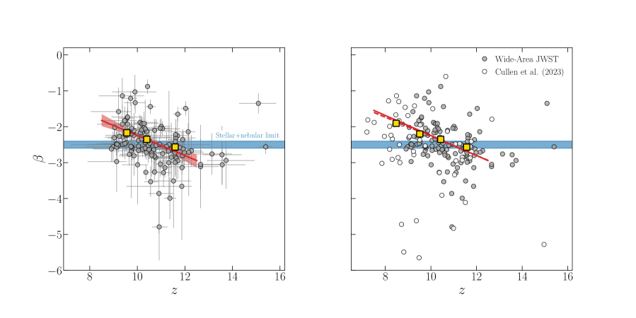
In Fig. 4 we show the relation for our primary sample (left-hand panel) and combined sample (right-hand panel). Focusing first on the primary sample, it can be seen that we observe a clear trend in our data, with becoming progressively bluer at higher redshifts. Fitting a linear relation to the individual data points (and accounting for the uncertainties in both and ) yields
| (1) |
where we have restricted the fit to due to the lack of candidates at higher redshifts. We also show in Fig. 4 the inverse-variance weighted mean values in bins of redshift; these binned values (reported in Table 2) are fully consistent with the fit to the individual objects. We see that the typical changes from at to at , a relatively rapid evolution of across just Myr of cosmic time.
| Redshift range | |||
|---|---|---|---|
| Wide area sample | |||
| Combined sample | |||
The redshift evolution observed in Fig. 4 is unlikely to be strongly affected by differences in the typical as a function of redshift. Significant differences in could result in a bias due to the known relation between and that has been demonstrated in numerous studies across all redshifts (e.g. Rogers et al., 2014; Bouwens et al., 2014; Cullen et al., 2023; the relation for our new sample will be derived in Section 3.2). However, Fig. 1 already clearly shows that the distribution of the primary sample is not strongly evolving between and . From Table 2, it can be seen that the difference in between adjacent redshift bins is roughly . Assuming (see Cullen et al., 2023 and Section 3.2 below), this translates to , which is smaller than the observed differences in Table 2. In Section 3.1.2 below, we provide further detailed discussion of possible selection effects and measurement biases present in our analysis and conclude that the steep trend is indeed a real feature of our data.
Including the additional candidates from the combined sample, we find they they are fully consistent with the relation derived from the primary wide-area JWST sample (right-hand panel of Fig. 4). At , the JWST-selected galaxies from Cullen et al. (2023) follow the same trend; in particular, it can be seen that the these candidates also show extremely blue UV slopes at . At , the addition of the ground-based COSMOS/UltraVISTA candidates from the Cullen et al. (2023) sample provides an extra redshift bin at . The value of in this bin is consistent with an extrapolation of Equation 1. However, we note that the galaxies in the redshift bin are significantly brighter by , meaning the average is likely biased with respect to the higher redshift bins (by up to ). Accounting for this bias would suggest that the evolution between to is likely to be shallower if compared to a sample matched in magnitude. The focus of this paper is the evolution in at , but future JWST studies will enable a robust determination of the redshift evolution of in magnitude-matched samples to lower redshfits.
3.1.1 The transition to extremely dust-poor stellar populations
The key result of this paper, highlighted in Fig. 4, is that by the average UV continuum slope of the galaxy population at 333Assuming the fixed faint-end slope UV LF fit of McLeod et al. (2023) this range corresponds to . The average absolute UV magnitude of our sample at () corresponds to . is consistent with the ‘dust-free’ limit expected from standard stellar population models and nebular physics. As we discuss in more detail in Section 4.1, this limit assumes a young, dust-free, stellar population surrounded by ionized gas such that the ionizing continuum escape fraction is 0 per cent and the strength of the nebular continuum emission is maximised. Under these assumptions, the bluest UV continuum slopes expected are to (e.g. Robertson et al., 2010; Cullen et al., 2017; Reddy et al., 2018), a theoretical limit that appears to be validated by observations of dust-poor local star-forming galaxies (e.g. Chisholm et al., 2022). Any value bluer than this limit implies a non-zero escape fraction of ionizing photons. Crucially, since dust acts to redden 444 where for standard dust attenuation curve assumptions (e.g. Calzetti to SMC; McLure et al., 2018)., this limit also implies that it is extremely difficult to obtain UV slopes of in the presence of dust. As can been seen in Fig. 4, our results suggest that this limit is being reached by , implying that galaxies at this redshift are uniformly extremely dust-poor, and potentially dust-free.
The rapid transition to extremely blue values at the highest redshifts in our sample is highlighted further in Fig. 5. Considering the steep nature of the relation (Fig. 4), we fitted a toy model to our wide-area JWST sample with the following form:
| (2) |
where is the redshift at which the population-average value of transitions from to . Although this model is not physically motivated, it does at least give a useful indication of the approximate redshift above which galaxies are becoming uniformly extremely blue.
Fitting the model in Equation 2 to our primary wide-area sample yields:
| (3) |
The fit is shown in Fig. 5. Again, we can be confident that this difference in is not strongly biased due to differences in by comparing the distribution above and below . The inset panel of Fig. 5 (lower-right) shows that the distributions of upper and lower redshift samples are fully consistent; both have and a standard KS test returns a significance (value) of , consistent with the null hypothesis that both samples are drawn from the same distribution.
Interestingly, we find that the step function model (Fig. 5) provides a better fit to our data than the linear model (Fig. 4). However, based on the reduced chi-squared values (), neither model provides a formally statistically-acceptable fit. For the linear model we find compared to for the step function model. These large values are most likely due to a large intrinsic scatter in at fixed redshift. A given redshift bin will span a range of UV magnitude with a width of (Fig. 1), corresponding to assuming (Section 3.2; Cullen et al., 2023). Considering this, the fact neither fit is formally acceptable is not especially concerning. Although neither fit can be preferred, it is nevertheless intriguing that the current data prefers a sharp transition above . Larger samples, ideally with a larger fraction of robust spectroscopic redshifts, will be able to clarify the precise nature of the rate of evolution at .
Taken together, the model fits in Figs. 4 and 5 suggest that at the typical UV continuum slope of galaxies is . This implies that the galaxy population, across a relatively wide range of , is consistent with the ‘dust-free’ limit suggested both by theoretical models and observations of local galaxies. Moreover, our data also suggest that the transition to these extremely blue slopes occurs over a narrow redshift range, with galaxies at having on average blue, but not particularly extreme, UV continuum slopes of , consistent with a moderate amount of dust attenuation (, assuming ; see McLure et al., 2018). Taken at face value, this implies a rapid build up of dust in galaxies within the Myr time frame between and . Finally, as we discuss further in Section 4.1, these observations appear to be consistent with models that predict an efficient ejection of dust in the earliest phases of galaxy formation (Ferrara et al., 2023; Ziparo et al., 2023), negligible amounts of dust being formed in the first phases of star-formation (Jaacks et al., 2018) or efficient dust destruction at the highest redshifts (e.g. Esmerian & Gnedin, 2023).
| range | |||
|---|---|---|---|
3.1.2 Selection effects and measurement bias
It is worth considering the possibility that the extremely blue UV slopes at are a result of selection effects and/or measurement biases. Indeed, the measurement of from broadband photometry is known to be affected by subtle biases. For example, the bias towards bluer values of at faint UV magnitudes has been extensively documented (e.g. Bouwens et al., 2010; Dunlop et al., 2012; Rogers et al., 2014). In Cullen et al. (2023), we found that for our JWST sample the average value of was biased toward bluer values at . If we apply the relation derived in Cullen et al. (2023) to the median of the high- and low-redshift redshift splits in Fig. 5 (i.e. ) we find that these estimates could be biased blue by 555In general, the bias in as a function of depends on the details of the selection method. However, although the selection method of our new wide-area JWST sample is different to the selection method applied in in Cullen et al. (2023) we have confirmed that the bias is similar.. A bias at this level would clearly not affect our results. We have also confirmed that the same steep redshift- trend remains if we restrict our sample to the brightest galaxies in our wide-area JWST sample with (i.e. those which should not be affected by a measurement bias). We therefore conclude that is unlikely that our results are driven by a blue bias due to faint galaxies.
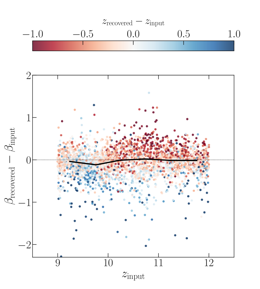
We have also explored potential redshift-dependent biases which might arise from the fact that different combinations of filters are used - and different portions of the UV spectrum are sampled - depending on the redshift of the candidate. For example, the UV continuum is sampled by the F150W, F200W and F277W filters at , compared to the F200W, F277W and F356W filters at . To test for a redshift bias we ran a simple simulation in which we first constructed simple power-law SEDs with an intrinsic slope of spread uniformly across the redshift range and the range . We then applied IGM attenuation using the prescription of Inoue et al. (2014). Photometry was generated in each of the observed filters (see Appendix Table 6) and scattered according the the typical imaging depths (averaging the depths across multiple fields where appropriate). The ‘observed’ UV continuum slopes () were then recovered for the simulated galaxies that met our selection criteria.
The resulting bias as a function of redshift is shown in Fig. 6. It can be seen that we do not observe a strong redshift-dependent effect. The largest bias () is seen in a narrow redshift interval around , which corresponds to the redshift at which the Lyman break passes between the F115W and F150W filters. At this specific redshift, the photometric redshift is almost uniformly biased high, resulting in an underestimate of the true UV slope. In general, the bias across all redshifts is negligible () and crucially at there is no evidence or a strong blue bias.
It is also clear from Fig. 6 that the scatter is driven primarily by photometric redshift uncertainty. When the photometric redshift is underestimated, is overestimated, and vice versa. We find that typical scatter in the recovered at all and is , which motivates our decision to set this a minimum error floor on individual estimates (see Section 2). Clearly, obtaining robust spectroscopic redshifts will be key in driving down uncertainties and confirming the results presented here.
Finally, we find that our results are also unlikely to be driven by selection effects. This is partly highlighted by the similarity of the distributions above and below in Fig. 5, which demonstrates that our sample selection does not favour intrinsically fainter, and hence bluer, objects in the higher redshift bins. As an additional check, we ran a slightly altered version of the simulation above in which galaxies were generated with a uniform distribution in between and . This simulation confirmed that our selection criteria recovered the underlying uniform distribution in at all redshifts (e.g. we do not see a bias to bluer at introduced by our selection).
In summary, we conclude that our primary result that by the galaxy population is uniformly extremely blue, with - is not strongly affected by selection effects and/or measurement biases. Moreover, multiple independent studies are now coming to similar conclusions (Austin et al., 2023; Topping et al., 2023; Morales et al., 2023). Although our data suggest a rapid evolution in between and , larger samples are needed to robustly quantify the exact trend across this short ( Myr) span of cosmic time.
3.2 The relation at
The relation, or colour-magnitude relation, traces the variation of the dust and stellar population properties of galaxies as a function of their UV luminosity. Observations up to have shown that a correlation exists, such that fainter galaxies are on average bluer (e.g. Finkelstein et al., 2012; Rogers et al., 2014; Bouwens et al., 2014; Cullen et al., 2023; Topping et al., 2023). These observations suggest that fainter galaxies are typically younger and less dust- and metal-enriched, in agreement with predictions of theoretical models (e.g. Vijayan et al., 2021; Kannan et al., 2022).
In Cullen et al. (2023) we provided a fit to the a sample of galaxies at . Due to the small sample size in Cullen et al. (2023), in this initial fit we included all galaxies across the full redshift range of the sample from to 666The candidate has subsequently been shown to be a interloper (Arrabal Haro et al., 2023b), although the inclusion of this object does not affect the fit in Cullen et al. (2023).. We found evidence for a relation with . This slope is consistent with the slope measured for large samples at lower redshift, for example the relations of Bouwens et al. (2014) and Rogers et al. (2014) which have and respectively. However, we found that the normalisation for the relation was lower at , such that galaxies are on average bluer by compared to .
| Redshift range | ||
|---|---|---|
| (fixed) | ||
| (fixed) |
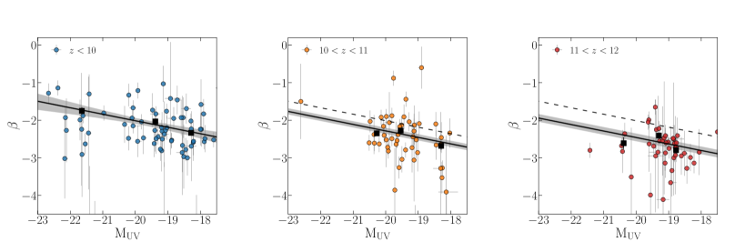
With our enlarged sample we are now in a position to investigate the redshift evolution of the relation at . For the analysis in this section we make use of the combined sample which includes the COSMOS/UltraVISTA galaxies at . These ground-based candidates trace the bright end of the UV luminosity distribution () and are therefore crucial in providing a large dynamic range in (see Fig. 1). To investigate the redshift evolution of the relation, we split our sample into three bins of redshift; for each redshift bin, we then calculated the inverse-variance weighted mean in three bins of . The resulting , and values are given in Table 3.
In practice, only the redshift bin has sufficient dynamic range in (from to ; Fig. 7) to enable an accurate estimate of the slope of the relation. In this redshift range, there is clear evidence for a dependence, with evolving from at the brightest magnitudes (median ) to at the faintest magnitudes (median ). The best fitting colour-magnitude relation to the individual candidates (blue data points in Fig. 7) is
| (4) |
where we have accounted for the uncertainties in both and . In this formulation the intercept, , represents the typical value of at . Our new best-fitting relation is consistent with the fit in Cullen et al. (2023), which is perhaps unsurprising since (i) at the bright end both samples are identical (i.e. the COSMOS/UltraVISTA candidates) and (ii) the majority of candidates in Cullen et al. (2023) fall within the same redshift interval. However, we now find evidence for a non-zero slope at a significance of , compared to previously. We note that the median redshift of the galaxies at the bright end () is lower than the median redshift in the fainter bins (by ), which may introduce a bias if there is a significant redshift evolution in over that redshift interval. However, we see no evidence for this in Figs. 4 and 5. Nevertheless, the clear lack of galaxies at and with JWST photometry is something that will hopefully be addressed with current and future wide-area surveys (e.g. Casey et al., 2023; Franco et al., 2023).
In the two higher redshift bins we cannot constrain the slope at the level due to the lack of galaxies with (see Fig 7). Fitting the data in the bin yields . Reassuringly, this slope is fully consistent with the slope derived at , although the uncertainty is clearly much larger. Looking at the inverse-variance weighted mean values in Table 3, we find an evolution from in the faintest bin to in the brightest bin. Again, based on the uncertainties, the significance of this difference is at the level. In the highest redshift bin (), the data do not show any evidence for a relation. A formal fit yields and the difference between the brightest and faintest bins is also only significant at the level. Nevertheless, given the significant uncertainties, the data remain consistent with within .
In light of the relative lack of constraints at , we assumed a fixed slope of at these redshifts and fitted only for . This approach yields at and at (where the uncertainties account uncertainty in the slope). The two fits are shown in Fig. 7. These results again highlight the main finding of this paper: at fixed , the typical value of is evolving rapidly with redshift between and , reaching at the highest redshifts. The resulting best-fitting parameters are given in Table 4.
In summary, we find convincing evidence () for a relation in our sample at with a slope of . This slope is slightly steeper than, but consistent with, the slope derived at (e.g. Bouwens et al., 2014; Rogers et al., 2014). Our results currently suggest that the slope of the relation is already set within the first Myr of cosmic time, and does not evolve strongly thereafter. At we lack the dynamic range in to constrain the slope, however assuming a fixed , we find that the normalisation evolves rapidly from at to at .
3.2.1 Comparison to the literature
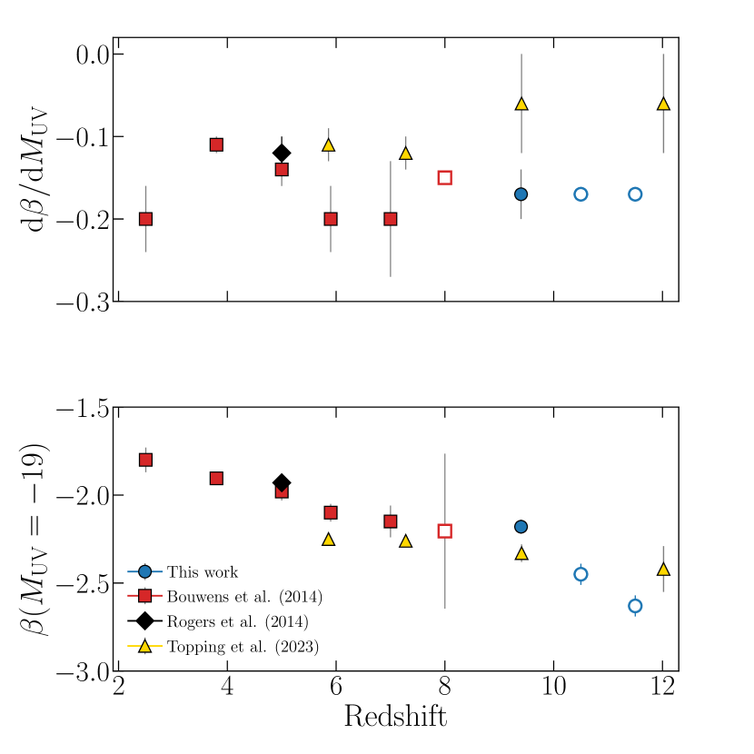
In Fig. 8 we show a compilation of derived slopes and intercepts for the relation in star-forming galaxies from to . The compilation includes the results of this work and three literature studies: Bouwens et al. (2014), Rogers et al. (2014) and Topping et al. (2023)777This selection of literature sources shown in Fig. 8 has been restricted for clarity and is therefore not comprehensive. However, the general picture remains unchanged if other studies are included (e.g. Finkelstein et al., 2012; Dunlop et al., 2013; Bhatawdekar & Conselice, 2021). At , the majority of the constraints come from the large HST study of Bouwens et al. (2014)888We note that the constraint reported in Bouwens et al. (2014) and shown in Fig. 8 was first derived in Bouwens et al. (2009).. Applying a consistent analysis across the full redshift range, Bouwens et al. (2014) find a gradual decline in the normalisation of the relation from at to at ; an evolution of across Gyr of cosmic time. Their derived slopes are scattered in the range , which is consistent with the general pattern followed by all datasets in Fig. 8. The inverse-variance weighted mean value of the slope across all redshifts in Bouwens et al. (2014) is . We also show the wide-area () analysis at of Rogers et al. (2014) which, given the total sample size and area, is the benchmark constraint on at this redshift. Rogers et al. (2014) find and , in excellent agreement with the constraints of Bouwens et al. (2014). We therefore consider the constraints a robust anchor with which to compare the data at higher redshifts.
We also show the recent determinations of the relation across the redshift range from Topping et al. (2023). Their analysis is based on deep JWST/NIRCam observations (taken as part of the JADES survey) and is therefore directly comparable with ours. In their two bins at ( and ), Topping et al. (2023) report an essentially flat slope with (at the slope is fixed to the value). At , this contrasts with our determination of . The difference may be attributable in part to the lack of bright-end constraints in Topping et al. (2023): their brightest bin has an absolute UV magnitude of , whereas our sample probes to thanks to the inclusion of the COSMOS/UltraVISTA sample (Fig. 1). However, if we restrict our sample to , we still see evidence for a slope of (Fig. 7). Formally, however, the tension is not significant, and the two constraints are consistent within . At our results are in relatively good agreement agreement given the uncertainties. Crucially, Topping et al. (2023) also find that by the galaxy population is uniformly extremely blue.
Although tensions between the various studies exists, these differences are not highly significant (i.e. none of current constraints at fixed redshift are incompatible at the level). The general picture discernible from Fig. 8 is of a relatively shallow relation that is in place from at least out to , with a fixed (or at least slowly evolving) slope, probably in the range . At more data are still needed to robustly constrain this slope, although current data are compatible with a slowly-/non-evolving scenario. In contrast, the normalisation of the relation is clearly changing, with galaxies at fixed becoming bluer towards higher redshift. Based on our results, the evolution is gradual to out , with evolving from at to at . At , the evolution becomes more rapid (especially when framed in terms of cosmic time), reaching by . The analysis of Topping et al. (2023) suggests a more gradual evolution, but still suggests that by the galaxy population is uniformly extremely blue. The rate of decline of therefore remains an open question, but there is a consensus that, by , the typical UV slope at approaching the ‘dust-free’ limit of to .
4 Discussion
We have presented an investigation of the UV continuum slopes of a sample of galaxy candidates at , with the aim of understanding the dependence of on redshift and . The primary focus of our analysis has been a new wide-area sample of galaxies at selected from public JWST/NIRCam imaging datasets (covering an on-sky area of arcmin2). The main result of this work is that we find a strong redshift evolution of in our wide-area sample, with a rapid transition from at to at (Figs. 4 and 5). The population-average value of at is consistent with expectations for extremely dust poor, even dust-free, stellar populations (see discussion below). We then investigated the relation using our full sample of galaxies which included the bright () ground-based candidates at from COSMOS/UltraVISTA. We find strong evidence () for a relation at with a slope of , similar to the slope observed at lower redshifts (Figs. 7 and 8). At , our data are not sufficient to accurately constrain the slope due to a lack of bright galaxies; however our analysis confirms a rapid evolution in the normalisation of the relation across the redshift range . In this section, we discuss the ‘dust-free’ galaxy interpretation and consider the implications for dust formation in the early Universe and cosmic reionization.
4.1 A transition to dust-free star-formation at ?
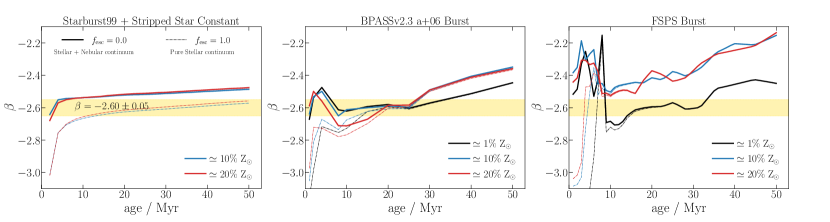
The bluest/steepest possible value of is set by the intrinsic stellar spectrum of young metal-poor galaxies. At the youngest ages ( Myr) and lowest metallicities ( per cent solar) the UV slope can reach values as blue at (e.g. Bouwens et al., 2010; Robertson et al., 2010; Stanway et al., 2016; Topping et al., 2022). However, the presence of ionized gas in galaxies will result in continuum emission as a consequence of free-free, free-bound and two-photon processes (i.e. the nebular continuum). This nebular continuum acts to redden the UV continuum slope (e.g. Byler et al., 2017). Models suggest that the bluest expected UV slopes when accounting for the nebular continuum emission are (e.g. Stanway et al., 2016; Topping et al., 2022).
We reproduce this result for a selection of stellar population synthesis models in Fig. 9 where we plot as a function of stellar population age. The stellar populations considered are starburst99 continuous star-formation models including a contribution from stripped stars (Leitherer et al., 1999; Götberg et al., 2018), bpassv2.3 single-burst models including -enhanced abundance ratios (Byrne et al., 2022) and Flexible Stellar Population Synthesis (fsps) single-burst models (Conroy et al., 2009; Conroy & Gunn, 2010; Byler et al., 2017). Full details of the nebular continuum modelling are given in Appendix B. It can be seen that although variations exists between each model, the overall picture is consistent: when an escape fraction () of 0 per cent is assumed (i.e. all of the ionizing photons emitted by the stellar population are converted into nebular emission) the bluest expected UV continuum slope is . Moreover, this only occurs for the youngest ages Myr. If a non-zero is assumed, then bluer slopes are possible, with a minimum value of , but this occurs at ages of and for an escape fractions close to 100 per cent (i.e. pure stellar emission).
Another notable feature of Fig. 9 is that the youngest, most metal-poor, stellar populations produce the strongest nebular continuum emission. This occurs because these stellar populations produce harder ionizing spectra. In some cases the strong nebular emission can entirely compensate for their intrinsically bluer stellar UV slopes. For example, considering the FSPS models (right-hand panel of Fig. 9), the UV continuum slopes including nebular continuum emission are actually redder at the youngest ages. From this we can conclude that invoking more extreme stellar populations with harder ionizing spectra (i.e. top-heavy IMFs, Pop-III stars) is unlikely to result in UV slopes intrinsically bluer than when the effects of nebular continuum emission are included.
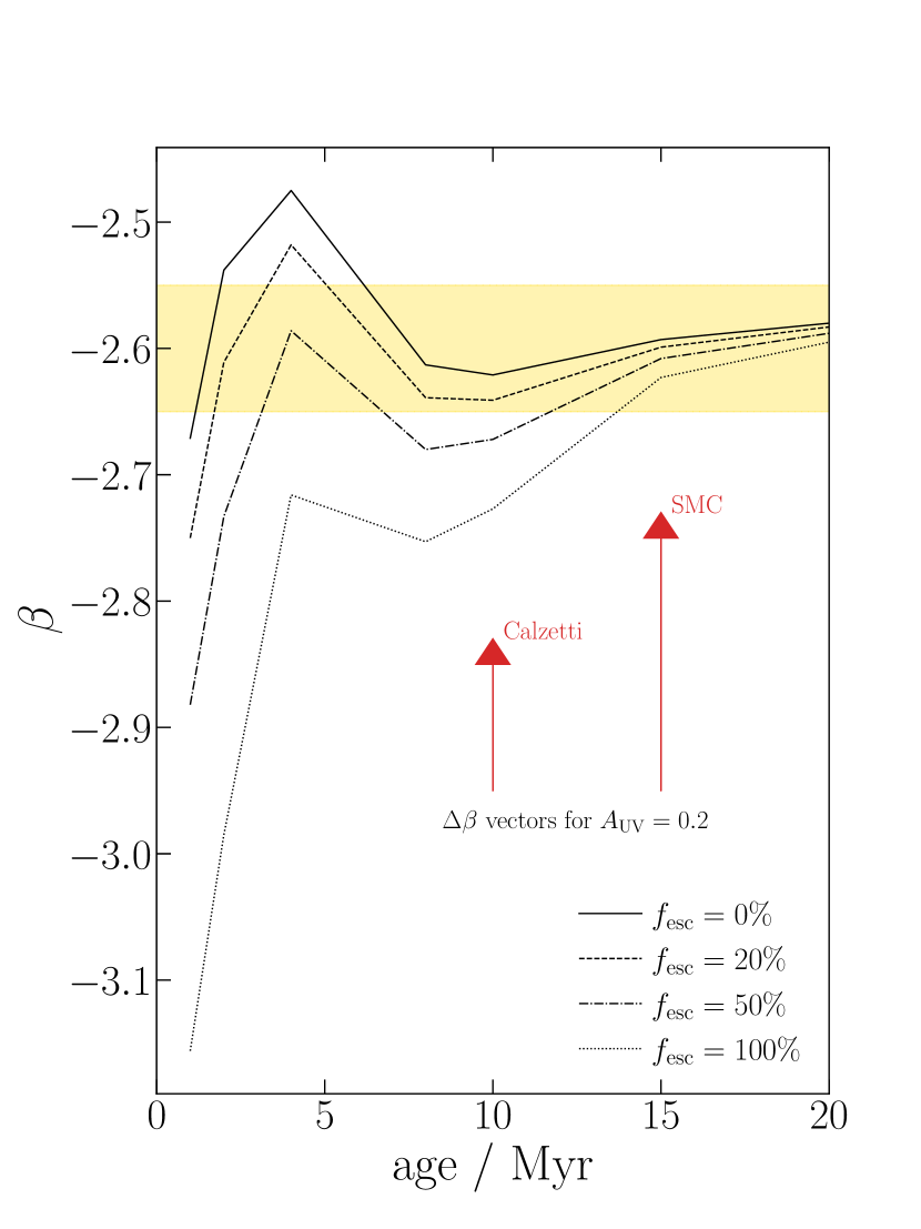
The model predictions in Fig. 9 imply that a stellar population with an observed UV continuum slope of is almost certainly experiencing negligible (essentially zero) dust attenuation, regardless of age. For a stellar population to be dust-attenuated yet still have would require a counter-intuitive scenario in which a significant fraction of ionizing continuum photons are escaping into the IGM in the presence of dust. We highlight this argument in Fig 10, where we show versus stellar population age for a bpassv2.3 burst model across a range of values. Even for extreme escape fractions of per cent, the intrinsic UV continuum slope only falls below at the very youngest ages (i.e. Myr). To achieve including dust would therefore require a very young, dominant, burst with a large ( per cent) escape fraction which is at the same time experiencing magnitudes of UV attenuation. Although we cannot completely rule such a scenario out (i.e. for very specific star/gas/dust geometries) the degree of fine-tuning required renders it unlikely.
Indeed, it is arguably more likely that the stellar population ages are Myr such that these galaxies have intrinsic UV continuum slopes including nebular continuum emission of (Fig. 9). In Cullen et al. (2017) we analysed the stellar populations of simulated galaxies at and found that the typical intrinsic UV slopes assuming were for galaxies with light-weighted stellar ages between Myr and Myr. Light-weighted ages of up to Myr are clearly plausible at as this would correspond to a formation redshift of and galaxies at this redshift have already been spectroscopically confirmed by JWST (Curtis-Lake et al., 2023). Therefore, it is possible, and even likely, that the typical intrinsic slopes of the galaxies in our sample are redder than (for ). In this case, an observed UV continuum slope of indicates both negligible dust attenuation and a non-zero escape fraction of ionization photons. We discuss implications for the escape fraction and reionization in more detail below.
Finally, it is worth acknowledging that our constraints are formally consistent a value as red as within the uncertainties (). Assuming an intrinsic slope of (i.e. an extremely young burst) this value would correspond to an upper limit of depending on the assumed attenuation curve (McLure et al., 2018). However, for older and/or composite stellar populations (with ), the implied upper limit on the UV attenuation would be closer to . Nevertheless, our formal best estimates are most consistent with negligible, essentially zero, dust attenuation. Below we consider some physical interpretations of dust-free systems in the young Universe.
4.1.1 The physical motivation for ‘dust-free’ galaxies
The above comparison with theoretical UV spectra models suggest the average value we observe at are consistent with the expectation for dust-free stellar-populations. It is important to ask whether such a scenario physically plausible. Dust is formed in the ejecta of core-collapse supernovae (e.g. Todini & Ferrara, 2001), and as a result galaxies might be expected to accumulate dust immediately after the onset of star-formation. In this case, a mechanism for either ejecting or destroying dust formed in supernovae is required to explain the absence of dust in star-forming galaxies. Ferrara et al. (2023) and Ziparo et al. (2023) propose one potential scenario in which intense UV radiation pressure from ongoing star-formation in these early galaxies drives dust out of the interstellar medium (see also Nath et al., 2023). Most recently, Ferrara (2023) have postulated that above the specific star-formation rate of galaxies crosses a threshold above which powerful radiation-driven outflows are capable of clearing dust from the ISM. Intriguingly, this is the same redshift threshold above which we begin to see uniformly extremely blue colours of in our sample.
An alternative hypothesis, proposed by Jaacks et al. (2018), is that the first generation of star-formation (Pop-III stars) produce negligible amounts of dust. In this scenario the stars at are either forming from recently enriched but dust-free Pop-III gas, or alternatively we are seeing the effect of a significant fraction of current Pop-III star-formation in our sample. Indeed, Jaacks et al. (2018) estimate for Pop-III SEDs. We note however that, other than their blue UV continuum slopes, the NIRSpec/PRISM spectra shown in Fig. 2 do not show any obvious Pop-III signatures in their FUV spectra (e.g. strong broad He ii emission). Finally, it is also possible that dust is more efficiently destroyed in the earliest star-forming systems. Current estimates of dust grain destruction rates in the ISM vary by up to an order of magnitude due to different assumptions regarding dust mircrophysics (e.g. grain-grain collisions and shattering; Kirchschlager et al., 2022, e.g.). It is possible that specific physical conditions at could result in enhanced dust destruction (e.g. enhanced SFR surface densities) although direct evidence is currently lacking. The dust destruction scenario is supported by the theoretical analysis of Esmerian & Gnedin (2023), who used a cosmological fluid-dynamical simulation of galaxies within the first 1.2 Gyr () to investigate the effect of different dust models. A comparison of our UV slope measurements up to with their model favours enhanced dust destruction with destruction rates elevated by an order of magnitude or more relative to default assumptions. There are therefore a number of possible physical processes which can explain dust free galaxies. However, our current data are unable to distinguish between them. Future observations, in particular deep NIRSpec/PRISM spectroscopy and improved constraints on the redshift evolution of , will be crucial in this regard.
4.1.2 Direct constraints on dust emission at
Direct detection of dust emission in the rest-frame far-infrared at would represent a clear refutation of a ‘dust-free’ star-formation scenario. However, it is worth noting that to date, all of the deep ALMA observations aimed at detecting dust continuum emission at these redshifts have proved unsuccessful (e.g. Fujimoto et al., 2022; Bakx et al., 2023; Popping, 2023; Yoon et al., 2023; Fudamoto et al., 2023). Currently, therefore, these observations are fully consistent with the results presented here. Nevertheless, it is clear that further deep ALMA observations (enabling, for example, stacking of multiple targets) will be crucial for robustly testing the inferences that are made from rest-frame UV studies.
4.2 The implications for cosmic reionization

As discussed above, while a UV continuum slope of clearly indicates negligible dust attenuation, it also implies that the ionizing photon escape fraction () is likely to be high. Indeed, a direct connection between observed and as been established up to (e.g. Chisholm et al., 2022; Begley et al., 2022). It is likely that this connection extends to higher redshifts. Indeed, at , Topping et al. (2023) find that ultra-blue UV continuum slopes are associated with lack of nebular emission line signatures in the rest-frame optical, again suggesting that bluer UV colours are associated with higher .
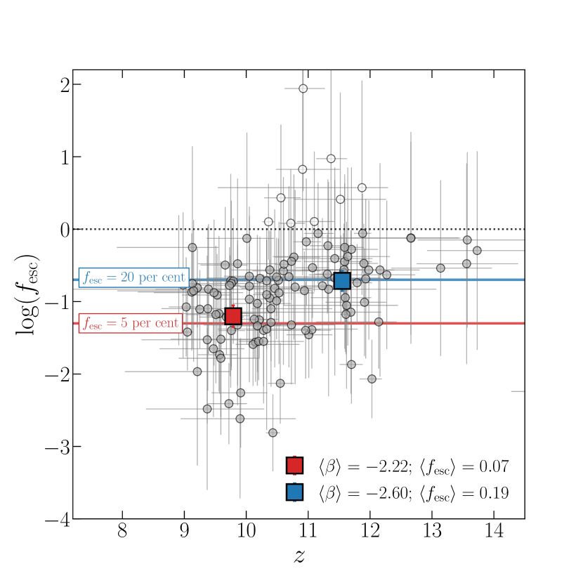
Using a sample galaxies at with direct LyC measurements from HST/COS spectroscopy, Chisholm et al. (2022) presented a strong () correlation between and . The majority of the sample ( galaxies) was drawn from the Low-redshift Lyman Continuum Survey (LzLCS; Flury et al., 2022) which was designed to investigate LyC escape in analogues of young high redshift galaxies. Interestingly, the bluest objects in this sample have . The result of applying the Chisholm et al. (2022) relation (their equation 18) to our data is shown in Fig. 11. While the scatter for individual objects is substantial, the population average values yield robust constraints. Using the fitted values of from Fig. 5, the Chisholm et al. (2022) relation yeilds average values of at to at .
Interestingly, if , then the galaxy population that has already been observed with JWST is likely providing enough ionizing photons to drive reionization at . In Fig. 12 we demonstrate this by showing the emission rate of ionizing photons into the IGM per comoving Mpc3 () as a function of the integration limit of the UV luminosity function. The calculations assume and the UV LF of McLeod et al. (2023). We calculate for three values of (i.e. the production efficiency of LyC photons in units of ) that bracket the typical range of values inferred for young, low-metallicity galaxies at high redshifts (i.e. ; e.g. Bouwens et al., 2016; Atek et al., 2023; Tang et al., 2019; Tang et al., 2023). The ionizing photon output needed to maintain an ionized IGM fraction of is given by the prescription of Madau et al. (1999):
| (5) |
where is the IGM clumping factor which we set following the prescription of Shull et al. (2012).
Setting in equation 5 represents the limiting case of maintaining a fully ionized Universe at redshift . However, at the Universe is expected to be only partially ionized. Models assuming an early and slow reionization typically have (e.g. Finkelstein et al., 2019) while late and rapid models have (e.g. Naidu et al., 2020). It can be seen from Fig. 12 that, based on the above assumptions, the currently-observed galaxy population (i.e. ) is likely providing enough ionizing photons to maintain . Accounting for the population of fainter galaxies, examples of which have been uncovered down to (e.g. Atek et al., 2023), implies that the full galaxy population could in principle be supplying a sufficient number photons to maintain an ionization fraction of per cent at . Certainly, the large abundance of blue galaxies at unveiled by early JWST studies would appear disfavour low ionized IGM fractions of per cent.
5 Summary and Conclusions
We have measured the rest-frame ultraviolet (UV) continuum slopes () for a sample of galaxy candidates at . The majority of these candidates ( per cent) are drawn from our new wide-area JWST sample (Section 2.1). This new sample has enabled us to improve upon our previous work (Cullen et al., 2023) in terms of sample size, on-sky area covered and median imaging depth. Using a robust power-law fitting technique validated against available spectroscopy (Section 2.3), we report precise estimates of at . The main aim of this analysis is to use the average values of for these galaxies to place constraints on the typical dust obscuration experienced at the earliest cosmic epochs. Our main results can be summarized as follows:
-
1.
We measure an inverse-variance weighted mean value of for our full primary wide-area sample at . Incorporating the candidates from Cullen et al. (2023) which includes UV-bright ground-based COSMOS/UltraVISTA sources at lower redshift (with ; Fig. 1) yields a slightly redder value of at a lower average redshift of . Uniformly, therefore, our sample displays blue UV continuum slopes indicative of dust-poor galaxies at these redshifts. However, a value of is not inconsistent with moderate amounts of dust attenuation, nor more extreme than blue objects observed in the local Universe (e.g. NGC 1705; ).
-
2.
Although the full sample median value is , we find evidence for a steep trend in our primary wide-area sample between and (Fig. 4). The average value of evolves from at to at . This represents a rapid evolution of over Myr of cosmic time. In the highest redshift bin, the average UV continuum slope is consistent with pure stellar plus nebular continuum emission in the absence of dust (Fig. 9).
-
3.
Fitting a step function model to the data we find that the galaxy population is becoming uniformly extremely blue at (Fig. 5). Below this transition redshift, our sample displays while at the typical value is . This ’dust-free’ value of represents the extreme blue end of any objects observed at low redshift (e.g. Chisholm et al., 2022), but is the average value of our sample at . Our results suggest that galaxies at contain negligible amounts of dust.
-
4.
In the redshift range we utilise the large dynamic range in enabled by the inclusion of COSMOS/UltraVISTA candidates to investigate the relationship between and absolute UV magnitude (). We find evidence for a relation such that brighter galaxies display redder UV slopes (Fig. 7). This is consistent with a picture in which the brighter (and more massive) galaxies at are more dust obscured. Fitting the at these redshifts, we find ; this slope is consistent with values derived a lower redshifts (down to ; e.g. Bouwens et al., 2014). Our results therefore suggest that a relation has been in place since with a slope that is not strongly evolving with redshift. However, the normalisation of the relation is clearly evolving, with at compared to at . At fixed , galaxies are less dust (and metal) enriched at earlier cosmic epochs.
-
5.
At our data are not sufficient to constrain the relation due to a lack galaxies with (Fig. 7). However, the data at these redshifts remain consistent with a relatively shallow slope and a continued evolution to bluer values of . Our results suggest that the normalisation evolves from at to at . At , wider-area surveys are required improve the dynamic range and accurately constrain the relation.
The primary new result of this work is the evolution towards an extremely dust-poor, perhaps even dust-free, galaxy population by , with average UV continuum slopes of . Similarly blue UV slopes at these redshifts have also been reported in other independent analyses (Austin et al., 2023; Topping et al., 2022; Morales et al., 2023). Competing theoretical explanations for dust-free galaxies exist, but these different physical processes cannot be discriminated with our current data. Nevertheless, these results place important constraints on the origin of dust and metals in the first galaxies. Furthermore, our results imply that the ISM conditions in galaxies at favour a significant escape fraction of ionizing photons, and that the already-observed population of galaxies at these redshifts (i.e. with ) is likely capable of maintaining ionized IGM fractions of per cent.
Acknowledgements
F. Cullen, K. Z. Arellano-Cordova and T. M. Stanton acknowledge support from a UKRI Frontier Research Guarantee Grant (PI Cullen; grant reference EP/X021025/1). R. J. McLure, D. J. McLeod, J. S. Dunlop, C. Donnan, R. Begley and M. L. Hamadouche, acknowledge the support of the Science and Technology Facilities Council. A. C. Carnall thanks the Leverhulme Trust for their support via a Leverhulme Early Career Fellowship. R. A. A. Bowler acknowledges support from an STFC Ernest Rutherford Fellowship (grant number ST/T003596/1). J. S. Dunlop also acknowledges the support of the Royal Society via a Royal Society Research Professorship.
Some of the data products presented herein were retrieved from the Dawn JWST Archive (DJA). DJA is an initiative of the Cosmic Dawn Center, which is funded by the Danish National Research Foundation under grant No. 140. This work is based on observations collected at the European Southern Observatory under ESO programme ID 179.A-2005 and 198.A-2003 and on data products produced by CALET and the Cambridge Astronomy Survey Unit on behalf of the UltraVISTA consortium. For the purpose of open access, the author has applied a Creative Commons Attribution (CC BY) licence to any Author Accepted Manuscript version arising from this submission. We would like to thank Andrea Ferrara, Gergö Popping and Ken Duncan for useful suggestions and feedback.
Data Availability
All JWST and HST data products are available via the Mikulski Archive for Space Telescopes (https://mast.stsci.edu). UltraVISTA DR5 data are available through the ESO portal (http://archive.eso.org/scienceportal/home?data_collection=UltraVISTA&publ_date=2023-05-03). Additional data products are available from the authors upon reasonable request.
References
- Arnouts & Ilbert (2011) Arnouts S., Ilbert O., 2011, LePHARE: Photometric Analysis for Redshift Estimate (ascl:1108.009)
- Arrabal Haro et al. (2023a) Arrabal Haro P., et al., 2023a, arXiv e-prints, p. arXiv:2303.15431
- Arrabal Haro et al. (2023b) Arrabal Haro P., et al., 2023b, ApJ, 951, L22
- Atek et al. (2023) Atek H., et al., 2023, arXiv e-prints, p. arXiv:2308.08540
- Austin et al. (2023) Austin D., et al., 2023, ApJ, 952, L7
- Bagley et al. (2023) Bagley M. B., et al., 2023, arXiv e-prints, p. arXiv:2302.05466
- Bakx et al. (2023) Bakx T. J. L. C., et al., 2023, MNRAS, 519, 5076
- Begley et al. (2022) Begley R., et al., 2022, MNRAS, 513, 3510
- Bertin & Arnouts (1996) Bertin E., Arnouts S., 1996, A&AS, 117, 393
- Bezanson et al. (2022) Bezanson R., et al., 2022, arXiv e-prints, p. arXiv:2212.04026
- Bhatawdekar & Conselice (2021) Bhatawdekar R., Conselice C. J., 2021, ApJ, 909, 144
- Bouwens et al. (2009) Bouwens R. J., et al., 2009, ApJ, 705, 936
- Bouwens et al. (2010) Bouwens R. J., et al., 2010, ApJ, 708, L69
- Bouwens et al. (2012) Bouwens R. J., et al., 2012, ApJ, 754, 83
- Bouwens et al. (2014) Bouwens R. J., et al., 2014, ApJ, 793, 115
- Bouwens et al. (2016) Bouwens R. J., Smit R., Labbé I., Franx M., Caruana J., Oesch P., Stefanon M., Rasappu N., 2016, ApJ, 831, 176
- Bowler et al. (2023) Bowler R. A. A., et al., 2023, arXiv e-prints, p. arXiv:2309.17386
- Brammer (2022) Brammer G., 2022, msaexp: NIRSpec analyis tools, doi:10.5281/zenodo.7313329, https://doi.org/10.5281/zenodo.7313329
- Brammer (2023) Brammer G., 2023, grizli, doi:10.5281/zenodo.8210732, https://doi.org/10.5281/zenodo.8210732
- Brammer et al. (2008) Brammer G. B., van Dokkum P. G., Coppi P., 2008, ApJ, 686, 1503
- Bruzual & Charlot (2003) Bruzual G., Charlot S., 2003, MNRAS, 344, 1000
- Bunker et al. (2023) Bunker A. J., et al., 2023, arXiv e-prints, p. arXiv:2302.07256
- Byler et al. (2017) Byler N., Dalcanton J. J., Conroy C., Johnson B. D., 2017, ApJ, 840, 44
- Byrne et al. (2022) Byrne C. M., Stanway E. R., Eldridge J. J., McSwiney L., Townsend O. T., 2022, MNRAS, 512, 5329
- Calzetti et al. (1994) Calzetti D., Kinney A. L., Storchi-Bergmann T., 1994, ApJ, 429, 582
- Calzetti et al. (2000) Calzetti D., Armus L., Bohlin R. C., Kinney A. L., Koornneef J., Storchi-Bergmann T., 2000, ApJ, 533, 682
- Caminha et al. (2019) Caminha G. B., et al., 2019, A&A, 632, A36
- Casey et al. (2023) Casey C. M., et al., 2023, ApJ, 954, 31
- Castellano et al. (2023) Castellano M., et al., 2023, ApJ, 948, L14
- Chabrier (2003) Chabrier G., 2003, PASP, 115, 763
- Chisholm et al. (2022) Chisholm J., et al., 2022, MNRAS, 517, 5104
- Coe et al. (2019) Coe D., et al., 2019, ApJ, 884, 85
- Conroy & Gunn (2010) Conroy C., Gunn J. E., 2010, ApJ, 712, 833
- Conroy et al. (2009) Conroy C., Gunn J. E., White M., 2009, ApJ, 699, 486
- Cullen et al. (2017) Cullen F., McLure R. J., Khochfar S., Dunlop J. S., Dalla Vecchia C., 2017, MNRAS, 470, 3006
- Cullen et al. (2023) Cullen F., et al., 2023, MNRAS, 520, 14
- Curtis-Lake et al. (2023) Curtis-Lake E., et al., 2023, Nature Astronomy, 7, 622
- Dekel et al. (2023) Dekel A., Sarkar K. C., Birnboim Y., Mandelker N., Li Z., 2023, MNRAS, 523, 3201
- Donnan et al. (2023a) Donnan C. T., et al., 2023a, MNRAS, 518, 6011
- Donnan et al. (2023b) Donnan C. T., McLeod D. J., McLure R. J., Dunlop J. S., Carnall A. C., Cullen F., Magee D., 2023b, MNRAS, 520, 4554
- Dunlop et al. (2012) Dunlop J. S., McLure R. J., Robertson B. E., Ellis R. S., Stark D. P., Cirasuolo M., de Ravel L., 2012, MNRAS, 420, 901
- Dunlop et al. (2013) Dunlop J. S., et al., 2013, MNRAS, 432, 3520
- Eisenstein et al. (2023) Eisenstein D. J., et al., 2023, arXiv e-prints, p. arXiv:2306.02465
- Ellis et al. (2013) Ellis R. S., et al., 2013, ApJ, 763, L7
- Esmerian & Gnedin (2023) Esmerian C. J., Gnedin N. Y., 2023, arXiv e-prints, p. arXiv:2308.11723
- Ferland et al. (2017) Ferland G. J., et al., 2017, Rev. Mex. Astron. Astrofis., 53, 385
- Ferrara (2023) Ferrara A., 2023, arXiv e-prints, p. arXiv:2310.12197
- Ferrara et al. (2023) Ferrara A., Pallottini A., Dayal P., 2023, MNRAS, 522, 3986
- Finkelstein et al. (2012) Finkelstein S. L., et al., 2012, ApJ, 756, 164
- Finkelstein et al. (2019) Finkelstein S. L., et al., 2019, ApJ, 879, 36
- Finkelstein et al. (2022) Finkelstein S. L., et al., 2022, arXiv e-prints, p. arXiv:2207.12474
- Flury et al. (2022) Flury S. R., et al., 2022, ApJS, 260, 1
- Franco et al. (2023) Franco M., et al., 2023, arXiv e-prints, p. arXiv:2308.00751
- Fudamoto et al. (2023) Fudamoto Y., et al., 2023, arXiv e-prints, p. arXiv:2309.02493
- Fujimoto et al. (2022) Fujimoto S., et al., 2022, arXiv e-prints, p. arXiv:2211.03896
- Furtak et al. (2023) Furtak L. J., et al., 2023, MNRAS, 523, 4568
- Gordon et al. (2003) Gordon K. D., Clayton G. C., Misselt K. A., Landolt A. U., Wolff M. J., 2003, ApJ, 594, 279
- Götberg et al. (2018) Götberg Y., de Mink S. E., Groh J. H., Kupfer T., Crowther P. A., Zapartas E., Renzo M., 2018, A&A, 615, A78
- Hainline et al. (2023) Hainline K. N., et al., 2023, arXiv e-prints, p. arXiv:2306.02468
- Harikane et al. (2023a) Harikane Y., Nakajima K., Ouchi M., Umeda H., Isobe Y., Ono Y., Xu Y., Zhang Y., 2023a, arXiv e-prints, p. arXiv:2304.06658
- Harikane et al. (2023b) Harikane Y., et al., 2023b, ApJS, 265, 5
- Heintz et al. (2023) Heintz K. E., et al., 2023, arXiv e-prints, p. arXiv:2306.00647
- Illingworth et al. (2013) Illingworth G. D., et al., 2013, ApJS, 209, 6
- Illingworth et al. (2016) Illingworth G., et al., 2016, arXiv e-prints, p. arXiv:1606.00841
- Inayoshi et al. (2022) Inayoshi K., Harikane Y., Inoue A. K., Li W., Ho L. C., 2022, ApJ, 938, L10
- Inoue et al. (2014) Inoue A. K., Shimizu I., Iwata I., Tanaka M., 2014, MNRAS, 442, 1805
- Jaacks et al. (2018) Jaacks J., Finkelstein S. L., Bromm V., 2018, MNRAS, 475, 3883
- Johnson et al. (2023) Johnson B., et al., 2023, dfm/python-fsps: v0.4.4, Zenodo, doi:10.5281/zenodo.8230430
- Kannan et al. (2022) Kannan R., Smith A., Garaldi E., Shen X., Vogelsberger M., Pakmor R., Springel V., Hernquist L., 2022, MNRAS, 514, 3857
- Keating et al. (2023) Keating L. C., Bolton J. S., Cullen F., Haehnelt M. G., Puchwein E., Kulkarni G., 2023, arXiv e-prints, p. arXiv:2308.05800
- Kirchschlager et al. (2022) Kirchschlager F., Mattsson L., Gent F. A., 2022, MNRAS, 509, 3218
- Kneib et al. (2011) Kneib J.-P., Bonnet H., Golse G., Sand D., Jullo E., Marshall P., 2011, LENSTOOL: A Gravitational Lensing Software for Modeling Mass Distribution of Galaxies and Clusters (strong and weak regime), Astrophysics Source Code Library, record ascl:1102.004 (ascl:1102.004)
- Koekemoer et al. (2011) Koekemoer A. M., et al., 2011, ApJS, 197, 36
- Leitherer et al. (1999) Leitherer C., et al., 1999, ApJS, 123, 3
- Lotz et al. (2017) Lotz J. M., et al., 2017, ApJ, 837, 97
- Madau (1995) Madau P., 1995, ApJ, 441, 18
- Madau et al. (1999) Madau P., Haardt F., Rees M. J., 1999, ApJ, 514, 648
- Mason et al. (2015) Mason C. A., Trenti M., Treu T., 2015, ApJ, 813, 21
- Mason et al. (2023) Mason C. A., Trenti M., Treu T., 2023, MNRAS, 521, 497
- Matthee et al. (2017) Matthee J., Sobral D., Best P., Khostovan A. A., Oteo I., Bouwens R., Röttgering H., 2017, MNRAS, 465, 3637
- McLeod et al. (2023) McLeod D. J., et al., 2023, arXiv e-prints, p. arXiv:2304.14469
- McLure et al. (2018) McLure R. J., et al., 2018, MNRAS, 476, 3991
- Meurer et al. (1999) Meurer G. R., Heckman T. M., Calzetti D., 1999, ApJ, 521, 64
- Miralda-Escudé (1998) Miralda-Escudé J., 1998, ApJ, 501, 15
- Morales et al. (2023) Morales A. M., et al., 2023, arXiv e-prints, p. arXiv:2311.04294
- Naidu et al. (2020) Naidu R. P., Tacchella S., Mason C. A., Bose S., Oesch P. A., Conroy C., 2020, ApJ, 892, 109
- Naidu et al. (2022) Naidu R. P., et al., 2022, arXiv e-prints, p. arXiv:2207.09434
- Nanayakkara et al. (2023) Nanayakkara T., et al., 2023, ApJ, 947, L26
- Nath et al. (2023) Nath B. B., Vasiliev E. O., Drozdov S. A., Shchekinov Y. A., 2023, MNRAS, 521, 662
- Oesch et al. (2016) Oesch P. A., et al., 2016, ApJ, 819, 129
- Oguri (2010) Oguri M., 2010, glafic: Software Package for Analyzing Gravitational Lensing, Astrophysics Source Code Library, record ascl:1010.012 (ascl:1010.012)
- Oke (1974) Oke J. B., 1974, ApJS, 27, 21
- Oke & Gunn (1983) Oke J. B., Gunn J. E., 1983, ApJ, 266, 713
- Pascale et al. (2022) Pascale M., et al., 2022, ApJ, 938, L6
- Pontoppidan et al. (2022) Pontoppidan K., et al., 2022, arXiv e-prints, p. arXiv:2207.13067
- Popping (2023) Popping G., 2023, A&A, 669, L8
- Postman et al. (2012) Postman M., et al., 2012, ApJS, 199, 25
- Reddy et al. (2018) Reddy N. A., et al., 2018, ApJ, 853, 56
- Rieke & the JADES Collaboration (2023) Rieke M., the JADES Collaboration 2023, arXiv e-prints, p. arXiv:2306.02466
- Robertson et al. (2010) Robertson B. E., Ellis R. S., Dunlop J. S., McLure R. J., Stark D. P., 2010, Nature, 468, 49
- Robertson et al. (2023) Robertson B. E., et al., 2023, Nature Astronomy, 7, 611
- Rogers et al. (2013) Rogers A. B., McLure R. J., Dunlop J. S., 2013, MNRAS, 429, 2456
- Rogers et al. (2014) Rogers A. B., et al., 2014, MNRAS, 440, 3714
- Sanders et al. (2023) Sanders R. L., Shapley A. E., Topping M. W., Reddy N. A., Brammer G. B., 2023, ApJ, 955, 54
- Shen et al. (2023) Shen X., Vogelsberger M., Boylan-Kolchin M., Tacchella S., Kannan R., 2023, MNRAS, 525, 3254
- Shull et al. (2012) Shull J. M., Harness A., Trenti M., Smith B. D., 2012, ApJ, 747, 100
- Speagle (2020) Speagle J. S., 2020, MNRAS, 493, 3132
- Stanway et al. (2016) Stanway E. R., Eldridge J. J., Becker G. D., 2016, MNRAS, 456, 485
- Steidel et al. (2016) Steidel C. C., Strom A. L., Pettini M., Rudie G. C., Reddy N. A., Trainor R. F., 2016, ApJ, 826, 159
- Tacchella et al. (2018) Tacchella S., Bose S., Conroy C., Eisenstein D. J., Johnson B. D., 2018, ApJ, 868, 92
- Tacchella et al. (2022) Tacchella S., et al., 2022, ApJ, 927, 170
- Tang et al. (2019) Tang M., Stark D. P., Chevallard J., Charlot S., 2019, MNRAS, 489, 2572
- Tang et al. (2023) Tang M., et al., 2023, MNRAS, 526, 1657
- Tanvir et al. (2019) Tanvir N. R., et al., 2019, MNRAS, 483, 5380
- Todini & Ferrara (2001) Todini P., Ferrara A., 2001, MNRAS, 325, 726
- Topping et al. (2022) Topping M. W., Stark D. P., Endsley R., Plat A., Whitler L., Chen Z., Charlot S., 2022, ApJ, 941, 153
- Topping et al. (2023) Topping M. W., et al., 2023, arXiv e-prints, p. arXiv:2307.08835
- Treu et al. (2022) Treu T., et al., 2022, arXiv e-prints, p. arXiv:2206.07978
- Umeda et al. (2023) Umeda H., Ouchi M., Nakajima K., Harikane Y., Ono Y., Xu Y., Isobe Y., Zhang Y., 2023, arXiv e-prints, p. arXiv:2306.00487
- Valentino et al. (2023) Valentino F., et al., 2023, ApJ, 947, 20
- Vázquez et al. (2004) Vázquez G. A., Leitherer C., Heckman T. M., Lennon D. J., de Mello D. F., Meurer G. R., Martin C. L., 2004, ApJ, 600, 162
- Vijayan et al. (2021) Vijayan A. P., Lovell C. C., Wilkins S. M., Thomas P. A., Barnes D. J., Irodotou D., Kuusisto J., Roper W. J., 2021, MNRAS, 501, 3289
- Wang et al. (2020) Wang X., et al., 2020, in American Astronomical Society Meeting Abstracts #235. p. 426.03
- Whitaker et al. (2019) Whitaker K. E., et al., 2019, ApJS, 244, 16
- Wilkins et al. (2016) Wilkins S. M., Bouwens R. J., Oesch P. A., Labbé I., Sargent M., Caruana J., Wardlow J., Clay S., 2016, MNRAS, 455, 659
- Williams et al. (2023) Williams C. C., et al., 2023, arXiv e-prints, p. arXiv:2301.09780
- Windhorst et al. (2023) Windhorst R. A., et al., 2023, AJ, 165, 13
- Yoon et al. (2023) Yoon I., et al., 2023, ApJ, 950, 61
- Yung et al. (2019) Yung L. Y. A., Somerville R. S., Finkelstein S. L., Popping G., Davé R., 2019, MNRAS, 483, 2983
- Yung et al. (2023) Yung L. Y. A., Somerville R. S., Finkelstein S. L., Wilkins S. M., Gardner J. P., 2023, arXiv e-prints, p. arXiv:2304.04348
- Ziparo et al. (2023) Ziparo F., Ferrara A., Sommovigo L., Kohandel M., 2023, MNRAS, 520, 2445
- Zitrin et al. (2015) Zitrin A., et al., 2015, ApJ, 801, 44
| Field | ID | PI | Reference | Ancillary Data | Lensing Map |
|---|---|---|---|---|---|
| CEERS | 1345 | S. Finkelstein | Finkelstein et al. (2022) | Koekemoer et al. (2011),Wang et al. (2020) | - |
| Quintet | 2732 | K. M. Pontoppidan | Pontoppidan et al. (2022) | - | - |
| Cartwheel | 2727 | K. M. Pontoppidan | Pontoppidan et al. (2022) | - | - |
| SMACS 0723 | 2736 | K. M. Pontoppidan | Pontoppidan et al. (2022) | Coe et al. (2019) | P22 |
| J1235 | 1063 | B. Sunnquist | - | - | - |
| GLASS | 1327 | T. Treu | Treu et al. (2022) | - | F23 |
| A2744-DDT | 2756 | Chen | - | - | F23 |
| UNCOVER | 2561 | I. Labbe | Bezanson et al. (2022) | Lotz et al. (2017) | F23 |
| RXJ 2129 | 2767 | Kelly | - | Postman et al. (2012) | Z15, C19 |
| WHL 0137 | 2282 | D. Coe | - | Coe et al. (2019) | O10, K11, Z15 |
| MACS 0647 | 1433 | D. Coe | - | Postman et al. (2012) | Z15 |
| NEP TDF | 2738 | R. Windhorst | Windhorst et al. (2023) | - | - |
| JEMS | 1963 | C. Williams | Williams et al. (2023) | Illingworth et al. (2016), Whitaker et al. (2019) | - |
| NGDEEP | 2079 | S. Finkelstein, C. Papovich, N. Pirzkal | Bagley et al. (2023) | Illingworth et al. (2016), Whitaker et al. (2019) | - |
| JADES | 1180, 1210 | D. Eisenstein, N. Luetzgendorf | Eisenstein et al. (2023) | Illingworth et al. (2016), Whitaker et al. (2019) | - |
| Field | F435W | F606W | F814W | F090W | F115W | F150W | F200W | F277W | F300M | F356W | F410M | F444W | |
|---|---|---|---|---|---|---|---|---|---|---|---|---|---|
| SMACS 0723 | 26.7 | 27.7 | 26.8 | 28.5 | - | 28.6 | 28.7 | 28.7 | - | 28.7 | - | 28.4 | |
| Quintet | - | - | - | 26.9 | - | 27.0 | 27.3 | 27.7 | - | 27.8 | - | 27.4 | |
| Cartwheel | - | - | - | 27.3 | - | 27.3 | 27.6 | 27.9 | - | 27.9 | - | 27.8 | |
| WHL 0137 | 26.6 | 27.4 | 26.8 | 27.7 | 27.9 | 28.0 | 28.1 | 28.3 | - | 28.2 | 27.9 | 27.9 | |
| MACS 0647 | 26.7 | 27.2 | 27.2 | - | 27.7 | 27.8 | 28.2 | 28.3 | - | 28.3 | - | 28.0 | |
| J1235 | - | - | - | 28.4 | 28.5 | 28.4 | 28.8 | 28.9 | 28.6 | 28.9 | - | 28.3 | |
| NEP TDF | - | - | - | 28.1 | 28.2 | 28.0 | 28.3 | 28.7 | - | 28.5 | 28.1 | 28.3 | |
| RXJ 2129 | 26.8 | 27.2 | 26.7 | - | 27.2 | 27.8 | 27.6 | 27.9 | - | 28.3 | - | 27.7 | |
| GLASS | - | - | - | 28.8 | 28.9 | 28.5 | 28.7 | 28.9 | - | 28.9 | - | 28.8 | |
| DDT 2756 | - | - | - | - | 28.5 | 28.6 | 28.8 | 28.7 | - | 28.9 | - | 28.3 | |
| UNCOVER | 28.2 | 28.6 | 28.4 | - | 28.6 | 28.6 | 28.8 | 28.8 | - | 28.9 | 28.5 | 28.5 | |
| UNCOVER-South | - | - | - | 28.5 | 28.4 | 28.6 | 28.7 | 28.7 | - | 28.8 | 28.1 | 28.5 | |
| CEERS | 27.8 | 28.4 | 28.0 | - | 28.5 | 28.4 | 28.6 | 28.6 | - | 28.5 | 28.0 | 28.2 | |
| NGDEEP | 28.5 | 29.2 | 28.7 | - | 29.2 | 29.2 | 29.2 | 29.5 | - | 29.2 | - | 29.2 | |
| JADES/JEMS | 28.6 | 28.9 | 28.4 | 29.5 | 29.9 | 29.8 | 29.9 | 30.1 | - | 30.0 | 29.5 | 29.7 |
Appendix A Overview of the wide-area JWST sample
In Table 5 we give an overview of the datasets used in this work to construct our wide-area JWST sample. We include the field, proposal ID and PI name of each dataset as well as a references to the relevant survey paper, ancillary data and lensing maps where applicable. In Table 6 we list the global limiting magnitudes for each dataset in each of the observed filters. With the exception of JADES, NGDEEP and UNCOVER-South, which are described in Section 2, the data reduction and catalogue creation for each dataset is described in McLeod et al. (2023). Across these various datasets, which cover a non-contiguous on-sky area of arcmin2, we select galaxy candidates at .
Appendix B Details of the nebular continuum models
In Section 4.1 we discuss the theoretical ‘blue-limit’ for the UV continuum slope of star-forming galaxies using theoretical stellar population models which include the effect of nebular continuum emission. For the starburst99 (Leitherer et al., 1999; Götberg et al., 2018) and bpassv2.3 (Byrne et al., 2022) stellar models, the nebular continuum predictions were generated using Cloudy v17.03 (Ferland et al., 2017). For a stellar population model of a given age and metallicity, the resulting nebular continuum emission was generated assuming a simple plane-parallel geometry. We assumed a constant H ii region electron density of cm-3 and a dimensionless ionization parameter of . These values are typical of star-forming galaxies at (e.g. Steidel et al., 2016) and early spectroscopic observations with JWST have indicated that galaxies up to are characterised by similar parameters (Sanders et al., 2023). However, we note that although and do affect the resulting nebular continuum, the age and metallicity of the underlying stellar population remain the dominant factor.
For the fsps stellar models we generated nebular continuum emission using the python-fsps library (Johnson et al., 2023). The photoionization models underlying these nebular continuum are described in Byler et al. (2017). In python-fsps the electron density is fixed to cm-3 (Byler et al., 2017) and we assume as before. Despite subtle differences in the nebular modelling, the differences relative to starburst99 and bpassv2.3 visible in Fig. 9 are primarily due to differences in the underlying stellar models.