A generic coupling between internal states and activity leads to activation fronts and criticality in active systems

Abstract

We investigate a generic coupling between the particle’s internal state and self-propulsion to study the onset of collective motion. Our analysis reveals such a coupling renders an otherwise non-critical 2-state system, into an effective 3-state system able to display scale-invariant activity avalanches, proving the existence of an intimate connection with critical phenomena. Furthermore, we identify three distinct propagating front regimes, including a selfish regime. The obtained results provide insight into the way collectives distribute, process, and respond to local environmental cues.

Collective motion is observed in a large variety of biological systems; fish schools Lopez et al. (2012), bird flocks Ballerini et al. (2008), and ungulate herds Ginelli et al. (2015); Gómez-Nava et al. (2022) are a few of the countless existing examples Krause and Ruxton (2002); Vicsek and Zafeiris (2012). Despite the fact that collective motion is in general not a continuous process O’brien et al. (1990); Kramer and McLaughlin (2001), and animal groups display repeated transitions from static to moving phases Gómez-Nava et al. (2022) – with the former associated with e.g. resting or feeding phases – most experimental and theoretical studies have focused on the characterization and modeling of groups of constantly moving units Lopez et al. (2012); Ballerini et al. (2008); Vicsek and Zafeiris (2012). Moreover, transitions from static to moving states have been recently shown to also occur in (subcritical) active colloidal systems Liu et al. (2021), which proves that such transitions are observed in both, living and non-living active matter.

A prominent example of such transitions is the onset of collective motion from an initially polarized static group, which remains largely unexplored. One exception is a recent study on the initiation of a Marathon, where boundary displacements set in motion the crowd Bain and Bartolo (2019). In animal groups, on the other hand, collective motion is often triggered by the behavioral shift, from static to moving, of one single individual Pillot et al. (2011); Toulet et al. (2015); Ginelli et al. (2015); Strandburg-Peshkin et al. (2015). The behavioral shift of this first individual can be the result of, for instance, the decision of the individual to search for a new feeding area, or a reaction to a predator attack Kramer and McLaughlin (2001). In general, it is expected that certain features of the behavioral shift of this first individual – e.g. its velocity – encode information about the stimulus that triggered its behavioral change.

Understanding how information spreads in active and animal systems remains an open crucial question. It has been argued Mora and Bialek (2011); Munoz (2018); Klamser and Romanczuk (2021) that biological systems have to operate at criticality to ensure efficient responses and fast information propagation to external perturbations. In the context of animal behavior, evidence of critical behavior was reported in bird flocks Ballerini et al. (2008); Cavagna et al. (2010); Attanasi et al. (2014), fish schools Poel et al. (2022), and sheep herds Ginelli et al. (2015). Information propagation, on the other hand, has been mostly studied, not on active systems, but on static lattices and networks Castellano et al. (2009). Except for the study of epidemic spreading in moving agent systems Peruani and Sibona (2008, 2019); Rodríguez et al. (2019); Forgács et al. (2022); Zhao et al. (2022); Rodríguez et al. (2022), the role of agent motility on a propagation process, despite its relevance, is unknown. One exception is the study of epidemic spreading in moving agent systems Peruani and Sibona (2008, 2019); Rodríguez et al. (2019); Forgács et al. (2022); Zhao et al. (2022); Rodríguez et al. (2022). Moreover, in this models Peruani and Sibona (2008, 2019); Rodríguez et al. (2019); Forgács et al. (2022); Zhao et al. (2022), with the exception of SIS-like active models Levis et al. (2020); Azaïs et al. (2018); Paoluzzi et al. (2020), active agents do not exhibit coupling between the internal states dynamics and the equation of motion of the agents.

Here, we fill this fundamental gap and investigate a generic coupling in which the agent’s internal state controls the agent’s active speed. Specifically, we consider systems in which the state of each agent $i$ is given by its position $x_{i}$ and its behavioral state $q_{i}$ that adopts one of the two possible values: I (inactive) or A (active). Initially, individuals are equally spaced a distance $\Delta_{0}=|x_{i+1}(t=0)-x_{i}(t=0)|$, where, in 1D, $i=1$ and $i=N$ are the leftmost and rightmost agents, respectively, and all individuals are in state I, except for one agent (usually $i=1$) that is in state A (Fig.1(a)-1(c)). For simplicity, here we focus only on one behavioral transition. Given an agent in state I and another one in state A, separated by a distance $|\Delta x|$, we consider the transition:

$$\text{I}+\text{A}\underset{\gamma(|\Delta x|)}{\longrightarrow}2\text{A}\,,$$ (1)

where $\gamma(|\Delta x|)=\alpha\,K(|\Delta x|/d)$ denotes the transition rate, with $\alpha$ a constant rate, $d$ a characteristic length, and $K(\cdot)$ a function. Here, we report results for $K(u)=\text{e}^{-|u|}$, but tested $K(u)=\text{e}^{-u^{2}}$, and step-functions among other functions and obtained same results SI . The internal state $q_{i}$ is generically coupled with the spatial dynamics of the agent by the following equation:

$$\dot{x}_{i}=\text{V}[q_{i}]=\begin{cases}v&\text{if }q_{i}=\text{A}\\ 0&\text{if }q_{i}=\text{I}\end{cases}\,,$$ (2)

where the dot denotes the temporal derivative and $v$ the velocity of active agents. For $v=0$, the model describes the propagation of state A on a lattice such that for $t\to\infty$, all $N$ individuals end up into state $A$ even in the limit of $N\to\infty$. Thus, there is no phase transition or critical behavior when $v=0$ in any dimension. For $v\neq 0$, the simple generic coupling given by Eq. (2) fundamentally changes the physics of the problem. As explained below, different propagating regimes become possible and the system behaves as an effective three-state model, which allows the system to exhibit in two dimensions a phase transition and critical behavior. We observe that the model can be interpreted as follows. The first individual that becomes active picks up a velocity $v$. All subsequent transitions can be associated with a mimetic process: inactive agents adopt, with a certain probability, the velocity of active agents and thus, acquire the first agent velocity. Below, we explain how sensitive the propagation process is to this initial velocity $v$.

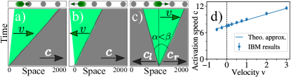
Figure 1: Information propagation in a 1D system. Kymographs show the evolution of the activation wave in simulations; upper panels show the schematic of the system in which active agents are in green and inactive ones are in gray. In panels a and c the activator and all active agents move towards the right, $v>0$, and in b toward the left, $v<0$. The speed of the activation front is given by $c$. In panel c, we have 2 waves traveling with speeds $c_{r}$ and $c_{l}$ to the right and left, respectively, where $c_{r}>c_{l}$. d) Propagating front speed $c$ vs $v$. Blue symbols correspond to simulations, solid line is Eq. (4).

Propagating regimes and fronts.– To understand the presence of distinct propagating regimes and the relation between the propagating front speed $c$ and the active agent velocity $v$, we use a coarse-grained, hydrodynamic description of the model in terms of a density field $\eta_{A}(x,t)=\langle\sum_{i}\delta(x-x_{i}(t))\delta_{q_{i}(t),A}\rangle$ [$\eta_{I}(x,t)=\langle\sum_{i}\delta(x-x_{i}(t))\delta_{q_{i}(t),I}\rangle$] of active [inactive] individuals at time $t$ in position $x$, whose evolution is given by:

$$\partial_{t}\eta_{A}(x,t) =\,\Gamma(x,t)\ \eta_{I}(x,t)-v\ \partial_{x}\eta_{A}(x,t)$$ (3a)

$$\partial_{t}\eta_{I}(x,t) =\text{-}\Gamma(x,t)\ \eta_{I}(x,t)\,,$$ (3b)

where $\Gamma(x,t)=\int_{\text{-}\infty}^{\infty}\eta_{A}(x^{\prime},t)\gamma(|x^{\prime}-x|)dx^{\prime}$. For $v=0$ and after approximating $\Gamma(x,t)\simeq d\alpha\left(a\eta_{A}+\frac{d^{2}b}{2}\partial^{2}_{x}\eta_{A}\right)$, where $a=\int_{\text{-}\infty}^{\infty}K(|u|)du$, and $b=\int_{\text{-}\infty}^{\infty}u^{2}K(|u|)du$, it is possible to show that Eq. (3) exhibits propagating fronts that move at speed $c_{0}\sim\alpha\Delta_{0}^{-1}\sqrt{2\,a\,b}$. In this limit, Eq. (3) exhibits a behavior similar to the one of the Fisher-Kolmogorov-Petrovsky-Piskunov (FKPP) equation Van Saarloos (2003); Fig. (2(a) upper panels). On the other hand, for $v\neq 0$, the behavior of Eq. (3) is fundamentally different from, and not reducible to the one of the FKPP’s equation. When the agent speed is such that $0\!<\!|v|\!<\!c_{0}$, the density profiles of the expanding active population (of a semi-infinite system of agents located initially at $x>0$) can be approximated by a plateau, where the right (R) and left (L) edges are given, respectively, by $y_{R(L)}(x)=A_{R(L)}[1\mp\tanh(x-x_{R(L)}(t))/\ell_{R(L)}]$ with $A_{R(L)}$, $\ell_{R(L)}$ constants. The position of the right and left edges are $x_{R}(t)\propto ct$ and $x_{L}(t)\propto vt$ and thus, advance at speeds $c$ and $v$, respectively; Fig. (2(a) middle panels) SI . In agent-based model (ABM) simulations as well as by integrating Eq. (3), we find that the speed $c$ of the leading edge exhibits a generic linear dependency with the active agent velocity $v$:

$$c(v)\simeq c_{0}+m\,v\,,$$ (4)

where $m>1$. For an exponential function $K$ and in the explored range of $\Delta_{0}$, we obtain $m=\frac{4}{3}$ in both, simulations and from Eq. (3); Fig. 1(d). Note that $c$ depends not only on the agent speed, i.e. $|v|$, but also on the moving direction, i.e. $\text{sgn}(v)$: the propagation is faster when active agents move towards the group than when they do it away from the group (Fig. 1(a)-1(c)).

Another propagation regime – which we refer to as “selfish behavior” – is observed when $v\geq c_{0}$ SI . The initial active agent moves so fast that goes by inactive agents, which do not have the time to transition to the active state and are left behind. Eventually, the fast-moving active agent recruits a second agent that starts running near the initial active agent, which contributes to recruiting a third active agent, and so on, until a collective response emerges; see Fig. (2(a) lower panels). This implies that if we imagine the activation of the first active individual results from a reaction to a predator attack, by moving with velocity $v\geq c_{0}$, this first active individual is able to penetrate inside the group and leave a number of agents between its position and the predator. On the other hand, if the initial active agent chooses to move with $v\ll c_{0}$, the activation propagates over all inactive agents, triggering a collective displacement of the group away from the predator, but where the closest individual to the predator is always the initial active agent.

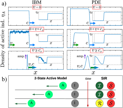
Figure 2: Dynamic regimes. a) Density profile of active agents $\eta_{A}(x,t)$ at a fixed time $t$ in simulations and in the numerical integration of Eq. (3) (PDE). Three different regimes are shown: the limit $v=0$, the slow velocity regime ($0<v<c_{0}$), and the selfish regime ($v\geq c_{0}$). The insets display the density of inactive agents $\eta_{I}(x,t)$ at a fixed time. b) Mapping of our 2-state model with spacial coupling to the 3-state SIR model (color code as in Fig. 1).

From two to effective three-states.– Fluctuations, which cannot be analyzed by the deterministic approach given by Eq. (3) – play a fundamental role in the dynamics of the system [Eqs. (1) and (2)]. To understand such fluctuations, we start out by considering a system composed of only two individuals initially in state $A$ and $I$ located at positions $x_{A}(t)=-v\,t-\Delta_{0}$, with $v\geq 0$, and $x_{I}(t)=0$, respectively. We are interested in knowing the probability $p_{I}(t)$ that the initial inactive individual remains in state $I$ at time $t$. This probability obeys $\partial_{t}p_{I}=-\alpha\,K(|x_{A}(t)|/d)p_{I}$, with initial condition $p_{I}(t=0)=1$. The solution of this equation, with $K(u)=\exp(-u)$, reads:

$$p_{I}(t)=\exp{\!\left[-\frac{\alpha\,\,e^{-\Delta_{0}/d}}{\left(v/d\right)}\left(1-e^{-\frac{v}{d}t}\right)\right]}\,.$$ (5)

For $v\to 0$, it is evident that $p_{I}(t\to\infty)\to 0$, meaning that certainly, the activation of the initially inactive agent has occurred. On the other hand, for a finite $v\neq 0$, $p_{I}(t\to\infty)>0$. This implies that with probability $p_{T}=1-p_{I}(t\to\infty)<1$ the activation of the initially inactive agent has occurred. We observe that this is reminiscent of what happens in the susceptible-infected-recovered (SIR) model or Forest Fire model Kermack and McKendrick (1927); Pastor-Satorras et al. (2015); Bak et al. (1990). The SIR model is defined by the reactions $\mathcal{S}+\mathcal{I}\overset{\sigma}{\rightarrow}2\mathcal{I}$ and $\mathcal{I}\overset{\rho}{\rightarrow}\mathcal{R}$. In a system with only two agents, initially in states $\mathcal{S}$ and $\mathcal{I}$, the probability of finding the initially susceptible agent in state $\mathcal{S}$ at time $t$ reads: $p_{\mathcal{S}}(t)=\exp{\big{[}\text{-}\frac{\sigma}{\rho}\big{(}1-e^{\text{-}\rho t}\big{)}\big{]}}$. Note that $p_{\mathcal{S}}(t)$ displays the same functional form of the probability given by Eq. (5). In the SIR model, if the agent in state $\mathcal{I}$ transitions to $\mathcal{R}$ before passing over the disease, the agent in state $\mathcal{S}$ will never transition, and $p_{\mathcal{S}}(t\to\infty)=\exp{\big{[}\text{-}\frac{\sigma}{\rho}\big{]}}$. Thus, we can map our initial problem with two internal states onto a known excitable model with three states, after realizing that $|v|/d$ plays the role of $\rho$ in the SIR model, Fig. 2(b). Let us consider a one-dimensional semi-infinite system, where for simplicity we assume that each individual interacts with its nearest neighbor to the left and to the right (except for $i=1$). We use the fact that $p_{T}<1$ to analyze the activation propagation. It is evident that if the latest activated agent fails to transmit the activation to its neighbor to the right, the propagation will cease. Let us call $s=n_{A}(t\to\infty)$ the number of active agents at $t\to\infty$ and compute the probability $P(s)$ of observing a “cascade” of size $s$. This requires $s$ successive activation transmissions, followed by a transmission failure, and thus, $P(s)\!=\!\left[p_{T}\right]^{s}\!p_{I}(t\to\infty)\simeq\!e^{-sp_{I}(t\!\rightarrow\!\infty)}p_{I}(t\!\rightarrow\!\infty)$, which leads to $\langle s\rangle\sim 1/p_{I}(t\rightarrow\infty)$. Furthermore, the ratio $\phi=\langle s\rangle/N$ that is our order parameter is such that in 1D, $\lim_{N\to\infty}\phi\to 0$. This implies that infinite-size avalanches cannot occur and the propagation of the activations gets necessarily extinguished with $\langle s\rangle=\langle n_{A}(t\to\infty)\rangle$ remaining finite independently of the system size $N$.

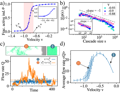
Figure 3: Criticality in the 2D system. a) The order parameter $\phi$ vs $v$. Colored region indicates the area with high variability of possible outcomes ($v_{1}^{*}<v<v_{2}^{*}$). b) Probability $p(s)$ of observing a cascade of size $s=n_{A}(t\to\infty)$ for some velocity values in the specified region of a. Initial condition in a-d corresponds to a column of active agents, while insets in a and b to one initiator. c) Flow rate $Q$ of individuals, crossing $x=0$, as function of time for two representative velocity values, I: $v=-0.1$, II: $v=-0.82$. Small panels above illustrate the simulation snapshots corresponding to the lower panel (color code as in Fig. 1). d) Average flow rate $\langle Q\rangle$ as function of velocity $v$.

Phase transition and criticality.– Since the 3-state SIR model in 2D exhibits critical behavior Grassberger (1983), we investigate whether the 2-state active model in 2D (with effective 3-states) also displays criticality. In 2D, agents move according to $\dot{\mathbf{x}}_{i}=\text{V}[q_{i}]\hat{x}$, while transitions are controlled as before by Eq. (1). We also investigated a model where active agents perform Vicsek-like flocking dynamics obtaining qualitatively the same results, see SI for details and a video. Similar to 1D, at $t=0$ agents are arranged equally spaced on the half-plane that extends to the right, and either there is only one active agent or the entire left boundary is active. Note that the mapping onto the two-dimensional SIR lattice model is no longer exact, but an approximation.

We observe that in 2D the order parameter $\phi$ as function of $v$ indicates the presence of a non-equilibrium phase transition; see Fig. 3(a). For $v<v_{1}^{*}$, the propagation of the active state does not occur, while for $v>v_{2}^{*}$ an infinite propagation is possible. Interestingly, we observe that there exists a range of $v$ values for which there exists a remarkably large variability of possible outcomes for the same initial conditions ($v_{1}^{*}<v<v_{2}^{*}$) SI . Specifically, the distribution of avalanche sizes $P(s)$ is power-law – indicative of critical behavior – with $P(s)\propto s^{-\beta}$ where $\beta$ around $-1$, and thus we observe from small to giant, system spanning activity avalanches; Fig. 3(b). This behavior translates into a spatio-temporal dynamics in which the flow rate $Q(t)$ of active agents crossing at $x=0$ to the left half-plane fluctuates over time around a well-defined mean value for small enough values of $|v|$, while it displays large temporal fluctuations before the system falls into the absorbing phase; Fig. 3(c). Fluctuations are evident by looking at snapshots of the system; upper panels in Fig. 3(c). Note that the average $\langle Q\rangle$ – performed over time, while the system is in the active state – as a function of $v$ exhibits a maximum; Fig. 3(d). This maximum results from the competition of high flows related to large $|v|$ values and larger temporal fluctuations in the flow.

In the dynamical percolation transition in 2D, e.g. SIR model Grassberger (1983), critical behavior is observed only at the critical point. Here, however, we do not need to fine-tune the value of $v$ to obtain a power-law distribution of cascade sizes; these are observed over a large range of $v$ values. This observation, together with the measured exponents of $p(s)$, leaves open the possibility of self-organized critical (SOC) behavior; recall the well-established connection between SOC and systems with absorbing states Munoz et al. (1999). Nevertheless, a detailed numerical investigation, exceeding our current computational capacity, and/or a renormalization group approach, beyond the scope of the current study, is required to settle this very interesting issue.

In short, this study proves that a simple, generic coupling between the agent’s internal state and activity has a profound impact on the physics of the propagation process: the coupling renders an otherwise non-critical 2-state system, into an effective 3-state (excitable) active system able to display critical behavior in 2D. Moreover, the obtained results are of key importance to understanding how collectives distribute, process, and respond to the environmental information that is sensed by group members. Specifically, the analysis shows how the agent velocity – i.e. the velocity chosen by the very first active agent – selects the propagation regime. For example, when individuals move with velocity $0\!<\!v\!\ll\!c_{0}$, e.g. to visit a new feeding area, all group members get activated and move together keeping (on average) the same relative position. On the other hand, if the first individual reacts to a threat, e.g. a predator, it can choose to move with velocity $v\gg c_{0}$ to seek cover inside the collective and leave a number of conspecifics between its position and the predator; cf. Hamilton’s selfish herd hypothesis Hamilton (1971). altering the relative position of individuals within the group requires high-speed values. Finally, these predictions can be tested in experiments of large groups of gregarious animals by characterizing group responses to predatory attacks, e.g. Sosna et al. (2019), where we expect (i) the emergence of activation propagating fronts and (ii) critical behavior, resulting from the here-proposed coupling.

References

- Lopez et al. (2012) U. Lopez, J. Gautrais, I. D. Couzin, and G. Theraulaz, Interface focus 2, 693 (2012).
- Ballerini et al. (2008) M. Ballerini, N. Cabibbo, R. Candelier, A. Cavagna, E. Cisbani, I. Giardina, V. Lecomte, A. Orlandi, G. Parisi, A. Procaccini, et al., Proc. Natl. Acad. Sci. U.S.A. 105, 1232 (2008).
- Ginelli et al. (2015) F. Ginelli, F. Peruani, M.-H. Pillot, H. Chaté, G. Theraulaz, and R. Bon, Proc. Natl. Acad. Sci. U.S.A. 112, 12729 (2015).
- Gómez-Nava et al. (2022) L. Gómez-Nava, R. Bon, and F. Peruani, Nature Physics 18, 1494 (2022).
- Krause and Ruxton (2002) J. Krause and G. D. Ruxton, Living in groups (Oxford University Press, 2002).
- Vicsek and Zafeiris (2012) T. Vicsek and A. Zafeiris, Physics reports 517, 71 (2012).
- O’brien et al. (1990) W. J. O’brien, H. I. Browman, and B. I. Evans, American Scientist 78, 152 (1990).
- Kramer and McLaughlin (2001) D. L. Kramer and R. L. McLaughlin, American Zoologist 41, 137 (2001).
- Liu et al. (2021) Z. T. Liu, Y. Shi, Y. Zhao, H. Chaté, X.-q. Shi, and T. H. Zhang, Proc. Natl. Acad. Sci. U.S.A. 118, e2104724118 (2021).
- Bain and Bartolo (2019) N. Bain and D. Bartolo, Science 363, 46 (2019).
- Pillot et al. (2011) M.-H. Pillot, J. Gautrais, P. Arrufat, I. D. Couzin, R. Bon, and J.-L. Deneubourg, PloS one 6, e14487 (2011).
- Toulet et al. (2015) S. Toulet, J. Gautrais, R. Bon, and F. Peruani, PloS one 10, e0140188 (2015).
- Strandburg-Peshkin et al. (2015) A. Strandburg-Peshkin, D. R. Farine, I. D. Couzin, and M. C. Crofoot, Science 348, 1358 (2015).
- Mora and Bialek (2011) T. Mora and W. Bialek, J Stat Phys 144, 268 (2011).
- Munoz (2018) M. A. Munoz, Rev. Mod. Phys. 90, 031001 (2018).
- Klamser and Romanczuk (2021) P. P. Klamser and P. Romanczuk, PLoS Comput. Biol. 17, e1008832 (2021).
- Cavagna et al. (2010) A. Cavagna, A. Cimarelli, I. Giardina, G. Parisi, R. Santagati, F. Stefanini, and M. Viale, Proc. Natl. Acad. Sci. U.S.A. 107, 11865 (2010).
- Attanasi et al. (2014) A. Attanasi, A. Cavagna, L. Del Castello, I. Giardina, T. S. Grigera, A. Jelić, S. Melillo, L. Parisi, O. Pohl, E. Shen, et al., Nature physics 10, 691 (2014).
- Poel et al. (2022) W. Poel, B. C. Daniels, M. M. Sosna, C. R. Twomey, S. P. Leblanc, I. D. Couzin, and P. Romanczuk, Science Advances 8, eabm6385 (2022).
- Castellano et al. (2009) C. Castellano, S. Fortunato, and V. Loreto, Rev. Mod. Phys. 81, 591 (2009).
- Peruani and Sibona (2008) F. Peruani and G. J. Sibona, Phys. Rev. Lett. 100, 168103 (2008).
- Peruani and Sibona (2019) F. Peruani and G. J. Sibona, Soft matter 15, 497 (2019).
- Rodríguez et al. (2019) J. P. Rodríguez, F. Ghanbarnejad, and V. M. Eguíluz, Scientific reports 9, 1 (2019).
- Forgács et al. (2022) P. Forgács, A. Libál, C. Reichhardt, N. Hengartner, and C. Reichhardt, Scientific Reports 12, 11229 (2022).
- Zhao et al. (2022) Y. Zhao, C. Huepe, and P. Romanczuk, Scientific reports 12, 2588 (2022).
- Rodríguez et al. (2022) J. P. Rodríguez, M. Paoluzzi, D. Levis, and M. Starnini, Phys. Rev. Res. 4, 043160 (2022).
- Levis et al. (2020) D. Levis, A. Diaz-Guilera, I. Pagonabarraga, and M. Starnini, Phys. Rev. Res. 2, 032056 (2020).
- Azaïs et al. (2018) M. Azaïs, S. Blanco, R. Bon, R. Fournier, M.-H. Pillot, and J. Gautrais, PloS one 13, e0206817 (2018).
- Paoluzzi et al. (2020) M. Paoluzzi, M. Leoni, and M. C. Marchetti, Soft Matter 16, 6317 (2020).
- (30) Supplemental Material at URL_will_be_inserted_by_publisher.
- Van Saarloos (2003) W. Van Saarloos, Physics reports 386, 29 (2003).
- Kermack and McKendrick (1927) W. O. Kermack and A. G. McKendrick, Proceedings of the royal society of london. Series A, Containing papers of a mathematical and physical character 115, 700 (1927).
- Pastor-Satorras et al. (2015) R. Pastor-Satorras, C. Castellano, P. Van Mieghem, and A. Vespignani, Rev. Mod. Phys. 87, 925 (2015).
- Bak et al. (1990) P. Bak, K. Chen, and C. Tang, Physics letters A 147, 297 (1990).
- Grassberger (1983) P. Grassberger, Mathematical Biosciences 63, 157 (1983).
- Munoz et al. (1999) M. A. Munoz, R. Dickman, A. Vespignani, and S. Zapperi, Phys. Rev. E. 59, 6175 (1999).
- Hamilton (1971) W. D. Hamilton, J. Theor. Biol. 31, 295 (1971).
- Sosna et al. (2019) M. M. Sosna, C. R. Twomey, J. Bak-Coleman, W. Poel, B. C. Daniels, P. Romanczuk, and I. D. Couzin, Proc. Natl. Acad. Sci. U.S.A. 116, 20556 (2019).