Abstract

In this work, we introduce a three-step semiparametric methodology for the estimation of production frontiers. We consider a model inspired by the well-known Cobb-Douglas production function, wherein input factors operate multiplicatively within the model. Efficiency in the proposed model is assumed to follow a continuous univariate uniparametric distribution in $(0,1)$, referred to as Matsuoka’s distribution, which is introduced and explored. Following model linearization, the first step of the procedure is to semiparametrically estimate the regression function through a local linear smoother. The second step focuses on the estimation of the efficiency parameter in which the properties of the Matsuoka’s distribution are employed. Finally, we estimate the production frontier through a plug-in methodology. We present a rigorous asymptotic theory related to the proposed three-step estimation, including consistency, and asymptotic normality, and derive rates for the convergences presented. Incidentally, we also introduce and study the Matsuoka’s distribution, deriving its main properties, including quantiles, moments, $\alpha$-expectiles, entropies, and stress-strength reliability, among others. The Matsuoka’s distribution exhibits a versatile array of shapes capable of effectively encapsulating the typical behavior of efficiency within production frontier models. To complement the large sample results obtained, a Monte Carlo simulation study is conducted to assess the finite sample performance of the proposed three-step methodology. An empirical application using a dataset of Danish milk producers is also presented.
Keywords: semiparametric regression; production frontiers; asymptotic theory; log-gamma distribution.
MSC2020: 62E10, 62G08, 62F10.

1 Introduction

In the economic theory of production, characterizing efficiency and estimating it is considered essential for performance benchmarking and productivity analysis. As a consequence, production frontier estimation has been the subject of a wide literature since the seminal work of Farrell, (1957). There are two main approaches to production frontier modeling: the stochastic and the deterministic ones. The frontier is considered a fixed function in both approaches. In the stochastic one, deviations from the frontier are treated as aggregations of both inefficiency and statistical noise, while in the deterministic one, they are attributed solely to inefficiencies. Both approaches have strengths and weaknesses, see for instance Bezat, (2009) or Bogetoft and Otto, (2010). In this work we restrict ourselves to the deterministic approach. Popular methods of deterministic frontier estimation are the Data Envelopment Analysis estimator of Charnes et al., (1978) and the Free Disposal Hull estimator introduced by Deprins et al., (2006), which gained attention among applied researchers because they are constructed under very weak assumptions.

The main contribution of the presented paper is to propose a three-step method to estimate a deterministic production frontier model inspired by the well-known Cobb-Douglas production function, in which input factors enter the model multiplicatively. The model assumes that the efficiency follows a certain distribution (see below) depending on an unknown parameter that requires estimation. After linearization, the idea is to first estimate the regression function semiparametrically using a local linear smoother approach. Next, the parameter related to the efficiency is estimated using a feasible method of moments technique. Finally, a plugin approach is used to obtain the frontier function.

To make estimation possible, we propose a new continuous distribution taking values in $(0,1)$ to model efficiency, which is referred to as Matsuoka’s distribution. The main reason for introducing Matsuoka’s distribution is that its density can be successfully applied to capture commonly observed features displayed by the efficiency in multiplicative production frontier models. We provide a study on the introduced Matsuoka’s distribution, deriving basic properties such as distribution and quantile function, moments, skewness, kurtosis, etc, as well as some more specialized results such as incomplete moments and mean deviations, $\alpha$-expectiles, Sharma-Mittal’s entropy (a generalization of the Shannon, Rényi and Tsallis’ entropy), stress-strength reliability, and others.

In summary, we introduce a deterministic production frontier model where the efficiency is Matsuoka distributed and propose a three-step semiparametric estimation scheme. We provide a rigorous asymptotic theory for the proposed estimation method, including rates of convergence in probability for all estimators involved in the estimation procedure for the model with a single input. The finite sample properties of the proposed three-step scheme are assessed through a Monte Carlo simulation study, considering univariate and bivariate inputs. The usefulness of the proposed model is showcased in an empirical application to Danish milk production.

The paper is organized into three main parts. In Section 2, we introduce Matsuoka’s distribution, derive some of its properties, and discuss some inferential aspects. In Section 3, we present the production frontier model and the proposed three-step estimation method and derive the relevant asymptotic theory. To assess the finite sample properties of the proposed estimator, a Monte Carlo simulation study is performed, whose details are presented in Section 4. Section 5 brings the empirical application while Section 6 concludes the paper.

2 The Matsuoka’s distribution

In this section, we introduce Matsuoka’s distributions. We provide a short review of some related distributions first. Stacy, (1962) introduced a 3-parameter family of positive continuous distributions for which the density function is given by

$$f(y;a,d,c)\coloneqq\frac{c}{a^{d}\Gamma(\frac{d}{c})}y^{d-1}e^{-(\frac{y}{a})^{c}}I(y>0),$$

for $a>0$, a scale parameter, and $d,c>0$ shape parameters, called the generalized Gamma distribution. Particular cases of the generalized Gamma distribution are the gamma family, obtained for $c=1$, the Weibull family ($c=d=2$), the Rayleigh family $(c=d=2)$, the log-normal family ($d/c\to\infty$), and the half-normal family ($c=2$ and $d=1$). Of course, all these particular cases are well-known and have seen many applications. In particular, only considering economic duration models, some applications are found in Diebold and Rudebusch, (1990) (exponential), Lancaster, (1979) (gamma), Favero et al., (1994) (Weibull), and Eckstein and Wolpin, (1995) (Log-normal).

A few years later, Consul and Jain, (1971) studied a particular transformation of the generalized gamma distributed to the unit interval $(0,1)$, which was called in the paper the Log-Gamma distribution. This is not to be confused with other log-gamma distributions introduced later by Hogg and Klugman, (1984) considering a similar method as the log-normal distribution, and the log-gamma distribution obtained by taking the logarithm transform of a gamma distribution (Halliwell,, 2021).

Consul and Jain, (1971) derived some properties of the log-gamma and considered applications of the distribution in the context of certain likelihood ratio tests, where the authors derive asymptotic distributions for such tests. As far as we are concerned, there is very little work done after Consul and Jain, (1971) directly related to its log-gamma distribution. The Matsuoka’s distribution is closely related to Consul and Jain, (1971)’s log-gamma. We say that a random variable $X$ taking values in $(0,1)$ follows a Matsuoka distribution with parameter $p>0$, denoted $X\sim\mathrm{M}(p)$ if its density is given by

$$f_{p}(x)\coloneqq 2\sqrt{\frac{-p^{3}\ln(x)}{\pi}}x^{p-1}I(x\in(0,1)).$$ (1)

It is obvious that (1) is non-negative and integrates 1 over $\mathds{R}$ (see formula 4.269.3 in Gradshteyn and Ryzhik,, 2007).

General properties

Figure 1 illustrates the different shapes that the density function $f_{p}$ can assume depending on the values of the parameter $p$. The graphs suggest that small values for $p$ are associated with right-skewed functions, while large values for $p$ are associated with left-skewed functions. To be more precise, for $p\leq 1$ the density of a M$(p)$ distribution assumes a J-shaped pattern, while for $p>1$ the density is unimodal with mode located at $x=e^{-\frac{1}{2(p-1)}}$ with value $\sqrt{\frac{2p^{3}e^{-1}}{\pi(p-1)}}$.

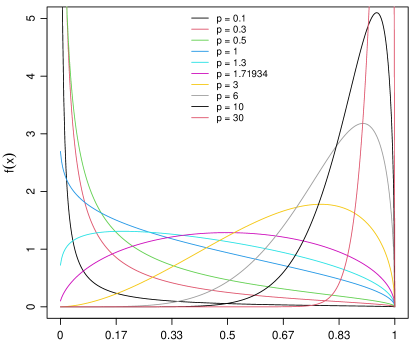
Figure 1: Plot of the density function for various parameters $p$.

Indeed, considering $\ln(f_{p}(x))$, it is easy to see that

$$\frac{\partial\ln(f_{p}(x))}{\partial x}=\frac{2(p-1)\ln(x)+1}{2x\ln(x)}<0,\ \forall x\in(0,1)\qquad\Longleftrightarrow\qquad p\leq 1,$$

so that (1) assumes a J-shape pattern if, and only if, $p\leq 1$. For $p>1$, we have

$$\frac{\partial\ln(f_{p}(x))}{\partial x}=0\qquad\Longleftrightarrow\qquad x=e^{-\frac{1}{2(p-1)}}.$$

Now, the second derivative is given by

$$\frac{\partial^{2}\ln(f_{p}(x))}{\partial x^{2}}=-\frac{2(p-1)\ln(x)^{2}+\ln(x)+1}{2x^{2}\ln^{2}(x)}<0,$$

since, for $p>1$, the polynomial $2(p-1)y^{2}+y+1$ is an upward parabola with complex roots, hence, strictly positive. We conclude that (1) is unimodal for $p>1$ with $x=e^{-\frac{1}{2(p-1)}}$ as mode. In particular, (1) is never symmetric about $1/2$. To see this, observe that, to be symmetric about $1/2$, the mode must be located at $x=1/2$. Hence the only option is $p_{0}=1+\frac{1}{2\ln(2)}$. Also, to be symmetric, (1) must satisfy

$$f_{p_{0}}(x)=f_{p_{0}}(1-x),\ \ \forall x\in(0,1/2)\qquad\Longleftrightarrow\qquad\bigg{(}\frac{x}{1-x}\bigg{)}^{\frac{1}{\ln(2)}}=\frac{\ln(1-x)}{\ln(x)},\ \ \forall x\in(0,1/2),$$

which is, of course, absurd, since the last equality does not hold for any $x\in(0,1/2)$.

To calculate the cumulative distribution function related to (1), $F_{p}(x)$, anti-differentiation based on formula 8.356.4 in Gradshteyn and Ryzhik, (2007) yields

$$F_{p}(x)=\frac{2}{\sqrt{\pi}}\Gamma\bigg{(}\frac{3}{2},-p\ln(x)\bigg{)}I(0<x<1)+I(x\geq 1),$$ (2)

for $x\in\mathds{R}$, where $\Gamma(k,t)=\int_{t}^{\infty}z^{k-1}e^{-z}dz$ for all $k>0$, is the upper incomplete gamma function (see section 8.35 in Gradshteyn and Ryzhik,, 2007). From (2), it is easy to calculate the associated quantile function, which is given by $F^{-1}_{p}(0)=0$, $F^{-1}_{p}(1)=1$ and

$$F^{-1}_{p}(q)=\exp\bigg{\{}\frac{1}{p}\Gamma^{-1}\bigg{(}\frac{3}{2},\frac{q\sqrt{\pi}}{2}\bigg{)}\bigg{\}},$$ (3)

for $q\in(0,1)$, where $\Gamma^{-1}(k,x)$ denotes the inverse of the upper incomplete gamma function, satisfying $\Gamma\big{(}k,\Gamma^{-1}(k,x)\big{)}=\Gamma^{-1}\big{(}k,\Gamma(k,x)\big{)}=x$, for all $x\in\mathds{R}$ and $k>0$. Of course, the upper incomplete gamma function and its inverse can only be computed numerically.

The moments associated with $X\sim\mathrm{M}(p)$ are easily calculated. Upon changing variables to $z=\sqrt{-\ln(t)}\ \Rightarrow\ dt=-2ze^{-(t+p)z^{2}}dz$ and applying integration by parts, it follows that

$$\mathds{E}(X^{k}) =2\sqrt{\frac{p^{3}}{\pi}}\int_{0}^{1}\sqrt{-\ln(t)}t^{p+k-1}dt=\frac{4}{\sqrt{\pi}}\bigg{(}\frac{p}{p+k}\bigg{)}^{\frac{3}{2}}\int_{0}^{\infty}z^{2}e^{-(p+k)z^{2}}dz=\bigg{(}\frac{p}{p+k}\bigg{)}^{\frac{3}{2}},$$ (4)

for all $k>-p$. In particular, from (4) we have,

$$\mathds{E}(X)=\bigg{(}\frac{p}{p+1}\bigg{)}^{\frac{3}{2}},\qquad\mathrm{Var}(X)=\bigg{(}\frac{p}{p+2}\bigg{)}^{\frac{3}{2}}-\bigg{(}\frac{p}{p+1}\bigg{)}^{3},$$

$$\mathds{E}\big{(}[X-\mathds{E}(X)]^{3}\big{)}=\bigg{(}\frac{p}{p+3}\bigg{)}^{\frac{3}{2}}-\frac{3p^{3}}{\big{[}(p+1)(p+2)\big{]}^{\frac{3}{2}}}+2\bigg{(}\frac{p}{p+1}\bigg{)}^{\frac{9}{2}}.$$

The existence of all moments of order $k\in\mathds{N}$ allows the calculation of the moment-generating function as

$$M_{X}(t)=\sum_{n=0}^{\infty}\mathds{E}(X^{n})\frac{t^{n}}{n!}=p^{3/2}\sum_{n=0}^{\infty}\frac{t^{n}}{n!(p+n)^{3/2}}.$$

Observe that the last expression is bounded by $e^{t}$, for all $t\in\mathds{R}$ and $p>0$. Calculating the moment-generating function using (1) seems unfeasible.

Exponential family and MLE

It is easy to see that Matsuoka’s distribution is a member of the 1-parameter regular exponential family, in the form $f_{p}(x)=h(x)\exp\{\eta t(x)-a(\eta)\}$, with canonical parameter $\eta=p$, $a(\eta)=-\frac{3}{2}\ln(\eta)$, $h(x)=-\frac{2\ln(x)}{x\sqrt{\pi}}I(0\leq x\leq 1)$, and natural complete sufficient statistics given by $T(X)=\ln(X)$ (Bickel and Doksum,, 2007, section 1.6). It is easy to show that if $X\sim\mathrm{M}(p)$, then $-\ln(X)\sim\mathrm{Gamma}\big{(}\frac{3}{2},\frac{1}{p}\big{)}$ (in shape/scale parametrization). Let $X_{1},\cdots,X_{n}$ be a sample from $X\sim\mathrm{M}(p)$. The log-likelihood for $p$ is given by

$$\ell(p)=n\ln\biggl{(}\frac{2}{\sqrt{\pi}}\bigg{)}+\frac{3n}{2}\ln(p)+\frac{1}{2}\sum_{i=1}^{n}\ln\bigl{(}-\ln(X_{i})\big{)}+(p-1)\sum_{i=1}^{n}\ln(X_{i}).$$ (5)

Upon deriving (5) with respect to $p$ and equating to 0, the maximum likelihood estimator (MLE) is obtained in closed-form and is given by $\hat{p}=-\frac{3n}{2\sum_{i=1}^{n}\ln(X_{i})}$. Now since $-\ln(X)\sim\mathrm{Gamma}\big{(}\frac{3}{2},\frac{1}{p}\big{)}$, it follows that $-\sum_{i=1}^{n}\ln(X_{i})\sim\mathrm{Gamma}\big{(}\frac{3n}{2},\frac{1}{p}\big{)}$, so that $-\big{[}\sum_{i=1}^{n}\ln(X_{i})\big{]}^{-1}\sim\mbox{Inv-Gamma}\big{(}\frac{3n}{2},p\big{)}$. Hence, we conclude that the MLE is biased with $\mathds{E}(\hat{p})=\big{(}\frac{3n}{3n-2}\big{)}p$. Since the MLE is a function of the complete sufficient statistics $T(\boldsymbol{X})=\sum_{i=1}^{n}\ln(X_{i})$, it follows by the Lehmann-Scheffé theorem that the biased corrected estimator

$$\hat{p}^{\ast}=-\frac{3n-2}{2\sum_{i=1}^{n}\ln(X_{i})}$$

is the uniformly minimum variance unbiased estimator for $p$, with $\mathrm{Var}(\hat{p}^{\ast})=\frac{3p^{2}}{3n-4}$.

Skewness and Kurtosis

Pearson’s moment coefficient of skewness is given by

$$\gamma_{1}\coloneqq\frac{\mathds{E}\left([X-\mu]^{3}\right)}{\mathds{E}\left([X-\mu]^{2}\right)^{\frac{3}{2}}}=\frac{\frac{p^{\frac{3}{2}}}{(p+3)^{\frac{3}{2}}}-\frac{3p^{3}}{\left[(p+1)(p+2)\right]^{\frac{3}{2}}}+\frac{2p^{\frac{9}{2}}}{(p+1)^{\frac{9}{2}}}}{\Big{[}\frac{p^{\frac{3}{2}}}{(p+2)^{\frac{3}{2}}}-\frac{p^{3}}{(p+1)^{3}}\Big{]}^{\frac{3}{2}}},$$

where $\mu=\mathds{E}(X)$. As for the kurtosis, we have

$$\gamma_{2}=\frac{\mathds{E}\big{(}[X-\mu]^{4}\big{)}}{\mathds{E}\big{(}[X-\mu]^{2}\big{)}^{2}}=\frac{\frac{p^{\frac{3}{2}}}{(p+4)^{\frac{3}{2}}}-\frac{4p^{3}}{\left[(p+1)(p+3)\right]^{\frac{3}{2}}}+\frac{6p^{\frac{9}{2}}}{\left[(p+1)(p+2)\right]^{\frac{3}{2}}}-\frac{3p^{6}}{(p+1)^{6}}}{\Big{[}\frac{p^{\frac{3}{2}}}{(p+2)^{\frac{3}{2}}}-\frac{p^{3}}{(p+1)^{3}}\Big{]}^{2}},$$

where the last equality follows upon considering the expanded form of $\mathds{E}\left([X-\mu]^{4}\right)=\mathds{E}(X^{4})-4\mu\mathds{E}(X^{3})+6\mu^{2}\mathds{E}(X^{2})-3\mu^{4}$. Figure 2 shows the behavior of Skewness and Kurtosis of the Matsuoka distribution according to some values of the parameter $p$.

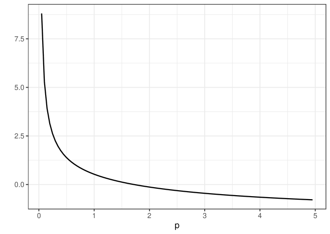
(a) Skewness

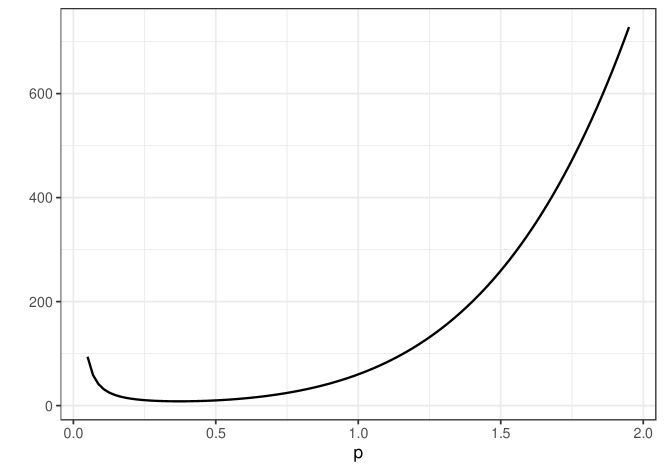
(b) Kurtosis

Figure 2: Skewness and kurtosis.

Incomplete moments and mean deviation

Let $X$ be a random variable with density $f_{X}$. For $y\in\mathds{R}$, the $k$th incomplete moment of $X$ at $y$, denoted by $m_{k}(y)$, is defined as $m_{k}(y)\coloneqq\int_{-\infty}^{y}x^{k}f_{X}(x)dx$. If $X\sim\mathrm{M}(p)$ and $0<y<1$, we have

$$m_{k}(y) =\int_{0}^{y}x^{k}f_{p}(x)dx=\frac{2p^{\frac{3}{2}}}{\sqrt{\pi}}\int_{0}^{y}\sqrt{-\ln(x)}x^{p+k-1}dx$$

$$=\frac{2p^{\frac{3}{2}}}{\pi^{\frac{1}{2}}(p+k)^{\frac{3}{2}}}\Gamma\bigg{(}\frac{3}{2},-(p+k)\ln(y)\bigg{)},$$ (6)

where the integral is computed using anti-differentiation based on 8.356.4 in Gradshteyn and Ryzhik, (2007). From (2), the mean deviations about the mean and the median can be easily computed for a random variable $X$ following Matsuoka’s distribution with parameter $p$ by using the relations

$$\delta_{1}(p)\coloneqq\mathds{E}\big{(}|X-\mu|\big{)}=2\mu F_{p}(\mu)-2m_{1}(\mu),\quad\mbox{and}\quad\delta_{2}(p)\coloneqq\mathds{E}\big{(}|X-M|\big{)}=\mu-2m_{1}(M),$$

where $\mu\coloneqq\mathds{E}(X)$ and $M\coloneqq F_{p}^{-1}(1/2)$.

$\alpha$-expectiles

Given $\alpha\in(0,1)$, for a random variable $X$ with $\mathds{E}(X^{2})<\infty$, the $\alpha$-expectile of $X$, denoted by $\epsilon_{\alpha}(X)$, is defined as

$$\epsilon_{\alpha}(X)\coloneqq\underset{s\in\mathds{R}}{\operatorname*{arg\,min}}\big{\{}(1-\alpha)\mathds{E}\big{(}([X-s]_{-})^{2}\big{)}+\alpha\mathds{E}\big{(}([X-s]_{+})^{2}\big{)}\big{\}},$$

where $[x]_{+}\coloneqq\max\{x,0\}$ and $[x]_{-}\coloneqq-\min\{x,0\}$. Expectiles are often used in regression models as a simpler and more efficient alternative to quantile regression (Schnabel and Eilers,, 2009) and applications can be found in several areas, as, for instance, in Stahlschmidt et al., (2014) and Tzavidis et al., (2010).

Despite the above equation requiring $\mathds{E}(X^{2})<\infty$, it can be shown that the $\alpha$-expectile can be computed by only requiring $\mathds{E}(X)<\infty$ in which case it is the solution of (Cascos and Ochoa,, 2021)

$$\epsilon_{\alpha}(X)=\mathds{E}(X)+\frac{2\alpha-1}{1-\alpha}\mathds{E}\big{(}[X-\epsilon_{\alpha}(X)]_{+}\big{)}.$$

In general, it can be shown that $\mathds{E}\big{(}[X-\theta]_{+}\big{)}=\int_{\theta}^{\infty}F^{-1}_{X}(x)dx$. However, the quantile of a $\mathrm{M}(p)$ distribution is given by (3), and the resulting integral seems difficult to work with. We shall seek for an easier expression, taking into account that $X$ is bounded. For $0<s<1$, let $0<x<1-s$ and let $F_{s}^{\ast}$ and $f_{s}^{\ast}$ denote the distribution and density function of $[X-s]_{+}$. Observe that

$$P\big{(}[X-s]_{+}\leq x\big{)} =P\big{(}[X-s]_{+}\leq x\big{|}X>s\big{)}P(X>s)+P\big{(}[X-s]_{+}\leq x|X\leq s\big{)}P(X\leq s)$$

$$=P(X\leq x+s|X>s)P(X>s)+P(X\leq s)$$

$$=P(s<X\leq x+s)+P(X\leq s)=F_{p}(x+s),$$

hence $F_{s}^{\ast}(x)=F_{p}(x+s)I(0<x<1-s)+I(x\geq 1-s)$ and $f_{s}^{\ast}(x)=f_{p}(x+s)I(0<x<1-s)$. Now

$$\mathds{E}\big{(}[X-\theta]_{+}\big{)}=\int_{\mathds{R}}xf_{s}^{\ast}(x)dx=\int_{0}^{1-s}xf_{p}(x+s)dx=\int_{s}^{1}uf_{p}(u)du-s\big{[}1-F_{p}(s)\big{]},$$

where the last equality follows by changing variables to $u=x+s$. Now,

$$\int_{s}^{1}xf_{p}(x)dx =\frac{2p^{\frac{3}{2}}}{\sqrt{\pi}}\int_{s}^{1}\sqrt{-\ln(x)}x^{p}dx=\frac{2p^{\frac{3}{2}}}{\sqrt{\pi}}\int_{0}^{\sqrt{-\ln(s)}}2u^{2}e^{-(p+1)u^{2}}du$$

$$=\frac{2p^{\frac{3}{2}}}{\sqrt{\pi}(p+1)^{\frac{3}{2}}}\int_{0}^{-(p+1)\ln(s)}z^{\frac{1}{2}}e^{-z}dz=\frac{2p^{\frac{3}{2}}}{\sqrt{\pi}(p+1)^{\frac{3}{2}}}\gamma\bigg{(}\frac{3}{2},-(p+1)\ln(s)\bigg{)},$$

where $\gamma(k,t)\coloneqq\int_{0}^{t}z^{k-1}e^{-z}dz$ is the lower incomplete gamma function (see section 8.35 in Gradshteyn and Ryzhik,, 2007). The second equality follows by changing variables to $u=\sqrt{-\ln(x)}$ and the third one follows by changing variables to $z=u^{2}$. After simplifications, we obtain that $\epsilon_{\alpha}(X)$ is the solution of

$$\epsilon_{\alpha}(X)=\frac{1-\alpha}{\alpha}\bigg{(}\frac{p}{p+1}\bigg{)}^{\frac{3}{2}}+\frac{2\alpha-1}{\alpha}\bigg{[}\frac{2p^{\frac{3}{2}}}{\sqrt{\pi}(p+1)^{\frac{3}{2}}} \gamma\bigg{(}\frac{3}{2},-(p+1)\ln(\epsilon_{\alpha}(X))\bigg{)}+$$

$$+\epsilon_{\alpha}(X)\frac{2}{\sqrt{\pi}}\Gamma\bigg{(}\frac{3}{2},-p\ln(\epsilon_{\alpha}(X))\bigg{)}\bigg{]}.$$

Explicit solutions for this equation are not available, and we have to resort to numerical tools to calculate $\epsilon_{\alpha}(X)$. However, there are simpler and faster approaches to compute $\alpha$-expectiles, as, for instance, Schnabel and Eilers, (2009). Figure 3 presents the behavior of the $\alpha$-expectiles as a function of $\alpha$ for $p\in\{0.5,1,2,5,10\}$.

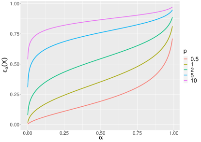
Figure 3: Graph of the $\alpha$-expectile function for $p\in\{0.5,1,2,5,10\}$.

Entropy

Entropy is a vital and widely studied subject in many fields. Entropy is a measure of the uncertainty related to a certain random variable. There are several types of entropy in the literature. The most commonly applied ones are Shannon’s, Rényi’s, and Tsallis’ entropy. We shall use the fact that the Matsuoka’s distribution is a member of the exponential family in the canonical form to derive a generalization of the entropies above, called the Sharma-Mittal entropy (see Nielsen and Nock,, 2011, and references therein). The Sharma-Mittal entropy of a random variable $X$ with a density $f_{\theta}$ is given by

$$H_{\alpha,\beta}(f_{\theta})\coloneqq\frac{1}{1-\beta}\bigg{[}\bigg{(}\int_{\mathds{R}}f_{\theta}(x)^{\alpha}dx\bigg{)}^{\frac{1-\beta}{1-\alpha}}-1\bigg{]},$$ (7)

Nielsen and Nock, (2011) shows that if $f_{\theta}$ is a member of the exponential family in canonical form, then

$$\mathcal{M}_{\alpha}(f_{\theta})\coloneqq\int_{\mathds{R}}f_{\theta}(x)^{\alpha}dx=\exp\Big{\{}\big{[}a(\alpha\theta)-\alpha a(\theta)\big{]}\mathds{E}\big{(}h(X)^{\alpha-1}\big{)}\Big{\}}.$$ (8)

If $X\sim\mathrm{M}(p)$, (8) becomes

$$\mathcal{M}_{\alpha}(f_{p}) =\int_{\mathds{R}}f_{p}(x)^{\alpha}dx=\alpha^{-\frac{3}{2}}p^{\frac{3(1-\alpha)}{2}}\bigg{[}\bigg{(}\frac{2}{\sqrt{\pi}}\bigg{)}^{\alpha}p^{\frac{3}{2}}\int_{0}^{1}\big{[}-\ln(x)\big{]}^{\alpha+\frac{1}{2}-1}x^{p-1}dx\bigg{]}$$

$$=\frac{\alpha^{-\frac{3}{2}}p^{3-\frac{\alpha}{2}}\Gamma\big{(}\alpha+\frac{3}{2}\big{)}}{(p-\alpha+1)^{\alpha+\frac{3}{2}}},$$ (9)

where the last integral is computed using the results in section 2 of Stacy, (1962). Substituting (2) in (7), we obtain the Sharma-Mittal entropy of $X\sim\mathrm{M}(p)$. Particular cases are Shannon’s entropy, $H_{S}(f_{p})\coloneqq-\mathds{E}(\ln(X))=\frac{3}{2p}$ obtained when both $\alpha,\beta\rightarrow 1$ (direct calculation is easier, though), Rényi’s entropy, $H_{R}(f_{p})\coloneqq\frac{1}{1-\alpha}\ln\bigl{(}\mathcal{M}_{\alpha}(f_{p})\big{)}$, obtained when $\beta\rightarrow 1$ and Tsalli’s entropy $H_{T}(f_{p})\coloneqq\frac{1}{1-\alpha}\big{(}\mathcal{M}_{\alpha}(f_{p})-1\big{)}$, obtained when $\beta\rightarrow\alpha$.

Stress-Strength Reliability

In reliability theory, stress-strength is a measure of the relationship between the strength of a unit and the stress imposed upon it. It is commonly defined as $R\coloneqq P(X>Y)$, and measures the probability that a unit $X$ is strong enough to withstand a random stress $Y$. This measure is useful and widely applied in many contexts, particularly in engineering. Let $X\sim\mathrm{M}(p)$ and $Y\sim\mathrm{M}(q)$ be independent random variables. The stress-strength reliability is given by

$$R =P(X>Y)=\int_{\mathds{R}}F_{q}(y)dF_{p}(y)=\frac{4p^{\frac{3}{2}}}{\pi}\int_{0}^{1}\sqrt{-\ln(y)}y^{q-1}\Gamma\bigg{(}\frac{3}{2},-q\ln(y)\bigg{)}dy$$

$$=\frac{4}{\pi}\bigg{(}\frac{p}{q}\bigg{)}^{\frac{3}{2}}\int_{0}^{\infty}u^{\frac{1}{2}}e^{-\frac{p}{q}u}\Gamma\bigg{(}\frac{3}{2},u\bigg{)}du,$$

where the last equality follows by changing variables to $u=-q\ln(y)$. Now, using equation 9.3.7 in volume II of Erdélyi et al., (1954) (p.138), setting $s\coloneqq\frac{p}{p+q}$, we obtain after some algebra,

$$R =\frac{4}{\pi}\bigg{(}\frac{p}{q}\bigg{)}^{\frac{3}{2}}\bigg{[}\frac{\Gamma(3)}{\frac{3}{2}(1+\frac{p}{q})^{3}}F\bigg{(}1,3;\frac{5}{2};s\bigg{)}\bigg{]}=\frac{16}{3\pi}[s(1-s)]^{\frac{3}{2}}F\bigg{(}1,3;\frac{5}{2};s\bigg{)},$$

where $F(a,b;c;x)$ is the hypergeometric function (see chapter 2 of Erdélyi et al.,, 1954, Volume I). Using elementary properties of the hypergeometric function (see section 2.8 of Erdélyi et al.,, 1954, Volume I), we can write

$$F\bigg{(}1,3;\frac{5}{2};s\bigg{)}=\frac{3}{8}\bigg{[}\frac{(1-2s)}{s(s-1)}+\frac{\arcsin\big{(}\sqrt{s}\big{)}}{[s(1-s)]^{\frac{3}{2}}}\bigg{]}.$$

Finally, after some simplifications we obtain

$$R=\frac{2}{\pi}\big{[}(2s-1)\sqrt{s(1-s)}+\arcsin\big{(}\sqrt{s}\big{)}\big{]}.$$

Figure 4 shows the behavior of the stress-strength probability $R$ for different values of $p$ and $q$.

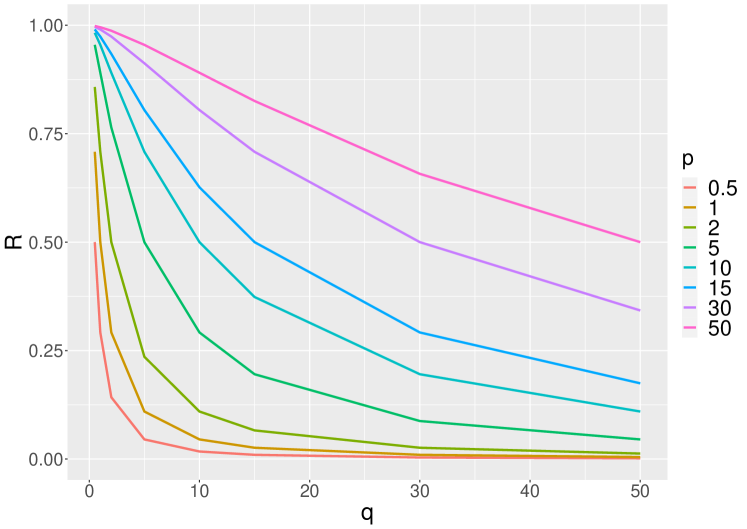
(a) $R$ curves for $p\in\{0.5,1,2,5,10,15,30,50\}$

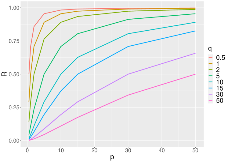
(b) $R$ curves for $q\in\{0.5,1,2,5,10,15,30,50\}$

Figure 4: Stress-strength reliability curves $R$ as functions of (a) $p$. and (b) $q$.

Order Statistics

Let $X_{1},\cdots,X_{n}$ be a random sample from the M($p$) distribution. Let $X_{(r)}$ denote the $r$th order statistic. Following Casella and Berger, (2002), and using that relation 8.356.3 in Gradshteyn and Ryzhik, (2007) ,we obtain

$$F_{X_{(r)}}(x)=\bigg{[}\frac{2}{\sqrt{\pi}}\bigg{]}^{n}\sum_{j=r}^{n}\binom{n}{j}\Gamma\bigg{(}\frac{3}{2},-p\ln(x)\bigg{)}^{j}\gamma\bigg{(}\frac{3}{2},-p\ln(x)\bigg{)}^{n-j}I(0<x<1)+I(x\geq 1).$$

The corresponding probability density function is given by

$$f_{X_{(r)}}(x)=r\binom{n}{r}\bigg{[}\frac{2}{\sqrt{\pi}}\bigg{]}^{n+1}x^{p-1}\sqrt{-p^{3}\ln(x)}\Gamma\bigg{(}\frac{3}{2},-p\ln(x)\biggr{)}^{r-1}\gamma\bigg{(}\frac{3}{2},-p\ln(x)\biggr{)}^{n-r},$$

for $0<x<1$, and $f_{X_{(r)}}(x)=0$ elsewhere. Figure 5 showcases the density of $X_{(1)}$, for fixed $p=2$ as the sample size $n$ increases.

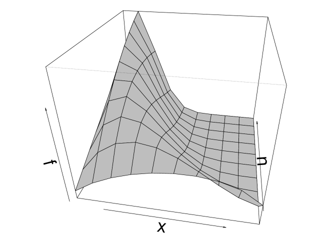
(a) $n=10$

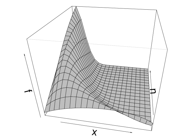
(b) $n=20$

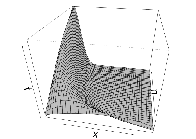
(c) $n=40$

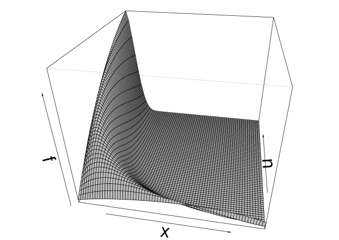
(d) $n=70$

Figure 5: Probability density function of $X_{(1)}$ for $p=2$ and $n\in\{10,20,40,70\}$.

3 Estimation of production frontiers

In economic theory, a production function is defined as the maximum output obtainable from a set of inputs, given a technology available to the firms involved. Formally, let $\boldsymbol{x}\in\mathds{R}_{+}^{m}$ be some inputs used to produce output $y\in\mathds{R}_{+}$, and denote the production set by $\Psi=\{(y,\boldsymbol{x})\in\mathds{R}_{+}^{m+1}:\boldsymbol{x}\text{ can produce }y\}$, where $\mathds{R}_{+}=\{z\in\mathds{R}:z\geq 0\}$. For all $\boldsymbol{x}\in\mathds{R}_{+}^{m}$, the production function, also known as the production frontier, associated with $\Psi$ is defined as $f(\boldsymbol{x})=\sup\{y\geq 0:(y,\boldsymbol{x})\in\Psi\}$. Moreover, for all pair $(y,\boldsymbol{x})\in\Psi$, let the efficiency be measured by the ratio $y/f(\boldsymbol{x})$.

From a statistical viewpoint, suppose that a random sample of production units $(Y_{i},\boldsymbol{X}_{i})_{i=1}^{n}$ taking values in $\Psi$ is observed and follows the model

$$Y_{i}=f(\boldsymbol{X}_{i})R_{i},\quad i\in\{1,\cdots,n\},$$ (10)

where $R_{i}\sim M(p)$ and $f:\mathds{R}^{m}\to\mathds{R}$ is a function that is multiplicative on unknown nonnegative smooth components $f_{j}$, i.e.,

$$f(\boldsymbol{X}_{i})=\prod_{j=1}^{m}f_{j}(X_{i,j}),$$

where $X_{i,j}$ denotes the $j$th component of $\boldsymbol{X}_{i}$. In this context, $R_{i}$ is the efficiency, $\boldsymbol{X}_{i}$ is the input vector, $Y_{i}$ is the output and $f$ is the production frontier. On one hand, values of $R_{i}$ close to $1$ are associated with values of $Y_{i}$ close to the frontier $f(\boldsymbol{X}_{i})$ and, consequently, are related to highly efficient firms. On the other hand, $Y_{i}$ being far from $f(\boldsymbol{X}_{i})$ implies low efficiency and small values of $R_{i}$. For simplicity, we assume that $R_{i}$ is independent of $\boldsymbol{X}_{i}$ and that $P(\boldsymbol{X}_{i}\in B_{i})=1$, for some $B_{i}\coloneqq\prod_{j=1}^{m}[a_{j},b_{j}]\subset\mathds{R}^{m}$.

Model (10) is motivated by the well-known Cobb-Douglas production function with $f$ taking the form $f(\boldsymbol{X}_{i})=a_{0}\prod_{j=1}^{m}X_{i,j}^{a_{j}},\ i\in\{1,\cdots,n\}$, where $a_{0},\cdots,a_{m}$ are parameters that quantify the responsiveness of the production function to changes in its respective arguments. This framework is appealing when one is considering interactions among input variables. A key property of such a function is that it is additive in log scale. The additivity alleviates the “curse of dimensionality” that arises in the multivariate nonparametric estimation (see Stone,, 1985).

Taking the logarithm on both sides of equation (10) allows us to rewrite the model as

$$Z_{i}=g(\boldsymbol{X}_{i})+\epsilon_{i},\quad i\in\{1,\cdots,n\},$$ (11)

where $Z_{i}\coloneqq-\ln(Y_{i})$ is the log-transformed data, $\epsilon_{i}\coloneqq-\ln(R_{i})-3/(2p)$ is a zero mean error term with variance $\sigma^{2}_{\epsilon}\coloneqq 3/(2p^{2})$ and the regression function becomes

$$g(\boldsymbol{X}_{i})=c_{0}+\sum_{j=1}^{m}g_{j}(X_{i,j})$$ (12)

with $c_{0}\coloneqq 3/(2p)$ and $g_{j}(X_{i,j})\coloneqq-\ln(f_{j}(X_{i,j}))$, $j\in\{1,\cdots,m\}$. As will be seem in the next subsection, for $m>1$, it will be required that $\mathds{E}(g_{j}(X_{i,j}))=0,\ j\in\{1,\cdots,m\}$. Hence, for the multivariate case, we will rewrite (12) by defining centered versions of the terms $c_{0}$ and $g_{j}$’s. We aim to estimate the parameter $p$ and the function $f$ which are assumed unknown in model (10). For this, we propose a three-step estimation procedure as detailed in the next subsections.

3.1 Step 1: estimation of the regression function $g$

Consider the $n$-vector of functions $g_{j}(\boldsymbol{x}_{j})\coloneqq(g_{j}(x_{1,j}),\cdots,g_{j}(x_{n,j}))^{\intercal}$ evaluated at grid points $\boldsymbol{x}_{j}=(x_{1,j},\cdots,x_{n,j})^{\intercal}$, $j\in\{1,\cdots,m\}$, and let $\boldsymbol{Z}\coloneqq(Z_{1},\cdots,Z_{n})^{\intercal}$ with $Z_{i}$ being given by equation (11) for all $i\in\{1,\cdots,n\}$.

We estimate each vector $g_{j}(\boldsymbol{x}_{j})$ using a linear smoother of the form

$$\hat{g}_{j}(\boldsymbol{x}_{j})\coloneqq W_{j}\boldsymbol{Z}^{\ast},\quad j\in\{1,\cdots,m\},$$ (13)

where $W_{j}$ is an $n\times n$ smoothing matrix, $Z^{\ast}\coloneqq\boldsymbol{Z}-\boldsymbol{\bar{Z}}$, with $\boldsymbol{\bar{Z}}\coloneqq\bar{Z}I(m>1)\boldsymbol{1}_{n}$, for $\boldsymbol{1}_{n}\coloneqq(1,\cdots,1)^{\intercal}\in\mathds{R}^{n}$ and $\bar{Z}=\frac{1}{n}\sum_{i=1}^{n}Z_{i}$. Note that when $m>1$ we are implicitly estimating the intercept $c_{0}$ using the sample mean. From (13), an estimator for the regression function $g$ is

$$\hat{g}(x_{i,1},\cdots,x_{i,m})=\boldsymbol{e}_{i,n}^{\intercal}\sum_{j=1}^{m}\hat{g}_{j}(\boldsymbol{x}_{j})+\bar{Z}I(m>1),\quad\forall i\in\{1,\cdots,n\},$$

where $\boldsymbol{e}_{i,n}$ is the $n$-vector with $1$ in the $i$th coordinate and $0$ everywhere else.

In this study, we restrict our attention to the local linear smoother (see Wand and Jones,, 1994; Tsybakov,, 2008, for a comprehensive overview of local polynomial regression), for the univariate inputs framework and the classical backfitting scheme, hereinafter referred to as CBS (Buja et al.,, 1989; Hastie and Tibshirani,, 1990) for bivariate inputs.

Before we proceed with the definition of the proposed estimator, let us introduce some notation. Let $K$ be a kernel function and, for bandwidths $h_{1},\cdots,h_{m}$, let $K_{h_{j}}(u)\coloneqq K(u/h_{j})/h_{j}$. For $z\in\mathds{R}$, let

$$A_{z}^{j}\coloneqq\left[\begin{array}[]{cc}1&(X_{1,j}-z)\\ \vdots&\vdots\\ 1&(X_{n,j}-z)\end{array}\right],$$

$D_{z}\coloneqq\operatorname*{diag}(K_{h_{j}}(X_{1,j}-z),\cdots,K_{h_{j}}(X_{n,j}-z))$, and let $\boldsymbol{w}_{j,z}$ be the equivalent kernel for $j$th covariate at the point $z$ defined by $\boldsymbol{w}_{j,z}^{\intercal}\coloneqq\boldsymbol{e}_{1,2}^{\intercal}({A_{z}^{j}}^{\intercal}D_{z}A_{z}^{j})^{-1}{A_{z}^{j}}^{\intercal}D_{z}$, provided that $({A_{z}^{j}}^{\intercal}D_{z}A_{z}^{j})^{-1}$ exists. Finally, let

$$S_{j}=(\boldsymbol{w}_{j,x_{1,j}},\cdots,\boldsymbol{w}_{j,x_{n,j}})^{\intercal},\quad j\in\{1,\cdots,m\}$$ (14)

Univariate case

For $m=1$, we estimate the regression function $g(\cdot)=c_{0}-\ln(f(\cdot))$ through the local linear estimator implying that the smoothing matrix is given by $W_{1}=S_{1}$ as defined in equation (14) for $j=1$. Thus, we estimate $g$ at point $x_{i,1}$ by

$$\hat{g}(x_{i,1})=\boldsymbol{e}_{i,n}^{\intercal}S_{1}\boldsymbol{Z},\quad i\in\{1,\cdots,n\}.$$ (15)

Bivariate case

For $m=2$, the regression function $g(x_{i,1},x_{i,2})=c_{0}+g_{1}(x_{i,1})+g_{2}(x_{i,2})$ is estimated using the CBS with local linear smoothers. For identification and estimation, it is required that the regression model (11)–(12) is such that $E(Z_{i})=c_{0}$ and $\mathds{E}(g_{j}(X_{i,j}))=0$, for all $j\in\{1,\cdots,m\}$ and $i\in\{1,\cdots,n\}$. Therefore, we need to rewrite equation (12) with $c_{0}=\frac{3}{2p}-\mathds{E}\big{(}\sum_{j=1}^{m}\ln\big{(}f_{j}(X_{i,j})\big{)}\big{)}$ and $g_{j}(X_{i,j})=\mathds{E}\big{(}\ln\big{(}f_{j}(X_{i,j})\big{)}\big{)}-\ln\big{(}f_{j}(X_{i,j})\big{)}$, $j\in\{1,\cdots,m\}$. As shown in Opsomer, (2000) and Hastie and Tibshirani, (1990), the related smoothing matrices admit explicit expressions and are given by

$$W_{1} =I_{n}-(I_{n}-S_{1}^{\ast}S_{2}^{\ast})^{-1}(I_{n}-S_{1}^{\ast});$$

$$W_{2} =I_{n}-(I_{n}-S_{2}^{\ast}S_{1}^{\ast})^{-1}(I_{n}-S_{2}^{\ast}),$$

provided that the inverses exist, where $S_{j}^{\ast}\coloneqq S_{j}-\big{(}\frac{1}{n}\sum_{i=1}^{n}S_{j}\big{)}\boldsymbol{1}_{n}$, with $S_{j}$ being defined analogously as in (14). As explained by Opsomer, (2000), the backfitting estimators for $g_{j}$’s at the observation points are obtained nonparametrically by solving a system of normal equations. Corollary 4.3 of Buja et al., (1989) proved that $\|S_{1}^{\ast}S_{2}^{\ast}\|<1$ is a sufficient condition for the existence of unique backfitting estimators when $m=2$, for any matrix norm $\|\cdot\|$. Therefore, we can estimate the regression function $g$ at $(x_{i,1},x_{i,2})$ by

$$\hat{g}(x_{i,1},x_{i,2})=\bar{Z}+\boldsymbol{e}_{i,n}^{\intercal}(W_{1}+W_{2})\boldsymbol{Z}^{\ast},\quad i\in\{1,\cdots,n\}.$$

3.2 Step 2: estimation of the parameter $p$

When the regression function $g$ in (11) is known, we have that $Z_{i}-g(\boldsymbol{X}_{i})=\epsilon_{i}$. We can then construct an estimator using the method of moments by equating the second sample moment with $\mathds{E}(\epsilon_{i}^{2})=3/(2p^{2})$ for which solution is given by the formula

$$\tilde{p}=\sqrt{\frac{3n}{2\sum_{i=1}^{n}\epsilon_{i}^{2}}}.$$

Clearly, $\tilde{p}$ is not feasible since $\{\epsilon_{i}\}_{i=1}^{n}$ is unobserved. We can approximate each $\epsilon_{i}=Z_{i}-g(\boldsymbol{X}_{i})$ by replacing $g$ with the first-step estimate $\hat{g}$, which in turn results in $\hat{\epsilon}_{i}=Z_{i}-\hat{g}(\boldsymbol{X}_{i}),\ i\in\{1,\cdots,n\}$. Therefore, a feasible estimator for $p$ is defined by

$$\hat{p}=\sqrt{\frac{3n}{2\sum_{i=1}^{n}\hat{\epsilon}_{i}^{2}}}.$$ (16)

3.3 Step 3: estimation of the production frontier $f$

By definition, $g(x)=-\ln(f(x))+3/(2p)$, which is equivalent to

$$f(x)=\exp\bigg{\{}\frac{3}{2p}-g(x)\bigg{\}}.$$ (17)

Thus, a straightforward feasible estimator for $f$ is obtained by replacing $p$ and $g(\cdot)$ with $\hat{p}$ and $\hat{g}(\cdot)$ respectively in (17), that is,

$$\hat{f}(x)=\exp\bigg{\{}\frac{3}{2\hat{p}}-\hat{g}(x)\bigg{\}}.$$ (18)

3.4 Asymptotic theory

In this section, we shall derive the asymptotic properties of the estimators presented in Sections 3.1–3.3. We will focus mainly on the univariate case for which most of the results required for our theory are available. Throughout this section, we denote by $C$ a generic positive constant which may take different values at different appearances.

Consider the case of univariate inputs, $X\in\mathds{R}_{+}$, and denote the density of $X$ by $f_{X}$. We make the following assumptions:

• Assumption 1. There exists $s>2$ such that $\mathds{E}(\lvert Z\rvert^{s})<C$ and $\displaystyle{\sup_{x\geq 0}}\Big{\{}\mathds{E}(\lvert Z\rvert^{s}|X=x)f_{X}(x)\big{\}}\leq C$. Moreover, it holds that $\displaystyle{\sup_{x\geq 0}}\big{\{}f_{X}(x)\big{\}}\leq C$.

• Assumption 2. The bandwidth satisfies $h=o(1)$ and $\ln(n)/(nh)=o(1)$, as $n\to\infty$.

• Assumption 3. The kernel $K:\mathds{R}\to\mathds{R}$ is symmetric, satisfies $\lvert u^{i}K(u)\rvert\leq C$ for $i\in\{0,1,2\}$, and $\int_{\mathds{R}}\lvert u^{j}K(u)\rvert du\leq C$ for $j\in\{0,1,2,4\}$. In addition, for some $\kappa<\infty$ and $L<\infty$, either $K(u)=0$ for all $u>L$ and for all $u,u^{\prime}\in\mathds{R}$

  $$\lvert K(u)-K(u^{\prime})\rvert\leq\kappa\lvert u-u^{\prime}\rvert,$$

  or $K(u)$ is differentiable, $\lvert\partial K(u)/\partial u\rvert\leq\kappa$, and $\lvert\partial K(u)/\partial u\rvert\leq\kappa\lvert u\rvert^{-v}$, for all $\lvert u\rvert>L$ and some $v>1$.

• Assumption 4. The second derivatives of $f_{X}(x)$ and $f_{X}(x)g(x)$ are uniformly continuous and bounded.

Assumption 1 specifies that the design density $f_{X}$ is bounded, gives uniform moment bounds for $Z$, and controls the tail behavior of the conditional expectation $\mathds{E}(\lvert Z\rvert^{s}|X=x)$, which is allowed to increase to infinity, but not faster than $f(x)^{-1}$. Assumption 2 is a strengthening of the usual condition that $h\to 0$ and $nh\to\infty$ as $n\to\infty$. Assumption 3 requires that function $K$ is bounded, integrable, and is either Lipschitz with compact support or has a bounded derivative with an integrable tail. Therefore, most of the commonly used kernels are allowed, including the Epanechnikov kernel (or more generally, polynomial kernels of the form $c(p)(1-x^{2})^{p}$), the Gaussian kernel, and some higher order kernels (e.g., those in Muller, (1984) and Wand and Schucany, (1990)).

The following theorem gives the rate of uniform convergence in probability and establishes the asymptotic normality for the estimator $\hat{g}$ presented in (15) (Section 3.1). Mathematical proofs are deferred to Appendix A.

Theorem 3.1.

Suppose that Assumptions 1-4 hold and that $\displaystyle{\min_{x\in[a,b]}}\big{\{}f_{X}(x)\big{\}}>0$ where $[a,b]=\mathrm{supp}(f_{X})$. Then

$$\max_{x\in[a,b]}\big{\{}\big{\lvert}\hat{g}(x)-g(x)\big{\rvert}\big{\}}=O_{p}\bigg{(}h^{2}+\sqrt{\frac{\ln(n)}{nh}}\bigg{)}.$$ (19)

If in addition the second derivative $g^{\prime\prime}(\cdot)$ is a continuous function and $nh^{3}\to\infty$, then for all point $x$ in the interior of $\mathrm{supp}(f_{X})$ for which the function $h(y)\coloneqq\mathds{E}(Z^{4}|X=y)$ is bounded on a neighborhood of $x$, we have that

$$\sqrt{nh}\big{[}\hat{g}(x)-g(x)-B(x)\big{]}\overset{d}{\longrightarrow}N(0,V(x)),$$ (20)

where

$$B(x)\coloneqq\frac{g^{\prime\prime}(x)h^{2}}{2}\int_{\mathds{R}}u^{2}K(u)du\quad\mbox{ and }\quad V(x)\coloneqq\frac{\sigma^{2}_{\epsilon}}{f_{X}(x)}\int_{\mathds{R}}K(u)^{2}du.$$

Methods for approximating the asymptotic conditional bias and variance in (20) are discussed in Sections 4.4 and 4.5 of Fan and Gijbels, (1996). The bias term $h^{2}$ in (19) can be eliminated if a second-order kernel is employed. As a result, the convergence achieves the optimal rate obtained by Stone, (1982). The next theorem gives the rate of uniform convergence in probability for estimators $\hat{p}$ and $\hat{f}$ introduced in (16) of Section 3.2 and in (18) of Section 3.3, respectively.

Theorem 3.2.

Suppose that Assumptions 1-4 hold and that $\displaystyle{\min_{x\in[a,b]}}\big{\{}f_{X}(x)\big{\}}>0$ where $[a,b]=\mathrm{supp}(f_{X})$. Then

$$\hat{p}-p=O_{p}\bigg{(}h^{2}+\sqrt{\frac{\ln(n)}{nh}}\bigg{)},$$

and

$$\max_{x\in[a,b]}\big{\{}\big{\lvert}\hat{f}(x)-f(x)\big{\rvert}\big{\}}=O_{p}\bigg{(}h^{2}+\sqrt{\frac{\ln(n)}{nh}}\bigg{)}.$$

The results in Theorems 3.1 and 3.2 indicate that the first step of the proposed estimation procedure is critical in the sense that the rate of the subsequent estimators is asymptotically dominated by that of the first one. The uniform convergence in Theorems 3.1 and 3.2 are established on an interval $[a,b]$, for simplicity. But one can consider a design density $f_{X}$ with unbounded support with the uniformity established on sets which slowly expands with $n$ at the cost of a penalty term in the rate of convergence in the same spirit as Hansen, (2008) (see theorem 10).

For the multivariate model, Opsomer and Ruppert, (1997) and Opsomer, (2000) derived sufficient conditions for the existence and uniqueness of the backfitting estimator with local polynomial smoother. For these estimators, they also provided a formula for the associated conditional bias and variance. The extension of our results to the bivariate case is non-trivial and depends on results that are still ongoing research themes.

4 Simulations

In this section, we investigate the finite sample behavior of the estimators presented in Sections 3.1 – 3.3 via Monte Carlo experiments. We simulate model (10) through the following data-generating process (DGP) with either univariate or bivariate inputs:

• Random samples are generated from $Y_{i}=f(X_{i})R_{i}$, for all $i\in\{1,\cdots,n\}$, with $f(X_{i})=-X_{i}^{2}+4X_{i}$, and $X_{i}\sim U(1,2)$ being independent of $R_{i}\sim M(p)$;

• Random samples are generated from $Y_{i}=f(X_{i})R_{i}$, for all $i\in\{1,\cdots,n\}$, with $f(X_{i})=\exp(-f_{1}(X_{i,1})-f_{2}(X_{i,2}))$, $f_{1}(x)=-1.5x^{2}+3x-1$, $f_{2}(x)=-(\ln(x)+1)/2+\ln(2)$, and $X_{i,1}\sim U(1,2)$, $X_{i,2}\sim U(1,2)$ and $R_{i}\sim M(p)$ being mutually independent.

These experiments are repeated $N=1{,}000$ times for each combination of sample size $n\in\{100,150,250\}$ and parameter $p\in\{1,2,8\}$.

The performance of the estimators $\hat{f}$ and $\hat{g}$ is assessed by the mean averaged squared error (MASE). Let $\hat{m}$ be an estimator of $m$, and suppose $N$ replicas are available. For a realization $(x_{1,r},\cdots,x_{n,r})$ from $\boldsymbol{X}$, $\mathrm{ASE}_{r}(\hat{m})\coloneqq n^{-1}\sum_{i=1}^{n}(\hat{m}(x_{i,r})-m(x_{i,r}))^{2}$ is computed for each $r\in\{1,\cdots,N\}$. Then, MASE is defined as $L(\hat{m})\coloneqq N^{-1}\sum_{r=1}^{N}ASE_{r}(\hat{m})$. We carried out the estimation with the Epanechnikov kernel and the leave-one-out bandwidth defined by equation (23) in Appendix B. The simulation was performed using the software R version 4.2.3 (R Core Team,, 2023). The code was implemented by the authors and are available on github.com/marciovalk/Frontier-Estimation—Matsuoka-distribution. The incomplete and inverse incomplete gamma function were calculated using the zipfR library (Evert and Baroni,, 2007).

DGP (i): univariate inputs

Simulation results for univariate inputs are summarized in Table 1, which reports MASE values for estimators $\hat{f}$ and $\hat{g}$, and expected values, variances, and quantiles 0.05 and 0.95 for $\hat{p}$. Observe that, the MASE and $\mathrm{Var}(\hat{p})$ values decrease to zero, as $n$ increases, while the expected value of $\hat{p}$ approximates $p$, which is evidence that the estimates uniformly approach their respective true values.

Table 1: Monte Carlo simulation results for univariate inputs.

$p$	$n$	$L(\hat{f})$	$L(\hat{g})$	$\mathds{E}(\hat{p})$	$\mathrm{Var}(\hat{p})$	$Q_{.05}(\hat{p})$	$Q_{.95}(\hat{p})$
1	$100$	0.63	0.04	1.04	0.02	0.85	1.25
	$150$	0.42	0.03	1.03	0.01	0.86	1.19
	$250$	0.26	0.02	1.02	0.01	0.89	1.15
2	$100$	0.16	0.01	2.07	0.06	1.69	2.48
	$150$	0.11	0.01	2.06	0.04	1.74	2.40
	$250$	0.07	0.00	2.03	0.03	1.78	2.30
8	$100$	0.01	0.00	8.30	1.06	6.72	10.10
	$150$	0.01	0.00	8.24	0.66	6.96	9.59
	$250$	0.01	0.00	8.15	0.40	7.17	9.21

Table 1 suggests that the MASE values for $\hat{g}$ and $\hat{f}$ are larger for smaller values of $p$. Figure 6 provides a visual presentation of $n=100$ simulated data points from DGP (i) for $p\in\{1,8\}$. from the plots, it is clear that the variance of the error term is bigger when $p=1$. For instance, $\sigma^{2}_{\epsilon}\simeq 1.5$ for $p=1$, whereas $\sigma^{2}_{\epsilon}\simeq 0.02$ for $p=8$. This behavior is expected since, from Theorem 3.1 of Fan and Gijbels, (1996), the conditional variance of $\hat{g}$ is given by $\mathrm{Var}(\hat{g}(x)|\boldsymbol{X})=\sigma^{2}_{\epsilon}v_{0}[f_{X}(x)nh]^{-1}+o_{p}(1/(nh))$, where $v_{0}=\int K^{2}(u)du$ and $f_{X}$ is the design density of $\boldsymbol{X}$. On the other hand, the conditional bias is $\mathrm{Bias}(\hat{g}(x)|\boldsymbol{X})=\frac{1}{2}h^{2}g^{\prime\prime}(x)\mu_{2}+o_{p}(h^{2})$ where $g^{\prime\prime}$ is the second derivative of $g$ and $\mu_{2}=\int u^{2}K(u)du$. Thus, when parameter $p$ varies, the leading term of $\mathrm{Var}(\hat{g}(x)|\boldsymbol{X})$ is affected by $\sigma_{\epsilon}^{2}$. Hence, small values of $p$ imply a large error variance as $\sigma^{2}_{\epsilon}=\frac{3}{2p^{2}}$, which in turn results in an increased variance for the local linear estimator $\hat{g}$.

Under mild conditions, it can be shown (lemma 4.2 in Xia and Li,, 2002) that the averaged square error $\mathrm{ASE}(\hat{g})\coloneqq n^{-1}\sum_{i=1}^{n}(\hat{g}(X_{i})-g(X_{i}))^{2}$ is asymptotically equivalent to the mean integrated squared error (MISE) defined by $\int\mathds{E}[(g(x)-\hat{g}(x))^{2}]f_{X}(x)dx=\int[\mathrm{Bias}(\hat{g}(x))^{2}+\mathrm{Var}(\hat{g}(x))]f_{X}(x)dx$ from where the positive relationship between $L(\hat{g})$ and $\mathrm{Var}(\hat{g})$ can be traced back to. If smaller values of $p$ tend to increase $\mathrm{ASE}(\hat{g})$ via $\mathrm{Var}(\hat{g})$, then they also tend to increase $\mathds{E}\big{(}\mathrm{ASE}(\hat{g})\big{)}$, which is approximated by $L(\hat{g})$. Moreover, the third step estimator $\hat{f}$ seems to be dominated by the estimation errors of $\hat{g}$: $L(\hat{f})$ is large (small) if $L(\hat{g})$ was large (small).

Figure 6: Simulated data for $p=1$ and $p=8$.

Table 1 indicates that the bias and the variance of $\hat{p}$ depend positively on $p$. Moreover, we infer that $\hat{p}$ inherits the fact that the unfeasible estimator $\tilde{p}$ overestimates $p$ which can be seen through repeated applications of Jensen’s inequality as follows

$$\mathds{E}(\tilde{p})>\sqrt{\frac{3n}{2}}\frac{1}{\mathds{E}\Big{(}\sqrt{\sum_{i=1}^{n}\epsilon_{i}^{2}}\Big{)}}\geq\sqrt{\frac{3n}{2}}\frac{1}{\sqrt{\sum_{i=1}^{n}E(\epsilon_{i}^{2})}}=p.$$

Figure 7 presents boxplots and histograms of the simulation results for different values of $p\in\{1,2,8\}$ and $n\in\{100,150,250\}$. The plots show finite sample evidence of the consistency of $\hat{p}$ obtained in Theorem 3.2, but also of its asymptotic normality, although some bias is present.On the other hand, in Figure 8 we observe that $\mathrm{ASE}_{r}(\hat{f})$ and $\mathrm{ASE}_{r}(\hat{g})$ decrease to values close to zero as the sample size increases, but still showing some bias. Aside from the scale, we observe that the behavior of $\mathrm{ASE}_{r}(\hat{f})$ and $\mathrm{ASE}_{r}(\hat{g})$ are quite similar.

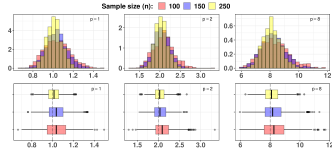
Figure 7: Boxplots of the estimated values $\hat{p}$ for the univariate case.

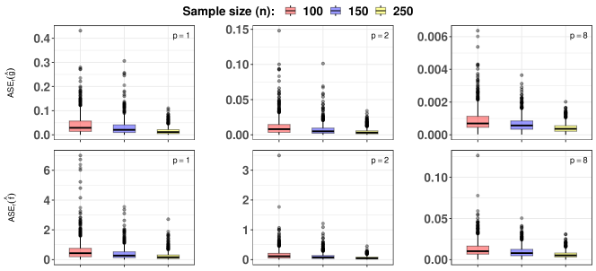
Figure 8: Boxplots of the values $\mathrm{ASE}_{r}(\hat{g})$ and $\mathrm{ASE}_{r}(\hat{f})$ for the univariate case.

DGP (ii): bivariate inputs

Table 2: Monte Carlo simulation results for the case of bivariate inputs.

$p$	$n$	$L(\hat{f})$	$L(\hat{g})$	$L(\hat{g}_{1})$	$L(\hat{g}_{2})$	$\mathds{E}(\hat{p})$	$\mathrm{Var}(\hat{p})$	$Q_{.05}(\hat{p})$	$Q_{.95}(\hat{p})$
1	$100$	0.17	0.09	0.04	0.04	1.07	0.02	0.87	1.29
	$150$	0.10	0.06	0.03	0.02	1.04	0.01	0.88	1.23
	$250$	0.07	0.04	0.02	0.01	1.03	0.01	0.90	1.17
2	$100$	0.05	0.03	0.01	0.01	2.13	0.07	1.75	2.58
	$150$	0.03	0.02	0.01	0.01	2.09	0.04	1.80	2.44
	$250$	0.02	0.01	0.01	0.00	2.05	0.02	1.80	2.31
8	$100$	0.00	0.00	0.00	0.00	8.56	1.26	6.82	10.47
	$150$	0.00	0.00	0.00	0.00	8.37	0.68	7.09	9.80
	$250$	0.00	0.00	0.00	0.00	8.24	0.42	7.21	9.30

Simulation results for the case of bivariate inputs are summarized in Table 2. In general, the conclusions are quite similar to those in the univariate approach: (a) they indicate that the estimates get closer to their respective true values as the sample size increases; (b) the MASE values for $\hat{g}$, $\hat{g}_{1}$, $\hat{g}_{2}$, and $\hat{f}$ are larger for smaller values of $p$; and (c) $\hat{p}$ tend to overestimate $p$ and its bias and variance depend positively on the value of $p$. Figure 9 present boxplots (top row) and histograms (bottom row) of the estimated values considering $p\in\{1,2,8\}$ and $n\in\{100,150,250\}$, whereas Figure 10 presents boxplots of the estimated values of $\mathrm{ASE}_{r}(\hat{f})$ (top row) and $\mathrm{ASE}_{r}(\hat{g})$ (bottom row) as a function of $p$ and $n$, for $r\in\{1,\cdots,N\}$. The boxplots in Figure 9 clearly depicts the estimation bias of $\hat{p}$ which causes the histograms to be slightly positively asymmetric, especially for small values of $n$. The $\mathrm{ASE}_{r}(\hat{f})$ and $\mathrm{ASE}_{r}(\hat{g})$ shown in Figure 10 are very similar in behavior to the univariate case, decreasing to values close to zero as the sample size increases, but still showing some bias.

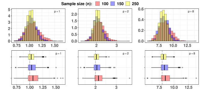
Figure 9: Boxplots of the estimated values $\hat{p}$ for the bivariate case.

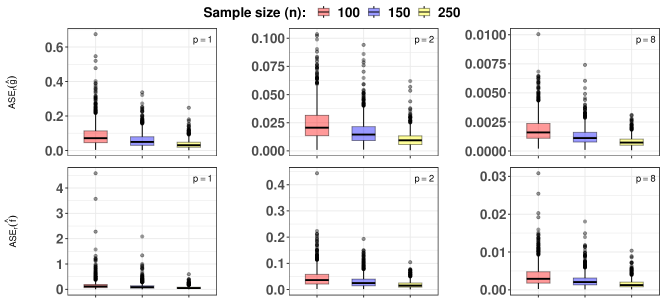
Figure 10: Boxplots of the values $\mathrm{ASE}_{r}(\hat{g})$ and $\mathrm{ASE}_{r}(\hat{f})$ for the bivariate case.

5 Empirical application

In what follows, we apply our three-step estimation procedure to the Danish Milk producers data set available in the R package Benchmarking (for more details, see Bogetoft and Otto,, 2022). The data set consists of $n=108$ observations, where output of milk per cow is taken as the response variable, whereas veterinary expenses per cow ($X_{1}$) and energy expenses per cow ($X_{2}$) are used as covariates. We apply model (10) to estimate the production frontier $f$. The estimation is carried out using the Gaussian kernel, with bandwidth selected using the leave-one-out method outlined in Appendix B.

Figure 11: Estimates of component functions $g_{1}(X_{1})$ and $g_{2}(X_{2})$.

Figure 11 depicts the estimated component functions $\hat{g}_{1}(x_{1})$ and $\hat{g}_{2}(x_{2})$. By hypothesis, recall that each component function is given by $g_{j}(X_{j})=-\ln\big{(}f_{j}(X_{j})\big{)}+c$, where $c\coloneqq\mathds{E}\big{(}\ln(f_{j}(X_{j}))\big{)}$ is a scalar. Let $x$ be a point in the domain of $g_{j}$ and denote the first and the second derivatives of a function $\ell$ by $\ell^{\prime}$ and $\ell^{\prime\prime}$ respectively. Firstly, note that $g_{j}^{\prime}(x)=-f_{j}^{\prime}(x)/f_{j}(x)$. If $g^{\prime}(x)\leq 0$, then $f^{\prime}_{j}(x)\geq 0$ since $f_{j}(x)\geq 0$ by hypothesis. Therefore, the estimates of $g_{1}$ and $g_{2}$ in Figure 11, which are downward sloped, indicate that components $f_{1}$ and $f_{2}$ are increasing functions. In other words, milk production increases with veterinary and energy expenses. In addition, we have that $g_{j}^{\prime\prime}(x)=(f_{j}^{\prime}(x)/f_{j}(x))^{2}-f_{j}^{\prime\prime}(x)/f_{j}(x)$. Thus, if $g_{j}^{\prime\prime}(x)\leq 0$, then $f_{j}^{\prime}(x)^{2}\leq f_{j}^{\prime\prime}(x)f_{j}(x)$ which in turn implies that $f_{j}^{\prime\prime}(x)\geq 0$, since $f_{j}$ is a nonnegative function. On the right side of Figure 11, we can see that $\hat{g}_{2}$ has a concave shape on a substantial portion of its domain (roughly from $0.2$ to $1$). This suggests the presence of increasing marginal returns for energy expenses.

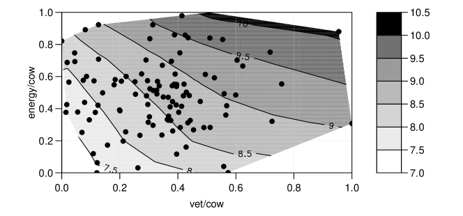
Figure 12: Contour lines of the estimated production function $\hat{f}$.

Figure 12 shows the isoquants obtained from the estimated production frontier $\hat{f}(x_{1},x_{2})$ on the convex hull determined by the data points. In general, the isoquants are downward sloping, indicating that the production function $f$ increases with partial increments in veterinary and energy expenses. Especially for lower values of milk production, the isoquants are convex, suggesting that $f$ is quasi-concave on the associated set of inputs. The shape change of isoquants, which look flatter for higher values of milk, indicates changes in the veterinary productivity relative to energy, which in economic terms means that the patterns of the marginal rates of technical substitution are changing along the output levels – see Chapter 9 of Nicholson and Snyder, (2007). This suggests that the relative productivity of veterinary expenses is lower for higher levels of milk. The estimated value of $p$ is $\hat{p}\simeq 8.53$ which suggests that the probability distribution of the efficiency is highly left-skewed.

6 Conclusion and discussion

In this work we introduced a univariate uniparametric distribution in $(0,1)$, called Matsuoka’s distribution, and derived some of its basic properties, such as quantiles, moments, and some related measures, the Sharma-Mittal entropy, the stress-strength reliability, $\alpha$-expectiles, among others. Due to its simplicity and flexibility, we introduced a production frontier model where the efficiency variable was assumed to follow Matsuoka’s distribution. This allowed the proposal and study of a semiparametric three-step estimation procedure for estimating the unknown production frontier and the unknown parameter related to efficiency. Asymptotic results were obtained under standard assumptions. In the asymptotic analysis, we argued that the first step of our estimation procedure is important, in the sense that its estimation error dominates the rate of convergence of all subsequent steps.

Monte Carlo simulation results showcased the finite sample properties of the proposed methodology, which resemble the theoretical ones obtained. Moreover, our results suggest that the proposed method of moments estimator for $\hat{p}$ tends to overestimate $p$, with bias and variance positively related with $p$.

Finally, the proposed methodology is applied to investigate the dynamics of the Danish milk production data, focusing in production frontier estimation. The output of milk per cow is taken as the response variable, while veterinary and energy expenses per cow are used as covariates. In general, our analysis reveals that the milk production increases in response to partial increments on veterinary and energy expenses. Notably, we found the presence of increasing marginal returns for energy expenses, pointing to the possibility that higher levels of energy investment result in proportionally greater gains in milk production. Furthermore, our examination of the marginal rates of technical substitution reveals dynamic patterns across varying output levels, implying a nuanced interplay between input factors. Particularly noteworthy is the observed decrease in the relative productivity of veterinary expenses at higher levels of milk production, suggesting a complex relationship between inputs and milk production.

Appendix A. Proofs

Proof of Theorem 3.1: The proof follows by direct applications of Theorem 10 of Hansen, (2008) for the uniform rate of convergence in (19) and Theorem 5.2 of Fan and Gijbels, (1996) for the asymptotic normality in (20), and thus is omitted.

Proof of Theorem 3.2: We start with the estimator $\hat{p}$. Write $\hat{p}-p=(\hat{p}-\tilde{p})+(\tilde{p}-p)\coloneqq A_{1,n}+A_{2,n}$. Given $\varepsilon>0$, from Theorem 3.1 and Minkowski’s inequality for differences, writing $a_{n}\coloneqq h^{2}+\sqrt{\ln(n)/(nh)}$, it follows that

$$P\bigg{(} \frac{1}{a_{n}\sqrt{n}}\bigg{|}\bigg{(}\sum_{i=1}^{n}\hat{\epsilon}_{i}^{2}\biggr{)}^{\frac{1}{2}}-\bigg{(}\sum_{i=1}^{n}\epsilon_{i}^{2}\biggr{)}^{\frac{1}{2}}\bigg{|}>\varepsilon\bigg{)}\leq P\bigg{(}\frac{1}{a_{n}\sqrt{n}}\bigg{[}\sum_{i=1}^{n}(\hat{\epsilon}_{i}-\epsilon_{i})^{2}\bigg{]}^{\frac{1}{2}}>\varepsilon\bigg{)}=$$

$$=P\bigg{(}\frac{1}{a_{n}^{2}n}\sum_{i=1}^{n}(\hat{\epsilon}_{i}-\epsilon_{i})^{2}>\varepsilon^{2}\bigg{)}\leq P\bigg{(}\frac{1}{a_{n}^{2}}\max_{1\leq i\leq n}\big{\{}(\hat{\epsilon}_{i}-\epsilon_{i})^{2}\big{\}}>\varepsilon^{2}\bigg{)}\leq$$

$$\leq P\bigg{(}\frac{1}{a_{n}^{2}}\max_{1\leq i\leq n}\big{\{}\big{(}\hat{g}(X_{i})-g(X_{i})\big{)}^{2}\big{\}}>\varepsilon^{2}\bigg{)}\leq P\bigg{(}\frac{1}{a_{n}}\max_{a\leq x\leq b}\big{\{}\big{|}\hat{g}(x)-g(x)\big{|}\big{\}}>\varepsilon\bigg{)}=o(1).$$

As a consequence,

$$\sqrt{\frac{2}{3}}\hat{p}=\bigg{(}\frac{1}{n}\sum_{i=1}^{n}\hat{\epsilon}_{i}^{2}\biggr{)}^{-\frac{1}{2}}=\bigg{(}\frac{1}{n}\sum_{i=1}^{n}\epsilon_{i}^{2}+O_{p}(a_{n})\biggr{)}^{-\frac{1}{2}}=\bigg{(}\frac{1}{n}\sum_{i=1}^{n}\epsilon_{i}^{2}\biggr{)}^{-\frac{1}{2}}+O_{p}(a_{n}),$$ (21)

since $a_{n}\rightarrow 0$. Multiplying both sides of equation (21) by $\sqrt{3/2}$ yields $\hat{p}=\tilde{p}+O_{p}(a_{n})$, or equivalently, $A_{1,n}=O_{p}(a_{n})$.

Now we show that the term $A_{2,n}$ is asymptotically dominated by $A_{1,n}$. For brevity, denote $\xi_{i}\coloneqq\epsilon_{i}^{2}$. Then $\mathds{E}(\xi_{i})=\frac{3}{2p^{2}}$ and $\sigma^{2}_{\xi}\coloneqq\mathrm{Var}(\xi_{i})=\frac{27}{2p^{4}}$. By the Central Limit Theorem, it follows that

$$\frac{1}{\sqrt{n}}\sum_{i=1}^{n}[\xi_{i}-\mathds{E}(\xi_{i})]\overset{d}{\longrightarrow}N(0,\sigma^{2}_{\xi}).$$

Considering the function $\ell_{1}(u)\coloneqq\sqrt{\frac{3}{2u}}$, whose first derivative is $\ell_{1}^{\prime}(u)=-\sqrt{\frac{3}{8u^{3}}}$, the Delta method yields

$$\sqrt{n}(\tilde{p}-p)=\frac{1}{\sqrt{n}}\sum_{i=1}^{n}[\ell_{1}(\xi_{i})-\ell_{1}(\mathds{E}(\xi_{i}))]\overset{d}{\longrightarrow}N(0,\sigma^{2}_{\xi}[\ell_{1}^{\prime}(\sigma^{2}_{\xi})]^{2}).$$

Since $\sqrt{n}(\tilde{p}-p)$ converges to a Gaussian limit, it is bounded in probability (theorem 2.4(i) of Van der Vaart,, 1998), i.e., $A_{2,n}=O_{p}(n^{-\frac{1}{2}})=o_{p}(a_{n})$, since $a_{n}\sqrt{n}\to\infty$. We conclude that $\hat{p}-p=a_{n}[O_{p}(1)+o_{p}(1)]=O_{p}(a_{n})$ as desired.

Next, consider the estimator $\hat{f}$. Theorem 3.1 and the result obtained above for $\hat{p}$ imply respectively that $\displaystyle{\max_{x\in[a,b]}}\big{\{}\big{|}\hat{g}(x)-g(x)\big{|}\big{\}}=o_{p}(1)$ and $|\hat{p}-p|=o_{p}(1)$, since $a_{n}=o(1)$ by hypothesis. Furthermore, for all $c>0$,

$$P\bigg{(}\max_{x\in[a,b]}\Big{\{}\big{|} \ln\big{(}\hat{f}(x)/a_{n}\big{)}-\ln\big{(}f(x)/a_{n}\big{)}\big{|}\Big{\}}>c\bigg{)}=$$

$$=P\bigg{(}\max_{x\in[a,b]}\Big{\{}\Big{|}\ln(\hat{f}(x))-\ln\big{(}e^{\frac{3}{2p}-g(x)}\big{)}\Big{|}\Big{\}}>c\bigg{)}$$

$$=P\bigg{(}\max_{x\in[a,b]}\bigg{\{}\bigg{|}\frac{3}{2\hat{p}}-\frac{3}{2p}-\hat{g}(x)+g(x)\bigg{|}\bigg{\}}>c\bigg{)}$$

$$\leq P\bigg{(}\bigg{\lvert}\frac{3}{2\hat{p}}-\frac{3}{2p}\bigg{\rvert}>\frac{c}{2}\bigg{)}+P\bigg{(}\max_{x\in[a,b]}\Big{\{}\Big{|}\hat{g}(x)-g(x)\Big{|}\Big{\}}>\frac{c}{2}\bigg{)}\coloneqq B_{1,n}+B_{2,n}.$$

It is clear that $B_{2,n}=o(1)$. Now since $\ell_{2}(u)\coloneqq 3/(2u)$ is a continuous function on $(0,\infty)$ and $\hat{p}>0$ almost surely, then the continuous mapping theorem (Theorem 2.3(ii) of Van der Vaart,, 1998) implies that $B_{1,n}=o(1)$ as well. Let $l_{3}(u)\coloneqq e^{u}$. For all $x\in[a,b]$ and $c>0$, the continuity of $l_{3}(\cdot)$ implies that there is $c_{2}>0$ such that

$$P\Big{(}\big{\lvert}\hat{f}(x)-f(x)\big{\rvert}>ca_{n}\Big{)} =P\bigg{(}\big{\lvert}\ell_{3}\big{(}\ln\big{(}\hat{f}(x)/a_{n}\big{)}\big{)}-\ell_{3}\big{(}\ln\big{(}f(x)/a_{n}\big{)}\big{)}\big{\rvert}>c\bigg{)}$$

$$\leq P\bigg{(}\big{\lvert}\ln\big{(}\hat{f}(x)/a_{n}\big{)}-\ln\big{(}f(x)/a_{n}\big{)}\big{\rvert}>c_{2}\bigg{)}+o(1)=o(1),$$ (22)

where the last equality holds because we have shown above that $\ln(\hat{f}(x)/a_{n})-\ln(f(x)/a_{n})=o_{p}(1)$ uniformly on $x\in[a,b]$. Since (Appendix A. Proofs) holds for all $x\in[a,b]$, it also holds for

$$x_{0}\coloneqq\underset{x\in[a,b]}{\operatorname*{arg\,max}}\big{\{}\big{|}\hat{f}(x)-f(x)\big{|}\big{\}},$$

and the proof is complete.  

Appendix B. Cross-validation bandwidth selection

The nonparametric estimator employed in the first step of our estimation procedure requires the choice of a bandwidth (also called smoothing parameter). The bandwidth selection is usually done by a cross-validation algorithm or a plug-in method (see Wand and Jones,, 1994; Fan and Gijbels,, 1996).

In this study, we focus on the leave-one-out technique which is a cross-validation method and relies on minimizing the following loss function on a set $H\subseteq\mathds{R}^{m}$ conditionally to $\boldsymbol{X}=(\boldsymbol{X}_{1},\cdots,\boldsymbol{X}_{n})$:

$$CV(\boldsymbol{h}|\boldsymbol{X})=\frac{1}{n}\sum_{i=1}^{n}(Z_{i}-\hat{g}_{-i}(\boldsymbol{X}_{i}))^{2},$$

where $\hat{g}_{-i}$ is the estimate of $g$ calculated from the subsample $\{(Y_{j},\boldsymbol{X}_{j})\}_{j\neq i}^{n}$ for all $i\in\{1,\cdots,n\}$ with $\boldsymbol{X}_{j}\in\mathds{R}^{m}$. We define the leave-one-out bandwidth as

$$\boldsymbol{h}_{cv}=\operatorname*{arg\,min}_{\boldsymbol{h}\in H}\{CV(\boldsymbol{h}|\boldsymbol{X})\}.$$ (23)

References

• Bezat, (2009) Bezat, A. (2009). Comparison of the deterministic and stochastic approaches for estimating technical efficiency on the example of non-parametric DEA and parametric SFA methods. Metody Ilościowe w Badaniach Ekonomicznych, 10(1):20–29.
• Bickel and Doksum, (2007) Bickel, P. J. and Doksum, K. A. (2007). Mathematical statistics: basic ideas and selected topics, volume I. CRC Press, 2nd edition.
• Bogetoft and Otto, (2010) Bogetoft, P. and Otto, L. (2010). Benchmarking with DEA, SFA, and R, volume 157. Springer Science & Business Media.
• Bogetoft and Otto, (2022) Bogetoft, P. and Otto, L. (2022). Benchmarking with DEA and SFA. R package version 0.31.
• Buja et al., (1989) Buja, A., Hastie, T., and Tibshirani, R. (1989). Linear smoothers and additive models. The Annals of Statistics, pages 453–510.
• Cascos and Ochoa, (2021) Cascos, I. and Ochoa, M. (2021). Expectile depth: Theory and computation for bivariate datasets. Journal of Multivariate Analysis, 184:104757.
• Casella and Berger, (2002) Casella, G. and Berger, R. (2002). Statistical Inference. Duxbury Resource Center.
• Charnes et al., (1978) Charnes, A., Cooper, W. W., and Rhodes, E. (1978). Measuring the efficiency of decision making units. European Journal of Operational Research, 2(6):429–444.
• Consul and Jain, (1971) Consul, P. C. and Jain, G. C. (1971). On the log-gamma distribution and its properties. Statistische Hefte, 12:100–106.
• Deprins et al., (2006) Deprins, D., Simar, L., and Tulkens, H. (2006). Measuring Labor-Efficiency in Post Offices, pages 285–309. Springer US, Boston, MA.
• Diebold and Rudebusch, (1990) Diebold, F. X. and Rudebusch, G. D. (1990). A nonparametric investigation of duration dependence in the American business cycle. Journal of Political Economy, 98(3):596–616.
• Eckstein and Wolpin, (1995) Eckstein, Z. and Wolpin, K. I. (1995). Duration to first job and the return to schooling: estimates from a search-matching model. The Review of Economic Studies, 62(2):263–286.
• Erdélyi et al., (1954) Erdélyi et al., A. (1954). Higher Transcendental Functions, vols. I, II, and III. McGraw Hill, New York.
• Evert and Baroni, (2007) Evert, S. and Baroni, M. (2007). zipfR: Word frequency distributions in R. In Proceedings of the 45th Annual Meeting of the Association for Computational Linguistics, Posters and Demonstrations Sessions, pages 29–32, Prague, Czech Republic. (R package version 0.6-70 of 2020-10-10).
• Fan and Gijbels, (1996) Fan, J. and Gijbels, I. (1996). Local polynomial modelling and its applications: monographs on statistics and applied probability 66, volume 66. CRC Press.
• Farrell, (1957) Farrell, M. J. (1957). The measurement of productive efficiency. Journal of the Royal Statistical Society. Series A (General), 120(3):253–290.
• Favero et al., (1994) Favero, C. A., Pesaran, M. H., and Sharma, S. (1994). A duration model of irreversible oil investment: theory and empirical evidence. Journal of Applied Econometrics, 9(S1):S95–S112.
• Gradshteyn and Ryzhik, (2007) Gradshteyn, I. S. and Ryzhik, I. M. (2007). Table of integrals, series, and products. Academic Press, 7 edition.
• Halliwell, (2021) Halliwell, L. J. (2021). The Log-Gamma distribution and non-normal error. Variance, 13.
• Hansen, (2008) Hansen, B. E. (2008). Uniform convergence rates for kernel estimation with dependent data. Econometric Theory, 24(3):726–748.
• Hastie and Tibshirani, (1990) Hastie, T. J. and Tibshirani, J. S. (1990). Generalized additive models. Chapman and Hall.
• Hogg and Klugman, (1984) Hogg, R. V. and Klugman, S. A. (1984). Loss distributions. John Wiley & Sons.
• Lancaster, (1979) Lancaster, T. (1979). Econometric methods for the duration of unemployment. Econometrica: Journal of the Econometric Society, pages 939–956.
• Muller, (1984) Muller, H.-G. (1984). Smooth optimum kernel estimators of densities, regression curves and modes. The Annals of Statistics, pages 766–774.
• Nicholson and Snyder, (2007) Nicholson, W. and Snyder, C. M. (2007). Microeconomic theory: Basic principles and extensions. Thomson South-Western, 10th edition.
• Nielsen and Nock, (2011) Nielsen, F. and Nock, R. (2011). A closed-form expression for the Sharma-Mittal entropy of exponential families. Journal of Physics A: Mathematical and Theoretical, 45(3):032003.
• Opsomer, (2000) Opsomer, J. D. (2000). Asymptotic properties of backfitting estimators. Journal of Multivariate Analysis, 73(2):166–179.
• Opsomer and Ruppert, (1997) Opsomer, J. D. and Ruppert, D. (1997). Fitting a bivariate additive model by local polynomial regression. The Annals of Statistics, 25(1):186–211.
• R Core Team, (2023) R Core Team (2023). R: A Language and Environment for Statistical Computing. R Foundation for Statistical Computing, Vienna, Austria.
• Schnabel and Eilers, (2009) Schnabel, S. K. and Eilers, P. H. (2009). Optimal expectile smoothing. Computational Statistics & Data Analysis, 53(12):4168–4177.
• Stacy, (1962) Stacy, E. W. (1962). A generalization of the gamma distribution. The Annals of mathematical statistics, pages 1187–1192.
• Stahlschmidt et al., (2014) Stahlschmidt, S., Eckardt, M., and Härdle, W. K. (2014). Expectile treatment effects: An efficient alternative to compute the distribution of treatment effects. SFB 649 Discussion Paper 2014-059, Humboldt University of Berlin, Berlin.
• Stone, (1982) Stone, C. J. (1982). Optimal global rates of convergence for nonparametric regression. The annals of statistics, pages 1040–1053.
• Stone, (1985) Stone, C. J. (1985). Additive regression and other nonparametric models. The annals of Statistics, 13(2):689–705.
• Tsybakov, (2008) Tsybakov, A. (2008). Introduction to Nonparametric Estimation. Springer Series in Statistics. Springer New York.
• Tzavidis et al., (2010) Tzavidis, N., Salvati, N., Geraci, M., and Bottai, M. (2010). M-quantile and expectile random effects regression for multilevel data. Working paper, Southampton Statistical Sciences Research Institute.
• Van der Vaart, (1998) Van der Vaart, A. W. (1998). Asymptotic statistics. Cambridge University Press.
• Wand and Jones, (1994) Wand, M. P. and Jones, M. C. (1994). Kernel smoothing. Chapman and Hall/CRC.
• Wand and Schucany, (1990) Wand, M. P. and Schucany, W. R. (1990). Gaussian-based kernels. Canadian Journal of Statistics, 18(3):197–204.
• Xia and Li, (2002) Xia, Y. and Li, W. K. (2002). Asymptotic behavior of bandwidth selected by the cross-validation method for local polynomial fitting. Journal of multivariate analysis, 83(2):265–287.