The Impact of Symmetry Handling for the
Stable Set Problem via Schreier-Sims Cuts

Abstract

Symmetry handling inequalities (SHIs) are an appealing and popular tool for handling symmetries in integer programming. Despite their practical application, little is known about their interaction with optimization problems. This article focuses on Schreier-Sims (SST) cuts, a recently introduced family of SHIs, and investigate their impact on the computational and polyhedral complexity of optimization problems. Given that SST cuts are not unique, a crucial question is to understand how different constructions of SST cuts influence the solving process.

First, we observe that SST cuts do not increase the computational complexity of solving a linear optimization problem over any polytope $P$. However, separating the integer hull of $P$ enriched by SST cuts can be NP-hard, even if $P$ is integral and has a compact formulation. We study this phenomenon more in-depth for the stable set problem, particularly for subclasses of perfect graphs. For bipartite graphs, we give a complete characterization of the integer hull after adding SST cuts based on odd-cycle inequalities. For trivially perfect graphs, we observe that the separation problem is still NP-hard after adding a generic set of SST cuts. Our main contribution is to identify a specific class of SST cuts, called stringent SST cuts, that keeps the separation problem polynomial and a complete set of inequalities, namely SST clique cuts, that yield a complete linear description.

We complement these results by giving SST cuts based presolving techniques and provide a computational study to compare the different approaches. In particular, our newly identified stringent SST cuts dominate other approaches.

Keywords: symmetry handling, stable set, perfect graph, totally unimodular

1 Introduction

Handling symmetries in integer programs has the goal to speed up the solution process by avoiding the consideration of symmetric solutions. Although many techniques have been developed for this goal, only little is known about the interaction of symmetry handling methods and structures of the problem to be solved. In this article we try to shed light on this interplay for a classical problem in integer programming and combinatorial optimization: the stable set problem.

In the stable set problem, we are given an undirected simple graph $G=(V,E)$ and a (nonnegative) weight $c_{v}$ for each node $v\in V$. The goal is to find a set of nodes $S\subseteq V$ of maximal weight $\sum_{v\in S}c_{v}$ that is stable, i.e., no two nodes of $S$ are connected by an edge. One common integer programming formulation for this problem is:

$$\max_{x\in\{0,1\}^{V}}\,\Big{\{}\sum_{v\in V}c_{v}\,x_{v}\;:\;x_{u}+x_{v}\leq 1\quad\forall\,\{u,v\}\in E\Big{\}}.$$

Assume that the set of nodes is $V=\{1,\dots,n\}$. As is often the case, we consider permutation symmetries, i.e., subgroups of the symmetric group $\mathcal{S}_{n}$ of all permutations of $[n]\coloneqq\{1,\dots,n\}$. A permutation $\gamma$ acts on $x\in\mathds{R}^{n}$ by permuting its coordinates, i.e., $\gamma(x)\coloneqq(x_{{\gamma}^{-1}(1)},\dots,x_{{\gamma}^{-1}(n)})$. A subgroup $\Gamma\leq\mathcal{S}_{n}$ is a symmetry group of the above integer program if every $\gamma\in\Gamma$ maps feasible solutions onto feasible solutions while preserving their objective values. If all weights are equal to 1, i.e., we consider the maximum stable set problem, a symmetry group $\Gamma$ is given by the automorphisms of the graph !$G$, i.e., permutations $\gamma\colon V\to V$, where $\{\gamma(u),\gamma(v)\}\in E$ if and only if $\{u,v\}\in E$. These symmetries can be computed efficiently in practice by graph automorphism software like nauty/traces [36, 35], saucy [7, 6], and bliss [22, 23, 21].

One line of research for handling symmetries is based on so-called symmetry handling inequalities (SHIs), which cut a subset of symmetric solutions off, while keeping at least one (optimal) solution intact. An intuitive class of SHIs can be derived from the Schreier-Sims Table (SST), which has been proposed by Liberti and Ostrowski [31] and Salvagnin [43]. These so-called SST cuts are of the form $x_{j}\leq x_{i}$ for some carefully selected set of pairs of variable indices $i$ and $j$. They can be constructed in polynomial time if we are given a set of generators of $\Gamma$, see Section 2 for details. Note that the set of SST cuts is not unique, since the variables that yield SST cuts can be selected in different ways. Moreover, regardless of the choice of SST cuts, they yield an inclusionwise minimal closed symmetry breaking set: any smaller closed subset $\mathcal{K}{}^{\prime}$ would leave some orbit $\mathrm{orb}(x,\Gamma)\coloneqq\{\gamma(x):\gamma\in\Gamma\}$ without an element in $\mathcal{K}{}^{\prime}$ [52].

The main topic of this paper is formulated in the following leading question:

What is the impact of adding SST cuts on the complexity of the stable set problem, both in theory and practice?

More specifically, we ask whether different types of SST cuts behave differently with respect to solving the stable set problem.

Clearly, one would hope that neither the computational nor polyhedral complexity increases when adding SST cuts. But the answer to the above question is not immediate in general, since SST cuts might change the structure of the underlying problem. In particular, an increase in complexity could occur for the stable set problem in graph classes admitting exact polynomial time algorithms. On the upside, the benefits of SST cuts come by a potential increase in solution speed when using enumerative techniques, for example, branch-and-cut.

Our Contribution.

First, we show that an optimal solution satisfying SST cuts can be computed in polynomial time, if the underlying problem is solvable in polynomial time. This is shown for general binary optimization problems, including the stable set case. When considering the integer hull of a polytope, however, the situation is different. We show that if the integer hull of a polytope can be efficiently separated, then the problem of separating the integer hull after adding SST cuts can be NP-hard. That is, the complexity of first computing the integer hull of a problem and then applying SST cuts differs from first adding SST cuts and then computing the integer hull. Moreover, this result holds even when the original polytope is defined by a totally unimodular matrix and an integral right hand side (hence yielding an integral polytope). In particular, we can lose integrality by adding the SST cuts, meaning that the linear programming relaxations become weaker, negatively affecting their solution time.

The previous general result suggests a rich interplay between SST cuts and the underlying polytope. To study this phenomenon in more detail, we focus on the stable set polytope $P(G)$ for a perfect graph $G$. Perfect graphs are a well-studied class of graphs where the maximum stable set problem is solvable in polynomial time [14]. Moreover, a complete description of $P(G)$ is given by considering box constraints and clique cuts, that is, a constraint for each maximal clique, that guarantees that at most one node in the clique is selected. For perfect graphs, clique cuts can be separated in polynomial time [14]. For a set of SST cuts $S$, let $P(G,S)$ denote the integer hull of $P(G)$ intersected with the SST cuts in $S$. For subclasses of perfect graphs, we consider the problem of finding a complete description of $P(G,S)$. We study two widely studied subclasses: bipartite graphs and trivially perfect graphs. Unsurprisingly, for both cases we can lose integrality if we add SST cuts to the clique formulation of $P(G)$.

For bipartite graphs, we present an explicit family of inequalities that describes $P(G,S)$ and can be separated in polynomial time. To show this result we provide an extended formulation of $P(G,S)$ based on an auxiliary graph $G^{\prime}$; this works for arbitrary graphs, not necessarily bipartite. We observe that in the case of bipartite graphs, graph $G^{\prime}$ is almost bipartite, that is, removing a single vertex yields a bipartite graph. We can exploit this structure and the fact that almost bipartite graphs are ($t$-)perfect to obtain our result. So, in particular, for this subclass of graphs, the complexity of separating $P(G,S)$ is still polynomial, regardless of the choice of SST cuts $S$.

A more subtle landscape is found when considering trivially perfect graphs. These are interval graphs whose collection of intervals forms a laminar family. In this case the clique formulation is totally unimodular [13]. Interestingly, we can show that even in this simple scenario the separation problem $P(G,S)$ remains NP-hard. Inquiring deeper, we notice that the reduction works for only a particular family of SST cuts, that is, for a specific choice of variables appearing in the cuts. Our main technical contribution is identifying a specific construction of SST cuts, called stringent SST cuts, and showing that they behave well for trivially perfect graphs, namely $P(G,S)$ can be separated in polynomial time, and even can be described with a quadratic number of inequalities. Moreover, an explicit linear description of $P(G,S)$ is given by considering so-called SST clique cuts, a strengthening of the SST cuts that incorporate information of the graph’s structure. To show our theorem, we derive an auxiliary graph that shrinks some cliques, yielding a reduced graph where SST clique cuts become regular SST cuts. For this simpler case, we show that extending the clique matrix with SST cuts yields a totally unimodular matrix. This is proved by giving a explicit interpretation of this matrix as a network matrix, which are known to be totally unimodular [45].

Additionally, we consider the effects of SST cuts on presolving. We show that one can delete certain nodes or add edges, which represent implications of SST cuts for optimal solutions. Finally, we study how our results impact computations. In particular we study the effect of presolving, adding SST cuts, adding SST clique cuts, and the choice of SST (clique) cuts, in particular of the stringency property. Over our testset, the best results are given by first performing SST presolving for stringent cuts, recomputing symmetries and then adding stringent SST clique cuts. This yields a speed-up of about $15\text{\,}\mathrm{\char 37\relax}$ on average for our testset of 82 instances with respect to the default settings.

Our results leave as an open problem whether $P(G,S)$ can be separated in polynomial time if $G$ is a perfect graph and $S$ are stringent.

Literature Review.

The literature mainly discusses two lines of research to handle symmetries in binary programs: the addition of (static) symmetry handling inequalities to the problem formulation, which restricts the search space of the original problem, and dynamic symmetry handling techniques, which modify the branch-and-bound algorithm based on symmetry information, see, among others, [33, 34, 38, 39, 40, 32]. In this article, we follow the former line of research.

A standard technique for deriving symmetry handling inequalities is to enforce that among a set of symmetric solutions only those should be computed that are lexicographically maximal. Here, we say that two solutions $x$ and $y$ of a binary program with symmetry group $\Gamma\leq\mathcal{S}_{n}$ are symmetric if there exists $\gamma\in\Gamma$ such that $y=\gamma(x)$. The set of all symmetric solutions of $x$ is called the orbit of $x$, denoted $\mathrm{orb}(x,\Gamma)\coloneqq\{\gamma(x)\,:\,\gamma\in\Gamma\}$. By overloading notation, we denote the orbits of variable indices $i\in[n]$ by $\mathrm{orb}(i,\Gamma)=\{\gamma(i)\,:\,\gamma\in\Gamma\}$. Moreover, we say that a vector $x$ is lexicographically smaller or equal to vector $y$, denoted $x\preceq_{\mathrm{lex}}y$, if either $x=y$ or $x_{i}<y_{i}$ for the first position $i$ in which $x$ and $y$ differ. If $\mathcal{X}$ is the feasible region of a binary program, a valid symmetry handling approach is to restrict the feasible region to $\mathcal{X}\cap\{x\in\{0,1\}^{n}\,:\,\gamma(x)\preceq_{\mathrm{lex}}x\text{ for all }\gamma\in\Gamma\}$.

Friedman [11] describes how the lexicographic restriction can be modeled by linear inequalities, which potentially need exponentially large coefficients. Since this might cause numerical instabilities, an alternative set of inequalities with $\{0,\pm 1\}$-coefficients is in [19]. The alternative set of inequalities for $\gamma(x)\preceq_{\mathrm{lex}}x$ is derived via a knapsack polytope associated with $\operatorname{conv}\{x\in\{0,1\}^{n}\,:\,\gamma(x)\preceq_{\mathrm{lex}}x\}$ for a fixed permutation $\gamma$, the so-called symresack. Although the alternative set of inequalities is exponentially large, they can be separated in almost linear time [19], which has been improved to linear time [2]. A linear time propagation algorithm for the constraint $\gamma(x)\preceq_{\mathrm{lex}}x$ also exists [51]. Moreover, there exists a family of permutations such that in each integer programming formulation of a symresack, the size of coefficients or the number of inequalities needs to be exponentially large [17].

A drawback of Friedman’s approach is that one needs to add a constraint for each permutation in a group. But for specific symmetry groups, stronger results can be achieved. If the symmetry group $\Gamma$ is cyclic, efficient propagation algorithms for $\{x\in\{0,1\}^{n}\,:\,\gamma(x)\preceq_{\mathrm{lex}}x\text{ for all }\gamma\in\Gamma\}$ are described in [51]. If the variables of a binary program can be arranged in a matrix $X\in\{0,1\}^{p\times q}$ with ${n=p\cdot q}$, and the symmetry group $\Gamma$ acts on the variables by permuting the columns of $X$, the lexicographic restriction boils down to sort the columns in lexicographic order, i.e., to enforce ${X^{i+1}\preceq_{\mathrm{lex}}X^{i}}$ for all $i\in[q-1]$, where $X^{i}$ denotes the $i$-th column of $X$. Bendotti et al. [1] describe a linear time propagation algorithm for the set $\mathcal{X}^{p,q}\coloneqq\{X\in\{0,1\}^{p\times q}\,:\,X^{i+1}\preceq_{\mathrm{lex}}X^{i}\text{ for all }i\in[q-1]\}$. Moreover, if additionally every row of $X$ has at most/exactly one 1-entry, a complete linear description of the convex hull of these matrices, the so-called packing/partitioning orbitope, is known [26] and can be propagated in linear time [25]. In general, however, a complete linear description of $\operatorname{conv}(\mathcal{X}^{p,q})$ is unknown [24] except for the case $q=2$ and $p=1$ [19]. That is, the strongest symmetry handling inequalities are unknown in general.

For general groups, Liberti [30] suggests to select a single variable $x_{i}$ and to add the inequalities $x_{i}\geq x_{j}$ for all $j\in\mathrm{orb}(i,\Gamma)$. These inequalities partially handle symmetries of a single orbit of $\Gamma$ and can only be used for a single variable. By considering a subgroup, this idea can be iterated for a different variable. We detail this approach in the next section as these inequalities form the main object of interest of this article.

2 Schreier-Sims Table Inequalities

Recall the symmetry handling inequalities $x_{i}\geq x_{j}$ for $j\in\mathrm{orb}(i,\Gamma)$ and a fixed $i\in[n]$. As described above, one drawback of these inequalities is that they only handle symmetries on a single variable orbit and thus they might be rather weak. A simple idea to strengthen this approach is to add these inequalities for multiple orbits. To be able to combine symmetry handling inequalities for different orbits, Liberti and Ostrowski [31] and Salvagnin [43] suggest to focus on subgroups for subsequent choices of variables. This modification requires the concepts of stabilizers and orbits of the symmetry group.

Let $\Gamma\leq\mathcal{S}_{n}$ be a symmetry group of the binary program. The pointwise stabilizer of a set $I\subseteq[n]$ is $\mathrm{stab}(\Gamma,I)\coloneqq\{\gamma\in\Gamma\,:\,\gamma(i)=i\text{ for }i\in I\}$. If $\Gamma$ is given by a set of generating permutations $\Pi\subseteq\Gamma$, generators of the stabilizer can be computed in time polynomial in $n$ and $\lvert{\Pi}\rvert$ via the so-called Schreier-Sims table, see, e.g., [46]. In particular, the number of generators of the stabilizer group is polynomial. Since variable orbits $\mathrm{orb}(i,\Gamma)$ can also be computed in time polynomial in $n$ and $\lvert{\Pi}\rvert$, see [46], also orbits of stabilizer groups can be computed in polynomial time.

Using these concepts, an extended family of symmetry handling inequalities can be found by the following so-called SST algorithm. It initializes $\Gamma^{\prime}\leftarrow\Gamma$ and a sequence $L\leftarrow\emptyset$. Afterwards, the following steps are repeated:

1. select $\ell\in[n]\setminus L$ and compute $O_{\ell}\leftarrow\mathrm{orb}(\ell,\Gamma^{\prime})$;

2. append $\ell$ to $L$ and update $\Gamma^{\prime}\leftarrow\mathrm{stab}(\Gamma^{\prime},L)$;

3. repeat the previous steps until $L=[n]$.

Due to the above discussion, this algorithm runs in polynomial time. Moreover, note that we can terminate the SST algorithm once the group $\Gamma^{\prime}$ becomes trivial. For technical reasons in Section 4.2.2, however, we do not include this check in the SST algorithm.

At termination, $L$ denotes an ordered sequence in $[n]$. Each element $\ell$ in $L$ is called a leader and each $f\in O_{\ell}\setminus\{\ell\}$ is a follower of $\ell$. In the following, we will also use set notation for $L$, e.g., $\ell\in L$ for some element $\ell$ in the sequence. For $\ell\in L$ and $f\in O_{\ell}\setminus\{\ell\}$, a Schreier-Sims Table (SST) cut is:

$$-x_{\ell}+x_{f}\leq 0,$$

which for binary variables says that the selection the follower $f$, i.e., $x_{f}=1$, implies $x_{\ell}=1$. Due to the modification of the group in each step of the algorithm, all SST cuts can be used simultaneously to handle symmetries. We refer the reader to [31, 43] for details on correctness.

We usually refer to a single SST cut by a pair $(\ell,f)$ with $\ell\in L$ and $f\in O_{\ell}\setminus\{\ell\}$. Moreover, $S(L)\coloneqq\{(\ell,f)\,:\,\ell\in L,\;f\in O_{\ell}\setminus\{\ell\}\}$ denotes the set of all SST cuts. A set $S\subseteq S(L)$ of SST cuts defines the cone

$$\mathcal{K}(S)\coloneqq\{x\in\mathds{R}^{n}\,:\,-x_{\ell}+x_{f}\leq 0\text{ for all }(\ell,f)\in S\}.$$

3 Complexity

In this section we study the effect that SST cuts have on the complexity of an optimization problem. First, we show that adding SST cuts to a polynomial time solvable binary optimization problem keeps the problem polynomial. We will assume that the symmetry group of the problem $\Gamma$ is given by a set of $\text{poly}(n)$ generators, which always exists [46]. We state the theorem for binary programs, but the result directly applies to a generalized problem $\max\,\{{c}^{\top}{x}\,:\,x\in\mathcal{X}\}$ as long as a generating set of the symmetry group $\Gamma\leq\mathcal{S}_{n}$ is given as input.

Theorem 3.1.

Assume that the program $\max\,\{{c}^{\top}{x}\,:\,Ax\leq b,\;x\in\{0,1\}^{n}\}$ has $\Gamma\leq\mathcal{S}_{n}$ as symmetry group and that it can be solved in $T$ time. For leaders $L$ derived from $\Gamma$ and SST cuts $S=S(L)$, we can solve optimally $\max\,\{{c}^{\top}{x}\,:\,Ax\leq b,\;x\in\{0,1\}^{n},\;x\in\mathcal{K}(S)\}$ in $T+\text{poly}(n)$ time.

Proof.

Let $\hat{x}$ be an optimal solution of $\max\,\{{c}^{\top}{x}\,:\,Ax\leq b,\;x\in\{0,1\}^{n}\}$. We construct an optimal solution $\hat{x}^{\prime}$ for $\max\,\{{c}^{\top}{x}\,:\,Ax\leq b,\;x\in\{0,1\}^{n},\;x\in\mathcal{K}(S)\}$ in polynomial time. Consider the first leader $\ell_{1}\in L$ and let $i_{1}\in\operatorname{argmax}\,\{\hat{x}_{i}\,:\,i\in O_{\ell_{1}}\}$ and $\gamma\in\Gamma$ be such that $\gamma(i_{1})=\ell_{1}$. Then, $\gamma(\hat{x})$ satisfies the SST cuts $-x_{\ell_{1}}+x_{f}\leq 0$ for all $f\in O_{\ell_{1}}$. By replacing $\Gamma$ by the stabilizer of $\ell_{1}$ and $\hat{x}$ by $\gamma(\hat{x})$, we can iterate the procedure for the remaining orbits to find a point $\hat{x}^{\prime}\in\mathrm{orb}(x,\Gamma)$ that satisfies all SST cuts. Since $\hat{x}$ is optimal, $\hat{x}^{\prime}$ is optimal too. Since pointwise stabilizers can be computed in polynomial time [46, Ch. 4], $\hat{x}^{\prime}$ can be constructed in polynomial time. ∎

Next we focus on the interaction of SST cuts and the integer hull of a polytope. For two given natural numbers $m$ and $\ell$, consider the following polytope

$$P_{m,\ell}\coloneqq\Big{\{}x\in\mathds{R}_{+}^{m\times\ell}:\sum_{i=1}^{m}x_{ij}\leq 1\text{ for all }j\in\{1,\ldots,\ell\}\Big{\}}.$$

A binary matrix $x\in P_{m,\ell}\cap\mathds{Z}^{m\times\ell}$ contains at most one 1-entry in each column. Moreover, $P_{m,\ell}$ is integral, which can be seen either by using total unimodularity or sparsity of the set of constraints. Consider $\Gamma=\mathcal{S}_{\ell}$, the symmetric group on $[\ell]$, acting on $x\in\mathds{R}^{m\times\ell}$ by permuting columns, that is, for $\gamma\in\Gamma$ we have that $\gamma(x)=(x_{i,\gamma^{-1}(j)})_{i,j}$. Then $\Gamma$ is a symmetry group of the polytope $P_{m,\ell}$. The next theorem attests that $\text{int.hull}(P_{m,\ell}\cap\mathcal{K}(S(L)))$ is NP-hard to separate, where $\text{int.hull}(P)=\operatorname{conv}(P\cap\mathds{Z}^{n})$ denotes the integer hull of $P\subseteq\mathds{R}^{n}$.

Theorem 3.2.

Consider the polytope $P_{m,\ell}\subseteq\mathds{R}^{m\times\ell}$ with symmetry group $\Gamma=\mathcal{S}_{\ell}$ acting on $\mathds{R}^{m\times\ell}$ by column permutations. There exists a sequence of leaders $L$ for $\Gamma$ such that $\text{int.hull}(P_{m,\ell}\cap\mathcal{K}(S(L)))$ is NP-hard to separate.

Proof.

Let $w\in\mathds{Q}^{m\times\ell}$ be some weight function. We will show that, for a specific choice of leaders $L$, the problem of finding $x\in\text{int.hull}(P_{m,\ell}\cap\mathcal{K}(L))$ that maximizes ${w}^{\top}{x}=\sum_{i=1}^{m}\sum_{j=1}^{\ell}w_{ij}x_{ij}$ is NP-hard. This is enough to show the lemma due to the equivalence of optimization and separation [15].

Let us consider the following instance of 3D-matching. Let $X$, $Y$, $Z$ be three pairwise disjoint sets with $k$ elements each. We are given a collection of sets $\mathcal{T}\subseteq 2^{X\cup Y\cup Z}$, where $T\in\mathcal{T}$ is of the form $\{T_{X},T_{Y},T_{Z}\}$ with $T_{X}\in X$, $T_{Y}\in Y$, and $T_{Z}\in Z$. We must decide whether a 3D-matching exists, that is, if there exists a collection $\mathcal{T}^{\prime}\subseteq\mathcal{T}$ that partitions $X\cup Y\cup Z$, i.e., for any $a\in X\cup Y\cup Z$ there exists exactly one $T\in\mathcal{T}^{\prime}$ such that $a\in T$. It is well known that this decision problem is NP-complete [27].

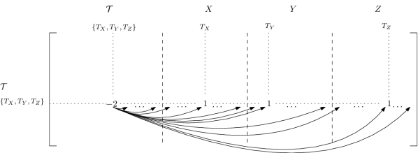
Figure 1: Scheme depicting the indices of a matrix $x\in P_{m,\ell}$ and weight matrix $w$. Rows are indexed by elements in $\mathcal{T}$ while columns by $\mathcal{T}\cup X\cup Y\cup Z$. The numbers displayed represent the coefficients of $w$ in the corresponding entry; entries not displayed on row $\{T_{X},T_{Y},T_{Z}\}$ are 0. Arrows represent SST cuts, where the tail is the leader and the head the follower.

To construct our polytope, we define $m=\lvert{\mathcal{T}}\rvert$ and $\ell=\lvert{\mathcal{T}}\rvert+3k$ and consider the polytope $P=P_{m,\ell}$. For a matrix $x\in P$ we can identify the indices of the rows with the set $\mathcal{T}$. Similarly, due to the definition of $\ell$ we can identify the indices of columns of $x\in P$ with $\mathcal{T}\cup X\cup Y\cup Z$; see Figure 1 for an schematic. Hence, a binary matrix $x$ belongs to $P_{m,\ell}$ if and only if at most one entry of the vector $(x_{T,b})_{T\in\mathcal{T}}$ is 1, for each $b\in\mathcal{T}\cup X\cup Y\cup Z$. As before, we define $\Gamma$ as the symmetric group $\mathcal{S}(\mathcal{T}\cup X\cup Y\cup Z)=\mathcal{S}_{\ell}$ that acts on $\mathds{R}^{m\times\ell}$ by permuting the columns.

We define a weight vector $w$ as

$$w_{T,b}=\begin{cases}-2&\text{ if }b=T,\\ 1&\text{ if }b\in T,\\ 0&\text{ otherwise},\end{cases}$$

for $T\in\mathcal{T}$ and $b\in\mathcal{T}\cup X\cup Y\cup Z$.

Let us consider an arbitrary order of the collection $\mathcal{T}$ given by $T_{1}$, $T_{2}$, …, $T_{m}$. We consider the SST cuts where the $i$th leader is $(T_{i},T_{i})$. Hence, for a given leader $(T_{i},T_{i})$ its corresponding SST cuts are

$$x_{T_{i},b}\leq x_{T_{i},T_{i}}\text{ where }b=T_{j}\text{ for some }j>i\text{, or }b\in X\cup Y\cup Z.$$ (1)

This set of inequalities defines the SST cut polyhedron $\mathcal{K}(S)$. The proof will be completed by showing the following result.

Claim.

There exists $x\in\text{int.hull}(P_{m,\ell}\cap\mathcal{K}(S))$ with ${w}^{\top}{x}\geq k$ if an only if the initial instance admits a 3D-matching.

To show the claim, let us first assume that $\mathcal{T}^{\prime}\subseteq\mathcal{T}$ is a 3D-matching. Consider the matrix $x$ defined as follows. For any row $T=\{T_{X},T_{Y},T_{Z}\}\in\mathcal{T}^{\prime}$ of the 3D-matching, we add four 1-entries, one per column indexed by $T$, $T_{X}$, $T_{Y}$ and $T_{Z}$. The rest of the entries are defined as zero. More precisely, we define

$$x_{T,b}=\begin{cases}1&\text{ if }T\in\mathcal{T}^{\prime}\text{ and }b=T,\\ 1&\text{ if }T\in\mathcal{T}^{\prime}\text{ and }b\in T,\\ 0&\text{ otherwise.}\end{cases}$$

First, observe that ${w}^{\top}{x}=k$, as any row of $x$ indexed by $T\in\mathcal{T}^{\prime}$ contributes exactly $-2+1+1+1=1$ to the total sum of ${w}^{\top}{x}=\lvert{\mathcal{T}^{\prime}}\rvert=k$. Clearly $x$ is integral. Let us now argue that $x\in P_{m,\ell}\cap\mathcal{K}(S)$. Indeed, for any column indexed by $T$, $x$ has exactly one 1-entry if $T\in\mathcal{T}^{\prime}$, and no 1-entries otherwise. Consider now a column indexed by $b\in X\cup Y\cup Z$. Then, by construction of $x$, the entries of $x$ that equal 1 within column $b$ are $x_{T,b}$ where $b\in T$ and $T\in\mathcal{T}^{\prime}$. As $\mathcal{T}^{\prime}$ is a 3D-matching, column $b$ must have exactly one 1-entry. We hence conclude that $x\in P_{m,\ell}$. Finally, we note that the SST cuts (1) are satisfied. Indeed, we either have that row $T$ of $x$ is identical to 0, if $T\not\in\mathcal{T}^{\prime}$, or $x_{T,T}=1$ if $T\in\mathcal{T}^{\prime}$. In either case the SST-cuts are satisfied by definition.

Conversely, let $x$ be a binary matrix in $P_{m,\ell}\cap\mathcal{K}(S)$ with ${w}^{\top}{x}\geq k$. Moreover, among all possible matrices $x$, choose one with a minimum number of 1-entries. Let us construct a 3D-matching. Indeed, we define the set $\mathcal{T}^{\prime}\subseteq\mathcal{T}$ of all $T$ such that $x_{T,T}=1$. The SST-cuts imply that any row $T\not\in\mathcal{T}^{\prime}$ does not contribute anything to the objective function, since $\sum_{b\in\mathcal{T}\cup X\cup Y\cup Z}w_{T,b}\,x_{T,b}=0$. Furthermore, each row of $w$ sums to $-2+1+1+1=1$, and hence, for each $T\in\mathcal{T}^{\prime}$ it holds that $\sum_{b\in\mathcal{T}\cup X\cup Y\cup Z}w_{T,b}\,x_{T,b}\leq 1$ since $x$ is binary and satisfies the SST cuts. Moreover, if $\sum_{b\in\mathcal{T}\cup X\cup Y\cup Z}w_{T,b}\,x_{T,b}\leq 0$, we could change the complete row $T$ to be zero. This would yield another vector $x\in\text{int.hull}(P_{m,\ell}\cap\mathcal{K}(S))$ with ${w}^{\top}{x}\geq k$, contradicting the minimality of $x$. Hence we conclude that $\sum_{b\in\mathcal{T}\cup X\cup Y\cup Z}w_{T,b}x_{T,b}=1$ for each $T\in\mathcal{T}^{\prime}$. In other words, for any $T\in\mathcal{T}$ and $b\in X\cup Y\cup Z$, we obtain that $x_{T,b}=1$ if and only if $T\in\mathcal{T}^{\prime}$ and $b\in T$. In particular, this implies that $\lvert{\mathcal{T}^{\prime}}\rvert={w}^{\top}{x}\geq k$.

Let us use this to show that $\mathcal{T}^{\prime}$ is a 3D-matching. Notice that if $T$, $T^{\prime}\in\mathcal{T}^{\prime}$, then $T$ and $T^{\prime}$ are disjoint. Indeed, if $b\in T\cap T^{\prime}$, then $x_{T,b}=x_{T^{\prime},b}=1$, which would violate the inequalities of $P_{m,\ell}$. Hence, $\mathcal{T}$ contains at least $k$ sets, which are pair-wise disjoint. This already implies that $\mathcal{T}^{\prime}$ is a 3D-matching, as $\lvert{\bigcup_{T\in\mathcal{T}^{\prime}}T}\rvert\geq 3k$, and hence $\mathcal{T}^{\prime}$ must cover all $X\cup Y\cup Z$ with pair-wise disjoint sets. The theorem follows. ∎

4 Strengthened SST Cuts

The previous results show that there might be a non-trivial interplay between the polyhedral structure of an optimization problem and $\mathcal{K}(S)$. While this interplay might drastically change the complexity of finding integer solutions, it also comes with the potential of identifying stronger SHIs. In this section and the rest of this article, we investigate the latter aspect for the stable set problem.

Consider an undirected graph $G=(V,E)$ and a weight vector $c\in\mathds{Z}^{V}$. A set $I\subseteq V$ is called stable if $\{u,v\}\notin E$ for all $u,v\in I$. The maximum weight stable set problem is to find a stable set $I\subseteq V$ whose weight $c(I)\coloneqq\sum_{v\in I}c_{v}$ is maximal. The stable set problem is well-known to be NP-hard [27]. A classical approach to solve the stable set problem is to maximize a weight function $c\in\mathds{Z}^{V}$ over the stable set polytope

$$P(G)\coloneqq\operatorname{conv}\{x\in\{0,1\}^{V}\,:\,x_{u}+x_{v}\leq 1\text{ for all }\{u,v\}\in E\}$$

by means of integer programming techniques.

Since the so-called edge formulation used in the definition of $P(G)$ is known to be rather weak, many additional cutting planes have been derived to strengthen the formulation, see, e.g., [3, 41, 37, 50].

Perfect graphs account for an important subclass of tractable stable set problems. Recall that a set $C\subseteq V$ is a clique if it is a set of pairwise adjacent nodes. As any stable set contains at most one node from a clique, for any clique $C$, the clique inequality $\sum_{v\in C}x_{v}\leq 1$ is valid for $P(G)$. Moreover, if $C$ is an inclusionwise maximal clique, the corresponding clique inequality defines a facet of $P(G)$ [41]. We denote by $\mathcal{C}=\mathcal{C}(G)$ the set of maximal cliques of the undirected graph $G$. Perfect graphs are graphs $G$ such that $P(G)$ is completely described by its clique formulation, that is, the formulation containing clique inequalities for all cliques in $\mathcal{C}$ and box constraints $0\leq x_{v}\leq 1$ for $v\in V$ [14]; also, clique inequalities can be separated in polynomial time for perfect graphs.

The aim of this section is to investigate the impact of SST cuts on $P(G)$ for subclasses of perfect graphs. Consider an automorphism group $\Gamma$ of $G$ that respects the node weight vector $c$, i.e., $\gamma(c)=c$ for all $\gamma\in\Gamma$. Also, let $L$ be some leaders derived from $\Gamma$, and let $S=S(L)$ be the corresponding set of SST cuts. Then, our aim is to study the polyhedral structure of

$$P(G,S)\coloneqq\operatorname{conv}\{x\in\{0,1\}^{V}\,:\,x\in P(G)\cap\mathcal{K}(S)\},$$

and to characterize combinations of graph classes and SST cuts constructions for which we can give a complete linear description of $P(G,S)$.

We will focus on two classes of perfect graphs: bipartite graphs and trivially perfect graphs. Before deriving our formulations for these classes in Section 4.2, we first start by defining some rules in Section 4.1 that allow us to fix variables based on SST cuts. These rules will be useful for our study of bipartite and trivially perfect graphs and can also be used as preprocessing techniques in computational experiments (see Section 5).

4.1 Presolving Reductions

A natural question is whether the graph $G$ can be manipulated into a graph $G^{\prime}=(V^{\prime},E^{\prime})$ in such a way that $P(G,S)$ is affinely equivalent to $P(G^{\prime})$. In this section, we derive a graph $G^{\prime}$ that incorporates some implications of SST cuts by removing some nodes and adding some edges. These operations can be interpreted as a preprocessing step. In Lemma 4.1 and Proposition 4.2 below, $G=(V,E)$ denotes an undirected graph and $c\in\mathds{Z}^{V}$ is a weight vector. Additionally, $\Gamma$ is an automorphism group of $G$ that respects the node weights $c$, $L$ is a sequence of leaders derived from $\Gamma$, and $S=S(L)$ denotes the corresponding SST cuts.

Lemma 4.1.

Define $V^{\prime}=V\setminus\{f\in V\,:\,\{\ell,f\}\in E\text{ for some }(\ell,f)\in S\}$ and $G^{\prime}=(V^{\prime},E[V^{\prime}])$, the induced subgraph. Then, for all $x\in P(G,S)$ and $v\in V\setminus V^{\prime}$, we have $x_{v}=0$.

Proof.

Let $(\ell,f)$ be a leader-follower pair. If $x_{f}=1$, the SST cuts imply $x_{\ell}=1$ as well. Since at most one of them is contained in a stable set if $\{\ell,f\}\in E$, $x_{f}$ can be fixed to 0, which is captured by $G^{\prime}$. ∎

This means that the stable set problem for $G$ and $G^{\prime}$ are equivalent, i.e., one can remove from $G$ followers that are adjacent to their leaders. We call this deletion operation. As this operation does not incorporate implications of SST cuts $(\ell,f)$ if $\ell$ and $f$ are not adjacent, we modify the graph $G$ further. The addition operation adds the edge $\{v,f\}$ for every neighbor $v$ of leader $\ell$ to $E$. Then setting $x_{f}=1$ forces $x_{v}=0$ for all neighbors $v$ of $\ell$.

Proposition 4.2.

Let $G^{\prime}=(V^{\prime},E^{\prime})$ arise from $G$ by applying a sequence of deletion and addition operations for a set of SST cuts. Suppose $c_{v}\neq 0$ for all $v\in V$. Then, every weight maximal stable set in $G^{\prime}$ is weight maximal in $G$ and satisfies all SST cuts.

Proof.

The implications of SST cuts are that setting $x_{f}=1$ for a follower $f$ implies that $x_{\ell}=1$ for the corresponding leader $\ell$. We distinguish two cases: If $f$ and $\ell$ are adjacent, then the deletion operation covers the corresponding implication. Otherwise, the addition operation covers this case: if $x_{f}=1$, then the edges introduced by the addition operation cause $x_{v}=0$ for all neighbors $v$ of $\ell$. Hence, if $c_{\ell}>0$, $x_{\ell}=1$ in an optimal solution if $x_{f}=1$. Moreover, if $c_{\ell}<0$, then $x_{f}$ is not set to 1 in an optimal solution, since $c_{f}=c_{\ell}<0$ because $\ell$ and $f$ are symmetric. Finally, note that setting $x_{v}=1$ for some neighbor $v$ of $\ell$ implies $x_{f}=0$ and $x_{\ell}=0$. Thus, exactly the implications of SST cuts are incorporated by the deletion and addition operation, which keeps at least one optimal solution intact. ∎

The deletion and addition operations can be used as a symmetry-based presolving routine, which we call SST presolving. We will investigate this procedure computationally in Section 5. We close this section by remarking that SST presolving does not incorporate all implications of SST cuts into the underlying graph. Indeed, Proposition 4.2 only implies that an optimal solution will adhere to the SST cuts; suboptimal solutions may violate the inequalities as we illustrate by the following example. Note that this is consistent with Theorems 3.1 and 3.2. Indeed, finding an optimal solution under SST cuts for a weight vector that is invariant under $\Gamma$ can be handled in polynomial time, as long as the original stable set problem is tractable. For arbitrary objectives, however, the optimization problem is NP-hard as the separation problem for $P(G,S)$ is NP-hard in general. That is, we cannot expect to find simple graph manipulations to express $P(G,S)$ via the stable set polytope of a graph $G^{\prime}$.

Example 4.3.

Consider the graph $G$ in Figure 4 whose symmetries are given by rotating the nodes along the cycle defined by the graph and “reflecting” the node labels along the shown lines. If we select the first leader $\ell_{1}$ to be node 1, the deletion operation removes nodes $2$ and $8$ from the graph. Figure 4 shows the resulting graph. Its only non-trivial symmetry is the reflection along the displayed line. If $\ell_{2}=3$ is selected as second leader, its orbit is $\{3,7\}$. As such, the deletion operation does not change the graph. The addition operation, however, adds the edge $\{4,7\}$, corresponding to the SST cut $x_{7}\leq x_{3}$. The resulting graph $G^{\prime}$ is shown in Figure 4. Note that the single node $7$ forms a stable set in $G^{\prime}$, but its characteristic vector does not adhere to the SST cut $x_{7}\leq x_{3}$. Hence, SST presolving does not model all implications of SST cuts.

Remark 4.4.

SST presolving can also introduce new symmetries. A symmetry of the graph in Figure 4 is to exchange nodes 5 and 7 while keeping all other nodes fixed. Obviously, this is not a symmetry of the original graph in Figure 4. This phenomenon will be exploited in our computational experiments in Section 5.

Figure 2: Original graph and its reflection symmetries (along red lines).

Figure 3: Graph after one round of SST presolving.

Figure 4: Graph after two rounds of SST presolving.

4.2 Complete Linear Descriptions for Special Perfect Graphs

In the rest of this section we study linear descriptions of $P(G,S)$ for trivially perfect graphs and bipartite graphs. Trivially perfect graphs are perfect graphs that form a subclass of interval graphs. An undirected graph $G=(V,E)$ is an interval graph if each $v\in V$ has an interval $I_{v}\subseteq\mathds{R}$ such that, for all distinct $u$, $v\in V$, we have $\{u,v\}\in E$ if and only if $I_{u}\cap I_{v}\neq\emptyset$. An interval graph is trivially perfect (TP) if its interval collection $(I_{v})_{v\in V}$ can be chosen to be laminar. That is, for all $u,v\in V$ if $I_{u}\cap I_{v}\neq\emptyset$ then either $I_{v}\subseteq I_{u}$ or $I_{u}\subseteq I_{v}$. Recall that $\mathcal{C}=\mathcal{C}(G)$ is the set of maximal cliques of $G$. Then, the clique matrix $\mathfrak{C}(G)\in\{0,1\}^{\mathcal{C}\times V}$ of $G$ is the clique-node incidence matrix of $G$, which is known to be totally unimodular for a trivially perfect graph [13].

An important observation is that the polytope $P_{m,\ell}$ in Theorem 3.2 corresponds to the clique formulation of a trivially perfect graph

Corollary 4.5.

Let $G$ be a trivially perfect graph, $\Gamma$ an automorphism group for $G$, and $S=S(L)$ a set of SST cuts for some set of leaders $L$. Then the separation problem for $P(G,S)$ is NP-hard.

Proof.

For given natural numbers $m$ and $\ell$, let $G=(V,E)$ be a graph consisting of $\ell$ node-disjoint cliques, each with $m$ nodes each. That is, we have that $V=V_{1}\dot{\cup}\ldots\dot{\cup}V_{\ell}$ and $E=E_{1}\dot{\cup}\ldots\dot{\cup}E_{\ell}$, where $(V_{i},E_{i})$ is a complete graph of $m$ nodes for each $i\in\{1,\ldots,\ell\}$. It is easy to see that $G$ is trivially perfect: for each node $v\in V_{i}$ we define an interval $I_{v}\coloneqq I_{i}$ for each $i$, where $I_{i}\cap I_{j}=\emptyset$ for $i\neq j$. Then we observe that the clique formulation of $P(G)$ is exactly $P_{m,\ell}$ as defined in Section 3. The result follows from Theorem 3.2. ∎

Since the separation problem of $P(G,S)$ is NP-hard, even if $G$ is trivially perfect, this implies that there is a complex interaction between $S$ and the underlying graph’s structure. The goal of this section is to better understand this interaction and to derive a class of SST cuts, given by a carefully selected sequence of leaders, such that we can fully describe $P(G,S)$ for a TP-graph $G$. In particular, we give a specific construction of SST cuts that avoids the NP-hardness of the separation problem for $P(G,S)$ for any trivially perfect graph.

We remark that the graph constructed in the proof of Corollary 4.5 is not bipartite (if $m>2$). Complementing our previous results, we show for bipartite graphs $G$ that the separation problem for $P(G,S)$ is tractable and give an explicit compact size extended formulation and linear outer description. Unlike the case of trivially perfect graphs, for bipartite graphs this can be done regardless of the choice of leaders.

4.2.1 Bipartite Graphs

A graph $G=(V,E)$ is bipartite if $V$ admits a partition $R\cup B$ such that $E\subseteq\{\{u,v\}\,:\,u\in R,\;v\in B\}$. We refer to the two sets as the red and blue color class of the bipartition, respectively. Throughout this section, let $\Gamma$ be an automorphism group of $G$ that respects the node weights $c$, let $L$ be a sequence of leaders, and let $S=S(L)$ be the corresponding SST cuts.

To find a complete linear description of $P(G,S)$, we introduce an auxiliary graph $G^{\prime}=(V^{\prime},E^{\prime})$. The node set is $V^{\prime}=V\cup\bar{V}$, where $\bar{V}\coloneqq\{v_{1},\dots,v_{n}\}$ such that vertex $v_{\ell}$ corresponds to the leader ${\ell\in L}$; the edge set is $E^{\prime}=E\cup\bar{E}$, where $\bar{E}\coloneqq\{\{v_{\ell},f\}\,:\,f\in O_{\ell},\;\ell\in L\}$. Note that $\ell\in O_{\ell}$ and therefore ${\{v_{\ell},\ell\}\in\bar{E}}$. The graph $G^{\prime}$ can be used to define an extended formulation of $P(G,S)$, even for non-bipartite graphs, as shown in the following proposition.

Proposition 4.6.

Given an undirected graph $G=(V,E)$ it holds that

$$P(G,S)=\{x\in\mathds{R}^{V}\,:\,\exists y\in\mathds{R}^{\bar{V}}\text{ with }(x,y)\in P(G^{\prime})\text{ and }x_{\ell}+y_{v_{\ell}}=1\text{ for }\ell\in L\}.$$

Proof.

Let

$$Q=\{x\in\mathds{R}^{V}\,:\,\exists y\in\mathds{R}^{\bar{V}}\text{ with }(x,y)\in P(G^{\prime})\text{ and }x_{\ell}+y_{v_{\ell}}=1\text{ for }\ell\in L\}.$$

First, we show $P(G,S)\subseteq Q$. Since $P(G,S)$ is a polytope, it is sufficient to show that each vertex of $P(G,S)$ is contained in $Q$. Let $x\in P(G,S)\cap\{0,1\}^{V}$ and define $y\in\{0,1\}^{\bar{V}}$ via $y_{v_{\ell}}=1-x_{\ell}$ for each $\ell\in L$. It is enough to show $(x,y)\in P(G^{\prime})$. Since $G$ is an induced subgraph of $G^{\prime}$, $(x,0)\in P(G^{\prime})$. Hence, it suffices to show that, if $y_{v_{\ell}}=1$ for some $\ell\in L$, then none of its neighbors $v$ has $x_{v}=1$. Indeed, then $x_{\ell}=0$ because of $x_{\ell}+y_{v_{\ell}}=1$. Since $x\in P(G,S)$, this also means $x_{f}=0$ for all $f\in O_{\ell}$. Thus, all neighbors $v$ of $v_{\ell}$ in $G^{\prime}$ satisfy $x_{v}=0$ by the definition of $\bar{E}$.

Second, we prove $Q\subseteq P(G,S)$. Since $P(G^{\prime})$ is a 0/1-polytope, the assertion follows if we can show that every binary vector in $Q$ is contained in $P(G,S)$. Therefore, let $(x,y)\in P(G^{\prime})\cap\{0,1\}^{V\cup\bar{V}}$ such that $x_{\ell}+y_{v_{\ell}}=1$ for all $\ell\in L$. We claim that $x$ satisfies all SST cuts $S$. If this was not the case, there would exist a leader $\ell\in L$ and follower $f\in O_{\ell}$ such that $x_{\ell}=0$ and $x_{f}=1$. This implies $y_{v_{\ell}}=1$ and, since $\{v_{\ell},f\}\in E^{\prime}$, $y_{v_{\ell}}+x_{f}\leq 1$ is a valid inequality for $P(G^{\prime})$. Thus, $(x,y)\notin P(G^{\prime})$, a contradiction. ∎

Based on this extended formulation, we give a complete linear description of $P(G,S)$ by projecting a face of $P(G^{\prime})$ onto $\mathds{R}^{V}$. In general, a complete linear description of $P(G^{\prime})$ would require an outer description of general stable set polytopes. For bipartite graphs, however, we can derive such an outer description. To do so, we say that an (induced) path $P$ in $G$ is a sequence $u_{1},\dots,u_{k}$ of nodes such that $\{u_{i},u_{i+1}\}\in E$ for all $i\in[k-1]$ and there is no edge connecting other nodes in $P$. We say that a path $P$ is even if $\lvert{V(P)}\rvert$ is even, where $V(P)$ is the set of nodes of $P$. If $P$ contains the additional edge $\{u_{k},u_{1}\}$, we call $P$ a cycle. We say that the cycle is odd if $\lvert{V(P)}\rvert$ is odd. Before we prove the main result on bipartite graphs, we provide an auxiliary result first.

Lemma 4.7.

Let $G$ be a connected bipartite graph with bipartition $R\cup B$ and $L$ be a sequence of leaders. Then, there exists at most one leader $\ell\in L$ such that $O_{\ell}\cap R\neq\emptyset$ and $O_{\ell}\cap B\neq\emptyset$.

Proof.

Let $\gamma$ be an automorphism of $G$ that maps a red node $v$ onto a blue node. Because $\gamma$ preserves bipartiteness of $G$, all red nodes in the connected component of $v$ need to be mapped onto a blue node and vice versa. Thus, since $G$ is connected, $\gamma$ exchanges the red/blue label of all nodes. Consequently, if there exists a leader $\ell$ whose orbit $O_{\ell}$ contains red and blue nodes, the subgroup that stabilizes $\ell$ cannot contain any automorphism that exchanges some (and thus all) red and blue nodes. For this reason, there is at most one leader whose orbit contains red and blue nodes. ∎

Theorem 4.8.

Let $G=(V,E)$ be a connected bipartite graph. Then, $P(G,S)$ is completely described by box constraints $0\leq x_{v}\leq 1$ for $v\in V$, edge inequalities $x_{u}+x_{v}\leq 1$ for $\{u,v\}\in E$, SST cuts $S(L)$, and, for each leader $\ell\in L$,

$$-x_{\ell}+\sum_{v\in V(P)}x_{v} \leq\frac{\lvert{V(P)}\rvert}{2}-1, \text{for all even $(\ell-f)$-paths\leavevmode\nobreak\ $P$,}\;f\in O_{\ell}.$$ (2)

Proof.

Note that, by construction, the graph $G^{\prime}$ is bipartite if, for each $\ell\in L$, the orbit $O_{\ell}$ exclusively consists of either red or blue nodes. Moreover, if there exists an orbit with both colors, there exists exactly one $\ell\in L$ such that $O_{\ell}$ contains nodes with both colors by Lemma 4.7. Hence, removing the node $v_{\ell}$ and all its incident edges from $G^{\prime}$ results in a bipartite graph. Such graphs are called almost bipartite. They are t-perfect, that is, their stable set polytope is completely described by box constraints, edge inequalities, and odd cycle inequalities

$$\sum_{v\in V(C)}x_{v}\leq\frac{\lvert{V(C)}\rvert-1}{2}$$

for every odd cycle $C$ in the graph, cf. [10]. To derive the desired outer description of $P(G,S)$, we project $P(G^{\prime})$ onto $P(G,S)$ using the equations $x_{\ell}=1-y_{v_{\ell}}$ for all $\ell\in L$. We discuss this projection for the three different types of inequalities for $P(G^{\prime})$ in turn.

Odd Cycle Inequalities: Since $G$ is bipartite, $C$ is an odd cycle in $G^{\prime}$ if and only if it contains a node $v_{\ell}$, $\ell\in L$, such that $O_{\ell}$ contains red and blue nodes. By construction of $G^{\prime}$, each such cycle contains $\ell$ as well as a node $f\in O_{\ell}\setminus\{\ell\}$, and no such cycle can contain $v_{\ell^{\prime}}$ for $\ell^{\prime}\in L\setminus\{\ell\}$. For this reason, each odd cycle can be decomposed into an even path $P$ with endpoints $\ell$ and $f$ all of whose nodes are contained in $V$, as well as the path $\ell-v_{\ell}-f$. Consequently, if we eliminate the $y$-variables using the equation $y_{v_{\ell}}=1-x_{\ell}$ for all $\ell\in L$, the odd cycle inequalities $y_{v_{\ell}}+\sum_{v\in V(P)}x_{v}\leq\frac{\lvert{V(P)}\rvert}{2}$ are transformed into even path inequalities

$$-x_{\ell}+\sum_{v\in V(P)}x_{v}\leq\frac{\lvert{V(P)}\rvert}{2}-1.$$

Edge Inequalities: Let $x_{u}+x_{v}\leq 1$ be an edge inequality for $P(G^{\prime})$. If one of the nodes, say $v$, is $v_{\ell}$ for a leader $\ell\in L$, the edge inequality transforms into $x_{u}+1-x_{\ell}\leq 1$, which is the same as $x_{u}-x_{\ell}\leq 0$. If $u=\ell$, then the inequality is redundant. Otherwise, by definition of $\bar{E}$, $u\in O_{\ell}\setminus\{\ell\}$, i.e., the transformed edge inequality is an SST cut for $P(G,S)$. Finally, if neither $u$ nor $v$ is $v_{\ell}$ for some $\ell\in L$, then the edge inequality corresponds to an edge inequality for $P(G,S)$.

Box Constraints: All box constraints transform to box constraints for $P(G,S)$, except for $0\leq y_{v_{\ell}}\leq 1$ for $\ell\in L$. Using $y_{v_{\ell}}=1-x_{\ell}$ yields the box constraint for $x_{\ell}$. ∎

As a consequence, $P(G,S)$ is completely described by box constraints, edge inequalities, and SST cuts if and only if every orbit $O_{\ell}$, for $\ell\in L$, contains only nodes from one color class.

Corollary 4.9.

Let $G=(V,E)$ be a connected bipartite graph, $L$ be a sequence of leaders, and $S=S(L)$. Then, $P(G,S)$ is completely described by box constraints, edge inequalities, and SST cuts if and only if every orbit $O_{\ell}$, $\ell\in L$, contains only nodes from one color class.

Proof.

On the one hand, if every orbit $O_{\ell}$ contains only nodes from one color class, then every path from $\ell$ to a follower is necessarily odd as both endpoints of the path are contained in the same color class. Hence, no inequality of type (2) exists. On the other hand, if there exists an even leader-follower path $P$, the corresponding inequality is needed in an outer description of $P(G,S)$: If we remove the inequality from the description of $P$ given in Theorem 4.8, consider the solution $x$ that is $\frac{1}{2}$ on $P$ and 0 otherwise. Then, $x$ has a unique pre-image $(x,y)$ in the extended formulation, whose support defines an odd cycle $C$ in $G^{\prime}$ and such that each entry in the support is $\frac{1}{2}$. For $(x,y)$, the inequality for $C$ evaluates to $\frac{\lvert{V(C)}\rvert}{2}$. It is well-known that the only odd cycle inequality that cuts off $(x,y)$ is the odd cycle inequality for $C$. Moreover, no edge inequality or box constraint is violated by $(x,y)$. Hence, the only inequality in the description of Theorem 4.8 that separates $x$ is the path inequality for $P$, which shows that it is needed in an outer description. ∎

Remark 4.10.

If the path of Inequality (2) consists of two nodes, i.e., it is $\ell-f$ for some leader/follower pair, then the inequality reduces to $x_{f}\leq 0$. That is, it fixes the follower to 0, which corresponds to the deletion operation.

We also remark that SST path cuts (2) can be derived for non-bipartite graphs, too, because they correspond to odd cycle inequalities for $P(G^{\prime})$. In particular, as odd cycle inequalities can be separated in polynomial time [15], SST path cuts are polynomial time separable.

4.2.2 Trivially Perfect Graphs

The core idea of our investigation is that the clique matrix $\mathfrak{C}(G)$ of interval graphs $G$, and thus of TP-graphs, is totally unimodular (TU) [13]. Our main contribution is twofold. First, we provide a strengthening of SST cuts to so-called SST clique cuts. Second, we present a mechanism for deriving SST clique cuts such that augmenting $\mathfrak{C}(G)$ for a TP-graph $G$ by SST clique cuts leads to a TU matrix. As a consequence, we find a complete linear description of $P(G,S)$.

Lemma 4.11.

Let $G$ be an undirected graph. If $\ell$ is a leader for the symmetry group of $P(G)$ with orbit $O_{\ell}$, the SST clique cut (3) is an SHI for each clique $C\subseteq O_{\ell}$:

$$-x_{\ell}+\sum_{f\in C}x_{f}\leq 0.$$ (3)

Proof.

If $x_{f}=1$ for some $f\in C$, the SST cuts imply $x_{\ell}=1$. Since $C$ forms a clique, at most one follower $f$ can have $x_{f}=1$, concluding the proof. ∎

SST clique cuts generalize SST cuts since a single follower defines a clique. They are valid for $P(G,S)$ for arbitrary graphs $G$ and, for the first leader with corresponding SST cuts $S$, define facets of the corresponding polytope $P(G,S)$.

Lemma 4.12.

Let $G=(V,E)$ be an undirected graph, let $\ell\in V$, and let $O_{\ell}$ be the orbit of $\ell$ w.r.t. a symmetry group of $G$. Let $O^{\prime}_{\ell}\coloneqq O_{\ell}\setminus\{\ell\}$ and $S=\{(\ell,f)\,:\,f\in O^{\prime}_{\ell}\}$. If $C\subseteq O^{\prime}_{\ell}$ is a maximal clique in $G[O^{\prime}_{\ell}]$ and no node in $O^{\prime}_{\ell}$ is adjacent to $\ell$, then the SST clique cut $\sum_{i\in C}x_{i}\leq x_{\ell}$ defines a facet of $P(G,S)$.

Proof.

Since SST clique cuts are valid for $P(G,S)$, the SST clique cut defines a proper face $F$ of $P(G,S)$. Let $a\in\mathds{Z}^{V}$ and $b\in\mathds{Z}$ such that ${a}^{\top}{x}\leq b$ defines a facet $F^{\prime}$ of $P(G,S)$ with $F\subseteq F^{\prime}$. We prove that ${a}^{\top}{x}\leq b$ is a positive multiple of the SST clique cut, thus showing $F=F^{\prime}$.

For $v\in C$, consider the points $x^{v}\coloneqq e^{v}+e^{\ell}$. These points are contained in $P(G)$, since we select exactly one node from the clique $C$ and no clique element is adjacent to $\ell$. Moreover, the points satisfy the SST cuts in $S$. Since all points satisfy the SST clique cut with equality, also ${a}^{\top}{x^{v}}=b={a}^{\top}{x^{\bar{v}}}$ holds for all $v$, $\bar{v}\in C$. Hence, $a_{v}=a_{\bar{v}}$ for all $v$, $\bar{v}\in C$. Moreover, since $0\in P(G,S)$ and satisfies the SST clique cut with equality, we find $a_{v}+a_{\ell}=b=0$ for all $v\in C$, i.e., $a_{\ell}=-a_{v}$ for all $v\in C$.

It remains to show that $a_{v}=0$ holds for all $v\in V\setminus(C\cup\{\ell\})$. If $v\notin O^{\prime}_{\ell}$, then $e^{v}\in P(G,S)$ and satisfies the SST clique cut with equality. Since $b=0$, it follows that $0=b={a}^{\top}{e^{v}}=a_{v}$. If $v\in O^{\prime}_{\ell}$, then there is $\bar{v}\in C$ that is not adjacent to $v$ as otherwise $C$ was not maximal. Consequently, as $v$ is not adjacent to $\ell$, we have $\bar{x}^{v}\coloneqq e^{v}+e^{\bar{v}}+e^{\ell}\in P(G,S)$. Since $\bar{x}^{v}$ and $x^{\bar{v}}$ satisfy the SST clique cut with equality, we find ${a}^{\top}{\bar{x}^{v}}={a}^{\top}{x^{\bar{v}}}$ which yields $a_{v}=0$. ∎

Although SST clique cuts seem to be a natural generalization of SST cuts, they do not necessarily give a complete description of $P(G,S)$ even when $G$ is TP, as expected from Corollary 4.5. For so-called stringent SST cuts, however, we can achieve this result.

Definition 4.13.

Let $(\ell_{1},\dots,\ell_{n})$ be the leaders of a family of SST cuts $S$. For every $i\in[n]$, let $O_{i}$ be the orbit of $\ell_{i}$ from Step (A1) of the SST algorithm, and let $\mathfrak{O}_{i}=\bigcup_{j=1}^{i-1}O_{j}$. The family $S$ is called stringent if every leader $\ell_{i}$ is selected from $\mathfrak{O}^{\prime}_{i}=\mathfrak{O}_{i}\setminus\{\ell_{1},\dots,\ell_{i-1}\}$ if $\mathfrak{O}^{\prime}_{i}\neq\emptyset$ and from $[n]\setminus\{\ell_{1},\dots,\ell_{i-1}\}$ otherwise.

That is, while general SST cuts allow to select the leaders in an arbitrary order, stringent SST cuts enforce some hierarchy in the leader selection. This hierarchy allows us to provide a complete description of $P(G,S)$ for TP-graphs $G$:

Theorem 4.14.

Let $G=(V,E)$ be a trivially perfect graph. Let $L$ be a sequence of leaders such that the corresponding SST cuts $S=S(L)$ are stringent. The matrix that arises by applying the following two operations is totally unimodular:

1. adding all SST clique cuts derivable from $S$ to the clique matrix of $G$;

2. deleting columns whose nodes get deleted by the deletion operation.

Consequently, $P(G,S)$ is described by box constraints, clique inequalities, SST clique cuts, and $x_{v}=0$ for all $v\in V$ being deleted by the deletion operation.

We defer the proof of this theorem to the next section, and discuss the result first. The description of $P(G,S)$ from the previous theorem can be separated efficiently, since we can show that the formulation has at most $O(n^{2})$ constraints. Moreover, none of the assumption in Theorem 4.14 can be dropped since there exist counterexamples for the respective cases as we discuss next.

Consider the TP-graph $G$ from Figure 6 and suppose that we select $\ell_{1}=7$ as first leader with orbit $O_{1}=\{7,8,9\}$. If we do not require to compute stringent SST cuts, we are allowed to select $\ell_{2}=3$ as second leader with orbit $O_{2}=\{3,4,5,6\}$. Indeed, for stringent SST cuts we are not allowed to select $\ell_{2}=3$ as $3\notin\mathfrak{O}_{2}\setminus\{\ell_{1}\}=\{8,9\}$. Experiments with the code from [53] show that the corresponding SST (clique) cuts do not preserve total unimodularity when adding them to the clique matrix of $G$ (the deletion operation does not change the clique matrix).

Figure 5: Example for (non-) stringent SST cuts.

Figure 6: An interval graph and SST cut $(\ell,f)$.

Moreover, since SST clique cuts dominate SST cuts, it is necessary to replace SST cuts by SST clique cuts. Also, the requirement of being trivially perfect and to apply the deletion operation are necessary for the validity of the theorem: Figure 6 shows an interval graph that is not trivially perfect and an SST cut such that the extended clique matrix is not totally unimodular. Finally, if there is an edge $\{\ell,f\}$ in $G$ for an SST cut $(\ell,f)$, then the extended clique matrix contains a $2\times 2$-submatrix with rows $[1,1]$ and $[-1,1]$, i.e., with determinant 2. Thus, we need to apply the deletion operation to remove $f$.

4.3 Proof of Theorem 4.14

To prove Theorem 4.14, we proceed in two steps. We reduce the case of SST clique cuts to SST cuts, and then show that the result holds for this simple case. Before we do so, we provide some useful properties about trivially perfect graphs, which will be useful in the proof.

Throughout this section, we assume that $G=(V,E)$ is a weighted TP-graph with weights $c\in\mathds{Z}^{V}$. We denote by $\Gamma_{G}$ the automorphism group of $G$ that preserves $c$. Since TP-graphs are interval graphs, there exist intervals $(I_{v})_{v\in V}$ that encode adjacency in $G$. W.l.o.g. we assume that all intervals $(I_{v})_{v\in V}$ of a TP-graph are pairwise different.

To represent TP-graphs, it will be useful to use a directed forest. Given a TP-graph $G=(V,E)$, an out-forest representation is a directed graph $T_{G}=(V,A)$, where $(u,v)\in A$ if and only if $I_{v}\subsetneq I_{u}$ and there is no $w\in V$ with $I_{v}\subsetneq I_{w}\subsetneq I_{u}$. Since the intervals corresponding to a TP-graph form a laminar family, each connected component of $T_{G}$ is an arborescence in which all arcs point away from the root node. Moreover, the degree of a node of $G$ corresponds to the sum of its successors and predecessors in $T_{G}$.

Observation 4.15.

The nodes contained in a directed path in $T_{G}$ define a clique in $G$. Vice versa, given a clique $C$ in $G$, there exists a directed path $p$ in $T_{G}$ with $C\subseteq p$.

The paths from a root to a leaf in $T_{G}$ thus correspond to maximal cliques in $G$. Up to row and column permutations, the path matrix $\mathfrak{P}(T_{G})$ (the path-node incidence matrix) of $T_{G}$ is therefore identical to the clique matrix $\mathfrak{C}(G)$. As a consequence, $\mathfrak{P}(T_{G})$ for a TP-graph $G$ is totally unimodular.

To represent orbits for computing SST cuts, we use special paths in $T_{G}$. A sequence of consecutive nodes $v_{1},\dots,v_{k}$ along a root-leaf path in $T_{G}$ is called a 1-chain if, for every $i\in[k-1]$, node $v_{i}$ has out-degree 1 in $T_{G}$. That is, 1-chains induce paths in $T_{G}$ such that every non-terminal node has a unique successor in $T_{G}$. As a consequence, every node along a 1-chain has the same degree in $G$ and, for every $i$, $j\in[k]$, the sets of successors and predecessors of $v_{i}$ and $v_{j}$ that are not contained in the 1-chain are the same.

Lemma 4.16.

Let $G=(V,E)$ be a TP-graph with node weights $c\in\mathds{Z}^{v}$. For any node $v\in V$, each connected component of the subgraph induced by $\mathrm{orb}(v,\Gamma_{G})$ is a clique. Moreover, for each such clique $C$, there exists a 1-chain $p$ in the forest representation of $G$ such that $C\subseteq p$.

Proof.

Let $v\in V$ and consider the subgraph of $G$ that is induced by $\mathrm{orb}(v,\Gamma_{G})$. Let $C$ be a connected component of this subgraph with corresponding intervals $I_{v}$, $v\in V$, representing adjacency in $G$. Since $G$ is a TP-graph, $(I_{v})_{v\in C}$ is laminar. Moreover, since all nodes in $C$ are symmetric to $v$, each must have the same degree both (i) in the induced subgraph of $G$ and (ii) in $G$ itself. Due to laminarity, $C$ being a connected component, and (i), this means that all intervals need to intersect pairwise, which implies that $C$ is a clique in $G$. Consequently, by Observation 4.15, there exists a rooted path $p^{\prime}$ in $T_{G}$ such that $C\subseteq p^{\prime}$. By (ii), the existence of a 1-chain $p\subseteq p^{\prime}$ with $C\subseteq p$ follows. ∎

4.3.1 Reduction to a Simple Case

Let $L=(\ell_{i})_{i=1}^{n}$ be a sequence of leaders and let $S=S(L)$ be the set of SST cuts derived from $L$ based on group $\Gamma_{G}$. Let $O_{i}$ be the orbit of leader $\ell_{i}$, $i\in[n]$. We define a sequence of graphs $G_{0},G_{1},\dots,G_{n}$, where $G_{0}\coloneqq G$, as follows. For $i\in[n]$, let

$$D_{i}=\{v\in V_{i-1}\cap O_{i}\,:\,\text{$v$ is adjacent to $\ell_{i}$}\}.$$

Then, $V_{i}\coloneqq V_{i-1}\setminus D_{i}$ and $G_{i}=G_{i-1}[V_{i}]$. Note that $D_{i}$ corresponds to the nodes that get deleted from $G_{i-1}$ by the deletion operation of SST presolving. We denote the final graph $G_{n}$ by $G_{S}$, which corresponds to the graph arising from applying the deletion operation in each iteration of the SST algorithm.

We now investigate the impact of SST presolving on SST clique cuts. Consider a leader $\ell_{i}$, $i\in[n]$, and let $C\subseteq V$ be a clique in $G$ such that $\sum_{v\in C}x_{v}\leq x_{\ell_{i}}$ corresponds to an SST clique cut. By Lemma 4.16, $C$ is a connected component of $O_{i}$. We distinguish two cases. On the one hand, assume that $\ell_{i}$ is not deleted by the deletion operation. Among all nodes in $C\setminus\{\ell_{i}\}$, let $w$ be the node that is selected next in the sequence of leaders. Then, there are two cases: either $w$ gets deleted by the deletion operation or not. In both cases, note that the connected component of the orbit of $w$, when it is selected as leader, is $C\setminus\{\ell_{i}\}$. This is the case as $C$ forms a 1-chain and, if we do not explicitly stabilize a node from a 1-chain, they are always interchangeable. Consequently, when we select $w$ as leader, the deletion operation removes all remaining elements from $C\setminus\{\ell_{i}\}$. The SST clique cut $\sum_{v\in C}x_{v}\leq x_{\ell_{i}}$ thus either reduces to $x_{w}\leq x_{\ell_{i}}$ if $w$ is not deleted or to $0\leq x_{\ell_{i}}$ if $w$ is deleted.

On the other hand, assume that $\ell_{i}$ gets deleted by the deletion operation. This can only be the case if there is $j\in[i-1]$ such that $\ell_{i}$ is in the same connected component $C^{\prime}$ of $O_{j}$ as $\ell_{j}$. By again exploiting laminarity of the orbits and using arguments analogous to the above, one can show that the entire orbit $O_{i}$ needs to be contained in $C^{\prime}$. Every node from $O_{i}$ is thus adjacent to $\ell_{i}$, which means that $O_{i}$ is deleted by SST presolving. The SST clique cut $\sum_{v\in C}x_{v}\leq x_{\ell_{i}}$ hence reduces to the trivial inequality $0\leq 0$.

We can now reduce Theorem 4.14 to the case of simple SST cuts as follows.

Lemma 4.17.

Let $G=(V,E)$ be a TP-graph and let $S$ be a set of SST clique cuts. Then, the matrix $A$ obtained by

1. adding SST clique cuts for $S$ to the clique matrix $\mathfrak{C}(G)$ and

2. deleting columns contained in SST cuts for $S$ such that the corresponding leader and follower are adjacent,

is totally unimodular if and only if the matrix $A_{S}$ obtained by extending $\mathfrak{C}(G_{S})$ with the simple SST cuts corresponding to $S$ in $G_{S}$ is totally unimodular.

Proof.

By the preceding discussion, $A_{S}$ arises from $A$ by applying the deletion operation and possibly removing some additional columns from $A$. Thus, $A_{S}$ is a submatrix of $A$. Consequently, if $A$ is totally unimodular, so is $A_{S}$.

For the other direction, assume $A_{S}$ is totally unimodular. To see that also $A$ is totally unimodular, select an arbitrary square submatrix $B$ of $A$. If $B$ does not contain a row corresponding to an SST clique cut, $B$ is a submatrix of $\mathfrak{C}(G)$, and thus totally unimodular. For this reason, assume $B$ contains a row corresponding to an SST clique cut. Select an SST clique cut in $B$ whose leader $\ell$ has been selected last in $L$. Let $C$ be the corresponding clique. If $B$ contains two columns corresponding to nodes $v$ and $w$ in $C$, then these columns are identical in $B$:

First note that neither $v$ nor $w$ is a leader. Indeed, due to our assumption that $\ell$ has been selected last, $v$ or $w$ needed to be a selected as leader before $\ell$. But then, the stabilizer group used for computing the orbit of $\ell$ needs to stabilize $v$ or $w$, contradicting that both are in the orbit of $\ell$. Second, $v$ and $w$ need to have the same coefficient in any maximal clique inequality since they are contained in the same connected component and thus a 1-chain, see Lemma 4.16. Finally, since neither is a leader, both have the same coefficient in any SST clique cut for a leader that has been selected before $\ell$ as otherwise $v$ and $w$ would not be contained in the same clique $C$ (which is a subset of the orbit of $\ell$). Consequently, the columns of $B$ corresponding to $v$ and $w$ are identical, which yields $\det(B)=0$.

Thus, suppose $B$ contains only one column corresponding to a node $v$ in $C$. If the column corresponding to $\ell$ is not present in $B$, we expand $\det(B)$ along the row corresponding to the SST clique cut. Since this row contains exactly one 1-entry, we find $\det(B)\in\{0,\pm 1\}$ by applying the above arguments inductively. Therefore, we may assume that, for each selected SST clique cut in $B$, there is at most one column $v$ that contains a node from the corresponding clique of the SST clique cut. Hence, $B$ is a submatrix of $A_{S}$ and $\det(B)\in\{0,\pm 1\}$ follows. ∎

4.3.2 Proving the Simple Case

Due to the reduction to the simple case by Lemma 4.17, Theorem 4.14 will result from the following theorem. Therein and also in the following, we denote a sequence $(\ell_{1},\dots,\ell_{n})$ of leaders more compactly by $(\ell_{i})_{i=1}^{n}$.

Theorem 4.18.

Let $G=(V,E)$ be a TP-graph. Consider leaders $L=(\ell_{i})_{i=1}^{n}$, a corresponding set of stringent SST cuts, and orbits $O_{1},\dots,O_{n}$. If no orbit contains an edge from $E$, then the clique matrix $\mathfrak{C}(G)$ extended by the simple SST cuts is totally unimodular.

Theorem 4.14 indeed follows from Theorem 4.18 due to the following arguments. The matrix $A$ constructed in Theorem 4.14 is totally unimodular if and only if the matrix $A_{S}$ from Lemma 4.17 is totally unimodular. Moreover, due to the deletion operation, the graph $G_{S}$ corresponding to $A_{S}$ has the property that no leader is adjacent to a follower and that every SST clique cut reduces to an ordinary SST cut. Since the deletion operation preserves stringency, the matrix $A_{S}$ is totally unimodular by Theorem 4.18. Lemma 4.17 thus implies that $A$ is totally unimodular too, i.e., Theorem 4.14 holds.

To prove Theorem 4.18, we first derive some structural properties of stringent SST cuts and introduce some terminology. We say that a node $v$ of an out-forest $T=(V,A)$ is a predecessor of a set $S\subseteq V$ if $v$ is a predecessor of some $w\in S$. Analogously, we define that $v$ is a successor of $S$. If $v\in S$, then $v$ is neither a predecessor nor a successor of $S$. Moreover, for two sets $S_{1}$, $S_{2}\subseteq V$, we say that $S_{1}$ is a predecessor (resp. successor) of $S_{2}$ if every node in $S_{1}$ is a predecessor (resp. successor) of $S_{2}$. A set $S\subseteq V$ is called incomparable if, for all distinct $v$, $w\in S$, we have that $v$ is neither a predecessor nor a successor of $w$.

Lemma 4.19.

Let $G=(V,E)$ be a TP-graph with $n$ nodes and out-forest representation $T_{G}$. Let $L=(\ell_{i})_{i=1}^{n}$ be a sequence of leaders such that $S(L)$ forms a set of stringent SST cuts for $G$. For $i\in[n]$, let $O_{i}$ be the orbit of leader $\ell_{i}$ in Step (A1) of the SST algorithm. Then, for every $k\in[n]$, we have:

• if $\ell_{k}$ is a predecessor of $\mathfrak{O}_{k}$, then $O_{k}=\{\ell_{k}\}$;

• if $\ell_{k}$ is not a predecessor of $\mathfrak{O}_{k}$ and $\ell_{k}$ is a successor of a node $v\in\mathfrak{O}_{k}$, then every node in $O_{k}$ is a successor of $v$.

Proof.

W.l.o.g. assume that $T=T_{G}$ is connected, i.e., forms an out-tree. Observe that the root node of $T$ corresponds to a node in $G$ of maximum degree. Moreover, if there are multiple nodes of maximum degree in $G$, then they form a 1-chain $p$ in $T$ originating from the root node and all nodes within the 1-chain are symmetric. After possibly contracting this 1-chain into a single node (due to the deletion operation when selecting a node of maximum degree as leader), we can assume that there exists a unique node of maximum degree. Indeed, this preserves the symmetry structure on the rest of the graph.

For the first part, suppose there is $k\in[n]$ such that $\ell_{k}$ is a predecessor of $\mathfrak{O}_{k}$ and ${O_{k}}\setminus\{\ell_{k}\}$ contains an element $f$. Then, there exists a permutation $\gamma$ from the symmetry group used to compute the orbit $O_{k}$ such that $\gamma(\ell_{k})=f$. Note that stringency implies that $\gamma$ needs to pointwise stabilize $\mathfrak{O}_{k}$ because $\ell_{k}$ is a predecessor of $\mathfrak{O}_{k}$ and as such not contained in $\mathfrak{O}_{k}$. By assumption, the root of $T$ is the unique node in $T$ of maximum degree. The permuted graph $\gamma(T)$ can thus again be interpreted as an out-tree with the same root node since $\gamma$ is an automorphism of $T$. As a consequence, $\gamma$ also maps successors of $\ell_{k}$ to successors of $f$. This, however, contradicts that $\gamma$ stabilizes $\mathfrak{O}_{k}$ in Step (A1) because the successors of $\ell_{k}$ and $f$ need to be disjoint since $T$ is a tree.

For the second part, suppose $\ell_{k}$ is a successor of a node $v\in\mathfrak{O}_{k}$. Since the orbit of $\ell_{k}$ is computed via a group that stabilizes $\mathfrak{O}_{k}$, the same arguments as above show that $O_{k}$ needs to be a successor of $v$. ∎

From these properties of stringent SST cuts, we can derive an abstract property that will be useful to prove Theorem 4.18. Let $T=(V,A)$ be an out-forest. A collection $\mathfrak{S}$ of pairwise disjoint incomparable subsets of $V$ is called predecessor preserving if, for all distinct $S_{1}$, $S_{2}\in\mathfrak{S}$, one of the following holds:

• either no node in $S_{1}$ is a predecessor of $S_{2}$ (and vice versa), or

• if there is $v\in S_{1}$ and $w\in S_{2}$ such that $v$ is a predecessor of $w$, then $v$ is a predecessor of every node in $S_{2}$.

Moreover, we call $S_{1}\in\mathfrak{S}$ a direct predecessor of $S_{2}\in\mathfrak{S}$ if $S_{1}$ is a predecessor of $S_{2}$ and there is no $S_{3}\in\mathfrak{S}$ such that $S_{1}$ is a predecessor of $S_{3}$ and $S_{3}$ is a predecessor of $S_{2}$.

Proposition 4.20.

Let $T=(V,A)$ be an out-forest with root $r$ and let $\mathfrak{S}$ be a collection of pairwise disjoint incomparable subsets of $V$. Let $\succ$ be a strict total order on $V$. If $\mathfrak{S}$ is predecessor preserving, then the path matrix of $T$ extended by the constraint rows corresponding to

$$-x_{v}+x_{w} \leq 0, S\in\mathfrak{S},\;v,\,w\in S\text{ with }v\succ w,$$

is totally unimodular.

Proof.

Network matrices form one class of totally unimodular matrices [45]. A matrix $M=M(T^{\prime},\bar{A})$ is a network matrix if there is a directed tree $T^{\prime}=(V^{\prime},A^{\prime})$ and a set of arcs $\bar{A}$ on the node set $V^{\prime}$ such that $M(T^{\prime},\bar{A})\in\{0,\pm 1\}^{\bar{A}\times A^{\prime}}$ satisfies

$$M(T^{\prime},\bar{A})_{\bar{a},a^{\prime}}=\begin{cases}1,&\text{if }\bar{a}=(u,v)\text{ and the unique path connecting}\\ &\text{$u$ and $v$ in $T$ traverses $\bar{a}$ in its orientation},\\ -1,&\text{if }\bar{a}=(u,v)\text{ and the unique path connecting}\\ &\text{$u$ and $v$ in $T$ traverses $\bar{a}$ in its opposite orientation},\\ 0,&\text{otherwise}.\end{cases}$$

To prove the proposition, it is thus sufficient to construct a tree $T^{\prime}=(V^{\prime},A^{\prime})$ as well as the arcs $\bar{A}$ such that the extended path matrix of $T$ arises from the network matrix $M(T^{\prime},\bar{A})$ by row and column permutations. For the sake of convenience, we will assign each $a^{\prime}\in A^{\prime}$ a label $\lambda(a^{\prime})$, which will correspond to a node $v\in V$ and each $\bar{a}\in\bar{A}$ a label $\mu(\bar{a})$ that will correspond to a row in the extended path matrix. These labels will then model the column and row permutations, respectively.

We define $T^{\prime}=(V^{\prime},A^{\prime})$ in a two-step procedure, which is illustrated in Figure 7. In the first step, we define a tree $T_{1}=(V_{1},A_{1})$ via $V_{1}=\{d\}\cup\bigcup_{S\in\mathfrak{S}}S$ and $A_{1}=A^{+}_{1}\cup A^{d}_{1}$, where $d$ is a dummy node and

$$A^{+}_{1} =\{(u,v)\,:\, u\in S_{1},\;v\in S_{2},\text{ $S_{1}$ is a direct predecessor of\leavevmode\nobreak\ $S_{2}$ in $\mathfrak{S}$, and}$$

$$\text{$u$ is a predecessor of\leavevmode\nobreak\ $S_{2}$}\},$$

$$A^{d}_{1} =\{(d,v)\,:\, v\in S\text{ and $S$ has no predecessor in $\mathfrak{S}$}\}.$$

An arc $a^{\prime}=(u,v)\in A_{1}$ is assigned the label $\lambda(a^{\prime})=v$. Since $\mathfrak{S}$ is predecessor preserving, every connected component of the graph induced by $A^{+}_{1}$ is an out-tree. Indeed, the predecessor structure of $\mathfrak{S}$ defines a partial order on the subset $\bigcup_{S\in\mathfrak{S}}S$ of the forest $T$. The arcs $A^{+}_{1}$ thus cannot define cycles, and the nodes contained in the maximal sets w.r.t. this partial order (the sets without predecessors) form the root nodes of the connected components. Consequently, by adding the arcs from $A^{d}_{1}$, the connected components are joined to a single out-tree with root $d$.

The second step constructs a tree $T_{2}=(V_{2},A_{2})$ via $V_{2}=V\setminus V_{1}$ and

$$A_{2}=\{(u,v)\,:\, (v,u)\in A\text{ or there is a path from $v$ to $u$ in $T$}$$

$$\text{all of whose internal nodes are contained in $V_{1}$}\}.$$

Observe that the orientation of these arcs is reversed in comparison to $T$.

We assign arc $a^{\prime}=(v,u)\in A_{2}$ the label $\lambda(a^{\prime})=v$. Note that $T_{2}$ is a tree since $T$ is a tree. Moreover, no arc label used in $T_{2}$ has been used in $T_{1}$ before and no arc has been assigned label $r$.

The desired tree $T^{\prime}=(V^{\prime},A^{\prime})$ is defined as $V^{\prime}=V_{1}\cup V_{2}$, $A^{\prime}=A_{1}\cup A_{2}\cup\{(r,d)\}$, where $\lambda((r,d))=r$. This yields indeed a tree as $(r,d)$ has one endpoint in $T_{1}$ and the other in $T_{2}$. Finally, we define the arc set $\bar{A}=A^{p}\cup A^{\succ}$, where

$$A^{p} =\{(u,v)\,:\, p T u V_{2}$$ there is a root-leaf path  in  s.t.  is the last node in 

$$\text{along\leavevmode\nobreak\ $p$ and\leavevmode\nobreak\ $v$ is the last node in\leavevmode\nobreak\ $V_{1}\cup\{r\}$ along\leavevmode\nobreak\ $p$;}\},$$

$$A^{\succ} =\{(u,v)\,:\, \text{there is }S\in\mathfrak{S}\text{ with }v,\,w\in S\text{ and }v\succ w\}.$$

If $\bar{a}\in A^{p}$, we define $\mu(\bar{a})$ as the index of the corresponding path, and if $\bar{a}\in A^{\succ}$, we define $\mu(\bar{a})$ as the corresponding of the ordering inequality.

To conclude the proof, we need to show that $M(T^{\prime},\bar{A})$ corresponds to the extended path matrix $\mathfrak{P}(T)$ of $T$. Note that there is a bijection between the rows of $\mathfrak{P}(T)$ and $M(T^{\prime},\bar{A})$ via arc labels $\mu$. Let $\bar{a}\in\bar{A}$. Then, either $\bar{A}\in A^{p}$ or $\bar{A}\in A^{\succ}$. On the one hand, if $\bar{a}=(u,v)\in A^{p}$, then there exists a root-leaf path $p$ in $T$ such that $u$ is the last node not in $V_{1}$ along $p$ and the arc $a$ pointing to $v$ has the label of the last node in $V_{1}\cup\{r\}$ along $p$. The unique $u$-$v$-path $p^{\prime}$ in $T^{\prime}$ first traverses the arcs in $T_{2}$ and then the arc $(r,d)$. Moreover, if $p$ contains nodes from $V_{1}$, then $p^{\prime}$ continues in $T_{1}$ until it reaches the leaf node $w$ corresponding to the last node from $V_{1}$ in $p$. Indeed, $w$ is a leaf, since $T_{1}$ follows the successor structure of $\mathfrak{S}$. Moreover, all arcs in $T^{\prime}$ are traversed in positive orientation and their labels correspond to the nodes of $p$. The row of $M(T^{\prime},\bar{A})$ corresponding to $\bar{a}$ is thus the same as the row corresponding to path $p$ in $\mathfrak{P}(T)$.

On the other hand, if $\bar{a}=(u,v)\in A^{\succ}$, then the $u$-$v$-path in $T^{\prime}$ consists of traversing the arc with $\lambda$-label $u$ in negative direction and the arc with $\lambda$-label $v$ in positive direction. This is indeed true as no $S\in\mathfrak{S}$ induces an arc in $A$. The corresponding row of $M(T^{\prime},\bar{A})$ thus corresponds to the left-hand side of the inequality $-x_{u}+x_{v}\leq 0$. This concludes the proof. ∎

Figure 7: Construction of the tree $T^{\prime}$ in the proof of Proposition 4.20. The sets in $\mathfrak{S}$ are indicated by colors.

Now, we are able to provide the proof of Theorem 4.18

Proof of Theorem 4.18.

Let $G=(V,E)$ be a TP-graph with out-forest representation $T_{G}=(V,A)$ and let $L=(\ell_{i})_{i=1}^{n}$ be the leaders of a set $S(L)$ of stringent SST cuts such that no orbit contains an edge. By Lemma 4.19, the inclusionwise maximal orbits from $O_{1},\dots,O_{n}$ form a predecessor preserving family w.r.t. $T_{G}$. Consider the strict total order $\succ$ that is induced by the ordered sequence of leaders $\ell_{1},\dots,\ell_{n}$. Since there is no edge between elements of an orbit, Proposition 4.20 implies that the path matrix of $T_{G}$ extended by the left-hand sides of inequalities $-x_{v}+x_{w}\leq 0$ for all $v$, $w\in O_{i}$ with $v\succ w$ and $i\in[n]$ is totally unimodular. Since the paths in $T_{G}$ correspond to cliques in $G$ and the SST cuts form a subset of the inequalities derived from $\succ$, we conclude that $\mathfrak{C}(G)$ extended by the left-hand sides of SST cuts is totally unimodular. ∎

5 Computational Results

In this section we report on computational experiments that in particular investigate the impact of the order in which leaders are selected. Our implementation is based on the branch-and-cut framework SCIP [2] and extends the implementation of [18], which is based on [20]. Our code has been developed for the maximum $k$-colorable subgraph problem, i.e., to color a maximal number of nodes in a graph with $k$ colors. If $k=1$, we obtain the stable set problem. One main component of the implementation is a clique separator based on a combinatorial algorithm for the maximal weight clique problem implemented in SCIP. In the beginning, a greedy algorithm computes a clique cover to populate a clique pool, which is regularly separated. SST clique cuts are separated by iterating through all leader orbits and calling the above mentioned combinatorial algorithm for maximal weight cliques from SCIP. Moreover, we precompute cuts $\sum_{i\in N(v)}x_{i}+\alpha(N(v))\,x_{v}\leq\alpha(N(v))$, where $N(v)$ is the neighborhood of a node $v$ and $\alpha(N(v))$ is the maximum size of a stable set in the graph induced by $N(v)$ (see [29] for a recent discussion of such inequalities). We turn off all other cutting planes, since in former experiments they turned out to not be very successful. We also do not apply primal heuristics, since we will initialize the runs with the optimal values. As a simple branching rule, we choose a node with largest number of unfixed neighbors. Similar rules have been used in different contexts, e.g., in graph coloring by Sewell [47]. Note that more sophisticated branching rules and cutting plane procedures have been investigated for solving the stable set problem, see, e.g., Rebennack [42] for an overview.

To detect automorphisms of graphs, we apply traces from the nauty/traces package by McKay and Piperno [36]. The corresponding running time is usually very small—the maximal time for one exceptional instance was 5.95 seconds, see Table A in the appendix. To highlight the effect on the dual bound, we initialized the runs with a cutoff using the best primal value.

Computational setup

We use a developer version of SCIP 8.0.4 (githash: 43a68ee) and CPLEX 12.10 as LP solver. The experiments were run on a Linux cluster with 3.5 GHz Intel Xeon E5-1620 Quad-Core CPUs, having 32 GB main memory and 10 MB cache each. All computations were run single-threaded and with a time limit of two hours. To highlight the effect on the dual bound, we initialized the runs with a cutoff using the best primal value.

Instances

We selected 82 instances from various sources, see Table 1. Table 1 shows the sources of our 82 instances. For the selection, we ran almost all of the instances of the presented testsets and picked all instances for which there exist nontrivial symmetries and our code took more than 10 seconds to solve. We note that we tested most of the 501 structured instances used by San Segundo et al. [44] which are available at [4]. Similarly, we tested all instances collected by Trimble [49]. Many of the instances were designed for the maximum clique problem (as indicated by column “clique” in Table 1). We use the complemented graphs for these instances. Note that although some instances contain weights, we always consider the unweighted problem.

Table 1: Sources and selection of instances.

name	ref.	clique	total	chosen	notes
Dimacs	[8]	yes	66	5	standard benchmark set
Color02	[5]	no	119	4	benchmark for coloring
ECC	[9]	no	15	9	error correcting codes
ECC-compl	[9]	yes	15	7	complemented versions of ECC
OEIS	[48]	no	34	15	challenging problems from the On-Line Encyclopedia of Integer Sequences
Kidney	[28]	yes	20	20	kidney exchange instances from [49]
Monotone	[4]	yes	3	3	monotone matrices
VC	[4]	yes	55	1	vertex cover
ehi_A	[4]	yes	12	10	constraint satisfaction instances
ehi_B	[4]	yes	13	8	constraint satisfaction instances

Settings

In our experiments, we compare various variants of combining SST (clique) cuts and presolving. More precisely, we are considering the following settings:

default

default settings (no symmetry handling);

SST-pre-min

SST presolving—while choosing the order of the leaders, pick the next leader as the first element from a smallest nontrivial orbit;

SST-pre-max

same as SST-pre-min but using largest orbits;

SST-pre-str

same as SST-pre-min but using stringent leaders (Section 4.2.2);

SST-pre-str-ne

as SST-pre-str, but do not add edges in addition operation;

SSTC-min

SST cuts, choosing smallest orbits

SSTC-max

SST cuts, choosing largest orbits;

SSTC-str

SST cuts, choosing stringent leaders;

SSTCC

SST clique cuts, using stringent leaders;

SSTCCC

SST cuts and separating SST clique cuts, use stringent leaders;

SSTCC-pre-str

same as SSTCC with additional SST presolving.

Evaluation of experiments

Table 2 presents a summary of our results, detailed results can be found in Table A in the appendix. There, we also provide a structural analysis of the the symmetry groups of our instances in Table 3. For each setting, Table 2 gives the number of instances solved to optimality (from 82) (column ‘#opt’ ), the shifted geometric mean of the total time in seconds and the number of nodes in the branch-and-bound tree. Then for SST presolving, the average number of fixed nodes, number of added edges, and the SST presolving time in seconds are presented. Finally, we list the average of the total number of leaders $\lvert{L}\rvert$ and followers $\lvert{S(L)}\rvert$. Note that the leaders of variant SSTCC-pre-str refer to the ones used for SST clique cut separation, i.e., symmetries are recomputed after SST presolving and we report the numbers after recomputation.

Table 2: Comparison of different SST variants.

				SST presolving
Setting	#opt	time	#nodes	#fixed	#edges	time	$\lvert{L}\rvert$	$\lvert{S(L)}\rvert$
default	$55$	$552.03$	$1125.3$	$0.0$	$0.0$	$0.00$	$0.0$	$0.0$
SST-pre-min	$57$	$538.72$	$1033.9$	$56.2$	$211.1$	$0.74$	$55.2$	$194.5$
SST-pre-max	$58$	$471.02$	$945.9$	$88.2$	$13\,141.4$	$0.85$	$55.3$	$369.5$
SST-pre-str	$58$	$468.72$	$946.8$	$87.8$	$12\,959.2$	$0.84$	$55.4$	$369.2$
SST-pre-str-ne	$58$	$518.38$	$1049.4$	$87.8$	$0.0$	$0.80$	$55.4$	$369.2$
SSTC-min	$57$	$541.26$	$1080.1$	$0.0$	$0.0$	$0.00$	$55.2$	$194.5$
SSTC-max	$57$	$522.25$	$1059.6$	$0.0$	$0.0$	$0.00$	$55.3$	$369.5$
SSTC-str	$57$	$521.03$	$1056.6$	$0.0$	$0.0$	$0.00$	$55.4$	$369.2$
SSTCC	$58$	$497.44$	$1013.4$	$0.0$	$0.0$	$0.00$	$55.4$	$369.2$
SSTCCC	$58$	$514.47$	$1043.2$	$0.0$	$0.0$	$0.00$	$55.3$	$369.5$
SSTCC-pre-str	$58$	$466.80$	$931.3$	$87.8$	$12\,959.2$	$0.85$	$10.6$	$169.5$

For the three settings SST-pre-min, SST-pre-max, and SST-pre-str that perform SST presolving, we observe a significant number of operations: between $56.2$ ($\approx$ $1.9\text{\,}\mathrm{\char 37\relax}$) and $88.2$ ($\approx$ $3\text{\,}\mathrm{\char 37\relax}$) variables are removed (fixed to 0) and between $211.1$ ($\approx$ $0.02\text{\,}\mathrm{\char 37\relax}$) and $13\,141.4$ ($\approx$ $1.3\text{\,}\mathrm{\char 37\relax}$) edges are added, on average. The overall fastest of these three presolving options is SST-pre-str (closely followed by SST-pre-max) with a speed-up of about $15\text{\,}\mathrm{\char 37\relax}$ in relation to the default settings. It also solved three more instances. The other presolving variant SST-pre-min improves upon the default, but is worse than SST-pre-str and SST-pre-max. Moreover, if we turn off the addition of edges in variant SST-pre-str-ne, we still obtain quite good results, but significantly worse than SST-pre-str; the presolving times are also just slightly lower on average. That is, both components of SST presolving have a positive impact on the running time.

The variants SSTC-min, SSTC-max, SSTC-str which only add SST cuts at the beginning are little effective. Again, choosing stringent leaders in SSTC-str is best, closely followed by SSTC-max with SSTC-min trailing behind.

The separation of SST clique cuts (SSTCC) performs quite well and solves 58 instances. Additionally using SST cuts in SSTCCC is not beneficial. However, SSTCC-pre-str, i.e., first performing SST presolving, recomputing symmetries and then adding SST clique cuts is slightly faster than SST-pre-str and is the overall fastest option with a speed-up of about $15\text{\,}\mathrm{\char 37\relax}$.

We also performed computations with so-called symresacks, see [19, 16, 51], which constitute one alternative approach to add SHI. The results were, however, only slightly better than the default and not faster than any of the above variants.

Overall these results nicely support and complement the theoretical results: SST presolving is easy to use and a very valuable tool. The selection of the leaders has significant impact both theoretically as well as practically. Exploiting graph structure as done for SST clique cuts helps for the polyhedral results and also slightly speeds up the solution.

Conclusions and Outlook: Concerning our leading question from the introduction, our theoretical results show that with respect to a computational complexity and polyhedral perspective, there is a—maybe surprising—dependency on the kind of SST cuts (stringent vs. others). One open question is thus whether $P(G,S)$ can be separated in polynomial time if $G$ is a perfect graph and $S$ are stringent. Moreover, an alternative way to prove Theorem 4.14 would be to show that the graph $G^{\prime}$ corresponding to the extended formulation in Proposition 4.6 is perfect for stringent SST cuts. We have not succeeded in this direction, but it is an open question for which classes of perfect graphs and SST cuts, $G^{\prime}$ remains perfect.

Appendix A Additional Details for the Computational Experiments

In this appendix, we provide detailed numerical results for each of the 82 instances used in our experiments, see Table A. Moreover, Table 3 provides the list of symmetry groups that could be determined by GAP [12].

Table 3: Instance statistics: source, number of nodes (“# nodes”) and edges (“# edges”) in the graph, the number of generators (“# gen”) and size (“$\lvert{\Gamma}\rvert$”) of the automorphism group $\Gamma$ (we use “$\infty$” if the size is too large to be representable in double arithmetic), the time for SST presolving (“pretime”), and the time for symmetry computation (“symtime”) in seconds.

name	source	# nodes	# edges	# gen	$\lvert{\Gamma}\rvert$	pretime	symtime
3-FullIns_5	Color02	$2030$	$33\,751$	$5$	$30$	$0.00$	$0.00$
4-FullIns_5	Color02	$4146$	$77\,305$	$5$	$30$	$0.00$	$0.01$
ash958GPIA	Color02	$1916$	$12\,506$	$1$	$2$	$0.00$	$0.00$
qg.order100	Color02	$10\,000$	$990\,000$	$3$	$\infty$	$0.69$	$0.62$
hamming10-4	Dimacs	$1024$	$89\,600$	$3$	$4\text{\times}{10}^{09}$	$0.03$	$0.02$
keller5	Dimacs	$776$	$74\,710$	$6$	$4\text{\times}{10}^{03}$	$0.04$	$0.00$
keller6	Dimacs	$3361$	$1\,026\,582$	$3$	$5\text{\times}{10}^{04}$	$0.58$	$0.25$
MANN_a45	Dimacs	$1035$	$1980$	$6$	$4\text{\times}{10}^{02}$	$0.00$	$0.03$
MANN_a81	Dimacs	$3321$	$6480$	$3$	$2\text{\times}{10}^{09}$	$0.01$	$0.01$
03-14-4-7	ECC-compl	$223$	$4853$	$2$	$10$	$0.00$	$0.00$
04-14-6-6	ECC-compl	$807$	$138\,744$	$4$	$3\text{\times}{10}^{03}$	$0.07$	$0.03$
06-16-8-8	ECC-compl	$2246$	$2\,171\,900$	$7$	$3.2\text{\times}{10}^{37}$	$0.77$	$0.72$
08-17-6-6	ECC-compl	$558$	$59\,820$	$4$	$3\text{\times}{10}^{03}$	$0.02$	$0.01$
10-19-8-8	ECC-compl	$2124$	$1\,659\,234$	$6$	$4\text{\times}{10}^{02}$	$0.88$	$0.50$
11-20-6-5	ECC-compl	$1302$	$502\,410$	$4$	$80$	$0.25$	$0.10$
12-20-6-6	ECC-compl	$1490$	$680\,946$	$2$	$8$	$0.14$	$0.14$
03-14-4-7	ECC	$223$	$19\,900$	$3$	$10$	$0.00$	$0.00$
04-14-6-6	ECC	$807$	$186\,477$	$4$	$3\text{\times}{10}^{03}$	$0.08$	$0.03$
06-16-8-8	ECC	$2246$	$349\,235$	$34$	$3.2\text{\times}{10}^{37}$	$0.41$	$0.16$
10-19-8-8	ECC	$2124$	$595\,392$	$6$	$4\text{\times}{10}^{02}$	$0.35$	$0.18$
11-20-6-5	ECC	$1302$	$344\,541$	$4$	$80$	$0.18$	$0.07$
12-20-6-6	ECC	$1490$	$428\,359$	$2$	$8$	$0.01$	$0.08$
13-20-8-10	ECC	$2510$	$590\,958$	$3$	$20$	$0.02$	$0.12$
14-21-10-9	ECC	$5098$	$2\,867\,431$	$19$	$7.9\text{\times}{10}^{101}$	$4.71$	$2.79$
15-22-10-10	ECC	$8914$	$2\,694\,426$	$4$	$2\text{\times}{10}^{02}$	$2.22$	$0.70$
a265032_1dc.1024	OEIS	$1024$	$24\,063$	$2$	$4$	$0.00$	$0.00$
a265032_1dc.2048	OEIS	$2048$	$58\,367$	$2$	$4$	$0.00$	$0.01$
a265032_1et.256	OEIS	$256$	$1664$	$23$	$4\text{\times}{10}^{09}$	$0.00$	$0.00$
a265032_1et.512	OEIS	$512$	$4032$	$21$	$1.8\text{\times}{10}^{11}$	$0.00$	$0.00$
a265032_1et.1024	OEIS	$1024$	$9600$	$24$	$1.6\text{\times}{10}^{13}$	$0.01$	$0.00$
a265032_1et.2048	OEIS	$2048$	$22\,528$	$26$	$8.5\text{\times}{10}^{14}$	$0.00$	$0.01$
a265032_1tc.512	OEIS	$512$	$3264$	$9$	$4\text{\times}{10}^{03}$	$0.00$	$0.00$
a265032_1tc.1024	OEIS	$1024$	$7936$	$13$	$2\text{\times}{10}^{04}$	$0.00$	$0.00$
a265032_1tc.2048	OEIS	$2048$	$18\,944$	$12$	$3\text{\times}{10}^{04}$	$0.00$	$0.01$
a265032_1zc.1024	OEIS	$1024$	$16\,640$	$3$	$7\text{\times}{10}^{06}$	$0.01$	$0.00$
a265032_1zc.2048	OEIS	$2048$	$39\,424$	$4$	$8\text{\times}{10}^{07}$	$0.01$	$0.01$
a265032_1zc.4096	OEIS	$4096$	$92\,160$	$3$	$1\text{\times}{10}^{09}$	$0.04$	$0.03$
a265032_2dc.512	OEIS	$512$	$54\,895$	$2$	$4$	$0.00$	$0.00$
a265032_2dc.1024	OEIS	$1024$	$169\,162$	$2$	$4$	$0.00$	$0.03$
a265032_2dc.2048	OEIS	$2048$	$504\,451$	$2$	$4$	$0.00$	$0.10$
101	Kidney	$4741$	$1\,943\,309$	$102$	$5.1\text{\times}{10}^{30}$	$1.28$	$0.42$
102	Kidney	$3717$	$1\,187\,313$	$81$	$7.3\text{\times}{10}^{24}$	$0.95$	$0.26$
103	Kidney	$4673$	$1\,884\,498$	$73$	$9.4\text{\times}{10}^{21}$	$1.56$	$0.42$
104	Kidney	$4846$	$2\,035\,984$	$123$	$1.1\text{\times}{10}^{37}$	$1.70$	$0.45$
105	Kidney	$4663$	$1\,985\,826$	$246$	$1.1\text{\times}{10}^{74}$	$1.54$	$0.46$
106	Kidney	$3790$	$1\,318\,808$	$132$	$1.4\text{\times}{10}^{44}$	$0.86$	$0.33$
107	Kidney	$5207$	$2\,392\,844$	$283$	$3.1\text{\times}{10}^{84}$	$2.24$	$0.57$
108	Kidney	$5529$	$2\,709\,071$	$258$	$4.6\text{\times}{10}^{77}$	$2.48$	$0.61$
109	Kidney	$4490$	$1\,701\,998$	$167$	$1.9\text{\times}{10}^{50}$	$1.19$	$0.38$
110	Kidney	$4802$	$2\,023\,807$	$63$	$2.8\text{\times}{10}^{19}$	$1.34$	$0.45$
111	Kidney	$8953$	$7\,106\,080$	$378$	$9.8\text{\times}{10}^{123}$	$7.17$	$2.03$
112	Kidney	$8288$	$6\,213\,021$	$352$	$1.6\text{\times}{10}^{111}$	$6.11$	$1.67$
113	Kidney	$6870$	$3\,877\,305$	$125$	$4.3\text{\times}{10}^{37}$	$2.62$	$0.89$
114	Kidney	$8169$	$6\,337\,819$	$686$	$7.1\text{\times}{10}^{229}$	$9.19$	$5.96$
115	Kidney	$4934$	$2\,666\,778$	$269$	$4\text{\times}{10}^{95}$	$2.31$	$0.75$
116	Kidney	$5451$	$2\,665\,013$	$212$	$1.6\text{\times}{10}^{80}$	$1.89$	$0.84$
117	Kidney	$4979$	$2\,415\,559$	$191$	$1.5\text{\times}{10}^{63}$	$2.17$	$0.59$
118	Kidney	$7592$	$4\,753\,874$	$250$	$1.8\text{\times}{10}^{75}$	$4.31$	$1.12$
119	Kidney	$5218$	$2\,335\,980$	$89$	$6.2\text{\times}{10}^{26}$	$1.55$	$0.52$
120	Kidney	$8072$	$5\,214\,597$	$258$	$4.2\text{\times}{10}^{78}$	$4.85$	$1.25$
monoton-7	Monotone	$343$	$12\,348$	$3$	$10$	$0.00$	$0.00$
monoton-8	Monotone	$512$	$24\,192$	$3$	$10$	$0.00$	$0.00$
monoton-9	Monotone	$729$	$43\,740$	$3$	$10$	$0.00$	$0.01$
vc-exact_038	VC	$786$	$14\,024$	$19$	$6\text{\times}{10}^{08}$	$0.00$	$0.01$
ehi-85-297-00	ehi_A	$2079$	$108\,240$	$12$	$4\text{\times}{10}^{03}$	$0.00$	$0.02$
ehi-85-297-12	ehi_A	$2079$	$108\,302$	$24$	$2\text{\times}{10}^{07}$	$0.01$	$0.01$
ehi-85-297-23	ehi_A	$2079$	$108\,643$	$6$	$60$	$0.00$	$0.01$
ehi-85-297-28	ehi_A	$2079$	$108\,331$	$24$	$2\text{\times}{10}^{07}$	$0.01$	$0.01$
ehi-85-297-36	ehi_A	$2079$	$108\,481$	$25$	$5\text{\times}{10}^{08}$	$0.01$	$0.02$
ehi-85-297-44	ehi_A	$2079$	$108\,730$	$12$	$4\text{\times}{10}^{03}$	$0.00$	$0.02$
ehi-85-297-52	ehi_A	$2079$	$108\,346$	$12$	$4\text{\times}{10}^{03}$	$0.00$	$0.02$
ehi-85-297-60	ehi_A	$2079$	$108\,541$	$12$	$4\text{\times}{10}^{03}$	$0.00$	$0.02$
ehi-85-297-76	ehi_A	$2079$	$108\,401$	$12$	$4\text{\times}{10}^{03}$	$0.00$	$0.02$
ehi-85-297-92	ehi_A	$2079$	$108\,448$	$6$	$60$	$0.00$	$0.02$
ehi-90-315-00	ehi_B	$2205$	$114\,973$	$12$	$4\text{\times}{10}^{03}$	$0.01$	$0.01$
ehi-90-315-08	ehi_B	$2205$	$115\,260$	$12$	$4\text{\times}{10}^{03}$	$0.00$	$0.02$
ehi-90-315-40	ehi_B	$2205$	$115\,449$	$6$	$60$	$0.00$	$0.01$
ehi-90-315-48	ehi_B	$2205$	$115\,451$	$6$	$60$	$0.00$	$0.01$
ehi-90-315-56	ehi_B	$2205$	$115\,388$	$6$	$60$	$0.00$	$0.01$
ehi-90-315-60	ehi_B	$2205$	$115\,303$	$19$	$5\text{\times}{10}^{05}$	$0.01$	$0.01$
ehi-90-315-76	ehi_B	$2205$	$115\,188$	$6$	$60$	$0.00$	$0.02$
ehi-90-315-92	ehi_B	$2205$	$115\,587$	$6$	$60$	$0.00$	$0.02$
averages (82 inst.):		$2903.7$	$993\,969.8$	$59.5$		$0.84$	$0.33$

Table 4: Symmetries of the graph of all instances in GAP notation. Here $\mathcal{S}_{k}$ refers to the full symmetric group, $\mathcal{A}_{k}$ to the alternating group, $\mathcal{C}_{k}$ to the cyclic group, and $\mathcal{D}_{k}$ the dihedral group on $k$ elements. Direct products are denoted by ‘$\times$’ and semidirect products by ‘$:$’. If GAP could not determine the type we write ‘unknown’.

name	symmetry group
3-FullIns_5	$(\mathcal{S}_{2})^{5}$
4-FullIns_5	$(\mathcal{S}_{2})^{5}$
ash958GPIA	$\mathcal{S}_{2}$
qg.order100	unknown
hamming10-4	unknown
keller5	$\mathcal{S}_{2}\times(((\mathcal{S}_{2})^{4}:\mathcal{A}_{5}):\mathcal{S}_{2})$
keller6	unknown
MANN_a45	$\mathcal{C}_{3}\times(\mathcal{S}_{3}\times(\mathcal{C}_{5}:\mathcal{C}_{4}))$
MANN_a81	unknown
03-14-4-7	$\mathcal{C}_{6}\times\mathcal{S}_{2}$
04-14-6-6	$\mathcal{S}_{2}\times(((((\mathcal{C}_{3}\times((\mathcal{C}_{3}\times\mathcal{C}_{3}):\mathcal{S}_{2})):\mathcal{S}_{2}):\mathcal{C}_{3}):\mathcal{S}_{2}):\mathcal{S}_{2})$
06-16-8-8	unknown
08-17-6-6	$(\mathcal{S}_{2})^{2}\times\mathcal{S}_{5}\times\mathcal{S}_{3}$
10-19-8-8	$\mathcal{S}_{2}\times(((\mathcal{S}_{2}\times\mathcal{D}_{4}):\mathcal{S}_{2})\times\mathcal{S}_{3})$
11-20-6-5	$(\mathcal{S}_{2})^{2}\times(\mathcal{C}_{5}:\mathcal{C}_{4})$
12-20-6-6	$\mathcal{C}_{4}\times\mathcal{S}_{2}$
13-20-8-10	$\mathcal{C}_{6}\times(\mathcal{S}_{2})^{2}$
14-21-10-9	unknown
15-22-10-10	$(\mathcal{S}_{2})^{3}\times(\mathcal{C}_{5}:\mathcal{C}_{4})$
a265032_1dc	$(\mathcal{S}_{2})^{2}$
a265032_1et	unknown
a265032_1tc	unknown
a265032_1zc	$\mathcal{S}_{2}\times\mathcal{S}_{12}$
a265032_2dc	$(\mathcal{S}_{2})^{2}$
101	$(\mathcal{S}_{2})^{102}$
102	unknown
103	$(\mathcal{S}_{2})^{73}$
104	$(\mathcal{S}_{2})^{132}$
105	$(\mathcal{S}_{2})^{246}$
106	unknown
107	unknown
108	$(\mathcal{S}_{2})^{258}$
109	$(\mathcal{S}_{2})^{167}$
110	unknown
111	unknown
112	unknown
113	$(\mathcal{S}_{2})^{125}$
114	unknown
115	unknown
116	unknown
117	unknown
118	$(\mathcal{S}_{2})^{250}$
119	$(\mathcal{S}_{2})^{89}$
120	unknown
monoton-7	$\mathcal{D}_{6}$
monoton-8	$\mathcal{D}_{6}$
monoton-9	$\mathcal{D}_{6}$
vc-exact_038	unknown
ehi-85-297-00	$(\mathcal{S}_{2})^{12}$
ehi-85-297-12	$(\mathcal{S}_{2})^{24}$
ehi-85-297-23	$(\mathcal{S}_{2})^{6}$
ehi-85-297-28	$(\mathcal{S}_{2})^{24}$
ehi-85-297-36	unknown
ehi-85-297-44	$(\mathcal{S}_{2})^{12}$
ehi-85-297-52	$(\mathcal{S}_{2})^{12}$
ehi-85-297-60	$(\mathcal{S}_{2})^{12}$
ehi-85-297-76	$(\mathcal{S}_{2})^{12}$
ehi-85-297-92	$(\mathcal{S}_{2})^{6}$
ehi-90-315-00	$(\mathcal{S}_{2})^{12}$
ehi-90-315-08	$(\mathcal{S}_{2})^{12}$
ehi-90-315-40	$(\mathcal{S}_{2})^{6}$
ehi-90-315-48	$(\mathcal{S}_{2})^{6}$
ehi-90-315-56	$(\mathcal{S}_{2})^{6}$
ehi-90-315-60	$(\mathcal{S}_{2})^{19}$
ehi-90-315-76	$(\mathcal{S}_{2})^{6}$
ehi-90-315-92	$(\mathcal{S}_{2})^{6}$

References

- [1] Pascale Bendotti, Pierre Fouilhoux, and Cécile Rottner. Orbitopal fixing for the full (sub-)orbitope and application to the unit commitment problem. Mathematical Programming, 186:337–372, 2021.
- [2] Ksenia Bestuzheva, Mathieu Besançon, Wei-Kun Chen, Antonia Chmiela, Tim Donkiewicz, Jasper van Doornmalen, Leon Eifler, Oliver Gaul, Gerald Gamrath, Ambros Gleixner, Leona Gottwald, Christoph Graczyk, Katrin Halbig, Alexander Hoen, Christopher Hojny, Rolf van der Hulst, Thorsten Koch, Marco Lübbecke, Stephen J. Maher, Frederic Matter, Erik Mühmer, Benjamin Müller, Marc E. Pfetsch, Daniel Rehfeldt, Steffan Schlein, Franziska Schlösser, Felipe Serrano, Yuji Shinano, Boro Sofranac, Mark Turner, Stefan Vigerske, Fabian Wegscheider, Philipp Wellner, Dieter Weninger, and Jakob Witzig. Enabling research through the SCIP Optimization Suite 8.0. ACM Trans. Math. Softw., 49(2), 2023. Article 22.
- [3] Ralf Borndörfer. Aspects of Set Packing, Partitioning, and Covering. PhD thesis, TU Berlin, 1998.
- [4] CliSAT – an efficient state-of-the-art exact algorithm for the maximum clique problem. Available at https://github.com/psanse/CliSAT.
- [5] Color02 - computational symposium: Graph coloring and its generalizations., 2002. Available at http://mat.gsia.cmu.edu/COLOR02.
- [6] P. T. Darga, H. Katebi, M. Liffiton, Markov I, and K. Sakallah. Saucy. http://vlsicad.eecs.umich.edu/BK/SAUCY/, 2012.
- [7] Paul T. Darga, Karem A. Sakallah, and Igor L. Markov. Faster symmetry discovery using sparsity of symmetries. In 2008 45th ACM/IEEE Design Automation Conference, pages 149–154, 2008.
- [8] 2nd DIMACS challenge “NP-hard problems: Maximum clique, graph coloring, and satisfiability”, 1992. Instances available at http://archive.dimacs.rutgers.edu/pub/challenge/graph/benchmarks/clique/.
- [9] Error correcting codes instances, 2001. Available at https://github.com/jamestrimble/max-weight-clique-instances/tree/master/error-correcting-codes.
- [10] J. Fonlupt and J.P. Uhry. Transformations which preserve perfectness and h-perfectness of graphs. In Achim Bachem, Martin Grötschel, and Bernhard Korte, editors, Bonn Workshop on Combinatorial Optimization, volume 66 of North-Holland Mathematics Studies, pages 83–95. North-Holland, 1982.
- [11] Eric J. Friedman. Fundamental domains for integer programs with symmetries. In Andreas Dress, Yinfeng Xu, and Binhai Zhu, editors, Combinatorial Optimization and Applications, volume 4616 of LNCS, pages 146–153. Springer, 2007.
- [12] The GAP Group. GAP – Groups, Algorithms, and Programming, Version 4.8.8, 2017.
- [13] Martin Charles Golumbic. Algorithmic Graph Theory and Perfect Graphs. Annals of Discrete Mathematics 57. Elsevier, 2004.
- [14] Martin Grötschel, Lásló Lovász, and Alexander Schrijver. Polynomial algorithms for perfect graphs. Annals of Discrete Mathematics, 21:325–356, 1984.
- [15] Martin Grötschel, László Lovász, and Alexander Schrijver. Geometric Algorithms and Combinatorial Optimization. Springer, 1993.
- [16] Christopher Hojny. Packing, partitioning, and covering symresacks. Discrete Applied Mathematics, 283:689–717, 2020.
- [17] Christopher Hojny. Polynomial size ip formulations of knapsack may require exponentially large coefficients. Operations Research Letters, 48(5):612–618, 2020.
- [18] Christopher Hojny and Marc E. Pfetsch. A polyhedral investigation of star colorings. Discrete Applied Mathematics, 208:59–78, 2016.
- [19] Christopher Hojny and Marc E. Pfetsch. Polytopes associated with symmetry handling. Mathematical Programming, 175:197–240, 2019.
- [20] Tim Januschowski and Marc E. Pfetsch. Branch-cut-and-propagate for the maximum -colorable subgraph problem with symmetry. In Tobias Achterberg and J. Christopher Beck, editors, Proc. 8th International Conference, CPAIOR 2011, Berlin, volume 6697 of Lecture Notes in Computer Science, pages 99–116. Springer, 2011.
- [21] T. Junttila and P. Kaski. bliss: A tool for computing automorphism groups and canonical labelings of graphs. https://users.aalto.fi/~tjunttil/bliss/, 2012.
- [22] Tommi Junttila and Petteri Kaski. Engineering an efficient canonical labeling tool for large and sparse graphs. In David Applegate, Gerth Stølting Brodal, Daniel Panario, and Robert Sedgewick, editors, Proceedings of the Ninth Workshop on Algorithm Engineering and Experiments and the Fourth Workshop on Analytic Algorithms and Combinatorics, pages 135–149, New Orleans, LA, 2007. SIAM.
- [23] Tommi Junttila and Petteri Kaski. Conflict propagation and component recursion for canonical labeling. In Alberto Marchetti-Spaccamela and Michael Segal, editors, Theory and Practice of Algorithms in (Computer) Systems – First International ICST Conference, TAPAS 2011, Rome, Italy, April 18–20, 2011. Proceedings, volume 6595 of Lecture Notes in Computer Science, pages 151–162. Springer, 2011.
- [24] Volker Kaibel and Andreas Loos. Finding descriptions of polytopes via extended formulations and liftings. In A. Ridha Mahjoub, editor, Progress in Combinatorial Optimization. Wiley, 2011.
- [25] Volker Kaibel, Matthias Peinhardt, and Marc E. Pfetsch. Orbitopal fixing. Discrete Optimization, 8(4):595–610, 2011.
- [26] Volker Kaibel and Marc E. Pfetsch. Packing and partitioning orbitopes. Mathematical Programming, 114(1):1–36, 2008.
- [27] R. M. Karp. Reducibility among combinatorial problems. In R. Miller and J. Thatcher, editors, Complexity of Computer Computations, pages 85–103. Plenum Press, 1972.
- [28] Kidney exchange instances, 2016. Available at https://github.com/jamestrimble/max-weight-clique-instances/tree/master/kidney-exchange.
- [29] Adam N. Letchford, Fabrizio Rossi, and Stefano Smriglio. The stable set problem: Clique and nodal inequalities revisited. Computers & Operations Research, 123:105024, 2020.
- [30] Leo Liberti. Reformulations in mathematical programming: automatic symmetry detection and exploitation. Mathematical Programming, 131(1-2):273–304, 2012.
- [31] Leo Liberti and Jim Ostrowski. Stabilizer-based symmetry breaking constraints for mathematical programs. Journal of Global Optimization, 60:183–194, 2014.
- [32] Jeff Linderoth, José Núñez Ares, James Ostrowski, Fabrizio Rossi, and Stefano Smriglio. Orbital conflict: Cutting planes for symmetric integer programs. INFORMS Journal on Optimization, 3(2):139–153, 2021.
- [33] François Margot. Pruning by isomorphism in branch-and-cut. Mathematical Programming, 94(1):71–90, 2002.
- [34] François Margot. Exploiting orbits in symmetric ILP. Mathematical Programming, 98(1–3):3–21, 2003.
- [35] B. D. McKay. The nauty program. http://cs.anu.edu.au/people/bdm/nauty/, 2012.
- [36] Brendan D. McKay and Adolfo Piperno. Practical graph isomorphism, II. Journal of Symbolic Computation, 60:94–112, 2014.
- [37] George L Nemhauser and Leslie E Trotter. Vertex packings: Structural properties and algorithms. Mathematical Programming, 8:232–248, 1975.
- [38] James Ostrowski. Symmetry in Integer Programming. PhD thesis, Lehigh University, 2008.
- [39] James Ostrowski, Miguel F. Anjos, and Anthony Vannelli. Modified orbital branching for structured symmetry with an application to unit commitment. Mathematical Programming, 150(1):99–129, 2015.
- [40] James Ostrowski, Jeff Linderoth, Fabrizio Rossi, and Stefano Smriglio. Orbital branching. Mathematical Programming, 126(1):147–178, 2011.
- [41] Manfred Padberg. On the facial structure of set packing polyhedra. Mathematical Programming, 5:199–215, 1973.
- [42] Steffen Rebennack. Stable set problem: Branch & cut algorithms. In Christodoulos A. Floudas and Panos M. Pardalos, editors, Encyclopedia of Optimization, pages 3676–3688. Springer, Boston, 2009.
- [43] Domenico Salvagnin. Symmetry breaking inequalities from the Schreier-Sims table. In Willem-Jan van Hoeve, editor, Integration of Constraint Programming, Artificial Intelligence, and Operations Research, pages 521–529, Cham, 2018. Springer.
- [44] Pablo San Segundo, Fabio Furini, David Álvarez, and Panos M. Pardalos. CliSAT: A new exact algorithm for hard maximum clique problems. European Journal of Operational Research, 307(3):1008–1025, 2023.
- [45] Alexander Schrijver. Theory of Linear and Integer Programming. Wiley, 1987.
- [46] Ákos Seress. Permutation Group Algorithms. Cambridge University Press, 2003.
- [47] E. C. Sewell. An improved algorithm for exact graph coloring. In David S. Johnson and Michael Trick, editors, Cliques, coloring, and satisfiability. Second DIMACS implementation challenge. Proceedings of a workshop held at DIMACS, 1993, volume 26 of Ser. Discrete Math. Theor. Comput. Sci., pages 359–373. AMS, DIMACS, 1996.
- [48] N. J. A. Slone. Challenge problems: Independent sets in graphs. Available at https://oeis.org/A265032/a265032.html.
- [49] James Trimble. Maximum weight clique instances, 2017. Available at https://github.com/jamestrimble/max-weight-clique-instances/tree/master.
- [50] L.E. Trotter. A class of facet producing graphs for vertex packing polyhedra. Discrete Mathematics, 12(4):373–388, 1975.
- [51] Jasper van Doornmalen and Christopher Hojny. Efficient propagation techniques for handling cyclic symmetries in binary programs. available online at https://optimization-online.org/2022/03/8812/, 2022.
- [52] José Verschae, Matías Villagra, and Léonard von Niederhäusern. On the geometry of symmetry breaking inequalities. Mathematical Programming, 197(2):693–719, 2023.
- [53] Matthias Walter and Klaus Truemper. Implementation of a unimodularity test. Math. Program. Ser. C, 5(1):57–73, 2013.