GIPCOL: Graph-Injected Soft Prompting for Compositional Zero-Shot Learning

Abstract

Pre-trained vision-language models (VLMs) have achieved promising success in many fields, especially with prompt learning paradigm. In this work, we propose GIPCOL (Graph-Injected Soft Prompting for COmpositional Learning) to better explore the compositional zero-shot learning (CZSL) ability of VLMs within the prompt-based learning framework. The soft prompt in GIPCOL is structured and consists of the prefix learnable vectors, attribute label and object label. In addition, the attribute and object labels in the soft prompt are designated as nodes in a compositional graph. The compositional graph is constructed based on the compositional structure of the objects and attributes extracted from the training data and consequently feeds the updated concept representation into the soft prompt to capture this compositional structure for a better prompting for CZSL. With the new prompting strategy, GIPCOL achieves state-of-the-art AUC results on all three CZSL benchmarks, including MIT-States, UT-Zappos, and C-GQA datasets in both closed and open settings compared to previous non-CLIP as well as CLIP-based methods. We analyze when and why GIPCOL operates well given the CLIP backbone and its training data limitations, and our findings shed light on designing more effective prompts for CZSL.

1 Introduction

Compositional ability is a key component of human intelligence and should be an important building block for current autonomous AI agents. Fig. 1 demonstrates a compositional learning example where after learning the element concepts sliced and apple, the autonomous agent is expected to recognize the novel composition sliced apple, by composing the leared element concepts which has not been observed during the training time. This example shows the compositional attribute-object learning problem and this type of compositional ability is essential for language grounding in the vision-language tasks, such as instruction following [3], navigation [1] , and image captioning [30].

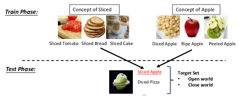
Figure 1: CZSL setting: given the element concepts of sliced and apple, our target is to recognize the compositional concept sliced apple.

In this paper, we investigate the compositional zero-shot learning (CZSL) problem as shown in the example. It requires agents to recognize novel compositions of the attribute-object (attr-obj) pairs appearing in an image by composing previously learned element concepts (e.g., “sliced” and “apple” individually are considered as element concepts). The main challenges of CZSL are 1) zero-shot setting in which we do not have training data for the novel compositions. 2) the model should learn the compositional rules to compose the learned element concepts. 3) the distribution shift from the training data to the test data cased by zero-shot setting. Such shift causes the learned models overfitting the seen compositions and makes it difficult to generalize to novel compositions. Previous solutions usually construct a shared embedding space to calculate the matching scores between images and seen pairs and add different generalizing constraints to regularize the space expecting the learnt embeddings capable of encoding compositional properties [19, 18, 14]. Given impressive performance of large VLMs on downstream tasks, in this work, we attempt to solve CZSL from the lens of prompting large VLMs specifically using CLIP [23] as in [20].

Different from traditional zero-shot learning (ZSL) settings where each class is represented by a single text label [35, 36], CZSL needs to consider the compositional information among the concepts. Therefore, the prompt design which can efficiently encode the compositional information is the main challenge for our work. We expect the designed prompt can re-program CLIP for compositional learning [27] and the compositional labels in the prompt should consider the compositonal information. Motivated by above expectations, we propose GIPCOL (Graph-Injected Soft Prompting for COmpositional Learning) to design a better prompt to apply VMLs in CZSL. The core idea of GIPCOL is to re-program CLIP for CZSL by setting the prefix vectors in the soft prompt as learnable parameters which is different from CSP [20]. Moreover, GIPCOL captures the compositional structure between concepts by constructing a compositional graph from the seen pairs in the training dataset. The concepts, both element concept and compositional concept, are acting as nodes in the graph and the compositional graph models the feasible topological combinations between these concepts. GIPCOL uses a GNN module to update the element label’s representations based on their neighbor information in the constructed compositional graph. And the updated element embedding is used as class labels int the soft prompt. Concretely, the learnable prefix vectors and GNN-updated element concepts consist of the soft prompt for GIPCOL and work together to explore CLIP’s knowledge for CZSL. The contributions of this work can be summarized as follows,

• Novel prompting design. Our technique introduces a novel way of utilizing the compositional structure of concepts for constructing the soft prompts. Though we use GNN for capturing this structure, any other differentiable architectures can be used here to enrich the prompt’s compositional representation.

• GIPCOL achieves SoTA AUC results on all three CZSL benchmarks, including MIT-States, UT-Zappos, and the more challenging C-GQA datasets. Moreover, it shows consistent improvements compared to other CLIP-based methods on all benchmarks.

2 Related Work

Compositional Zero-Shot Learning (CZSL) is a special field of Zero-Shot Learning (ZSL). The CZSL is a challenging problem as it requires generalization from seen compositions to novel compositions by learning the compositional rules between element concepts. There are mainly four lines of research to address this problem. 1) Classifier-based methods train classifiers for attributes and objects separately and combine the element predictions for compositional predictions [16]. 2) Embedding-based methods construct a shared embedding space for both textual pairs and images. Different methods add different constraints on the space to enhance compositionality [19]. 3) Generation-based methods learn to generate visual features for the novel compositions and train classifiers from the generated images [31]. 4) Newly proposed prompt-based methods utilize CLIP and introduce learnable element concept embedding or soft prefix vectors in the soft prompt to solve CZSL problems [20, 32].

Prompt-based Learning. Parallel to ’fine-tuning’, prompt learning provides an efficient mechanism to adapt large pretrained language models(PLMs) or vision-language models (VLMs) to downstream tasks by treating the input prompt as learnable parameters while freezing the rest of the foundation model. Prompt learning is a parameter-efficient framework originated from the NLP field aiming at utilizing knowledge encoded in PLMs for downstream tasks  [13, 2, 24]. Recently, as the prevalence of large vision-language models (VLMs), prompt learning is introduced into multimodal settings to solve VL-related problems [28, 33, 8], including the CZSL problems [20, 32]. In both linguistic and multi-modal settings, prompt engineering plays an important role. How to design a suitable prompt template for downstream tasks is a challenge and GIPCOL proposes a novel approach to address this challenge.

Vision-Language Models. Large VMLs are pre-trained to learn the semantic alignment between vision and language modalities in different levels [7, 23]. Attention-based encoder, large mini-batch contrastive loss, and web-scaled training data are the main factors to boost the performance of such vision-language models. Recent advances in these pre-trained VLMs have presented a promising direction to promote open-world visual understanding with the help of language. Besides the open-world image classification, VLMs are used in other visual fields, like dense prediction [25] and caption generation [17].

Among existing methods, the most relevant to ours are CSP [20] and CGE[18]. CSP treat the element concept labels as learnable parameters to prompt CLIP for CZSL and can be considered as a baseline for GIPCOL. CGE encodes compositional concepts using GNN and constructs a shared embedding space to align images and compositional concepts. It is a task-specific architecture and needs to fine-tune the visual encoder to achieve satisfactory performance. Compared with such task-specific models, GIPCOL is a general prompting method and uses GNN to capture interactions among the concepts for its soft prompting design. GIPCOL fixes CLIP’s pre-trained visual and textual encoders and achieves better performance in a more general and parameter-efficient manner. It is worth noting that GNN used in CGE and GIPCOL have different nature, CGE for compositional encoding and GIPCOL for soft prompt construction.

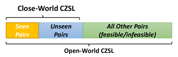
Figure 2: Illustration of different CZSL settings based on the target compositional set. GIPCOL is evaluated under closed-world and open-world settings.

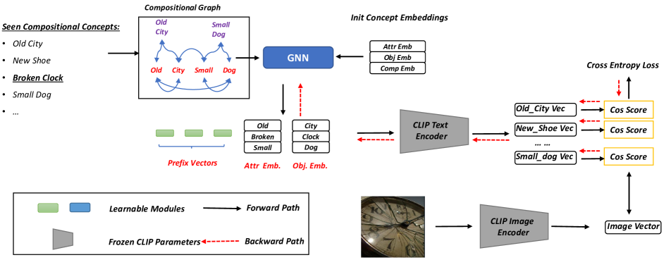
Figure 3: GIPCOL Architecture. Besides CLIP’s frozen text and visual encoders, GIPCOL consists of two learnable components: a soft-prompting module and a GNN. GIPCOL calculates the cosine similarity between the given image and all candidate pairs and the cross-entropy loss is back-propagated through the frozen LM in order to update soft-prompt and GNN.

3 Problem Formulation

In this section, we formally define the CZSL task. Let $\mathbb{A}=\left\{a_{0},a_{1},\ldots,a_{n}\right\}$ be the attribute set and $\mathbb{O}=\left\{o_{0},o_{1},\ldots,o_{m}\right\}$ be the object set. All possible compositional label space $\mathbb{C}$ is the Cartesian product of these two element concept sets, $\mathbb{C}=\mathbb{A}\times\mathbb{O}$ with size $n\times m$. At training time, we are given a set of seen examples $\mathbb{C}_{\text{seen }}=\left\{\left(x_{1},c_{1}\right),\ldots,\left(x_{k},c_{k}\right)\right\}$, where $x_{i}$ is an image and $c_{i}=(a_{i},o_{i})$ is its compositional label from the seen set $\mathbb{C}_{seen}\subset\mathbb{C}$. The goal of CZSL is to learn a function $f$ to assign a compositional label from the target set $\mathbb{C}_{target}\subseteq\mathbb{C}$ to a given image . Based on different target set settings as shown in Fig. 2, CZSL can be categorized into 1) Closed-world CZSL, where $\mathbb{C}_{target}=\mathbb{C}_{seen}\cup\mathbb{C}_{unseen}$, the target set consists of both seen and unseen pairs as introduced in [22]. In this setting, both seen and unseen pairs are feasible. This setting is called a closed-world setting because the test pairs are given in advance. 2) Open-world CZSL, where $\mathbb{C}_{target}=\mathbb{C}$. The target set contains all attr-obj combinations including both feasible and infeasible pairs. This is the most challenging case introduced in [14]. We evaluate our models under both closed-world and open-world settings.

4 GIPCOL

By pre-training on $400$ million image-text association pairs, CLIP has already learned the general knowledge for images recognition. In order to fully utilize CLIP’s capability in compositional learning, GIPCOL freezes CLIP’s textual and visual encoders and focuses on structuring its textual prompt to address compositional concept learning. The GIPCOL’s architecture is shown in Fig. 3. In particular, GIPCOL adds two learnable components to construct the soft prompt for CZSL: the learnable prefix vectors and the GNN module. The prefix vectors are used to add more learnable parameters to represent the compositional concepts and reprogram CLIP for compositional learning. The GNN module is to capture the compositional structure of the objects and attributes for a better compositional concept representation in the constructed soft prompt. We describe the details of GIPCOL, including the learnable prefix vectors, GNN, and CLIP’s visual/textual encoder in the following section.

4.1 GIPCOL Architecture

Learnable Prefix Vectors. We designate $k$ learnable prefix vectors $\Theta=\{\theta_{1},\theta_{2},...,\theta_{m}\}$ where $\theta_{i}\in\mathbb{R}^{d}$ in soft prompt for compositional concept encoding. $d$ is set to $768$ to be consistent with CLIP embedding size. Here, larger $k$ means more learnable parameters and learning ability for compositional concept representation. These vectors are used to prepend to the attr-obj embeddings and act as part of the compositional representation. These prefix vectors are fine-tuned by gradients flowing back through CLIP during the training time.

GNN as Concept Encoder. Different from traditional zero-shot learning (ZSL) problems where output labels are treated independently, CZSL requires modeling the interactions between element concepts. For example, given the compositional concept red apple, we need to learn both the concept apple and how red changes apple’s state instead of treating red and apple as two independent concepts. Graph Neural Networks (GNN) have been proved to be able to capture such dependencies [18, 15]. We introduce GNN in GIPCOL to enrich the concept’s representations by fusing information from their compositional neighbors as follows,

$$(\hat{a_{i}},\hat{o_{i}})=GNN_{\Phi}(a_{i},o_{i})$$ (1)

where $\Phi$ is GNN’s parameter, $(a_{i},o_{i})$ and $(\hat{a_{i}},\hat{o_{i}})$ are the original and updated compositional concept’s representation. The updated node representations from GNN will serve as class labels in soft prompt. The whole soft prompt represents the compositional concept and will be put into CLIP’s textual encoder for compositional learning.

Frozen CLIP’s Text Encoder. After obtaining the updated compositional representations $(\hat{a_{i}},\hat{o_{i}})$, GIPCOL adds the learnable prefix vectors $\Theta=[\theta_{1},\theta_{2},...,\theta_{m}]$ prepending in front of $(\hat{a_{i}},\hat{o_{i}})$ to represent compositional concept as follows,

$$[\underbrace{SOS,\hskip 10.0pt\overbrace{\theta_{1},\theta_{2},...,\theta_{m}}^{\textbf{prefix Vectors}},\hskip 4.0pt\overbrace{\hat{a_{i}},\hat{o_{i}},}^{\textbf{GNN-Updated Concept}}EOS}_{\textbf{Soft Prompt \noindent as Compositional Concept Representation}}].$$ (2)

Then we use CLIP’s frozen text encoder, a Bert encoder [5], to extract the normalized EOS vector as the compositional concept’s representation for further multi-modal alignment as follows,

$$\boldsymbol{c}_{i}=\frac{TxtEnc\left({\Theta,(\hat{a_{i}},\hat{o_{i}})}\right)}{\left\|TxtEnc\left(\Theta,(\hat{a_{i}},\hat{o_{i}})\right)\right\|}$$ (3)

where $(\hat{a_{i}},\hat{o_{i}})$ is the GNN-updated attribute and object vectors and $c_{i}$ is the $i$-th compositional concept vector encoded by CLIP.

Frozen visual encoder. Following CLIP’s pre-processing routine, we first rescale the image’s size to $224\times 224$. Then we use ViT-L/14 as the visual encoder ViT to encode the image and extract the [CLASS] token as the image’s representation. The extracted image vector $x_{i}$ needs to be normalized as follows for further similarity calculation.

$$\boldsymbol{x}_{i}=\frac{VisEnc(v_{i})}{\left\|VisEnc(v_{i})\right\|}$$ (4)

where $v_{i}$ is the given image and $x_{i}$ is its vector representation.

Aligning Image and Compositional Concept. After obtaining the vectors for the compositional concept $c_{i}$ and the image $x$, GIPCOL calcualtes the probability of $x$ belonging to class $c_{i}$ as follows,

$$p(c_{i}\mid x)=\frac{\exp\left(\left(x\cdot c_{i}\right)/\tau\right)}{\sum_{k=1}^{K}\exp\left(\left(x\cdot c_{k}\right)/\tau\right).}$$ (5)

where $\tau$ is a temperature parameter from CLIP, $\cdot$ denotes the inner product of the concept vector and the image vector and $K$ is the number of attr-obj pairs in the training set.

4.2 GNN in Soft Prompting

As disussed previously, a key idea to address the CZSL problem is to learn concept representations that are able to internalize the compositional information. Graph could be the tool to model such compositional dependencies. And this idea has been used in previous work [18, 15] by applying Graph Neural Networks(GNN) as encoders to represent the compositional concepts. Although we adopt similar graph-based methods for compositional encoding, our novelty is to use the graph’s compositional structure to facilitate the automated prompt engineering in compositional learning as shown in Appendix A. We model the element concepts and their composition explicitly in GNN for the soft prompting construction. In principle, the GNN module can be replaced by other differentiable architectures that are able to capture the concept’s compositional information. We describe the detailed GNN application in GIPCOL next.

Node Embedding $\mathcal{V}$. There are two types of nodes in GIPCOL’s compositional graph: element concept node and compositional concept node. The node embedding’s size is $R^{(|a|+|o|+|c|)*d}$, where $|a|$ is the attribute number, $|o|$ is the object number, $|c|$ is the training pair number and $d$ is the feature dimension. For the element nodes, we initialize them using CLIP’s embedding vectors. For the compositional nodes, we initialize them using the average embedding of the element nodes, that is, $\frac{att\_vec+obj\_vec}{2}$. GIPCOL relies on GNN to fuse information from the constructed compositional graph and update the concept’s representation.

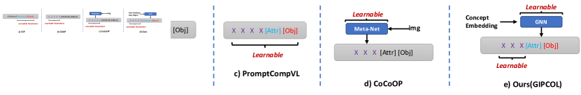
Figure 4: Different prompting strategies. GIPCOL combines both soft prefix vector and GNN for prompt construction.

Compositional Graph Constructions $\mathcal{E}$. We use a graph to capture the compositional dependencies and learn richer concept representations. The connection design among concepts is the key challenge for such graph. In order to utilize the feasible compositional information, GIPCOL considers the training pairs and construct one single compositional graph for both closed-world CZSL and open-world CZSL to conserve the computing and storage resources. Specifically, given a pair $c=(a,o)$, besides the self-connected edge, GIPCOL adds three undirected edges $(c\leftrightarrow a)$, $(c\leftrightarrow o)$ and $(a\leftrightarrow o)$ in the graph where the adjacency matrix $A\in\mathbb{R}^{K\times K}$ is symmetric with $K=|a|+|o|+|c|$. The compositional concept plays the bridging role to help connect element concepts and only the element concepts are used to construct the compositional prompting due to the zero-shot setting.

GNN Module: Once we have the compositional graph and the initialized concept features, we can update the concept’s embedding by fusing the compositional information from its neighbors. Any GNN models could be applied here and in GIPCOL, we use Graph Convolution Network (GCN) [10] in Eq. 6 for compositional encoding.

$$H^{(l+1)}=\sigma\left(\tilde{D}^{-\frac{1}{2}}\tilde{A}\tilde{D}^{-\frac{1}{2}}H^{(l)}\Phi^{(l)}\right)$$ (6)

where $H^{l}$ denotes the node’s representations in the $l^{th}$ layer, $\sigma$ is the non-linearity ReLU function, $\tilde{A}$ is the adjacency matrix with added self-connections, $\tilde{D}$ is a diagonal node degree matrix and $\Phi^{l}$ is the learnable weight matrix in layer $l$. Notably, other graph constructing methods, like using external knowledge [9], and other GNN models, like GAT [29], could be further explored to improve CZSL performance based on GIPCOL’s architecture. However, these are not target of this work. Here, GIPCOL shows the effectiveness of utilizing compositional knowledge in prompting construction in CZSL.

4.3 Training

After obtaining the concept and image representations, we calculate the class probability using Eq. 5. And the regularized Cross-Entropy loss is used to update GIPCOL’s prefix vectors $\Theta$ and GNN parameters $\Phi$ as follows,

$$-\frac{1}{\left|\mathbb{N}\right|}\sum_{i\in\mathbb{N}}\log p_{\boldsymbol{\theta}}(c_{i}\mid x)+\lambda_{1}\|\boldsymbol{\Theta}\|^{2}+\lambda_{2}\|\boldsymbol{\Phi}\|^{2}$$ (7)

where $\lambda_{1}$ and $\lambda_{2}$ are the hyper-parameters to control the weight decay for prefix vector and GCN separately. GIPCOL keeps CLIP’s pre-trained textural and visual encoders fixed during the training time. And more details about the training process can be found in Append. B.

4.4 Inference

During inference, given an image, we first construct the soft prompts for all target concepts using the fine-tuned prefix vectors and GNN. Then, we use CLIP’s frozen textual and visual encoders to obtain the image vector $x$ and the target concept vector set $\mathbb{C}_{tareget}$. Then we use cosine measurement to select the most similar attr-obj pair from $\mathbb{C}_{target}$ as the compositional label as follows,

$$\hat{c}=\underset{c_{i}\in\mathbb{C}_{\text{target}}}{\arg\max}\ cos\left(c_{i},x\right).$$ (8)

where $c_{i}$ is the $i$-th compositional vector from the target set.

4.5 CLIP-Prompting Method Comparison

In this section, we clarify the difference between all CLIP-prompting methods used in CZSL as shown in Fig. 4. Generally, all current CLIP-prompting methods keeps the image representation fixed and learn constructing the CLIP’s textual prompt to represent the compositional concept as shown in Eq. 2. The main difference is that CSP[20] learns the element embedding, COOP[35] learns the prefix vectors and PromptCompVL learns both the element embedding and the prefix vectors. All these three methods do not explicit consider the compositional structures between concepts. In order to inject more semantic information into soft prompt, CoCoOP[36] introduces a Meta-Net and tries to modify the prefix vectors based on each image input. It uses the instance-level information not the global compositional information for CZSL. Such instance-level prompting also causes training inefficient and consumes a significant amount of computing resources as discussed in that work. Different from all previous methods, GIPCOL proposed a novel prompting strategy by combining the learnable prefix vectors and the GNN module and the detailed comparition is in Append. A.

5 Experiments

5.1 Experimental Setting

Datasets. We conduct experiments on three datasets, MIT-States [6] UT-Zappos [34] and C-GQA [18]. MIT-States and C-GQA consist of images with objects and their attributes in the general domain. In contrast, UT-Zappos contains images of shoes paired with their material attributes which is a more domain-specific dataset. Our experiments follow the previous works [22, 18] on the data split for training and testing. More details about the data splits and statistics can be found in Append. C.

Implementation details. We extend on the codebase of [20] and  [18] for GIPCOL’s implementation. Moreover, for a fair comparison, the length of the prefix vector, $k$, is set to $3$ which is the same length of CLIP hard-prompting ’a photo of’. The dimension of soft-prompting $d$ is set to $768$ which is consistent with CLIP’s model setting. Moreover, we use two-layer GCN to encode concepts and the corresponding GNN’s learnable parameters are $\Phi=\{\Phi^{1},\Phi^{2}\}$ Our code will be made publicly available on GitHub.

Evaluation Metrics. Zero-shot models are biased to the seen classes as shown in previous woks [4, 14]. As a standard method in zero-shot learning, we introduce a scalar value adding to the unseen classes to adjust the bias towards the seen classes as used in [22, 20]. By varying the added bias from $-\infty$ to $+\infty$, we report GIPCOL’s performance using the following four metrics in both the closed-world and the open-world settings as discussed in Sec. 3: 1) Best seen accuracy (S), testing only on seen compositions when bias is $-\infty$; 2) Best unseen accuracy (U), testing only on unseen compositions when bias is $+\infty$; 3) Best harmonic mean (HM) which balances the performance between seen and unseen accuracies; 4) Area Under the Curve (AUC), the area below the seen-unseen accuracy curve by varying the scalar added to the unseen compositional concepts.

Baselines. We compare GIPCOL with two types of baselines: 1) non-CLIP methods (top seven models in the closed setting and top six in the open setting) namely Attributes as Operators (AoP)[19], Label Embed+ (LE+)[16], Task Modular Networks (TMN)[22], SymNet[12], Compositional Graph Embeddings (CGE)[18], Compositional Cosine Logits (CompCos)[14] and Siamese Contrastive Embedding Network(SCEN)[11]. 2) CLIP-based methods (the bottom three models), namely CLIP[23], Context Optimization(COOP)[35] and compositional soft prompting (CSP)[20].

	MIT-States				UT_Zappos				C-GQA
Method	S	U	H	AUC	S	U	H	AUC	S	U	H	AUC
AoP [19]	14.3	17.4	9.9	1.6	59.8	54.2	40.8	25.9	17.0	5.6	5.9	0.7
LE+ [16]	15.0	20.1	10.7	2.0	53.0	61.9	41.0	25.7	18.1	5.6	6.1	0.8
TMN [22]	20.2	20.1	13.0	2.9	58.7	60.0	45.0	29.3	23.1	6.5	7.5	1.1
SymNet [12]	24.2	25.2	16.1	3.0	49.8	57.4	40.4	23.4	26.8	10.3	11.0	2.1
CompCos [14]	25.3	24.6	16.4	4.5	59.8	62.5	43.1	28.7	28.1	11.2	12.4	2.6
CGE [18]	32.8	28.0	21.4	6.5	64.5	71.5	60.5	33.5	33.5	15.5	16.0	4.2
SCEN [11]	29.9	25.2	18.4	5.3	63.5	63.1	47.8	32.0	28.9	25.4	17.5	5.5
CLIP [23]	30.2	40.0	26.1	11.0	15.8	49.1	15.6	5.0	7.5	25.0	8.6	1.4
COOP [35]	34.4	47.6	29.8	13.5	52.1	49.3	34.6	18.8	20.5	26.8	17.1	4.4
CSP [20]	46.6	49.9	36.3	19.4	64.2	66.2	46.6	33.0	28.8	26.8	20.5	6.2
GIPCOL (Ours)	48.5	49.6	36.6	19.9	65.0	68.5	48.8	36.2	31.92	28.4	22.5	7.14

Table 1: Closed-World CZSL results on UT-Zappos, Mit-States and C-GQA datasets.

	MIT-States				UT_Zappos				C-GQA
Method	S	U	H	AUC	S	U	H	AUC	S	U	H	AUC
AoP [19]	16.6	5.7	4.7	0.7	50.9	34.2	29.4	13.7	-	-	-	-
LE+ [16]	14.2	2.5	2.7	0.3	60.4	36.5	30.5	16.3	19.2	0.7	1.0	0.08
TMN [22]	12.6	0.9	1.2	0.1	55.9	18.1	21.7	8.4	-	-	-	-
SymNet [12]	21.4	7.0	5.8	0.8	53.3	44.6	34.5	18.5	26.7	2.2	3.3	0.43
CompCos [14]	25.4	10.0	8.9	1.6	59.3	46.8	36.9	21.3	-	-	-	-
CGE [18]	32.4	5.1	6.0	1.0	61.7	47.7	39.0	23.1	32.1	1.8	2.9	0.47
CLIP [23]	30.1	14.3	12.8	3.0	15.7	20.6	11.2	2.2	7.5	4.6	4.0	0.27
COOP [35]	34.6	9.3	12.3	2.8	52.1	31.5	28.9	13.2	21.0	4.6	5.5	0.70
CSP [20]	46.3	15.7	17.4	5.7	64.1	44.1	38.9	22.7	28.7	5.2	6.9	1.20
GIPCOL (Ours)	48.5	16.0	17.9	6.3	65.0	45.0	40.1	23.5	31.6	5.5	7.3	1.30

Table 2: Open-World CZSL results on UT-Zappos, Mit-States and C-GQA datasets.

Feasibility Calibration in Open-World Setting. Open-world CZSL is more challenging compared with the closed-world setting as the class space contains all possible combinations of attributes and objects including both feasible compositions and infeasible compositions. In order to filter out the infeasible compositions, we apply the feasibility calibration as used in [14, 20]. For each unseen pair $(a,o)$, we first collect two sets from the training data. One is the applicable attribute set $A=\{a_{1},a_{2},\dots,a_{M}\}$ for the target object $o$ and the other is the applicable object set $O=\{o_{1},o_{2},\dots,o_{N}\}$ for the target attribute $a$ where $(a_{i},o)$ and $(a,o_{j})$ has been observed in training time. Then we calculate the similarity between $a$ and each element in $A$ and use the maximum similarity score as this pair’s attribute feasibility score as follows,

$$f_{a}(a,o)=\max_{(a_{i},o)\in\mathbb{C}_{\text{seen }}}\frac{e(a)\cdot e(a_{i})}{\|e(a)\|\|e(a_{i})\|},$$ (9)

where $e$ is the GloVe embedding [21]. On the other hand, this pair’s object feasibility score is calculated in a similar way based on the applicable object set. Finally, the unseen pair feasibility score is calculated as the average of the two scores, $\frac{f_{a}+f_{o}}{2}$. After obtaining the feasibility score for all unseen pairs, we can filter out infeasible compositions by setting a threshold $T$ whcih can be tuned based on the validation set. The final prediction for image $x$ in the open-world setting is computed as follows,

$$\hat{c}=\underset{c_{i}\in\mathbb{C}_{\text{target}},\hskip 2.0ptc_{i}\geq T}{\arg\max}\ cos\left(c_{i},x\right).$$ (10)

Different from the closed-world setting, we require the feasibility score of the predicted label $c$ to be larger than a threshold. The threshold uses in our experiments is shown in Append. D.

5.2 Results

Results on MIT-States. As shown in Tab. 1 and 2, GIPCOL achieves the new SoTA results on MIT-States on both closed-world and open-world settings compared with CLIP and non-CLIP baselines (except for the best-unseen metric (U)). The CLIP-based models have consistently better performance compared to the non-CLIP methods. CLIP-prompting methods, including COOP, CSP and ours, further boost the performance compared to the vanilla CLIP model.

Results on UT-Zappos. On UT-Zappos, previous CLIP-based approaches under-perform the SoTA performance achieved by CGE which is a non-CLIP model. However, GIPCOL successfully surpasses the CGE model. Note that UT-Zappos is a domain-specific dataset that consists of shoe types and the materials. We suspect that CLIP may not have seen sufficient similar samples from this specific domain and therefore purely tuning the prompting is not helpful to solve the problem. In contrast, GIPCOL adds additional compositional information to learn the element concept embedding which appears to boost the compositional learning ability within this specific domain.

Results on C-GQA. On the more challenging C-GQA dataset, GIPCOL also achieves new SoTA results on both closed and open world settings with an exception for the seen accuracy in the open world. However, the key metric is AUC which is consistently higher for GIPCOL in all settings.

5.3 Qualitative Analysis

Predicted Examples. We looked into a number of randomly selected predictions from GIPCOL shown in Append. E. The red colored texts are the ground-truth labels, the blue colored texts are GIPCOL’s correctly predicted labels and the black colored texts are GIPCOL’s wrongly predicted labels. The first two columns present examples with correctly predicted compositional labels and the last two columns show the wrongly predicted labels, either wrong in attributes or wrong in objects. From this figure, we can see that GIPCOL can recognize objects in most of the compositions in MIT-States and C-GQA datasets. However, it has difficulty to precisely predict the attributes for these two datasets. For example, it predicts modern clock instead of ancient clock which is the antonym of the actual attribute. But for UT-Zappos, the more domain-specific dataset, GIPCOL even has difficulty in recognizing the objects.

Differences in Domains: From Tables 1 and 2, we observe that CLIP without any prompt-tuning can achieve better performance compared to non-CLIP models on the MIT-States dataset, but not on the UT-Zappos dataset. We hypothesize that this issue can be related to the distribution difference between the pre-training data used by CLIP and the data domain of the downstream task. To validate this hypothesis, we further look into some concrete examples from MIT-stats and UT-Zappos. We take burnt boat from MIT-Stats and Faux Fur-Shoes Clogs and Mules from UT-Zappos for comparison as shown in Append. F. The CLIP’s training data is not publicly available. However, LAION-400M [26] used the released CLIP model and obtained the closest 400M image-text pairs from their crawled dataset from Web by reverse engineering. We based our analysis on this constructed LAION-400M subset. By querying LAION-400M with burn boat, we could retrieve about $600$ relevant images. By querying with Faux Fur_Shoes Clogs and Mules we can retrieve about $200$ relevant images. The first interesting difference is in the quantity of the retrieved relevant images which is significantly lower for the shoe dataset. The second difference is the data quality differences. As can be seen from Append. F, the retrieved shoes are less similar to the UT-Zappos’ shoes when compared to the similarity of the retrieved boats to MIT-Stats boats. We note that UT-Zappos is about shoe fashion and was constructed in 2014 while CLIP is pretrained using recent 2020’s images. The change in fashion trends has made the images look different for the same compositional concept. Based on these observations, it is evident that the quantity and quality of CLIP’s pre-training data play an important role in its performance.

Covering the Performance Gap. Despite the above-mentioned issues, GIPCOL improves the UT-Zappos dataset. While we found that CLIP’s pre-training data is important in its performance in the Zero-shot setting, introducing the additional compositional knowledge in GIPCOL positively impacts CLIP’s ability in recognizing the novel compositional concepts. GIPCOL uses GNN to inject compositional information into concept representations which turned out to be helpful. The improvement is important, especially for UT-Zappos which is a special domain with not many shared similar examples with CLIP’s training.

5.4 Ablation Study

To better understand the influence of each component in GIPCOL, Tab. 3 shows the performances of its variations on UT-Zappos’ closed-world setting.

Model	S	U	H	AUC
GIPCOL	65.0	68.5	48.8	36.2
- without GNN	64.4	64.0	46.12	32.2
- without prefix	64.7	62.3	45.9	31.0
- without both (CLIP)	15.8	49.1	15.6	5.0

Table 3: Performance of GIPCOL’s variations.

Effects of GNN. We remove the GNN module and directly set attribute and object embeddings as learnable parameters as in [32]. The performance decreases. Especially the AUC drops from $36.2\%$ to $32.2\%$.

Effect of Learnable Prefix Vectors. Another variant of GIPCOL is to fix the prefix vectors and only tune the GNN module to update the class embeddings. From Tab. 3, we can see that learnable prefix vectors play a more important role than GNN. In fact, adding the prefix vectors changes CLIP’s textual input and makes it biased towards compositional learning, which is a key component in GIPCOL.

5.5 Higher-Order Compositional Learning

Previous work (CSP) [20] introduced another challenging dataset: AAO-MIT-States, a subset derived from MIT-States to evaluate the higher-order compositional learning ability in the form of attribute-attribute-object (AAO) compositions. After learning the prefix vectors and GNN-encoded element concepts, GIPCOL can be easily adapted to solve AAO by modifying the compositional prompt to $(\theta_{1},\theta_{2},...,\theta_{m},\hat{a_{i}},\hat{a_{j}},\hat{o_{k}})$ to represent the higer-order compositions. We report the AAO results in Tab. 4. We can see that GIPCOL has a better higher-order compositional leaning ability, with a $3\%$ absolute improvement compared with CSP.

Model	Accuracy
CLIP	62.7
CSP	72.6
GIPCOL (Ours)	75.9

Table 4: AAO Performance of different CLIP-based models.

6 Conclusion

In this paper, we propose GIPCOL, a new CLIP-based prompting framework, to address the compositional zero-shot learning (CZSL) problem. The goal is to recognize compositional concepts of objects with their states and attributes as described by images. The objects and attributes have been observed during training in some compositions, however, the test-time compositions could be novel and unseen. We introduce a novel prompting strategy for soft prompt construction by treating element concepts as part of a global GNN network that encodes feasible compositional information including objects, attributes and their compositions. In this way, the soft-prompt representation is influenced not only by the pre-trained VLMs but also by all the compositional representations in its neighborhood captured by the compositional graph. Our results have shown that GIPCOL performs better and achieves SoTA AUC results on all three benchmarks including MIT-States, UT-Zappos, and C-GQA . These results demonstrate the advantages and limitations of prompting large vision and language models (such as CLIP) for compositional concept learning.

Appendix A Comparison between GIPCOL and CGE

Although both CGE[18] and GIPCOL use GNN to encode compositional concepts, the GNN module functions in a fundamentally different manner in these two models. GNN in GIPCOL helps construct the soft prompting for CZSL. However, GNN in CGE plays the text encoder role which projects the concept into the embedding space. GIPCOLL freeze CLIP’s textual and visual encoders to utilize CLIP’s multi-modal aligning ability for CZSL which is more efficient. In contrast, CGE needs to train both the GNN and visual encoder to obtian competitive performance as compared in Fig. 5.

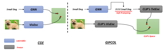
Figure 5: Comparison between CGE and GIPCOL. GIPCOL uses GNN to help prompt construction.

Appendix B GIPCOL Algorithm

1:Initialize GIPCOL using CLIP’s pre-trained textual and visual encoders.

2:Update element concept’s representation using GNN as Eq. 1 and Eq. 6.

3:Construct textual prompt for compositional labels using the updated element concepts and learnable prefix vectors as Eq. 2.

4:Extract and normalize image/text vectors using CLIP’s image/text encoder using Eq. 3 and Eq. 4 seperately.

5:Calculate the class probability as Eq. 5 using the cosine similarity and update GIPCOL’s soft-prompting layer $\Theta$ and GNN layer $\Phi$ using Cross-Entropy loss.

Algorithm 1 GIPCOL

Appendix C CZSL Dataset Statistics

	MIT-States	UT-Zappos	C-GQA
# $Attr.$	$115$	$16$	$413$
# $Obj.$	$245$	$12$	$674$
# $Attr.\times Obj.$	$28175$	$192$	$278362$
# Train Pair	$1262$	$83$	$5592$
# Train Img.	$30338$	$22998$	$26920$
# Val. Seen Pair	$300$	$15$	$1252$
# Val. Unseen Pair	$300$	$15$	$1040$
# Val. Img.	$10420$	$3214$	$7280$
# Test Seen Pair	$400$	$18$	$888$
# Test Unseen Pair	$400$	$18$	$923$
# Test Img.	$19191$	$2914$	$5098$

Table 5: Dataset Statistics for MIT-States, UT-Zappos and C-GQA.

Appendix D Feasible Score Threshold in Open-World CZSL

In open-world CZSL (OW-CZSL), we use the validation set to choose a feasible threshold to remove less feasible compositions from the output space and the adopted threshold in GIPCOL is shown in Tab. 6.

Dataset	Feasibility Score
MIT-States	0.40691
UT-Zappos	0.51878
C-GQA	0.49941

Table 6: GIPCOL’s feasibility threshold score.

Appendix E Qualitative Examples

Figure 6: We show the top-3 predictions of our proposed model for some images. Red colors are ground-truth labels, blue colors are correctly predicted labels and black colors are wrongly predicted labels.

Appendix F Comparison between CLIP’s Pre-train Dataset and Target Dataset

We visualize CLIP’s pre-training dataset and target domain dataset in Fig. 7. From this figure, we can see that MIT-States have similar visual appearance with CLIP’s pre-trained data. However, for UT-Zappos, because of the fashion style change overtime, shoes have significant visual appearance between the pre-training dataset and the target dataset. Results in Tab. 1 and Tab. 2 have shown the domain similarity plays an important role in prompting-based method. Prompting CLIP without any training can achieve better performance on MIT-State then UT-Zappos. GIPCOL helps address this challenge partially by prompting design based on the restuls.

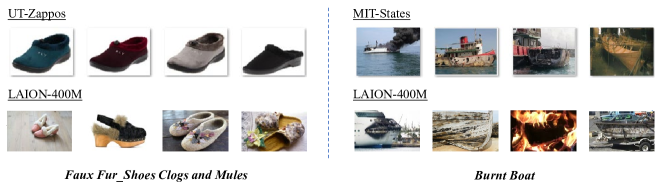
Figure 7: Comparison between retrieved images from Laion400M and UT-Zappos/MIT-States.

References

- [1] Peter Anderson, Qi Wu, Damien Teney, Jake Bruce, Mark Johnson, Niko Sünderhauf, Ian Reid, Stephen Gould, and Anton Van Den Hengel. Vision-and-language navigation: Interpreting visually-grounded navigation instructions in real environments. In Proceedings of the IEEE conference on computer vision and pattern recognition, pages 3674–3683, 2018.
- [2] Tom Brown, Benjamin Mann, Nick Ryder, Melanie Subbiah, Jared D Kaplan, Prafulla Dhariwal, Arvind Neelakantan, Pranav Shyam, Girish Sastry, Amanda Askell, et al. Language models are few-shot learners. Advances in neural information processing systems, 33:1877–1901, 2020.
- [3] Joyce Y Chai, Qiaozi Gao, Lanbo She, Shaohua Yang, Sari Saba-Sadiya, and Guangyue Xu. Language to action: Towards interactive task learning with physical agents. In IJCAI, pages 2–9, 2018.
- [4] Wei-Lun Chao, Soravit Changpinyo, Boqing Gong, and Fei Sha. An empirical study and analysis of generalized zero-shot learning for object recognition in the wild. In Computer Vision–ECCV 2016: 14th European Conference, Amsterdam, The Netherlands, October 11-14, 2016, Proceedings, Part II 14, pages 52–68. Springer, 2016.
- [5] Jacob Devlin, Ming-Wei Chang, Kenton Lee, and Kristina Toutanova. Bert: Pre-training of deep bidirectional transformers for language understanding. arXiv preprint arXiv:1810.04805, 2018.
- [6] Phillip Isola, Joseph J Lim, and Edward H Adelson. Discovering states and transformations in image collections. In Proceedings of the IEEE conference on computer vision and pattern recognition, pages 1383–1391, 2015.
- [7] Chao Jia, Yinfei Yang, Ye Xia, Yi-Ting Chen, Zarana Parekh, Hieu Pham, Quoc Le, Yun-Hsuan Sung, Zhen Li, and Tom Duerig. Scaling up visual and vision-language representation learning with noisy text supervision. In International Conference on Machine Learning, pages 4904–4916. PMLR, 2021.
- [8] Woojeong Jin, Yu Cheng, Yelong Shen, Weizhu Chen, and Xiang Ren. A good prompt is worth millions of parameters? low-resource prompt-based learning for vision-language models. arXiv preprint arXiv:2110.08484, 2021.
- [9] S Karthik, M Mancini, and Zeynep Akata. Kg-sp: Knowledge guided simple primitives for open world compositional zero-shot learning. 2022.
- [10] Thomas N Kipf and Max Welling. Semi-supervised classification with graph convolutional networks. arXiv preprint arXiv:1609.02907, 2016.
- [11] Xiangyu Li, Xu Yang, Kun Wei, Cheng Deng, and Muli Yang. Siamese contrastive embedding network for compositional zero-shot learning. In Proceedings of the IEEE/CVF Conference on Computer Vision and Pattern Recognition, pages 9326–9335, 2022.
- [12] Yong-Lu Li, Yue Xu, Xiaohan Mao, and Cewu Lu. Symmetry and group in attribute-object compositions. In Proceedings of the IEEE/CVF Conference on Computer Vision and Pattern Recognition, pages 11316–11325, 2020.
- [13] Pengfei Liu, Weizhe Yuan, Jinlan Fu, Zhengbao Jiang, Hiroaki Hayashi, and Graham Neubig. Pre-train, prompt, and predict: A systematic survey of prompting methods in natural language processing. arXiv preprint arXiv:2107.13586, 2021.
- [14] Massimiliano Mancini, Muhammad Ferjad Naeem, Yongqin Xian, and Zeynep Akata. Open world compositional zero-shot learning. In Proceedings of the IEEE/CVF Conference on Computer Vision and Pattern Recognition, pages 5222–5230, 2021.
- [15] Massimiliano Mancini, Muhammad Ferjad Naeem, Yongqin Xian, and Zeynep Akata. Learning graph embeddings for open world compositional zero-shot learning. IEEE Transactions on pattern analysis and machine intelligence, 2022.
- [16] Ishan Misra, Abhinav Gupta, and Martial Hebert. From red wine to red tomato: Composition with context. In Proceedings of the IEEE Conference on Computer Vision and Pattern Recognition, pages 1792–1801, 2017.
- [17] Ron Mokady, Amir Hertz, and Amit H Bermano. Clipcap: Clip prefix for image captioning. arXiv preprint arXiv:2111.09734, 2021.
- [18] Muhammad Ferjad Naeem, Yongqin Xian, Federico Tombari, and Zeynep Akata. Learning graph embeddings for compositional zero-shot learning. In Proceedings of the IEEE/CVF Conference on Computer Vision and Pattern Recognition, pages 953–962, 2021.
- [19] Tushar Nagarajan and Kristen Grauman. Attributes as operators: factorizing unseen attribute-object compositions. In Proceedings of the European Conference on Computer Vision (ECCV), pages 169–185, 2018.
- [20] Nihal V Nayak, Peilin Yu, and Stephen H Bach. Learning to compose soft prompts for compositional zero-shot learning. arXiv preprint arXiv:2204.03574, 2022.
- [21] Jeffrey Pennington, Richard Socher, and Christopher D Manning. Glove: Global vectors for word representation. In Proceedings of the 2014 conference on empirical methods in natural language processing (EMNLP), pages 1532–1543, 2014.
- [22] Senthil Purushwalkam, Maximilian Nickel, Abhinav Gupta, and Marc’Aurelio Ranzato. Task-driven modular networks for zero-shot compositional learning. In Proceedings of the IEEE/CVF International Conference on Computer Vision, pages 3593–3602, 2019.
- [23] Alec Radford, Jong Wook Kim, Chris Hallacy, Aditya Ramesh, Gabriel Goh, Sandhini Agarwal, Girish Sastry, Amanda Askell, Pamela Mishkin, Jack Clark, et al. Learning transferable visual models from natural language supervision. In International Conference on Machine Learning, pages 8748–8763. PMLR, 2021.
- [24] Colin Raffel, Noam Shazeer, Adam Roberts, Katherine Lee, Sharan Narang, Michael Matena, Yanqi Zhou, Wei Li, Peter J Liu, et al. Exploring the limits of transfer learning with a unified text-to-text transformer. J. Mach. Learn. Res., 21(140):1–67, 2020.
- [25] Yongming Rao, Wenliang Zhao, Guangyi Chen, Yansong Tang, Zheng Zhu, Guan Huang, Jie Zhou, and Jiwen Lu. Denseclip: Language-guided dense prediction with context-aware prompting. In Proceedings of the IEEE/CVF Conference on Computer Vision and Pattern Recognition, pages 18082–18091, 2022.
- [26] Christoph Schuhmann, Richard Vencu, Romain Beaumont, Robert Kaczmarczyk, Clayton Mullis, Aarush Katta, Theo Coombes, Jenia Jitsev, and Aran Komatsuzaki. Laion-400m: Open dataset of clip-filtered 400 million image-text pairs. arXiv preprint arXiv:2111.02114, 2021.
- [27] Yun-Yun Tsai, Pin-Yu Chen, and Tsung-Yi Ho. Transfer learning without knowing: Reprogramming black-box machine learning models with scarce data and limited resources. In International Conference on Machine Learning, pages 9614–9624. PMLR, 2020.
- [28] Maria Tsimpoukelli, Jacob L Menick, Serkan Cabi, SM Eslami, Oriol Vinyals, and Felix Hill. Multimodal few-shot learning with frozen language models. Advances in Neural Information Processing Systems, 34:200–212, 2021.
- [29] Petar Velickovic, Guillem Cucurull, Arantxa Casanova, Adriana Romero, Pietro Lio, Yoshua Bengio, et al. Graph attention networks. stat, 1050(20):10–48550, 2017.
- [30] Oriol Vinyals, Alexander Toshev, Samy Bengio, and Dumitru Erhan. Show and tell: A neural image caption generator. In Proceedings of the IEEE conference on computer vision and pattern recognition, pages 3156–3164, 2015.
- [31] Yongqin Xian, Tobias Lorenz, Bernt Schiele, and Zeynep Akata. Feature generating networks for zero-shot learning. In Proceedings of the IEEE conference on computer vision and pattern recognition, pages 5542–5551, 2018.
- [32] Guangyue Xu, Parisa Kordjamshidi, and Joyce Chai. Prompting large pre-trained vision-language models for compositional concept learning. arXiv:2211.05077, 2022.
- [33] Zhengyuan Yang, Zhe Gan, Jianfeng Wang, Xiaowei Hu, Yumao Lu, Zicheng Liu, and Lijuan Wang. An empirical study of gpt-3 for few-shot knowledge-based vqa. In Proceedings of the AAAI Conference on Artificial Intelligence, volume 36, pages 3081–3089, 2022.
- [34] Aron Yu and Kristen Grauman. Fine-grained visual comparisons with local learning. In Proceedings of the IEEE Conference on Computer Vision and Pattern Recognition, pages 192–199, 2014.
- [35] Kaiyang Zhou, Jingkang Yang, Chen Change Loy, and Ziwei Liu. Conditional prompt learning for vision-language models. In CVPR, 2022.
- [36] Kaiyang Zhou, Jingkang Yang, Chen Change Loy, and Ziwei Liu. Conditional prompt learning for vision-language models. In IEEE/CVF Conference on Computer Vision and Pattern Recognition (CVPR), 2022.