A Physics-Informed, Deep Double Reservoir Network for Forecasting Boundary Layer Velocity

Matthew Bonas, David H. Richter and Stefano Castruccio¹

Abstract

When a fluid flows over a solid surface, it creates a thin boundary layer where the flow velocity is influenced by the surface through viscosity, and can transition from laminar to turbulent at sufficiently high speeds. Understanding and forecasting the wind dynamics under these conditions is one of the most challenging scientific problems in fluid dynamics. It is therefore of high interest to formulate models able to capture the nonlinear spatio-temporal velocity structure as well as produce forecasts in a computationally efficient manner. Traditional statistical approaches are limited in their ability to produce timely forecasts of complex, nonlinear spatio-temporal structures which are at the same time able to incorporate the underlying flow physics. In this work, we propose a model to accurately forecast boundary layer velocities with a deep double reservoir computing network which is capable of capturing the complex, nonlinear dynamics of the boundary layer while at the same time incorporating physical constraints via a penalty obtained by a Partial Differential Equation (PDE). Simulation studies on a one-dimensional viscous fluid demonstrate how the proposed model is able to produce accurate forecasts while simultaneously accounting for energy loss. The application focuses on boundary layer data on a wind tunnel with a PDE penalty derived from an appropriate simplification of the Navier-Stokes equations, showing forecasts more compliant with mass conservation.

1 Introduction

Understanding the dynamics and properties of the fluid boundary layer — the thin region of flow near a solid surface where the flow is influenced by the boundary — requires the incorporation of many processes that occur across a range of temporal (i.e., seconds to hours) and spatial (i.e., centimeters to hundreds of meters) scales (Stull, 1988). Boundary layer dynamics are well-studied but complex, and are highly relevant to a range of applications in both engineering and atmospheric science, including wind turbine energy production (Clifton et al., 2014), air pollution transport and dispersion (Fernando et al., 2010), agriculture (Fernando and Weil, 2010) and urban habitability (Conry et al., 2015).

Boundary layer velocities behave as a nonlinear spatio-temporal process whose dynamics can be described by the Navier-Stokes equations, which encode fundamental physical constraints based on conservation of mass and momentum. Recent progresses in machine learning have prompted a different, data-driven approach to modeling and forecasting (see, e.g., Huang and Chalabi (1995); Lei et al. (2009); Ak et al. (2016); Khosravi et al. (2018); Demolli et al. (2019); Huang et al. (2021)). Such methods are predicated on the use of highly non-parametric constructs such as deep Neural Networks (NN) for modeling the space-time dynamics, with increasingly accurate results. Despite these successful implementations, this class of models brings new challenges and questions related to the forecasts.

1. Practicality. Since inference on deep NN is notoriously time consuming, its operational use is hampered by computational challenges. Is is possible to produce flexible yet computationally affordable deep NNs for fast boundary layer forecasting?

2. Interpretability. The use of purely data driven methods discards any physical information already available for the problem, in this case the Navier-Stokes equations. Is it possible to leverage on the considerable flexibility of deep NN, while producing forecasts which are at least approximately compliant with the basic laws of fluid dynamics?

For the first point (practicality), there have been numerous developments in recent years into computationally faster versions of temporal NN, i.e., recurrent NNs. At the core of the development of these reservoir computing methods is the acknowledgement that weight matrices in NN with unknown entries are excessively parametrized, and that these matrices could be instead regarded as sparse realizations from a stochastic model. Among these methods, deep echo-state networks (DESNs, Jaeger (2001)) are arguably the most popular of them. Recent works (McDermott and Wikle, 2017, 2019a, 2019b) showed the ability of this model to capture the dynamics of nonlinear spatio-temporal processes while also properly assessing the uncertainty in the forecasts. Other more recent works have applied ESNs to predict complex environmental processes such as air pollution transmission (Bonas and Castruccio, 2023), wind energy forecasting (Huang et al., 2021), fire front propagation (Yoo and Wikle, 2023), and smoke plume identification (Larsen et al., 2022). Reservoir computing methods have also been combined with the spiking neuron approach to create stochastic methods able to model binary sequences or spike streams with a deep NN (Maass, 1997). These deep liquid state machines (DLSMs, Maass et al. (2002)) have been used in prior works in the areas of forecasting sea clutter data (Rosselló et al., 2016), wind speed (Wei et al., 2021) and exchange-traded funds (Mateńczuk and et. al., 2021).

For the second challenge (interpretability), a recent branch of machine learning has focused on constraining parameter learning in NNs to be more compliant with physical constraints, expressed as Partial Differential Equations (PDEs). These physics-informed neural networks (PINNs, Raissi et al. (2019); Zhang et al. (2019); Meng et al. (2020); Pang et al. (2020); North et al. (2022)) assume the existence of additional constraints arising from symmetries, invariance, or conservation laws from the context of the scientific investigation, which are then used as additional constraints in the function to minimize, just as any penalized inference approach such as ridge regression and lasso. Despite the considerable computational overhead, modern computers have enabled the computation of its gradient and hence perform gradient-based optimization (backpropagation) in an affordable manner (Baydin et al., 2018). PINNs bear resemblance with functional spatial regression with PDE penalization, a popular area in statistics predicated on the same principles in a functional setting with a continuous spatial domain (Sangalli et al., 2013; Sangalli, 2021).

In this work, we aim at tackling the challenges of practicality and interpretability of forecasting boundary layer velocity by means of a new model that leverages all of the aforementioned features and merges them in a single framework. Specifically, we define a hybrid DESN and DLSM model (deep double reservoir network) which is able to leverage both continuous and binary input. We rely on a physics-informed penalized minimization with a PDE penalty, and we present a computationally affordable algorithm to achieve inference. Finally, we propose a calibration step to achieve proper uncertainty quantification in the forecasts. In the simulation study, we use a simplified one-dimensional viscous fluid, and we show how the proposed approach produces improved forecasts against both statistical and machine learning methods for space-time data. Additionally, our method is able to predict a consistent energy loss in the system, a feature that a data-driven models cannot achieve. Finally, in the application we consider high resolution observations of a turbulent boundary layer in a wind tunnel, and penalize its forecast with a simplified Navier-Stokes equation. The resulting model produces forecasts which are more compliant with mass conservation then all other models and are well calibrated.

The manuscript proceeds as follows. In Section 2 we introduce the boundary layer wind data which will be used in the application. Section 3 describes the DESN, the DLSM, the double reservoir model, and the physics-informed penalization. Section 4 presents a simulation study on a one dimensional viscous fluid that assesses the performance of our approach against alternative statistical and machine learning models, in terms of point prediction as well as physical consistency of the predictions. Section 5 applies the model to the boundary layer velocity and shows how the forecasts are compliant with mass conservation. Section 6 concludes with a discussion.

2 Data

We consider experimentally obtained velocity data of a turbulent boundary layer from time-resolved particle image velocimetry (PIV, Kat et al. (2017)), across a spatial field for over 2,500 time steps at frequency of 1,000 Hz, so that the collection window is 2.5s. Based on the experimental conditions, the underlying space-time process can be described accurately by the incompressible Navier-Stokes equations, which will be used as physics-based penalization in Section 3.4. These data were originally obtained to provide high temporal and spatial resolution of the boundary layer, to better understand the spectral energy characteristics of the near-wall turbulence (Kat et al., 2017). The data are collected on a Cartesian grid of approximate size $0.19$m$\times$$0.05$m, where the points are equally spaced with horizontal ($x$) and vertical ($y$) resolution of 0.00037m; overall, there are over 62,000 spatial locations with two-dimensional velocity data. The bulk flow characteristics include the boundary layer thickness, $\delta=0.1m$; friction velocity, $u_{\tau}=0.027ms^{-1}$; and Reynolds number, $Re_{\tau}=2,700$. Each of these parameters will be used when implementing the physics-informed penalization using a time-averaged version of the Navier-Stokes equations in Section 5. The data were filtered to a frequency of 200 Hz, so that the total number of time points is $T=500$. Additionally, we subsampled $N=100$ points on a equally spaced diagonal grid from the original spatial locations as shown in Figure 1. The forecast for the $N$ locations is interpolated with thin plate splines (Green and Silverman, 1994) to obtain the remaining spatial domain. Figure 1 shows the entire spatial domain for both the initial time point (panel A) and at $t=0.5s$ (panel B). The black points in these panels represent the $N$ subsampled locations, which will be used for point prediction, physical constraints, and uncertainty quantification in Section 5. Throughout this work, we denote the velocity field by $\mathbf{Y}_{t}=(Y_{t}(\mathbf{s}_{1}),\ldots,Y_{t}(\mathbf{s}_{N}))^{\top}$ at locations $\mathbf{s}_{1},\ldots,\mathbf{s}_{N}$ and times $t=1,\ldots,T$. In the simulation study we employ $\mathbf{Y}_{t}$ directly, while in the application we focused on a time averaged version.

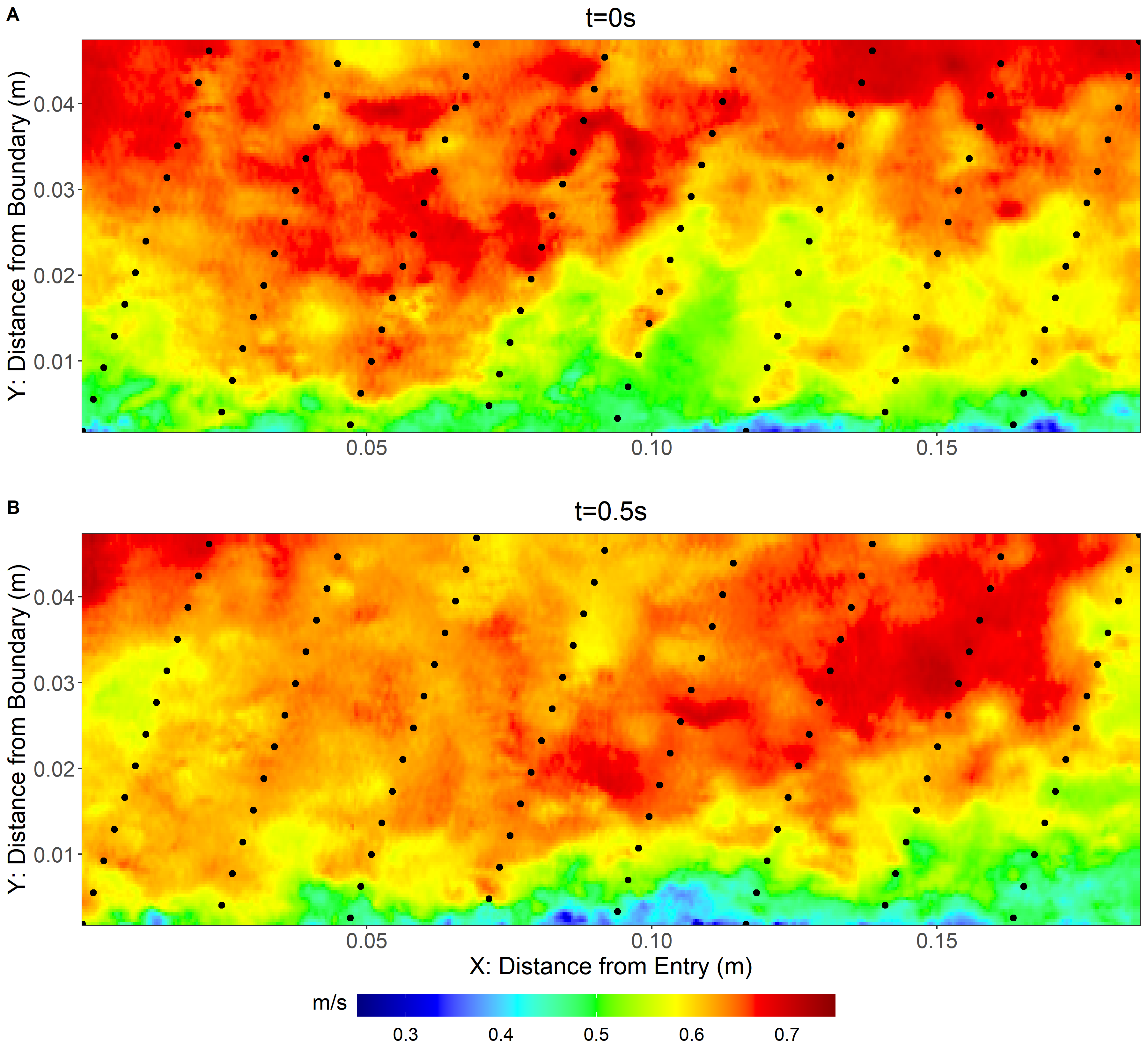
Figure 1: Wind speed in m/s for the wind-field data from Kat et al. (2017) at the initial time (panel A) and at $t=0.5$s (panel B). The black dots represent the 100 subsampled locations used for analysis and forecasting.

3 Methodology

We introduce a DESN in Section 3.1 and the DLSM in Section 3.2. In Section 3.3 we propose the physics-informed, double-reservoir model used throughout this work. We also present the physics-informed inference in Section 3.4. The forecast calibration and uncertainty quantification are deferred to the supplementary material.

3.1 Deep Echo-State Networks

DESNs (see, e.g., McDermott and Wikle (2017, 2019a, 2019b)) are stochastic modifications of a recurrent NN assuming that the weights connecting the input to the hidden states and the weights interconnecting the hidden states to themselves are drawn from some prior distribution controlled by some parameters. The introduction of stochastic weight matrix avoids any inherent instabilities associated with gradient based optimization algorithms (i.e., backpropagation) of recurrent NNs. Additionally, instead of estimating any weight as a parameter, the ESN implies that a small parametric space can be optimized using a cross-validation approach, thereby reducing the computational cost.

A DESN is formulated as follows (McDermott and Wikle, 2019b):

output: $$\qquad\mathbf{Y}_{t}=\mathbf{B}_{D}\mathbf{h}_{t,D}+\sum_{d=1}^{D-1}\mathbf{B}_{d}k\left(\tilde{\mathbf{h}}_{t,d}\right)+\boldsymbol{\epsilon}_{t},$$ (1a)

hidden state $$d \qquad\mathbf{h}_{t,d}=(1-\alpha)\mathbf{h}_{t-1,d}+\alpha\boldsymbol{\omega}_{t,d},$$: (1b)

$$\qquad\boldsymbol{\omega}_{t,d}=f_{h}\left(\frac{\zeta_{d}}{|\lambda_{W_{d}}|}\mathbf{W}_{d}\mathbf{h}_{t-1,d}+\mathbf{W}_{d}^{\text{in}}\tilde{\mathbf{h}}_{t,d-1}\right),\text{ for }d>1,$$ (1c)

reduction $$d-1 \qquad\tilde{\mathbf{h}}_{t,d-1}\equiv Q\left(\mathbf{h}_{t,d-1}\right),\text{ for }d>1,$$: (1d)

input: $$\qquad\boldsymbol{\omega}_{t,1}=f_{h}\left(\frac{\zeta_{1}}{|\lambda_{W_{1}}|}\mathbf{W}_{1}\mathbf{h}_{t-1,1}+\mathbf{W}_{1}^{\text{in}}\mathbf{x}_{t}\right),$$ (1e)

matrix distribution: $$\qquad W_{d_{i,j}}=\gamma^{W_{d}}_{i,j}p(\eta_{W_{d}})+(1-\gamma^{W_{d}}_{i,j})\delta_{0},$$ (1f)

$$\qquad W^{\text{in}}_{d_{i,j}}=\gamma^{W_{d}^{\text{in}}}_{i,j}p(\eta_{W_{d}^{\text{in}}})+(1-\gamma^{W_{d}^{\text{in}}}_{i,j})\delta_{0},$$ (1g)

$$\qquad\gamma^{W_{d}}_{i,j}\text{\;$\thicksim$\;}Bern(\pi_{W_{d}}),\quad\gamma^{W_{d}^{\text{in}}}_{i,j}\text{\;$\thicksim$\;}Bern(\pi_{W_{d}^{\text{in}}}).$$

Here, $d=\{1,\dots,D\}$ represents the depth or the number of layers in the network. The output $\mathbf{Y}_{t}$ is expressed as a linear combination $\mathbf{B}_{D}\mathbf{h}_{t,D}+\sum_{d=1}^{D-1}\mathbf{B}_{d}k_{h}\left(\tilde{\mathbf{h}}_{t,d}\right)+\boldsymbol{\epsilon}_{t}$ in (1a), while $\mathbf{h}_{t,D}$ is an $n_{h,D}$-dimensional state vector, $\tilde{\mathbf{h}}_{t,d}$ is an $n_{\tilde{h},d}$-dimensional state vector, and $\mathbf{B}_{d}$ are matrices with unknown entries. The error term $\boldsymbol{\epsilon}_{t}$ in (1a) is assumed to be independent identically distributed in time and is denoted as a multivariate normal distribution with zero mean. The dimension of the hidden state $\mathbf{h}_{t,d}$ is reduced using the function $Q(\cdot)$ in equation (1d). This results in the $n_{\tilde{h},d}$-dimensional hidden state $\tilde{\mathbf{h}}_{t,d}$, and in this work, we use an empirical orthogonal function approach as a dimension reduction function $Q(\cdot)$. The $k(\cdot)$ in equation (1a) represents some scaling function needed to ensure that the values of $\tilde{\mathbf{h}}_{t,d}$ are on a similar scale to those within $\mathbf{h}_{t,D}$ (i.e., the range of values which the two vectors take is similar or the same). In equations (1c) and (1e), the term $\boldsymbol{\omega}_{t,d}$ is derived from a nonlinear function (activation function) $f_{h}$ with some pre-specified forms such as the hyperbolic tangent or rectified linear unit (Goodfellow et al., 2016). This function combines the past hidden state $\mathbf{h}_{t-1,d}$ and some layer specific input data. This input data is specified as either the $n_{x}$-dimensional vector of input $\mathbf{x}_{t}$, which comprises of the past/lagged values of $\mathbf{Y}_{t}$, (i.e., $\mathbf{x}_{t}=\left(\mathbf{Y}_{t-\tau},\ldots,\mathbf{Y}_{t-m\tau}\right)^{\top}$, where $\tau$ represents the forecast lead time (McDermott and Wikle, 2017)) and $m\geq 1$ represents the total number of lags of the lead-time to retain, or the dimension reduced hidden state from the prior layer $\tilde{\mathbf{h}}_{t,d-1}$. A spike-and-slab prior is used to inform the entries of the weight matrices $\mathbf{W}_{d}$ and $\mathbf{W}^{\text{in}}_{d}$ in (1f) and (1g) where individual entries of these matrices take a value of zero with some given probability $\pi_{W_{d}}$ and $\pi_{W_{d}^{\text{in}}}$ for $\mathbf{W}_{d}$ and $\mathbf{W}^{\text{in}}_{d}$, respectively. The non-zero elements of the weight matrices are drawn from some symmetric distribution centered about zero (Lukosevicius, 2012) and for this work we assume $p(\cdot)\sim Unif(-1,1)$, however other choices of distribution have been shown to be effective choices in previous works (see McDermott and Wikle (2017); Huang et al. (2021); Bonas and Castruccio (2023); Yoo and Wikle (2023)). Lastly, the DESN must also respect the echo-state property, i.e. after a sufficiently long time sequence, the model must asymptotically lose its dependence on the initial conditions (Lukosevicius, 2012; Jaeger, 2007). This property holds when the spectral radius (largest eigenvalue) of $\mathbf{W}_{d}$, denoted by $\lambda_{W_{d}}$, is less than one. The scaling parameter $\zeta_{d}\in(0,1]$ is introduced to ensure that the spectral radius does not violate this condition on equation (1c) and (1e). Following McDermott and Wikle (2019b), we fix the hyper-parameters $\pi_{W_{d}}$ and $\pi_{W_{d}^{\text{in}}}$ to 0.1, as the results have been shown to be robust with respect to this choice. We assume that $n_{h,d}=n_{h}$ and $n_{\tilde{h},d}=n_{\tilde{h}}$, and we denote the model hyper-parameters by $\boldsymbol{\theta}_{ESN}=\{n_{h},n_{\tilde{h}},m,\{\zeta_{d},d=1,\ldots,D\},\lambda_{r},\alpha,D\}$, thereby excluding $\mathbf{B}_{d},d=1,\ldots,D$, which are estimated separately as will be discussed in Section 3.4.

3.2 Deep Liquid State Machines

Traditional machine learning models such as feedforward NNs compute and transmit continuous valued signals throughout the network. Unlike these, spiking NNs rely on discrete spike streams (binary sequences) to process information, and were formulated to more closely mimic natural biological NNs (Maass, 1997). In this work, we formulate a dynamic version of a spiking NN, a DLSM (Maass et al., 2002), which discretizes the input through a leaky integrate-and-fire model (LIF, Burkitt (2006); Zhang et al. (2018)), which we detail in Section 3.2.1. In Section 3.2.2 we provide the mathematical description of the DLSM. The notation in Section 3.2.1 will be used exclusively for introducing the LIF model, whereas in Section 3.2.2 a slightly different notation will be used, in order to align it with the DESN in the previous Section.

3.2.1 Preliminaries: The Leaky Integrate-and-Fire Model

The LIF models the dynamics of $\mathbf{s}_{t}=\{{s}^{(i)}_{t};i=1,\dots,n_{h}\}$, a $n_{h}$-dimensional binary discrete time series whose input is another $(m+1)$-dimensional binary discrete time series $\mathbf{I}_{t}=\{I^{(j)}_{t};j=1,\dots,m+1\}$. Heuristically, the said input impacts the membrane potential energy $\boldsymbol{V}_{\text{mem}}(t)=\{{V}^{(i)}_{\text{mem}}(t);i=1,\dots,n_{h}\}$, and once it crosses a threshold $V_{\text{thr}}$ (which in this work is the same for each neuron $i$) it allows the output to be one, i.e., $s^{(i)}_{t}=1$. Once the threshold is passed, the potential is set to a resting value $V_{\text{res}}$, which we fix to zero for all $i$. Finally, during each time step, a small portion of the membrane potential energy is ‘leaked’ out, and the overall potential membrane energy is decreased by a value $V_{\text{leak}}$, again identical for each $i$.

Formally, for each neuron $i$ the LIF model is defined as follows:

$${V_{\text{mem}}^{(i)}(t)}=\sum_{j\in\Phi}w_{j;i}I_{t}^{(j)}-V_{\text{leak}}+V^{(i)}_{\text{mem}}(t-1),\quad\text{if}\quad V^{(i)}_{\text{mem}}(t)<V_{\text{thr}},$$ (2a)

$$V^{(i)}_{\text{mem}}(t)=V_{\text{res}},\quad\text{if}\quad V^{(i)}_{\text{mem}}(t)\geq V_{\text{thr}},$$ (2b)

$$s^{(i)}_{t}=\left\{\begin{array}[]{lr}1,&\text{if }V^{(i)}_{\text{mem}}(t)\geq V_{\text{thr}},\\ 0,&\text{if }V^{(i)}_{\text{mem}}(t)<V_{\text{thr}},\end{array}\right.$$ (2e)

where $\Phi$ represents the set of synapses for which the input impacts the membrane potential, $w_{j;i}$ are the synapse weights for neuron $i$ associated with the input spike stream $I_{t}^{(j)}$ which is either 1 or 0. The membrane potential is updated using equation (2a), compared against the threshold in equation (2b) and possibly reset to the resting state. The individual elements of the output are defined in equation (2e).

3.2.2 Mathematical Definition of Liquid State Machines

A DLSM is a reservoir computing model based on the same principle of random sparse matrices as the DESN in equations (1c) and (1e), adapted to the case of spiking NNs. Here, for each time point $t$ we assume a dynamic model on a sub-time scale $t^{*}=1,\ldots,T^{*}$, and we count the number of output spikes generated by a LIF model. More formally, we redefine $\boldsymbol{\omega}_{t,d}$ from equations (1c) and (1e) as the total number of spikes from the LIF model in Section 3.2.1:

$$\boldsymbol{\omega}_{t,d}=\sum_{t^{*}=1}^{T^{*}}\mathbf{s}_{t^{*},d},$$

where $\boldsymbol{\omega}_{t,d}$ is a vector of size $n_{h}$ as in the DESN model in equation (1). We further specify the evolution of the vector of the neurons’ potential energy $\boldsymbol{V}_{\text{mem}}(t^{*})$ during each sub-time point, $t^{*}$ by reformulating equations (1c) and (1e) as follows:

$$\Delta\boldsymbol{V}_{\text{mem}}(t^{*})=\frac{\zeta}{|\lambda_{W}|}\mathbf{W}\mathbf{s}_{t^{*}-1}+\mathbf{W}^{\text{in}}\tilde{\mathbf{x}}_{t^{*}}-V_{\text{leak}}-\text{max}(\mathbf{s}_{t^{*}})V_{\text{inhib}},$$ (3a)

$$\Delta\boldsymbol{V}_{\text{mem}}(t^{*})=0\quad\text{if}\quad\mathbf{s}_{t^{*}-\tilde{t}}=1,\quad\forall\tilde{t}\in[0,V_{\text{latent}}],$$ (3b)

Here, $\tilde{\mathbf{x}}_{t^{*}}$ represents the input spike stream, $\boldsymbol{I}_{t^{*}}=(I^{(j)}_{t^{*}};j=1,\ldots,n_{x})$, from equation (2). We allow the neurons to go through a latency period $V_{\text{latent}}$ after emitting a spike to emulate the natural delayed response from the stimulus of the spike (Levakova et al., 2015). This latency period forces the neurons’ membrane potential energy to neither increase nor decay over a fixed number of sub-time points. We also allow each neuron to exhibit lateral inhibition (Cohen, 2011), or the ability of neurons to reduce the membrane potential energy of the other neurons in the same layer when they emit a spike. Lateral inhibition is implemented by reducing the membrane potential energy of every neuron in the hidden state by some fixed amount, $V_{\text{inhib}}$, when one neuron emits a spike. The total number of hyper-parameters for the DLSM are then $\boldsymbol{\theta}=\{\boldsymbol{\theta}_{ESN},V_{\text{thr}},V_{\text{leak}},V_{\text{inhib}},V_{\text{latent}}\}$, where $\boldsymbol{\theta}_{ESN}$ is the same hyper-parameter vector as in the DESN.

In order to feed data into the DLSM, the continuous input we use in our application must be converted into spike trains. To convert the input data, $\mathbf{x}_{t}$ for the first layer and $\tilde{\mathbf{h}}_{t,d}$ for all subsequent layers, from equations (1c) and (1e) into spike trains, the data must first be rescaled using min-max normalization, formally:

$$\mathbf{x}_{t}^{\prime}=\frac{\mathbf{x}_{t}-\text{min}(\mathbf{x}_{t})}{\text{max}(\mathbf{x}_{t})-\text{min}(\mathbf{x}_{t})}.$$

The $n_{x}$-length vector $\mathbf{x}_{t}^{\prime}$ is then converted to a matrix of spike trains, $\tilde{\mathbf{x}}_{t^{*}}$, of dimension $n_{x}\times T^{*}$, by creating spike trains of length $T^{*}$ with firing rates proportional to the scaled vector elements of $\mathbf{x}_{t}^{\prime}$. This approach resembles spike train conversion in image classification, where the gray levels and color intensities of a pixel are converted into spike trains with firing rates proportional to their pixel value (Wijesinghe et al., 2019), hence implying that the values are drawn from a Poisson process (O’Connor et al., 2013; Cao et al., 2014; Diehl et al., 2015). The use of a sub-time scale $T^{*}$ implies a considerable increase in the length of the observational vector. For example in our work we choose $T^{*}=100$, and the conversion into spike trains converts a network with $n=1,000$ observations to one with $n\times T^{*}=100,000$ observations. The specification of $T^{*}$ is solely dictated by the computational resources available, as a small value would allow faster computation but lower accuracy of the spike train in representing the signal, while a larger value than the one proposed would make the computation practically impossible.

3.3 Deep Double-Reservoir Network

In this work, we combine a DESN and a DLSM in a deep double reservoir network (DDRN) to improve the flexibility and the predictability of the underlying process. Formally, the DDRN reformulates the output of the model in equation (1a) as:

$$\qquad\mathbf{Y}_{t}=\mathbf{Z}^{\text{(DESN)}}_{t}+\mathbf{Z}^{\text{(DLSM)}}_{t}+\boldsymbol{\epsilon}_{t},$$ (4a)

$$\qquad\mathbf{Z}^{\text{(DESN)}}_{t}=\mathbf{B}^{\text{(DESN)}}_{D}\mathbf{h}^{\text{(DESN)}}_{t,D}+\sum_{d=1}^{D-1}\mathbf{B}^{\text{(DESN)}}_{d}k\left(\tilde{\mathbf{h}}^{\text{(DESN)}}_{t,d}\right),$$ (4b)

$$\qquad\mathbf{Z}^{\text{(DLSM)}}_{t}=\mathbf{B}^{\text{(DLSM)}}_{D}\mathbf{h}^{\text{(DLSM)}}_{t,D}+\sum_{d=1}^{D-1}\mathbf{B}^{\text{(DLSM)}}_{d}k\left(\tilde{\mathbf{h}}^{\text{(DLSM)}}_{t,d}\right),$$ (4c)

which assumes a linear combination of the hidden states (reservoirs) from the DESN and DLSM to explain the output $\mathbf{Y}_{t}$. The model coefficients $\mathbf{B}=\{\mathbf{B}_{d}^{\text{(DESN)}},\mathbf{B}_{d}^{\text{(DLSM)}},d=1,\ldots,D\}$ are unknown and need to be estimated as detailed in the next Section.

3.4 Inference with Physics-Based Networks

A portion of the observed training data is held out for validation and used to perform inference for the hyper-parameter vector $\boldsymbol{\theta}$. For a fixed $\boldsymbol{\theta}$ the set of parameters comprising of the collection of all matrices $\mathbf{B}$ from equation (4) is estimated according to the method described in this Section. The predictions are then produced and the resulting mean squared error (MSE) is minimized with respect to the set of hyper-parameters in $\boldsymbol{\theta}$.

The simplest approach to estimate the coefficients in $\mathbf{B}$ is via a matrix version of ridge regression with some penalty $\lambda_{r}$ (see the supplementary material for a detailed description), which is computationally affordable and prevents exceedingly large estimator variance by adding some bias (McDermott and Wikle, 2017; Huang et al., 2021; Bonas and Castruccio, 2023; Yoo and Wikle, 2023). In this work, we operate under the assumption that additional context is available about the underlying spatio-temporal process in the form of a PDE, and it is of interest to integrate it in the analysis by penalizing the inference towards it. Indeed, beyond producing accurate point forecasts with our proposed model, we are also interested in ensuring that the forecast at least loosely follows the physical laws characterizing the underlying spatio-temporal process. To ensure this, instead of using an $L^{2}$ penalty as in the case of ridge regression, the loss function is modified to include a penalty quantifying the extent of the departure of the estimated process to the physical equation. Formally, if we denote by $Y_{t}(\mathbf{s})$ the time varying continuous field of interest, we assume we are given a spatio-temporal PDE in the form of (Raissi et al., 2019):

$$\frac{\partial{Y}_{t}(\mathbf{s})}{\partial t}+N[Y_{t}(\mathbf{s})]=0,$$

where $N[Y_{t}(\mathbf{s})]$ is a (possibly nonlinear) differential operator, which in this work is assumed to be known. For example, in the case of the viscous Burgers’ equation in Section 4.1, the process is one dimensional in space so that $\mathbf{s}=x$ and the operator is defined as $N[Y_{t}(x)]=\xi_{1}Y_{t}(x)\frac{\partial Y_{t}(x)}{\partial x}-\xi_{2}\frac{\partial^{2}Y_{t}(x)}{\partial x^{2}}$, with $\xi_{1}$ and $\xi_{2}$ assumed to be known.

Instead of enforcing this equation strictly, we only penalize the departure of the solution from the equation. Formally, for the estimated process $\hat{Y}_{t}(\mathbf{s})$, we define

$$\hat{g}_{t}(\mathbf{s})=\frac{\partial\hat{Y}_{t}(\mathbf{s})}{\partial t}+N[\hat{Y}_{t}(\mathbf{s})]$$

so that in the case of a perfect physics-obeying solution we have $\hat{g}_{t}(\mathbf{s})=0$ for all $\mathbf{s}$ and $t$. We then construct a new penalty which trades off the prediction skills with the magnitude of the aforementioned quantify (Raissi et al., 2019):

$$\text{MSE}_{\text{pred}+\text{phys}}=(1-\chi)\text{MSE}_{\text{pred}}+\chi\text{MSE}_{\text{phys}},$$ (5)

$$\text{MSE}_{\text{pred}}=\frac{1}{NT}\sum_{i=1}^{N}\sum_{t=1}^{T}|{Y}_{t}(\mathbf{s}_{i})-\hat{{Y}}_{t}(\mathbf{s}_{i})|^{2},$$

$$\text{MSE}_{\text{phys}}=\frac{1}{NT}\sum_{i=1}^{N}\sum_{t=1}^{T}|\hat{{g}}_{t}(\mathbf{s}_{i})|^{2},$$

where $\text{MSE}_{\text{pred}}$ is the MSE for the point forecasts to the true process $Y_{t}(\mathbf{s})$ and $\text{MSE}_{\text{phys}}$ corresponds to the error respective to the PDE. The parameter $\chi\in[0,1]$ represents the relative weight of the predictive MSE with respect to the physical constraints, which we consider as an additional hyper-parameter. We denote this model as Physics Informed DDRN (PIDDRN). Unlike the ridge regression case, there is no closed-form for either the solution nor the gradient of $\text{MSE}_{\text{pred}+\text{phys}}$. As such, given the very large number of parameters with respect to which the optimization is sought, we provide an initial estimate from ridge regression and minimize only a fraction of total number of parameters. Indeed, we introduce one additional hyper-parameter, $\psi\in[0,1]$, which represents a proportion of the output parameters, $\mathbf{B}$, to be optimized via this approach, while the remaining $\lfloor(1-\psi)|\mathbf{B}|\rfloor$ parameters are fixed. This additional hyper-parameter ensures that the PIDDRN model will perform at least as well as the DESN and DDRN models and it also considerably decreases the computational time. The results from PIDDRN compared to the previous models will be shown in Sections 4 and 5.

4 Simulation Study

We aim to assess the predictive capabilities of the PIDDRN model against the non physics-informed DDRN, the DESN, as well as other time series and machine learning approaches. In this section, we focus on simulated data from the viscous Burgers’ equation (Burgers, 1948), which we introduce in Section 4.1. We show a comparison in terms of their predictive ability and uncertainty quantification in Section 4.2.

Reservoir computing methods such as DESN have been shown to produce computationally affordable forecasts owing to the use of random sparse matrices (McDermott and Wikle, 2017; Huang et al., 2021; Bonas and Castruccio, 2023; Yoo and Wikle, 2023), and the PIDDRN is no exception. Even with the addition of the DLSM and the physics-informed loss function, inference can still be achieved in a reasonable time. For this simulation study, we were able to produce 1000 ensemble forecasts using the PIDDRN in parallel using only 24 cores at 2.50Ghz frequency in less than 8 hours. This approach could easily be up-scaled by increasing the number of cores.

4.1 Viscous Burgers’ Equation

The viscous Burgers’ equation is often employed as a simple surrogate for the Navier-Stokes equations. Here we take the one-dimensional form which describes the space-time velocity of a fluid of a given constant viscosity $\nu>0$ (Bateman, 1915; Burgers, 1948). Formally, it is defined as:

$$\frac{\partial Y_{t}(x)}{\partial t}+Y_{t}(x)\frac{\partial Y_{t}(x)}{\partial x}=\nu\frac{\partial^{2}Y_{t}(x)}{\partial x^{2}}$$ (6)

where $Y_{t}(x)$ is the fluid velocity at some location $x$ and time point $t$. We simulate data at $N=30$ uniformly distributed spatial locations on $x\in[-1,1]$ across 500 time steps. We solve the equation using a spatial discretization of 1/15 and temporal discretization of 3/1000 (so a total time of 1.5), a choice which allows for a numerically stable solution to the PDE. We specify two different initial conditions: a sinusoid $Y_{0}(x)=-\sin(\pi x)$ and a Gaussian curve $Y_{0}(x)=e^{-x^{2}}$. Additionally, we consider viscosity values of $\nu=\left\{10^{-s};s=1,\dots,4\right\}$, for a total of 8 different simulation setups. The simulated data with $Y_{0}(x)=-\sin(\pi x)$ and $\nu=0.01$ can be seen in Figure 2A, as well as the velocity $Y_{t}(x)$ for all $x$ at times $t=0$, $t=100$, and $t=500$ in Figure 2B. Each model was trained for each of the simulations using the first $T=450$ time steps and was tested using the next $\tau=50$ steps. We produced forecasts using 1000 ensembles, each representing an independent draw for the weight matrices $\mathbf{W}_{d}$ and $\mathbf{W}^{\text{in}}_{d}$ in equations (1f), (1g) and (3). The grids used with the validation approach to optimize the hyper-parameter space are shown in the supplementary material in Table S1. In Section S.2.1 of the supplementary material we further show the ability of the proposed PIDDRN model to produce accurate long lead forecasts on a generalized Burgers’ equation with an external forcing (Büyükaşık and Pashaev, 2013).

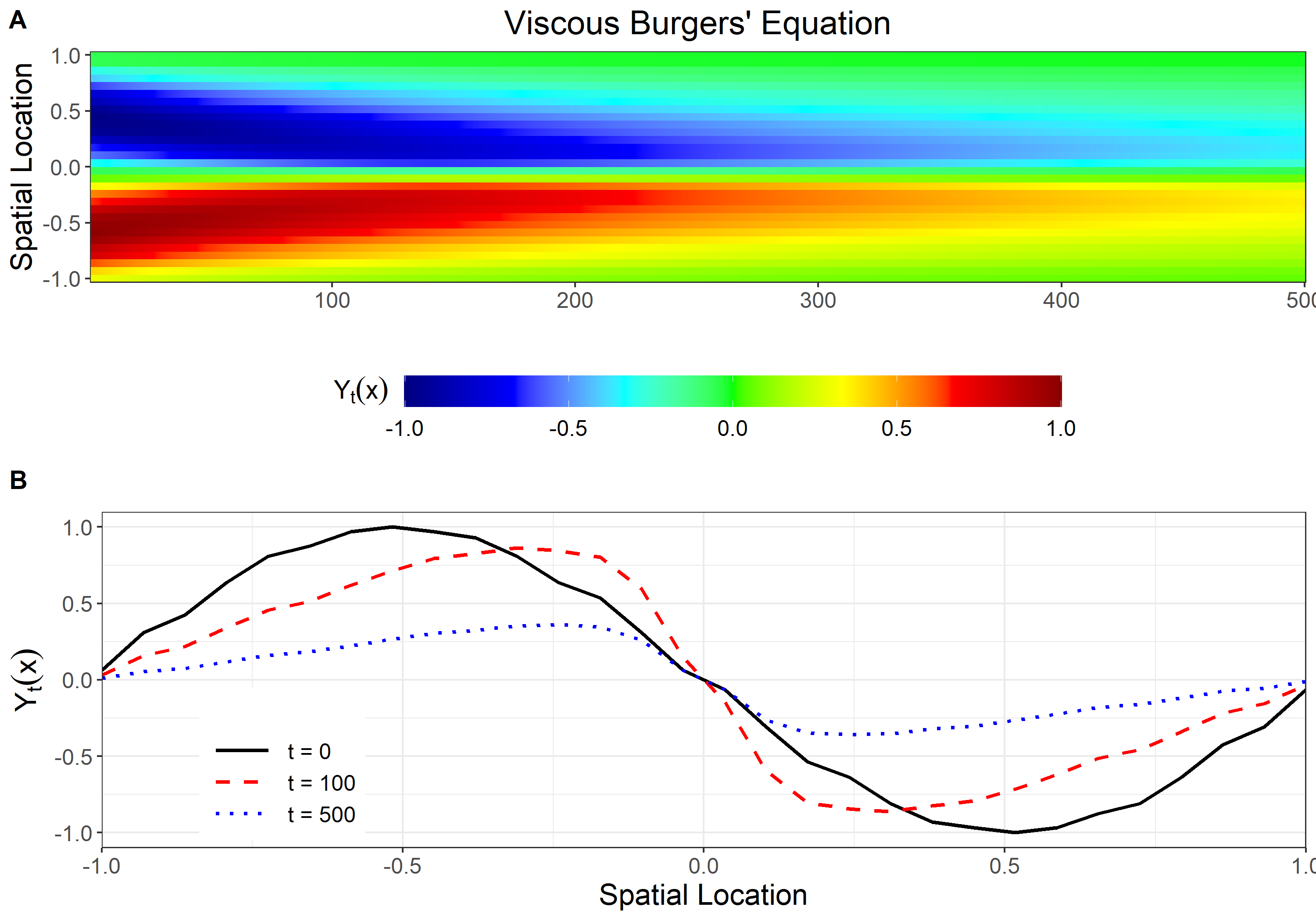
Figure 2: Solution of the viscous Burgers’ equation from equation (6) with initial condition $Y_{0}(x)=-\sin(\pi x)$ and viscosity $\nu=0.01$. (A) Heatmap across all points in time ($x$ axis) and space ($y$ axis). (B) Solution for spatial points, for three time points $t=0$, $t=100$ and $t=500$.

4.2 Point Forecasts and Uncertainty Quantification

We compare the forecasting performance of PIDDRN not only with the DDRN and DESN models described above, but also with other time series and machine learning approaches. We choose an auto-regressive, fractionally integrated moving average model (ARFIMA, Granger and Joyeux (1980); Hosking (1981)) as well as a standard machine learning approach for time series, the long short-term memory model (LSTM, Hochreiter and Schmidhuber (1997)). This model is a special case of a recurrent NN, but relies on fully connected, dense weight matrices which are optimized via gradient-based methods (technical details are provided in the supplementary material).

The forecasting skills are assessed using DESN as a reference model, and the relative performance of every aforementioned model is computed with respect to MSE${}_{\text{pred}+\text{phys}}$ in equation (5). The results are shown in Table 1, with the average performance across all viscosity values and the standard deviation in parenthesis. It can easily be seen how the PIDDRN dramatically outperforms all other models. More specifically, the PIDDRN model returns an average improvement of MSE${}_{\text{pred}+\text{phys}}$ for the sinusoidal initial condition of 54.05% (with standard deviation $24.69\%$) and for the Gaussian initial condition of 49.72% ($24.83\%$). The PIDDRN also shows a dramatically improved prediction against ARFIMA and LSTM, whose negative values indicate worse performance than the reference DESN for both initial conditions. Additionally, the PIDDRN model outperforms its non-physics-informed counterpart, the DDRN, which has a smaller improvement over the standard DESN of 21.82% (16.87%) and 45.67% (17.67%) for the two initial conditions.

Forecasting Method	$Y_{0}(x)=-\text{sin}(\pi x)$	$Y_{0}(x)=e^{-x^{2}}$
PIDDRN	54.05 (24.69)	49.72 (24.83)
DDRN	21.82 (16.87)	45.67 (17.67)
DESN	—	—
ARFIMA	-311.50 (376.82)	-84.25 (56.66)
Long Short-Term Memory	-20.14 (69.47)	-10.23 (42.77)

Table 1: Percent improvement of forecasting performance for each model versus the DESN in terms of the MSE${}_{\text{pred}+\text{phys}}$ metric described in equation (5). An average across all simulated datasets is shown with the standard deviation in parenthesis.

To further illustrate the improvement of the PIDDRN model, the spatio-temporal maps of MSE${}_{\text{pred}+\text{phys}}$ for the non-physics-informed DESN and physics-informed PIDDRN model for the initial condition $Y_{0}(x)=-\text{sin}(\pi x)$ with viscosity $\nu=0.01$ can be seen in Figure 3(A-B). It can be seen how the non-physics-informed DESN produce almost uniformly (in space and time) worse results than PIDDRN. The relative ordering of improvement among the models from Table 1 is clearly demonstrated in this figure, where it is shown how the target prediction metric progressively improves, with PIDDRN being able to effectively capture the spatio-temporal areas which have forecasting inadequacies in DESN.

The Burgers’ equation assumes a one dimensional fluid excited by an initial condition, progressively decaying through the action of the viscosity and hence gradually losing energy. In order to assess the physical consistency of PIDDRN forecasts against DESN, in Figure 3(C) we compare the total energy of the system, calculated as the squared integral in space for each time point, as a function of forecast lead time (as anomalies from the last observed time point). It can be seen how the PIDDRN model correctly predicts a monotonically decreasing energy, while DESN, being not informed about the physical properties of the equation, produces an unphysical energy increase, especially at large lead times.

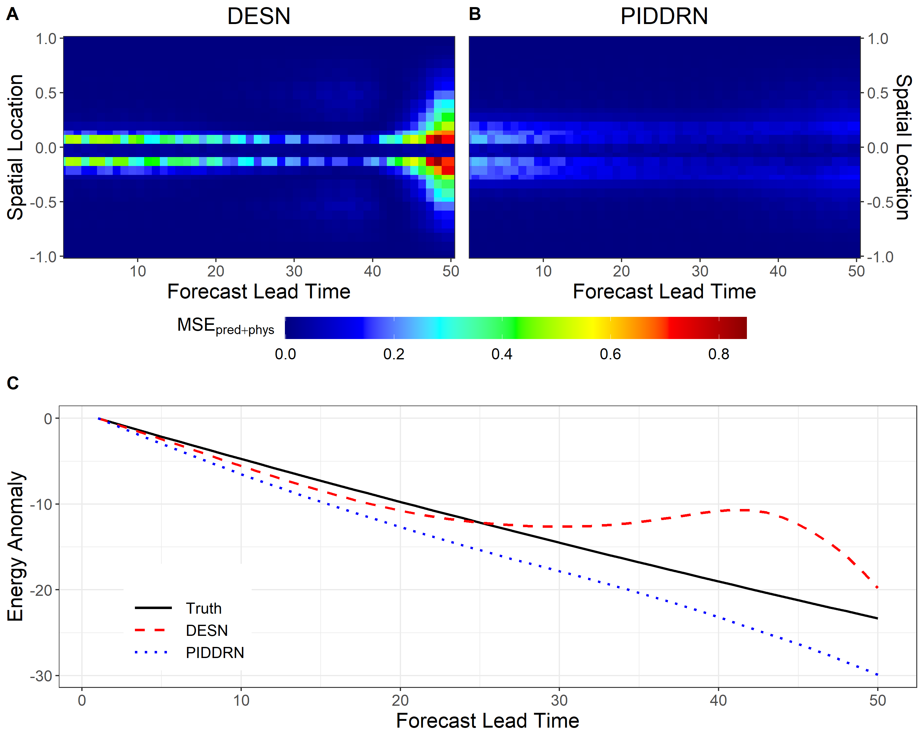
Figure 3: Prediction comparison in terms of the MSE${}_{\text{pred}+\text{phys}}$ from (5) for the viscous Burgers’ equation (6). The first row (panels A and B) represents data from the simulation where $Y_{0}(x)=-\text{sin}(\pi x)$ and $\nu=0.01$. The second row panels (C) represents the total energy profile (in terms of energy anomaly with respect to the initial forecast time point) of the system across space through time, for both the DESN and PIDDRN models.

The calibration method discussed in the supplementary material was implemented to produce uncertainty estimates surrounding the PIDDRN forecasts. Table 2 shows a comparison of the marginal uncertainty quantification when the forecasts are uncalibrated (i.e., using the estimates of the standard deviations from the ensemble of forecasts, McDermott and Wikle (2017)) and calibrated using the aforementioned approach. This table shows that, when using the uncalibrated estimates, the marginal uncertainty is incorrectly quantified, thereby resulting in a drastically smaller coverage of the nominal 95%, 90%, and 80% prediction intervals (PIs). Indeed, the average discrepancy in coverage from the uncalibrated estimates across all simulations is 11.7% across the three intervals. When using the uncertainty estimates produced by the calibration approach, the marginal uncertainty is more correctly quantified and does capture an appropriate amount of the true data within the specified intervals. In fact, the calibrated 95% PI now captures an average of 92.5% of the true data across both space and time for all simulations and only produce a coverage discrepancy of 1.9% across the three intervals.

Prediction Interval	Uncalibrated	Calibrated
95%	82.6 (12.7)	92.5 (3.3)
90%	77.0 (17.0)	89.7 (3.3)
80%	70.3 (21.0)	82.9 (2.6)

Table 2: Uncertainty quantification methods compared in terms of their nominal 95% PI coverage on data from the Burgers’ equation (6). The ensemble-based (uncalibrated) approach is outlined in McDermott and Wikle (2017) and the quantile regression (calibrated) approach is the method detailed in Bonas et al. (2023). The mean coverage across all simulations for both initial conditions as well as the standard deviation (in parenthesis) is reported.

5 Application

We now apply our proposed PIDDRN model to forecast the boundary layer velocity for the application presented in Section 2. The first $T=490$ time steps were used for training whereas the remaining $\tau=10$ points were used as the testing data, and we produced forecasts for 1000 ensembles. The final 10 points in the training data were used as the validation set to optimize the hyper-parameters for the models, and the grid search is identical to that used for the Burgers’ equation in Section 4. We use the following hyper-parameters for the reservoir computing models: $D=2$, $n_{h}=150$, $n_{\tilde{h}}=30$, $\lambda_{r}=10^{-1}$, $\zeta=\{0.4,0.8\}$, $m=1$, $\pi_{W}=0.1,\pi_{W^{\text{in}}}=0.1$, $p(\cdot)\sim Unif(-1,1)$ , $\alpha=0.66$, $T^{*}=100$, $V_{\text{thr}}=2.5$, $V_{\text{res}}=0$, $V_{\text{leak}}=0.9$, $V_{\text{inhib}}=1.0$, $V_{\text{latent}}=0$, $\psi=0.05$. We also assume $\chi=0.5$ in equation (5), i.e., the predictive error and the physical constraints are equally weighted. The derivation of the PDE penalty from the incompressible Navier Stokes equations is relatively involved so for the sake of simplicity it is deferred to the supplementary material, thus we only report the final result. In our application the velocity $Y_{t}(\mathbf{s})$ reduces to a scalar component in the $x$ direction as a function of $x$ and $y$, so that $\mathbf{s}=(x,y)$. While the model and the forecasts are spatio-temporal, the forecasts are averaged in time and denoted as $\bar{Y}=\bar{Y}(x,y)$, and the PDE penalty is expressed with respect to this quantity:

$$\frac{u_{\tau}^{2}}{\delta}~{}+\frac{u_{\tau}\delta}{\text{Re}_{\tau}}\frac{\partial^{2}\bar{Y}}{\partial y^{2}}+\left\{(\kappa y)^{2}\left|\frac{\partial\bar{Y}}{\partial y}\right|\right\}\frac{\partial\bar{Y}}{\partial y}~{}=0,$$ (7)

.

where $\kappa$ is defined in the supplementary material and $\delta,u_{\tau},\text{Re}_{\tau}$ are parameters defined in Section 2. The PDE in (7) will be used to define the function $\hat{g}$ in (5) (which here is only a spatial function) and the target function to minimize.

We show a comparison of each of the models in terms of predictive ability in Section 5.1 and in terms of uncertainty quantification in Section 5.2.

5.1 Point Forecasts

We will show the forecasting performance of the PIDDRN model in terms of the physics-based loss against the other similar reservoir computing models, the time series approach ARFIMA, and the machine learning approach LSTM, in terms of the time average of the forecast $\bar{u}$. Similar to Table 1, Table 3 shows the relative improvement in terms of the forecasts on the test data using the newly defined loss function against the standard DESN model. As it is shown, this table illustrates how the PIDDRN again outperforms each of the other methods presented. In fact, the PIDDRN model produces a 10.09% improvement over the DESN for this application, a result further illustrated in Figure 4. Additionally, the PIDDRN model has a more significant improvement over the next best models, the LSTM and DDRN models, where they only produce an improvement of 5.31% and 0.79%, respectively. Finally, the time series reference model ARFIMA is the only model in this instance to produce deteriorating results in terms of the MSE, for it produces results which are 10.48% worse than that of the DESN.

The spatio-temporal maps of the forecasting MSE${}_{\text{pred}+\text{phys}}$ for the entire domain for the DESN and PIDDRN models can be seen in Figure 4(A-B). The forecasts from the 100 locations were used to interpolate the entire spatio-temporal domain using thin plate splines (Green and Silverman, 1994) and then these interpolated forecasts are used to calculate the MSE${}_{\text{pred}+\text{phys}}$ across the entire space. Figure 4 shows the loss functions. Since we rely on a time-averaged simplification of the Navier-Stokes equations, the said loss is also time-independent. From these panels it can be seen how the PIDDRN produces remarkably better forecasting performance versus the DESN based models, a result consistent with those presented in Table 3. The DESN model fails to produce entirely accurate forecasts for the spatial domain in terms of the point prediction and physical constraints.

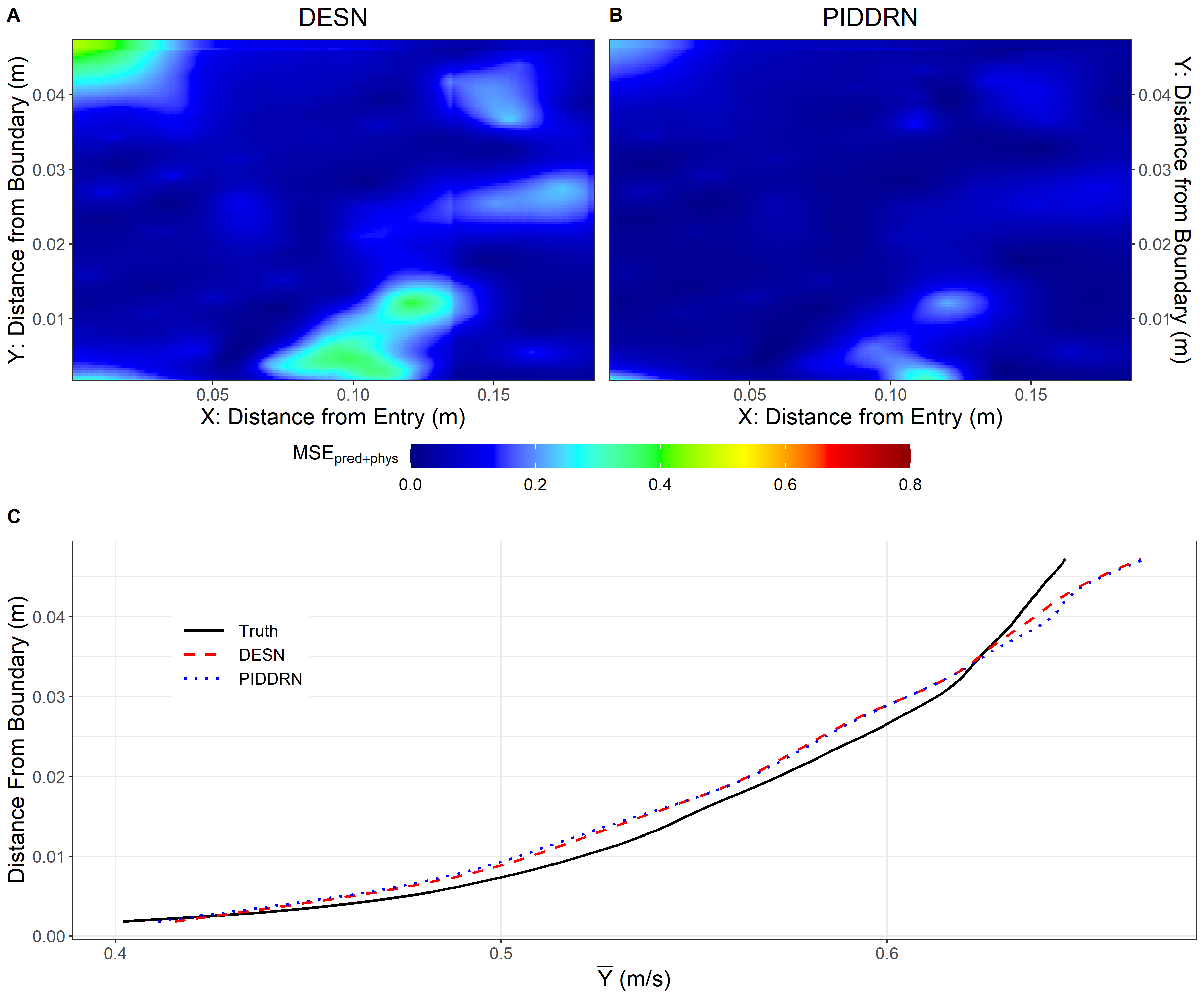
Figure 4: A comparison of the MSE${}_{\text{pred}+\text{phys}}$ from equation (5) across the entire space time domain of the time -averaged Wind-field data for the DESN (panel A) and PIDDRN (panel B) models. Panel C shows the estimated vertical profiles for the forecasts from both the DESN and PIDDRN models, averaged both in time and across $x$.

We also compare the PIDDRN forecasts against the DESN and the data through the estimated vertical profile in panel C of Figure 4. In this case, both models estimate the true time- and $x$-averaged profile well, however a case could be made that the PIDDRN predictions are more physically consistent. Indeed, in our application and according to our derivation in the supplementary material the velocity divergence reduces to $\frac{\partial\bar{Y}}{\partial x}=0$, so that mass conservation can be estimated by the extent to which this term is close to 0. Under this metric the PIDDRN model drastically outperforms the other models, for this term returns an average value of 1.45 (with spatial standard deviation of 21.9) whereas the DESN and DDRN models return values of 1.72 (21.2) and 1.78 (21.8), respectively.

To further show the physical consistency of the PIDDRN forecasts versus the DESN, we can also compute the variance of the fluctuation component $u^{{}^{\prime}}_{t}$ in time, for each of the forecasts produced from their respective models. Given that we are penalizing the time-averaged velocity $\bar{u}$, we expect these variances to more closely follow those produced from the data, despite the penalization not being directly applied to the instantaneous velocity $u_{t}$. Thus we can simply calculate the MSE between the true fluctuation variances and the forecast fluctuations. In this instance, we observe that the DESN model produces an average MSE in time (with standard deviation in parenthesis) of 0.01 (0.003) whereas the PIDDRN model returns a value of 0.007 (0.002). This further details how the PIDDRN produces more physically appropriate and consistent forecasts that the DESN model.

Forecasting Method	Relative Improvement
PIDDRN	10.09
DDRN	0.79
DESN	—
ARFIMA	-10.48
Long Short-Term Memory	5.31

Table 3: Percent improvement of forecasting performance for each model versus the DESN in terms of the MSE${}_{\text{pred}+\text{phys}}$ metric described in equation (5) for the Wind-field application data.

5.2 Uncertainty Quantification

As was the case with the simulated data in Section 4, the calibration method discussed in the supplementary material was implemented with the PIDDRN model to produce uncertainty estimates surrounding the forecasts. In this instance we chose $n_{w}=20$ as part of the implementation. Table 4 shows a comparison of the marginal uncertainty quantification when the forecasts are uncalibrated and calibrated using the aforementioned approach. From this table it can be seen that, when using the uncalibrated estimates, the marginal uncertainty is incorrectly quantified which leads to a worse coverage of the nominal 95%, 90%, and 80% prediction intervals (PIs). Here the average discrepancy in coverage from the uncalibrated estimates across all of the 100 subsampled location is 9.3% across the three intervals. When using the uncertainty estimates produced by the calibration approach it is clearly seen from the table how the marginal uncertainty is now correctly quantified and does capture an appropriate amount of the true data within the specified intervals. More specifically, the calibrated 95% PI now capture an average of 93.0% of the true data across both space and time for all locations. When using the calibrated intervals, there is only a coverage discrepancy of 2.4% across the three intervals, thus further exemplifying the improvement over the uncalibrated approach.

Prediction Interval	Uncalibrated	Calibrated
95%	99.1 (4.5)	93.0 (11.1)
90%	98.4 (5.6)	90.1 (14.8)
80%	95.4 (10.5)	84.1 (18.4)

Table 4: Uncertainty quantification methods compared in terms of their nominal 95% PI coverage on Wind-field data. The ensemble-based (uncalibrated) approach is outlined in McDermott and Wikle (2017) and the quantile regression (calibrated) approach is the method detailed in Bonas et al. (2023). The mean across the 100 subsampled locations is reported with the standard deviation in parenthesis.

6 Conclusion

In this work we have introduced a new approach to forecasting boundary layer velocity by combining two reservoir computing approaches while also incorporating a physical constraints with a PDE penalization. The proposed model is able to achieve superior forecasting skills while (partly) complying with physical constraints, as well as accurate uncertainty quantification. While the proposed approach has been applied to a turbulent flow in a controlled experimental setting, the principles underpinning the proposed methodology are applicable to any spatio-temporal data set for which additional context in the form of a PDE (or systems of PDEs) is available.

Our proposed approach comprises of two main innovations. Firstly, we combine two deep reservoir computing methods, Echo State Networks and Liquid State Machines, one relying on continuous signals, the other one on spike trains. Secondly, inference is not performed with a standard bias-variance tradeoff approach such as ridge regression, but with a physics-informed penalty stemming from a PDE, which is assumed to be known and at least partially descriptive of the underlying process dynamics. The resulting physics-informed deep double reservoir model significantly outperforms the other reference models presented, such as ARIMA and LSTMs, in terms of their forecasting skills in both the case of the simulated Burgers’ equations (Burgers, 1948) data in Section 4 as well as the application detailed in Section 2 with corresponding results in Section 5. Crucially, the forecast is also more compliant with some key physical properties such as energy dissipation (for the simulation study) as well as mass conservation and realism of the fluctuating velocity signal (for the application). In order to calibrate the uncertainty propagated by the two reservoir computing approaches, we further augment the ensemble predictions with the calibration approach and showed how this results in accurate uncertainty quantification.

The proposed method is based on on combining two reservoir computing approaches, whose flexibility stems from the ability to capture nonlinear dynamics without requiring very large training data as standard recurrent NNs. More importantly from a statistics perspective, this work contributes to a model-based view of this class of methods, which have been originally envisioned as a possible solution to the vanishing/exploring gradient when performing inference on a recurrent NNs. While reservoir computing models do indeed sidestep the issue of the numerical instabilities in gradient calculation via cross-validation on a small parameter space, from a statistician perspective this is only the consequence on the use of prior in the weight matrices. As such, while the introduction of additional uncertainty is necessary, our stance is that such uncertainty can and should be quantified in the same fashion as any other statistical model.

The addition of a physical constrain in the model via optimization of a modified, PDE-driven penalty represent a powerful, simple and appealing unifying framework for problems ranging from data-rich/context-poor to data-poor/context-rich. It does, however, come with associated issues one should be aware of. Since the penalization is adding a bias in the inference towards what is believed to be a more physically consistent process, the physics-based forecast is bound to have inferior short-term point-predictive skills (measured as MSE). In this work, we have shown that this loss of predictability is counter-balanced with some degree of preservation of additional physical properties in the forecast, such as loss of energy and mass conservation, as well as improved long lead forecasting in the simulation study. Clearly, which properties are to preserved is a very application dependent question and contextualization of the problem is necessary.

While the proposed approach has shown improved forecasting skills in turbulent layer wind in a controlled laboratory, this represents only the first step towards an operational use on a real case scenarios such as turbulent three-dimensional boundary layer winds induced by wake effects in wind turbines and/or complex terrain. In these types of cases, many if not all the simplifying assumptions of the Navier-Stokes equation which allowed us to reduce the problem to a scalar PDE will have to be relaxed. As such, a real-case penalty will need to be a system of PDEs more akin to the original equations, possibly coupled with those associated to the pressure field, with a considerable increase in the computational overhead. What will be the simplifying assumptions on the PDE penalty that will allow the inference to still be computationally feasible is expected to be a challenging future area of research.

Supplementary Material

We provide the R code to apply the DESN, DDRN, and PIDDRN forecasting approaches mentioned in Sections 3 on a simulated Burgers’ equation (Burgers, 1948) data with 30 spatial locations and 500 time steps. This code and data can be found in the following GitHub repository: github.com/MBonasND/2023PIDDRN.

References

- Ak et al. (2016) Ak, R., O. Fink, and E. Zio (2016). Two machine learning approaches for short-term wind speed time-series prediction. IEEE Transactions on Neural Networks and Learning Systems 27(8), 1734–1747.
- Bateman (1915) Bateman, H. (1915). Some recent researches on the motion of fluids. Monthly Weather Review 43(4), 163–170.
- Baydin et al. (2018) Baydin, A. G., B. A. Pearlmutter, A. A. Radul, and J. M. Siskind (2018). Automatic differentiation in machine learning: a survey. Journal of Marchine Learning Research 18, 1–43.
- Bonas and Castruccio (2023) Bonas, M. and S. Castruccio (2023). Calibration of spatial forecasts from citizen science urban air pollution data with sparse recurrent neural networks. Annals of Applied Statistics 17(3), 1820–1840.
- Bonas et al. (2023) Bonas, M., C. K. Wikle, and S. Castruccio (2023). Calibrated forecasts of quasi-periodic climate processes with deep echo state networks and penalized quantile regression. arXiv:2308.04391.
- Burgers (1948) Burgers, J. (1948). A mathematical model illustrating the theory of turbulence. Volume 1 of Advances in Applied Mechanics, pp. 171–199. Elsevier.
- Burkitt (2006) Burkitt, A. (2006). A review of the integrate-and-fire neuron model: I. homogeneous synaptic input. Biological Cybernetics 95, 1–19.
- Büyükaşık and Pashaev (2013) Büyükaşık, S. A. and O. K. Pashaev (2013). Exact solutions of forced burgers equations with time variable coefficients. Communications in Nonlinear Science and Numerical Simulation 18(7), 1635–1651.
- Cao et al. (2014) Cao, Y., Y. Chen, and D. Khosla (2014). Spiking deep convolutional neural networks for energy-efficient object recognition. International Journal of Computer Vision 113(1), 54–66.
- Clifton et al. (2014) Clifton, A., M. H. Daniels, and M. Lehning (2014). Effect of winds in a mountain pass on turbine performance. Wind Energy 17(10), 1543–1562.
- Cohen (2011) Cohen, R. A. (2011). Lateral Inhibition, pp. 1436–1437. New York, NY: Springer New York.
- Conry et al. (2015) Conry, P., A. Sharma, M. J. Potosnak, L. S. Leo, E. Bensman, J. J. Hellmann, and H. J. S. Fernando (2015). Chicago’s heat island and climate change: Bridging the scales via dynamical downscaling. Journal of Applied Meteorology and Climatology 54(7), 1430 – 1448.
- Demolli et al. (2019) Demolli, H., A. S. Dokuz, A. Ecemis, and M. Gokcek (2019). Wind power forecasting based on daily wind speed data using machine learning algorithms. Energy Conversion and Management 198, 111823.
- Diehl et al. (2015) Diehl, P. U., D. Neil, J. Binas, M. Cook, S.-C. Liu, and M. Pfeiffer (2015). Fast-classifying, high-accuracy spiking deep networks through weight and threshold balancing. 2015 International Joint Conference on Neural Networks (IJCNN).
- Fernando and Weil (2010) Fernando, H. J. S. and J. C. Weil (2010). Whither the stable boundary layer?: A shift in the research agenda. Bulletin of the American Meteorological Society 91(11), 1475 – 1484.
- Fernando et al. (2010) Fernando, H. J. S., D. Zajic, S. Di Sabatino, R. Dimitrova, B. Hedquist, and A. Dallman (2010, 05). Flow, turbulence, and pollutant dispersion in urban atmospheresa). Physics of Fluids 22(5), 051301.
- Goodfellow et al. (2016) Goodfellow, I., Y. Bengio, and A. Courville (2016). Deep Learning. MIT Press. http://www.deeplearningbook.org.
- Granger and Joyeux (1980) Granger, C. W. J. and R. Joyeux (1980). An introduction to long-memory time series models and fractional differencing. Journal of Time Series Analysis 1(1), 15–29.
- Green and Silverman (1994) Green, P. and B. Silverman (1994). Nonparametric regression and generalized linear models: a roughness penalty approach. United Kingdom: Chapman and Hall.
- Hochreiter and Schmidhuber (1997) Hochreiter, S. and J. Schmidhuber (1997, 11). Long Short-Term Memory. Neural Computation 9(8), 1735–1780.
- Hosking (1981) Hosking, J. R. M. (1981). Fractional differencing. Biometrika 68(1), 165–176.
- Huang et al. (2021) Huang, H., S. Castruccio, and M. G. Genton (2021). Forecasting high-frequency spatio-temporal wind power with dimensionally reduced echo state networks. Journal of the Royal Statistical Society - Series C 71(2), 449–466.
- Huang and Chalabi (1995) Huang, Z. and Z. Chalabi (1995). Use of time-series analysis to model and forecast wind speed. Journal of Wind Engineering and Industrial Aerodynamics 56(2), 311–322.
- Jaeger (2001) Jaeger, H. (2001). The “echo state” approach to analysing and training recurrent neural networks-with an erratum note. Bonn, Germany: German National Research Center for Information Technology GMD Technical Report 148.
- Jaeger (2007) Jaeger, H. (2007). Echo state network. Scholarpedia 2(9), 2330.
- Kat et al. (2017) Kat, R. D., L. Gan, D. Fiscaletti, J. Dawson, and B. Ganapathisubramani (2017, December). Wide-field time-resolved particle image velocimetry data of a turbulent boundary layer. https://eprints.soton.ac.uk/416120/.
- Khosravi et al. (2018) Khosravi, A., L. Machado, and R. Nunes (2018). Time-series prediction of wind speed using machine learning algorithms: A case study Osorio wind farm, Brazil. Applied Energy 224, 550–566.
- Larsen et al. (2022) Larsen, A., I. Hanigan, B. Reich, Y. Qin, M. Cope, G. Morgan, and A. Rappold (2022). A deep learning approach to identify smoke plumes in satellite imagery in near-real time for health risk communication. Journal of Exposure Science & Environmental Epidemiology 31(170-176).
- Lei et al. (2009) Lei, M., L. Shiyan, J. Chuanwen, L. Hongling, and Z. Yan (2009). A review on the forecasting of wind speed and generated power. Renewable and Sustainable Energy Reviews 13(4), 915–920.
- Levakova et al. (2015) Levakova, M., M. Tamborrino, S. Ditlevsen, and P. Lansky (2015). A review of the methods for neuronal response latency estimation. Biosystems 136, 23–34.
- Lukosevicius (2012) Lukosevicius, M. (2012). A practical guide to applying echo state networks. In Neural Networks: Tricks of the Trade, pp. 659–686. Springer.
- Maass (1997) Maass, W. (1997). Networks of spiking neurons: The third generation of neural network models. Neural Networks 10(9), 1659–1671.
- Maass et al. (2002) Maass, W., T. Natschläger, and H. Markram (2002). Real-Time Computing Without Stable States: A New Framework for Neural Computation Based on Perturbations. Neural Computation 14(11), 2531–2560.
- Mateńczuk and et. al. (2021) Mateńczuk, K. and et. al. (2021). Financial time series forecasting: Comparison of traditional and spiking neural networks. Procedia Computer Science 192, 5023–5029. Knowledge-Based and Intelligent Information & Engineering Systems: Proceedings of the 25th International Conference KES2021.
- McDermott and Wikle (2017) McDermott, P. L. and C. K. Wikle (2017). An ensemble quadratic echo state network for non-linear spatio-temporal forecasting. Stat 6(1), 315–330.
- McDermott and Wikle (2019a) McDermott, P. L. and C. K. Wikle (2019a). Bayesian recurrent neural network models for forecasting and quantifying uncertainty in spatial-temporal data. Entropy 21(2), 184.
- McDermott and Wikle (2019b) McDermott, P. L. and C. K. Wikle (2019b). Deep echo state networks with uncertainty quantification for spatio‐temporal forecasting. Environmetrics 30(3), e2553.
- Meng et al. (2020) Meng, X., Z. Li, D. Zhang, and G. E. Karniadakis (2020). Ppinn: Parareal physics-informed neural network for time-dependent pdes. Computer Methods in Applied Mechanics and Engineering 370, 113250.
- North et al. (2022) North, J. S., C. K. Wikle, and E. M. Schliep (2022). A bayesian approach for spatio-temporal data-driven dynamic equation discovery. arXiv:2209.02750.
- O’Connor et al. (2013) O’Connor, P., D. Neil, S.-C. Liu, T. Delbruck, and M. Pfeiffer (2013). Real-time classification and sensor fusion with a spiking deep belief network. Frontiers in Neuroscience 7, 178.
- Pang et al. (2020) Pang, G., M. D’Elia, M. Parks, and G. Karniadakis (2020). npinns: Nonlocal physics-informed neural networks for a parametrized nonlocal universal laplacian operator. algorithms and applications. Journal of Computational Physics 422, 109760.
- Raissi et al. (2019) Raissi, M., P. Perdikaris, and G. Karniadakis (2019). Physics-informed neural networks: A deep learning framework for solving forward and inverse problems involving nonlinear partial differential equations. Journal of Computational Physics 378, 686–707.
- Rosselló et al. (2016) Rosselló, J. L., M. L. Alomar, A. Morro, A. Oliver, and V. Canals (2016). High-density liquid-state machine circuitry for time-series forecasting. International Journal of Neural Systems 26(05), 1550036.
- Sangalli (2021) Sangalli, L. M. (2021). Spatial regression with partial differential equation regularisation. International Statistical Review 89(3), 505–531.
- Sangalli et al. (2013) Sangalli, L. M., J. O. Ramsay, and T. O. Ramsay (2013). Spatial spline regression models. Journal of the Royal Statistical Society: Series B (Statistical Methodology) 75(4), 681–703.
- Stull (1988) Stull, R. B. (1988). An Introduction to Boundary Layer Meteorology. Kluwer Academic Publishers: Dordrecht.
- Wei et al. (2021) Wei, D., J. Wang, X. Niu, and Z. Li (2021). Wind speed forecasting system based on gated recurrent units and convolutional spiking neural networks. Applied Energy 292, 116842.
- Wijesinghe et al. (2019) Wijesinghe, P., G. Srinivasan, P. Panda, and K. Roy (2019). Analysis of liquid ensembles for enhancing the performance and accuracy of liquid state machines. Frontiers in Neuroscience 13, 504.
- Yoo and Wikle (2023) Yoo, M. and C. K. Wikle (2023). Using echo state networks to inform physical models for fire front propagation. Spatial Statistics 54, 100732.
- Zhang et al. (2018) Zhang, A., W. Zhu, and J. Li (2018, 12). Spiking echo state convolutional neural network for robust time series classification. IEEE Access 7, 4927–4935.
- Zhang et al. (2019) Zhang, D., L. Lu, L. Guo, and G. E. Karniadakis (2019). Quantifying total uncertainty in physics-informed neural networks for solving forward and inverse stochastic problems. Journal of Computational Physics 397, 108850.