Pharmacokinetic/Pharmacodynamic Anesthesia Model
Incorporating psi-Caputo Fractional Derivatives

Abstract

We present a novel Pharmacokinetic/Pharmacodynamic (PK/PD) model for the induction phase of anesthesia, incorporating the $\psi$-Caputo fractional derivative. By employing the Picard iterative process, we derive a solution for a nonhomogeneous $\psi$-Caputo fractional system to characterize the dynamical behavior of the drugs distribution within a patient’s body during the anesthesia process. To explore the dynamics of the fractional anesthesia model, we perform numerical analysis on solutions involving various functions of $\psi$ and fractional orders. All numerical simulations are conducted using the MATLAB computing environment. Our results suggest that the $\psi$ functions and the fractional order of differentiation have an important role in the modeling of individual-specific characteristics, taking into account the complex interplay between drug concentration and its effect on the human body. This innovative model serves to advance the understanding of personalized drug responses during anesthesia, paving the way for more precise and tailored approaches to anesthetic drug administration.

Keywords: Pharmacokinetic/Pharmacodynamic model; fractional calculus; $\psi$-Caputo fractional derivative; numerical simulations.

MSC 2020: 34A08, 92C45.

1 Introduction

Pharmacokinetic/Pharmacodynamic (PK/PD) modeling is a mathematical approach used in pharmacology to study the relationship between drug concentrations (Pharmacokinetics) and their effects on the body (Pharmacodynamics) [31, 37]. The PK/PD models help researchers and clinicians to understand how drugs are absorbed, distributed, metabolized, and eliminated from the body [7].

The PK/PD models integrate Pharmacokinetic and Pharmacodynamic data to characterize the time course of drug action [29] . These models can be simple or complex, depending on the drug’s characteristics and the purpose of the modeling. The parameters of these models were fitted by Schnider et al. in [36]. Some common types of PK/PD models include:

1. Linear PK/PD models. The basic structure of a linear PK/PD model consists of two main components: the Pharmacokinetic component, which describes the drug concentration-time profile in the body, and the Pharmacodynamic component, which relates to the drug concentration to the observed effect [16].

2. Non-linear PK/PD models. These models can incorporate various components, such as saturable drug elimination, receptor binding kinetics, and indirect response models. These models provide a more accurate representation of the concentration-effect relationship and can be used to optimize dosing regimens and predict drug responses in different populations [11].

3. Mechanistic PK/PD models. These models incorporate known biological mechanisms, such as drug-receptor interactions, enzyme kinetics, or signal transduction pathways. They provide a more detailed representation of drug action but require more data and knowledge about the underlying biology [33].

4. Population Pharmacokinetic models. These models are used to describe the time course of drug exposure in patients and to investigate sources of variability in patient exposure. They can be used to simulate alternative dose regimens, allowing for informed assessment of dose regimens before study conduct [10, 32].

In recent years, the field of fractional derivatives has emerged as a promising approach to model and understand complex biological processes characterized by non-integer order dynamics [21, 27, 35]. This unique mathematical framework has found diverse applications in various areas of biology, where traditional integer-order calculus falls short in capturing the intricacies of these systems [6, 25].

One prominent field where fractional derivatives have made significant contributions is Neurobiology. By employing fractional calculus, researchers have been able to delve into the dynamics of neural systems with a greater level of realism. This includes modeling the behavior of neurons, synaptic transmission, and the propagation of nerve impulses. The incorporation of fractional derivatives enables the consideration of memory effects and non-local behavior, providing a more accurate representation of neural processes [28].

Another area where fractional derivatives have shown their efficacy is in Biomedical Signal Processing. Biomedical signals, such as electroencephalograms (EEG), electrocardiograms (ECG), and blood pressure signals, are often complex and exhibit non-integer order dynamics. By utilizing fractional order filters and operators, meaningful information can be extracted from these signals, leading to improved analysis and interpretation. Fractional calculus has proven to be a valuable tool in enhancing our understanding of these vital physiological signals [15].

Furthermore, the field of Cancer Modeling has witnessed the application of fractional derivatives [34]. Tumor growth and the intricate interactions between cancer cells and the immune system present complex dynamics that can be effectively captured using fractional order models. By incorporating non-local effects and memory into the modeling process, fractional derivatives provide a comprehensive framework for studying cancer progression. This approach has the potential to shed light on the underlying mechanisms and aid the development of novel therapeutic strategies [2, 39].

The field of Pharmacokinetics and Pharmacodynamics plays a crucial role in understanding the behavior of drugs in biological systems [37]. Traditional PK/PD models have predominantly relied on integer-order derivatives to describe various processes involved in drug absorption, distribution, metabolism, and elimination [13, 31, 43]. However, these models often fall short in accurately capturing the complexity of Pharmacokinetic behaviors [8, 19].

Fractional calculus offers a promising alternative by providing a more precise representation of these intricate dynamics [38]. A number of studies have shown that certain drugs follow an anomalous kinetics that can hardly be represented by classical models. Indeed, fractional-order pharmacokinetics models have proved to be better suited to represent the time course of these drugs in the body and also they can describe memory effects and a power-law terminal phase. Therefore, they give rise to more complex kinetics that better reflects the complexity of the human body. In [19], a fractional one-compartment model with a continuous intravenous infusion is considered, where it allows to determine how the infusion rate influences the total amount of drug in the compartment. Moreover, in the case of multiple dosing administration, recurrence relations for the doses and the dosing times that also prevent drug accumulation are presented. Hence, in [9], a PK model was introduced employing a fractional-order approach akin to mammillary dynamics. This model was specifically designed to incorporate considerations of tissue entrapment, thereby altering the anticipated drug concentration profiles. The proposed model shows a limitation in data fit profiles, without transgressing the fundamental principles of mass balance and physiological states. The mathematical study of the amount of drug administered as a continuous intravenous infusion or oral dose for fractional-order mammillary type models is investigated in [30].

For pharmacokinetic and pharmacodynamic models, the first fractional one was introduced in [40]. By utilizing the Caputo fractional derivative, the authors presented a fresh perspective on the intricate relationships between drug dosages, absorption rates, and therapeutic outcomes. Since then, some few applications of fractional PK/PD models have appeared in the literature [3, 20]. In [3], the authors study the discrete and discrete fractional representation of a PK/PD model describing tumor growth and anti-cancer effects in continuous time considering a specific times scale, while in [20] a fractional PK/PD model in anesthesia is developed to describe the nonlinear characteristics of the PK/PD patient models.

In this article, we propose a novel fractional four-compartmental PK/PD model for the induction phase of anesthesia, employing the $\psi$-Caputo fractional derivative. This innovative approach involves replacing each ordinary derivative in the classical PK/PD model investigated in [41, 43] with the $\psi$-Caputo fractional derivative of order $\alpha\in(0,1]$ [1].

By incorporating fractional derivatives into the model, we aim to capture the intricate dynamics of anesthesia induction more accurately. Furthermore, based on the Picard iterative process, we establish a solution for the nonhomogeneous $\psi$-Caputo fractional differential system of equations in terms of matrix Mittag-Leffler functions. The solution provides a deeper understanding of the dynamics and behavior of the anesthesia process, taking into account the complex interplay between drug concentration and its effect on the body.

To validate the effectiveness of our proposed model, we conduct numerical simulations. Specifically, we determine the optimal anesthesia dosage for a 53-year-old male weighing 77 Kg and measuring 177 cm, while considering the minimum treatment time [41]. These simulations enable us to evaluate the performance and applicability of the fractional PK/PD model in a practical context.

Through the article, we aim to demonstrate the potential of fractional derivatives in advancing our understanding of biology, particularly in the field of PK/PD modeling. By incorporating fractional calculus into these models, we can unlock new insights and improve our ability to predict and optimize drug behavior within biological systems.

The paper is organized as follows. In Section 2, we provide a review of several definitions and properties of fractional calculus that are essential for our subsequent discussions (Section 2.1); and we recall the Pharmacokinetic and Pharmacodynamic models proposed by Bailey et al. [5] and Schnider [36] (Section 2.2), discussing their bispectral index (Section 2.3) and the equilibrium points (Section 2.4). Our original contributions are then given in Section 3: we obtain a solution to a general linear nonhomogeneous $\psi$-Caputo fractional system (Section 3.1); we introduce a novel PK/PD model for the induction phase of anesthesia based on the $\psi$-Caputo fractional derivative (Section 3.2); and finally we compute the model parameters using the Schnider model [36], presenting the numerical results of the fractional PK/PD model corresponding to different $\psi$ functions and fractional orders (Section 3.3). We conclude with Section 4, discussing the implications and limitations of our results, and with Section 5, summarizing our findings and outlining potential directions for future research.

2 Preliminaries

In this section, we recall several definitions, properties of fractional calculus, and the classical PK/PD model, that will be used in the sequel.

2.1 Fundamental definitions and results

Throughout the paper, $\psi$ designates a function of class $C^{1}[a,b]$ such that $\psi^{\prime}(t)>0$, for all $t\in[a,b]$.

Definition 1 (See [26]).

The left $\psi$-Riemann-Liouville fractional integral of a function $f$ of order $\alpha\in(0,1)$ is defined by

$$I_{a}^{\alpha,\psi}f(t)=\dfrac{1}{\Gamma(\alpha)}\int_{a}^{t}\psi^{\prime}(s)\left(\psi(t)-\psi(s)\right)^{\alpha-1}f(s)\,\mathrm{d}s,$$

where $\Gamma(\cdot)$ is the Euler Gamma function.

Remark 1.

We remark that $\Gamma(x+1)=x\Gamma(x)$, for all $x>0$, and for any positive integer $n$ we have $\Gamma(n+1)=n!$.

Definition 2 (See [26]).

The $\psi$-Caputo fractional derivative of a function $f$ of order $\alpha\in(0,1)$ can be defined as follows:

$${}^{C}\!D_{a}^{\alpha,\psi}f(t)=\dfrac{1}{\Gamma(1-\alpha)}\int_{a}^{t}\left(\psi(t)-\psi(a)\right)^{-\alpha}f^{\prime}(s)\,\mathrm{d}s.$$

We have the following properties of the fractional operators with respect to function $\psi$.

Lemma 1 (See [26]).

Let $\Re(\alpha)>0$ and $\Re(\beta)>0$. Then,

$$I_{a}^{\alpha,\psi}\left(f(x)-f(a)\right)^{\beta-1}(t)=\dfrac{\Gamma(\beta)}{\Gamma(\beta+\alpha)}\left(f(t)-f(a)\right)^{\beta-\alpha-1}.$$

Theorem 1 (See [1]).

Let $\alpha\in(0,1)$ and $f\in C^{1}(a,b)$. Then,

$$I_{a}^{\alpha,\psi}{}^{C}\!D_{a}^{\alpha,\psi}f(t)=f(t)-f(a).$$

The Mittag–Leffler function appears naturally in the solution of fractional differential equations and in its various applications: see [17, 24] and references therein.

Definition 3 (See [17]).

The Mittag–Leffler function of one parameter, of a matrix $A$, is defined as

$$E_{\alpha}(A)=\sum_{l=0}^{+\infty}\frac{A^{l}}{\Gamma(\alpha l+1)},\quad Re(\alpha)>0.$$ (1)

Definition 4 (See [17]).

The Mittag–Leffler function of two parameters, of a matrix $A$, is defined as

$$E_{\alpha,\alpha^{\prime}}(A)=\sum_{l=0}^{+\infty}\frac{A^{l}}{\Gamma(\alpha l+\alpha^{\prime})},\quad Re(\alpha)>0,~{}\alpha^{\prime}>0.$$ (2)

Remark 2.

The matrix exponential function is a special case of the matrix Mittag–Leffler function [24]. For $\alpha^{\prime}=1$, we have $E_{\alpha,1}(A)=E_{\alpha}(A)$ and $E_{1,1}(A)=e^{A}$.

We now recall the notion of generalized convolution integral.

Definition 5 (See [23]).

Let $f$ and $g$ be two functions which are piecewise continuous at any interval $[a,b]$ and of exponential order. The generalized convolution of $f$ and $g$ is defined by

$$\left(f\ast_{\psi}g\right)(t)=\int_{a}^{t}f(s)g\left(\psi^{-1}(\psi(t)+\psi(a)-\psi(s))\right)\psi^{\prime}(s)\,\mathrm{d}s.$$

2.2 The classical PK/PD model: state of the art

The Pharmacokinetic/Pharmacodynamic (PK/PD) model comprises four compartments: intramuscular blood $(y_{1}(t))$, muscle $(y_{2}(t))$, fat $(y_{3}(t))$, and the effect site $(y_{4}(t))$. The inclusion of the effect site compartment (representing the brain) is necessary to account for the finite equilibration time between the central compartment and the central nervous system concentrations [5]. This model is employed to characterize the distribution of drugs within a patient’s body and can be mathematically described by a four-dimensional dynamical system:

$$\left\{\begin{array}[]{l l}\dot{y}_{1}(t)=-(a_{1\,0}+a_{1\,2}+a_{1\,3})\,y_{1}(t)+a_{2\,1}\,y_{2}(t)+a_{3\,1}\,y_{3}(t)+u(t),\\ \dot{y}_{2}(t)=a_{1\,2}\,y_{1}(t)-a_{2\,1}\,y_{2}(t),\\ \dot{y}_{3}(t)=a_{1\,3}\,y_{1}(t)-a_{3\,1}\,y_{3}(t),\\ \dot{y}_{4}(t)=\frac{a_{e\,0}}{v_{1}}\,y_{1}(t)-a_{e\,0}\,y_{4}(t),\end{array}\right.$$ (3)

subject to the initial conditions

$$y_{1}(0)=y_{2}(0)=y_{3}(0)=y_{4}(0)=0,$$ (4)

where $y_{1}(t)$, $y_{2}(t)$, $y_{3}(t)$ and $y_{4}(t)$ represent, respectively, the masses of the propofol in the compartments of blood, muscle, fat, and effect site at time $t$. The control $u(t)$ represents the continuous infusion rate of the anesthetic. The parameters $a_{1\,0}$ and $a_{e\,0}$ represent, respectively, the rate of clearance from the central compartment and the effect site. The parameters $a_{1\,2}$, $a_{1\,3}$, $a_{2\,1}$, $a_{3\,1}$ and $a_{e\,0}/v_{1}$ are the transfer rates of the drug between compartments. All these parameters depend on age, weight, height and gender, and the relations can be found in Table 1.

A schematic diagram of the dynamical control system (3) is given in Figure 1.

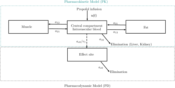
Figure 1: Schematic diagram of the PK/PD model with the effect site compartment of Bailey and Haddad [5].

Table 1: Parameter values for model (3) according with Schnider models [36].

Parameter	Estimation
$a_{10}\,(min^{-1})$	$0.443+0.0107\,(\text{weight}-77)-0.0159\,(\text{LBM}-59)+0.0062\,(\text{height}-177)$
$a_{12}\,(min^{-1})$	$0.302-0.0056\,(\text{age}-53)$
$a_{13}\,(min^{-1})$	0.196
$a_{21}\,(min^{-1})$	$\left(1.29-0.024\,(\text{age}-53)\right)/\left(18.9-0.391\,(\text{age}-53)\right)$
$a_{31}\,(min^{-1})$	0.0035
$a_{e0}\,(min^{-1})$	0.456
$v_{1}\,(l)$	4.27

Following Schnider et al. [36], the lean body mass (LBM) is calculated using the James formula, which performs satisfactorily in normal and moderately obese patients, but not so well for severely obese cases [22]. The James formula calculates LBM as follows:

$$\text{for Male},\,\text{LBM} = 1.1\times\text{weight}-128\times\left(\dfrac{\text{weight}}{\text{height}}\right)^{2},$$ (5)

$$\text{for Female},\,\text{LBM} = 1.07\times\text{weight}-148\times\left(\dfrac{\text{weight}}{\text{height}}\right)^{2}.$$ (6)

2.3 The bispectral index (BIS)

The bispectral index (BIS) serves as an indicator of anesthesia depth, obtained by analyzing the electroencephalogram (EEG) signal and reflecting the effect site concentration of $y_{4}(t)$. It provides a quantitative measure of a patient’s level of consciousness, ranging from 0 (indicating no cerebral activity) to 100 (representing a fully awake patient). According to clinical guidelines, maintaining BIS values within the range of 40 to 60 is considered essential to ensure adequate general anesthesia during surgical procedures [4]. BIS values below 40 indicate a deep hypnotic state, while values above 60 may increase the risk of awareness under anesthesia. Thus, it is crucial to closely monitor and regulate the BIS value within the optimal range of 40 to 60 to prevent unintended consciousness during anesthesia and ensure patient safety [14].

Empirically, the BIS can be described by a decreasing sigmoid function, as outlined by Bailey et al. [5]:

$$BIS(y_{4}(t))=BIS_{0}\left(1-\dfrac{y_{4}(t)^{\gamma}}{y_{4}(t)^{\gamma}+EC_{50}^{\gamma}}\right),$$ (7)

where the parameters in the BIS model have specific interpretations. Function $BIS_{0}$ gives the BIS value of an awake patient that is typically set to 100; $EC_{50}$ corresponds to the drug concentration at which $50\%$ of the maximum effect is achieved, while $\gamma$ is a parameter that captures the degree of nonlinearity in the model. According to Haddad et al. [18], typical values for these parameters are $EC_{50}=3.4$ $mg/l$, and $\gamma=3$.

2.4 The equilibrium point

The equilibrium points are computed by putting the right-hand side of the four equations given in (3) equal to zero with the condition

$$y_{4}=EC_{50}.$$ (8)

It results that the equilibrium point $y_{e}=\left(y_{e\,1},y_{e\,2},y_{e\,3},y_{e\,4}\right)$ is given by

$$y_{e\,1}=v_{1}\,EC_{50},\quad y_{e\,2}=\frac{a_{1\,2}\,v_{1}\,EC_{50}}{a_{2\,1}},\quad y_{e\,3}=\frac{a_{1\,3}\,v_{1}\,EC_{50}}{a_{3\,1}},\quad y_{e\,4}=EC_{50},$$ (9)

and the value of the continuous infusion rate for this equilibrium is

$$u_{e}=a_{1\,0}\,v_{1}\,EC_{50}.$$ (10)

The fast state is defined by

$$y_{eF}(t)=(y_{1}(t),y_{4}(t)).$$ (11)

For more information on the classical PK/PD model we refer the interested reader to [42].

3 Main Results

We begin by using the Picard iterative process to prove a series solution to a linear nonhomogeneous $\psi$-Caputo fractional system: see Theorem 2, in Section 3.1. Then, we generalize the state-of-the-art PK/PD model (3) by introducing in Section 3.2 a more general $\psi$-Caputo fractional PK/PD model that is covered by our Theorem 2. We finish our new results in Section 3.3, by investigating numerically the new fractional model and comparing the efficacy of function $\psi$.

3.1 Solution of linear nonhomogeneous $\psi$-Caputo fractional systems

Consider the following linear nonhomogeneous fractional equation:

$${}^{C}\!D_{a}^{\alpha,\psi}y(t)=Ay(t)+u(t),\quad t>a,$$ (12)

subject to the initial condition

$$y(a)=y_{0},$$ (13)

where ${}^{C}\!D_{a}^{\alpha,\psi}$ is the $\psi$-Caputo fractional derivative of order $\alpha\in(0,1]$, such that

$${}^{C}\!D_{a}^{\alpha,\psi}y(t)=\left[{}^{C}\!D_{a}^{\alpha,\psi}y_{1}(t),{}^{C}\!D_{a}^{\alpha,\psi}y_{2}(t),\ldots,{}^{C}\!D_{a}^{\alpha,\psi}y_{n}(t)\right]^{T},$$

$A$ is a $n\times n$ matrix, $u(t)=\left[u_{1}(t),u_{2}(t),\ldots,u_{n}(t)\right]^{T}$ is a piecewise continuous integrable function on $[a,+\infty)$, and the initial condition is $y(a)=\left[y_{1}(a),y_{2}(a),\ldots,y_{n}(a)\right]^{T}$.

Lemma 2.

Let $p\in\mathbb{N}$, $\alpha\in(0,1]$, and $f$ be a piecewise continuous function of exponential order at any interval $[a,b]$. Then,

$$I_{a}^{(p+1)\alpha,\psi}f(t)=\dfrac{\left(\psi(t)-\psi(a)\right)^{p\alpha+\alpha-1}}{\Gamma(p\alpha+\alpha)}\ast_{\psi}f(t).$$

Proof.

Follows by using the change of variable $z=\psi^{-1}\left(\psi(t)+\psi(a)-\psi(s)\right)$, Definition 5, and performing direct calculations. ∎

Lemma 3.

Let $\alpha\in(0,1]$ and $C$ be a constant. Then, one has

$$I_{a}^{\alpha,\psi}C=\dfrac{C}{\Gamma(\alpha+1)}\left(\psi(t)-\psi(a)\right)^{\alpha}.$$

Proof.

From Definition 1, we have

$$\begin{split}I_{a}^{\alpha,\psi}C&=\dfrac{C}{\Gamma(\alpha)}\int_{a}^{t}\psi^{\prime}(s)\left(\psi(t)-\psi(s)\right)^{\alpha-1}\,\mathrm{d}s\\ &=\dfrac{C}{\Gamma(\alpha)}[\alpha^{-1}\left(\psi(t)-\psi(s)\right)]^{t}_{a}\\ &=\dfrac{C}{\Gamma(\alpha+1)}\left(\psi(t)-\psi(a)\right)^{\alpha},\end{split}$$

and the proof is complete. ∎

Now, we shall utilize the Picard iterative process [12] to formulate a series solution to (12)–(13).

Theorem 2.

The solution of the initial value problem (12)–(13) can be given in series form as

$$y(t)=\sum_{l=0}^{\infty}\frac{A^{l}\left(\psi(t)-\psi(a)\right)^{l\alpha}}{\Gamma(l\alpha+1)}y(a)+\sum_{l=0}^{\infty}\frac{A^{l}\left(\psi(t)-\psi(a)\right)^{l\alpha+\alpha-1}}{\Gamma(l\alpha+\alpha)}\ast_{\psi}u(t).$$ (14)

Proof.

Applying the fractional integration operator $I_{a}^{\alpha,\psi}$ to both sides of equation (12), and using Theorem 1, we obtain the following expression:

$$y(t)=y(a)+AI_{a}^{\alpha,\psi}y(t)+I_{a}^{\alpha,\psi}u(t).$$

Let $\phi_{k}$ be the $k$th approximate solution with the initial one given by

$$\phi_{0}(a)=y(a)$$

and, for $k\geq 1$, the recurrent formula

$$\phi_{k}(t)=y(a)+AI_{a}^{\alpha,\psi}\phi_{k-1}(t)+I_{a}^{\alpha,\psi}u(t)$$ (15)

being satisfied. From formula (15) and Lemma 3, one has

$$\begin{split}\phi_{1}(t)&=y(a)+\dfrac{A\left(\psi(t)-\psi(a)\right)^{\alpha}}{\Gamma(\alpha+1)}y(a)+I_{a}^{\alpha,\psi}u(t),\\ \phi_{2}(t)&=y(a)+\dfrac{A\left(\psi(t)-\psi(a)\right)^{\alpha}}{\Gamma(\alpha+1)}y(a)+\dfrac{A^{2}\left(\psi(t)-\psi(a)\right)^{2\alpha}}{\Gamma(2\alpha+1)}y(a)+AI_{a}^{2(\alpha,\psi)}u(t)+I_{a}^{\alpha,\psi}u(t),\\ \vdots\\ \phi_{k}(t)&=\sum_{l=0}^{k}\frac{A^{l}\left(\psi(t)-\psi(a)\right)^{l\alpha}}{\Gamma(l\alpha+1)}y(a)+\sum_{l=0}^{k-1}A^{l}I_{a}^{(l+1)(\alpha,\psi)}u(t).\end{split}$$

By virtue of Lemma 2 and by taking the limit $k\longrightarrow\infty$ for $\phi_{k}(\cdot)$, we obtain the series formula (14) for the solution of (12)–(13). ∎

Note that, in terms of the matrix Mittag–Leffler functions (1) and (2), the solution (14) may be written as

$$y(t)=E_{\alpha}\left(A(\psi(t)-\psi(a))^{\alpha}\right)y(a)+(\psi(t)-\psi(a))^{\alpha-1}E_{\alpha,\alpha}\left(A(\psi(t)-\psi(a))^{\alpha}\right)\ast_{\psi}u(t).$$ (16)

3.2 A fractional PK/PD model

Motivated by system (3), we introduce here our $\psi$-Caputo fractional Pharmacokinetic/Pharmacodynamic model, which is obtained by replacing each ordinary derivative in the system (3) by the $\psi$-Caputo fractional derivative of order $\alpha\in(0,1]$. Then, our proposed PK/PD model can be expressed by the following four-dimensional fractional dynamical system:

$$\left\{\begin{array}[]{l l}{}^{C}\!D_{0}^{\alpha,\psi}y_{1}(t)=-(a_{1\,0}+a_{1\,2}+a_{1\,3})\,y_{1}(t)+a_{2\,1}\,y_{2}(t)+a_{3\,1}\,y_{3}(t)+u_{1}(t),\\ {}^{C}\!D_{0}^{\alpha,\psi}y_{2}(t)=a_{1\,2}\,y_{1}(t)-a_{2\,1}\,y_{2}(t),\\ {}^{C}\!D_{0}^{\alpha,\psi}y_{3}(t)=a_{1\,3}\,y_{1}(t)-a_{3\,1}\,y_{3}(t),\\ {}^{C}\!D_{0}^{\alpha,\psi}y_{4}(t)=\frac{a_{e\,0}}{v_{1}}\,y_{1}(t)-a_{e\,0}\,y_{4}(t),\end{array}\right.$$ (17)

subject to the initial conditions

$$y_{1}(0)=y_{2}(0)=y_{3}(0)=y_{4}(0)=0.$$ (18)

According to the dynamical system (12), one may write system (17)–(18) in a matrix form as follows:

$${}^{C}\!D_{0}^{\alpha,\psi}y(t)=A\,y(t)+B\,u_{1}(t)$$ (19)

with $y(t)=\left[y_{1}(t),y_{2}(t),y_{3}(t),y_{4}(t)\right]^{T}\in\mathbb{R}^{4}$, $y(0)=\left[0,0,0,0\right]^{T}$,

$$A=\left(\begin{array}[]{cccc}-(a_{1\,0}+a_{1\,2}+a_{1\,3})&a_{2\,1}&a_{3\,1}&0\\ a_{1\,2}&-a_{2\,1}&0&0\\ a_{1\,3}&0&-a_{3\,1}&0\\ \frac{a_{e\,0}}{v_{1}}&0&0&-a_{e\,0}\end{array}\right)\quad\text{ and }\quad B=\left(\begin{array}[]{c}1\\ 0\\ 0\\ 0\end{array}\right).$$

One mentions that the continuous infusion rate $u_{1}(t)$ is to be chosen in such a way to transfer the system (17) from the initial state (wake state) to the fast final state (anesthetized state).

Remark 3.

If $\psi(t)=t$ and $\alpha=1$, then the fractional system (17) reduces to the classical PK/PD model (3) [43].

3.3 Numerical simulations

To administer anesthesia to a 53-year-old man weighing 77 Kg and measuring 177 cm, we utilize our proposed fractional PK/PD system described by:

$$\begin{cases}{}^{C}\!D_{0}^{\alpha,\psi}y(t)=A\,y(t)+B\,u_{1}(t),\\ y(0)=(0,\,0,\,0,\,0)^{T},\end{cases}$$ (20)

where, according with Table 1 and [41], the matrix $A$ is taken as

$$A=\left(\begin{array}[]{cccc}-0.9175&0.0683&0.0035&0\\ 0.3020&-0.0683&0&0\\ 0.1960&0&-0.0035&0\\ 0.1068&0&0&-0.4560\end{array}\right)\quad\text{ and }\quad B=\left(\begin{array}[]{c}1\\ 0\\ 0\\ 0\end{array}\right),$$ (21)

with

$$u_{1}(t)=\begin{cases}106.0907\,mg/min&\hbox{if}\,\,0\leq t<0.5467,\\ 0&\hbox{if}\,\,0.5467<t\leq 1.8397.\end{cases}$$ (22)

From Theorem 2 of Section 3.1, written in form (16), the solution of system (20) is given by

$$y(t)=E_{\alpha}\left(A(\psi(t)-\psi(0))^{\alpha}\right)y(0)+(\psi(t)-\psi(0))^{\alpha-1}E_{\alpha,\alpha}\left(A(\psi(t)-\psi(0))^{\alpha}\right)\ast_{\psi}u(t)$$ (23)

with $u(t)=Bu_{1}(t)=\left[u_{1}(t),0,0,0\right]^{T}$.

Figure 2 showcases the solutions derived from the fractional PK/PD model (20), considering the function $\psi(t)=t$ and exploring different fractional order values: $\alpha=1$, $\alpha=0.95$, $\alpha=0.9$, and $\alpha=0.85$. In Figure 3, the curves represent the controlled BIS (Bispectral Index) associated with the optimal continuous infusion rate of the administered anesthetic $u(t)$. It is noteworthy that when the function $\psi(t)=t$ and the fractional order is set to $\alpha=1$, then the obtained results resemblance those derived from the classical PK/PD model (3). However, altering the fractional orders introduces variations in the degree of anesthesia. The recorded values for all fractional orders fell within the range of 40 to 50 (corresponding to the classical model), thus ensuring the condition of anesthesia. Nevertheless, it is crucial to acknowledge that lower fractional order values entail a higher risk of awareness during anesthesia.

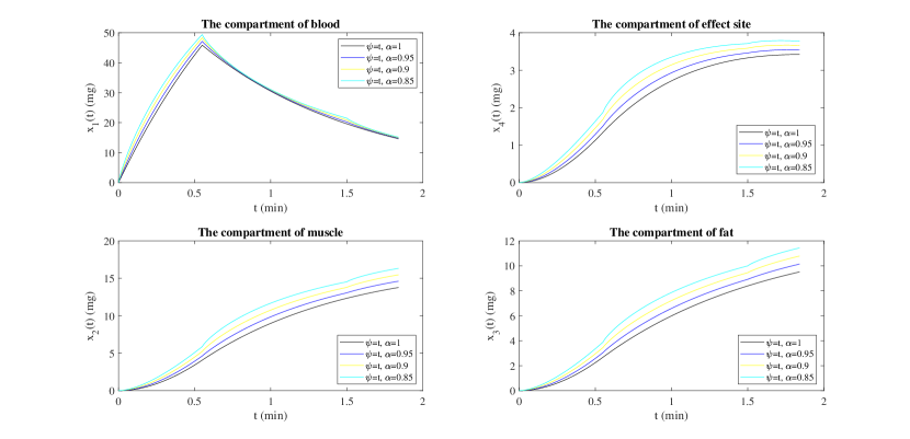
Figure 2: Analysis of the fractional PK/PD model (20) with functions $\psi(t)=t$ for fractional orders $\alpha=1$, $\alpha=0.95$, $\alpha=0.9$ and $\alpha=0.85$.

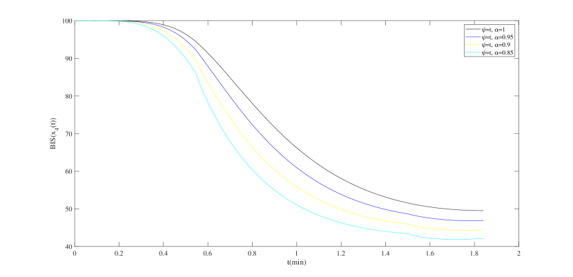
Figure 3: Analysis of controlled BIS with functions $\psi(t)=t$ for fractional orders $\alpha=1$, $\alpha=0.95$, $\alpha=0.9$ and $\alpha=0.85$.

Figure 4 illustrates the solutions of the fractional PK/PD model (20) associated with the functions $\psi(t)=t$, $\psi(t)=\sqrt{t}$, $\psi(t)=t^{2}$, and $\psi(t)=t+0.2$, when considering a fractional order of $\alpha=1$. The graphs shown in Figure 5 depict the controlled BIS corresponding to a specific value of the fractional order $\alpha=1$, under functions $\psi(t)=t$, $\psi(t)=\sqrt{t}$, $\psi(t)=t^{2}$ and $\psi(t)=t+0.2$. It is observed that selecting functions $\psi(t)=\sqrt{t}$ and $\psi(t)=t^{2}$ does not yield satisfactory anesthesia results. On the other hand, employing the functions $\psi(t)=t$ and $\psi(t)=t+0.2$ leads to favorable anesthesia outcomes. In subsequent simulations, we will maintain the functions $\psi(t)=t$ and $\psi(t)=t+0.2$ while altering the fractional orders.

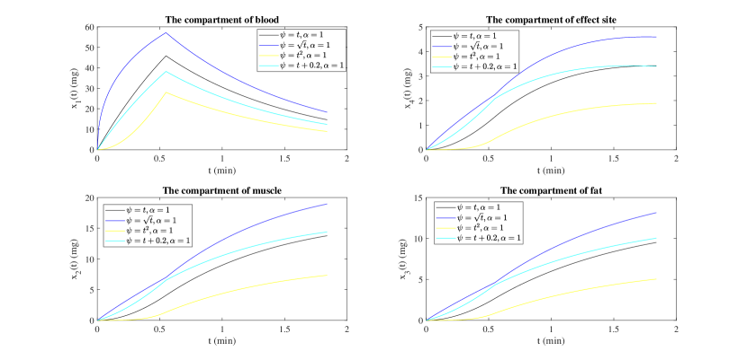
Figure 4: Analysis of the fractional PK/PD model (20) with functions $\psi(t)=t$, $\psi(t)=\sqrt{t}$, $\psi(t)=t^{2}$ and $\psi(t)=t+0.2$ for fractional order $\alpha=1$.

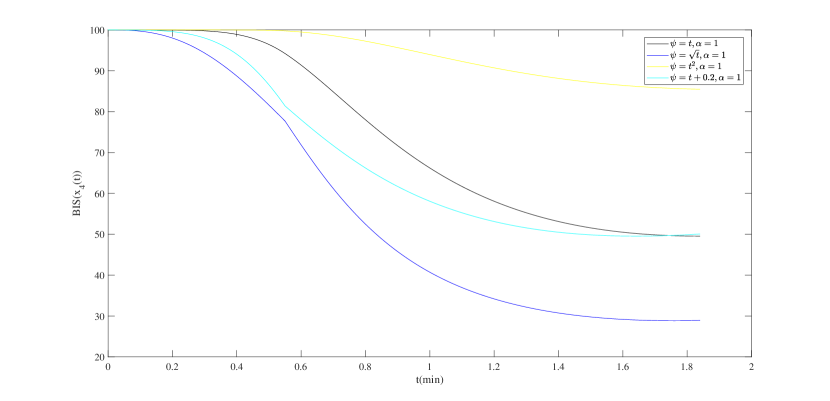
Figure 5: Analysis of controlled BIS with functions $\psi(t)=t$, $\psi(t)=\sqrt{t}$, $\psi(t)=t^{2}$ and $\psi(t)=t+0.2$ for fractional order $\alpha=1$.

In Figure 6, we present the solutions of the fractional PK/PD model (20) corresponding to the functions $\psi(t)=t$ and $\psi(t)=t+0.2$, under the fractional orders $\alpha=1$, $\alpha=0.9$, and $\alpha=0.8$. The curves representing the controlled BIS are displayed in Figure 7. It is worth noting that the recorded BIS values for all fractional orders ranged from 50 (resembling the classical model) to 60, thereby satisfying the condition of anesthesia. However, it is crucial to acknowledge that lower fractional order values, specifically with the function $\psi(t)=t+0.2$, result in a reduced risk of awareness during anesthesia.

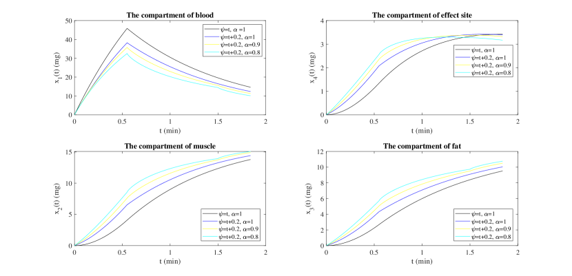
Figure 6: Analysis of the fractional PK/PD model (20) with functions $\psi(t)=t$ and $\psi(t)=t+0.2$ for fractional orders $\alpha=1$, $\alpha=0.9$, and $\alpha=0.8$.

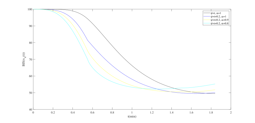
Figure 7: Analysis of controlled BIS with functions $\psi(t)=t$ and $\psi(t)=t+0.2$ for fractional orders $\alpha=1$, $\alpha=0.9$, and $\alpha=0.8$.

4 Discussion

The $\psi$-Caputo fractional PK/PD model represents a notable advancement in modeling due to its ability to capture intricate drug response dynamics, considering the complex relationship between drug concentration and physiological effects. In comparison to conventional modeling approaches, the incorporation of the $\psi$-Caputo fractional derivative and the fractional order $\alpha$ enable a more comprehensive representation of non-local and memory-dependent effects, offering a more nuanced understanding of the induction phase of anesthesia. However, it should be noted that the $\psi$-Caputo fractional PK/PD model is more complex compared to conventional modeling approaches [41, 43] because it relies on fractional calculus and an unknown $\psi$ function, introducing additional parameters, and requires specialized mathematical knowledge. Therefore, its use should be reserved for situations where traditional models are insufficient for capturing the intricacies of the system being modeled with conventional models, based on integer-order calculus, remaining the standard for most PK/PD modeling tasks due to their ease of use and the availability of established methodologies and software [42].

Complex systems often require sophisticated modeling techniques that consider intricate interactions and feedback mechanisms. Additionally, the availability of high-quality data, incorporating a wide range of variables, significantly enhances the reliability of model predictions. Given this, the accuracy and predictability of $\psi$-Caputo fractional PK/PD models are contingent upon the complexity of the research domain and the quality of available data, presenting some limitations: (i) additional parameters; and (ii) data requirements. Indeed, (i) the $\psi$-Caputo model introduces extra parameters associated with the fractional orders, which need to be estimated from data. These additional parameters can make the model more complex and require more data for accurate estimation. (ii) Fractional PK/PD models may require more extensive data to accurately estimate parameters and capture the complexities of the system. Conventional models, in some cases, might work with fewer data points. Moreover, the $\psi$-Caputo fractional PK/PD model inherently carries uncertainties related to the selection of the function $\psi$ and the fractional order $\alpha$, which can impact the model’s reliability in predicting anesthesia dosage. Uncertainties in this model can arise from various sources, e.g. (i) measurement uncertainty (errors in drug concentration measurements can propagate into the model, affecting the accuracy of estimated parameters and predictions), (ii) inter-individual variability (patients can have varying physiological characteristics, which can lead to inter-individual variability in drug response, with the model not capturing all aspects of this variability, potentially resulting in suboptimal dosing for some patients), (iii) intra-individual variability (even within the same individual, the response to anesthesia drugs can vary due to factors like changes in organ function, health status, or concurrent medications, and in that case the $\psi$-Caputo fractional model may not account for all these factors, leading to uncertainty in dosing recommendations for the same patient at different times), (iv) parameter estimation uncertainty (the model relies on various parameters such as clearance, volume of distribution, and rate constants, and estimating these parameters from experimental data can introduce uncertainty), (v) data uncertainty (the quality and quantity of data used to estimate model parameters can vary, and this can lead to uncertainties in the model; sparse or noisy data can result in less reliable model predictions, affecting the accuracy of anesthesia dosage recommendations), (vi) model structure uncertainty (the $\psi$-Caputo fractional PK/PD model itself is a simplification of the complex processes occurring in the body, not fully capturing all relevant mechanisms, leading to uncertainties in predictions). Consequences of these uncertainties in the case of anesthesia (dosage) can be significant: underdosing, if the model underestimates the required dosage, in which case patients may not achieve the desired level of anesthesia, leading to inadequate pain control or awareness during surgery; overdosing, if the model overestimates the required dosage, with patients receiving an excessive anesthesia, leading to complications such as extended recovery times, respiratory depression, or other side effects.

While the $\psi$-Caputo fractional PK/PD model shows advancements in capturing complex drug responses, there might be certain types of drugs or treatments for which this modeling approach may not be as suitable. Some reasons why fractional PK/PD modeling may not be ideal in certain cases include: (i) non-linear pharmacokinetics; (ii) complex drug interactions; (iii) short-acting anesthetics.

Finally, it should be remarked that patient safety must be always of primary importance, especially concerning regulatory aspects like the Bispectral Index (BIS). Any modeling approach should promote patient safety by accurately predicting drug responses and aiding in the development of safer and more effective treatment protocols. Some key aspects on patient safety and the regulation of PKPD models, with a focus on BIS monitoring, are:

• Balancing Technology and Clinical Expertise. While PKPD models and BIS monitoring are valuable tools in anesthesia, they should not replace the judgment and expertise of skilled anesthesiologists. The safe administration of anesthesia requires a combination of technology and clinical acumen.

• Evidence-Based Practice. The development and use of PKPD models and monitoring devices like BIS should be based on rigorous scientific evidence and clinical studies. Regulatory bodies should require strong evidence of safety and efficacy before approving or endorsing these technologies.

• Regulatory Oversight. Regulatory agencies play a crucial role in ensuring that medical devices and models are safe and effective. They should establish and enforce guidelines for the development and use of PKPD models and monitoring devices, including BIS. Regular assessments and updates should be conducted to account for evolving scientific knowledge.

• Continuous Monitoring. Real-time monitoring of patients during surgery is essential for patient safety. Monitoring parameters, including BIS values, should be continuously observed and interpreted by trained personnel to respond promptly to any adverse events or deviations.

• Individualized Care. Each patient is unique, and anesthesia management should be tailored to their specific needs and responses. PKPD models can provide guidance, but individualized care remains central to patient safety.

5 Conclusion

The incorporation of the $\psi$-Caputo fractional derivative in Pharmacokinetics and Pharmacodynamics modeling represents a significant advancement in the field. Indeed, by utilizing fractional-order derivatives, researchers can more accurately capture the complex and non-local behavior observed in drugs within biological systems.

The choice of the function $\psi$ and the fractional order $\alpha$ holds critical importance in modeling the relationship between drug concentrations and pharmacological effects. This approach provides a more realistic representation of drug efficacy and dose-response relationships, allowing for a deeper understanding of the intricate dynamics involved in drug-target interactions.

While our study successfully demonstrates the potential of the $\psi$-Caputo fractional PK/PD model in capturing complex drug responses during the induction phase of anesthesia, it is crucial to acknowledge certain limitations. The current model’s applicability may be constrained by the specific parameters chosen and the simplifications employed to facilitate numerical analysis. Furthermore, the availability of comprehensive clinical data for model validation remains a challenge, which could affect the generalizability of the findings. Future research efforts should focus on addressing these limitations to further enhance the applicability and robustness of the proposed model. Moreover, further research is necessary to explore the impact of the chosen function $\psi$ and the fractional order $\alpha$ on time-delayed responses. This area remains open for investigation, and future studies can delve into understanding how different choices of $\psi$ and $\alpha$ influence the temporal aspects of drug responses.

In summary, the incorporation of $\psi$-Caputo fractional derivatives in Pharmacokinetics and Pharmacodynamics modeling offers valuable insights and advancements. By refining the choice of function $\psi$ and fractional order $\alpha$, researchers can enhance the accuracy and realism of drug modeling, paving the way for a more comprehensive understanding of drug behavior in biological systems.

References

- [1] R. Almeida, A Caputo fractional derivative of a function with respect to another function, Commun Nonlinear Sci Numer Simulat 44 (2017), 460–481.
- [2] M. Arfan et al., On fractional order model of tumor dynamics with drug interventions under nonlocal fractional derivative, Results in Physics 21 (2021), no. 103783, 1–11.
- [3] F. M. Atıcı, M. Atıcı, N. Nguyen, T. Zhoroev and G. Koch, A study on discrete and discrete fractional pharmacokinetics-pharmacodynamics models for tumor growth and anti-cancer effects, Comput. Math. Biophys. 7 (2019), no. 1, 10–24.
- [4] M. S. Avidan et al., Anesthesia awareness and the bispectral index, N Engl J Med. 11 (2008), no. 358, 1097–1108.
- [5] J. M. Bailey and W. M. Haddad, Drug dosing control in clinical pharmacology, IEEE Control Syst. Mag. 25 (2005), no. 2, 35–51.
- [6] D. Baleanu, M. Hasanabadi, A. M. Vaziri and A. Jajarmi, A new intervention strategy for an HIV/AIDS transmission by a general fractional modelling and an optimal control approach, Chaos, Solitons & Fractals 167 (2023), Paper No. 113078, 18 pp.
- [7] C. L. Beck, Modeling and control of Pharmacodynamics, European Journal of Control 24 (2015), 33–49.
- [8] L. L. Brunton, J. S. Lazo and K. L. Parker, The pharmacological basis of therapeutics, 11th ed., McGraw-Hill, New York, 2006.
- [9] D. Copot, R. Magin, R. De Keyser and C. Ionescu, Data-driven modelling of drug tissue trapping using anomalous kinetics, Chaos Solitons Fractals 102 (2017), 441–446.
- [10] E. M. del Amo, P. N. Bishop, P. Godia and L. Aarons, Towards a population pharmacokinetic/pharmacodynamic model of anti-VEGF therapy in patients with age-related macular degeneration, European Journal of Pharmaceutics and Biopharmaceutics, 188 (2023), 78–88.
- [11] A. Dokoumetzidis, A. Iliadis and P. Macheras, Nonlinear Dynamics and Chaos Theory: Concepts and Applications Relevant to Pharmacodynamics, Pharmaceutical Research 18 (2001), 415–426.
- [12] J. Duan and L. Chen, Solution of fractional differential equation systems and computation of matrix Mittag–Leffler functions, Symmetry 10 ( 2018), no. 10, Paper No. 503, 14 pp.
- [13] D. J. Eleveld, P. Colin, A. R. Absalom and M. M. R. F. Struys, Pharmacokinetic-pharmacodynamic model for propofol for broad application in anaesthesia and sedation, British Journal of Anaesthesia 120 (2018), no. 5, 942–959.
- [14] A. S. Evers, M. Maze and E. D. Kharasch, Anesthetic pharmacology: basic principles and clinical practice, 2nd edition, Cambridge University Press, Cambridge, 2011.
- [15] Y. Ferdi et al., Fractional order calculus-based filters for biomedical signal processing, 1st Middle East Conference on Biomedical Engineering, IEEE, 2011.
- [16] J. Gabrielsson and D. Weiner, Pharmacokinetic and Pharmacodynamic Data Analysis: Concepts and Applications, 5th Edition. Stockholm: Swedish Pharmaceutical Press, 2016.
- [17] R. Gorenflo, A. A. Kilbas, F. Mainardi and S. V. Rogosin, Mittag–Leffler Functions, Related Topics and Applications, Springer Monographs in Mathematics, 2014.
- [18] W. M. Haddad, V. Chellaboina and Q. Hui, Nonnegative and compartmental dynamical systems, Princeton Univ. Press, Princeton, NJ, 2010.
- [19] M. Hennion and E. Hanert, How to avoid unbounded drug accumulation with fractional pharmacokinetics, J. Pharmacokin. Pharmacodyn. 40 (2013), no. 6, 691–700.
- [20] C. Ionescu and D. Copot, On the use of fractional order PK-PD models, J. Phys.: Conf. Ser. 783 (2017), Paper No. 012050, 12 pp.
- [21] C. Ionescu, A. Lopes, D. Copot, J. Machado and J. Bates, The role of fractional calculus in modeling biological phenomena: A review, Commun Nonlinear Sci Numer Simul. 51 (2017), 141–159.
- [22] W. P. T. James, Research on obesity: a report of the DHSS/MRC Group, Nutrition Bulletin 4 (1977), no. 3, 187–190.
- [23] F. Jarad and T. Abdeljawad, Generalized fractional derivatives and Laplace transform, Discrete and Continuous Dynamical Systems 13 (2020), no. 3, 709–722.
- [24] S. Joshi, E. Mittal and R. M. Pandey, On Euler type integrals involving extended Mittag-Leffler functions, Bol. Soc. Parana. Mat. 38 (2020), no. 2, 125–134.
- [25] Y. Karaca and D. Baleanu, Algorithmic complexity-based fractional-order derivatives in computational biology, in Advances in mathematical modelling, applied analysis and computation, 55–89, Lect. Notes Netw. Syst., 415, Springer, Singapore, 2023.
- [26] A. A. Kilbas, H. M . Srivastava and J. J. Trujillo, Theory and applications of fractional differential equations, Elsevier Science Limited, 2006.
- [27] F. Li, Incorporating fractional operators into interaction dynamics of a chaotic biological model, Results in Physics 54 (2023), Paper No. 107052, 12 pp.
- [28] R. Magin, Fractional Calculus in Bioengineering (Part 1), Critical Reviews™ in Biomedical Engineering 32 (2004), 1–104.
- [29] B. Meibohm and H. Derendorf, Basic concepts of pharmacokinetic/Pharmacodynamic (PK/PD) modelling, Int. J. Clin. Pharmacol. Ther. 35 (1997), no. 10, 401–413.
- [30] V. F. Morales-Delgado, M.A. Taneco-Hernández, Cruz Vargas-De-León and J.F. Gómez-Aguilar, Exact solutions to fractional pharmacokinetic models using multivariate Mittag-Leffler functions, Chaos, Solitons & Fractals 168 (2023), Paper No. 113164, 15 pp.
- [31] J. D. Morse, L. I. Cortinez and B. J. Anderson, Pharmacokinetic Pharmacodynamic modelling contributions to improve paediatric Anaesthesia practice, J. Clin. Med. 11 (2022), no. 11, Paper No. 3009.
- [32] D. R. Mould and R. N. Upton, Basic Concepts in Population Modeling, Simulation, and Model-Based Drug Development– Part 2: Introduction to Pharmacokinetic Modeling Methods, CPT Pharmacometrics Syst Pharmacol 2 (2013), no. 38.
- [33] E. I. Nielsen and L. E. Friberg, Pharmacokinetic-Pharmacodynamic Modeling of Antibacterial Drugs. Pharmacol Rev. 65 (2013), no. 3, 1053–1090.
- [34] N. Pachauri, J. Yadav, A. Rani and V. Singh, Modified fractional order IMC design based drug scheduling for cancer treatment, Computers in Biology and Medicine 109 (2019), 121–137.
- [35] P. Pandey, J. F. Gómez-Aguilar, M. K. A. Kaabar, Z. Siri and A. A. A. Mousa, Mathematical modeling of COVID-19 pandemic in India using Caputo-Fabrizio fractional derivative, Computers in Biology and Medicine 145 (2022), Paper No. 105518, 8 pp.
- [36] T. W. Schnider, C. F. Minto, P. L. Gambus, C. Andresen, D. B. Goodale, S. L. Shafer and E. J. Youngs, The influence of method of administration and covariates on the pharmacokinetics of propofol in adult volunteers. Anesthesiology 88 (1998), no. 5, 1170–1182.
- [37] S. Singh, D. B. Singh, B. Gautam, A. Singh and N. Yadav, Chapter 19-Pharmacokinetics and pharmacodynamics analysis of drug candidates, Bioinformatics, Academic Press, 305–316, 2022.
- [38] P. Sopasakis, H. Sarimveis, P. Macheras, et al. Fractional calculus in pharmacokinetics, J. Pharmacokinet. Pharmacodyn. 45 (2018), no. 1, 107–125.
- [39] M. Turkyilmazoglu, Hyperthermia therapy of cancerous tumor sitting in breast via analytical fractional model, Computers in Biology and Medicine 164 (2023), Paper No. 107271, 9 pp.
- [40] D. Verotta, Fractional dynamics pharmacokinetics-pharmacodynamic models, J. Pharmacokinet. Pharmacodyn. 37 (2010), no. 3, 257–276.
- [41] S. Zabi, I. Queinnec, G. Garcia and M. Mazerolles, Time-optimal control for the induction phase of anesthesia, IFAC-PapersOnLine 50 (2017), no. 1, 12197–12202.
- [42] S. Zabi, I. Queinnec, S. Tarbouriech, G. Garcia and M. Mazerolles, New approach for the control of anesthesia based on dynamics decoupling, IFAC-PapersOnLine 48 (2015), no. 20, 511–516.
- [43] M. A. Zaitri, C. J. Silva and D. F. M. Torres, An analytic method to determine the optimal time for the induction phase of anesthesia, Axioms 12 (2023), no. 9, Paper No. 867, 15 pp. arXiv:2309.04787