A Deep Learning Method for Simultaneous Denoising and Missing Wedge Reconstruction in Cryogenic Electron Tomography

Abstract

Cryogenic electron tomography (cryo-ET) is a technique for imaging biological samples such as viruses, cells, and proteins in 3D. A microscope collects a series of 2D projections of the sample, and the goal is to reconstruct the 3D density of the sample called the tomogram. This is difficult as the 2D projections have a missing wedge of information and are noisy. Tomograms reconstructed with conventional methods, such as filtered back-projection, suffer from the noise, and from artifacts and anisotropic resolution due to the missing wedge of information. To improve the visual quality and resolution of such tomograms, we propose a deep-learning approach for simultaneous denoising and missing wedge reconstruction called DeepDeWedge. DeepDeWedge is based on fitting a neural network to the 2D projections with a self-supervised loss inspired by noise2noise-like methods. The algorithm requires no training or ground truth data. Experiments on synthetic and real cryo-ET data show that DeepDeWedge achieves competitive performance for deep learning-based denoising and missing wedge reconstruction of cryo-ET tomograms.

1 Introduction

Cryogenic electron tomography (cryo-ET) is a powerful cryo-electron microscopy (cryo-EM) technique for obtaining 3D models of biological samples such as cells and viruses. An important application of cryo-ET is visualizing biological macromolecules like proteins in situ, i.e., in their (close-to) native environment. This preserves biological context, which can greatly improve the understanding of the tasks and workings of the macromolecules [WB16].

In cryo-ET, the sample to be imaged is first prepared on a grid and then frozen. Next, a transmission electron microscope records a tilt series, which is a collection of 2D projections of the sample’s 3D scattering potential or density. Each projection in the tilt series is recorded after tilting the sample for a fixed number of degrees around the microscope’s tilt axis.

From this tilt series, one can estimate a tomogram, i.e., a (discretized) estimate of the sample’s 3D density, using computational techniques. For this inverse problem, numerous approaches have been proposed. The most commonly used tomographic reconstruction technique is filtered back-projection (FBP) [Rad88, WB16, TB20].

Two major obstacles limit the resolution and interpretability of tomograms reconstructed with FBP and similar methods:

1. A missing wedge of information: The range of angles at which useful images can be collected is often limited to, for example, $\pm 60^{\circ}$ rather than the desired full range of $\pm 90^{\circ}$. This is due to the increased thickness of the sample in the direction of the electron beam for tilt angles of large magnitude [Liu+22]. The missing data in the tilt series is wedge-shaped in the Fourier domain.

2. Noisy data: As biological samples studied with cryo-ET are usually sensitive to radiation damage, the total electron dose during tilt series acquisition must be low. Thus, the individual projections of the tilt series have low contrast and a low signal-to-noise ratio (SNR).

In this paper, we propose DeepDeWedge, a deep learning-based imaging approach that simultaneously performs denoising and missing wedge reconstruction. The algorithm takes a single tilt series as input and aims to estimate a noise-free 3D reconstruction of the samples’ density with reconstructed missing wedge. The algorithm can also be applied to a small dataset of tilt-series, typically two to ten, that were collected from samples of the same type, for example, instances of the same cell or solutions containing purified particles, in which case it estimates the noise-free 3D reconstructions, missing-wedge-corrected densities of all the samples.

DeepDeWedge fits a randomly initialized network with a self-supervised loss for simultaneous denoising and missing wedge reconstruction. After fitting, the network is applied to the same data to estimate the tomogram. DeepDeWedge only uses the tilt series of the density we wish to reconstruct and no other training data.

Related methods are effective for denoising and missing wedge reconstruction individually but not simultaneously.

Specifically, IsoNet [Liu+22], a very related deep learning approach for denoising and missing wedge reconstruction, does well at missing wedge reconstruction, but its denoising performance is low compared to state-of-the-art denoising methods [Mal+23]. The current state-of-the-art approaches for denoising in cryo-ET are inspired by noise2noise [Leh+18], a framework for deep-learning-based image denoising. Popular software packages that implement noise2noise-based denoising methods for cryo-ET tomograms are CryoCARE [Buc+19], Topaz [Bep+20] and Warp [TC19]. DeepDeWedge is most related to such noise2noise-based denoising approaches and to IsoNet. We discuss the exact relations in Section 2.1.2 after the description of our algorithm.

DeepDeWedge performs on par with IsoNet on a pure missing wedge reconstruction problem and achieves state-of-the-art denoising performance on a pure denoising problem; on our problem of interest with a missing wedge and a denoising component, it outperforms both IsoNet as well as noise2noise like denoising approaches like CryoCARE.

Our work is also conceptually related to un-trained neural networks, which reconstruct an image or volume based on fitting a neural to data [UVL18, HH18]. Un-trained networks also only rely on fitting a neural network to given measurements. However, they rely on the bias of convolutional neural networks towards natural images [HS20a, HS20], whereas in our setup, we train a network on measurement data to be able to reconstruct from those measurements.

For cryo-EM-related problems other than tomographic reconstruction, deep learning approaches for missing data reconstruction and denoising have also recently been proposed. [Zha+23] proposed a method to restore the state of individual particles inside tomograms, and [LHZ23] proposed a variant of IsoNet to resolve the preferred orientation problem in single-particle cryo-EM [LHZ23].

Another line of works for cryo-ET reconstruction are domain-specific tomographic reconstruction methods that incorporate prior knowledge of biological samples into the reconstruction process to compensate for missing wedge artifacts, for example, ICON [Den+16], and MBIR [Yan+19]. For an overview of such reconstruction methods, we refer readers to the introductory sections of works by [Din+19] and [BBC22]. [Liu+22] compared IsoNet to ICON and MBIR and found that their method outperforms both [Liu+22].

The remainder of this paper is structured as follows: In the remainder of this section, we provide background on cryo-ET. In Section 2.1, we describe the DeepDeWedge algorithm, and Section 2.2 contains experimental results on synthetic and real cryo-ET data.

1.1 Tilt Series Acquisition Model and Problem Statement

A tilt series $\mathbf{t}=\big{(}\mathbf{t}_{-K},\ldots,\mathbf{t}_{K}\big{)}$ is a collection of 2D projections, where each 2D projection $\mathbf{t}_{k}$ is a measurement of an underlying ground truth volume $\mathbf{v}^{*}$ obtained with the electron microscope. The relation of the 2D projections and the ground truth volume is as follows: By the Fourier slice theorem (see e.g. [Mal93]), the 2D Fourier transform $\mathbf{F}\mathbf{t}_{k}$ of each projection image $\mathbf{t}_{k}$ of a tilt series is a noisy observation of a 2D central slice through true volume’s 3D Fourier transform $\mathbf{F}\mathbf{v}^{*}$ multiplied with an additional filter, i.e.,

$$\mathbf{F}\mathbf{t}_{k}=\mathbf{C}_{k}\cdot\mathbf{S}\mathbf{R}_{k}\mathbf{F}\mathbf{v}^{*}+\mathbf{F}\mathbf{\mathbf{n}}_{k}.$$ (1)

In Equation (1), the rotation operator $\mathbf{R}_{k}$ spatially rotates the 3D Fourier transform $\mathbf{F}\mathbf{v}^{*}$ of the volume $\mathbf{v}^{*}$ by the tilt angle $\alpha_{k}$ around the microscope’s tilt axis. Then, the slice-operator $\mathbf{S}$ extracts the central 2D slice of the volume’s Fourier transform that is perpendicular to the microscope’s optical axis. The filter $\mathbf{C}_{k}$ is the contrast transfer function (CTF) of the microscope and models optical aberrations. The term $\mathbf{F}\mathbf{\mathbf{n}}_{k}$ is the Fourier transform of a random 2D image-domain noise term $\mathbf{\mathbf{n}}_{k}$. It is often assumed that the noise $\mathbf{\mathbf{n}}_{k}$ comes from a Poisson distribution (shot noise). Another common assumption is that the Fourier-domain noise $\mathbf{F}\mathbf{\mathbf{n}}_{k}$ is Gaussian, but not necessarily white [BBS20, Fra21]. In this work, we make the weaker assumption that the 2D noise terms $\mathbf{\mathbf{n}}_{k}$ and $\mathbf{\mathbf{n}}_{\ell}$ of any two distinct projections indexed with $k$ and $\ell$ ($k\neq\ell$) have zero means and are independent.

Equation (1) is commonly used as a Fourier-domain model of the image formation process in cryo-EM [Sig16, BBS20]. As the Fourier slice theorem assumes continuous representations of volumes and images, this model is exact only in the continuous case. In this work, we consider discrete representations of volumes and images, as is common in cryo-EM practice. Thus, Equation (1) holds only approximately.

The range of tilt angles $\alpha_{k}$ that yield useful projections $\mathbf{t}_{k}$ is typically limited to, e.g., $\pm 60^{\circ}$ rather than the full range $\pm 90^{\circ}$. Therefore, Equation (1) implies that there is a wedge-shaped region of the sample’s Fourier representation $\mathbf{F}\mathbf{v}^{*}$ which is not covered by any of the Fourier slices $\mathbf{F}\mathbf{t}_{k}$.

We consider the problem of reconstructing a tomogram, i.e., a discretized estimate of a sample’s density from a noisy, incomplete tilt series. This is a difficult inverse problem due to the missing wedge and the high noise level.

2 Results

We now describe our algorithm for estimating missing-wedge corrected, denoised cryo-ET tomograms and evaluate its effectiveness on real and simulated data.

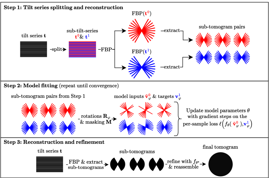
Figure 1: Illustration of DeepDeWedge. To facilitate illustration, we show the 2D tilt series images as 1D Fourier slices and all 3D tomograms as 2D objects in the Fourier domain. Recall that tilt series images, tomograms, and sub-tomograms are objects in the image domain. The figure shows the splitting approach where the tilt series is split into even and odd projections.

2.1 Denoising and missing wedge reconstruction algorithm (DeepDeWedge)

DeepDeWedge takes a single tilt series $\mathbf{t}$ as input and produces a denoised, missing-wedge-filled tomogram. The method can also be applied to a dataset containing multiple (typically up to 10) tilt series from different samples of the same type, for example, a different cell but of the same cell type. DeepDeWedge consists of the following three steps, illustrated in Figure 1:

Step 1: Tilt series splitting and reconstruction. First, split the tilt series $\mathbf{t}$ into two sub-tilt-series ${\color[rgb]{1,0,0}\mathbf{t}^{\text{0}}}$ and ${\color[rgb]{0,0,1}\mathbf{t}^{\text{1}}}$. We propose two approaches to do this: The first is to split the tilt series into even and odd projections based on their order of acquisition. The second splitting approach can be applied if the tilt series is collected using dose fractionation and entails averaging only the even and odd frames recorded at each tilt angle, resulting in two projections per angle.

Next, reconstruct both sub-tilt-series independently with FBP and apply CTF correction. This yields a pair of two coarse reconstructions $\big{(}\text{FBP}({\color[rgb]{1,0,0}\mathbf{t}^{\text{0}}}),\text{FBP}({\color[rgb]{0,0,1}\mathbf{t}^{\text{1}}})\big{)}$ of the sample’s 3D density. Finally, use a 3D-sliding window procedure to extract overlapping cubic sub-tomograms from both FBP reconstructions. The size of these sub-tomogram cubes is a hyper-parameter.

Step 1 produces, say, $N$ paired sub-tomograms extracted from the pair ($\text{FBP}({\color[rgb]{1,0,0}\mathbf{t}^{\text{0}}})$, $\text{FBP}({\color[rgb]{0,0,1}\mathbf{t}^{\text{1}}})$).

Step 2: Model fitting. Fit a randomly initialized network $f_{\text{$\boldsymbol{\theta}$}}$, we use a U-Net [RFB15], with weights $\boldsymbol{\theta}$ by repeating the following steps until convergence:

• Generate model input and target sub-tomograms: For each sub-tomogram pair generated in Step 1, sample a rotation $\mathbf{R}_{\text{$\boldsymbol{\varphi}$}}$ parameterized by the Euler angles $\boldsymbol{\varphi}$ from the uniform distribution on the group of 3D rotations. Construct the model inputs ${\color[rgb]{1,0,0}\tilde{\mathbf{v}}_{{\color[rgb]{0,0,0}\text{$\boldsymbol{\varphi}$}}}^{\text{0}}}$ and targets ${\color[rgb]{0,0,1}\mathbf{v}_{{\color[rgb]{0,0,0}\text{$\boldsymbol{\varphi}$}}}^{\text{1}}}$ by applying the rotation $\mathbf{R}_{\text{$\boldsymbol{\varphi}$}}$ to both sub-tomograms and adding an artificial missing wedge to the rotated sub-tomogram from the FBP reconstruction of the even tilt series. The missing wedge is added by taking the Fourier transform of the rotated sub-tomograms and multiplying them with a binary 3D mask $\mathbf{M}$ that zeros out all Fourier components that lie inside the missing wedge. We generate one input-target pair with Euler angles $\boldsymbol{\varphi}$ for each of the $N$ sub-tomogram pairs from Step 1. This yields a set of $N$ triplets consisting of model input, target sub-tomogram, and angle $\big{\{}\big{(}{\color[rgb]{1,0,0}\tilde{\mathbf{v}}_{{\color[rgb]{0,0,0}\text{$\boldsymbol{\varphi}$}}}^{\text{0}}},{\color[rgb]{0,0,1}\mathbf{v}_{{\color[rgb]{0,0,0}\text{$\boldsymbol{\varphi}$}}}^{\text{1}}},\text{$\boldsymbol{\varphi}$}\big{)}_{0},\ldots,\big{(}{\color[rgb]{1,0,0}\tilde{\mathbf{v}}_{{\color[rgb]{0,0,0}\text{$\boldsymbol{\varphi}$}}}^{\text{0}}},{\color[rgb]{0,0,1}\mathbf{v}_{{\color[rgb]{0,0,0}\text{$\boldsymbol{\varphi}$}}}^{\text{1}}},\text{$\boldsymbol{\varphi}$}\big{)}_{N}\big{\}}$.

• Update the model: Update the model weights $\boldsymbol{\theta}$ by performing gradient steps with the per-sample loss

  $$\ell\left(f_{\text{$\boldsymbol{\theta}$}}\left({\color[rgb]{1,0,0}\tilde{\mathbf{v}}_{{\color[rgb]{0,0,0}\text{$\boldsymbol{\varphi}$}}}^{\text{0}}}\right),{\color[rgb]{0,0,1}\mathbf{v}_{{\color[rgb]{0,0,0}\text{$\boldsymbol{\varphi}$}}}^{\text{1}}},\text{$\boldsymbol{\varphi}$}\right)=\left|\left|\left(\mathbf{M}\mathbf{M}_{\text{$\boldsymbol{\varphi}$}}+2\mathbf{M}^{C}\mathbf{M}_{\text{$\boldsymbol{\varphi}$}}\right)\mathbf{F}\left(f_{\text{$\boldsymbol{\theta}$}}\big{(}{\color[rgb]{1,0,0}\tilde{\mathbf{v}}_{{\color[rgb]{0,0,0}\text{$\boldsymbol{\varphi}$}}}^{\text{0}}}\big{)}-{\color[rgb]{0,0,1}\mathbf{v}_{{\color[rgb]{0,0,0}\text{$\boldsymbol{\varphi}$}}}^{\text{1}}}\right)\right|\right|_{2}^{2}.$$ (2)

  Here, $\mathbf{M}_{\text{$\boldsymbol{\varphi}$}}$ is the rotated version of the wedge mask $\mathbf{M}$ and $\mathbf{M}^{C}:=\mathbf{I}-\mathbf{M}$ is the complement of the mask. For the gradient updates, we use the Adam [KB15] optimizer and perform a single pass through the $N$ model input and target sub-tomograms generated before.

Step 3: Reconstruction and refinement. Reconstruct the full, non-splitted tilt series $\mathbf{t}$ using FBP. Then, like in Step 1, split it into sub-tomograms and refine the sub-tomograms by passing them through the fitted network $f_{\text{$\boldsymbol{\theta}$}^{*}}$ from Step 2. Finally, reassemble the refined sub-tomograms to obtain the final denoised and missing-wedge-corrected tomogram.

2.1.1 Motivation for the three steps of the algorithm

Motivation for Step 1: We split the tilt series into two disjoint parts to obtain measurements with independent noise. As the noise on the individual projections or frames is assumed to be independent, the reconstructions $\text{FBP}({\color[rgb]{1,0,0}\mathbf{t}^{\text{0}}})$ and $\text{FBP}({\color[rgb]{0,0,1}\mathbf{t}^{\text{1}}})$ are noisy observations of the same underlying sample with independent noise terms. Those are used in Step 2 for the self-supervised noise2noise-inspired loss.

Tilt series splitting is also used in popular implementations of noise2noise-like denoising methods for cryo-ET [Buc+19, Bep+20, TC19]. The frame-based splitting procedure was proposed by [Buc+19], who found that it can improve the performance of noise2noise-like denoising over the even/odd split.

Splitting the FBP reconstruction into smaller sub-tomograms is necessary since full tomograms are typically too large to be used for the model fitting in Step 2. The size of these sub-tomograms is a hyperparameter. Experiments on synthetic data suggest that larger sub-tomograms tend to yield better results (see Appendix D.1).

Motivation for Step 2: A brief justification for the loss function is as follows; a detailed motivation is in Section 2.1.3.

As the masks $\mathbf{M}\mathbf{M}_{\text{$\boldsymbol{\varphi}$}}$, and $\mathbf{M}^{C}\mathbf{M}_{\text{$\boldsymbol{\varphi}$}}$ are orthogonal, the per-sample loss $\ell$ in Equation (2) can be expressed as the sum of two the two terms $\left|\left|\mathbf{M}\mathbf{M}_{\text{$\boldsymbol{\varphi}$}}\mathbf{F}\left(f_{\text{$\boldsymbol{\theta}$}}\left({\color[rgb]{1,0,0}\tilde{\mathbf{v}}_{{\color[rgb]{0,0,0}\text{$\boldsymbol{\varphi}$}}}^{\text{0}}}\right)-{\color[rgb]{0,0,1}\mathbf{v}_{{\color[rgb]{0,0,0}\text{$\boldsymbol{\varphi}$}}}^{\text{1}}}\right)\right|\right|_{2}^{2}$, and $\left|\left|2\mathbf{M}^{C}\mathbf{M}_{\text{$\boldsymbol{\varphi}$}}\mathbf{F}\left(f_{\text{$\boldsymbol{\theta}$}}\left({\color[rgb]{1,0,0}\tilde{\mathbf{v}}_{{\color[rgb]{0,0,0}\text{$\boldsymbol{\varphi}$}}}^{\text{0}}}\right)-{\color[rgb]{0,0,1}\mathbf{v}_{{\color[rgb]{0,0,0}\text{$\boldsymbol{\varphi}$}}}^{\text{1}}}\right)\right|\right|_{2}^{2}$. The first summand, i.e., $\left|\left|\mathbf{M}\mathbf{M}_{\text{$\boldsymbol{\varphi}$}}\mathbf{F}\left(f_{\text{$\boldsymbol{\theta}$}}\left({\color[rgb]{1,0,0}\tilde{\mathbf{v}}_{{\color[rgb]{0,0,0}\text{$\boldsymbol{\varphi}$}}}^{\text{0}}}\right)-{\color[rgb]{0,0,1}\mathbf{v}_{{\color[rgb]{0,0,0}\text{$\boldsymbol{\varphi}$}}}^{\text{1}}}\right)\right|\right|_{2}^{2}$, is the squared L2 distance between the network output and the target sub-tomogram ${\color[rgb]{0,0,1}\mathbf{v}_{{\color[rgb]{0,0,0}\text{$\boldsymbol{\varphi}$}}}^{\text{1}}}$ on all Fourier components that were not masked out by the two missing wedge masks $\mathbf{M}$ and $\mathbf{M}_{\text{$\boldsymbol{\varphi}$}}$. As we assume the noise in the target to be independent of the noise in the input ${\color[rgb]{1,0,0}\tilde{\mathbf{v}}_{{\color[rgb]{0,0,0}\text{$\boldsymbol{\varphi}$}}}^{\text{0}}}$, minimizing this part incentivizes the network to learn to denoise these Fourier components. This is inspired by the noise2noise principle.

The second summand, i.e., $\left|\left|2\mathbf{M}^{C}\mathbf{M}_{\text{$\boldsymbol{\varphi}$}}\mathbf{F}\left(f_{\text{$\boldsymbol{\theta}$}}\left({\color[rgb]{1,0,0}\tilde{\mathbf{v}}_{{\color[rgb]{0,0,0}\text{$\boldsymbol{\varphi}$}}}^{\text{0}}}\right)-{\color[rgb]{0,0,1}\mathbf{v}_{{\color[rgb]{0,0,0}\text{$\boldsymbol{\varphi}$}}}^{\text{1}}}\right)\right|\right|_{2}^{2}$, can be interpreted as a noisier2noise-like loss (see Section A.2 for background), and it incentivizes the network $f_{\text{$\boldsymbol{\theta}$}}$ to restore the data that we artificially removed with the mask $\mathbf{M}$. For this part, it is important that we rotate both volumes, which move their original missing wedges to a new, random location.

Motivation for Step 3: The model inputs during fitting, i.e., sub-tomograms of FBP reconstructions of the sub-tilt-series ${\color[rgb]{1,0,0}\mathbf{t}^{\text{0}}}$ have an additional missing wedge introduced by the mask $\mathbf{M}$. Thus, the model is fitted to reconstruct more data than what is masked out by the original missing wedge. In Step 3, we nevertheless apply the model to the data with only the original missing wedge missing. We found empirically that applying the model to sub-tomograms of the full, non-corrupted FBP reconstruction yields very similar performance compared to applying it to multiple inputs used for model fitting and averaging them. Applying the model to the full FBP reconstruction is computationally much cheaper and, moreover, deterministic since it requires no random sampling and averaging.

2.1.2 Related methods

As mentioned before, DeepDeWedge is closely related to Noise2Noise-based denoising methods and the denoising and missing wedge-filling method IsoNet [Liu+22].

Relation to Noise2Noise-Like Denoising in Cryo-ET.

Noise2noise-like methods for cryo-ET as implemented in CryoCARE [Buc+19] or Warp [TC19] take one or more tilt series as input and return denoised tomograms. A randomly initialized network $f_{\text{$\boldsymbol{\theta}$}}$ is fitted for denoising on sub-tomograms of FBP reconstructions $\text{FBP}({\color[rgb]{1,0,0}\mathbf{t}^{\text{0}}})$ and $\text{FBP}({\color[rgb]{0,0,1}\mathbf{t}^{\text{1}}})$ of sub-tilt-series ${\color[rgb]{1,0,0}\mathbf{t}^{\text{0}}}$ and ${\color[rgb]{0,0,1}\mathbf{t}^{\text{1}}}$ obtained from a full tilt series $\mathbf{t}$. The model is fitted by minimizing a loss function (typically the mean-squared error), between the output of the model $f_{\text{$\boldsymbol{\theta}$}}$ applied to one noisy sub-tomogram and the corresponding other noisy sub-tomogram. The fitted model is then used to denoise the two reconstructions $\text{FBP}({\color[rgb]{1,0,0}\mathbf{t}^{\text{0}}})$ and $\text{FBP}({\color[rgb]{0,0,1}\mathbf{t}^{\text{1}}})$, which are then averaged to obtain the final denoised tomogram.

Contrary to the denoising methods above, DeepDeWedge fits a network that is incentivized to not only denoise but also to fill the missing wedge.

Relation to IsoNet.

IsoNet takes a small set of, say, one to ten tomograms, and produces denoised, missing-wedge corrected versions of those tomograms. Similar as for our approach, a randomly initialized network is fitted for denoising and missing wedge reconstruction on sub-tomograms of these tomograms, however the fitting process is quite different. Inspired by noisier2noise, the model is fitted on the task of mapping sub-tomograms that are further corrupted with an additional missing wedge and additional noise onto their non-corrupted versions. After each iteration, the intermediate model is used to predict the content of the original missing wedges of all sub-tomograms. The predicted missing wedge content is inserted into all sub-tomograms, which serve as input to the next iteration of the algorithm.

Contrary, our denoising approach is noise2noise-like, as in CryoCARE. This leads to better performance, as we will see later, as well as requiring fewer assumptions and no hyperparameter tuning. Specifically, noisier2noise-like denoising requires knowledge of the noise model and strength (see Appendix A.2). As this knowledge is typically unavailable, [Liu+22] propose approximate noise models from which the user has to choose. After model fitting, the user must manually decide which iteration and noise level gave the best reconstruction. Thus, IsoNet’s noisier2noise-inspired denoising approach requires several hyperparameters for which good values exist but are unknown. Therefore, IsoNet requires tuning to achieve good results. Our denoising approach introduces no additional hyperparameters and does not require knowledge of the noise model and strength.

The commonality between our approach and IsoNet is the noisier2noise-like mechanism for missing wedge reconstruction, which consists of artificially removing another wedge from the sub-tomograms and fitting the model to reconstruct the wedge.

2.1.3 Theoretical Motivation

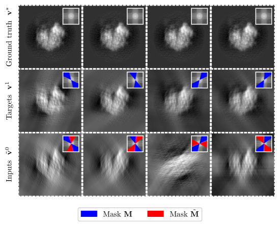
Figure 2: Illustration of a ground-truth structure $\mathbf{v}^{*}$, and corresponding model targets ${\color[rgb]{0,0,1}\mathbf{v}_{{\color[rgb]{0,0,0}}}^{\text{1}}}$ and inputs ${\color[rgb]{1,0,0}\mathbf{v}_{{\color[rgb]{0,0,0}}}^{\text{0}}}$ for the setup of our theoretical motivation. We visualize a 2D structure with no additive noise and random in-plane rotations for simplicity. The small inset boxes in each patch show the absolute values of the Fourier transforms of the images and regions that are zeroed out by the missing wedge masks.

Here, we present a theoretical result that motivates the choice of our per-sample loss $\ell$ defined in Equation (2). We consider an idealized setup that deviates from practice to motivate our loss.

We assume access to data that consists of many noisy, missing-wedge-affected 3D observations of a fixed ground truth 3D structure $\mathbf{v}^{*}\in\mathbb{R}^{N\times N\times N}$. Specifically, data is generated as two measurements (in the form of volumes) of the unknown ground-truth volume of interest, $\mathbf{v}^{*}$, as

$${\color[rgb]{1,0,0}\mathbf{v}_{{\color[rgb]{0,0,0}}}^{\text{0}}}=\mathbf{F}^{-1}\mathbf{M}\mathbf{F}\big{(}\mathbf{v}^{*}+\mathbf{{\color[rgb]{1,0,0}\mathbf{n}^{\text{0}}}}\big{)},\qquad{\color[rgb]{0,0,1}\mathbf{v}_{{\color[rgb]{0,0,0}}}^{\text{1}}}=\mathbf{F}^{-1}\mathbf{M}\mathbf{F}\big{(}\mathbf{v}^{*}+\mathbf{{\color[rgb]{0,0,1}\mathbf{n}^{\text{1}}}}\big{)},$$ (3)

where $\mathbf{{\color[rgb]{1,0,0}\mathbf{n}^{\text{0}}}},\mathbf{{\color[rgb]{0,0,1}\mathbf{n}^{\text{1}}}}\in\mathbb{R}^{N\times N\times N}$ are random noise terms and $\mathbf{M}\in\{0,1\}^{N\times N\times N}$ is the missing wedge mask. From the first measurement, we generate a noisier observation ${\color[rgb]{1,0,0}\tilde{\mathbf{v}}_{{\color[rgb]{0,0,0}}}^{\text{0}}}=\mathbf{F}^{-1}\mathbf{{\color[rgb]{0,0,0}\tilde{M}}}\mathbf{F}{\color[rgb]{1,0,0}\mathbf{v}_{{\color[rgb]{0,0,0}}}^{\text{0}}}$ by applying a second missing wedge mask $\mathbf{{\color[rgb]{0,0,0}\tilde{M}}}$. The noisier observation has two missing wedges: the wedge introduced by the first and the wedge introduced by the second mask. We assume that the two masks follow a joint and symmetric distribution. An example of a choice of such distributions is that for each mask, a random wedge is chosen uniformly at random.

Figure 2 illustrates a few datapoints in 2D. The top row shows four identical copies of a ground truth structure $\mathbf{v}^{*}$. The second row shows missing wedge-corrupted versions of the ground truth. For clarity, we set the additive noise terms $\mathbf{{\color[rgb]{1,0,0}\mathbf{n}^{\text{0}}}}$ and $\mathbf{{\color[rgb]{0,0,1}\mathbf{n}^{\text{1}}}}$ to zero, which implies ${\color[rgb]{1,0,0}\mathbf{v}_{{\color[rgb]{0,0,0}}}^{\text{0}}}={\color[rgb]{0,0,1}\mathbf{v}_{{\color[rgb]{0,0,0}}}^{\text{1}}}$. The last row shows noisier observations ${\color[rgb]{1,0,0}\tilde{\mathbf{v}}_{{\color[rgb]{0,0,0}}}^{\text{0}}}$ of the samples in the second row, which are corrupted by two missing wedges.

We then train a neural network $f_{\text{$\boldsymbol{\theta}$}}$ to minimize the loss

$$\mathcal{L}(\text{$\boldsymbol{\theta}$})=\mathop{\mathbb{E}}_{\mathbf{M},\mathbf{{\color[rgb]{0,0,0}\tilde{M}}},{\color[rgb]{1,0,0}\mathbf{n}^{\text{0}}},{\color[rgb]{0,0,1}\mathbf{n}^{\text{1}}}}\left[\left|\left|\big{(}\mathbf{{\color[rgb]{0,0,0}\tilde{M}}}\mathbf{M}+2\mathbf{{\color[rgb]{0,0,0}\tilde{M}}}^{C}\mathbf{M}\big{)}\mathbf{F}\Big{(}f_{\text{$\boldsymbol{\theta}$}}\big{(}{\color[rgb]{1,0,0}\tilde{\mathbf{v}}_{{\color[rgb]{0,0,0}}}^{\text{0}}}\big{)}-{\color[rgb]{0,0,1}\mathbf{v}_{{\color[rgb]{0,0,0}}}^{\text{1}}}\Big{)}\right|\right|_{2}^{2}\right],$$ (4)

where the expectation is over the random masks and the noise term. Note that this resembles training on infinitely many data points, with a very similar loss than the original loss (2); the main difference is that in the original loss, the volume is rotated randomly but the mask $\mathbf{M}$ is fixed, while in the setup considered in this section, the volume is fixed but the masks $\mathbf{M}$ and $\mathbf{{\color[rgb]{0,0,0}\tilde{M}}}$ are random.

After training, we can use the network to estimate the ground-truth volume by applying the network to another noisy observation ${\color[rgb]{1,0,0}\tilde{\mathbf{v}}_{{\color[rgb]{0,0,0}}}^{\text{0}}}$. The following proposition establishes that this is equivalent to training the network on a supervised loss to reconstruct the loss ${\color[rgb]{1,0,0}\tilde{\mathbf{v}}_{{\color[rgb]{0,0,0}}}^{\text{0}}}$, provided the two masks are non-overlapping.

Proposition 1.

Assume that the noise $\mathbf{{\color[rgb]{0,0,1}\mathbf{n}^{\text{1}}}}$ is zero-mean and independent of the noise $\mathbf{{\color[rgb]{1,0,0}\mathbf{n}^{\text{0}}}}$, and of the masks $(\mathbf{M},\mathbf{{\color[rgb]{0,0,0}\tilde{M}}})$, and assume that the noise $\mathbf{{\color[rgb]{1,0,0}\mathbf{n}^{\text{0}}}}$ is also independent of the masks. Moreover, assume that the joint probability distribution $P$ of the missing wedge masks $\mathbf{M}$ and $\mathbf{{\color[rgb]{0,0,0}\tilde{M}}}$ is symmetric, i.e., $P(\mathbf{M},\mathbf{{\color[rgb]{0,0,0}\tilde{M}}})=P(\mathbf{{\color[rgb]{0,0,0}\tilde{M}}},\mathbf{M})$, and that the missing wedges do not overlap. Then the loss $\mathcal{L}$ is proportional to the supervised loss

$$\mathcal{R}(\text{$\boldsymbol{\theta}$})=\mathop{\mathbb{E}}_{\mathbf{M},\mathbf{{\color[rgb]{0,0,0}\tilde{M}}},{\color[rgb]{1,0,0}\mathbf{n}^{\text{0}}}}\left[\left|\left|f_{\text{$\boldsymbol{\theta}$}}\big{(}\mathbf{{\color[rgb]{1,0,0}\tilde{\mathbf{v}}_{{\color[rgb]{0,0,0}}}^{\text{0}}}}\big{)}-\mathbf{\mathbf{v}_{missing}^{*}}\right|\right|_{2}^{2}\right],$$ (5)

i.e., $\mathcal{L}(\text{$\boldsymbol{\theta}$})=\mathcal{R}(\text{$\boldsymbol{\theta}$})+c,$ where $c$ is a numerical constant independent of the network parameters $\boldsymbol{\theta}$.

The proof of Proposition 1 is in Appendix B, where we consider the more general case where the masks $\mathbf{M}$ and $\mathbf{{\color[rgb]{0,0,0}\tilde{M}}}$ may overlap, resulting in a slightly different supervised loss $\mathcal{R}$.

In practice, we do not apply our approach to the problem of reconstructing a single fixed structure $\mathbf{v}^{*}$ from multiple pairs of noisy observations with random missing wedges. Instead, we consider the problem of reconstructing several unique biological samples using a small dataset of tilt series. To this end, we fit a model with an empirical estimate of a risk similar to the one considered in Proposition 1. We fit the model on sub-tomogram pairs extracted from the FBP reconstructions of the even and odd sub-tilt-series, which exhibit independent noise. Moreover, as already mentioned above, in the setup of our algorithm, the two missing wedge masks $\mathbf{M}$ and $\mathbf{{\color[rgb]{0,0,0}\tilde{M}}}$ themselves are not random. However, as we randomly rotate the model input sub-tomograms during model fitting, the missing wedges appear at a random location with respect to an arbitrary fixed orientation of the sub-tomogram.

2.2 Experiments

We now demonstrate the performance of DeepDeWedge on real and synthetic data. We begin with experiments on two real-world datasets and then perform experiments on synthetic data in order to quantify performance differences between our method, IsoNet, and CryoCARE.

2.2.1 Experiments on Purified S. Cerevisiae 80S Ribosomes (EMPIAR-10045)

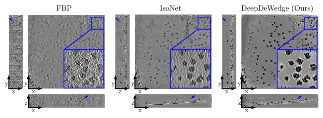
Figure 3: Slices through 3D reconstructions of a tomogram containing purified S. cerevisiae 80S ribosomoes (EMPIAR-10045, Tomogram 5). To improve contrast, we normalized all tomograms and clamped their maximum and minimum voxel values to +/- three times the standard deviation.

The first dataset we consider is EMPIAR-10045, the tutorial dataset for sub-tomogram averaging in Relion [BS16]. We chose this dataset because it is commonly used to test new algorithms, for example, to evaluate IsoNet [Liu+22].

Dataset: EMPIAR-10045 is publicly available through the Electron Microscopy Public Image Archive (EMPIAR). It contains 7 tilt series collected from samples of purified S. Cerevisiae 80S Ribosomes. All tilt series are aligned and consist of 41 projections collected at tilt angles from $-60^{\circ}$ to $+60^{\circ}$ with $3^{\circ}$ increment. The original pixel size of the projections is 2.17 Å. After FBP reconstruction, we binned all tomograms 6 times, resulting in a cubic voxel size of $13.02$ Å. We applied IsoNet’s Wiener-filter-based CTF correction to all tomograms and finally extracted around 420 sub-tomograms extracted with shape $80\times 80\times 80$ for model fitting.

Network Architecture: We compare to IsoNet and FBP. For both IsoNet and our method, we used a U-Net [RFB15] with 64 channels and 3 downsampling layers. The network has $27.3$ million trainable parameters and is also the default model architecture of IsoNet. For IsoNet, we used the original IsoNet implementation (https://github.com/IsoNet-cryoET/IsoNet). By default, IsoNet uses regularization with dropout with probability $0.3$. For our method, dropout is not necessary and increases the fitting time, so we do not use dropout for our method.

Results: Figure 3 shows tomograms refined with IsoNet and DeepDeWedge using the even/odd tilt series splitting approach. Both IsoNet and our method drastically reduce the missing wedge effects and eliminate the artificial elongations of the ribosomes in the z-direction, as can be seen from the slices through the tomogram parallel to the x-z-plane (bottom panels). In this plane, the performance between IsoNet and our method is quite similar. We find that our method yields a much less noisy reconstruction compared to compared to IsoNet. Our reconstruction shows some details that are barely visible in the IsoNet reconstruction (blue pointers) and achieves higher contrast.

2.2.2 Experiments on Flagella of Chlamydomonas Reinhardtii

We now evaluate our algorithm on a second real-world dataset, the tutorial dataset for CryoCARE that is available online (see https://github.com/juglab/cryoCARE_T2T). Besides comparing our method to IsoNet, we also investigate the impact of the choice of the CTF correction method on the quality of the reconstructions.

[Mal+23] observed that the Wiener-filter-based CTF correction proposed by [Liu+22] for use with IsoNet yields slightly blurry reconstructions in which some details are washed out. Therefore, we compare the performance of IsoNet and our method when applied to data treated with either Wiener-filter-based CTF correction or the commonly used phase flipping method [Zan+09].

Dataset: The dataset consists of a single tilt series collected from the flagella of Chlamydomonas reinhardtii. The projections were collected at angles from $-65^{\circ}$ to $+65^{\circ}$ with $2^{\circ}$ increment. Each projection was acquired using dose fractionation with $10$ frames per tilt angle. Each frame has a pixel size of $2.36$ Å. Again, a binning factor of 6 was used for reconstruction, resulting in a voxel size of $14.16$ Å.

As IsoNet is optimized for a missing wedge of $60^{\circ}$, we artificially widened the missing wedge from the original $50^{\circ}$ to $60^{\circ}$ by multiplying the reconstruction with a missing wedge filter in the Fourier domain for a fair comparison. Finally, we extracted around 150 sub-tomograms with shape $96\times 96\times 96$ for model fitting.

Results: The reconstructions obtained with IsoNet and our method, again using the even/odd tilt series split, are shown in Figure 4. When CTF correction is done with the Wiener filter (top row), our method yields better denoising performance than IsoNet while performing similarly for missing wedge reconstruction. The second row shows the final volumes when CTF correction is done via phase flipping with IMOD. Note that the Wiener filter results in a less noisy FBP reconstruction with higher contrast. [Liu+22] already noted that IsoNet performs better when applied to higher contrast volumes, which we find confirmed. For all methods, the Wiener-filter-based CTF-correction results in smoother and blurrier reconstructions in which some high-frequency details are washed out (see zoomed-in region), which agrees with the observations of [Mal+23].

As the tilt series was collected using dose fractionation, we also applied DeepDeWedge with the frame-based splitting approach, which yielded a reconstruction with more high-frequency details but slightly less contrast compared to the even/odd split. See Appendix D.4 for more details.

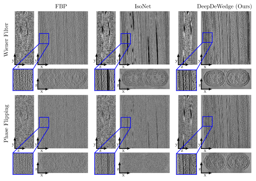
Figure 4: Slices through 3D reconstructions of the flagella of Chlamydomonas reinhardtii obtained with different methods and with different CTF correction.

2.2.3 Experiments on Synthetic Data

On the real-world data, we observed that DeepDeWedge performs similar to IsoNet for missing wedge reconstruction but has improved denoising performance, which yields overall better image quality. To quantify this, we compare our method to IsoNet and CryoCARE on synthetic data and find that our method outperforms both; specifically, the missing wedge reconstruction performance is on par with IsoNet, and the denoising performance is on par with CryoCARE, and the overall reconstruction quality is superior to both.

Dataset: We used a dataset by [Gub+20] containing 10 noiseless synthetic ground truth volumes with a spatial resolution of 10 ų/voxel and a size of $179\times 512\times 512$ voxels. All volumes contain typical objects found in cryo-ET samples, such as proteins (up to 1,500 uniformly rotated samples from a set of 13 structures), membranes, and gold fiducial markers. We selected the first three tomograms and used the Python library tomosipo [Hen+21] to compute clean projections of size $512\times 512$ in the angular range $\pm 60^{\circ}$ with $2^{\circ}$ increment, which results in a missing wedge of $60^{\circ}$. From these clean tilt series, we generated datasets with different noise levels by adding pixel-wise independent Gaussian noise to the projections. We simulated three datasets with tilt-series SNR $1/2$, $1/4$, and $1/6$, respectively. We used 150 sub-tomograms of size $96\times 96\times 96$ to fit all models.

Network Architecture and Optimizer: For all three methods (CryoCARE, IsoNet, and DeepDeWedge), we used the same U-Net described above. For CryoCARE, we used our own implementation since CryoCARE can be obtained from our algorithm by omitting the masking and rotation steps. We found that dropout and early stopping is necessary for cryoCARE to prevent overfitting. Again, for our DeepDeWedge, dropout is not necessary and slightly decreases performance, but we still used it for the sake of comparability

Evaluation Metrics: To measure the overall quality of a tomogram $\hat{\mathbf{v}}$ obtained with any of the three methods, we calculated the normalized correlation coefficient $\text{CC}(\hat{\mathbf{v}},\mathbf{v}^{*})$ between the reconstruction $\hat{\mathbf{v}}$ and the corresponding ground-truth $\mathbf{v}^{*}$, which is defined as

$$\text{CC}(\hat{\mathbf{v}},\mathbf{v}^{*})=\frac{\big{\langle}\hat{\mathbf{v}}-\text{mean}(\hat{\mathbf{v}}),\mathbf{v}^{*}-\text{mean}(\mathbf{v}^{*})\big{\rangle}}{\left|\left|\hat{\mathbf{v}}-\text{mean}(\hat{\mathbf{v}})\right|\right|_{2}\left|\left|\hat{\mathbf{v}}-\text{mean}(\hat{\mathbf{v}})\right|\right|_{2}}.$$ (6)

By definition, it holds that $0\leq\text{CC}(\hat{\mathbf{v}},\mathbf{v}^{*})\leq 1$, and the higher the correlation between reconstruction and ground truth, the better. The correlation coefficient measures the reconstruction quality (both the denoising and the missing wedge reconstruction capabilities) of the methods. To isolate the denoising performance of a method from its ability to reconstruct the missing wedge, we also report the correlation coefficient between the refined reconstructions and the ground truth after applying a $60^{\circ}$ missing wedge filter to both of them. We refer to this metric as CC outside the missing wedge and it is used to compare to the denoising performance of CryoCARE, which does not perform missing wedge reconstruction.

As a central application of cryo-ET is the analysis of biomolecules, we also report the resolution of all proteins in the refined tomograms. For this, we extracted all proteins from the ground truth and refined tomograms and calculated the average 0.143 Fourier shell correlation cutoff (0.143-FSC) between the refined proteins and the ground truth ones. The 0.143-FSC is commonly used in cryo-EM applications. Its unit is Angstroms, and it seeks to express up to which spatial frequency the information in the reconstruction is reliable. In contrast to the correlation coefficient, a lower 0.143-FSC value is better. To measure how well each method filled in the missing wedges of the structures, we also report the average 0.143-FSC calculated only on the true and predicted missing wedge data. We refer to this value as (average) 0.143-FSC inside the missing wedge.

Results: Figure 5 shows the metrics for decreasing SNR of the tilt series. The correlation coefficients suggest that DeepDeWedge yields higher-quality reconstructions than IsoNet and CryoCARE.

CryoCARE achieves a lower correlation coefficient than IsoNet in the high-SNR regime, while the order is reversed for low SNR. A likely explanation is that for lower noise levels, the correlation coefficient is more sensitive to the missing wedge artifacts in the reconstructions. CryoCARE does not perform missing wedge reconstruction, so it has a lower correlation coefficient than IsoNet for higher SNR. For lower SNR, the correlation coefficient is dominated by the noise. Regarding denoising, it has been observed that CryoCARE has better performance than IsoNet [Mal+23], which is confirmed here by looking at the correlation coefficient outside the missing wedge. DeepDeWedge performs denoising and missing-wedge filling and thus outperforms both methods. The perceived quality of the reconstructions shown in Figure 6 agrees with the metric-based comparison.

The FSC metrics in the second row of Figure 5 indicate that the average resolution of the proteins in the refined tomograms is approximately the same for IsoNet and DeepDeWedge and that they perform similarly for missing wedge reconstruction.

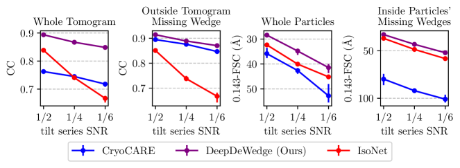
Figure 5: Comparison of our method (with even/odd split) to IsoNet and CryoCARE for increasing noise levels on the tilt series images. The circular markers are the mean values of three runs with different randomness, while the bars indicate the best and worst runs.

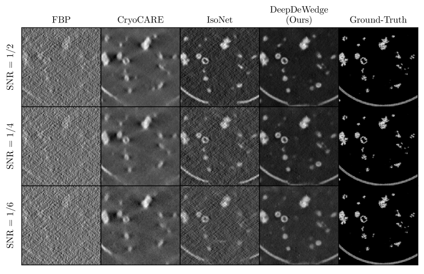
Figure 6: Visual comparison between CryoCARE, IsoNet, and our method (with even/odd split) on a tomogram from the synthetic dataset. The images are crops of slices through the tomograms along the plane that is perpendicular to the optical axis. In such slices, the missing wedge artifacts are most prominent.

3 Discussion

In this paper, we have proposed DeepDeWedge, which is a new deep-learning-based method for denoising and missing wedge reconstruction in cryo-ET. Our method achieves significantly improved denoising performance compared to its closest competitor, IsoNet. Even when only considering the part without the missing edge, our method is on par with that of state-of-the-art noise2noise-like denoising methods such as cryoCARE, which do not perform missing wedge reconstruction.

In addition, by taking a noise2noise-inspired denoising approach, our method makes fewer assumptions on the noise than IsoNet and, as a consequence, has fewer hyperparameters and thus is simpler to use. We found the missing wedge-filling ability of our method to be on par with that of IsoNet.

It is important to keep in mind that the missing wedge is irreversibly lost during tilt series acquisition. Therefore, the data filled in for it by our method is not based on actual measurements of the missing wedge data itself. Instead, the network used in our approach learns to fill in the missing wedge by predicting data that we artificially removed. This process is exclusively based on measurement data and uses no priors or assumptions on the sample. Still, it is an open question to what degree the predicted missing wedge can be trusted, and we advise users of our method to be cautious.

Based on these considerations, we see two main applications for our method: First, it is an easy way to improve the direct interpretability of tomograms for humans, which facilitates deciding on steps for further analysis. Second, tomograms reconstructed with our method can be used as input for downstream tasks such as particle picking. It has already been observed that denoised and/or missing-wedge-corrected tomograms can improve the performance of deep-learning-based particle pickers [Buc+19, Liu+22, Hon+23]. For subsequent steps, such as sub-tomogram averaging, one can then use the original raw tomograms that are not modified by the neural network.

Data Availability

The EMPIAR-10045 dataset used for the experiments discussed in Section 2.2.1 is publicly available through EMPIAR. We downloaded it from this website: https://www.ebi.ac.uk/empiar/EMPIAR-10045/. The tutorial dataset of CryoCARE is publicly available via GitHub https://github.com/juglab/cryoCARE_T2T, through the following download link: https://download.fht.org/jug/cryoCARE/Tomo110.zip. The synthetic dataset by [Gub+20] is also publicly available and can be downloaded from this website: https://dataverse.nl/dataset.xhtml?persistentId=doi:10.34894/XRTJMA.

Code Availability

We provide an implementation of DeepDeWedge on GitHub: https://github.com/MLI-lab/DeepDeWedge.

Appendix A Background on Self-Supervised Deep Learning Techniques

The DeepDeWedge loss is inspired by noise2noise and noisier2noise self-supervised learning. Here, we give a brief overview of the main ideas behind these two frameworks.

A.1 Denoising with Noise2Noise

Noise2noise is a framework for constructing a loss function that enables training a neural network for image denoising without ground-truth images. Neural networks for denoising are typically trained in a supervised fashion to map a noisy image to a clean one and thus require pairs of clean images and corresponding measurements.

Noise2noise-based methods also aim to train a neural network to map a noisy image to a clean one. Contrary to supervised learning, noise2noise assumes access to a dataset of pairs of noisy observations ${\color[rgb]{1,0,0}\mathbf{y}^{0}_{i}}=\mathbf{x}^{*}_{i}+{\color[rgb]{1,0,0}\mathbf{n}^{0}_{i}}$ and ${\color[rgb]{0,0,1}\mathbf{y}^{1}_{i}}=\mathbf{x}^{*}_{i}+{\color[rgb]{0,0,1}\mathbf{n}^{1}_{i}}$ for each ground-truth image $\mathbf{x}^{*}_{i}$. Moreover, it assumes that the noise terms ${\color[rgb]{1,0,0}\mathbf{n}^{0}_{i}}$ and ${\color[rgb]{0,0,1}\mathbf{n}^{1}_{i}}$ are independent and that the noise ${\color[rgb]{0,0,1}\mathbf{n}^{1}_{i}}$ is zero-mean. Then, one can train a network $f_{\text{$\boldsymbol{\theta}$}}$ for denoising to map the noisy observation ${\color[rgb]{1,0,0}\mathbf{y}^{0}}$ onto its counterpart ${\color[rgb]{0,0,1}\mathbf{y}^{1}}$. Formally, one can show that

$$\mathop{\mathbb{E}}_{{\color[rgb]{1,0,0}\mathbf{y}^{0}},{\color[rgb]{0,0,1}\mathbf{y}^{1}}}\Big{[}\left|\left|f_{\text{$\boldsymbol{\theta}$}}({\color[rgb]{1,0,0}\mathbf{y}^{0}})-{\color[rgb]{0,0,1}\mathbf{y}^{1}}\right|\right|_{2}^{2}\Big{]}=\mathop{\mathbb{E}}_{{\color[rgb]{1,0,0}\mathbf{y}^{0}},\mathbf{x}^{*}}\Big{[}\left|\left|f_{\text{$\boldsymbol{\theta}$}}({\color[rgb]{1,0,0}\mathbf{y}^{0}})-\mathbf{x}^{*}\right|\right|_{2}^{2}\Big{]}+c,$$ (7)

where $c$ is a constant that is independent of the network weights $\boldsymbol{\theta}$. Thus, a self-supervised noise2noise training objective based on samples approximates, up to an additive constant, the same underlying risk (left side of Equation (7)) as the supervised objective function. This approximation becomes better as the number of training examples increases and theoretically and empirically, networks trained with a noise2noise-like loss perform as well as if trained on sufficiently many examples [KAH23].

A.2 Denoising and Recovering Missing Data with Noiser2Noise

IsoNet’s denoising approach is motivated by the noisier2noise framework [Mor+20]. While training a model for image denoising with a noise2noise objective requires paired noisy observations, a noisier2noise objective is based on a single noisy observation per image.

Noisier2Noise for Denoising: We assume that we have access to a dataset of noisy images. Contrary to noise2noise, we assume that we have only one single noisy observation $\mathbf{y}=\mathbf{x}^{*}+\mathbf{n}$ per ground-truth $\mathbf{x}^{*}$. The goal is to train a neural network for image denoising. For constructing a training objective with noisier2noise, we assume that the noise terms $\mathbf{n}$ that corrupt all images come from the same distribution and that we are able to sample from this distribution. We construct model inputs $\tilde{\mathbf{y}}$ by further corrupting the noisy images $\mathbf{y}$ with an additional noise term $\tilde{\mathbf{n}}$ sampled from the true noise distribution, i.e., $\tilde{\mathbf{y}}=\mathbf{y}+\tilde{\mathbf{n}}$. [Mor+20] showed that if we train a neural network $f_{\text{$\boldsymbol{\theta}$}}$ to map these noisier model inputs $\tilde{\mathbf{y}}$ onto their single noisy counterparts $\mathbf{y}$ using the squared L2-loss, one can use the final trained network to construct a denoiser for the double noisy images $\tilde{\mathbf{y}}$.

Noisier2Noise for Missing Data Recovery: We use ideas from noisier2noise for missing wedge reconstruction. To illustrate how noisier2noise can be used to predict missing data, consider the following setup: Assume we have a dataset of masked measurements $\mathbf{y}=\mathbf{M}\mathbf{x}^{*}$. Here, $\mathbf{M}$ denotes a random mask, i.e., a diagonal matrix with entries in $\{0,1\}$, and $\mathbf{x}^{*}$ is an unknown ground-truth signal vector. Like above, the ground truths and masks are different for each measurement $\mathbf{y}$ and the dataset contains only the measurements and no ground truths. In this setup, we want to train a neural network $f_{\text{$\boldsymbol{\theta}$}}$ to predict the data $\mathbf{x}^{*}$ from the measurement $\mathbf{y}$. To do this, we construct double-masked measurements $\tilde{\mathbf{y}}=\mathbf{{\color[rgb]{0,0,0}\tilde{M}}}\mathbf{y}$, where $\mathbf{{\color[rgb]{0,0,0}\tilde{M}}}$ is another random mask, and train the network to map the double-masked measurements $\tilde{\mathbf{y}}$ to their counterparts $\mathbf{y}$. It can be shown that, under certain assumptions on the random masks $\mathbf{M}$ and $\mathbf{{\color[rgb]{0,0,0}\tilde{M}}}$, the final trained model can be used in an algorithm to recover the data missing in the singly masked measurements $\mathbf{y}$. As for denoising, the model estimates the missing data based on the doubly-masked measurement $\tilde{\mathbf{y}}$. For details, we refer readers to recent works by [MC23][MC23, MC22], who discussed noisier2noise for the recovery of missing data in accelerated magnetic resonance imaging.

Appendix B Proof of Proposition 1

We divide the proof of Proposition 1 into two steps. The first step, which we present as a lemma, is a result inspired by noise2noise and deals with the additive noise ${\color[rgb]{0,0,1}\mathbf{n}^{\text{1}}}$ on the model target. To facilitate notation, we assume from now on that all 3D objects are represented as column vectors in $\mathbb{R}^{n}$ for $n=N^{3}$, and that the masks $\mathbf{M}$ and $\mathbf{{\color[rgb]{0,0,0}\tilde{M}}}$ are random diagonal matrices with entries in $\{0,1\}$.

Lemma 1.

Assume that the noise term ${\color[rgb]{0,0,1}\mathbf{n}^{\text{1}}}$ is zero-mean and independent of the noise term ${\color[rgb]{1,0,0}\mathbf{n}^{\text{0}}}$ and the masks $\mathbf{M}$ and $\mathbf{{\color[rgb]{0,0,0}\tilde{M}}}$. Then

$$\mathop{\mathbb{E}}_{{\color[rgb]{0,0,1}\mathbf{n}^{\text{1}}}}\Bigg{[}\left|\left|\big{(}\mathbf{{\color[rgb]{0,0,0}\tilde{M}}}\mathbf{M}+2\mathbf{{\color[rgb]{0,0,0}\tilde{M}}}^{C}\mathbf{M}\big{)}\mathbf{F}\Big{(}f_{\text{$\boldsymbol{\theta}$}}\big{(}{\color[rgb]{1,0,0}\tilde{\mathbf{v}}_{{\color[rgb]{0,0,0}}}^{\text{0}}}\big{)}-{\color[rgb]{0,0,1}\mathbf{v}_{{\color[rgb]{0,0,0}}}^{\text{1}}}\Big{)}\right|\right|_{2}^{2}\Bigg{]}=\left|\left|\big{(}\mathbf{{\color[rgb]{0,0,0}\tilde{M}}}\mathbf{M}+2\mathbf{{\color[rgb]{0,0,0}\tilde{M}}}^{C}\mathbf{M}\big{)}\mathbf{F}\Big{(}f_{\text{$\boldsymbol{\theta}$}}({\color[rgb]{1,0,0}\tilde{\mathbf{v}}_{{\color[rgb]{0,0,0}}}^{\text{0}}})-\mathbf{v}^{*}\Big{)}\right|\right|_{2}^{2}+c_{,}$$

where $c>0$ is a constant that does not depend on the weights $\boldsymbol{\theta}$.

Proof of Lemma 1.

We calculate

$$\left|\left|\mathbf{{\color[rgb]{0,0,0}\tilde{M}}}\mathbf{M}\mathbf{F}\big{(}f_{\text{$\boldsymbol{\theta}$}}({\color[rgb]{1,0,0}\tilde{\mathbf{v}}_{{\color[rgb]{0,0,0}}}^{\text{0}}})-{\color[rgb]{0,0,1}\mathbf{v}_{{\color[rgb]{0,0,0}}}^{\text{1}}}\big{)}\right|\right|_{2}^{2} =\left|\left|\mathbf{{\color[rgb]{0,0,0}\tilde{M}}}\mathbf{M}\mathbf{F}\big{(}f_{\text{$\boldsymbol{\theta}$}}({\color[rgb]{1,0,0}\tilde{\mathbf{v}}_{{\color[rgb]{0,0,0}}}^{\text{0}}})-\mathbf{F}^{-1}\mathbf{M}\mathbf{F}\big{(}\mathbf{v}^{*}+{\color[rgb]{0,0,1}\mathbf{n}^{\text{1}}}\big{)}\big{)}\right|\right|_{2}^{2}$$

$$=\left|\left|\mathbf{{\color[rgb]{0,0,0}\tilde{M}}}\mathbf{M}\mathbf{F}\big{(}f_{\text{$\boldsymbol{\theta}$}}({\color[rgb]{1,0,0}\tilde{\mathbf{v}}_{{\color[rgb]{0,0,0}}}^{\text{0}}})-\big{(}\mathbf{v}^{*}+{\color[rgb]{0,0,1}\mathbf{n}^{\text{1}}}\big{)}\big{)}\right|\right|_{2}^{2},$$

$$=\left|\left|\mathbf{{\color[rgb]{0,0,0}\tilde{M}}}\mathbf{M}\mathbf{F}\big{(}f_{\text{$\boldsymbol{\theta}$}}({\color[rgb]{1,0,0}\tilde{\mathbf{v}}_{{\color[rgb]{0,0,0}}}^{\text{0}}})-\mathbf{v}^{*}\big{)}\right|\right|_{2}^{2}$$

$$\qquad-2\left\langle\mathbf{{\color[rgb]{0,0,0}\tilde{M}}}\mathbf{M}\mathbf{F}\big{(}f_{\text{$\boldsymbol{\theta}$}}({\color[rgb]{1,0,0}\tilde{\mathbf{v}}_{{\color[rgb]{0,0,0}}}^{\text{0}}})-\mathbf{v}^{*}\big{)},\mathbf{{\color[rgb]{0,0,0}\tilde{M}}}\mathbf{M}\mathbf{F}{\color[rgb]{0,0,1}\mathbf{n}^{\text{1}}}\right\rangle$$

$$\qquad+\left|\left|\mathbf{{\color[rgb]{0,0,0}\tilde{M}}}\mathbf{M}\mathbf{F}{\color[rgb]{0,0,1}\mathbf{n}^{\text{1}}}\right|\right|_{2}^{2},$$

where we used in the second step that $\mathbf{M}^{2}=\mathbf{M}$, as $\mathbf{M}$ is a diagonal matrix with entries in $\{0,1\}$. As we assumed the noise ${\color[rgb]{0,0,1}\mathbf{n}^{\text{1}}}$ to be zero-mean and independent of the noise ${\color[rgb]{1,0,0}\mathbf{n}^{\text{0}}}$, and the masks $\mathbf{M}$ and $\mathbf{{\color[rgb]{0,0,0}\tilde{M}}}$, it holds that

$$\mathop{\mathbb{E}}_{{\color[rgb]{0,0,1}\mathbf{n}^{\text{1}}}}\Bigg{[}\left\langle\mathbf{{\color[rgb]{0,0,0}\tilde{M}}}\mathbf{M}\mathbf{F}\big{(}f_{\text{$\boldsymbol{\theta}$}}({\color[rgb]{1,0,0}\tilde{\mathbf{v}}_{{\color[rgb]{0,0,0}}}^{\text{0}}})-\mathbf{v}^{*}\big{)},\mathbf{{\color[rgb]{0,0,0}\tilde{M}}}\mathbf{M}\mathbf{F}{\color[rgb]{0,0,1}\mathbf{n}^{\text{1}}}\right\rangle\Bigg{]}=0.$$

Therefore we get

$$\mathop{\mathbb{E}}_{{\color[rgb]{0,0,1}\mathbf{n}^{\text{1}}}}\Bigg{[}\left|\left|\mathbf{{\color[rgb]{0,0,0}\tilde{M}}}\mathbf{M}\mathbf{F}\big{(}f_{\text{$\boldsymbol{\theta}$}}({\color[rgb]{1,0,0}\tilde{\mathbf{v}}_{{\color[rgb]{0,0,0}}}^{\text{0}}})-{\color[rgb]{0,0,1}\mathbf{v}_{{\color[rgb]{0,0,0}}}^{\text{1}}}\big{)}\right|\right|_{2}^{2}\Bigg{]}=\left|\left|\mathbf{{\color[rgb]{0,0,0}\tilde{M}}}\mathbf{M}\mathbf{F}\big{(}f_{\text{$\boldsymbol{\theta}$}}({\color[rgb]{1,0,0}\tilde{\mathbf{v}}_{{\color[rgb]{0,0,0}}}^{\text{0}}})-\mathbf{v}^{*}\big{)}\right|\right|_{2}^{2}+\mathop{\mathbb{E}}_{{\color[rgb]{0,0,1}\mathbf{n}^{\text{1}}}}\Bigg{[}\left|\left|\mathbf{{\color[rgb]{0,0,0}\tilde{M}}}\mathbf{M}\mathbf{F}{\color[rgb]{0,0,1}\mathbf{n}^{\text{1}}}\right|\right|_{2}^{2}\Bigg{]}.$$

An analogous argument yields

$$\mathop{\mathbb{E}}_{{\color[rgb]{0,0,1}\mathbf{n}^{\text{1}}}}\Bigg{[}\left|\left|\mathbf{{\color[rgb]{0,0,0}\tilde{M}}}^{C}\mathbf{M}\mathbf{F}\big{(}f_{\text{$\boldsymbol{\theta}$}}({\color[rgb]{1,0,0}\tilde{\mathbf{v}}_{{\color[rgb]{0,0,0}}}^{\text{0}}})-{\color[rgb]{0,0,1}\mathbf{v}_{{\color[rgb]{0,0,0}}}^{\text{1}}}\big{)}\right|\right|_{2}^{2}\Bigg{]}=\left|\left|\mathbf{{\color[rgb]{0,0,0}\tilde{M}}}^{C}\mathbf{M}\mathbf{F}\big{(}f_{\text{$\boldsymbol{\theta}$}}({\color[rgb]{1,0,0}\tilde{\mathbf{v}}_{{\color[rgb]{0,0,0}}}^{\text{0}}})-\mathbf{v}^{*}\big{)}\right|\right|_{2}^{2}+\mathop{\mathbb{E}}_{{\color[rgb]{0,0,1}\mathbf{n}^{\text{1}}}}\Bigg{[}\left|\left|\mathbf{{\color[rgb]{0,0,0}\tilde{M}}}^{C}\mathbf{M}\mathbf{F}{\color[rgb]{0,0,1}\mathbf{n}^{\text{1}}}\right|\right|_{2}^{2}\Bigg{]}.$$

Using the fact that the joint masks $\mathbf{{\color[rgb]{0,0,0}\tilde{M}}}\mathbf{M}$ and $\mathbf{{\color[rgb]{0,0,0}\tilde{M}}}^{C}\mathbf{M}$ are orthogonal to each other and setting

$$c=\mathop{\mathbb{E}}_{\mathbf{M},\mathbf{{\color[rgb]{0,0,0}\tilde{M}}},{\color[rgb]{0,0,1}\mathbf{n}^{\text{1}}}}\Bigg{[}\left|\left|\big{(}\mathbf{{\color[rgb]{0,0,0}\tilde{M}}}\mathbf{M}+2\mathbf{{\color[rgb]{0,0,0}\tilde{M}}}^{C}\mathbf{M}\big{)}\mathbf{F}{\color[rgb]{0,0,1}\mathbf{n}^{\text{1}}}\right|\right|_{2}^{2}\Bigg{]},$$

yields the desired result. ∎

Proof of Proposition 1.

For the sake of generality, we omit the assumption that the missing wedge masks $\mathbf{M}$ and $\mathbf{{\color[rgb]{0,0,0}\tilde{M}}}$ are non-overlapping and show that

$$\mathop{\mathbb{E}}_{\mathbf{M},\mathbf{{\color[rgb]{0,0,0}\tilde{M}}},{\color[rgb]{1,0,0}\mathbf{n}^{\text{0}}},{\color[rgb]{0,0,1}\mathbf{n}^{\text{1}}}}\Bigg{[}\left|\left|\big{(}\mathbf{{\color[rgb]{0,0,0}\tilde{M}}}\mathbf{M}+2\mathbf{{\color[rgb]{0,0,0}\tilde{M}}}^{C}\mathbf{M}\big{)}\mathbf{F}\Big{(}f_{\text{$\boldsymbol{\theta}$}}({\color[rgb]{1,0,0}\tilde{\mathbf{v}}_{{\color[rgb]{0,0,0}}}^{\text{0}}})-{\color[rgb]{0,0,1}\mathbf{v}_{{\color[rgb]{0,0,0}}}^{\text{1}}}\Big{)}\right|\right|_{2}^{2}\Bigg{]}=\mathop{\mathbb{E}}_{\mathbf{M},\mathbf{{\color[rgb]{0,0,0}\tilde{M}}},{\color[rgb]{1,0,0}\mathbf{n}^{\text{0}}}}\Bigg{[}\left|\left|\big{(}\mathbf{I}-\mathbf{{\color[rgb]{0,0,0}\tilde{M}}}^{C}\mathbf{M}^{C}\big{)}\mathbf{F}\big{(}f_{\text{$\boldsymbol{\theta}$}}({\color[rgb]{1,0,0}\tilde{\mathbf{v}}_{{\color[rgb]{0,0,0}}}^{\text{0}}})-\mathbf{v}^{*}\big{)}\right|\right|_{2}^{2}\Bigg{]}+c,$$ (8)

where $c$ is the constant from Lemma 1. Here, the mask $\mathbf{I}-\mathbf{{\color[rgb]{0,0,0}\tilde{M}}}^{C}\mathbf{M}^{C}$ zeros out all Fourier components that are contained in both missing wedges. If the wedges are non-overlapping, this joint mask reduces to the identity $\mathbf{I}$, and we obtain the result stated in Proposition 1.

By Lemma 1, in order to show Equation (8), it suffices to show that

$$\mathop{\mathbb{E}}_{\mathbf{M},\mathbf{{\color[rgb]{0,0,0}\tilde{M}}},{\color[rgb]{1,0,0}\mathbf{n}^{\text{0}}}}\Bigg{[}\left|\left|\big{(}\mathbf{{\color[rgb]{0,0,0}\tilde{M}}}\mathbf{M}+2\mathbf{{\color[rgb]{0,0,0}\tilde{M}}}^{C}\mathbf{M}\big{)}\mathbf{F}\Big{(}f_{\text{$\boldsymbol{\theta}$}}({\color[rgb]{1,0,0}\tilde{\mathbf{v}}_{{\color[rgb]{0,0,0}}}^{\text{0}}})-\mathbf{v}^{*}\Big{)}\right|\right|_{2}^{2}\Bigg{]}=\mathop{\mathbb{E}}_{\mathbf{M},\mathbf{{\color[rgb]{0,0,0}\tilde{M}}},{\color[rgb]{1,0,0}\mathbf{n}^{\text{0}}}}\Bigg{[}\left|\left|\big{(}\mathbf{I}-\mathbf{{\color[rgb]{0,0,0}\tilde{M}}}^{C}\mathbf{M}^{C}\big{)}\mathbf{F}\big{(}f_{\text{$\boldsymbol{\theta}$}}({\color[rgb]{1,0,0}\tilde{\mathbf{v}}_{{\color[rgb]{0,0,0}}}^{\text{0}}})-\mathbf{v}^{*}\big{)}\right|\right|_{2}^{2}\Bigg{]}.$$ (9)

Now we analyze the left-hand side of this equation. We fix the noise ${\color[rgb]{1,0,0}\mathbf{n}^{\text{0}}}$ and calculate

$$\mathop{\mathbb{E}}_{\mathbf{M},\mathbf{{\color[rgb]{0,0,0}\tilde{M}}}}\left[\left|\left|2\mathbf{{\color[rgb]{0,0,0}\tilde{M}}}^{C}\mathbf{M}\mathbf{F}\big{(}f_{\text{$\boldsymbol{\theta}$}}({\color[rgb]{1,0,0}\tilde{\mathbf{v}}_{{\color[rgb]{0,0,0}}}^{\text{0}}})-\mathbf{v}^{*}\big{)}\right|\right|_{2}^{2}\right]$$

$$=\mathop{\mathbb{E}}_{\mathbf{M},\mathbf{{\color[rgb]{0,0,0}\tilde{M}}}}\left[\left|\left|\mathbf{{\color[rgb]{0,0,0}\tilde{M}}}^{C}\mathbf{M}\mathbf{F}\big{(}f_{\text{$\boldsymbol{\theta}$}}({\color[rgb]{1,0,0}\tilde{\mathbf{v}}_{{\color[rgb]{0,0,0}}}^{\text{0}}})-\mathbf{v}^{*}\big{)}\right|\right|_{2}^{2}\right]+\mathop{\mathbb{E}}_{\mathbf{M},\mathbf{{\color[rgb]{0,0,0}\tilde{M}}}}\left[\left|\left|\mathbf{{\color[rgb]{0,0,0}\tilde{M}}}^{C}\mathbf{M}\mathbf{F}\big{(}f_{\text{$\boldsymbol{\theta}$}}({\color[rgb]{1,0,0}\tilde{\mathbf{v}}_{{\color[rgb]{0,0,0}}}^{\text{0}}})-\mathbf{v}^{*}\big{)}\right|\right|_{2}^{2}\right]$$

$$=\mathop{\mathbb{E}}_{\mathbf{M},\mathbf{{\color[rgb]{0,0,0}\tilde{M}}}}\left[\left|\left|\mathbf{{\color[rgb]{0,0,0}\tilde{M}}}^{C}\mathbf{M}\mathbf{F}\big{(}f_{\text{$\boldsymbol{\theta}$}}({\color[rgb]{1,0,0}\tilde{\mathbf{v}}_{{\color[rgb]{0,0,0}}}^{\text{0}}})-\mathbf{v}^{*}\big{)}\right|\right|_{2}^{2}\right]+\mathop{\mathbb{E}}_{\mathbf{M},\mathbf{{\color[rgb]{0,0,0}\tilde{M}}}}\left[\left|\left|\mathbf{M}^{C}\mathbf{{\color[rgb]{0,0,0}\tilde{M}}}\mathbf{F}\big{(}f_{\text{$\boldsymbol{\theta}$}}({\color[rgb]{1,0,0}\tilde{\mathbf{v}}_{{\color[rgb]{0,0,0}}}^{\text{0}}})-\mathbf{v}^{*}\big{)}\right|\right|_{2}^{2}\right]$$

$$=\mathop{\mathbb{E}}_{\mathbf{M},\mathbf{{\color[rgb]{0,0,0}\tilde{M}}}}\left[\left|\left|(\mathbf{{\color[rgb]{0,0,0}\tilde{M}}}^{C}\mathbf{M}+\mathbf{M}^{C}\mathbf{{\color[rgb]{0,0,0}\tilde{M}}})\mathbf{F}\big{(}f_{\text{$\boldsymbol{\theta}$}}({\color[rgb]{1,0,0}\tilde{\mathbf{v}}_{{\color[rgb]{0,0,0}}}^{\text{0}}})-\mathbf{v}^{*}\big{)}\right|\right|_{2}^{2}\right].$$

For the second equation, we used that $P(\mathbf{M},\mathbf{{\color[rgb]{0,0,0}\tilde{M}}})=P(\mathbf{{\color[rgb]{0,0,0}\tilde{M}}},\mathbf{M})$ and that the model input ${\color[rgb]{1,0,0}\tilde{\mathbf{v}}_{{\color[rgb]{0,0,0}}}^{\text{0}}}$ depends on the masks $\mathbf{M}$ and $\mathbf{{\color[rgb]{0,0,0}\tilde{M}}}$ only through their product $\mathbf{M}\mathbf{{\color[rgb]{0,0,0}\tilde{M}}}$, for which the order of the masks does not play a role, thus the role of the two masks is exchangeable. For the last equation, we used that the masks $\mathbf{{\color[rgb]{0,0,0}\tilde{M}}}^{C}\mathbf{M}$ and $\mathbf{M}^{C}\mathbf{{\color[rgb]{0,0,0}\tilde{M}}}$ are orthogonal.

Using this equation and the fact that $\mathbf{{\color[rgb]{0,0,0}\tilde{M}}}\mathbf{M}$, $\mathbf{{\color[rgb]{0,0,0}\tilde{M}}}^{C}\mathbf{M}$ and $\mathbf{M}^{C}\mathbf{{\color[rgb]{0,0,0}\tilde{M}}}$ are orthogonal to each other, the left-hand side of Equation 9 becomes

$$\mathop{\mathbb{E}}_{\mathbf{M},\mathbf{{\color[rgb]{0,0,0}\tilde{M}}},{\color[rgb]{1,0,0}\mathbf{n}^{\text{0}}}}\Bigg{[}\left|\left|\big{(}\mathbf{{\color[rgb]{0,0,0}\tilde{M}}}\mathbf{M}+\mathbf{{\color[rgb]{0,0,0}\tilde{M}}}^{C}\mathbf{M}+\mathbf{M}^{C}\mathbf{{\color[rgb]{0,0,0}\tilde{M}}}\big{)}\mathbf{F}\big{(}f_{\text{$\boldsymbol{\theta}$}}({\color[rgb]{1,0,0}\tilde{\mathbf{v}}_{{\color[rgb]{0,0,0}}}^{\text{0}}})-\mathbf{v}^{*}\big{)}\right|\right|_{2}^{2}\Bigg{]}\stackrel{{\scriptstyle(*)}}{{=}}\mathop{\mathbb{E}}_{\mathbf{M},\mathbf{{\color[rgb]{0,0,0}\tilde{M}}},{\color[rgb]{1,0,0}\mathbf{n}^{\text{0}}}}\Bigg{[}\left|\left|\big{(}\mathbf{I}-\mathbf{{\color[rgb]{0,0,0}\tilde{M}}}^{C}\mathbf{M}^{C}\big{)}\mathbf{F}\big{(}f_{\text{$\boldsymbol{\theta}$}}({\color[rgb]{1,0,0}\tilde{\mathbf{v}}_{{\color[rgb]{0,0,0}}}^{\text{0}}})-\mathbf{v}^{*}\big{)}\right|\right|_{2}^{2}\Bigg{]},$$

where the equality $(*)$ holds because

$$\mathbf{{\color[rgb]{0,0,0}\tilde{M}}}\mathbf{M}+\mathbf{{\color[rgb]{0,0,0}\tilde{M}}}^{C}\mathbf{M}+\mathbf{M}^{C}\mathbf{{\color[rgb]{0,0,0}\tilde{M}}} =\mathbf{{\color[rgb]{0,0,0}\tilde{M}}}\mathbf{M}+(\mathbf{I}-\mathbf{{\color[rgb]{0,0,0}\tilde{M}}})\mathbf{M}+(\mathbf{I}-\mathbf{M})\mathbf{{\color[rgb]{0,0,0}\tilde{M}}}$$

$$=\mathbf{{\color[rgb]{0,0,0}\tilde{M}}}\mathbf{M}+\mathbf{M}-\mathbf{{\color[rgb]{0,0,0}\tilde{M}}}\mathbf{M}+\mathbf{{\color[rgb]{0,0,0}\tilde{M}}}-\mathbf{M}\mathbf{{\color[rgb]{0,0,0}\tilde{M}}}$$

$$=\mathbf{M}-\mathbf{{\color[rgb]{0,0,0}\tilde{M}}}\mathbf{M}+\mathbf{{\color[rgb]{0,0,0}\tilde{M}}}$$

$$=\mathbf{I}-(\mathbf{I}-\mathbf{{\color[rgb]{0,0,0}\tilde{M}}})(\mathbf{I}-\mathbf{M})$$

$$=\mathbf{I}-\mathbf{{\color[rgb]{0,0,0}\tilde{M}}}^{C}\mathbf{M}^{C}.$$

This concludes the proof of Equation 9 and Proposition 1.

∎

Appendix C Details on Experiments

Here, we provide additional technical details of our experiments discussed in Section 2.2. For all experiments, we used the Adam optimizer [KB15] with a constant learning rate of $4\cdot 10^{-4}$. The remaining details are as follows:

C.1 Details on Section 2.2.1

• FBP and sub-tomograms: We performed all FBP reconstructions with a ramp filter in Python using the library tomosipo [Hen+21]. After reconstruction, we downsampled all tomograms by a factor of 6 using average pooling, which resulted in a final voxel size of 13.02 Å. To these tomograms, we applied IsoNet’s CTF deconvolution routine with parameters as described by [Liu+22] in their paper. For model fitting, we extracted sub-tomograms of shape $80\times 80\times 80$. As wide regions of the tomograms contain only ice and no ribosomes, we used the make mask routine implemented in IsoNet to generate a mask of the non-empty regions. After extracting the sub-tomograms, we selected only those that contain at least 40% sample according to the mask, which resulted in around 420 sub-tomograms for model fitting. For the refinement with the fitted model, we also used sub-tomograms of shape $80\times 80\times 80$ voxels, but extracted them without masking and with an overlap of 40 voxels.

• Details on IsoNet: We fitted IsoNet for 45 iterations with 10 epochs per iteration and a batch size of 10. We used the default noise schedule for fitting, which starts adding noise with level 0.05 in iteration 11 and then increases the noise level by 0.05 every 5 iterations. We set the noise_mode parameter, which determines the distribution of the additional noise used for noisier2noise-like denoising, to noFilter, which corresponds to Gaussian noise. We also tried setting the noise mode to ramp, as the tomograms were reconstructed with FBP with a ramp filter, but this gave worse results. In their paper, [Liu+22] fitted IsoNet for 30 iterations using similarly many sub-tomograms and the same number of epochs. However, we found that 45 iterations gave visually more appealing results compared to the images shown in the IsoNet paper.

• Details on our DeepDeWedge: To be consistent with IsoNet’s fitting time, we fitted the model for 450 epochs. Although the loss on a holdout validation set was still decreasing after that point, we found that the appearance of the reconstructions themselves did not change much anymore.

C.2 Details on Section 2.2.2

• FBP and sub-tomograms: We followed the steps described in the CryoCARE GitHub repository (https://github.com/juglab/cryoCARE_T2T/tree/master/example) to reconstruct a tomogram from the tilt series with IMOD [KMM96]. We downsampled the tomogram by a factor of 6 using average pooling, which resulted in a voxel size of $14.13$ Å. As IsoNet is optimized for a missing wedge of $60^{\circ}$, we artificially widened the missing wedge from the original $50^{\circ}$ to $60^{\circ}$ by multiplying the reconstruction with a missing wedge filter in the Fourier domain for a fair comparison. Finally, we extracted around 150 sub-tomograms with shape $96\times 96\times 96$ for model fitting. For the final refinement after model fitting, we used the same sub-tomogram size extracted with an overlap of 32 voxels.

• Details on IsoNet: We fitted IsoNet for 60 iterations with 20 epochs per iteration and a batch size of 5. Again, we used the default noise schedule and set the noise mode to noFilter as described above. After fitting, we evaluated the IsoNet models every 5 iterations and chose the one that gave the visually most appealing reconstruction. For Wiener-filter-based CTF correction, this occurred in iteration 45. For phase flipping, the reconstruction from iteration 30 looked best.

• Details on DeepDeWedge: We fitted the model for 1000 epochs. Although the loss on the validation set was still decreasing, the reconstructions did not change much anymore.

C.3 Details on Section 2.2.3

• FBP and sub-tomograms: We performed FBP using tomosipo, this time with a Hamming-like filter (see below). We fitted all models model using sub-tomograms of size $96\times 96\times 96$. To refine the FBP reconstructions after model fitting, we applied the final fitted networks to sub-tomograms of the same size, using an overlap of 32 voxels.

• Details on CryoCARE: Despite the use of dropout, we observed overfitting, so we applied early stopping on a subset of the ground truth data to get an impression of the best-case performance. To obtain the final denoised tomograms, we followed the approach proposed by Buchholz et al. [Buc+19] of applying the trained model to the even and odd FBP reconstructions independently and then averaging both tomograms instead of applying the model to the FBP reconstruction of the full tilt series as for our method.

• Details on IsoNet: As our simulated dataset does not contain CTF effects, we did not perform the CTF deconvolution preprocessing step, which is usually performed to increase the contrast of the FBP reconstructions and improve IsoNet’s performance. We compensated for this by using the Hamming-like filter for FBP, which improves the contrast compared to the standard ramp filter. We fitted IsoNet for 50 iterations with 20 epochs per iteration. We again followed the default noise schedule described above and set the noise mode to hamming.

  As there is no principled way to determine when to stop IsoNet fitting or how much noise to add, we did the following to obtain a very strong baseline: We evaluated the IsoNet reconstructions after every iteration using all comparison metrics and chose the best result for each metric, which yields best-case performance. We emphasize that this approach is not possible in practice where ground truth is not available. The optimal performance of each model occurred for every SNR between iterations 30 and 40, i.e., between 600 and 800 epochs.

• Details on DeepDeWedge: To keep the computational cost between IsoNet and our method comparable, we fitted the network for exactly 600 epochs in our approach.

Appendix D Ablations

In this section, we investigate the impact of several hyperparameters on the performance of our method. If not explicitly stated otherwise, we fitted all models on simulated tilt series from the first 3 tomograms of the Dataset by [Gub+20] with SNR $1/4$. We performed only one run for each experiment. All remaining details regarding the model and optimizer are as described in Section 2.2.3 and Appendix C.

D.1 Influence of Sub-Tomogram Size on Performance

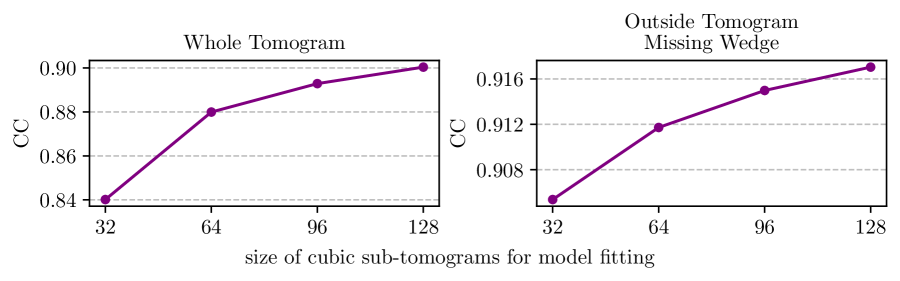
Figure 7: Performance metrics for different sub-tomogram sizes used for model fitting.

The size of the sub-tomograms used for model fitting is a hyperparameter of DeepDeWedge, and here we investigate how it affects the performance. To this end, we repeated the experiment on synthetic data described in Section 2.2.3 for increasing the size of sub-tomograms. We scaled the total number of sub-tomograms for each run such that the number of voxels of the sub-tomogram fitting dataset is approximately constant. As for model fitting, we have to rotate the sub-tomograms, the sub-tomograms we extract have to be larger than the ones we actually use for fitting in order to avoid having to use padding. As a result, the maximum sub-tomogram size we could use for model fitting is $128\times 128\times 128$.

We fitted all models for 1500 epochs. During fitting, we evaluated the models on all three tilt series every 100 epochs and report the highest SNRs, to get an impression of the best-case performance. As this procedure is computationally very expensive, we did not calculate the per-particle FSC metrics.

Figure 7 suggests that larger sub-tomograms for model fitting yield better performance than smaller ones.

D.2 Tilt-Series Splitting

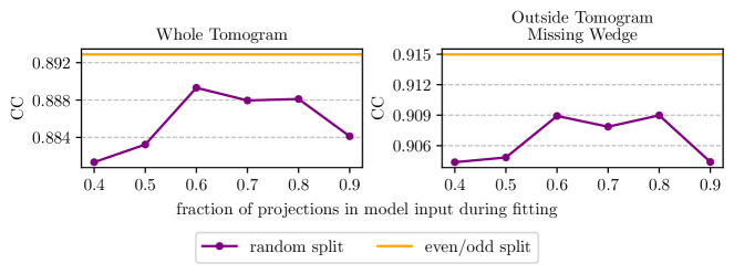
Figure 8: Performance metrics for different fractions of tilt series images used to construct the model inputs.

In the main body, we discussed two approaches for splitting a tilt series into two sub-tilt series, which are then used to construct the model inputs and targets: the even/odd split and a frame-based method. Here, we investigate another splitting method, which consists of randomly selecting a given fraction of tilt series projections to construct the model inputs and using the remaining ones for the targets. Again, we fitted each model for 1500 epochs and used the same approach for model selection as described above in Appendix D.1.

Figure 8 shows the result of our comparison. Overall, all splitting fractions for the random splitting approach yield similar performance and are slightly outperformed by the even/odd split.

D.3 Applying DeepDeWedge to Multiple Tilt Series Simultaneously

As stated in the main body, and as done in some of our experiments in Section 2.2, DeepDeWedge can be applied to multiple tilt series from similar samples simultaneously. Here, we discuss how this impacts performance compared to applying DeepDeWedge to each tilt series separately. We compare the performance of DeepDeWedge on the first 3 tomograms of the synthetic dataset for two scenarios:

• Collective fitting: We fitted DeepDeWedge for 1500 epochs on 150 sub-tomograms extracted from the FBP reconstructions of the three tilt series.

• Individual fitting: For each tilt series, we fitted one model for 3000 epochs on 50 sub-tomograms from the FBP reconstruction. We applied each model to the one tilt series used for its fitting.

We compared the best-case performances of collective fitting to individual fitting. Both methods achieve an average correlation coefficient of around $0.89$ with respect to the three ground truth tomograms. However, all synthetic ground truth tomograms are very similar and densely packed with proteins. We expect collective fitting to be beneficial if the individual samples are similar but sparse, i.e. contain little signal of interest. For example, we found that collective fitting on all seven EMPIAR-10045 tilt series gave visually more appealing reconstructions than individual fitting. If the samples are expected to be different, we recommend individual fitting.

D.4 Frame-Based Split for Data from Section 2.2.2

From Figure 9, we see that the frame-based splitting approach produces a sharper reconstruction with more high-frequency details but slightly reduced contrast compared to the even/odd split. This agrees with what [Buc+19] found for cryoCARE [Buc+19].

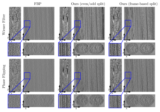
Figure 9: Output of our method when using the even/odd and frame-based splitting approach for the tilt series. All experimental details are as described in Section 2.2.2 and Appendix C.2.

References

- [BBS20] Tamir Bendory, Alberto Bartesaghi and Amit Singer “Single-Particle Cryo-Electron Microscopy: Mathematical Theory, Computational Challenges, and Opportunities” In IEEE Signal Processing Magazine 37.2, 2020, pp. 58–76
- [Bep+20] Tristan Bepler, Kotaro Kelley, Alex J Noble and Bonnie Berger “Topaz-Denoise: General Deep Denoising Models for CryoEM and CryoET” In Nature Communications 11.1, 2020, pp. 1–12
- [BS16] Tanmay A M Bharat and Sjors H W Scheres “Resolving Macromolecular Structures From Electron Cryo-Tomography Data Using Subtomogram Averaging in RELION” In Nature Protocols 11.11, 2016, pp. 2054–2065
- [BBC22] Jan Böhning, Tanmay AM Bharat and Sean M Collins “Compressed Sensing for Electron Cryotomography and High-Resolution Subtomogram Averaging of Biological Specimens” In Structure 30.3, 2022, pp. 408–417
- [Buc+19] Tim-Oliver Buchholz, Mareike Jordan, Gaia Pigino and Florian Jug “Cryo-Care: Content-Aware Image Restoration for Cryo-Transmission Electron Microscopy Data” In International Symposium on Biomedical Imaging, 2019
- [Den+16] Yuchen Deng, Yu Chen, Yan Zhang, Shengliu Wang, Fa Zhang and Fei Sun “ICON: 3D Reconstruction With ‘Missing-Information’ Restoration in Biological Electron Tomography” In Journal of Structural Biology 195.1, 2016, pp. 100–112
- [Din+19] Guanglei Ding, Yitong Liu, Rui Zhang and Huolin L Xin “A Joint Deep Learning Model to Recover Information and Reduce Artifacts in Missing-Wedge Sinograms for Electron Tomography and Beyond” In Scientific Reports 9.1, 2019, pp. 1–13
- [Fra21] Achilleas S Frangakis “It’s Noisy Out There! A Review of Denoising Techniques in Cryo-Electron Tomography” In Journal of Structural Biology 213.4, 2021, pp. 107804
- [Gub+20] Ilja Gubins, Marten L Chaillet, Gijs Schot, Remco C Veltkamp, Friedrich Förster, Yu Hao, Xiaohua Wan, Xuefeng Cui, Fa Zhang and Emmanuel Moebel “SHREC 2020: Classification in Cryo-Electron Tomograms” In Computers & Graphics 91 Elsevier, 2020, pp. 279–289
- [HH18] Reinhard Heckel and Paul Hand “Deep Decoder: Concise Image Representations from Untrained Non-Convolutional Networks” In International Conference on Learning Representations, 2018
- [HS20] Reinhard Heckel and Mahdi Soltanolkotabi “Compressive Sensing With Un-Trained Neural Networks: Gradient Descent Finds a Smooth Approximation” In International Conference on Machine Learning, 2020
- [HS20a] Reinhard Heckel and Mahdi Soltanolkotabi “Denoising and Regularization via Exploiting the Structural Bias of Convolutional Generators” In International Conference on Learning Representations, 2020
- [Hen+21] Allard A Hendriksen, Dirk Schut, Willem Jan Palenstijn, Nicola Viganó, Jisoo Kim, Daniël M Pelt, Tristan Van Leeuwen and K Joost Batenburg “Tomosipo: Fast, Flexible, and Convenient 3D Tomography for Complex Scanning Geometries in Python” In Optics Express 29.24, 2021, pp. 40494–40513
- [Hon+23] Ye Hong, Yutong Song, Zheyuan Zhang and Sai Li “Cryo-Electron Tomography: The Resolution Revolution and a Surge of in Situ Virological Discoveries” In Annual Review of Biophysics 52, 2023, pp. 339–360
- [KB15] Diederik P. Kingma and Jimmy Ba “Adam: A Method for Stochastic Optimization.” In International Conference on Learning Representations, 2015
- [KAH23] Tobit Klug, Dogukan Atik and Reinhard Heckel “Analyzing the Sample Complexity of Self-Supervised Image Reconstruction Methods” In Conference on Neural Information Processing Systems, 2023, to appear
- [KMM96] James R. Kremer, David N. Mastronarde and J.Richard McIntosh “Computer Visualization of Three-Dimensional Image Data Using IMOD” In Journal of Structural Biology 116.1, 1996, pp. 71–76
- [Leh+18] Jaakko Lehtinen, Jacob Munkberg, Jon Hasselgren, Samuli Laine, Tero Karras, Miika Aittala and Timo Aila “Noise2Noise: Learning Image Restoration Without Clean Data” In International Conference on Machine Learning, 2018
- [LHZ23] Yun-Tao Liu, Jason Hu and Z Hong Zhou “Resolving the Preferred Orientation Problem in CryoEM Reconstruction with Self-Supervised Deep Learning” In Microscopy and Microanalysis 29.Supplement_1, 2023, pp. 1918–1919
- [Liu+22] Yun-Tao Liu, Heng Zhang, Hui Wang, Chang-Lu Tao, Guo-Qiang Bi and Z Hong Zhou “Isotropic Reconstruction for Electron Tomography With Deep Learning” In Nature Communications 13.1, 2022, pp. 6482
- [Mal+23] Jeronimo Carvajal Maldonado, Lorenz Lamm, Ye Liu, Yu Liu, Ricardo D. Righetto, Julia A. Schnabel and Tingying Peng “F2FD: Fourier Perturbations for Denoising Cryo-Electron Tomograms and Comparison to Established Approaches” In 2023 IEEE 20th International Symposium on Biomedical Imaging, 2023
- [Mal93] Tom Malzbender “Fourier Volume Rendering” In ACM Transactions on Graphics (TOG) 12.3, 1993, pp. 233–250
- [MC23] Charles Millard and Mark Chiew “A Theoretical Framework for Self-Supervised MR Image Reconstruction Using Sub-Sampling via Variable Density Noisier2Noise” In IEEE Transactions on Computational Imaging 9, 2023, pp. 707–720
- [MC22] Charles Millard and Mark Chiew “Simultaneous Self-Supervised Reconstruction and Denoising of Sub-Sampled MRI Data With Noisier2Noise”, 2022 arXiv:2210.01696 [eess.IV]
- [Mor+20] Nick Moran, Dan Schmidt, Yu Zhong and Patrick Coady “Noisier2Noise: Learning to Denoise From Unpaired Noisy Data” In IEEE Conference on Computer Vision and Pattern Recognition, 2020
- [Rad88] Michael Radermacher “Three-Dimensional Reconstruction of Single Particles From Random and Nonrandom Tilt Series” In Journal of Electron Microscopy Technique 9.4, 1988, pp. 359–394
- [RFB15] Olaf Ronneberger, Philipp Fischer and Thomas Brox “U-Net: Convolutional Networks for Biomedical Image Segmentation” In The Medical Image Computing and Computer Assisted Intervention, 2015
- [Sig16] Fred J. Sigworth “Principles of Cryo-EM Single-Particle Image Processing” In Microscopy 65.1, 2016, pp. 57–67
- [TC19] Dimitry Tegunov and Patrick Cramer “Real-Time Cryo-Electron Microscopy Data Preprocessing With Warp” In Nature Methods 16.11, 2019, pp. 1146–1152
- [TB20] Martin Turk and Wolfgang Baumeister “The Promise and the Challenges of Cryo-Electron Tomography” In FEBS Letters 594.20, 2020, pp. 3243–3261
- [UVL18] Dmitry Ulyanov, Andrea Vedaldi and Victor Lempitsky “Deep Image Prior” In IEEE Conference on Computer Vision and Pattern Recognition, 2018
- [WB16] W Wan and John AG Briggs “Cryo-Electron Tomography and Subtomogram Averaging” In Methods in Enzymology 579, 2016, pp. 329–367
- [Yan+19] Rui Yan, Singanallur V Venkatakrishnan, Jun Liu, Charles A Bouman and Wen Jiang “MBIR: A Cryo-Et 3D Reconstruction Method That Effectively Minimizes Missing Wedge Artifacts and Restores Missing Information” In Journal of Structural Biology 206.2, 2019, pp. 183–192
- [Zan+09] Giulia Zanetti, James D. Riches, Stephen D. Fuller and John A.G. Briggs “Contrast Transfer Function Correction Applied to Cryo-Electron Tomography and Sub-Tomogram Averaging” In Journal of Structural Biology 168.2, 2009, pp. 305–312
- [Zha+23] Haonan Zhang, Yan Li, Yanan Liu, Dongyu Li, Lin Wang, Kai Song, Keyan Bao and Ping Zhu “A Method for Restoring Signals and Revealing Individual Macromolecule States in Cryo-Et, REST” In Nature Communications 14.1, 2023, pp. 2937