Embedding Space Interpolation Beyond Mini-Batch,
Beyond Pairs and Beyond Examples

Abstract

Mixup refers to interpolation-based data augmentation, originally motivated as a way to go beyond empirical risk minimization (ERM). Its extensions mostly focus on the definition of interpolation and the space (input or embedding) where it takes place, while the augmentation process itself is less studied. In most methods, the number of generated examples is limited to the mini-batch size and the number of examples being interpolated is limited to two (pairs), in the input space.

We make progress in this direction by introducing MultiMix, which generates an arbitrarily large number of interpolated examples beyond the mini-batch size, and interpolates the entire mini-batch in the embedding space. Effectively, we sample on the entire convex hull of the mini-batch rather than along linear segments between pairs of examples.

On sequence data we further extend to Dense MultiMix. We densely interpolate features and target labels at each spatial location and also apply the loss densely. To mitigate the lack of dense labels, we inherit labels from examples and weight interpolation factors by attention as a measure of confidence.

Overall, we increase the number of loss terms per mini-batch by orders of magnitude at little additional cost. This is only possible because of interpolating in the embedding space. We empirically show that our solutions yield significant improvement over state-of-the-art mixup methods on four different benchmarks, despite interpolation being only linear. By analyzing the embedding space, we show that the classes are more tightly clustered and uniformly spread over the embedding space, thereby explaining the improved behavior.

1 Introduction

Mixup [zhang2018mixup] is a data augmentation method that interpolates between pairs of training examples, thus regularizing a neural network to favor linear behavior in-between examples. Besides improving generalization, it has important properties such as reducing overconfident predictions and increasing the robustness to adversarial examples. Several follow-up works have studied interpolation in the latent or embedding space, which is equivalent to interpolating along a manifold in the input space [verma2019manifold], and a number of nonlinear and attention-based interpolation mechanisms [yun2019cutmix, kim2020puzzle, kim2021co, uddin2020saliencymix, chen2022transmix]. However, little progress has been made in the augmentation process itself, i.e., the number $n$ of generated examples and the number $m$ of examples being interpolated.

Mixup was originally motivated as a way to go beyond empirical risk minimization (ERM) [Vapn99] through a vicinal distribution expressed as an expectation over an interpolation factor $\lambda$, which is equivalent to the set of linear segments between all pairs of training inputs and targets. In practice however, in every training iteration, a single scalar $\lambda$ is drawn and the number of interpolated pairs is limited to the size $b$ of the mini-batch ($n=b$), as illustrated in Figure 1(a). This is because if interpolation takes place in the input space, it would be expensive to increase the number of pairs per iteration. To our knowledge, these limitations exist in all mixup methods.

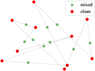
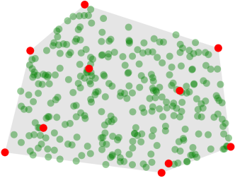
(a) mixup	(b) MultiMix (ours)

Figure 1: Data augmentation in a mini-batch $B$ of $b=10$ points in two dimensions. (a) mixup: sampling $n=b$ points on linear segments between $b$ pairs of points using the same interpolation factor $\lambda$. (b) MultiMix: sampling $n=300$ points in the convex hull of $B$.

In this work, we argue that a data augmentation process should increase the data seen by the model, or at least by its last few layers, as much as possible. In this sense, we follow manifold mixup [verma2019manifold] and generalize it in a number of ways to introduce MultiMix.

First, we increase the number $n$ of generated examples beyond the mini-batch size $b$, by orders of magnitude ($n\gg b$). This is possible by interpolating at the deepest layer, i.e., just before the classifier, which happens to be the most effective choice. To our knowledge, we are the first to investigate $n>b$.

Second, we increase the number $m$ of examples being interpolated from $m=2$ (pairs) to $m=b$ (a single tuple containing the entire mini-batch). Effectively, instead of linear segments between pairs of examples in the mini-batch, we sample on their entire convex hull as illustrated in Figure 1(b). This idea has been investigated in the input space: the original mixup method [zhang2018mixup] found it non-effective, while [Dabouei_2021_CVPR] found it effective only up to $m=3$ examples and [abhishek2022multi] went up to $m=25$ but with very sparse interpolation factors. To our knowledge, we are the first to investigate $m>2$ in the embedding space and to show that it is effective up to $m=b$.

Third, instead of using a single scalar value of $\lambda$ per mini-batch, we draw a different vector $\lambda\in{}^{m}$ for each interpolated example. A single $\lambda$ works for standard mixup because the main source of randomness is the choice of pairs (or small tuples) out of $b$ examples. In our case, because we use a single tuple of size $m=b$, the only source of randomness being $\lambda$.

Method	Space	Terms	Mixed	Fact	Distr
Mixup [zhang2018mixup]	input	$b$	$2$	$1$	Beta
Manifold mixup [verma2019manifold]	embedding	$b$	$2$	$1$	Beta
$\zeta$-Mixup [abhishek2022multi]	input	$b$	$25$	$1$	RandPerm
SuperMix [Dabouei_2021_CVPR]	input	$b$	$3$	$1$	Dirichlet
MultiMix (ours)	embedding	$n$	$b$	$n$	Dirichlet
Dense MultiMix (ours)	embedding	$nr$	$b$	$nr$	Dirichlet

Table 1: Interpolation method properties. Space: Space where interpolation takes place; Terms: number of loss terms per mini-batch; Mixed: maximum number $m$ of examples being interpolated; Fact: number of interpolation factors $\lambda$ per mini-batch; Distr: distribution used to sample interpolation factors; RandPerm: random permutations of a fixed discrete probability distribution. $b$: mini-batch size; $n$: number of generated examples per mini-batch; $r$: spatial resolution.

We also argue that, what matters more than the number of (interpolated) examples is the total number of loss terms per mini-batch. A common way to increase the number of loss terms per example is by dense operations when working on sequence data, e.g. patches in images or voxels in video. This is common in dense tasks like segmentation [noh2015learning] and less common in classification [kim2021keep]. We are the first to investigate this idea in mixup, introducing Dense MultiMix.

In particular, this is an extension of MultiMix where we work with feature tensors of spatial resolution $r$ and densely interpolate features and targets at each spatial location, generating $r$ interpolated features per example and $nr>n$ per mini-batch. We also apply the loss densely. This increases the number of loss terms further by a factor $r$, typically one or two orders of magnitude, compared with MultiMix. Of course, for this to work, we also need a target label per feature, which we inherit from the corresponding example. This is a weak form of supervision [ZZY+18]. To carefully select the most representative features per object, we use an attention map representing our confidence in the target label per spatial location. The interpolation vectors $\lambda$ are then weighted by attention.

Table 1 summarizes the properties of our solutions against existing interpolation methods. Overall, we make the following contributions:

1. We generate an arbitrary large number of interpolated examples beyond the mini-batch size, each by interpolating the entire mini-batch in the embedding space, with one interpolation vector per example. (subsection 3.2).

2. We extend to attention-weighted dense interpolation in the embedding space, further increasing the number of loss terms per example (LABEL:sec:dense).

3. We improve over state-of-the-art (SoTA) mixup methods on image classification, robustness to adversarial attacks, object detection and out-of-distribution detection. Our solutions have little or no additional cost while interpolation is only linear (LABEL:sec:exp).

4. Analysis of the embedding space shows that our solutions yield classes that are tightly clustered and uniformly spread over the embedding space (LABEL:sec:exp).

2 Related Work

Mixup: interpolation methods

In general, mixup interpolates between pairs of input examples [zhang2018mixup] or embeddings [verma2019manifold] and their corresponding target labels. Several follow-up methods mix input images according to spatial position, either at random rectangles [yun2019cutmix] or based on attention [uddin2020saliencymix, kim2020puzzle, kim2021co], in an attempt to focus on a different object in each image. Other follow-up method [liu2022tokenmix] randomly cuts image at patch level and obtains its corresponding mixed label using content-based attention. We also use attention in our dense MultiMix variant, but in the embedding space. Other definitions of interpolation include the combination of content and style from two images [hong2021stylemix], generating out-of-manifold samples using adaptive masks [liu2022automix], generating binary masks by thresholding random low-frequency images [harris2020fmix] and spatial alignment of dense features [venkataramanan2021alignmix]. Our dense MultiMix also uses dense features but without aligning them and can interpolate a large number of samples, thereby increasing the number of loss-terms per example. Our work is orthogonal to these methods as we focus on the sampling process of augmentation rather than on the definition of interpolation. We refer the reader to [li2022openmixup] for a comprehensive study of mixup methods.

Mixup: number of examples to interpolate

To the best of our knowledge, the only methods that interpolate more than two examples for image classification are OptTransMix [zhu2020automix], SuperMix [Dabouei_2021_CVPR], $\zeta$-Mixup [abhishek2022multi] and DAML [shu2021open]. All these methods operate in the input space and limit the number of generated examples to the mini-batch size; whereas MultiMix generates an arbitrary number of interpolated examples (more than $1000$ in practice) in the embedding space. To determine the interpolation weights, OptTransMix uses a complex optimization process and only applies to images with clean background; $\zeta$-Mixup uses random permutations of a fixed vector; SuperMix uses a Dirichlet distribution over not more than $3$ examples in practice; and DAML uses a Dirichlet distribution to interpolate across different domains. We also use a Dirichlet distribution but over as many examples as the mini-batch size. Similar to MultiMix, [carratino2022mixup] uses different $\lambda$ within a single batch. Beyond classification, $m$-Mix [zhang2022m] uses graph neural networks in a self-supervised setting with pair-based loss functions. The interpolation weights are deterministic and based on pairwise similarities.

Number of loss terms

Increasing the number of loss terms more than $b$ per mini-batch is not very common in classification. In deep metric learning [musgrave2020metric, kim2020proxy, wang2019multi], it is common to have a loss term for each pair of examples in a mini-batch in the embedding space, giving rise to $b(b-1)/2$ loss terms per mini-batch, even without mixup [venkataramanan2021takes]. Contrastive loss functions are also common in self-supervised learning [chen2020simple, caron2020unsupervised] but have been used for supervised image classification too [khosla2020supervised]. Ensemble methods [wen2020batchensemble, dusenberry2020efficient, havasi2020training, allingham2021sparse] increase the number of loss terms, but with the proportional increase of the cost by operating in the input space. To our knowledge, MultiMix is the first method to increase the number of loss terms per mini-batch to $n\gg b$ for mixup. Dense MultiMix further increases this number to $nr$. By operating in the embedding space, their computational overhead is minimal.

Dense loss functions

Although standard in dense tasks like semantic segmentation [noh2015learning, he2017mask], where dense targets commonly exist, dense loss functions are less common otherwise. Few examples are in weakly-supervised segmentation [ZZY+18, AhCK19], few-shot learning [Lifchitz_2019_CVPR, Li_2019_CVPR], where data augmentation is of utter importance, attribution methods [kim2021keep] and unsupervised representation learning, e.g. dense contrastive learning [o2020unsupervised, Wang_2021_CVPR], learning from spatial correspondences [xiong2021self, xie2021propagate] and masked language or image modeling [bert, xie2021simmim, li2021mst, zhou2021ibot]. To our knowledge, we are the first to use dense interpolation and a dense loss function for mixup.

3 Method

3.1 Preliminaries and background

Problem formulation

Let $x\in\mathcal{X}$ be an input example and $y\in\mathcal{Y}$ its one-hot encoded target, where $\mathcal{X}={}^{D}$ is the input space, $\mathcal{Y}=\{0,1\}^{c}$ and $c$ is the total number of classes. Let $f_{\theta}:\mathcal{X}\to{}^{d}$ be an encoder that maps the input $x$ to an embedding $z=f_{\theta}(x)$, where $d$ is the dimension of the embedding. A classifier $g_{W}:{}^{d}\to\Delta^{c-1}$ maps $z$ to a vector $p=g_{W}(z)$ of predicted probabilities over classes, where $\Delta^{n}\subset{}^{n+1}$ is the unit $n$-simplex, i.e., $p\geq 0$ and $\mathbf{1}_{c}^{\top}p=1$, and $\mathbf{1}_{c}\in{}^{c}$ is an all-ones vector. The overall network mapping is $f\mathrel{:=}g_{W}\circ f_{\theta}$. Parameters $(\theta,W)$ are learned by optimizing over mini-batches.

Given a mini-batch of $b$ examples, let $X=(x_{1},\dots,x_{b})\in{}^{D\times b}$ be the inputs, $Y=(y_{1},\dots,y_{b})\in{}^{c\times b}$ the targets and $P=(p_{1},\dots,p_{b})\in{}^{c\times b}$ the predicted probabilities of the mini-batch, where $P=f(X)\mathrel{:=}(f(x_{1}),\dots,f(x_{b}))$. The objective is to minimize the cross-entropy

$$H(Y,P)\mathrel{:=}-\mathbf{1}_{c}^{\top}(Y\odot\log(P))\mathbf{1}_{b}/b$$ (1)

of predicted probabilities $P$ relative to targets $Y$ averaged over the mini-batch, where $\odot$ is the Hadamard (element-wise) product. In summary, the mini-batch loss is

$$L(X,Y;\theta,W)\mathrel{:=}H(Y,g_{W}(f_{\theta}(X))).$$ (2)

The total number of loss terms per mini-batch is $b$.

Mixup

Mixup methods commonly interpolate pairs of inputs or embeddings and the corresponding targets at the mini-batch level while training. Given a mini-batch of $b$ examples with inputs $X$ and targets $Y$, let $Z=(z_{1},\dots,z_{b})\in{}^{d\times b}$ be the embeddings of the mini-batch, where $Z=f_{\theta}(X)$. Manifold mixup [verma2019manifold] interpolates the embeddings and targets by forming a convex combination of the pairs with interpolation factor $\lambda\in[0,1]$:

$$\widetilde{Z} =Z(\lambda I+(1-\lambda)\Pi)$$ (3)

$$\widetilde{Y} =Y(\lambda I+(1-\lambda)\Pi),$$ (4)

where $\lambda\sim\operatorname{Beta}(\alpha,\alpha)$, $I$ is the identity matrix and $\Pi\in{}^{b\times b}$ is a permutation matrix. Input mixup [zhang2018mixup] interpolates inputs rather than embeddings:

$$\widetilde{X}=X(\lambda I+(1-\lambda)\Pi).$$ (5)

Whatever the interpolation method and the space where it is performed, the interpolated data, e.g. $\widetilde{X}$ [zhang2018mixup] or $\widetilde{Z}$ [verma2019manifold], replaces the original mini-batch data and gives rise to predicted probabilities $\widetilde{P}=(p_{1},\dots,p_{b})\in{}^{c\times b}$ over classes, e.g. $\widetilde{P}=f(\widetilde{X})$ [zhang2018mixup] or $\widetilde{P}=g_{W}(\widetilde{Z})$ [verma2019manifold]. Then, the average cross-entropy $H(\widetilde{Y},\widetilde{P})$ (1) between the predicted probabilities $\widetilde{P}$ and interpolated targets $\widetilde{Y}$ is minimized. The number of generated examples per mini-batch is $n=b$, same as the original mini-batch size, and each is obtained by interpolating $m=2$ examples. The total number of loss terms per mini-batch is again $b$.

3.2 MultiMix

Interpolation

The number of generated examples per mini-batch is now $n\gg b$ and the number of examples being interpolated is $m=b$. Given a mini-batch of $b$ examples with embeddings $Z$ and targets $Y$, we draw interpolation vectors $\lambda_{k}\sim\operatorname{Dir}(\alpha)$ for $k=1,\dots,n$, where $\operatorname{Dir}(\alpha)$ is the symmetric Dirichlet distribution and $\lambda_{k}\in\Delta^{m-1}$, that is, $\lambda_{k}\geq 0$ and $\mathbf{1}_{m}^{\top}\lambda_{k}=1$. We then interpolate embeddings and targets by taking $n$ convex combinations over all $m$ examples:

$$\widetilde{Z} =Z\Lambda$$ (6)

$$\widetilde{Y} =Y\Lambda,$$ (7)

where $\Lambda=(\lambda_{1},\dots,\lambda_{n})\in{}^{b\times n}$. We thus generalize manifold mixup [verma2019manifold]:

1. from $b$ to an arbitrary number $n\gg b$ of generated examples: interpolated embeddings $\widetilde{Z}\in{}^{d\times n}$ (6) vs. ^d×b in (3), targets $\widetilde{Y}\in{}^{c\times n}$ (7) vs. ^c×b in (4);

2. from pairs ($m=2$) to a tuple of length $m=b$, containing the entire mini-batch: $m$-term convex combination (6),(7) vs. 2-term in (3),(4), Dirichlet vs. Beta distribution;

3. from fixed $\lambda$ across the mini-batch to a different $\lambda_{k}$ for each generated example.

Loss

Again, we replace the original mini-batch embeddings $Z$ by the interpolated embeddings $\widetilde{Z}$ and minimize the average cross-entropy $H(\widetilde{Y},\widetilde{P})$ (1) between the predicted probabilities $\widetilde{P}=g_{W}(\widetilde{Z})$ and the interpolated targets $\widetilde{Y}$ (7). Compared with (2), the mini-batch loss becomes

$$L_{M}(X,Y;\theta,W)\mathrel{:=}H(Y\Lambda,g_{W}(f_{\theta}(X)\Lambda)).$$ (8)

The total number of loss terms per mini-batch is now $n\gg b$.