A critical evaluation of the added value of increased horizontal resolution in the hectometric range on the simulation of the mountain boundary layer

Abstract

The horizontal grid spacing of numerical weather prediction models keeps decreasing towards the hectometric range. Although topography, land-use, and other static parameters are well-resolved, models have to be evaluated, because it cannot be assumed that higher horizontal resolution automatically yields better model performance. In this study, we perform limited-area simulations with the ICON model across horizontal grid spacings (1 km, 500 m, 250 m, 125 m) in the Inn Valley, Austria. Simulations are ran with two turbulence schemes - a 1D parameterization and a 3D Smagorinsky-type scheme. We evaluate the model across scales with observations of the valley boundary layer from the CROSSINN measurement campaign. This allows us to investigate whether increasing the horizontal resolution automatically improves the representation of the thermally-induced circulation, surface exchange, and other mountain boundary layer processes. The two turbulence schemes produce quite similar results across grid spacings, while differences are mostly found in the representation of the thermal structure of the valley atmosphere. The model keeps facing challenges for the correct simulation of scale interactions, and the 3D Smagorinsky scheme simulates a delayed evening transition of the up-valley flow. It is argued that the major difference between schemes actually emerges from the different surface transfer schemes, and the choice of boundary layer parameterization is secondary.

1 Introduction

The rise of computational power in the recent decades allows operational numerical weather prediction (NWP) and climate models to operate at the kilometric range [8, 52, 42, 64]. One of the benefits of smaller horizontal grid spacings is the possibility of a more realistic representation of topography in the model domains while avoiding the deep convection parameterization. The world is not flat [63] - mountainous terrain covers more than 60% of the Earth’s surface and therefore strongly affects, e.g., the surface-atmosphere exchange of heat, mass, moisture, and momentum. However, the mountain boundary layer is known to be very complex, where classical boundary-layer theory assumptions are violated [85, 53, 70] and multi-scale flow interactions prevail [38, 54, 4].

For numerical models, the correct representation of the underlying terrain is crucial. Simulations across grid spacings over idealized topography revealed that at least ten grid points across a valley on the model grid are necessary to resolve mountain boundary-layer processes accordingly [79]. This criterion is partly met by modern, state-of-the-art NWP models ($\Delta x$=1 km), because they are able to resolve the topography of major Alpine valleys (e.g., the Inn Valley in Austria or the Swiss Rhone Valley). This leads to a successful simulation of the thermally-induced circulation, especially the daytime up-valley flows [67, 21, 50]. However, real mountainous terrain consists of more than the major valleys (i.e., peak-to-peak distance of more than 10 km), with smaller tributary valleys and basins. Therefore, a decrease of $\Delta x$ towards the hectometric range ($\Delta x=\mathcal{O}{(100m)}$) is likely not only beneficial for the simulation of clouds and precipitation as suggested by [74], but also for an improved representation of atmospheric processes over truly complex terrain.

However, transitioning a model set-up towards the hectometric range introduces new challenges. [68] showed in a recent study in the Swiss Rhone Valley that a decrease of $\Delta x$ to 550 m results in a better simulation of the up-valley flows compared to the kilometric range - but only in combination with improved soil moisture initialization. This goes hand in hand that for high-resolution simulations, the correct representation of surface properties of soil and land-use with equally high-resolution datasets is crucial for successful simulation results [37, 26, 23].

Plenty real-case studies with simulations at the hectometric range over complex terrain exist, mostly for single events [12, 25, 29, to name a few]. However, only a few studies show a detailed model evaluation across several horizontal grid spacings over real terrain. [7] performed simulations at the hectometric range with the WRF model and found mostly an improved representation of vertical velocity and 2 m temperature; however, their study region was location over flat terrain. Nested set-ups over complex terrain exist, and suggest that higher-resolution runs lead to a better simulation of, e.g., horizontal wind speed or 2 m temperature [19, 44], but the focus of these studies was on different research questions. To our current knowledge, no study of a systematic model evaluation across grid spacings with a focus on flow structures exist over complex topography at the hectometric range.

In complex terrain, flow structures on several length and time scales are present and interact with each other. For example, larger-scale foehn flow removes a cold-air pool in a valley [27], the up-valley flow might erode smaller-scale slope flows [60], or a katabatic down-glacier wind is disturbed by gravity waves [23]. At the hectometric range, more small-scale flow structures can be expected to be resolved [14] - however, their interaction with larger-scale flows might not be represented correctly in the models [76, 23, 4]: For example, the cold-air pool is washed out too early, slope flows are eroded by a too strong up-valley flow, or the down-glacier wind is not simulated correctly in the first place. Simulated small-scale structures need to be resolved well to be “resilient" against larger-scale influence.

In order to correctly represent these multi-scale interactions, an appropriate representation of the surface heterogeneity and its coupling to the atmosphere above is required. This coupling in the models is handled through the surface-layer parameterization and the turbulence parameterization schemes. While surface-layer schemes that rely on the use of Monin-Obukhov similarity are questionable at such high resolution [75], our focus in the current work is on the turbulence scheme. A major issue emerging at the hectometric range is the so-called turbulence “grey zone" [83, 32, 11]: A part of the model’s turbulence is still parameterized, while another part is already resolved on the grid, leading to double-counting problems [34, 86]. The turbulence grey zone can be dealt with using scale-aware turbulence parameterizations [e.g., 16, 84, 36], however, we do not discuss them here because of their limited usage and instead focus on the classical 1D PBL and 3D Smagorinsky-type schemes.

How does one choose between a 1D TKE parameterization and a 3D LES closure? [33] suggest that the smallest physically acceptable scale for simulations of the convective boundary layer (CBL) over flat terrain is directly related to the boundary-layer height. [57] note that horizontal grid spacings smaller than the boundary-layer height range in the turbulence grey zone and that at $\Delta x<100$ m, a LES closure should be chosen. [79] argue that well-resolved model topography is more important than the choice of the boundary-layer parameterization. This is in agreement with [86], who stress that despite the challenges arising due to the turbulence grey zone, simulations over complex terrain at the hectometric range are worth pursuing due to the higher resolution of topography and land-use, leading to a better representation of surface exchange over complex terrain. However, the question which turbulence treatment should be chosen for the hectometric range over complex topography is still open.

Given the complex underlying terrain and the challenging representation of surface exchange in mountainous terrain, and that grey zone turbulence schemes might have their own limitations, we can try to answer the following questions:

• What are the challenges for the model in simulating the thermally-induced circulation?

• Is there an added value in increasing the model resolution?

• At which horizontal grid spacing should we switch to a full 3D turbulence scheme?

In this study, we employ a nested set-up of the Icosahedral Nonhydrostatic (ICON) Weather and Climate Model across several grid spacings over the hectometric range (1 km–125 m) over truly complex terrain, inspired by the idealized simulations of [79]. The area of interest is located in the Alps, namely the Inn Valley, Austria, where the CROSSINN measurement campaign took place in summer and autumn of 2019 [3]. Vertical profiles obtained from radiosondes, turbulence flux tower observations, and vertical profiles and co-planar scans of the wind structure observed by LIDARs allow us to evaluate how well the model is able to simulate the thermally-induced circulation in the valley. We test the model for two turbulence configurations (1D TKE scheme and a 3D LES Smagorinsky scheme). Generally speaking, we aim to deliver with this work a report on the current performance of a state-of-the-art NWP model at the hectometric range over complex topography.

The paper is organized as follows: In Section 2, we introduce the observational data from the measurement campaign and the numerical model set-up. In Section 3, we describe the model performance across scales by the means of cross-sections, vertical profiles, and timeseries of important meteorological variables, while we also discuss whether the findings from a single case study are generally representative. Section 4 includes the discussion, where we answer the aforementioned questions, while we draw the conclusions in Section 5.

2 Data and Methods

2.1 Observations

Our area of interest is located in the Inn Valley in the Austrian Alps, a large East-West oriented valley, with a peak-to-peak distance of around 10 km at our area of interest (Fig 1). The Inn Valley was subject to a rich body of mountain boundary layer research and will be a main target area for the upcoming TEAMx measurement campaign [61]. The Inn Valley is a primary location for strong up-valley flows [78, 39] and therefore an excellent location to investigate this mountain boundary layer phenomenon. The “i-Box" turbulence flux towers [62], located 30 km East of the city of Innsbruck, are operational since 2013 and allow a process-based model validation beyond standard model verification methods [21, 22].

In summer and autumn of 2019, the Cross-Valley Flow in the Inn Valley Investigated by Dual-Doppler Lidar Measurements (CROSSINN) campaign took place at the location of the i-Box stations [3], investigating besides the along-valley flows also mechanisms behind cross-valley circulations [6]. Besides the operational i-Box eddy covariance flux towers, the measurement campaign also provides observations from remote sensing systems such as LIDARs in vertical stare mode and coplanar scan modes; a HATPRO temperature profiler; and radiosonde launches and aircraft observations during intensive observation periods (IOPs). The location of the measurement sites is shown in Fig. 1: We will mostly utilize the collected data from the LIDAR observations, namely from the vertically pointing LIDARS SLXR 142 and SL 88 at the valley floor site (CS-VF0) and the coplanar scans across the valley [6, their Figure 1] retrieved from LIDARs located at CS-VF0, CS-SF11, and CS-NF27. Furthermore, use observations from three i-Box stations along the valley cross-section, namely from the valley floor (CS-VF0), the North-facing slope (CS-NF27), and the South-facing Slope (CS-SF11).

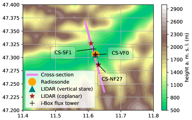
Figure 1: Overview of the measurement sites used in this study. The contour colors show the terrain, while the color dots represent the kind of observation (LIDAR, radiosonde, i-Box station). The purple line shows the valley cross-section used in the analysis of the model output in Figs. 4-7, 10, 12.

2.2 Numerical Model

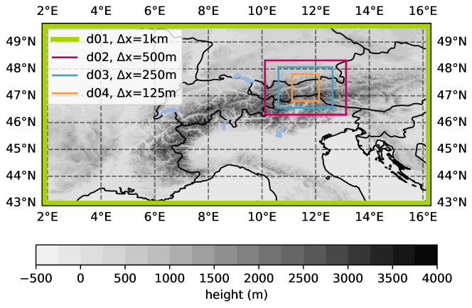
Figure 2: Grey contours: Model topography from the outermost domain at $\Delta x$=1 km. The boxes in color represent the location of the four model domains centered at the Inn Valley, Austria.

We employ a nested set-up of the ICOsahedral Non-hydrostatic (ICON) Weather and Climate Model version 2.6.5 [88]. As boundary conditions, we utilize ECMWF’s IFS forecast fields every hour, and we use MeteoSwiss’ COSMO-1 analysis fields ($\Delta x=1$ km) as initial conditions [67]. The model set-up contains four nested domains (Fig. 2, Tab. 1) with horizontal grid spacings of $\Delta x=1$ km (DX1000), $\Delta x=500$ m (DX500), $\Delta x=250$ m (DX250), and $\Delta x=125$ m (DX125). The outermost domain (DX1000) spans the Alps to ensure a correct representation of large-scale flow, while we subsequently nest down the domains by a factor two towards the domain of DX125, centered over Eastern part of the Inn Valley, Austria (Fig. 2). All domains use the same 80 vertical levels in terrain following SLEVE coordinates [41], with the lowest model level being located 20 m above ground. All simulations are started at 00:00 UTC of the respective case study day and are run for 24 hours in one-way nesting mode, while we regard the first three hours of simulation as model spin-up as in [23]. The dates for the case studies are 04 Aug 2019, 14 Aug 2019, 30 Aug 2019, 13 Sept 2019, and 14 Sept 2019.

Table 1: Overview of simulations conducted in this study.

Turbulence scheme	Simulations	horizontal grid spacing (m)
1D TKE [58]	1D-DX1000	1000
	1D-DX500	500
	1D-DX250	250
	1D-DX500	125
3D Smagorinsky [15]	3D-DX1000	1000
	3D-DX500	500
	3D-DX250	250
	3D-DX500	125

Since the model grid spacing is located at the hectometric range, high-resolution static input data is necessary to ensure realistic boundary layer development. For topography, we employ the ASTER dataset with a horizontal resolution of 30’ [55]. Compared to other widely used NWP models (e.g., WRF or COSMO), the ICON model is able run without numerical instabilities with slope angles steeper than 40^∘ because of its truly horizontal pressure gradient formulation [87]. This allows the model to stay numerically stable with steep slopes up to 70^∘ in idealized settings. In our simulations, no topographic filtering was necessary for the DX1000 and DX500 domains, while we had to apply filtering for DX250 and DX125 to ensure numerical stability. Still, maximum slope angles in all domains range over 45^∘, ensuring realistic representation of topograhy in the model.

For land use representation, most ICON model set-ups use the GLOBCOVER2009 dataset [29, 72]. We chose the CORINE land use dataset [17], because test simulations with CORINE yield improved model performance for the thermally-induced flows in the Inn Valley over GLOBCOVER. The soil is represented by the Harmonized World Soil database [18]. ICON is coupled to the multi-layer land surface scheme TERRA_ ML [69] and the lake model flake [51]. We utilize the ECRad scheme [30] as the radiation parameterization. Since our ICON set-up operates at horizontal grid spacings below 1 km, both the deep and shallow convection schemes are switched off to maintain physical consistency across resolutions.

We conduct two sensitivity runs for all case study days with two different turbulence parameterizations available in ICON (Tab. 1):

1. 1D TKE The standard turbulence scheme in ICON is “turbdiff" developed by [58] based on the work of [48, 49]. The scheme considers the vertical turbulent exchange with turbulence kinetic energy (TKE) as a prognostic variable and can be considered as a “classical" turbulence parameterization for NWP. The performance of the scheme is discussed in [10] and in [21, 22], where a detailed evaluation with TKE observations showed a satisfactory performance over complex topography at the kilometric range with the COSMO model. The turbulence scheme is coupled to a surface-transfer scheme also using prognostic TKE [9, Appendix B], which utilizes a tile approach for the computation of surface fluxes per grid cell [56, Chapter 3.8.11]. This allows a realistic representation of multiple land-use types per grid cell also for coarser grid spacings.

2. 3D Smagorinsky For large-eddy simulations, a Smagorinsky-type LES closure was implemented in ICON by [15] following [73] and [43]. This scheme assumes fully isotropic 3D turbulence, while the turbulence length scale depends on the Smagorinsky constant and the grid spacing $\Delta x$. A large-scale evaluation study of the 3D Smagorinsky scheme at $\Delta x=200$ m over Germany by [29] revealed that ICON is able to simulate realistic boundary layer development in real-case simulations. [72] evaluated ICON’s performance on precipitation cases and noticed satisfactory performance across resolutions, however noting that the highest resolution ($\Delta x$=100 m) simulated a too late onset of precipitation due to differences in cloud formation compared to coarser resolutions. Furthermore, the scheme is also utilized in high-resolution climate simulations at the kilometric range [74, 31] and is therefore not only applicable for the LES range ($\Delta x<$100 m). The turbulence scheme is coupled to a different surface transfer scheme than turbdiff following [46] without a tile approach for the computation of surface fluxes.

By applying both turbulence schemes in sensitivity runs for all case studies, we can assess their performance across scales. Furthermore, the detailed assessment allows us for recommendations on at which horizontal grid spacing the 3D Smagorinsky scheme starts adding value over the 1D TKE scheme.

3 Results

We are interested in days, when boundary-layer processes dominate and when a thermally-induced circulation is present in the Inn Valley. Thermally-induced flows were the subject of multiple idealized [e.g., 71, 65, 80, 59] and real-case numerical studies [e.g., 12, 81, 21, 22, 50] and can be considered as a well-known phenomenon in mountain meteorology; this makes thermally-induced flows an ideal test case for our analysis across grid spacings. A schematic overview of the thermally-induced circulation in the Inn Valley is shown in Fig. 3 for a better understanding of the phenomenon in the following Sections. During the night-time, down-valley and down-slope flows dominate the valley atmosphere. During daytime, the circulation reverses first with up-slope flows, and the up-valley flow starts at around 12 UTC. In general, cross-valley flow is also possible, mostly due to synoptic influences or the larger-scale Alpine pumping.

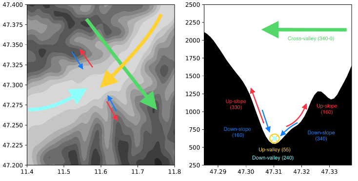
Figure 3: A schematic overview of the thermally-induced circulation in the Inn Valley. The left panel shows a top-down view, and the right panel shows a cross-section of the valley along the purple line in Fig. 1. The numbers in brackets show the estimated wind directions of the flow. Night-time flows are shown in blue (down-slope flows) and light blue (down-valley) colors. Daytime flows are shown in red (up-slope flows) and yellow (up-valley wind) colors. In the cross-section, the up-valley flow is shown as a yellow circle with an X, while the down-valley flow is shown as a light-blue point. Cross-valley flow is shown in green.

3.1 Case Study

We choose September 13, 2019 as a representative case study to give a detailed overview of ICON model performance. The general synoptic situation revealed a high-pressure ridge building up over central Europe, while a cut-off low was present over the Iberian Peninsula and a through present over the Balkans. The synoptic flow over the Alps was therefore weak and mostly Northerly-Northwesterly. September 13, 2019 was one of the CROSSINN IOPs, namely IOP8 [3], a cloud-free day with a well-developed up-valley flow in the afternoon (a webcam image of the area of interest at 12:00 local time can be seen at https://www.foto-webcam.eu/webcam/innsbruck-uni/2019/09/13/1200). Asides from the LIDAR and i-Box observations, radiosonde launches were performed every three hours starting from 03:00 UTC, allowing us a detailed evaluation of the vertical structure of the valley atmosphere.

3.1.1 How well does the model simulate the thermally-induced circulation?

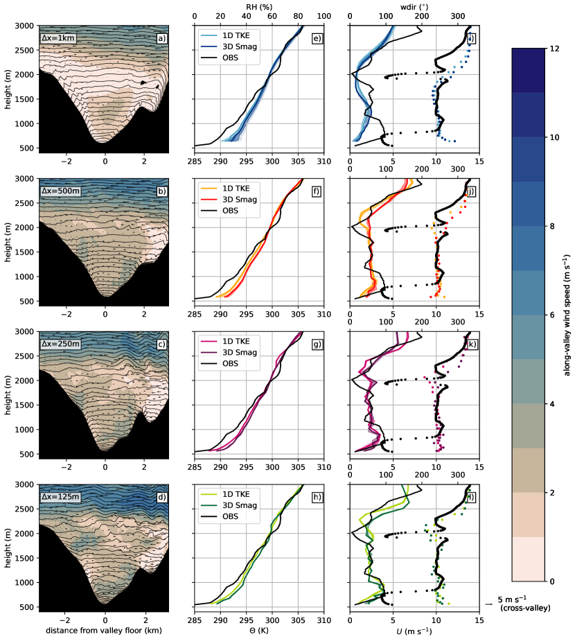
Figure 4: Vertical cross-section from model output of potential temperature (contours) and along-valley flow speed (colors) with 3D Smagorinsky following the purple line in Fig. 1 at 03:00 UTC across grid spacings (a-d). Panels e-f show radiosonde data (black lines) of potential temperature together with model output from from the closest model grid point for the two turbulence schemes (colored lines). The shaded areas around the colored lines show the 25 th/75 th (dark colours) and 10 th/90 th (light colours) percentiles of the grid-point ensemble. Panels g-j show the accompanying horizontal wind speeds (lines) and wind directions (points) together with radiosonde data.

At first, we investigate the representation of the thermally-induced circulation in the Inn Valley across the four grid spacings with the aid of radiosonde observations at four time representative of the state of the valley boundary layer (03:00 UTC, 09:00 UTC, 15:00 UTC, 20:00 UTC). Spatial heterogeneity in complex terrain raises the question whether one single (closest) grid point in the model domain is representative of the flow structure in a valley. Therefore, to gain an overview over spatial variability in the model, we employ the grid-point ensemble introduced by [21]: We calculate the 25 th, 75 th, 10 th and 90 th percentiles of the “next closest" grid points surrounding the closest grid point (determined via Euclidean distance).

In the night, at 03:00 UTC (Fig. 4), vertical cross-sections obtained via bi-variate spline interpolation of simulated potential temperature reveal that a stable boundary layer (SBL) is present in the valley, with a cold-air pool (CAP) at the valley floor. Wind speeds are generally low, with weak down-slope flows draining towards the valley floor. The representation of the CAP improves with smaller $\Delta x$, because the model’s warm bias reduces with increasing the horizontal resolution. The down-slope slope flows, visible in the downward-tilted isentropes close to the slopes (Fig. 4a-d), are also better resolved in the higher-resolution runs. The CAP and the nighttime SBL are also visible the observed vertical profile of potential temperature (Fig. 4e-h). The simulations agree with the observations, also simulating CAP at the valley floor, but the potential temperature values are overestimated for both turbulence schemes and across resolutions. The spread among the next closest grid points is quite large for DX1000, while it diminishes towards DX125. With decreasing $\Delta x$, the model simulates a stronger CAP, reducing the warm bias (Fig. 4h). This suggests that the model can simulate CAP formation more successfully at very high resolution (DX125) compared to the kilometric range (DX1000), even when the vertical grid spacing remains the same. This is in contrast with studies of dynamically-induced flows, where an increase in vertical grid levels yielded better model performance [77]. Observed and simulated horizontal wind speeds are generally low (Fig. 4i-l), while a low-level jet is visible in the lowest 550 m of the radiosonde observations. The model struggles to simulate this jet at the coarser grid spacings (e.g., DX1000 and DX500), while only the DX125 is able to represent the jet maximum both in magnitude and vertical extent (Fig. 4l). However, there are differences in the wind direction for all model runs: While the observations suggest an up-valley flow direction, the mode continuously simulates a down-valley flow (wind direction $\approx 270^{\circ}$). There are no large differences between the two turbulence schemes, although the 1D TKE scheme tends to simulate a “cooler" SBL by less than 1 K than the 3D Smagorinsky scheme. Still, both schemes across resolutions are not able to capture the observed minimum potential temperature at the valley floor.

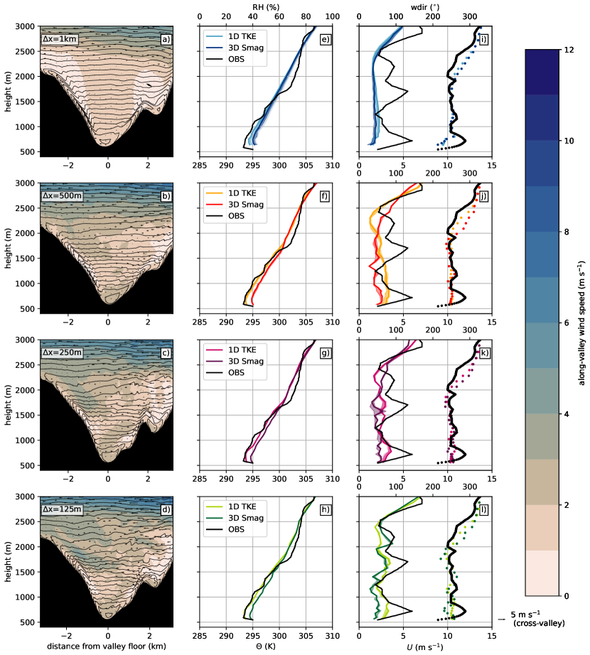
Figure 5: As Fig. 4, but for 09:00 UTC.

The situation changes under the influence of incoming solar radiation: the nighttime SBL dissolved and a CBL forms at the valley floor, visible in the unstable lowest layer at the valley floor with a vertical extent of around 500 m above ground (Fig. 5a-d). At both the North- and South-facing valley slopes, up-slope flows are visible in all simulations. The radiosonde observations reveal a multi-layer inversion structure in the valley, where at least three distinct inversion layers are visible (Fig. 5e-h). This structure is related to subsidence and re-circulation zones of the up-slope flows, also observed in the Rivera Valley [82]. In general, the 3D Smagorinsky runs reveal a warmer mixed layer (by about 1 K) than the 1D TKE runs. The simulation of the potential temperature profiles improves with decreasing grid spacing, but the potential temperature profile of DX125-3D is most realistic, with a clearly visible multiple-layer valley atmosphere (Fig. 5h). The observations show a distinct second inversion around 1700 m with warmer potential temperature aloft, which is not reproduced by the model. The observed and simulated wind speeds remain low, and the dominating wind direction at the lowest levels is still down-valley at upper levels (Fig. 5i-l). However, there is a slight disagreement below the mixed-layer height: the observations suggest a low-level wind speed maximum (with a turn in wind direction), which is missed by most of the simulations except the DX125-3D run (Fig. 5l).

At 15:00 UTC, the valley is mostly dominated by a strong up-valley flow (Fig. 6) with with a vertical extent of around 1000 m above ground and wind speed maxima above 10 m s^-1 (Fig. 6a-d). The up-slope flows are not visible anymore and the dominating wind direction below mountain crest height is Easterly, corresponding to up-valley flows. The thermal structure of the valley atmosphere reveals a stabilization and the vertical extent of the CBL is reduced compared to before noon according to the potential temperature profiles (Fig. 6e-h). This stabilization is also simulated by the model and as in the previous times (03:00 and 09:00 UTC), the representation of the potential temperature profile is best for the smallest grid spacings (DX125, Fig. 6h). The distinct inversion lowered to 1500 m, but is still not well represented in the model. Concerning the structure of the up-valley flow (Fig. 6i-l), the up-valley maximum is weakest at DX1000-1D with an underestimation of the magnitude and the vertical extent of the jet (Fig. 6i). It should be noted the there is less underestimation with the DX1000-3D, likely because 3D Smagorinsky is a full 3D LES closure and therefore also includes horizontal shear production, which is beneficial for the successful simulation of the up-valley flow [21, 22]. With decreasing $\Delta x$, the horizontal wind speed is not underestimated anymore; at DX500, the up-valley flow jet is almost perfectly simulated, while at DX250, it is even overestimated (Fig. 6j,k). The DX125 runs show still an overestimation of the jet maximum, but again a bit better than DX250. Overall, the up-valley flow jet can be seen as quite well-simulated, because the dominant length scales are already resolved at 1 km. The wind direction below crest height is Easterly, while above crest height (around 1000 m above ground), the wind direction turns to Northerly, in accordance with the larger-scale synoptic flow and the plain-to-mountain circulation.

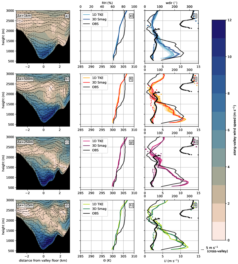
Figure 6: As Fig. 4, but for 15:00 UTC.

In the evening (20:00 UTC), the up-valley flow weakens and lifts, and the valley atmosphere stabilizes further (Fig 7). This stabilization is also present in the simulated potential temperature profiles (Fig 7e-h), but again with a warm bias, especially pronounced in DX250-3D and DX125-3D. The warmer valley atmosphere in the 3D Smagorinsky scheme likely prevents the growth of a shallow stable layer during the evening transition. However, the DX125-3D run manages to represent the adiabatic potential temperature layer below 1000 m, which is not captured by DX125-1D. As at 15:00 UTC, the vertical extent of the up-valley flow jet is underestimated at DX1000 together with a disagreement in the wind direction (Fig 7i). At the higher-resolution runs, the jet maximum is overestimated together with a misplaced peak, while the wind direction - still Easterly - is simulated correctly. In accordance with the warm bias, the 3D Smagorinsky scheme also simulates higher wind speeds at the ground and therefore a delayed evening transition. We will discuss this challenge in the next Sections in more detail.

To summarize, the model is able to simulate the general vertical structure of the thermally-induced circulation in the Inn Valley in a satisfying way. The benefit of higher-resolution runs lies in a better representation of the thermal structure of the valley - especially for CAPs and the typical multi-layer inversion structure of the valley boundary layer. The up-valley flow is underestimated in the DX1000 runs, but this issue disappears with decreasing $\Delta x$ - possibly due to the better represented topography and 3D mixing. On the one hand, the 3D Smagorinsky scheme simulates “warmer" potential temperature profiles and a delayed evening transition, but on the other hand, the scheme is clearly able to simulate the multi-layer valley atmosphere and the up-valley flow strength better than 1D TKE.

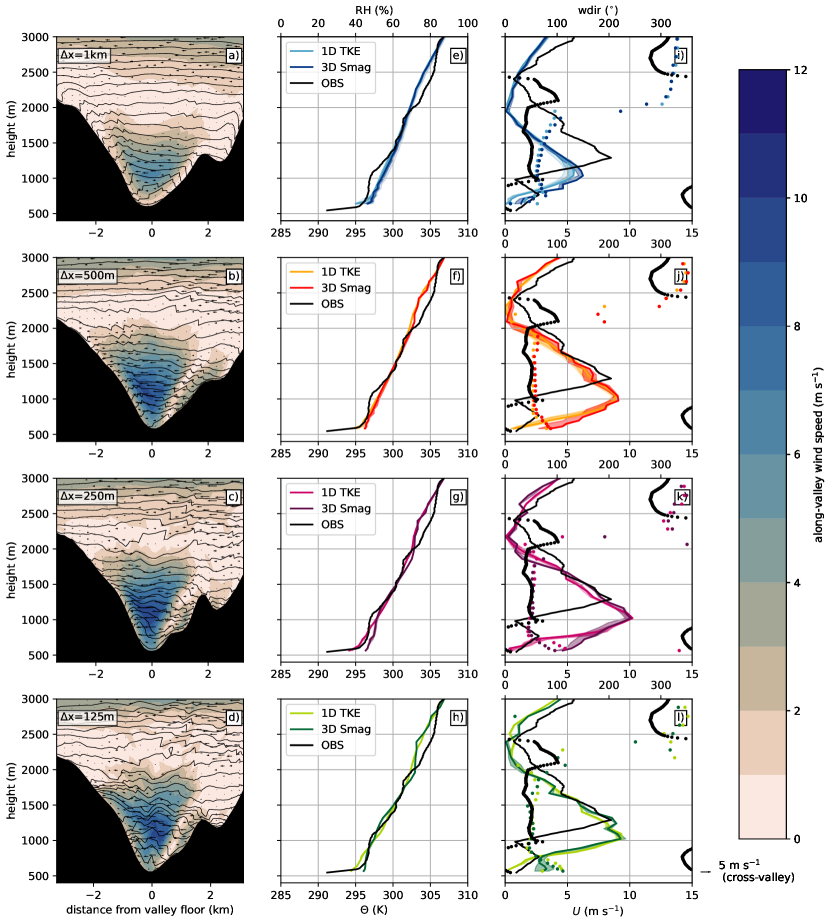
Figure 7: As Fig. 4, but for 20:00 UTC.

The vertical cross-sections with the radiosondes only reveal snapshots of the valley atmosphere, therefore we analyze timeseries of simulated horizontal wind speeds together with vertical LIDAR profiles (Fig. 8). Time series of observed wind speed and direction reveal that the valley floor is mainly dominated by down-valley flows during the night-time (Fig. 8a,b), successfully simulated by the model across resolutions and turbulence schemes. After sunrise, an observed (secondary) wind speed maximum is present at around 08:00 UTC, while the wind direction remains down-valley. While DX1000 fails to simulate this phenomenon, the higher-resolution runs are able to capture the higher wind speeds before noon, although the timing of the maximum is shifted. Unfortunately, no LIDAR observations are available from 05:00 UTC to 07:00 UTC to explore this secondary maximum, however, judging from the model output, it is likely that the model still underestimates the strength of the down-valley flow in this time period, as it was also visible in the vertical profiles (Fig 5i-l). The onset of the up-valley flow occurs at 12:00 UTC according to the observations, visible in the shift of wind direction from Westerlies (down-valley) towards Easterlies (up-valley). This up-valley flow onset is delayed by an hour in the simulations with the 1D TKE scheme; while the onset is almost on time in the 3D Smagorinsky scheme. Judging from the time series reveals an overestimation of 10 m wind speeds for all hectometric grid spacings for both turbulence schemes (DX500–DX125). An exception is DX1000-1D: The 10 m wind speed seems to be exceptionally well-simulated. However, when we compare the vertical structure of DX1000-1D (Fig 8c) with the LIDAR observations (Fig 8b), it is noticeable that the strength and vertical extent of the up-valley flow are underestimated by around 2 m s^-1.

The vertical structure of the up-valley flow is better represented by the hectometric resolutions (Fig 8d-f,j-l), while they are however, overestimated. This pattern changes during the evening transition after 18:00 UTC: The LIDAR observations show that the up-valley flow weakens and lifts (Fig 8b), while the wind direction corresponds to up-valley flows except for the lowest levels, where there is already a shift towards down-valley flows. In the model, there is a disagreement between observed and simulated wind directions in the evening for both schemes (Fig 8a,f): The 1D TKE scheme performs better in drop of horizontal wind speeds and the 3D Smagorinsky scheme simulates too high wind speeds after 18:00 UTC. The only exception is the DX1000-3D run, where the wind speed drops as in the observations (Fig 8i). However, in the DX125-3D run, the shift in wind direction is simulated successfully close to the surface (Fig 8l), while the two intermediate runs (DX500-3D and DX250-3D) keep showing up-valley flow directions after 18:00 UTC (Fig 8j,k). Therefore, we identify the evening transition in this particular case study as a challenge for the model - we will discuss further driving factors in Section 3.1.3.

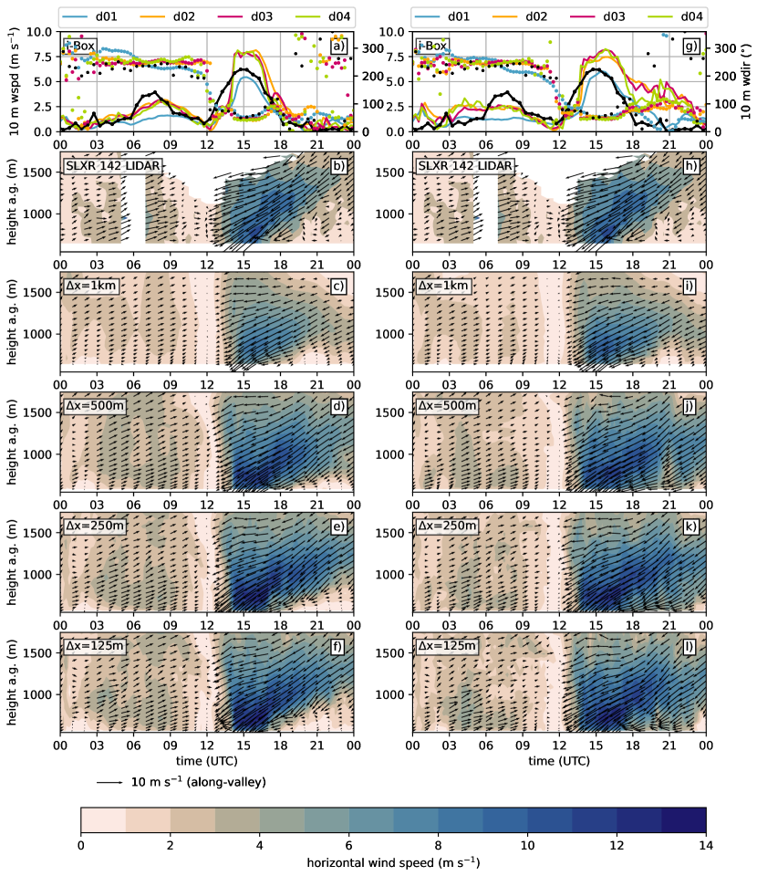
Figure 8: Panels a and b: Time series of wind speed and direction from observations from the i-Box flux tower located at the valley floor CS-VF0 (black lines/dots) with model output from the closest grid point (colors) for all domains from the 1D TKE scheme (panel a) and the 3D Smagorinsky scheme (panel g). Panels b and h: Observations of horizontal wind speed (colors) and wind direction (arrows) from the SLXR 142 Lidar located at the valley floor site. Corresponding time series from model output (colors) from the 1D TKE scheme (panels c-f) and the 3D Smagorinsky scheme (panels i-l).

3.1.2 Can the model simulate spatial variability?

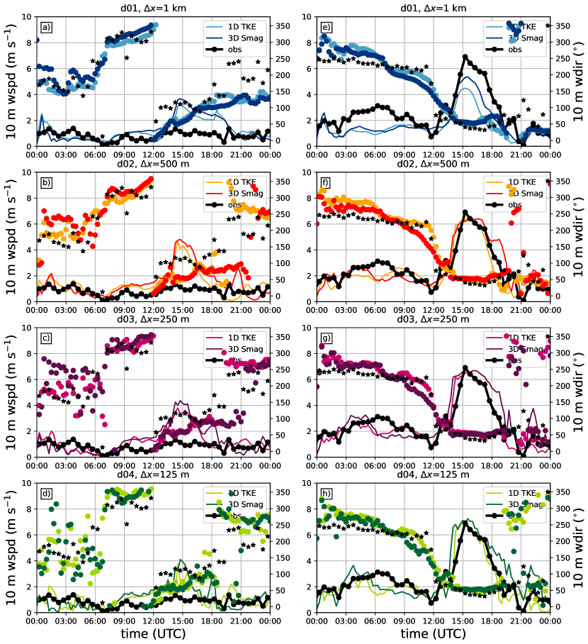
Figure 9: Timeseries of 10 m wind speed (lines) and direction (points) observations from the eddy covariance stations (black) and model output from the closest model grid point (colors) from the North-facing slope CS-NF27 (panels a-d) and the South-facing slope CS-SF1 (panels e-h).

In the previous Section we showed the model performance at the valley floor. However, in highly complex terrain, it is likely that one single point measurement is not representative for the boundary-layer structure in the entire valley. Therefore, we introduce time series of observations and model output across resolutions from the North-facing slope (CS-NF27, Fig 9a-d) and the South-facing slope (CS-SF11, Fig 9e-h).

The South-facing slope station (Fig 9e-h) shows a similar wind structure as at the valley floor. Down-valley flows dominate during the night-time and before noon, but the secondary maximum observed at the valley floor is not present. The up-valley flow arrives at 12:00 UTC with a sharp increase in wind speed and a shift in wind direction towards Easterlies. The model is underestimating the up-valley flow at DX1000-1D, while DX1000-3D is more successful in the simulation of the wind speed maximum (Fig 9e). In general, the wind speed maximum is well-simulated at the hectometric range, while the 3D Smagorinsky scheme manages to simulate a sharper wind speed increase with the arrival of the up-valley flow (Fig 9f-h). As at the valley floor station, the evening transition with the drop of the wind speed after 18:00 UTC is delayed in the runs 3D Smagorinsky scheme, although the delay is less pronounced than at the valley floor.

The wind speed observations at the North-facing slope station reveal a completely different structure than at the valley floor station (Fig. 8a,b): Horizontal wind speeds remain low (smaller than 2 m s^-1) during the entire night and day. The wind direction switches from down-slope before 06:00 UTC to up-slope flows until 12:00 UTC. After midday, the wind directions shifts towards up-valley while the wind speeds remain low, indicating that the up-slope flows are eroded by the larger-scale up-valley flow. The erosion of slope flows was also observed in the Rivera Valley [60] and is a common phenomenon at this particular slope station [21]. The correct simulation of the erosion of the slope flows depends on $\Delta x$: At DX1000, the up-valley flow is simulated too weakly as it is evident from the analysis of the (vertical) structure in the previous Section. However, the model simulates a wind maximum in the afternoon, synchronous with the up-valley flow maximum at the valley floor (Fig 9a). This structure is even more strongly simulated in the two intermediate domains (DX500 and DX250, Fig 9b,c). These results suggest that the model simulates a too strong slope flow erosion by the up-valley flow - and therefore facing a challenge with the scale interaction between the small-scale slope flows and the larger-scale up-valley flow. This shows that scale interactions are simulated in a more realistic way at higher resolutions due to the better representation of smaller scales.

To understand the reason for the simulated afternoon wind speed maximum at the North-facing slope better, we show cross-sections of the valley together with wind observations from LIDAR co-planar scans (Fig. 10). Observations from the cross-valley flow speed at 15:00 UTC (valley flow maximum) reveal a wind speed maximum (4 m s^-1) at the valley floor with North to South cross-valley flow (Fig. 10a,f). Between the heights of 500 m and 1500 m above ground, a cross-valley vortex with a re-circulation pattern is visible. The cross-valley vortex of the Inn Valley is the result of both thermal and dynamical forcing and forms due to a balance by the pressure gradient force and the centrifugal force due to the valley’s curvature [6]. The model is not able to reproduce this detailed cross-valley flow pattern at DX1000 (Fig. 10b,g): Although the modelled and observed cross-valley flow speeds and directions match, the model simulated a larger vertical extent of the wind speed maximum up to 1000 m above ground, while the observations reveal the re-circulation zone at this height. Furthermore, the horizontal extent of the cross-valley flow is larger - which, finally, leads to the too strong up-valley flow influence on the North-facing slope station. The simulations at the hectometric range (DX500 and DX250, (Fig. 10c-d,h-j) also show an overestimation of the cross-valley flow and its vertical and horizontal extent. Although there is a more detailed structure visible, the horizontal extent of the cross-valley flow is too strong leading to the erosion of the slope flows. At the highest resolution (DX125, Fig. 10e,j), the cross-valley flow is weaker again, leading to the best simulation of wind speeds at the North-facing slope station (Fig. 9d), but still overestimated.

To summarize, the model is able to simulate the general spatial variability of the flow structure in the valley cross-section. However, the model tends to simulate a too strong up-valley flow and the related cross-valley circulation at the hectometric range. This leads to the erosion of small-scale slope flows in the afternoon - and allows the conclusion that the model still struggles to simulate scale interactions between slope flows and up-valley flows correctly, even when the horizontal resolution is higher.

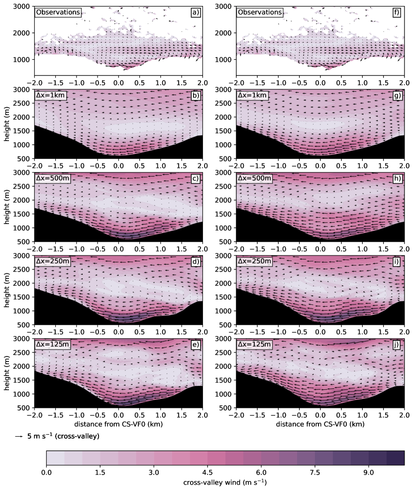
Figure 10: Panels a and f: Coplanar scans at 15:00 UTC from the Lidars located at the North-facing slope (CS-NF27), the valley floor (CS-VF0), and the South-facing slope (Mairbach), with observed cross-valley flow speeds (colors and wind arrows). Corresponding model output across resolutions and the two turbulence schemes (Panels b-e: 1D TKE; panels f-j: 3D Smagorinsky).

3.1.3 A Challenge: The Evening Transition

The case study evaluation showed that the model struggles to simulate the evening transition correctly, i.e., after the up-valley flow maximum at 15:00 UTC. Figure 8a shows that the observed horizontal wind speed at the valley floor decreases after 15:00 UTC. The wind speed decrease is delayed in the model, especially for the simulations with the 3D Smagorinsky scheme with a delay of up to 1 hour, and the wind speeds do not decrease down to less than 1 m s^-1 as in the observations and the simulations with the 1D TKE scheme. Therefore, the weakening of the up-valley flow and the transition back to down-valley flows poses a challenge for the model, and in the next few paragraphs, we explore the reasons for this delay.

The sensible heat (SH) flux is an important driver for boundary-layer development, and it can be spatially heterogeneous in flat [47] as well as in complex terrain [40]. Time series from SH flux observations accompanied by model output across grid spacings (Fig. 11a,g) reveal that SH fluxes are close to zero during the night-time (00:00-06:00 UTC). After sunrise, the SH fluxes become positive and they already reach their daytime maximum before noon, when the CBL is well-developed (Fig 5). In the afternoon, an untypical SH flux pattern emerges: The SH flux decreases after 11:00 UTC and turns negative at 15:00 UTC, synchronous with the up-valley flow maximum (Fig. 8). This behaviour on this sunny day is can be associated with the strong up-valley flow and advection processes and was also reported in previous valley wind studies [78, 60, 40, 6]. In the model, the major evolution of the SH flux is well-simulated; the magnitude, the timing, and the reversal to negative values in the afternoon are represented successfully in both turbulence schemes. The timing of the reversal of SH in the afternoon is better represented in the 3D Smagorisnky scheme, and there is a visible improvement in simulation with increasing resolution - while no such effect is visible in the 1D TKE scheme. The largest discrepancy between observed and simulated SH fluxes in the 3D scheme is visible after around 16:00 UTC (mostly for 3d-DX500 and 3D-DX250)- the time, when the actual evening transition takes place. Still, we conclude that the SH fluxes in the evening are not the major reason for the delayed eveing transition.

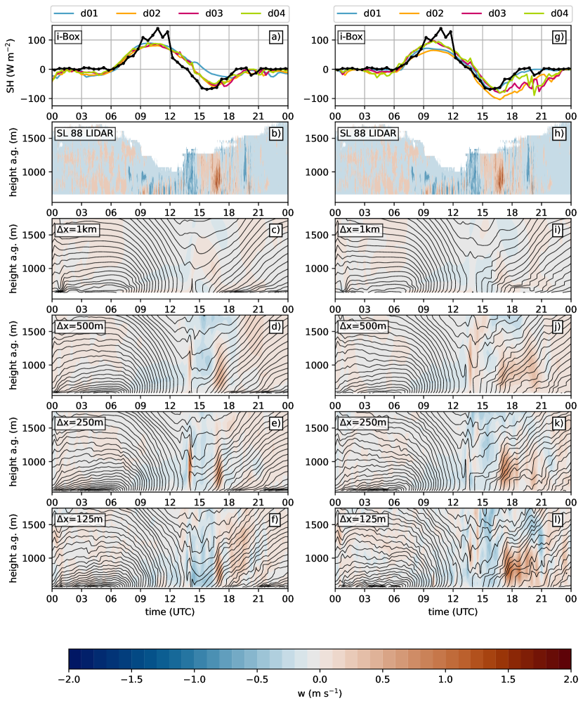
Figure 11: Panels a and f: Time series of sensible heat flux from observations from the i-Box flux tower at the valley floor CS-VF0 (black lines) with model output from the closest grid point (colors) from the 1D TKE scheme (panel a) and the 3D Smagorinsky scheme (panel f). Panels b and h: Observations of vertical wind speeds (colors) from the SL 88 Lidar located at the valley floor. Panels c-f, i-l: Corresponding vertical velocity (colors) and potential temperature (black contours) time series from model output from the 1D TKE scheme (c-f) and the 3D Smagorinsky scheme (i-l).

We now evaluate the vertical velocity behaviour at the valley floor and whether it corresponds to the SH structure. The SL 88 LIDAR at the valley floor performed scans in high temporal resolution of the wind components in vertical stare mode, including vertical velocities (Fig. 11b,h). According to the observations, vertical velocities are small in the night-time in in the first morning hours until around 08:00 UTC. After 08:00 UTC, the CBL at the valley floor develops with several smaller up- and downdrafts until around 13:00 UTC. When the up-valley flow arrives, the vertical velocities are mostly negative associated with subsidence at the valley floor, while after 15:00 UTC, mostly positive vertical velocities dominate. There is a distinct vertical velocity maximum visible at around 16:00 UTC, interestingly, when the SH flux reaches its minimum and the evening transition of the up-valley flow starts. During the evening transition, vertical velocities are mostly dominated by up- and downdrafts with a larger vertical extent than during the CBL phase before noon. After 21:00 UTC, vertical velocities become very small again.

The DX1000 runs only simulate a very crude vertical velocity structure for both turbulence schemes (Fig. 11c,i). This is not surprising, since it can not be expected that small-scale up- and downdrafts are resolved at $\Delta x$=1 km. DX500-1D and DX250-1D show a more detailed vertical velocity structure (Fig. 11d-e); suggesting subsidence during the CBL phase and an updraft when the up-valley flow arrives. This strong, unrealistic updraft might contribute to the overall too large horizontal and vertical extent of the simulated up-valley flow at these grid spacings (Fig. 8). At the start of the evening transition, DX500-1D and DX250-1D simulate the strong updraft at around 16:00 UTC correctly. The DX500-3D and DX250-3D runs (Fig. 11j-k) show a similar picture as their 1D counterparts, however, after the initial evening transition updraft, we note continuous positive vertical velocity values after 17:00 UTC, while in the observations, there are subsequent up- and downdrafts present. The evening transition in the 3D Smagorinsky runs is delayed, and the isentropes show that the growth of a SBL is prevented. However, the observations suggest one downdraft at around 20:00 UTC, which is also visible in the DX125-3D run, but one hour too late (21:00 UTC).

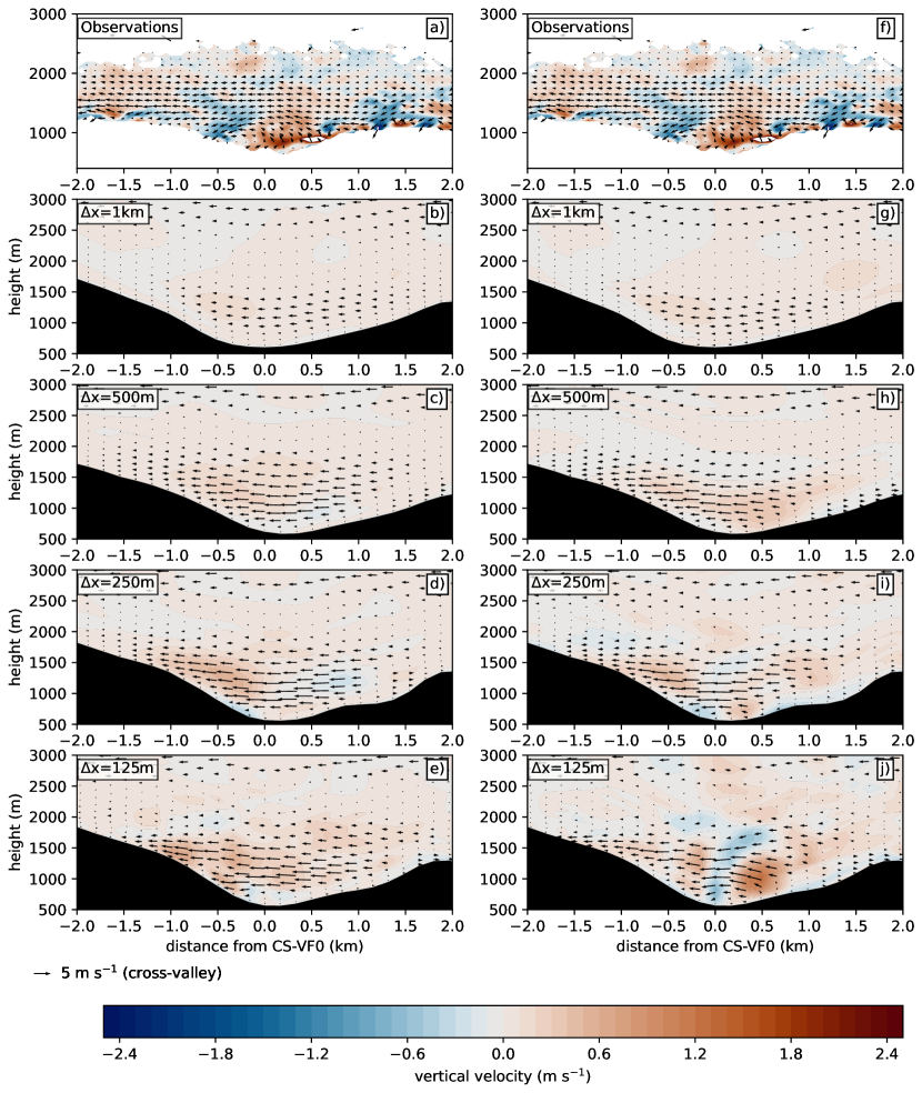
Figure 12: Panels a and f: Coplanar scans at 20:00 UTC from the Lidars located at the North-facing slope (CS-NF27), the valley floor (CS-VF0), and the South-facing slope (Mairbach) of vertical wind speed (color) and cross-valley flow speed (wind arrows). Corresponding model output across resolutions and the two turbulence schemes (1D TKE: panels b-e; 3D Smagorinsky: panels g-j).

To explore the atmospheric structure across the valley during the evening transition, we show coplanar scans of vertical velocity at 20:00 UTC (Fig. 12). The observed evening transition boundary layer shows a disorganized structure (Fig. 12a,f): While there is a distinct North-to-South cross-valley flow present, the vertical velocity pattern is dominated by up- and downdrafts at the slopes. At the valley floor, the observations show a major updraft above the valley floor, followed by a downdraft close to the North-facing slope. It is worth noting that all shown simulations (Fig. 12b-e,f-j), independent from the turbulence scheme, simulate a too strong cross-valley circulation without the observed re-circulation zone, while the coarser runs are unable to simulate the up- and downdrafts. However, DX125-3D (Fig. 12j) is the only simulation which manages to simulate a similar vertical velocity structure as in the observations, while the simulated up- and downdrafts seem to be spatially shifted compared to the observations. This explains the discrepancy in the time series of Fig 11; the fast-changing up-and downdrafts during the simulation are spatially and temporarily variable and therefore difficult to “pin down" to a certain point in space and time. Furthermore, the cross-valley flow speed is overestimated in the simulations beyond 1 km, especially for the DX125-3D run. We therefore think that the strong cross-valley flow component contributes to the delayed evening transition in the simulations. The main reason, however, is the representation of the surface in the 3D scheme as explained next.

A careful investigation of Figure 5 reveals that the boundary layer temperature in the 3D Smagorinksy scheme is relatively higher when a growing CBL is present in the valley. This is related to higher SH fluxes before noon than in the 1D TKE scheme (Fig. 11g). The higher SH flux results from larger heat transfer coefficients between the surface and the atmosphere (Fig. 13), which we believe is due to the difference in the way surface exchange is handled in the scheme. The result of the higher SH flux is a warmer valley atmosphere, which leads to a stronger pressure gradient between the valley and the surrounding alpine foreland (not shown). This allows a build-up of a stronger valley-wind circulation, especially visible in the vertical profiles of horizontal wind speed during the afternoon and evening (Figs. 6 and 7). Therefore, the most likely reason for the delayed evening transition in the 3D Smagorinsky scheme actually happens several hours before the evening: A warmer valley boundary layer leading to a stronger pressure gradient resulting in a stronger and more adler up-valley wind, which prevails longer than in the simulations with the 1D TKE scheme (delayed evening transition, Fig. 8g-l).

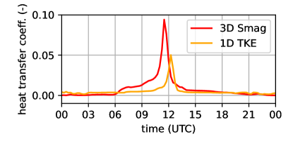
Figure 13: Time series of the dimensionless surface exchange coefficient for heat at the valley floor (CS-VF0). Only DX500 is shown but the behavior is similar for all other resolutions.

To summarize, the evening transition after the up-valley flow phase is a challenge for the model, since multiple scales interact with each other. The SH fluxes are simulated in a realistic way for both turbulence schemes and across resolutions. The simulation of vertical wind speeds improves with decreasing the horizontal grid spacing - finally, DX125-3D manages to simulate realistic vertical velocity structures in the cross-section, while the exact location of the up- and downdrafts is shifted. However, the reason for the delayed evening transition is a too stronger pressure gradient between the valley and the surrounding foreland leading to the formation of a too strong up-valley flow.

3.2 Average over 5 Days

3.2.1 Valley floor

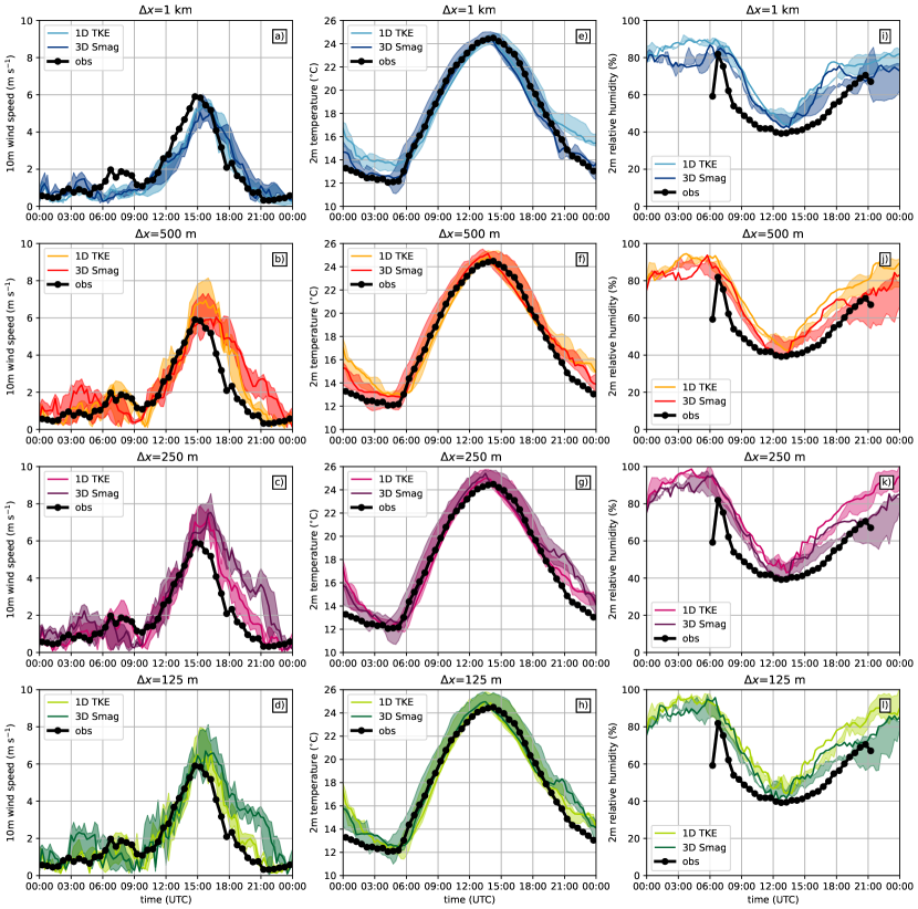
Figure 14: Average over five case study days at the valley floor station (CS-VF0) of 10 m wind speed (a-d), 2 m temperature (e-h), and 2 m relative humidity (i-l). Observations are shown in black dots, while colors indicate simulation output across $\Delta x$ and turbulence schemes. The straight lines indicate the median over the five days, and shaded areas indicate the 25 th and 75 th percentiles, respectively.

In the previous Section, we discussed the performance of the ICON model across horizontal grid spacings for only one case study of an IOP from the CROSSINN campaign. However, one single day is not representative for other up-valley flow days. Therefore, we perform a statistical analysis over the 5 case study days for common verification variables in model validation - namely, 10 m wind speed, 2 m temperature, and 2 m relative humidity.

Timeseries of the averaged meteorological variables at the valley floor station reveal a generally good performance for all grid spacings and turbulence closures (Fig. 14). A closer look at the 10 m wind speed (Fig. 14a-d) reveals similar features which were already observed for the single case study: Both DX1000-1D and DX-1000-3D simulate a delayed up-valley flow onset and an underestimated up-valley flow speed maximum. This problem disappears with the hectometric grid spacings, where DX500-1D and DX250-1D simulate the correct timing of the up-valley flow onset, but overestimate the maximum of the up-valley flow speed. Interestingly, 3D Smagorinsky performs better here; especially DX500-3D does simulate a realistic wind speed maximum. The smallest grid spacings perform similar as their coarser-resolution counterparts at the hectometric ranges. The delayed evening transition after the up-valley flow maximum is a challenge for the simulations with the 3D Smagorinsky scheme, and because the too strong pressure gradient (between valley and plain) is present simulations of all five case studies.

The diurnal cycle of 2 m temperature is represented well in the model across resolutions (Fig. 14e-h). The largest difference between observations and model output emerges in the night-time, when ICON simulates higher 2 m temperatures. This is a common problem in NWP [e.g., 28, 5], and also visible in the too weak stratification in the vertical potential temperature profiles (Fig. 5). The evening transition after 15:00 UTC is, interestingly, a challenge for the DX1000-1D run, while all the higher-resolution runs with the 1D scheme simulate the evening 2 m temperature well. In accordance with the too high wind speeds, the 2 m temperature in the evening (after 18:00 UTC) is overestimated in the runs with the 3D Smagorinsky scheme, in accordance with the higher wind speeds during the delayed evening transition.

The model performance for the diurnal cycle of 2 m relative humidity is similar across scales (Fig. 14i-l). However, simulations with the 3D Smagorinsky scheme perform better during daytime. Unfortunately, no observations of relative humidity are available from the flux tower during the night-time and the evening transition.

3.2.2 North-facing slope

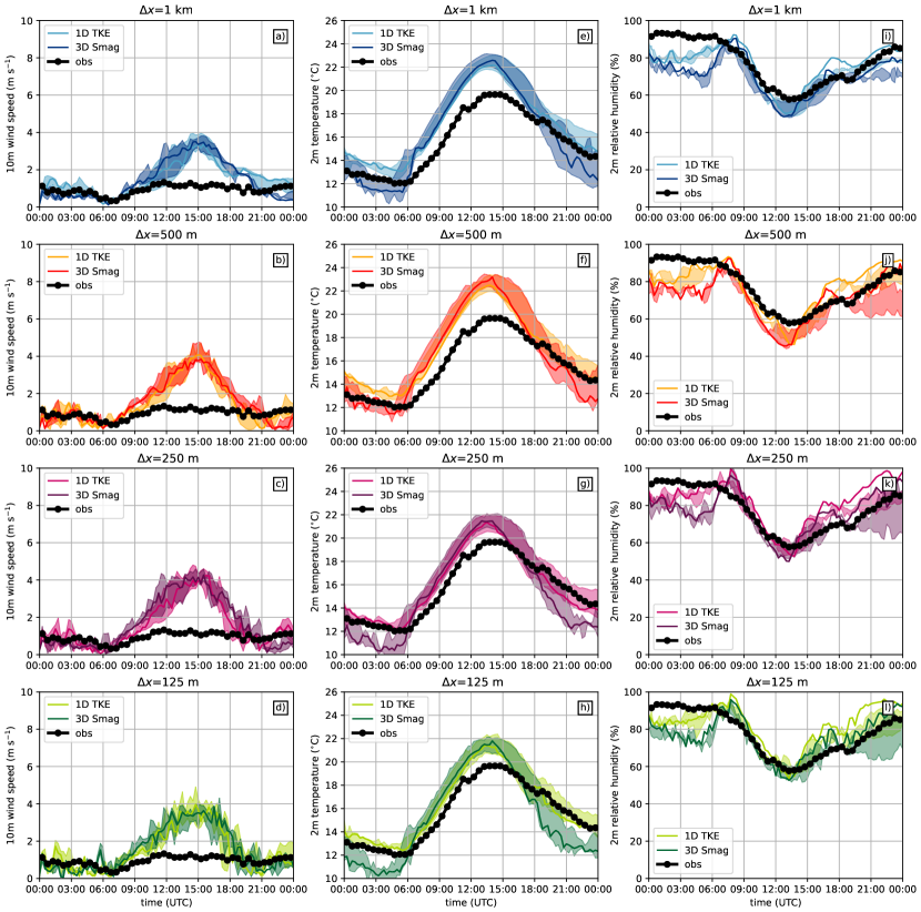
Figure 15: As in Fig. 14, but for the North-facing slope station (CS-NF27).

The North-facing slope station poses a larger challenge for the model to simulate the meteorological variables correctly (Fig. 15). While the 10 m wind speeds are represented well during the night-time, they are overestimated during the daytime, mainly when the up-valley flow is dominating the valley boundary layer (Fig. 15a-d). As discussed in the case study, the overestimation of the horizontal wind speeds is related to the erosion of the slope flows, which are more resilient in reality - and furthermore, the model tends to simulate a too strong up-valley flow, especially at the DX500 and DX250 grid spacings (Fig. 15b,c). Decreasing $\Delta x$ does not seem to have a large positive impact on a successful simulation of 10 m wind speed at the North-facing slope (Fig. 15d).

The correct simulation of 2 m temperature is also a challenge for the model (Fig. 15e-h): Compared to the observations, 2 m temperature is mostly underestimated during the night-time and overestimated during the daytime. Large differences (more than 2 K) emerge between the two turbulence schemes before 06:00 UTC; the 1D TKE scheme generally simulated warmer 2 m temperatures during the down-slope flows at the station. After the up-valley flow phase, the 3D Smagorinsky scheme generally simulates cooler temperatures than in the night before, while the 1D TKE scheme manages to simulate a more accurate 2 m temperature.

For relative humidity (Fig. 15i-l), a similar behaviour is visible as at the valley floor station: The model manages to simulate the diurnal cycle well, where the 3D Smagorinsky scheme generally simulates values in better agreement with the observations during the daytime (after 06:00 UTC until 18:00 UTC), while the 1D TKE scheme performs better during night-time.

A statistical analysis including the calculation of averaged $bias$ and $rmse$ values of the same variables over the five case study days is shown in appendix A.

4 Discussion

4.1 What are the largest challenges for the model for the simulation of the thermally-induced circulation?

Evaluating the model across scales and turbulence schemes at the valley floor revealed a generally good, satisfying performance. However, the simulations at the hectometric range struggle with the correct simulation of the cross-valley vortex due to the Inn Valley’s curvature. While the observations from the co-planar LIDAR scans show a cross-valley vortex with cross-valley flow speed maxima of around 5 m s^-1, the model simulates higher cross-valley flow speeds of around 8 m s^-1, and furthermore, no re-circulation at around 1000 m a.g. is visible. The horizontal extent of the cross-valley circulation is too large compared to the observations. This leads to a too strong influence of the up-valley flow on the North-facing slope station in the model, where the erosion of up-slope flows are eroded. Therefore, this scale interaction between the up-valley flow induced cross-valley vortex and the small-scale up-slope flows at the Northern slope is misrepresented in the model. While we only show the coplanar scans from IOP8, the averaged wind speed time series over all five case study days suggest that this challenge for the model is present for other up-valley flow days as well.

The second large challenge for the model, especially for the 3D Smagorinsky scheme, is the evening transition with the decay of the up-valley flow after 18:00 UTC. Eventually, the wind speed drops in the model, but around 2 hours later compared to observations (and the 1D TKE runs). Again, although the sensible heat fluxes are simulated correctly, the model has a warm bias and positive vertical velocities, preventing the growth of a SBL. This problem is present at the other four case studies as well. The delayed evening transition is related to a too warm CBL in the 3D Smagorinsky runs before noon, leading to a stronger pressure gradient between the valley and the Alpine foreland, favoring the formation of a a stronger up-valley flow. The strong up-valley flow breaks down later than in the observations and the 1D TKE scheme. Strictly speaking, the underlying problem of the 3D Smagorinsky scheme is not the turbulence scheme itself, but the coupled surface transfer scheme, which produced a too high heat exchange during the presence of a CBL. Still, evening transitions in the atmospheric boundary layer are a multi-scale phenomenon [45], and require the correct simulation of the interaction of a smaller scale (the growing SBL) with a larger scale (the decaying up-valley flow). Therefore, we can conclude, that the correct representation of scale interactions likely pose the largest problem for the correct simulation of mountain boundary-layer processes at the hectometric range. The results also show that only increasing the horizontal resolution does not automatically improve the model performance, because many issues remain present across scales.

4.2 Is there an added value in increasing the model resolution?

We performed numerical simulations across the hectometric range for a well-known mountain-boundary layer phenomenon: The thermally-induced up-valley flow circulation in the Inn Valley, Austria. The general diurnal cycle and boundary-layer structure in the valley is simulated well by the DX1000 run, mostly because the valley is already well-resolved at the kilometric range. However, when $\Delta x$ is decreased, small-scale boundary layer features are better resolved: For example, the model warm bias in the nighttime during CAP episodes. In the CBL before noon, DX125 manages to simulate small-scale up- and downdrafts, which are not detectable in coarser simulations. In case of the up-valley flow, the strength of the jet and the daytime wind speed maximum are underestimated for DX1000, while at DX500 and DX250, it is simulated too strongly - together with a too strong cross-valley circulation. This problem is reduced at DX125, but the overestimated cross-valley flow circulation is present at all grid spacings. It has to be mentioned that DX125 is the resolution where the erosion of the small-scale slope flows at the North-facing slope is weakest. The evening transition from up-valley flows back to down-valley flows poses a challenge for the model - however, also in this case, a smaller grid spacing yields the best results in terms of wind speed and direction. The added value of higher horizontal resolution – even when keeping the vertical resolution constant – is especially given when smaller scales start to become relevant, e.g. for cold-air pools or the evening transition, which in turn also leads to a better representation of scale interactions. However, although higher resolution leads to the aforementioned improvements, it still has to be discussed whether it justifies the increased usage of computational resources. If the biases are reduced – e.g., by improving the model physics – the increased computational resources due to higher resolution become more justifiable for operational NWP.

4.3 At which horizontal grid spacing should we switch to a 3D turbulence scheme?

Surprisingly, the performance of the two turbulence schemes was similar through most of the simulation time. The reason for this unexpected behavior is the model’s inability to appropriately capture the interaction between the small scales generated by the surface heterogeneity and the background large-scale flow. We also have to mention that we did not tune the 3D Smagorinsky scheme and ran it with the “default settings". Therefore, it can expected that improvements with the scheme are possible after a more systematic analysis of scheme and the accompanying tuning. However, judging from the general meteorological variables, both schemes deliver a satisfactory performance during our five case study days. Differences between the schemes were detectable in the up-valley flow onset and especially during the evening transition, which is delayed in the 3D Smagorinsky scheme. Judging from these results, the surface layer scheme has a larger impact on the correct simulation of the valley boundary layer than the turbulence scheme. This is in agreement with the findings of [66], who noticed after a model intercomparison on valley winds, that the largest discrepancies between the models emerged due to the different parameterizations of the soil-surface-atmosphere interactions. [79] argue as well that the representation of the underlying surface is more relevant for a successful mountain boundary layer simulation than the choice of the turbulence scheme. Our study now confirms the findings of these two idealized numerical studies with real-case simulations.

We have not yet reached the range where a 1D TKE parameterization completely fails with our current set-up - therefore, both our tested schemes are applicable to the hectometric range. We cautiously conclude, in agreement with [57], that at grid spacings below 100 m a 1D PBL parameterization should be avoided. However, in our simulations at the hectometric range, we have not yet explored the simulated turbulence structure across schemes and grid spacings in much detail - this will be subject for a future study.

5 Conclusions and Outlook

In this study, we investigated the performance of the ICON model across four horizontal grid spacings ($\Delta x=1$ km, $\Delta x=500$ m, $\Delta x=250$ m, and $\Delta x=125$ m) for the simulation of the mountain boundary layer in the Inn Valley, Austria. Furthermore, we employed two available turbulence schemes - a 1D boundary-layer parameterization (1D TKE) and a 3D LES closure (3D Smagorinsky) to assess the performance of the two schemes across resolutions. For model validation, we utilized LIDAR scans (vertical profiles and cross-valley scans) from the CROSSINN measurement campaign and point observations from the i-Box turbulence flux towers. We simulated five case studies of days in summer/autumn of 2019, where a thermally-induced circulation with up-valley flows is present, and we analyzed one case study in particular, where radiosonde observations are available as well (September 13, 2019 – IOP8). The results allow us to draw the following conclusions:

1. Generally speaking, the model is successful in simulating the valley boundary layer structure across horizontal grid spacings and turbulence schemes, because it can be assumed that the Inn Valley is already well-resolved at the hectometric range.

2. At the kilometric range, the wind speeds associated with the up-valley flow are underestimated. This problem is less pronounced in the simulation with the 3D Smagorinsky scheme, likely due to the contribution of horizontal shear production.

3. At the hectometric change, wind speeds tend to be overestimated by the model, which might be related to a double-counting problem in the turbulence grey zone.

4. The simulations with the smallest grid spacing ($\Delta x=125$ m) show a realistic simulation of the thermal structure of the valley boundary layer, especially for the representation of cold-air pools, the multiple inversions in the valley boundary layer, and up-valley flow speeds.

5. During most of the simulation time, there are no large differences between the two tested turbulence schemes in the simulation of the valley boundary layer. The exception is the evening transition, where the 3D Smagorinsky scheme simulates a delayed decay of the up-valley flow. This is mostly related to the two different surface layer schemes coupled to the turbulence schemes, leasing to a too warm valley atmosphere before noon and henceforth the buildup of a stronger pressure gradient between valley and surrounding foreland, leading to stronger up-valley flows win the 3D Smagorinsky scheme simulation.

6. The model is able to simulate the spatial variability of the valley boundary layer, although the model tends to simulate to too strong cross-valley circulation, leading to the erosion of small-scale slope flows at the North-facing slope.

7. The largest challenge for the model remains the interactions between larger and smaller scales, manifested in the erosion of up-slope flows by the larger-scale up-valley flow and the prevented growth of a stable boundary layer after the up-valley flow breaks down. This problem remains across all tested horizontal grid spacings.

This study aimed to give an overview whether simply increasing the horizontal resolution yields better model results. The findings agree that the lower boundary condition - namely, the better-resolved topography - mainly governs the boundary-layer flow. However, challenges remain also at the highest resolution, mostly related to scale interactions which are common in complex topography. The CROSSINN observations provide a valuable data pool for a detailed model evaluation for the valley cross-section. However, our model evaluation is very localized and still limited to the lower Inn Valley. We will extend the analysis of our simulation dataset, mostly by exploring the turbulence representation in the model across scales. In the near future, multi-dimensional observations – also along the valley – will be necessary to further explore the model performance in complex terrain. For this purpose, the future TEAMx measurement campaigns [61] will provide valuable observations of the mountain boundary layer.

conflict of interest

The authors declare no conflict of interest.

data availability

Observational data stem from the CROSSINN campaign [3]. The SL88 and SLXR 142 LIDAR data were retrieved from [24]. The coplanar LIDAR scans and radiosonde data were downloaded from [1, 2]. The post-processed turbulence flux tower data from the i-Box stations can be retrieved at https://acinn-data.uibk.ac.at/.

We used the ICON model code version 2.6.5 for our simulations. The model code can be obtained by following the guidelines at https://code.mpimet.mpg.de/projects/iconpublic/wiki/How%20to%20obtain%20the%20model%20code. The native ICON grid was re-interpolated to latitude/longitude coordinates with the Climate Data Operators tool (CDO, https://code.mpimet.mpg.de/projects/cdo). The model namelists and the python scripts for model post-processing are available at [20]. Figures were generated with python-matplotlib [35] using colormaps by [13].

Appendix A BIAS and RMSE table

Table A1 shows the calculated model validation statistics for the valley floor station (CS-VF0) and the North-facing slope (CS-NF27) over the five case study days. Bias and rmse were obtained as follows:

$$bias=\frac{1}{N_{t}}\sum^{N_{t}}_{i=1}{{M_{i}-O_{i}}}$$ (1)

and

$$rmse=\left(\frac{1}{N_{t}}\sum^{N_{t}}_{i=1}{(M_{i}-O_{i})}^{2}\right)^{\frac{1}{2}},$$ (2)

where $M_{i}$ is the median of the five case study days, $O_{i}$ are the i-Box observations, and $N_{t}=5$ are the number of case study days.

Variable	Location	DX	$bias$ 1D TKE	$rmse$ 1D TKE	$bias$ 3D Smag	$rmse$ 3D Smag
T 2 m	CS-VF0	1000 m	0.018	1.61	-0.548	1.030
	CS-NF27	1000 m	1.523	0.798	0.798	1.489
	CS-VF0	500 m	0.126	1.450	0.0120	0.957
	CS-NF27	500 m	1.383	1.573	1.059	1.664
	CS-VF0	250 m	-0.075	1.135	0.277	1.184
	CS-NF27	250 m	0.487	0.843	-0.127	1.296
	CS-VF0	125 m	-0.129	1.204	0.181	1.128
	CS-NF27	125 m	0.626	0.874	-0.232	1.370
U 10 m	CS-VF0	1000 m	0.574	1.511	0.651	1.442
	CS-NF27	1000 m	0.485	0.817	0.382	0.892
	CS-VF0	500 m	1.047	2.214	1.257	2.104
	CS-NF27	500 m	0.460	1.044	0.504	1.115
	CS-VF0	250 m	1.033	2.170	1.541	2.523
	CS-NF27	250 m	0.565	1.147	0.626	1.263
	CS-VF0	125 m	0.917	2.010	1.365	2.262
	CS-NF27	125 m	0.469	1.032	0.424	0.993
RH 2 m	CS-VF0	1000 m	-2.896	6.829	-7.819	10.199
	CS-NF27	1000 m	15.910	16.807	12.257	13.436
	CS-VF0	500 m	-2.651	7.135	-7.939	8.926
	CS-NF27	500 m	14.759	15.720	9.280	10.681
	CS-VF0	250 m	0.504	7.498	-6.314	7.612
	CS-NF27	250 m	16.225	17.374	9.968	11.522
	CS-VF0	125 m	0.917	2.010	1.365	2.262
	CS-NF27	125 m	16.814	17.925	10.516	11.920

Table 2: Bias and Rmse, averaged over five case study days.

References

- Adler et al. [2021a] Adler, B., Babić, N., Kalthoff, N. and Wieser, A. (2021a) CROSSINN (cross-valley flow in the Inn Valley investigated by dual-Doppler lidar measurements) - KITcube data sets [CHM 15k, GRAW, HATPRO2, Mobotix, Photos].
- Adler et al. [2021b] — (2021b) CROSSINN (Cross-valley flow in the Inn Valley investigated by dual-Doppler lidar measurements) - KITcube data sets [WLS200s].
- Adler et al. [2021c] Adler, B., Gohm, A., Kalthoff, N., Babić, N., Corsmeier, U., Lehner, M., Rotach, M. W., Haid, M., Markmann, P., Gast, E., Tsaknakis, G. and Georgoussis, G. (2021c) CROSSINN: A field experiment to study the three-dimensional flow structure in the Inn Valley, Austria. Bull. Amer. Meteorol. Soc., 102, E38 – E60.
- Adler et al. [2023a] Adler, B., Wilczak, J. M., Bianco, L., Bariteau, L., Cox, C. J., de Boer, G., Djalalova, I. V., Gallagher, M. R., Intrieri, J. M., Meyers, T. P., Myers, T. A., Olson, J. B., Pezoa, S., Sedlar, J., Smith, E., Turner, D. D. and White, A. B. (2023a) Impact of seasonal snow-cover change on the observed and simulated state of the atmospheric boundary layer in a high-altitude mountain valley. J. Geophys. Res. Atmos., 128, e2023JD038497.
- Adler et al. [2023b] Adler, B., Wilczak, J. M., Kenyon, J., Bianco, L., Djalalova, I. V., Olson, J. B. and Turner, D. D. (2023b) Evaluation of a cloudy cold-air pool in the columbia river basin in different versions of the high-resolution rapid refresh (hrrr) model. Geosci Model Dev, 16, 597–619.
- Babić et al. [2021] Babić, N., Adler, B., Gohm, A., Kalthoff, N., Haid, M., Lehner, M., Ladstätter, P. and Rotach, M. W. (2021) Cross-valley vortices in the Inn valley, Austria: Structure, evolution and governing force imbalances. Q. J. R. Meteorol. Soc., 147, 3835–3861.
- Bauer et al. [2023] Bauer, H.-S., Späth, F., Lange, D., Thundathil, R., Ingwersen, J., Behrendt, A. and Wulfmeyer, V. (2023) Evolution of the convective boundary layer in a WRF simulation nested down to 100 m resolution during a cloud-free case of LAFE, 2017 and comparison to observations. J. Geophys.Res. Atmos., 128, e2022JD037212.
- Bauer et al. [2015] Bauer, P., Thorpe, A. and Brunet, G. (2015) The quiet revolution of numerical weather prediction. Nature, 525, 47–55.
- Buzzi [2008] Buzzi, M. (2008) Challenges in Operational Wintertime Weather Prediction at High Resolution in Complex Terrain. Ph.D. thesis, ETH Zürich.
- Buzzi et al. [2011] Buzzi, M., Rotach, M. W., Raschendorfer, M. and Holtslag, A. A. M. (2011) Evaluation of the COSMO-SC turbulence scheme in a shear-driven stable boundary layer. Meteor. Z., 20, 335–350.
- Chow et al. [2019] Chow, F. K., Schär, C., Ban, N., Lundquist, K. A., Schlemmer, L. and Shi, X. (2019) Crossing multiple gray zones in the transition from mesoscale to microscale simulation over complex terrain. Atmosphere, 10.
- Chow et al. [2006] Chow, F. K., Weigel, A. P., Street, R. L., Rotach, M. W. and Xue, M. (2006) High-Resolution Large-Eddy Simulations of Flow in a Steep Alpine Valley. Part I: Methodology, Verification, and Sensitivity Experiments. J. Appl. Meteor. Climatol., 45, 63–86.
- Crameri [2023] Crameri, F. (2023) Scientific colour maps.
- Cuxart [2015] Cuxart, J. (2015) When Can a High-Resolution Simulation Over Complex Terrain be Called LES? Front. Earth Sci., 3, 6.
- Dipankar et al. [2015] Dipankar, A., Stevens, B., Heinze, R., Moseley, C., Zängl, G., Giorgetta, M. and Brdar, S. (2015) Large eddy simulation using the general circulation model ICON. J Adv Model Earth Sys, 7, 963–986.
- Efstathiou and Beare [2015] Efstathiou, G. A. and Beare, R. J. (2015) Quantifying and improving sub-grid diffusion in the boundary-layer grey zone. Q. J. R. Meteorol. Soc., 141, 3006–3017.
- European Environmental Agency [2017] European Environmental Agency (2017) Copernicus Land Service — Pan-European Component: CORINE Land Cover. URL: http://land.copernicus.eu/pan-european/corine-land-cover/clc-2012.
- FAO/IIASA/ISSCAS/JRC [2012] FAO/IIASA/ISSCAS/JRC (2012) Harmonized World Soil Database (version 1.2). FAO, Rome, Italy and IIASA, Laxenburg, Austria. [Available online at http://webarchive.iiasa.ac.at/Research/LUC/External-World-soil-database/HTML/].
- Gerber et al. [2018] Gerber, F., Besic, N., Sharma, V., Mott, R., Daniels, M., Gabella, M., Berne, A., Germann, U. and Lehning, M. (2018) Spatial variability in snow precipitation and accumulation in COSMO–WRF simulations and radar estimations over complex terrain. The Cryosphere, 12, 3137–3160.
- Goger [2023] Goger, B. (2023) Modelling the mountain boundary layer at the hectometric range - ICON Namelists and Python Scripts.
- Goger et al. [2018] Goger, B., Rotach, M. W., Gohm, A., Fuhrer, O., Stiperski, I. and Holtslag, A. A. M. (2018) The impact of three-dimensional effects on the simulation of turbulence kinetic energy in a major alpine valley. Boundary-Layer Meteorol, 168, 1–27.
- Goger et al. [2019] Goger, B., Rotach, M. W., Gohm, A., Stiperski, I., Fuhrer, O. and de Morsier, G. (2019) A new horizontal length scale for a three-dimensional turbulence parameterization in mesoscale atmospheric modeling over highly complex terrain. J. Appl. Meteor. Climatol., 58, 2087–2102.
- Goger et al. [2022] Goger, B., Stiperski, I., Nicholson, L. and Sauter, T. (2022) Large-eddy simulations of the atmospheric boundary layer over an alpine glacier: Impact of synoptic flow direction and governing processes. Q. J. R. Meteorol. Soc, 148, 1319–1343.
- Gohm et al. [2021] Gohm, A., Haid, M. and Rotach, M. W. (2021) CROSSINN (Cross-valley flow in the Inn Valley investigated by dual-Doppler lidar measurements) - ACINN Doppler wind lidar data sets (SL88, SLXR142).
- Gohm et al. [2004] Gohm, A., Zängl, G. and Mayr, G. J. (2004) South Foehn in the Wipp Valley on 24 October 1999 (MAP IOP 10): Verification of High-Resolution Numerical Simulations with Observations. Mon. Wea. Rev., 132, 78–102.
- Golzio et al. [2021] Golzio, A., Ferrarese, S., Cassardo, C., Diolaiuti, G. A. and Pelfini, M. (2021) Land-use improvements in the weather research and forecasting model over complex mountainous terrain and comparison of different grid sizes. Boundary-Layer Meteorol., 180, 319–351.
- Haid et al. [2020] Haid, M., Gohm, A., Umek, L., Ward, H. C., Muschinski, T., Lehner, L. and Rotach, M. W. (2020) Foehn-cold pool interactions in the Inn Valley during PIANO IOP2. Q. J. R. Meteorol. Soc., 146, 1232–1263.
- Haiden et al. [2018] Haiden, T., Sandu, I., Balsamo, G., Arduini, G. and Beljaars, A. (2018) Addressing biases in near-surface forecasts. ECMWF Newsletter. URL: https://www.ecmwf.int/en/newsletter/157/meteorology/addressing-biases-near-surface-forecasts.
- Heinze et al. [2017] Heinze, R., Dipankar, A., Carbajal Henken, C., Moseley, C., Sourdeval, O., Trömel, S., Xie, X., Adamidis, P., Ament, F., Baars, H., Barthlott, C., Behrendt, A., Blahak, U., Bley, S., Brdar, S., Brueck, M., Crewell, S., Deneke, H., Di Girolamo, P., Evaristo, R., Fischer, J., Frank, C., Friederichs, P., Göcke, T., Gorges, K., Hande, L., Hanke, M., Hansen, A., Hege, H.-C., Hoose, C., Jahns, T., Kalthoff, N., Klocke, D., Kneifel, S., Knippertz, P., Kuhn, A., van Laar, T., Macke, A., Maurer, V., Mayer, B., Meyer, C. I., Muppa, S. K., Neggers, R. A. J., Orlandi, E., Pantillon, F., Pospichal, B., Röber, N., Scheck, L., Seifert, A., Seifert, P., Senf, F., Siligam, P., Simmer, C., Steinke, S., Stevens, B., Wapler, K., Weniger, M., Wulfmeyer, V., Zängl, G., Zhang, D. and Quaas, J. (2017) Large-eddy simulations over Germany using ICON: A comprehensive evaluation. Q. J. R. Meteorol. Soc., 143, 69–100.
- Hogan and Bozzo [2016] Hogan, R. and Bozzo, A. (2016) ECRAD: A new radiation scheme for the IFS.
- Hohenegger et al. [2023] Hohenegger, C., Korn, P., Linardakis, L., Redler, R., Schnur, R., Adamidis, P., Bao, J., Bastin, S., Behravesh, M., Bergemann, M., Biercamp, J., Bockelmann, H., Brokopf, R., Brüggemann, N., Casaroli, L., Chegini, F., Datseris, G., Esch, M., George, G., Giorgetta, M., Gutjahr, O., Haak, H., Hanke, M., Ilyina, T., Jahns, T., Jungclaus, J., Kern, M., Klocke, D., Kluft, L., Kölling, T., Kornblueh, L., Kosukhin, S., Kroll, C., Lee, J., Mauritsen, T., Mehlmann, C., Mieslinger, T., Naumann, A. K., Paccini, L., Peinado, A., Praturi, D. S., Putrasahan, D., Rast, S., Riddick, T., Roeber, N., Schmidt, H., Schulzweida, U., Schütte, F., Segura, H., Shevchenko, R., Singh, V., Specht, M., Stephan, C. C., von Storch, J.-S., Vogel, R., Wengel, C., Winkler, M., Ziemen, F., Marotzke, J. and Stevens, B. (2023) ICON-Sapphire: simulating the components of the earth system and their interactions at kilometer and subkilometer scales. Geosci Model Dev, 16, 779–811.
- Honnert et al. [2020] Honnert, R., Efstathiou, G. A., Beare, R. J., Ito, J., Lock, A., Neggers, R., Plant, R. S., Shin, H. H., Tomassini, L. and Zhou, B. (2020) The atmospheric boundary layer and the "gray zone" of turbulence: A critical review. J. Geophys. Res. Atmos., 125, e2019JD030317.
- Honnert and Masson [2014] Honnert, R. and Masson, V. (2014) What is the smallest physically acceptable scale for 1D turbulence schemes? Front. Earth Sci., 2, 5.
- Honnert et al. [2011] Honnert, R., Masson, V. and Couvreux, F. (2011) A Diagnostic for Evaluating the Representation of Turbulence in Atmospheric Models at the Kilometric Scale. J. Atmos. Sci., 68, 3112–3131.
- Hunter [2007] Hunter, J. D. (2007) Matplotlib: A 2D Graphics Environment. Comput. Sci. & Eng., 9, 90–95.
- Juliano et al. [2022] Juliano, T. W., Kosović, B., Jiménez, P. A., Eghdami, M., Haupt, S. E. and Martilli, A. (2022) “Gray zone” simulations using a three-dimensional planetary boundary layer parameterization in the weather research and forecasting model. Mon Wea Rev, 150, 1585 – 1619.
- Kalverla et al. [2016] Kalverla, P. C., Duine, G.-J., Steeneveld, G.-J. and Hedde, T. (2016) Evaluation of the Weather Research and Forecasting Model in the Durance Valley Complex Terrain during the KASCADE Field Campaign. J. Appl. Meteor. Climatol., 55, 861–882.
- Lehner and Rotach [2018] Lehner, M. and Rotach, M. W. (2018) Current challenges in understanding and predicting transport and exchange in the atmosphere over mountainous terrain. Atmosphere, 9, 28.
- Lehner et al. [2019] Lehner, M., Rotach, M. W. and Obleitner, F. (2019) A method to identify synoptically undisturbed, clear-sky conditions for valley-wind analysis. Boundary-Layer Meteorol., 173, 435–450.
- Lehner et al. [2021] Lehner, M., Rotach, M. W., Sfyri, E. and Obleitner, F. (2021) Spatial and temporal variations in near-surface energy fluxes in an alpine valley under synoptically undisturbed and clear-sky conditions. Q. J. R. Meteorol. Soc., 147, 2173–2196.
- Leuenberger et al. [2010] Leuenberger, D., Koller, M., Fuhrer, O. and Schär, C. (2010) A Generalization of the SLEVE Vertical Coordinate. Mon. Wea. Rev., 138, 3683–3689.
- Leutwyler et al. [2016] Leutwyler, D., Fuhrer, O., Lapillonne, X., Lüthi, D. and Schär, C. (2016) Towards European-scale convection-resolving climate simulations with GPUs: a study with COSMO 4.19. Geosci. Model Dev., 9, 3393–3412.
- Lilly [1962] Lilly, D. K. (1962) On the numerical simulation of buoyant convection. Tellus, 14, 148–172.
- Liu et al. [2020] Liu, Y., Liu, Y., Muñoz Esparza, D., Hu, F., Yan, C. and Miao, S. (2020) Simulation of Flow Fields in Complex Terrain with WRF-LES: Sensitivity Assessment of Different PBL Treatments. J. Appl. Meteor. Climatol., 59, 1481–1501.
- Lothon et al. [2014] Lothon, M., Lohou, F., Pino, D., Couvreux, F., Pardyjak, E. R., Reuder, J., Vilà -Guerau de Arellano, J., Durand, P., Hartogensis, O., Legain, D., Augustin, P., Gioli, B., Lenschow, D. H., Faloona, I., Yagüe, C., Alexander, D. C., Angevine, W. M., Bargain, E., Barrié, J., Bazile, E., Bezombes, Y., Blay-Carreras, E., van de Boer, A., Boichard, J. L., Bourdon, A., Butet, A., Campistron, B., de Coster, O., Cuxart, J., Dabas, A., Darbieu, C., Deboudt, K., Delbarre, H., Derrien, S., Flament, P., Fourmentin, M., Garai, A., Gibert, F., Graf, A., Groebner, J., Guichard, F., Jiménez, M. A., Jonassen, M., van den Kroonenberg, A., Magliulo, V., Martin, S., Martinez, D., Mastrorillo, L., Moene, A. F., Molinos, F., Moulin, E., Pietersen, H. P., Piguet, B., Pique, E., Román-Cascón, C., Rufin-Soler, C., Saïd, F., Sastre-Marugán, M., Seity, Y., Steeneveld, G. J., Toscano, P., Traullé, O., Tzanos, D., Wacker, S., Wildmann, N. and Zaldei, A. (2014) The BLLAST field experiment: Boundary-Layer Late Afternoon and Sunset Turbulence. Atmos. Chem. Phys., 14, 10931–10960.
- Louis [1979] Louis, J.-F. (1979) A parametric model of vertical eddy fluxes in the atmosphere. Boundary-Layer Meteorol., 17, 187–202.
- Mauder et al. [2020] Mauder, M., Foken, T. and Cuxart, J. (2020) Surface-energy-balance closure over land: A review. Boundary Layer Meteorol., 177, 395–426.
- Mellor and Yamada [1974] Mellor, G. L. and Yamada, T. (1974) A Hierarchy of Turbulence Closure Models for Planetary Boundary Layers. J. Atmos. Sci., 31, 1791–1806.
- Mellor and Yamada [1982] — (1982) Development of a turbulence closure model for geophysical fluid problems. Rev. Geophys., 20, 851–875.
- Mikkola et al. [2023] Mikkola, J., Sinclair, V. A., Bister, M. and Bianchi, F. (2023) Daytime along-valley winds in the Himalayas as simulated by the weather research and forecasting (WRF) model. Atmos. Chem. Phys., 23, 821–842.
- Mironov et al. [2010] Mironov, D., Heise, E., Kourzeneva, E., Ritter, B., Schneider, S. and Terzhevik, A. (2010) Implementation of the lake parameterisation scheme flake into the numerical weather prediction model COSMO. Boreal Env. Res., 15, 97–99. URL: https://www.borenv.net/BER/archive/ber152.htm.
- Miyamoto et al. [2013] Miyamoto, Y., Kajikawa, Y., Yoshida, R., Yamaura, T., Yashiro, H. and Tomita, H. (2013) Deep moist atmospheric convection in a subkilometer global simulation. Geophys Res Lett, 40, 4922–4926.
- Muñoz-Esparza et al. [2014] Muñoz-Esparza, D., Kosović, B., Mirocha, J. and Beeck, J. v. (2014) Bridging the Transition from Mesoscale to Microscale Turbulence in Numerical Weather Prediction Models. Boundary-Layer Meteorol., 153, 409–440.
- Muńoz-Esparza et al. [2017] Muńoz-Esparza, D., Lundquist, J. K., Sauer, J. A., Kosović, B. and Linn, R. R. (2017) Coupled mesoscale-les modeling of a diurnal cycle during the CWEX-13 field campaign: From weather to boundary-layer eddies. J. Adv. Model. Earth Syst., 9, 1572–1594.
- NASA/METI/AIST/Japan Spacesystems and U.S./Japan ASTER Science Team [2009] NASA/METI/AIST/Japan Spacesystems and U.S./Japan ASTER Science Team (2009) ASTER Global Digital Elevation Model. NASA EOSDIS Land Processes DAAC.
- Prill et al. [2022] Prill, F., Reinert, D., Rieger, D. and Zängl, G. (2022) Working with the ICON model.
- Rai et al. [2019] Rai, R. K., Berg, L. K., Kosović, B., Haupt, S. E., Mirocha, J. D., Ennis, B. L. and Draxl, C. (2019) Evaluation of the impact of horizontal grid spacing in terra incognita on coupled mesoscale–microscale simulations using the WRF framework. Mon Wea Rev, 147, 1007 – 1027.
- Raschendorfer [2001] Raschendorfer, M. (2001) The new turbulence parameterization of LM. COSMO Newsletter, 1, 89–98. URL: http://www.cosmo-model.org/content/model/documentation/newsLetters/newsLetter01/newsLetter_01.pdf.
- Rihani et al. [2015] Rihani, J. F., Chow, F. K. and Maxwell, R. M. (2015) Isolating effects of terrain and soil moisture heterogeneity on the atmospheric boundary layer: Idealized simulations to diagnose land-atmosphere feedbacks. J. Adv. Model. Earth Syst., 7, 915–937.
- Rotach et al. [2008] Rotach, M. W., Andretta, M., Calanca, P., Weigel, A. and Weiss, A. (2008) Boundary layer characteristics and turbulent exchange mechanisms in highly complex terrain. Acta Geophys., 56, 194–219.
- Rotach et al. [2022] Rotach, M. W., Serafin, S., Ward, H. C., Arpagaus, M., Colfescu, I., Cuxart, J., Wekker, S. F. J. D., Grubišic, V., Kalthoff, N., Karl, T., Kirshbaum, D. J., Lehner, M., Mobbs, S., Paci, A., Palazzi, E., Bailey, A., Schmidli, J., Wittmann, C., Wohlfahrt, G. and Zardi, D. (2022) A collaborative effort to better understand, measure, and model atmospheric exchange processes over mountains. Bull Amer Meteorol Soc, 103, E1282 – E1295.
- Rotach et al. [2017] Rotach, M. W., Stiperski, I., Fuhrer, O., Goger, B., Gohm, A., Obleitner, F., Rau, G., Sfyri, E. and Vergeiner, J. (2017) Investigating Exchange Processes over Complex Topography: The Innsbruck Box (i-Box). Bull. Amer. Meteor. Soc., 98, 787–805.
- Rotach et al. [2014] Rotach, M. W., Wohlfahrt, G., Hansel, A., Reif, M., Wagner, J. and Gohm, A. (2014) The World is Not Flat: Implications for the Global Carbon Balance. Bull. Amer. Meteor. Soc., 95, 1021–1028.
- Schär et al. [2020] Schär, C., Fuhrer, O., Arteaga, A., Ban, N., Charpilloz, C., Di Girolamo, S., Hentgen, L., Hoefler, T., Lapillonne, X., Leutwyler, D., Osterried, K., Panosetti, D., Rüdisühli, S., Schlemmer, L., Schulthess, T. C., Sprenger, M., Ubbiali, S. and Wernli, H. (2020) Kilometer-Scale Climate Models: Prospects and Challenges. Bull. Amer. Meteor. Soc., 101, E567–E587.
- Schmidli [2013] Schmidli, J. (2013) Daytime Heat Transfer Processes over Mountainous Terrain. J. Atmos. Sci., 70, 4041–4066.
- Schmidli et al. [2010] Schmidli, J., Billings, B., Chow, F. K., de Wekker, S. F. J., Doyle, J., Grubišić, V., Holt, T., Jiang, Q., Lundquist, K. A., Sheridan, P., Vosper, S., Whiteman, C. D., Wyszogrodzki, A. A. and Zängl, G. (2010) Intercomparison of Mesoscale Model Simulations of the Daytime Valley Wind System. Mon. Wea. Rev., 139, 1389–1409.
- Schmidli et al. [2018] Schmidli, J., Böing, S. and Fuhrer, O. (2018) Accuracy of simulated diurnal valley winds in the Swiss Alps: Influence of grid resolution, topography filtering, and land surface datasets. Atmosphere, 9, 196.
- Schmidli and Quimbayo-Duarte [2023] Schmidli, J. and Quimbayo-Duarte, J. (2023) Diurnal valley winds in a deep alpine valley: Model results. Meteorology, 2, 87–106.
- Schulz and Vogel [2020] Schulz, J.-P. and Vogel, G. (2020) Improving the processes in the land surface scheme terra: Bare soil evaporation and skin temperature. Atmosphere, 11, 513.
- Serafin et al. [2018] Serafin, S., Adler, B., Cuxart, J., De Wekker, S. F. J., Gohm, A., Grisogono, B., Kalthoff, N., Kirshbaum, D. J., Rotach, M. W., Schmidli, J., Stiperski, I., Večenaj, Ž. and Zardi, D. (2018) Exchange processes in the atmospheric boundary layer over mountainous terrain. Atmosphere, 9, 102.
- Serafin and Zardi [2010] Serafin, S. and Zardi, D. (2010) Structure of the Atmospheric Boundary Layer in the Vicinity of a Developing Upslope Flow System: A Numerical Model Study. J. Atmos. Sci., 67, 1171–1185.
- Singh et al. [2021] Singh, S., Kalthoff, N. and Gantner, L. (2021) Sensitivity of convective precipitation to model grid spacing and land-surface resolution in ICON. Q. J. R. Meteorol. Soc., 147, 2709–2728.
- Smagorinsky [1963] Smagorinsky, J. (1963) General circulation experiments with the primitive equations. Mon. Wea. Rev., 91, 99–164.
- Stevens et al. [2020] Stevens, B., Aquistapache, C., Hansen, A., Heinze, R., Klinger, C., Klocke, D., Rybka, H., Schubotz, W., Windmiller, J., Adamidis, P., Arka, I., Barlakas, V., Biercamp, J., Brueck, M., Brune, S., Buehler, S. A., Burkhardt, U., Cioni, G., Costa-Surós, M., Crewell, S., Crüger, T., Deneke, H., Friedrichs, P., Henken, C. C., Hohenegger, C., Jacob, M., Jakub, F., Kalthoff, N., Köhler, M., van Laar, T. W., Li, P., Löhnert, U., Macke, A., Madenach, N., Mayer, B., Nam, C., Naumann, A. K., Peters, K., Poll, S., Quaas, J., Röber, N., Rochetin, N., Scheck, L., Schemann, V., Schnitt, S., Seifert, A., Senf, F., Shapkalijewski, M., Simmer, C., Singh, S., Sourdeval, O., Spickermann, D., Strandgren, J., Tessiot, O., Vercauteren, N., Vial, J., Voigt, A. and Zängl, G. (2020) The added value of large-eddy and storm-resolving models for simulating clouds and precipitation. J. Meteorol. Soc. Japan Ser. II, 98, 395–435.
- Stiperski and Calaf [2023] Stiperski, I. and Calaf, M. (2023) Generalizing Monin-Obukhov similarity theory (1954) for complex atmospheric turbulence. Phys. Rev. Lett., 130, 124001.
- Umek et al. [2021] Umek, L., Gohm, A., Haid, M., Ward, H. C. and Rotach, M. W. (2021) Large eddy simulation of foehn-cold pool interactions in the Inn Valley during PIANO IOP2. Q. J. R. Meteor. Soc., 147, 944–982.
- Umek et al. [2022] — (2022) Influence of grid resolution of large-eddy simulations on foehn-cold pool interaction. Q. J. R. Meteorol. Soc., 148, 1840–1863.
- Vergeiner and Dreiseitl [1987] Vergeiner, I. and Dreiseitl, E. (1987) Valley winds and slope winds — Observations and elementary thoughts. Meteorol. Atmos. Phys., 36, 264–286.
- Wagner et al. [2014] Wagner, J. S., Gohm, A. and Rotach, M. W. (2014) The Impact of Horizontal Model Grid Resolution on the Boundary Layer Structure over an Idealized Valley. Mon. Wea. Rev., 142, 3446–3465.
- Wagner et al. [2015] — (2015) The impact of valley geometry on daytime thermally driven flows and vertical transport processes. Q. J. R. Meteorol. Soc., 141, 1780–1794.
- Weigel et al. [2006] Weigel, A. P., Chow, F. K., Rotach, M. W., Street, R. L. and Xue, M. (2006) High-Resolution Large-Eddy Simulations of Flow in a Steep Alpine Valley. Part II: Flow Structure and Heat Budgets. J. Appl. Meteor. Climatol., 45, 87–107.
- Weigel and Rotach [2004] Weigel, A. P. and Rotach, M. W. (2004) Flow structure and turbulence characteristics of the daytime atmosphere in a steep and narrow Alpine valley. Q. J. R. Meteorol. Soc., 130, 2605–2627.
- Wyngaard [2004] Wyngaard, J. C. (2004) Toward Numerical Modeling in the “Terra Incognita”. J. Atmos. Sci., 61, 1816–1826.
- Zhang et al. [2018] Zhang, X., Bao, J.-W., Chen, B. and Grell, E. D. (2018) A Three-Dimensional Scale-Adaptive Turbulent Kinetic Energy Scheme in the WRF-ARW Model. Mon. Wea. Rev., 146, 2023–2045.
- Zhong and Chow [2013] Zhong, S. and Chow, F. K. (2013) Meso- and Fine-Scale Modeling over Complex Terrain: Parameterizations and Applications. In Mountain Weather Research and Forecasting (eds. F. K. Chow, S. F. J. De Wekker and B. J. Snyder), Springer Atmospheric Sciences, 591–653. Springer Netherlands.
- Zhou et al. [2014] Zhou, B., Simon, J. S. and Chow, F. K. (2014) The Convective Boundary Layer in the Terra Incognita. J. Atmos. Sci., 71, 2545–2563.
- Zängl [2012] Zängl, G. (2012) Extending the numerical stability limit of terrain-following coordinate models over steep slopes. Mon Wea Rev, 140, 3722 – 3733.
- Zängl et al. [2015] Zängl, G., Reinert, D., Rípodas, P. and Baldauf, M. (2015) The ICON (ICOsahedral Non-hydrostatic) modelling framework of DWD and MPI-M: Description of the non-hydrostatic dynamical core. Q J R Meteorol Soc, 141, 563–579.