The expansion of the GRB 221009A afterglow

We observed $\upgamma$-ray burst (GRB) 221009A using Very Long Baseline Interferomety (VLBI) with the European VLBI Network (EVN) and the Very Long Baseline Array (VLBA), over a period spanning from 40 to 262 days after the initial GRB. The high angular resolution ($\sim$mas) of our observations allowed us, for the second time ever after GRB 030329, to measure the projected size, $s$, of the relativistic shock caused by the expansion of the GRB ejecta into the surrounding medium. Our observations support the expansion of the shock with a 3.6 $\sigma$-equivalent significance, and confirm its relativistic nature by revealing an apparently superluminal expansion rate. Fitting a power law expansion model, $s\propto t^{a}$, to the observed size evolution, we find a slope $a=1.9_{-0.6}^{+0.7}$, which is steeper than expected from either a forward shock (FS) or reverse shock (RS) model, implying an apparent acceleration of the expansion. Fitting the data at each frequency separately, we find different expansion rates, pointing to a frequency-dependent behaviour. We show that the observed size evolution can be reconciled with a RS plus FS in the case of a wind-like circum-burst medium, provided that the two shocks dominate the emission at different frequencies and, possibly, at different times.

1 Introduction

On the 9^th October 2022, all satellites equipped for transient detection were triggered by the extraordinary $\upgamma$-ray burst (GRB) 221009A (Veres et al., 2022; Bissaldi et al., 2022; Ursi et al., 2022; Piano et al., 2022; Gotz et al., 2022; Frederiks et al., 2022; Tan et al., 2022; Mitchell et al., 2022; Liu et al., 2022; Lapshov et al., 2022; Xiao et al., 2022; Ripa et al., 2022; Dichiara et al., 2022; Kennea et al., 2022). At a redshift of $z=0.151$ (de Ugarte Postigo et al., 2022; Malesani et al., 2023), GRB 221009A holds the record of the highest ever measured isotropic equivalent energy ($E_{\gamma,\mathrm{iso}}\gtrsim 10^{55}$ erg – Lesage et al. 2023). Relative to other GRBs observed in the past half century, it is the brightest of all times and it is estimated to have a 1 in $\sim$10000-year occurrence based on the observed flux distribution of other known long GRBs (O’Connor et al., 2023; Burns et al., 2023; Malesani et al., 2023). Such a unique event initiated an unprecedented follow-up campaign, characterised by extensive temporal and spectral coverage. At the highest energies, the LHAASO Collaboration reported the detection of sustained emission well above 1 TeV (LHAASO Collaboration et al., 2023; Cao et al., 2023). At the lower end of the electromagnetic spectrum, radio observations of GRB 221009A commenced just three hours post-burst and detected the brightest ever radio counterpart, reaching a flux density of 60 mJy (Bright et al., 2023). Initial attempts to model the multi-wavelength afterglow emission considered contributions from both the reverse shock (RS) and the forward shock (FS) resulting from the deceleration of the ultra-relativistic jet by the surrounding material (Ren et al., 2023; Sato et al., 2023; Laskar et al., 2023; O’Connor et al., 2023; Gill & Granot, 2023). However, uncertainties persist in the final interpretation of the data, despite incorporating most of the presently known physical ingredients governing the dynamics and emission of GRB jets.

Unique measurements able to independently constrain the afterglow evolution can be obtained with milliarscsecond resolution observations. Very Long Baseline Interferometry (VLBI) allows for direct measurements of the size of the emission region, together with high-precision astrometry. As a result, proper motion and source expansion can be measured (Taylor et al., 2004; Mooley et al., 2018; Ghirlanda et al., 2019). If the viewing angle $\theta_{\mathrm{v}}$ between the observer line of sight and the GRB jet axis is smaller than the jet half-opening angle $\theta_{\mathrm{j}}$ (‘on-axis’ GRB), the projected image during the afterglow is expected to expand, but not to show appreciable proper motion. Conversely, if the outflow is observed ‘off-axis’ ($\theta_{\mathrm{v}}>\theta_{\mathrm{j}}$), an apparent superluminal motion is expected. To date, measurements of the size and expansion of the emitting region have only been possible for GRB 030329 (Taylor et al., 2004, 2005), providing the first direct evidence of the relativistic expansion of GRB outflows. Over the last two decades, numerous campaigns were aimed to repeat the success of GRB 030329 (e.g. Nappo et al., 2017; Salafia et al., 2022; Giarratana et al., 2022). However, no event shone brightly and long enough to provide an expansion measurement. On the other hand, for the multi-messenger event GW 170817 (Abbott et al., 2017a, b; Margutti & Chornock, 2021), VLBI observations were fundamental to measure the apparent superluminal motion and to constrain the size of the emitting region of the non-thermal electromagnetic counterpart (Mooley et al., 2018; Ghirlanda et al., 2019), proving, for the first time ever, that the mergers of two neutron stars are able to successfully launch ultra-relativistic jets.

In this manuscript, we present our VLBI follow-up campaign of GRB 221009A. The method implemented to measure the source properties from radio observations is described in Sec. 3. In Sec. 4 we present the results of our campaign and discuss the physical implications in Sec. 5. Throughout the work, we assume Planck Collaboration et al. (2020) cosmological parameters. With these parameters, the angular diameter distance at $z=0.151$ is $d_{\mathrm{A}}=560.3$ Mpc. Therefore, 1 mas separation corresponds to roughly 2.72 pc in projection at such a distance.

2 VLBI observations and data reduction

2.1 European VLBI Network

We observed the field of GRB 221009A with the European VLBI Network (EVN) from 40 to 261 days post-burst (PI: Giarratana, project code: RG013). Given the target-of-opportunity nature of the proposal, not all antennas were available at all epochs. Table 2 lists the antennas joining each epoch. Table LABEL:tab:log presents a summary of the properties of the observations. The observations were performed in two different bands centred at 4.9 and 8.3 GHz, respectively. The data were recorded at 4 Gbits s^-1 and correlated at the Joint Institute for VLBI in Europe (JIVE, Dwingeloo, Netherlands) using the Super FX Correlator (SFXC Keimpema et al., 2015) into sixteen sub-bands with 32 MHz bandwidth and 64 channels each, through two polarisations (RR, LL). For the last epoch, RG013 F, the data were correlated into eight sub-bands with 32 MHz bandwidth and 64 channels each. A first, EVN epoch (RG013 A), carried out 6 days post burst at a central frequency of 22.2 GHz, was not usable due to unfavourable observing conditions.

The observations consisted of phase-referencing cycles with 4.5 and 2.5 minutes on the target at 4.9 and 8.3 GHz, respectively, and 1.5 minutes on the phase calibrator. Further scans every approximately 30 minutes on some ‘check’ sources were also included. Throughout the observations, some scans on a fringe finder were performed. The radio source J1905$+$1943 and the Very Large Array Sky Survey (VLASS) compact radio source J191142$+$1952 were used as phase calibrators in the first two (RG013 B and C) and in the last three observations (RG013 D, E and F), respectively.

The calibration was performed using AIPS (Greisen, 2003), following the standard procedure for EVN phase-referenced observations. The amplitude calibration, which accounts for the bandpass response, the antenna gain curves and the system temperatures, was performed using the results from the EVN pipeline. We performed a correction for the dispersive delay, we calculated a manual single band delay on the fringe finder and we carried out the global fringe fitting on the phase calibrator using a model of the source derived by a concatenation (in CASA, McMullin et al. 2007) and self-calibration (in Difmap, Shepherd et al. 1994) of all the visibilities on the source obtained across the various epochs. Solutions were interpolated and applied to the phase calibrator itself, the target and some check sources (see Appendix A). For the last three epochs, we corrected the visibilities of J191142$+$1952 by fixing the phase centre in CASA, as the position of this phase calibrator was not constrained with a sub-mas resolution.

Images of the sources were produced using Difmap. For the analysis presented in this manuscript, we selected the image with the best signal-to-noise ratio (SNR) among the two images produced before and after the self-calibration of the phase calibrator, respectively. Further information on the structure and the data reduction process can be found in Appendix A.

2.2 Very Long Baseline Array

The Very Long Baseline Array (VLBA) data were acquired between 44 and 262 days post-burst (PI: Atri, project code: BA160). The central frequency was 15.2 GHz, with a total bandwidth of 512 MHz, divided in 4 spectral windows of 128 MHz and 256 channels each, in dual polarisation. The number of participating stations contributing useful data was 7, 8, 10 and 10 in experiments BA160 B, C, C1 and D respectively (see Table 2). Each observation includes approximately $30$-minute-long geodetic-style blocks at the beginning and at the end of the observation, used to determine troposphere modelling errors. The inner 3 hours of observations included scans on fringe finder bright calibrators and repetitions of the J1905+1943 – J1925+2106 – GRB 221009A sequence, with respective duration of 30s – 30s – 80s.

The data were correlated at the NRAO in Socorro using the Distributed FX software correlator (DiFX Deller et al., 2011). The data reduction was carried out in AIPS, following standard procedures for continuum phase-referencing experiments. Procedures vlbaeops, vlbaccor, vlbampcl, vlbabpss, vlbaamp were carried out in this order for the initial bandpass and amplitude calibration. The following step consisted in the calibration of the troposphere modeling errors by running the task fring on the geodetic blocks, followed by mbdly and delzn. The final phase, rate, and delay fringe-fitting was carried out separately on J1905$+$1943 and J1925+2106, yielding high SNR and well-behaved solutions for both sources. The solutions from the closer phase calibrator, J1905$+$1943, were applied to the target field. After preparing a model of the phase calibrator using Difmap, a cycle of amplitude and phase solutions were determined for the calibrator itself and applied to the target to further refine the calibration. Finally, we produced single-source frequency-averaged datasets for the target, which were imaged in AIPS with a natural weighting scheme.

Our VLBA campaign included one more epoch, BA160 A, at approximately 14 days post-burst. However, as the antennas were pointed at an incorrect position in the sky, the GRB fell outside the primary beam of the VLBA, which is approximately 3 arcmin at 15 GHz. While the reduced sensitivity (approximately 25%) still allows for the detection of the burst, a satisfactory calibration of the complex visibilities was hampered. Therefore, we did not include this experiment in our analysis.

3 Methods

Table 1: Log table of our VLBI campaign and summary results of circular Gaussian fits to source visibilities.

Code	Date	Time	$t_{\mathrm{obs}}-t_{0}$	Array	$\nu_{\mathrm{obs}}$	$b_{\mathrm{maj}}^{\dagger}$	$b_{\mathrm{min}}^{\dagger}$	$b_{\mathrm{p.a.}}^{\dagger}$	Phase Calibrator	r.m.s.†	$F_{\nu}^{\star}$	FWHM⋆	$\langle\beta_{\mathrm{app}}\rangle^{\star}$
		[hh:mm UT]	[days]		[GHz]	[mas]	[mas]	[deg]		[$\upmu$Jy/b]	[mJy]	[mas]	c
RG013 B	2022-11-18	09:30 – 13:30	40	EVN	8.1 – 8.6	1.4	0.45	11	J1905$+$1943	67	$0.99^{+0.04}_{-0.06}$	$0.14^{+0.07}_{-0.05}$	$5.7_{-2.5}^{+3.2}$
RG013 C	2022-11-21	09:30 – 13:30	43	EVN	4.6 – 5.1	4.3	0.75	11	J1905$+$1943	64	$1.29^{+0.01}_{-0.01}$	$<0.045$	$<1.9$
BA160 B	2022-11-22, 23	19:58 – 00:58	44	VLBA	14.9 – 15.3	1.4	0.40	$-9$	J1905$+$1943	130	$0.90^{+0.08}_{-0.09}$	$0.28^{+0.08}_{-0.06}$	$12_{-2.7}^{+3.1}$
BA160 C	2023-01-31	15:15 – 20:14	114	VLBA	14.9 – 15.3	1.4	0.58	3.5	J1905$+$1943	66	$0.27^{+0.07}_{-0.08}$	$0.56^{+0.25}_{-0.33}$	$8.7_{-4.9}^{+4.6}$
RG013 D	2023-02-03	05:30 – 11:30	117	EVN	4.6 – 5.1	7.1	0.9	7.8	J191142$+$1952	10	$0.44^{+0.01}_{-0.02}$	$0.14^{+0.06}_{-0.13}$	$2.1_{-2.0}^{+1.0}$
RG013 E	2023-02-04	05:30 – 11:30	118	EVN	8.1 – 8.6	1.4	0.59	10	J191142$+$1952	21	$0.49^{+0.05}_{-0.05}$	$0.29^{+0.11}_{-0.08}$	$4.8_{-1.5}^{+1.6}$
BA160 C1	2023-05-02	10:17 – 15:16	205	VLBA	14.9 – 15.3	1.5	0.51	$-10$	J1905$+$1943	35	$0.33^{+0.14}_{-0.12}$	$1.6_{-0.8}^{+0.6}$	$14.8_{-7.5}^{+5.2}$
RG013 F	2023-06-27, 28	19:30 – 02:36	261	EVN	4.8 – 5.1	1.8	1.5	62	J191142$+$1952	10	$0.15^{+0.01}_{-0.02}$	$0.51^{+0.19}_{-0.19}$	$3.6_{-1.4}^{+1.4}$
BA160 D	2023-06-28	04:08 – 09:19	262	VLBA	14.9 – 15.3	1.7	0.57	$-3$	J1905$+$1943	37	$0.31_{-0.27}^{+0.18}$	$4.0_{-2.8}^{+2.6}$	$28_{-20}^{+18}$

3.1 Source flux density, size and average apparent expansion velocity estimate

In order to extract information about the total flux density, size and position of the source from each of our epochs, we fitted a circular Gaussian source model to the calibrated visibility data adopting a Markov Chain Monte Carlo (MCMC) approach, closely following Salafia et al. (2022). We describe the method in detail in Appendix B. Once the source size (which we identify with the full width at half maximum – FWHM – of the circular Gaussian model) is measured, the average apparent expansion velocity can be calculated (assuming the size to be zero at the time $t_{0}$ of the explosion) as

$$\langle\beta_{\mathrm{app}}\rangle=\frac{(1+z)d_{\mathrm{A}}s}{2(t_{\mathrm{obs}}-t_{0})c},$$ (1)

where $s$ is the FWHM, $t_{\mathrm{obs}}$ is the time of the observation, and $c$ is the speed of light.

Table LABEL:tab:log summarises the result of the circular Gaussian fitting, along with the derived average apparent expansion velocity. In Appendix B we provide more detailed information in the form of corner plots that visualise the posterior probability density on the flux density and source size from the circular Gaussian fitting. Figure 1 additionally shows ‘violin plots’ that visualise a kernel density estimate of the posterior probability density on the FWHM for each epoch.

3.2 Source size evolution model fitting

In order to fit a size evolution model $s_{\mathrm{m}}(t_{\mathrm{obs}},\@vec{\theta})$ to the observations, where $\@vec{\theta}$ is a vector of free parameters, we adopted a Bayesian approach. By Bayes’ theorem, and given the fact that the size estimates from different observations are independent, the posterior probability on $\@vec{\theta}$ is proportional to the prior $\pi(\@vec{\theta})$ times the product of the likelihoods. This can be written as

$$P\left(\@vec{\theta}\,|\,\{\@vec{d}_{i}\}_{i=1}^{M}\right)\propto\pi(\@vec{\theta})\prod_{i=1}^{M}\frac{P\left(s_{\mathrm{m}}(t_{\mathrm{obs},i})\,|\,\@vec{d}_{i}\right)}{\pi(s)},$$ (2)

where M is the number of epochs included in the fit, $\@vec{d}_{i}$ is the data (i.e. the visibilities) of the $i$-th epoch, $t_{\mathrm{obs},i}$ is the time of the $i$-th observation, $\pi(s)=\Theta(s)$ (where $\Theta$ is the Heaviside step function) is the prior on the size adopted in the circular Gaussian fits, $P(s\,|\,\@vec{d}_{i})$ is the posterior from such fits (Eq. 5) marginalized on all parameters except $s$. In order to evaluate Eq. 2, we approximated the marginalized posterior on the size $P(s\,|\,\@vec{d}_{i})$ with a Gaussian kernel density estimate based on the posterior samples derived from the MCMC described in Sect. 3.1. This allowed us to sample the posterior on $\@vec{\theta}$ again through an MCMC approach.

3.3 Forward and reverse shock size evolution and proper motion model

In order to interpret our observations in the context of the standard afterglow scenario, we derived a simple physical model of the size evolution and, in the case of a misaligned viewing angle, the proper motion of the source expected if the emission is dominated by either the FS or the RS produced as a relativistic jet expands into an external medium with a power law number density profile $n(R)=A(R/R_{\star})^{-k}$, where $R$ is the distance from the explosion site (i.e. the progenitor vestige) and $R_{\star}=5.5\times 10^{17}\,\mathrm{cm}$ is a reference radius. We assumed a uniform jet angular energy profile for simplicity, with an isotropic-equivalent kinetic energy $E$, a half-opening angle $\theta_{\mathrm{j}}$, an initial Lorentz factor $\Gamma_{0}$ and a duration $T$ (which sets the jet radial width $\Delta R\sim cT$). The viewing angle is assumed to be either $\theta_{\mathrm{v}}=0$ (on-axis, for the calculation of the projected size) or $\theta_{\mathrm{v}}>\theta_{\mathrm{j}}$ (off-axis, for the calculation of the apparent proper motion). The model is based on the standard relativistic-hydrodynamical theory of a relativistic, homogeneous shell expanding into a static, cold external medium (e.g. Meszaros & Rees, 1993; Piran et al., 1993; Sari & Piran, 1995; Kobayashi et al., 1999; Kobayashi & Zhang, 2003; Yi et al., 2013) and is described in detail in Appendix D.

The free parameters of the model are the energy-to-density ratio $E/A$, the duration $T$, the initial Lorentz factor $\Gamma_{0}$, the jet half-opening angle $\theta_{\mathrm{j}}$, the external medium density profile slope $k$, the viewing angle $\theta_{\mathrm{v}}$ and the slope $g$ of the reverse-shocked material Lorentz factor deceleration with radius, $\Gamma\propto R^{-g}$, after it ‘detaches’ from the forward-shocked shell. Hereafter we fix $T\approx T_{90}/(1+z)=521\,\mathrm{s}$ and $\Gamma_{0}=10^{2.5}\approx 316$ (Lesage et al., 2023), and we consider two values of the external medium density profile, that is, $k=0$ (homogeneous external medium) and $k=2$ (wind-like external medium).

4 Results

4.1 Source size expansion

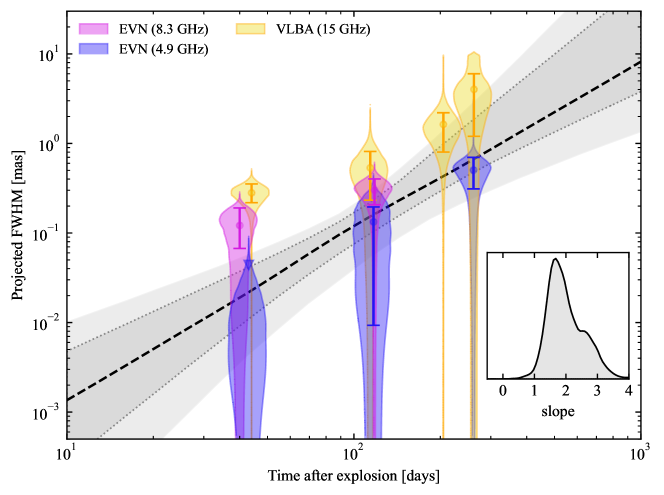
Figure 1: Source size as a function of time. The source size constraints obtained as described in Section 3.1 are shown in the form of violin plots of different colours, centred at the observing time of each epoch and of proportional width to the posterior probability density on the FWHM. In addition, we show the median and 68% credible interval with an error bar of the same color, or the 95% credible upper limit with a triangle if the former interval extends to 0. The black dashed line and the two grey shaded areas show respectively the median, 68% credible interval and 95% credible interval of the posterior predictive distribution of the source size evolution obtained from fitting a power law model $s\propto t_{\mathrm{obs}}^{a}$ to the sizes from all the epochs. The inset shows the posterior probability density on the slope $a$ from such fit.

Figure 1 shows the source size constraints from Table LABEL:tab:log in the form of a ‘violin plot’ whose width is proportional to the posterior probability density on the FWHM, horizontally centred at the time of the observation. Additionally, we show the median and 68% symmetric credible interval on the FWHM by means of an error bar for each observation. In order to quantify the source size evolution from these observations, we fit a simple phenomenological power law evolution model, $s_{\mathrm{m}}(t_{\mathrm{obs}})\propto t_{\mathrm{obs}}^{a}$, to these size measurements, through the method outlined in Sect. 3.2. The resulting posterior probability density on the power law slope is shown in the inset of Figure 1. The median and symmetric 68% credible interval is $a=1.9_{-0.6}^{+0.7}$. We found that 99.966% of the posterior probability (3.6 $\sigma$-equivalent) is located at $a>0$. Therefore, our observations strongly support the expansion of the source. In the main panel of Figure 1, we show with a black dashed line the median of the posterior predictive distribution, that is, the probability distribution of $s_{\mathrm{m}}(t_{\mathrm{obs}})$ at each fixed $t_{\mathrm{obs}}$, as derived from the fit. The dotted lines encompass the 68% symmetric credible interval of the same distribution, filled with a grey shade. A lighter grey shading shows the 95% symmetric credible interval. The steep slope is mainly driven by our EVN 4.9 GHz observation at 43 days post-burst, which provides an upper limit of $0.045\,\mathrm{mas}$, which cannot be explained by simple calibration errors. Conversely, our first 15 GHz VLBA epoch at 44 days is in mild tension with such an evolution, with a measured size $s(44\,\mathrm{d})=0.28_{-0.06}^{+0.08}$ mas. This might be ascribed to coherence loss at the longest baselines, which is more severe at these high frequencies (Martí-Vidal et al., 2010). On the other hand, it could reflect a frequency-dependent source size. To explore that possibility, we repeated the power law size evolution model fit considering only observations at a single frequency. Fig. 2 shows the resulting size evolution for observations at 4.9 GHz (upper panel), 8.3 GHz (middle panel) and 15 GHz (lower panel). The plots are similar to Figure 1, except that the epochs not considered in the fit are shown with a light grey shading. The constraint on $a$ from these fits is somewhat looser, with the medians and symmetric credible intervals being $a=2.1_{-0.8}^{+1.0}$ (4.9 GHz), $a=1.7_{-1.9}^{+2.0}$ (8.3 GHz) and $a=1.1_{-0.3}^{+0.4}$ (15 GHz). While these slopes are formally all compatible with each other, the normalisations of the 4.9 GHz and 15 GHz power laws differ with a $>3\sigma$ significance, as can be evinced from the posterior predictive distributions shown in grey in the panels, suggesting a dependence of the evolution on frequency.

In order to exclude the possibility that our results with the EVN are driven by systematic effects, we carried out a series of tests including the check source J1905$+$1943. We present the results of our tests in Appendix C. The results of these tests indicate that the observed evolution is not driven by systematic errors in the calibrations.

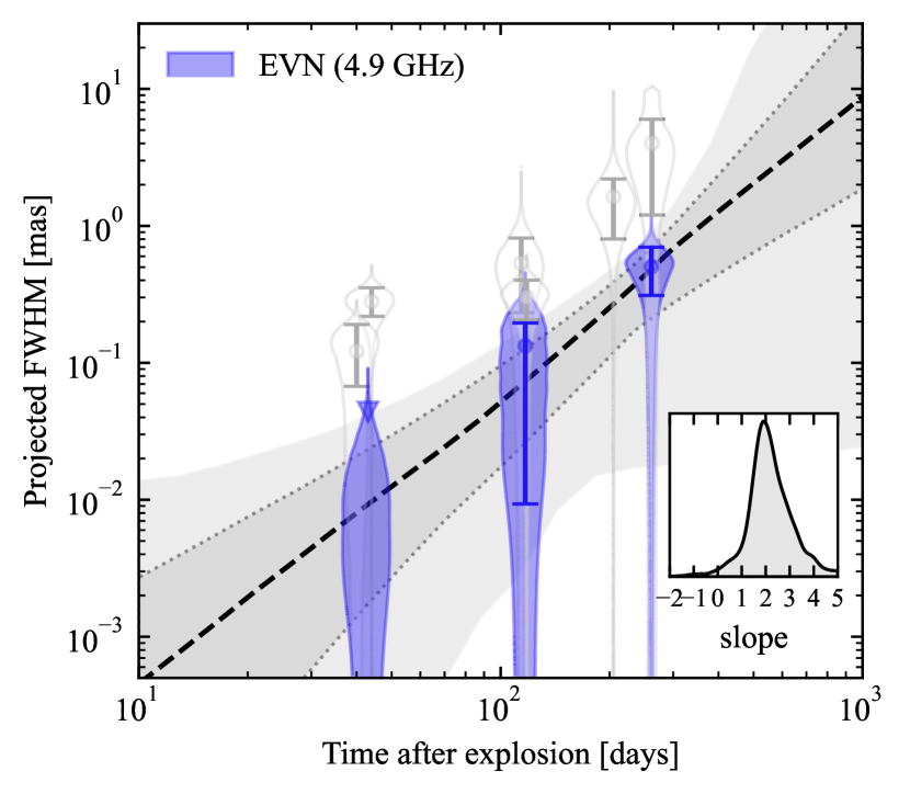
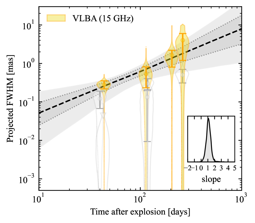
Figure 2: Size evolution considering only observations at a single frequency (upper panel: 4.9 GHz; middle panel: 8.3 GHz; lower panel: 15 GHz). Each panel is similar to Figure 1, except that the epochs not considered in the fit are shown with light grey shading for clarity.

4.2 Apparent proper motion

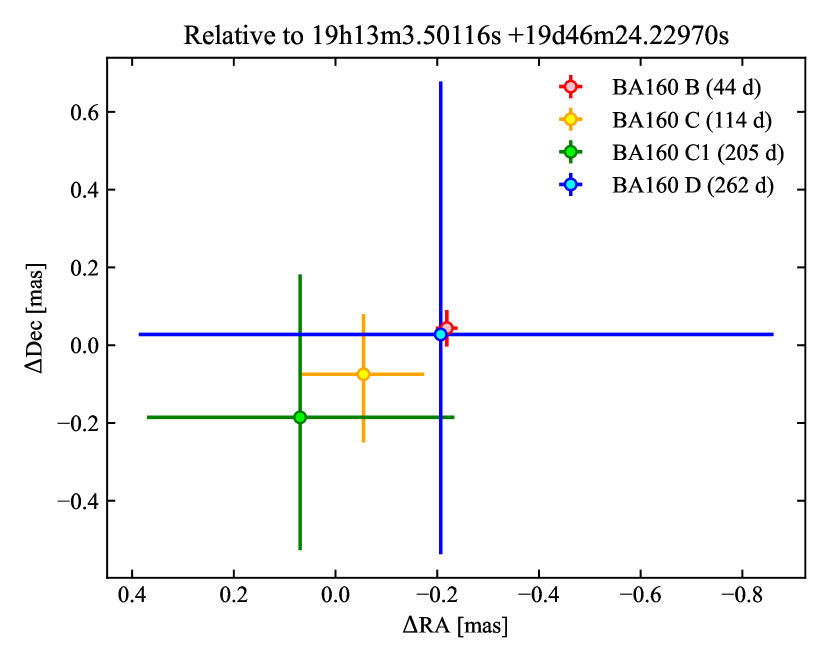
Figure 3: Source position in our VLBA observations. For each epoch, we show an error bar centered on the median position from the circular Gaussian source fit, with bars spanning the symmetric 68% credible interval on the source position in each direction.

VLBI observations can constrain the apparent proper motion of the centroid of the emission and, therefore, the jet viewing angle. The source position at each VLBA epoch is displayed in Fig. 3: our results do not show any significant apparent proper motion between 44 and 262 days post-burst, but our errors can accommodate a displacement of up to about 0.6 mas (at the one-$\sigma$ level) over that period. As shown in Appendix D.2, such an upper limit does not constrain strongly $\theta_{\mathrm{v}}$, which can still be several degrees off the edge of the jet, unless the energy-to-density ratio of the explosion is very large. Still, a number of studies including LHAASO Collaboration et al. (2023) and O’Connor et al. (2023) have used their data to justify a very small $\theta_{\mathrm{v}}$ for GRB 221009A, indicating that we are viewing the jet close to on-axis. The lack of significant proper motion observed during our VLBI campaign is fully consistent with such on-axis scenario.

We note that the EVN campaign is not used for such study because of the change in phase reference source between the second and third epoch. While this change was motivated by the discovery of a closer phase calibrator (and hence a more efficient observing strategy), the different systematics and the lack of a reliable a priori position of the new calibrator prevent a reliable astrometric characterisation.

5 Discussion

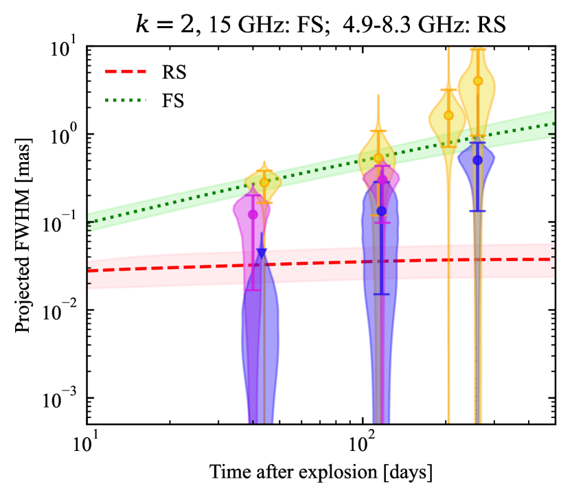
Figure 4: Model size evolution in a FS plus RS scenario. The violins and the error bars show the source size evolution as inferred by our observations, in the same way as in Figure 1. The green dotted line and red dashed lines show the medians of the posterior predictive distributions of the FS and RS size, respectively, as obtained by fitting the physical model described in Appendix D to the sizes shown in the figure, assuming a wind-like external medium, and assuming the FS to dominate at 15 GHz and the RS to dominate at 4.9 and 8.3 GHz. The shaded bands around these lines show the 68% credible interval of the posterior predictive distribution.

The size evolution power law slope $a=1.9_{-0.6}^{+0.7}$ we derived is only marginally compatible (at the 3-$\sigma$ level) with the expected slopes for a Blandford & McKee (1976) blastwave expanding into a homogeneous medium, $\alpha=5/8=0.625$, or a wind-like medium, $\alpha=3/4=0.75$. However, the preferred value for the slope is substantially higher and it even allows for an accelerating ($a>1$) expansion. Moreover, when compared to GRB 030329, the only other burst to date with a measured expansion rate (Taylor et al., 2004), our $a$ value reveals an unprecedented size evolution (Figure 5).

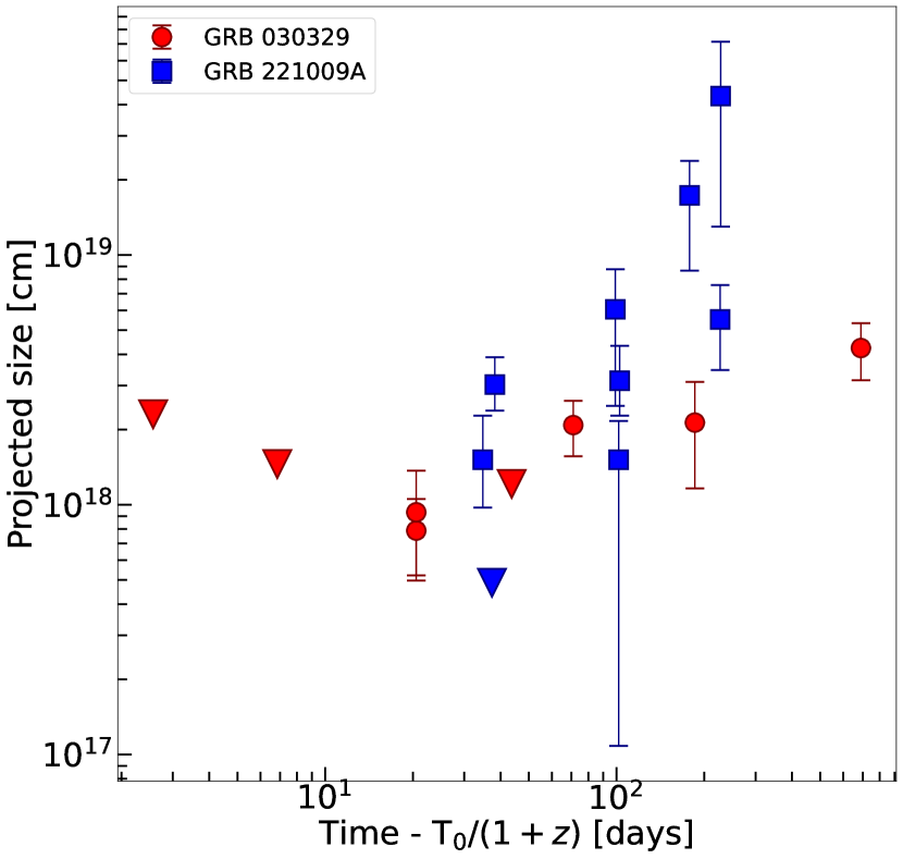
Figure 5: Comparison of size measurements from VLBI observations of GRB 030329 (red circles; Taylor et al. 2004; Pihlström et al. 2007) and GRB 221009A (dark blue squares, this work). Triangles represent upper limits.

It is possible that the apparent rapid expansion favoured by our observations is a result of observing different emission regions at different frequencies.

Many efforts aimed at modelling the multi-wavelength evolution of the GRB 221009A afterglow indicate that the radio wavelengths are likely dominated by a RS component at $t_{\mathrm{obs}}\lesssim 100\,\mathrm{d}$, possibly transitioning to a FS dominated regime at later times. Indeed, the radio afterglow of this GRB cannot be explained by a simple FS propagating either in a wind-like or a homogeneous environment (Ren et al., 2023; Sato et al., 2023; Jia et al., 2023). Using a data set encompassing observations from the GeV to the radio domain, Laskar et al. (2023) showed that the standard afterglow model struggles at explaining the radio emission both with a FS and a RS of a conical jet propagating through a wind-like environment, leading them to invoke an additional component whose temporal evolution does not follow the standard prescriptions. A somewhat improved description could be obtained by including a jet with an angular structure (O’Connor et al., 2023; Gill & Granot, 2023), but it is unclear whether this scenario favors a wind-like or a homogeneous surrounding medium.

Inspired by these results, together with our finding that the size evolution may be frequency-dependent, we explored a scenario where the emission we observed is a superposition of a FS and a RS, leveraging on the model described in Sect. 3.3, with $\@vec{\theta}=(E/A,\theta_{\mathrm{j}},g)$ as our free parameter vector. The external medium power law index was fixed to $k=0$ or $k=2$. Based on the apparent frequency-dependent behaviour, we assumed the higher-frequency observations (15 GHz) to be dominated by the FS, while the lower-frequency ones (4.9 – 8.3 GHz) to be dominated by the RS. For each external density profile, the posterior probability density on $\@vec{\theta}$ was derived through the Bayesian approach described in Sect. 3.2, with a uniform-in-log prior on $E/A$ in the range $[10^{50},10^{60}]$ erg cm³, a uniform prior on $g$ in the range $[(3-k)/2,6]$ and a uniform prior on $\theta_{\mathrm{j}}$ in the range $[0.5,30]$ deg.

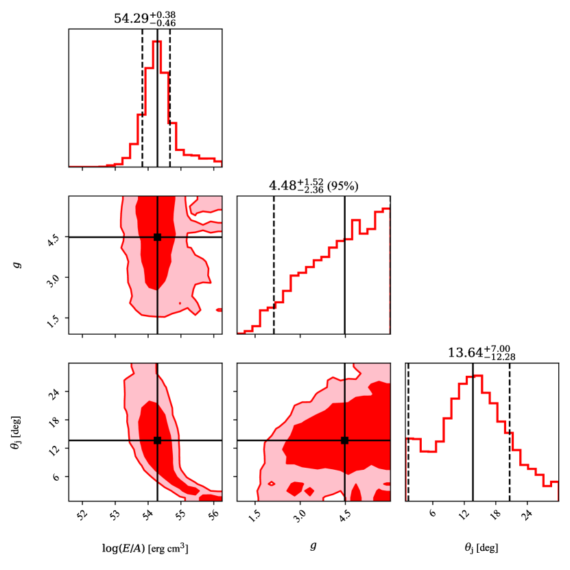
Figure 6: Corner plot of the posterior probability density on the physical model parameters in the wind-like external medium case and assuming the FS to dominate at 15 GHz and the RS to dominate at $4.9$–$8.3$ GHz. The red histograms in the panels on the diagonal show the marginalized posterior probability densities, with black solid vertical lines showing the median and dashed lines showing the 68% credible interval or, if the latter extends to the lower (upper) extremum of the prior range, the 95% upper (lower) limit (values reported on top of the panels). The remaining panels show the smallest contours containing 68% and 95% of the two-dimensional marginalised posterior probabilities on parameter pairs, with the black squares showing the position of the median.

In the homogeneous external medium ($k=0$) case, our model predicts too small a difference between the projected size of the FS and that of the RS, which is insufficient to explain the apparent frequency-dependent size and its evolution. In the case of a wind external medium ($k=2$), on the other hand, the scenario provides a good agreement with the data, as shown in Figure 4. The evolution predicted by the model additionally suggests that the 4.9 GHz observations may transition from being RS-dominated at $t\lesssim 100\,\mathrm{d}$ to being FS-dominated at later times, consistently with the multi-wavelength predictions of O’Connor et al. (2023) and Gill & Granot (2023). The marginalised posterior on $E/A$ shows a clear peak (see Figure 6), with a median and 68% symmetric credible interval $\log(E/A)=54.3_{-0.5}^{+0.4}$ (expressed in erg cm³). Within this scenario, this indicates a high prompt emission efficiency (so that $E<10^{55}\,\mathrm{erg}$) in combination with a relatively high wind density $A>1\,\mathrm{cm^{-3}}$, even though a lower efficiency and wind density can be accommodated if a more stringent prior on the half-opening angle is adopted, as explained below. We also caution here that we have assumed the measured FWHM to correspond to the source diameter as calculated by our model, but this is correct only up to a constant $\xi\sim 1$, which depends on the detailed surface brightness distribution of the source (e.g. Taylor et al., 2004; Pihlström et al., 2007; Salafia et al., 2022). Since $E/A$ is proportional to the fourth power of the FWHM in the $k=2$ case (e.g. Granot et al., 2005), this introduces a possible systematic error of up to a factor of $\xi^{4}\sim 1.4^{4}\approx 4$ on $E/A$ (taking a reference value $\xi=1.4$ as in Pihlström et al. 2007), or equivalently an offset of $0.6$ in $\log(E/A)$. The posterior probability density on $g$ is not very informative, but it indicates that $g>2.1$ (95% credible lower limit), which implies a quite fast deceleration of the RS after it detaches from the FS (hence, in this model, the reverse-shocked material essentially reaches the end of its expansion at around 200 d, as shown in Figure 4). The jet half-opening angle $\theta_{\mathrm{j}}$ is not well constrained ($\theta_{\mathrm{j}}<21\,\mathrm{deg}$ at one $\sigma$), but there is a clear correlation between $E/A$ and $\theta_{\mathrm{j}}$, with larger values of $E/A\gtrsim 10^{55}\,\mathrm{erg}$ being compatible with smaller half-opening angles $\theta_{\mathrm{j}}\lesssim 5$ deg. The inspection of the two-dimensional $(E/A,\theta_{\mathrm{j}})$ posterior (lower left panel of Figure 6) shows that for $\theta_{\mathrm{j}}\lesssim 3$ deg, the preferred $\log(E/A)$ increases up to $55$–$56$.

6 Conclusions

In this manuscript, we presented VLBI observations of the brightest $\upgamma$-ray burst ever observed, GRB 221009A. The high angular resolution provided by the EVN and the VLBA allowed us to constrain the size and the expansion of the blast wave produced by the GRB ejecta for the second time ever. Although still consistent with the standard expansion expected for a Blandford & McKee (1976) blast wave propagating into a circumburst medium (i.e., an ultra-relativistic FS), the derived expansion rate tends to prefer higher values. We suggest that the unusual expansion may be due to our observations transitioning from being dominated by the RS emission to being dominated by the FS emission, in agreement with interpretations that stem from the modelling of the multi-wavelength emission (O’Connor et al., 2023; Gill & Granot, 2023). For our interpretation to hold, the external medium must be wind-like. Our work highlights the crucial role played by multi-wavelength VLBI monitoring of transient events both at early and late times, in order to provide a vital insight into the physics of these sources.

Appendix A EVN observation strategy and data reduction

Table 2: List of antennas that join each observing run.

Code	$t_{\mathrm{obs}}-t_{0}$	Array	Antennas
	[days]
RG013 B	40	EVN	Wb, Ef, Nt, O6, Ur, Tm, Ys, Tr, Hh, Mh
RG013 C	43	EVN	Jb, Wb, Ef, Mc, O8, Ur, Tm, Ys, Tr, Hh
BA160 B	44	VLBA	Fd, Hn, Mk, Nl, Ov, Pt, Sc
BA160 C	114	VLBA	Br, Fd, La, Mk, Nl, Ov, Pt, Sc
RG013 D	117	EVN	Jb, Wb, Ef, Mc, O8, Ur, Tm, Ys, Tr
RG013 E	118	EVN	Wb, Ef, Mc, Nt, O6, Ur, Tm, Ys, Tr, Hh, Mh
BA160 C1	205	VLBA	Br, Fd, Hn, Kp, La, Mk, Nl, Ov, Pt, Sc
RG013 F	261	EVN	Jb, Ef, Mc, Nt, O8, Tm, Ys, Tr, Hh, Ir
BA160 D	262	VLBA	Br, Fd, Hn, Kp, La, Mk, Nl, Ov, Pt, Sc

Wb: Westerbork, 25m; Ef: Effelsberg, 100m; Nt: Noto, 32m; O6: Onsala, 20m; Ur: Urumqi; Tm: Tianma, 65m; Ys: Yebes, 40m; Tr: Torun, 32m; Hh: Hartebeesthoek, 25m; Mh: Metsähovi, 14m; Jb: Jodrell bank (Lovell), 76m; Mc: Medicina, 32m; O8: Onsala, 25m; Ir: Irbene; Br: Brewster, 25m; Fd: Fort Davis, 25m; Hn: Hancock, 25m; Kp: Kitt Peak, 25m; La: Los Alamos, 25m; Mk: Mauna Kea, 25m; Nl: North Liberty, 25m; Ov: Owen Valley, 25m; Pt: Pie Town, 25m; Sc: Saint Croix, 25m.

In this Appendix we provide detailed information on the observation strategy and the data reduction of the EVN observations. As explained in Section 2, the structure of the observations followed a typical phase-referencing experiment. Three compact, extragalactic radio sources J1800$+$3848, J1925$+$2106 and J0121$+$0422 were used as fringe finders and bandpass calibrators throughout the campaign. The target scans, lasting approximately 4.5 and 2.5  minutes at 5 and 8 GHz, respectively, were interleaved with 1.5 minute scans of the phase calibrator. In the first two observations, namely 40 and 43 days post-burst (RG013 B and C), the radio source J905$+$1943 was used as a phase calibrator and the Very Large Array Sky Survey (VLASS) compact radio source J191142$+$1952 was included for testing its suitability as a closer phase reference source ($d=0.33^{\circ}$ from the GRB position). Given the success of such test, J191142$+$1952 was then adopted as phase calibrator in the last three epochs, i.e. from 117 to 261 days post-burst (RG013 D, E and F). In order to inspect the consistency of the calibration procedure, one or multiple compact radio sources were observed approximately every 30 minutes. The phase and amplitude solutions derived from the calibrators were applied to these check sources to verify the quality of the calibration.

The calibration was performed using AIPS (Greisen 2003), following the standard procedure for EVN phase-referenced observations. The amplitude calibration, which accounts for the bandpass response, the antenna gain curves and the system temperatures, was performed using the results from the EVN pipeline. Procedures vlbatecr and vlbampcl were used to correct for the dispersive delay and to calculate the manual single band delay on the fringe finder, respectively. Subsequently, we carried out the global fringe fitting on the phase calibrator with the task fring. Solutions were interpolated and applied to the phase calibrator itself, the check sources and the target with the task clcal. At this point, the calibration procedure differs according to the epoch.

For the first two epochs (RG013 B and C), we carried out the fringe fitting on J1905$+$1943 using a model of the source derived by a concatenation (in CASA, McMullin et al. 2007) and self-calibration (in Difmap) of all the visibilities on the source obtained across the various epochs. This approach is warranted by the stability of the structure of extragalactic sources on the duration of the campaign, and improves the phase, delay, and rate calibration by accounting for the possibile structure of the phase-reference source. We then interpolated the solutions and applied the results to J1905$+$1943 itself, the check source (J1923$+$2010) and GRB 221009A. Lastly, we perform two rounds of self-calibration on J1905$+$1943, first in phase-only, with a solution interval of 2 minutes, and then in amplitude and phase with a solution interval of 60  minutes in AIPS. We interpolated the solutions and applied the results to the phase calibrator itself, the check sources and the target.

In the last three epochs, we employed a different phase calibrator, J191142$+$1952, motivated by the significantly smaller separation from the source (0.33^∘ vs 1.75^∘). If the phase calibrator is closer to the target, any possible decorrelation of the phase solutions is significantly reduced. However, the position of J191142$+$1952 was constrained with a precision of the order of an arcsecond: for VLBI observations, this means that the coordinates of the centre of the source were not aligned with the phase centre of the observation. If one does not correct for the uncertainty in the position, the phase solutions of the global fringe fitting on the phase calibrator will contain a systematic error and the apparent coordinates of the centre of the sources to which these solutions are applied will be incorrect. To avoid this, we started from the fourth epoch, made at 8 GHz, which provides higher angular resolution and therefore a more precise position of the calibrator. We applied the solutions of the first global fringe fitting on J191142$+$1952 to the check sources, J1905$+$1943 and J1923$+$2010, we produced an image of each of them and we compared the apparent coordinates of each source with the actual position, known with an uncertainty of the order of $\sim$mas. Since J1905$+$1943 and J1923$+$2010 appear to be aligned in the sky, with J191142$+$1952 placed in between, we derived the real coordinates with a 1D interpolation at the position of J191142$+$1952 of the offset observed for the check sources. We then re-calculated the visibilities of J191142$+$1952 by fixing the phase centre with the fixvis task in CASA, inserting the new coordinates. We then repeated the entire calibration process iteratively, until the apparent and the real sky coordinates of the check sources were consistent within the resolution of the observation. We corrected the third and fifth epoch using the position derived at 8.3 GHz.

Subsequently, we produced a model of J191142$+$1952 in Difmap and we used the model as input to perform the global fringe fitting of the phase calibrator in AIPS, in order to take into account any possible structure of J191142$+$1952 and correct for it. We interpolated the solutions and we applied them to J191142$+$1952, J1905$+$1943, J1923$+$2010 and GRB 221009A. Lastly, we performed a round of amplitude and phase self-calibration of J191142$+$1952 in AIPS, using a solution interval of 2 minutes and we applied the interpolated solutions to J191142$+$1952, J1905$+$1943, J1923$+$2010 and GRB 221009A. After each of the aforementioned steps of the procedure, the derived solutions were inspected and bad data were properly flagged.

Images of the target and the check sources were produced using Difmap. Unfortunately, due to the sparse $(u,v)$ plane coverage and the distance from the phase calibrator, J1923$+$2010 was not usable to check the consistency of the calibration process.

Appendix B Circular Gaussian fits to source visibilities

In this appendix we provide more detailed information about our circular Gaussian fits to source visibilities from our VLBI observations. We assumed a chi-squared log-likelihood for the visibilities, namely

$$\begin{array}[]{l}\ln\mathcal{L}\left(\{\mathcal{V}_{i}\}_{i=1}^{N}\,|\,\@vec{x}\right)=-\frac{1}{2}\sum_{i=0}^{N}w_{i}\left\{\left[\mathcal{V}_{R,\mathrm{m}}(u_{i},v_{i},\@vec{x})-\mathcal{V}_{R,i}\right]^{2}\right.+\\ +\left.\left[\mathcal{V}_{I,\mathrm{m}}(u_{i},v_{i},\@vec{x})-\mathcal{V}_{I,i}\right]^{2}\right\}\end{array}$$ (3)

where $\mathcal{V}_{R,i}$ and $\mathcal{V}_{I,i}$ are the real and imaginary part, respectively, of the $i$-th visibility measurement $\mathcal{V}_{i}$, corresponding to position $(u_{i},v_{i})$ on the $(u,v)$ plane, and $w_{i}$ is its data weight as determined by our calibration procedure. By definition $w_{i}=\sigma_{i}^{-2}$, where $\sigma_{i}$ is the uncertainty in the visibility measurement. Our source model is represented by $\mathcal{V}_{R,\mathrm{m}}(u,v,\@vec{x})$ and $\mathcal{V}_{I,\mathrm{m}}(u,v,\@vec{x})$, which are the real and imaginary parts of a circular Gaussian source model defined by

$$\mathcal{V}_{\mathrm{m}}(\@vec{x})=F_{\nu}e^{-2\pi^{2}\left(\frac{s}{\sqrt{8\ln 2}}\right)^{2}\left(u^{2}+v^{2}\right)-2\pi j(u\rho+v\delta)},$$ (4)

where $j=\sqrt{-1}$, $F_{\nu}$ is the total flux density, $s$ the full width at half maximum (FWHM), and $\rho$ and $\delta$ the spherical offsets of the source with respect to the phase centre. These parameters collectively constitute the components of the parameter vector $\@vec{x}=(F_{\nu},s,\rho,\delta)$. By Bayes’ theorem, we defined the posterior probability on $\@vec{x}$, given our data $\{\mathcal{V}_{i}\}_{i=1}^{N}$, as

$$P\left(\@vec{x}\,|\,\{\mathcal{V}_{i}\}_{i=1}^{N}\right)\propto\pi(\@vec{x})\mathcal{L}\left(\{\mathcal{V}_{i}\}_{i=1}^{N}\,|\,\@vec{x}\right),$$ (5)

where $\pi(\@vec{x})$ is the prior probability on the parameters. For the latter, we adopted simple independent uniform priors on each parameter, with the due bounds $F_{\nu}>0$ and $s>0$. Where necessary, in order to prevent the fitting procedure from picking up some noise peak instead of the actual source, we restricted the position $(\rho,\delta)$ to within a small angular distance $\Delta_{\mathrm{pos}}\sim 1\,\mathrm{mas}$ from the peak $(\rho_{0},\delta_{0})$ of the dirty map constructed with AIPS. Therefore, our prior took the form

$$\begin{split}&\pi(\@vec{x})\propto\Theta(F_{\nu})\Theta(s)\Theta(\rho-\rho_{0}+\Delta_{\mathrm{pos}})\Theta(\rho_{0}+\Delta_{\mathrm{pos}}-\rho)\times\\ &\times\Theta(\delta-\delta_{0}+\Delta_{\mathrm{pos}})\Theta(\delta_{0}+\Delta_{\mathrm{pos}}-\delta),\end{split}$$ (6)

where $\Theta$ is the Heaviside step function. Only for the VLBA D epoch, we added the constraint $s<10\,\mathrm{mas}$ (i.e. we added a factor $\Theta(10\,\mathrm{mas}-s)$ to the prior) to remove a secondary peak of the posterior at $s\sim 30\,\mathrm{mas}$, which we consider as spurious. For each epoch, we sampled the posterior probability using the emcee (Foreman-Mackey et al. 2013) python package. We initialised emcee with the initial guess $\@vec{x}=(I_{\nu,\mathrm{pk}},10^{-4}\,\mathrm{mas},\rho_{0},\delta_{0})$, where $I_{\nu,\mathrm{pk}}$ is the peak surface brightness (expressed in Jy/beam) in the dirty map, corresponding to an unresolved circular Gaussian source at the position of the peak of the dirty map and with a flux density that yields the observed peak surface brightness. We then ran $3000$ iterations of the MCMC with 32 walkers, for a total of $96000$ samples of the posterior probability density for each epoch. The results were constructed after discarding the initial 30% of these samples as burn-in.

Figure 7 shows corner plots that visualize the properties of the posterior probability density on $(F_{\nu},\mathrm{FWHM})$ for our EVN 4.9 GHz epochs. Figures 8 and 9 show the corresponding corner plots for our EVN 8.3 GHz epochs and for our VLBA 15 GHz epochs, respectively.

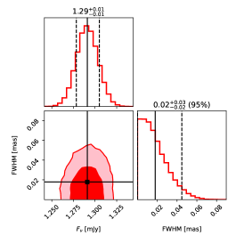
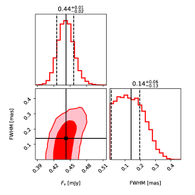
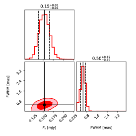
Figure 7: Posterior probability distribution on the source size and flux density in our EVN 4.9 GHz epochs at $T-T_{0}=43$ (RG1013 C, left), 117 (RG013 D, center) and 261 (RG013 F, right) days. In each corner plot, the top-left and bottom-right sub-panels show histograms of the posterior samples of $F_{\nu}$ and FWHM, with the vertical solid lines showing the median and the vertical dashed lines bracketing the 68% credible interval or, if the latter extends to 0, the 95% credible upper limit. The bottom-left sub-panel of each corner plot shows the smallest contours containing 68% and 95% of the posterior probability.

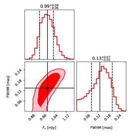
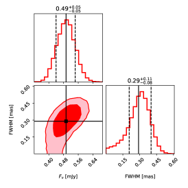
Figure 8: Similar to Figure 7, but for our EVN 8.3 GHz epochs at $T-T_{0}=40$ (EVN B, left) and 118 (EVN E, right) days.

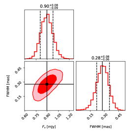
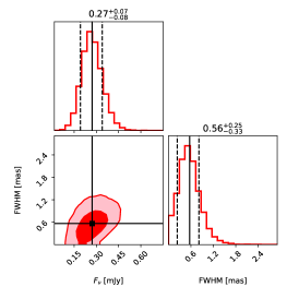
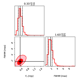
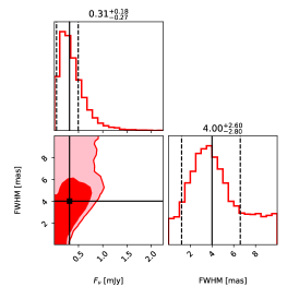
Figure 9: Similar to Figure 7, but for our VLBA 15 GHz epochs at $T-T_{0}=44$ (VLBA B, upper left), 114 (VLBA C, upper right), 205 (VLBA C1, lower left) and 262 (VLBA D, lower right) days.

Appendix C Tests on the evolution of the flux density and the size

In this Appendix we present tests on the EVN observational results that we carried out in order to exclude the possibility that the measured evolution of the GRB size is a result of systematic effects. These tests include the check source J1905$+$1943. Unfortunately, due to the sparse $(u,v)$ plane coverage and the large separation, J1923$+$2010 could not be used to get meaningful constraints. First, the measured GRB afterglow size as a function of the equivalent radius (left panel) and area (right panel) of the synthesised beam are presented in Fig. 10. These quantities are clearly not correlated, hence we can exclude the possibility that the observed expansion of the GRB is driven by a systematic change in the width of the synthesised beam. In Fig. 11, the flux density (left panel) and the size (right panel) of GRB 221009A and the check source J1905$+$1943 are compared. The decrease in the GRB 221009A flux density is not accompanied by a variation of the J1905$+$1943 flux density, as expected. In the 8.3 GHz observations, the size of J1905$+$1943 is constant, as expected, while that of the GRB afterglow shows a mild evidence for an increase across the two observations. At 4.9 GHz, the size we measure for J1905$+$1943 differs by approximately a factor of 2 between the first two epochs (C and D, where it is approximately 188 $\upmu$as) and the last epoch (F, where it is 402 $\upmu$as). On the other hand, across the same observations, the FWHM of the GRB afterglow varies by almost an order of magnitude. Therefore, the variation in the observed size of the GRB afterglow cannot be ascribed to a systematic effect due to an imprecise calibration. Concerning the VLBA, no test was performed because of the lack of close enough check sources.

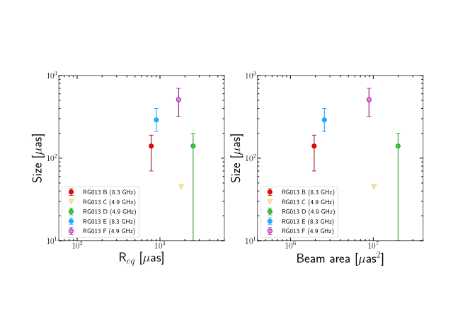
Figure 10: Estimates of the FWHM of the GRB as a function of the equivalent radius (left panel) and the total area (right panel) of the synthesised beam for the EVN observations.

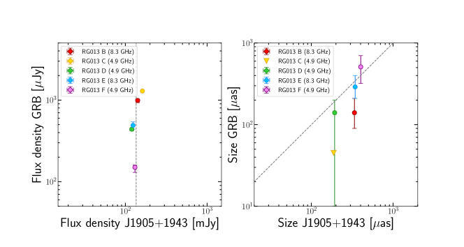
Figure 11: Flux density (left panel) and size (right panel) of GRB 221009A and J1905$+$1943 in the EVN observations. The average flux density of J1905$+$1943 (left panel) and the 1:1 correlation (right panel) are shown as grey dashed lines for the sake of comparison.

Appendix D Model of the projected size and proper motion of the forward and reverse shock

D.1 Dynamics and size evolution

In the following, we describe an approximate analytical model of the dynamics of the forward and reverse shocks, based on similar calculations as Kobayashi et al. (1999); Kobayashi & Zhang (2003); Yi et al. (2013). The aim is to extend approaches such as those described in Oren et al. (2004) and Granot et al. (2005) by including the reverse shock, which was not considered there. We assume a cold external medium with a power law density profile $\rho=Am_{\mathrm{p}}(R/R_{\star})^{-k}$, where $R$ is the radial distance from the progenitor, $m_{\mathrm{p}}$ is the proton mass and $A$ is the number density at a reference radius $R_{\star}=5.5\times 10^{17}\,\mathrm{cm}$. With this definition, $A$ plays the role of either the homogeneous interstellar medium (ISM) number density, $A\equiv n$ if $k=0$, or that of the wind density parameter, $A\equiv A^{\star}$ if $k=2$. We assume a simplified description of the jet as a cold, kinetic-energy-dominated shell with uniform initial bulk Lorentz factor $\Gamma_{0}\approx 316\,\Gamma_{0,2.5}\gg 1$ and constant isotropic-equivalent kinetic luminosity $L=E/T$, where $E=10^{55}\,E_{55}\,\mathrm{erg}$ is the isotropic-equivalent jet energy and $T\sim T_{90}/(1+z)\approx 500\,T_{2.7}\,\mathrm{s}$ is the lifetime of the central engine. The Sedov length associated with this shell is $\ell_{\mathrm{S}}=[(3-k)E/(4\pi AR_{\star}^{k}m_{\mathrm{p}}c^{2})]^{1/(3-k)}$. As this shell expands into the external medium at relativistic speed, a forward shock (FS) arises, which sweeps the external medium moving with a Lorentz factor $\Gamma_{\mathrm{FS,0}}\sim\sqrt{2}\Gamma_{0}$. The shocked external medium resides in the region contained between the FS and the contact discontinuity (CD) that separates it from the jet material. Since this implies some deceleration of the jet material behind the CD as well, as soon as the ram pressure of such material overcomes the pressure in the jet (formally already at R=0 given our assumption of a cold jet), a reverse shock (RS) also arises, which separates shocked from cold un-perturbed jet material. Let us indicate with numbers from 1 to 4 the un-perturbed external medium, shocked external medium, shocked jet and un-perturbed jet respectively, as usual. The RS is initially non-relativistic (i.e. the relative speed of regions 3 and 4 is $\beta_{\mathrm{34}}\ll 1$), but it can become relativistic before the RS crosses the whole jet if the condition (Sari & Piran 1995; Kobayashi et al. 1999; Chevalier & Li 2000; Kobayashi & Zhang 2003; Zou et al. 2005; Yi et al. 2013)

$$\frac{E}{A}<\frac{4\pi m_{\mathrm{p}}c^{2}R_{\star}^{k}}{3-k}\left(cT\right)^{3-k}\Gamma_{0}^{2(4-k)}\approx\left\{\begin{array}[]{cr}2.1\times 10^{57}\Gamma_{0,2.5}^{8}T_{2.7}^{3}\,\mathrm{erg\,cm^{3}}&k=0\\ 8.6\times 10^{56}\Gamma_{0,2.5}^{3}T_{2.7}\,\mathrm{erg\,cm^{3}}&k=2\\ \end{array}\right.$$ (7)

is satisfied, in which case the jet deceleration is said to be in the ‘thick shell regime’. In the following we describe the dynamics in such regime, and we defer to later the treatment of the opposite, ‘thin shell’ regime. For the homogeneous ISM case, $k=0$, the RS transitions from Newtonian to relativistic at a radius $R_{\mathrm{N}}\sim\ell_{\mathrm{S}}^{3/2}[(12cT)^{1/2}\Gamma_{0}^{2}]^{-1}\sim 3\times 10^{16}\,E_{55}^{1/2}A_{0}^{-1/2}\Gamma_{0,2.5}^{-2}T_{2.7}^{-1/2}\,\mathrm{cm}$, while in the wind case, $k=2$, the RS is always relativistic as long as condition 7 holds. As regions 2 and 3 decelerate due to the increasing amount of swept external medium mass, at some point the RS crosses the whole jet, at a radius

$$R_{\otimes}=(4(3-k)cT)^{1/(4-k)}\ell_{\mathrm{S}}^{(3-k)/(4-k)}.$$ (8)

Before $R_{\otimes}$, regions 2 and 3 effectively expand at the same Lorentz factor $\Gamma$, whose evolution can be described approximately as

$$\Gamma(R)\sim\left\{\begin{array}[]{lr}\Gamma_{0}&R\leq R_{\mathrm{N}}\\ \frac{\ell_{\mathrm{S}}^{(3-k)/4}}{\left[4(3-k)cT\right]^{1/4}}R^{-(2-k)/4}&R_{\mathrm{N}}<R\leq R_{\otimes}\end{array}\right..$$ (9)

The Lorentz factor of region 3 at the end of the RS crossing is therefore $\Gamma_{\otimes}=\left[\ell_{\mathrm{S}}/\left(4(3-k)cT\right)\right]^{(3-k)/[2(4-k)]}$. At radii larger than $R_{\otimes}$, the Lorentz factor of region 2 follows the Blandford & McKee (1976) relativistic blastwave evolution, $\Gamma_{2}\sim(R/\ell_{\mathrm{S}})^{-(3-k)/2}$. This holds as long as the lateral expansion of the shocked material in region 2 is negligible: numerical simulations and analytical arguments (Kumar & Granot 2003; van Eerten et al. 2010; De Colle et al. 2012; Lyutikov 2012; Granot & Piran 2012, e.g.) show that such expansion has a very limited impact on the dynamics until region 2 becomes mildly relativistic, which justifies such assumption. In the homogeneous ISM case, $k=0$, the subsequent evolution of $\Gamma_{3}$ has been historically described phenomenologically (Kobayashi & Sari 2000) as $\Gamma_{3}=\Gamma_{\otimes}(R/R_{\otimes})^{-g}$, with $g$ being typically fixed at around $g\sim 2$ in the case of a non-relativistic RS, or at $g=1.5$ (i.e. the same evolution as the FS) in the case of a relativistic RS (when condition 7 holds), based on insights from the numerical simulations described in Kobayashi et al. (1999) and Kobayashi & Sari (2000). Physically, the different evolution is likely related to the conversion of internal to kinetic energy in region 3 as it expands, which allows it to remain ‘attached’ to region 2 as long as its temperature is relativistic. For historical reasons, in the case of a wind environment, $k=2$, the evolution in this phase has been always assumed to track that of the FS (i.e. $g=0.5$), despite the lack of numerical simulations to compare to. We argue here that generally, as the internal energy conversion terminates, region 3 must eventually ‘detach’ and expand backwards (as seen from the CD) into a rarefaction wave, and thus the evolution of $\Gamma_{3}$ with radius must steepen. In order to estimate the radius $R_{\mathrm{det}}$ at which regions 2 and 3 detach, we need to know the evolution of the internal energy in region 3, $E_{\mathrm{int,3}}$ (as measured in the comoving frame of region 3). From the first equation of thermodynamics, $d\ln E_{\mathrm{int,3}}=(1-\hat{\gamma})d\ln V_{3}^{\prime}$, where $\hat{\gamma}$ is the adiabatic index and $V_{3}^{\prime}$ is the comoving volume of region 3. We assume $V_{3}^{\prime}\propto R^{3}/\Gamma_{3}$. Right after the shock crossing regions 2 and 3 still move together, hence we can assume $\Gamma_{3}\propto R^{-(3-k)/2}$, which leads to $E_{\mathrm{int,3}}=E_{\mathrm{int,3,\otimes}}\left(R/R_{\otimes}\right)^{(1-\hat{\gamma})(9-k)/2}$. Taking the internal energy at the end of RS crossing to be $E_{\mathrm{int,3,\otimes}}\sim(\Gamma_{34,\otimes}-1)m_{3}c^{2}\sim(\Gamma_{\otimes}/\Gamma_{0}+\Gamma_{0}/\Gamma_{\otimes})m_{3}c^{2}/2$ (where $\Gamma_{34,\otimes}$ is the relative Lorentz factor of regions 3 and 4 at the RS crossing radius, and $m_{3}$ is the jet rest mass), we finally conclude that the effective dimensionless temperature in region 3 evolves as

$$\Theta_{3}\equiv E_{\mathrm{int,3}}/m_{3}c^{2}\sim\left[\frac{1}{2}\left(\frac{\Gamma_{\otimes}}{\Gamma_{0}}+\frac{\Gamma_{0}}{\Gamma_{\otimes}}\right)-1\right]\left(R/R_{\otimes}\right)^{(1-\hat{\gamma})(9-k)/2}.$$ (10)

Assuming $\hat{\gamma}=4/3$ since the RS is relativistic, we finally obtain the detachment radius from the condition $\Theta_{3}(R_{\mathrm{det}})=1$, which yields

$$R_{\mathrm{det}}=\mathrm{max}\left\{\left[\frac{1}{2}\left(\frac{\Gamma_{\otimes}}{\Gamma_{0}}+\frac{\Gamma_{0}}{\Gamma_{\otimes}}\right)-1\right]^{6/(9-k)},1\right\}R_{\otimes},$$ (11)

where the maximum function is introduced to account for cases where $\Theta_{3}<1$ at $R_{\otimes}$, in which case $R_{\mathrm{det}}=R_{\otimes}$.

Based on these considerations, we model the evolution of $\Gamma_{3}$ after RS crossing as

$$\Gamma_{3}(R)=\left\{\begin{array}[]{lr}\Gamma_{\otimes}\left(\frac{R}{R_{\otimes}}\right)^{-(3-k)/2}&R_{\otimes}\leq R<R_{\mathrm{det}}\\ \Gamma_{\otimes}\left(\frac{R_{\mathrm{det}}}{R_{\otimes}}\right)^{-(3-k)/2}\left(\frac{R}{R_{\mathrm{det}}}\right)^{-g}&R_{\mathrm{det}}\leq R\\ \end{array}\right..$$ (12)

The above relations completely specify the evolution of $\Gamma_{2}$ and $\Gamma_{3}$ with radius as a function of the Sedov length $\ell_{\mathrm{S}}$, initial Lorentz factor $\Gamma_{0}$ and jet duration $T$ for a given choice of $k$ and $g$ in the thick shell regime. The thin shell regime is obtained (Kobayashi et al. 1999) by setting all transition radii equal to the ‘deceleration’ radius, $R_{\mathrm{N}}=R_{\otimes}=R_{\mathrm{det}}=\ell_{\mathrm{S}}/\Gamma_{0}^{2/(3-k)}$. The relation between the radius $R$ and the observer time for region $i\in\{2,3\}$ can be obtained by noting that most of the emission that the observer receives comes from material moving at an angle $\sim\Gamma_{i}^{-1}$ from the line of sight, for which the arrival time is $t_{\mathrm{obs}}/(1+z)=t(R)-R\beta_{i}(R)/c$, where $\beta_{i}=\sqrt{1-\Gamma_{i}^{-2}}$. The progenitor-frame time $t$ as a function of the radius can be obtained by integrating $t(R)=\int_{0}^{R}\mathrm{dR}/(\beta_{i}c)$. By numerically inverting the resulting relation between $t_{\mathrm{obs}}$ and $R$, we finally obtain $R_{i}(t_{\mathrm{obs}})$, and thus $\Gamma_{2}(t_{\mathrm{obs}})$ and $\Gamma_{3}(t_{\mathrm{obs}})$. The projected angular diameter of region $i=2,3$ is then approximately (e.g. Oren et al. 2004)

$$s_{\mathrm{m},i}(t_{\mathrm{obs}})\sim 2\frac{R_{i}(t_{\mathrm{obs}})}{d_{\mathrm{A}}}\times\left\{\begin{array}[]{lr}\Gamma_{i}^{-1}(t_{\mathrm{obs}})&\Gamma_{i}(t_{\mathrm{obs}})\geq 1/\theta_{\mathrm{j}}\\ \theta_{\mathrm{j}}&\Gamma_{i}(t_{\mathrm{obs}})<1/\theta_{\mathrm{j}}\\ \end{array}\right.,$$ (13)

where $\theta_{\mathrm{j}}$ is the jet half-opening angle. We find that the predicted size of the FS from this model matches that of the more refined model of Granot et al. (2005) within 10% for $k\in\{0,2\}$ in the self-similar deceleration stage.

D.2 Proper motion

If the jet is observed at a viewing angle $\theta_{\mathrm{v}}>\theta_{\mathrm{j}}$, an apparent displacement of the projected image is expected. As long as $\Gamma^{-1}<(\theta_{\mathrm{v}}-\theta_{\mathrm{j}})$, the observed emission is dominated by the border of the shock closest to the observer. Its apparent displacement $\Delta$ can be modelled effectively as that of a point source moving at $\sim c$ at an angle $\theta_{\mathrm{v}}-\theta_{\mathrm{j}}$ away from the line of sight, so that the displacement increases linearly in time, $\Delta\propto t_{\mathrm{obs}}$. For $(\theta_{\mathrm{v}}-\theta_{\mathrm{j}})<\Gamma^{-1}<(\theta_{\mathrm{v}}+\theta_{\mathrm{j}})$, the emission is dominated by material moving at $\sim 1/\Gamma$ from the line of sight, hence the displacement evolves as $\Delta(t_{\mathrm{obs}})\sim R(t_{\mathrm{obs}})/\Gamma(t_{\mathrm{obs}})d_{\mathrm{A}}$, with $R(t_{\mathrm{obs}})$ being the same as in the on-axis case. Eventually, for $\Gamma^{-1}>(\theta_{\mathrm{v}}+\theta_{\mathrm{j}})$, the emission is dominated by the material at the shock border farthest from the observer, and the displacement is therefore $\Delta(t_{\mathrm{obs}})\sim R(t_{\mathrm{obs}})\sin(\theta_{\mathrm{v}}+\theta_{\mathrm{j}})/d_{\mathrm{A}}$. The transition times $t_{\mathrm{j,obs,\pm}}$ that separate the three regimes described above can be obtained by setting $\Gamma(t_{\mathrm{obs}})=(\theta_{\mathrm{v}}\pm\theta_{\mathrm{j}})^{-1}$ in the on-axis case, which we do numerically.

The model described here neglects the effects of lateral expansion of the shock and of a non-trivial jet structure outside the ‘core’ of half-opening angle $\theta_{\mathrm{j}}$. The former would generally slow down the evolution, so that the displacement predicted by this model can be considered as an upper limit. The latter would change (generally steepen) the slope of the evolution before the time $t_{\mathrm{j,obs,-}}$ at which the jet core starts coming into sight, but not thereafter. For the most likely parameters, our observations are at $t_{\mathrm{obs}}>t_{\mathrm{j,obs,-}}$, so that the effects of a jet structure are unimportant for this particular source.

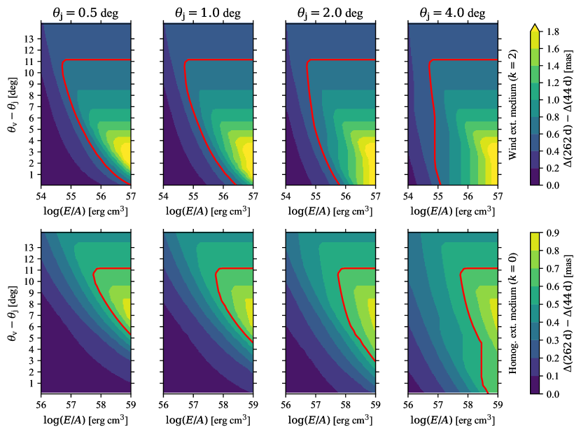
Figure 12: Constraint on the viewing angle from the absence of an observed source apparent displacement in our VLBA observations. In each panel, filled contours show the source centroid displacement expected between 44 d and 262 d, color coded as shown in the colorbar on the right, as a function of the $E/A$ ratio and of the off-edge viewing angle $\theta_{\mathrm{v}}-\theta_{\mathrm{j}}$. The red contour shows $\Delta(262\,\mathrm{d})-\Delta(44\,\mathrm{d})=0.6\,\mathrm{mas}$, which represents the largest displacement compatible at 1 $\sigma$ with our observations. The red contour hence contains the excluded parameter region. The upper panel row refers to a wind-like external medium, while the lower row refers to a homogeneous external medium. Each column assumes a different jet half-opening angle, as reported on top of the column.

Figure 12 shows the displacement predicted by such a model between 44 d and 262 d, assuming the emission to be dominated by the FS (which produces the largest displacement, and dominates the VLBA data according to our interpretation) for different assumptions on $\theta_{\mathrm{j}}$ (varying across columns) and on the external medium power law index (top row: $k=2$; bottom row: $k=0$), as a function of the off-edge viewing angle $\theta_{\mathrm{v}}-\theta_{\mathrm{j}}$ and of the energy to density ratio $E/A$. These predictions show that our upper limit on the observed displacement only excludes off-edge viewing angles between a few degrees and around 11 degrees, combined with large energy to density ratios $E/A\gtrsim 10^{55}\,\mathrm{erg\,cm^{3}}$ for $k=2$, or rather extreme $E/A\gtrsim 10^{58}\,\mathrm{erg\,cm^{3}}$ for $k=0$. Viewing angles larger than $\theta_{\mathrm{v}}-\theta_{\mathrm{j}}\sim 11\,\mathrm{deg}$ cannot be constrained because in that case the shock is in the ‘point-source at the jet edge’ regime all the way to $262$ d, with a rather small apparent transverse velocity. On the other hand, such a large viewing angle would be very unlikely given the huge $\upgamma$-ray isotropic-equivalent energy of this source.