Implicit and explicit matching of non-proper transfer functions in the Loewner framework

Abstract

The reduced-order modeling of a system from data (also known as system identification) is a classical task in system and control theory and well understood for standard linear systems with the so-called Loewner framework as one of many established approaches. In the case of descriptor systems for which the transfer function is not proper anymore, recent research efforts have addressed strategies to deal with the non-proper parts more or less explicitly. In this work, we propose a variant of a Loewner matrix-based interpolation algorithm that implicitly addresses possibly non-proper components of the system response. We evaluate the performance of the suggested approach by comparing against recently-developed explicit algorithms for which we propose a linearized Navier-Stokes model with a significant non-proper behavior as a benchmark example.

An extension of the Antoulas-Anderson algorithm to implicitly identify non-proper parts of the transfer function and a flow simulation benchmark example with a significant linear term.

1 Introduction

Accurate modeling of physical phenomena often leads to large-scale dynamical systems that require long simulation times and storage of large amount of data. In this context, model order reduction (MOR) aims at obtaining much smaller and simpler models that are still capable of accurately representing the behavior of the original process. The Loewner framework (LF) [1] is very appealing due to its data-driven nature, which makes it non-intrusive as it does not use the full or exact description of the model. Hence, it can be viewed as a data-driven reduced-order modeling tool (in this context, data are frequency response measurements).

Dynamical systems characterized by differential algebraic equations (DAEs) (referred to as descriptor, singular or semi-state systems) are not only of theoretical interest but also have a broad application range. In chemistry, for example, the additional algebraic equations account for thermodynamic equilibrium relations, steady state assumptions, or empirical correlations [2]. In mechanics, DAEs result from holonomic and non-holonomic constraints [3]. We refer the reader to [4] for an in-depth account of analysis and numerical solution of DAEs, and to contributions from the last two decades that extended classical MOR methods to specific cases of dynamical systems with DAEs in [5, 3, 6, 7].

The LF is based on the Loewner pencil that allows solving the generalized realization problem for linear time-invariant (LTI) systems [8], and obtaining reduced-order models through compression based on the Singular Value Decomposition (SVD). The Loewner matrix method of Antoulas-Anderson (AA) in [9] also uses a Loewner matrix to construct interpolatory rational functions, but it is based on barycentric representations of such functions, as opposed to the Loewner pencil formulation in LF. To broaden the applicability of LF, extensions of the LF have recently been proposed for specific classes of dynamical systems characterized by DAEs, such as the approaches in [10, 11].

In this class, the linearized Navier-Stokes equations (NSEs) are a meaningful test case. The standard velocity-pressure formulation of the NSEs comes with a matrix-pencil of index 2; however, the linear term in the transfer function only occurs if the control happens to affect the continuity equation; cp. [12]. In a theoretical model, this scenario hardly ever occurs from first principles. Nonetheless, in the numerical realization of Dirichlet conditions, such a control term may appear; cp. [13]. In this work, we present a discretization approach that explicitly treats the Dirichlet control such that the linear part in the transfer function becomes a significant part of the model. We test established and recent developments of the LF on this model in terms of the qualitative identification of the non-proper terms and the quantitative approximation of the overall transfer function.

As the title suggests, the explicit approach for matching of non-proper transfer functions in the LF will be made according to [11]. There, the polynomial coefficients are explicitly estimated and then, the data are post-processed so that a proper rational function can be fitted instead. Then, the implicit approach consists of an adaptation of the AA method in [9] to account for such polynomial terms, directly in the barycentric form of the fitted rational function. The latter has the advantage that no estimation of polynomial coefficient or post-processing is required.

2 The tangential rational interpolation problem

For MIMO (multi-input multi-output) systems, the samples of the transfer function ${\mathbf{H}}(s)={\mathbf{C}}(s{\mathbf{E}}-{\mathbf{A}})^{-1}{\mathbf{B}}+{\mathbf{D}}$ are $p\times m$ matrices. So, in the case of rational matrix interpolation, one possibility is to interpolate along specific directions otherwise, the dimension will scale with the lengths of the input-output spaces. To avoid this, a viable way is to address the so-called tangential interpolation problem (see, e.g., [1, 14]).

We are given a set of input/output response measurements characterized by left interpolation points $\{\mu_{i}\}_{i=1}^{q}\subset{\mathbb{C}}$, using left tangential directions $\{\boldsymbol{\ell}_{i}\}_{i=1}^{q}\subset{\mathbb{C}}^{p}$, and producing left responses $\{{\mathbf{v}}_{i}\}_{i=1}^{q}\subset{\mathbb{C}}^{m}$, together with right interpolation points $\{\lambda_{i}\}_{i=1}^{k}\subset{\mathbb{C}}$, using right tangential directions: $\{{\mathbf{r}}_{i}\}_{i=1}^{k}\subset{\mathbb{C}}^{m}$, producing right responses: $\{{\mathbf{w}}_{i}\}_{i=1}^{k}$.

We are thus given the left data subset $(\mu_{j};{\boldsymbol{\ell}_{j}}^{T},{\mathbf{v}}_{j}^{T})$, $j=1,\ldots,q$, and also the right data subset $(\lambda_{i};{\mathbf{r}}_{i},{\mathbf{w}}_{i})$, $i=1,\ldots,k$. The goal is to find a rational $p\times m$ matrix function ${\mathbf{H}}(s)$, such that the tangential interpolation conditions below are matched:

$$\begin{split}{\mathbf{H}}(\lambda_{i}){\mathbf{r}}_{i}&={\mathbf{w}}_{i},~{}i=1,\ldots,k,\\ \boldsymbol{\ell}_{j}^{T}{\mathbf{H}}(\mu_{j})&={\mathbf{v}}_{j}^{T},~{}j=1,\ldots,q.\end{split}$$ (1)

The left data subset is interpolation points rearranged as:

$${\mathbf{M}}=\text{diag}(\mu_{1},\ldots,\mu_{q})\in{\mathbb{C}}^{q\times q},\begin{array}[]{l}{\mathbf{L}}^{T}=[\boldsymbol{\ell}_{1}~{}~{}\cdots~{}~{}\boldsymbol{\ell}_{q}]\in{\mathbb{C}}^{p\times q},\\[5.69054pt] {\mathbb{V}}^{T}=[{\mathbf{v}}_{1}~{}~{}\cdots~{}~{}{\mathbf{v}}_{1}]\in{\mathbb{C}}^{m\times q}.\end{array}$$ (2)

while the right data subset is arranged as:

$$\boldsymbol{\Lambda}=\text{diag}(\lambda_{1},\ldots,\lambda_{k})\in{\mathbb{C}}^{k\times k},\begin{array}[]{l}{\mathbf{R}}=[{\mathbf{r}}_{1}~{}~{}\cdots~{}~{}{\mathbf{r}}_{k}]\in{\mathbb{C}}^{m\times k},\\[5.69054pt] {\mathbb{W}}=[{\mathbf{w}}_{1}~{}~{}\cdots~{}~{}{\mathbf{w}}_{k}]\in{\mathbb{C}}^{p\times k}.\end{array}$$ (3)

Interpolation points and tangential directions are determined by the problem or are selected to realize given MOR goals.

$$\left.\begin{array}[]{l}\boldsymbol{\ell}_{j}^{T}\hat{{\mathbf{H}}}(\mu_{j})=\boldsymbol{\ell}_{j}^{T}{\mathbf{H}}(\mu_{j})\Rightarrow\boldsymbol{\ell}_{j}^{T}\hat{{\mathbf{H}}}(\mu_{j})={\mathbf{v}}_{j},~{}j=1,\cdots,q,\\[2.84526pt] \hat{{\mathbf{H}}}(\lambda_{i}){\mathbf{r}}_{i}={\mathbf{H}}(\lambda_{i}){\mathbf{r}}_{i}\Rightarrow\hat{{\mathbf{H}}}(\lambda_{i}){\mathbf{r}}_{i}={\mathbf{w}}_{i},~{}i=1,\cdots,k.\end{array}\right\}$$ (4)

For SISO systems, i.e., $m=p=1$, left and right directions can be taken equal to one ($\boldsymbol{\ell}_{j}=1,{\mathbf{r}}_{i}=1$), and hence the conditions above become:

$$\left.\begin{array}[]{l}\hat{{\mathbf{H}}}(\mu_{j})={\mathbf{H}}(\mu_{j})\Rightarrow\hat{{\mathbf{H}}}(\mu_{j})={\mathbf{v}}_{j},~{}j=1,\cdots,q,\\[2.84526pt] \hat{{\mathbf{H}}}(\lambda_{i})={\mathbf{H}}(\lambda_{i})\Rightarrow\hat{{\mathbf{H}}}(\lambda_{i})={\mathbf{w}}_{i},~{}i=1,\cdots,k.\end{array}\right\}$$ (5)

2.1 Interpolatory projectors

For arbitrary values $k,q$, the matrices ${\cal R}\in{\mathbb{C}}^{n\times k}$ and ${\mathcal{O}}^{T}\in{\mathbb{C}}^{n\times k}$ defined below

$${\cal R}=\left[(\lambda_{1}{\mathbf{E}}-{\mathbf{A}})^{-1}{\mathbf{B}}{\mathbf{r}}_{1},~{}\cdots~{},~{}(\lambda_{k}{\mathbf{E}}-{\mathbf{A}})^{-1}{\mathbf{B}}{\mathbf{r}}_{k}\right],$$ (6)

$${\mathcal{O}}^{T}=\left[(\mu_{1}{\mathbf{E}}^{T}-{\mathbf{A}}^{T})^{-1}{\mathbf{C}}^{T}\ell_{1}~{}~{}\cdots~{}~{}(\mu_{q}{\mathbf{E}}^{T}-{\mathbf{A}}^{T})^{-1}{\mathbf{C}}^{T}\ell_{q}\right]$$ (7)

will be used as projection matrices, in order to impose the tangential interpolation properties introduced above.

The projected system is computed via a double-sided projection-based approach, as below:

$$\hat{\mathbf{E}} ={\mathcal{O}}{\mathbf{E}}{\cal R}\in{\mathbb{C}}^{q\times k},\ \ \hat{\mathbf{A}}={\mathcal{O}}{\mathbf{A}}{\cal R}\in{\mathbb{C}}^{q\times k},$$ (8)

$$\hat{\mathbf{B}} ={\mathcal{O}}{\mathbf{B}}\in{\mathbb{C}}^{k\times m},\ \ \hat{\mathbf{C}}={\mathbf{C}}{\cal R}\in{\mathbb{C}}^{p\times q}.$$ (9)

3 The Loewner framework

It holds that, by following the derivations in [8], the reduced quantities $\hat{\mathbf{E}}$ and $\hat{\mathbf{A}}$ form a Loewner pencil:

$$\hat{\mathbf{E}}=-\left[\begin{array}[]{ccc}\frac{{\mathbf{v}}_{1}^{T}{\mathbf{r}}_{1}-\ell_{1}^{T}{\mathbf{w}}_{1}}{\mu_{1}-\lambda_{1}}&\cdots&\frac{{\mathbf{v}}_{1}^{T}{\mathbf{r}}_{k}-\ell_{1}^{T}{\mathbf{w}}_{k}}{\mu_{1}-\lambda_{k}}\\ \vdots&\ddots&\vdots\\ \frac{{\mathbf{v}}_{q}^{T}{\mathbf{r}}_{1}-\ell_{q}^{T}{\mathbf{w}}_{1}}{\mu_{q}-\lambda_{1}}&\cdots&\frac{{\mathbf{v}}_{q}^{T}{\mathbf{r}}_{k}-\ell_{q}^{T}{\mathbf{w}}_{k}}{\mu_{q}-\lambda_{k}}\\ \end{array}\right]:=-{\mathbb{L}},$$ (10)

$$\hat{\mathbf{A}}=-\left[\begin{array}[]{ccc}\frac{{\mu_{1}}{\mathbf{v}}_{1}^{T}{\mathbf{r}}_{1}-\ell_{1}^{T}{\mathbf{w}}_{1}\lambda_{1}}{\mu_{1}-\lambda_{1}}&\cdots&\frac{{\mu_{1}}{\mathbf{v}}_{1}^{T}{\mathbf{r}}_{k}-\ell_{1}^{T}{\mathbf{w}}_{k}\lambda_{k}}{\mu_{1}-\lambda_{k}}\\ \vdots&\ddots&\vdots\\ \frac{\mu_{q}{\mathbf{v}}_{q}^{T}{\mathbf{r}}_{1}-\ell_{q}^{T}{\mathbf{w}}_{1}\lambda_{1}}{\mu_{q}-\lambda_{1}}&\cdots&\frac{\mu_{q}{\mathbf{v}}_{q}^{T}{\mathbf{r}}_{k}-\ell_{q}^{T}{\mathbf{w}}_{k}\lambda_{k}}{\mu_{q}-\lambda_{k}}\\ \end{array}\right]:=-{{{\mathbb{L}}_{s}}},$$

and also that

$$\hat{\mathbf{B}} =\left[\begin{array}[]{c}{\mathbf{v}}_{1}^{T}\\ \vdots\\ {\mathbf{v}}_{q}^{T}\end{array}\right]:={\mathbb{V}},\ \ \hat{\mathbf{C}}=\left[\begin{array}[]{ccc}{\mathbf{w}}_{1}&~{}\cdots{}&{\mathbf{w}}_{k}\end{array}\right]:={\mathbb{W}}.$$

The resulting collection of data matrices  $({\mathbb{W}},\,{\mathbb{L}},\,{{{\mathbb{L}}_{s}}},\,{\mathbb{V}})$  is known as the Loewner quadruple.

Lemma 3.1

The following relations hold true:

$${{{\mathbb{L}}_{s}}}-{\mathbb{L}}\,\boldsymbol{\Lambda}={\mathbb{V}}\,{\mathbf{R}}\,~{}~{}~{}\text{and}~{}~{}~{}\,{{{\mathbb{L}}_{s}}}-{\mathbf{M}}\,{\mathbb{L}}={\mathbf{L}}\,{\mathbb{W}}.$$ (11)

Then, it directly follows that the Loewner quadruple satisfies the Sylvester equations

$${\mathbf{M}}{\mathbb{L}}-{\mathbb{L}}\,\boldsymbol{\Lambda}={\mathbb{V}}{\mathbf{R}}-{\mathbf{L}}{\mathbb{W}},~{}{\mathbf{M}}\,{{{\mathbb{L}}_{s}}}-{{{\mathbb{L}}_{s}}}\boldsymbol{\Lambda}={\mathbf{M}}{\mathbb{V}}{\mathbf{R}}-{\mathbf{L}}{\mathbb{W}}\boldsymbol{\Lambda}.$$

Theorem 3.2

Assume that $q=k$ and that the pencil $({{{\mathbb{L}}_{s}}},~{}{\mathbb{L}})$ is regular. Then ${\mathbf{H}}(s)={\mathbb{W}}({{{\mathbb{L}}_{s}}}-s{\mathbb{L}})^{-1}{\mathbb{V}},$ satisfies the tangential interpolation condition (1).

Proof: see [1] for the precise arguments.

Parameterization of all interpolants can be achieved by artificially including a term ${\mathbf{K}}$ as shown in the next result.

Remark 3.3

The Sylvester equation for ${\mathbb{L}}$ can be rewritten as $\begin{array}[]{c}{\mathbf{M}}{\mathbb{L}}-{\mathbb{L}}\boldsymbol{\Lambda}=({\mathbb{V}}-{\mathbf{L}}{\mathbf{K}}){\mathbf{R}}-{\mathbf{L}}({\mathbb{W}}-{\mathbf{K}}{\mathbf{R}}),\end{array}$ where ${\mathbf{K}}\in{\mathbb{C}}^{p\times m}$ together with a similar one for $\bar{{\mathbb{L}}}_{s}$. Hence, $\left(\bar{{\mathbb{W}}},{\mathbb{L}},\bar{\ {\mathbb{L}}}_{s},\bar{{\mathbb{V}}}\right)$ is an interpolant for all ${\mathbf{K}}\in{\mathbb{C}}^{p\times m}$, where

$$\bar{\ {\mathbb{L}}}_{s}={{{\mathbb{L}}_{s}}}+{\mathbf{L}}{\mathbf{K}}{\mathbf{R}},~{}\bar{\mathbb{V}}={\mathbb{V}}-{\mathbf{L}}{\mathbf{K}},~{}\bar{\mathbb{W}}={\mathbb{W}}-{\mathbf{K}}{\mathbf{R}}.$$

3.1 Construction of interpolants

If the pencil  $({{{\mathbb{L}}_{s}}},\,{\mathbb{L}})$  is regular, then   ${\mathbf{E}}=-{\mathbb{L}},~{}~{}{\mathbf{A}}=-{{{\mathbb{L}}_{s}}},~{}~{}{\mathbf{B}}={\mathbb{V}},~{}~{}{\mathbf{C}}={\mathbb{W}}$,  is a minimal interpolant of the data, i.e., ${\mathbf{H}}(s)={\mathbb{W}}({{{\mathbb{L}}_{s}}}-s{\mathbb{L}})^{-1}{\mathbb{V}}$, interpolates the data, and it is of minimal degree.

Otherwise, problem (1) has a solution [8] provided that

$$\mbox{rank}\,\left[s\,{\mathbb{L}}-{{{\mathbb{L}}_{s}}}\right]=\mbox{rank}\,\left[{\mathbb{L}},\ \,{{{\mathbb{L}}_{s}}}\right]=\mbox{rank}\,\left[\!\begin{array}[]{c}{\mathbb{L}}\\ {{{\mathbb{L}}_{s}}}\end{array}\!\right]\!={r},$$

for all  $s\in\{\lambda_{j}\}\cup\{\mu_{i}\}$.  Consider, then, the short SVDs:

$$\left[{\mathbb{L}},\ \,{{{\mathbb{L}}_{s}}}\right]={\mathbf{Y}}\widehat{\Sigma}_{{r}}\tilde{{\mathbf{X}}}^{*},~{}~{}\left[\begin{array}[]{c}{\mathbb{L}}\\ {{{\mathbb{L}}_{s}}}\end{array}\right]={\tilde{\mathbf{Y}}}\Sigma_{{r}}{\mathbf{X}}^{*},$$

where  $\widehat{\Sigma}_{{r}}$, $\Sigma_{{r}}$ $\in$ ${\mathbb{R}}^{{{r}}\times{r}}$,  ${\mathbf{Y}}\in{\mathbb{C}}^{q\times{r}}$, ${\mathbf{X}}$ $\in$ ${\mathbb{C}}^{k\times{r}}$, $\tilde{{\mathbf{Y}}}\in{\mathbb{C}}^{2q\times{r}}$, $\tilde{{\mathbf{X}}}$ $\in$ ${\mathbb{C}}^{r\times{2k}}$.

Remark 3.4

In practical applications, the value $r$ can be chosen as the numerical rank of the Loewner pencil, based on a tolerance value $\tau>0$.

Theorem 3.5

The quadruple  $({\hat{\textbf{E}}},{\hat{\textbf{A}}},{\hat{\textbf{B}}},{\hat{\textbf{C}}})$  of size  ${r}\times{r}$,  ${r}\times{r}$,  ${r}\times m$,  $p\times{r}$,  given by:

$${\hat{\textbf{E}}}=-{\mathbf{Y}}^{T}{\mathbb{L}}{\mathbf{X}},~{}~{}{\hat{\textbf{A}}}=-{\mathbf{Y}}^{T}{{{\mathbb{L}}_{s}}}{\mathbf{X}},~{}~{}{\hat{\textbf{B}}}={\mathbf{Y}}^{T}{\mathbb{V}},~{}~{}{\hat{\textbf{C}}}={\mathbb{W}}{\mathbf{X}},$$

is a descriptor realization of an (approximate) interpolant of the data with McMillan degree $~{}{r}=\mbox{rank}\,{\mathbb{L}}$.

The approximation relies on the choice of the value $\tau$; if this value is indeed $0$ (exact arithmetic), then the interpolation is also exact. However, for $\tau=0$, the interpolation errors are proportional to $\tau$ (or to the first neglected singular value of the Loewner matrix), as shown in [1].

Remark 3.6

(a) The Loewner framework constructs a descriptor representation $({\mathbb{W}},{\mathbb{L}},{{{\mathbb{L}}_{s}}},{\mathbb{V}})$ from data, with no further processing. However, if the pencil $({{{\mathbb{L}}_{s}}},{\mathbb{L}})$ is singular, it needs to be projected to a regular pencil $({\mathbf{A}},{\mathbf{E}})$.
(b) By construction, the ${\mathbf{D}}$ term is absorbed into the other matrices of the realization. Extracting the ${\mathbf{D}}$ term involves an eigenvalue decomposition of $({{{\mathbb{L}}_{s}}},{\mathbb{L}})$, and a careful numerical treatment of the spectrum at $\infty$.
(c) If the transfer function of the underlying system has higher-order polynomial terms, then a more intricate procedure is needed to accurately recover these terms (behavior at infinity) in the LF; some solutions were recently proposed in [10, 11].

In the sequel, we follow the approach originally proposed in [11], for estimating the polynomial terms from values of the transfer function, sampled at so-called high frequencies. There, what is proposed is to subtract the fitted polynomial part from the original data, and perform classical Loewner framework analysis (as in [8]) on the pre-processed data.

3.2 Estimating the polynomial terms from data in the LF [11]

We assume that the transfer function of the underlying large-scale model is composed of a strictly proper part and of a polynomial part, in the following way ${\mathbf{H}}(s)=\mathbf{H}_{\mathsf{spr}}(s)+\mathbf{H}_{\mathsf{poly}}(s)$. The polynomial part is considered to have only two non-zero coefficients (and as such, to be a linear polynomial in $s$). In the widely-accepted terminology, this scenario corresponds to a DAE of index 2, with the polynomial part as below:

$$\mathbf{H}_{\mathsf{poly}}(s)={\mathbf{P}}_{0}+s{\mathbf{P}}_{1},\ \ \ {\mathbf{P}}_{0},\ {\mathbf{P}}_{1}\in{\mathbb{R}}^{p\times m}.$$ (12)

The main idea summarized in [11], is that by having access at ${\mathbf{H}}(s)$ for large values of $s$, the contribution of $\mathbf{H}_{\mathsf{spr}}(s)$ to the transfer function is negligible; hence, it can be ignored. We review some of the formulae presented in the aforementioned contribution, first for only limited amount of data, and afterwards, for many data points. The estimates of the two coefficients will be denoted with ${\hat{\textbf{P}}}_{i}$, for ${\mathbf{P}}_{i}$, where $0\leq i\leq 1$. Also, for the first cases, no tangential directions will be used.

3.3 The case of a few data points

We assume that the transfer function is known at one value, $\imath\omega_{1}$, where $\imath:=\sqrt{-1}$ and $\omega\in{\mathbb{R}}$. Then, it holds that:

$${\hat{\textbf{P}}}_{0}=\operatorname{Re}({\mathbf{H}}(\imath\omega_{1}),\ \ {\hat{\textbf{P}}}_{1}=\omega^{-1}\operatorname{Im}({\mathbf{H}}(\imath\omega).$$ (13)

Then, if two sample values are known, i.e., at the points $j\omega_{1}$ and $j\omega_{2}$ on the imaginary axis, with $\omega_{k}\in{\mathbb{R}}$ for $1\leq k\leq 2$. Then, as shown in [11], the following estimates hold true:

$${\hat{\textbf{P}}}_{0} =\operatorname{Re}\Big{(}\frac{\imath\omega_{1}{\mathbf{H}}(\imath\omega_{1})-\imath\omega_{2}{\mathbf{H}}(\imath\omega_{2})}{\imath\omega_{1}-\imath\omega_{2}}\Big{)},$$ (14)

$${\hat{\textbf{P}}}_{1} =\frac{{\mathbf{H}}(\imath\omega_{1})-{\mathbf{H}}(\imath\omega_{2})}{\imath\omega_{1}-\imath\omega_{2}}.$$ (15)

3.4 The general case (many data points)

Assume now that $k=q\geq 2$ and that $2k$ interpolation points, values, and tangential directions are provided. Instead of the generic notation ${\mathbb{L}}$ for the Loewner matrix, we now use the notation ${\mathbb{L}}^{\mathsf{hi}}$ to indicate that this Loewner matrix is computed with data located in high frequency ranges.

Provided that $k\geq\max\{p,m\}$, one can write the estimated linear polynomial coefficient matrix as shown in [11], as:

$${\hat{\textbf{P}}}_{1}=\big{(}{\mathbf{L}}^{\mathsf{hi}}\big{)}^{\dagger}{\mathbb{L}}^{\mathsf{hi}}\big{(}{\mathbf{R}}^{\mathsf{hi}}\big{)}^{\dagger},$$ (16)

where ${\mathbf{X}}^{\dagger}\in\mathbb{C}^{v\times u}$ is the Moore-Penrose pseudo-inverse of the matrix ${\mathbf{X}}\in\mathbb{C}^{u\times v}$.

Similarly to the procedure used for estimating ${\mathbf{P}}_{1}$, one can extend the formula for estimating ${\mathbf{P}}_{0}$ from the shifted Loewner matrix ${\mathbb{L}}_{s}^{\mathsf{hi}}$ computed from $2k$ sampling points located in high frequency bands as follows (as shown in [11])

$${\hat{\textbf{P}}}_{0}=\operatorname{Re}\Big{(}\big{(}{\mathbf{L}}^{\mathsf{hi}}\big{)}^{\dagger}{\mathbb{L}}_{s}^{\mathsf{hi}}\big{(}{\mathbf{R}}^{\mathsf{hi}}\big{)}^{\dagger}\Big{)}.$$ (17)

4 Other methods

Here, we will only go into details for direct methods, which do not require an iteration (for a fair comparison with [11]). It is to be mentioned that the Vector Fitting algorithm in [15] is a robust, effective rational approximation tool based on a least-square fit on the data, and also can be used to accommodate up to linear polynomial terms (of the fitted transfer function). However, we will not concentrate on this here.

4.1 Antoulas-Anderson method with (higher) polynomial terms

The rational approximant $\hat{{\mathbf{H}}}(s)$ computed by the original Antoulas-Anderson (AA) rational approximation approach in [9] is based upon the classical barycentric form:

$$\hat{{\mathbf{H}}}(s)=\frac{\sum_{i=1}^{k}\displaystyle\frac{w_{i}h_{i}}{s-z_{i}}}{\sum_{i=1}^{k}\displaystyle\frac{w_{i}}{s-z_{i}}}=\frac{N(s)}{D(s)}.$$ (18)

This representation generally enforces proper ($\text{deg}(N(s))\leq\text{deg}(D(s))$) or strictly proper ($\text{deg}(N(s))<\text{deg}(D(s))$) transfer functions. It is to be noted that the constant polynomial term can be recovered as the ratio of sums ${\hat{\textbf{P}}}_{0}=\frac{\sum_{i=1}^{k}w_{i}h_{i}}{\sum_{i=1}^{k}w_{i}}$.

However, we are interested in recovering improper transfer functions, that can be written as proper rational functions with linear polynomial terms. Hence, the following representation of the fitted transfer function will be used instead:

$$\hat{{\mathbf{H}}}_{\mathsf{mod}}(s)=\frac{b+\sum_{i=1}^{k}\displaystyle\frac{w_{i}h_{i}}{s-z_{i}}}{\sum_{i=1}^{k}\displaystyle\frac{w_{i}}{s-z_{i}}}.$$ (19)

Clearly, the following interpolation conditions are enforced, solely by the barycentric structure, as in the usual case (18):

$$\hat{{\mathbf{H}}}_{\mathsf{mod}}(z_{i})=h_{i},\ \forall\ 1\leq i\leq k.$$ (20)

In this context, the variables to be fitted are the weights $w_{1},w_{2},\ldots,w_{k}$, but also the free term $b$ in the numerator.

As in in [9], to enforce additional $q$ (left) interpolation conditions given by:

$$\hat{{\mathbf{H}}}_{\mathsf{mod}}(s_{j})=g_{j},\ \forall\ 1\leq j\leq q,$$ (21)

one can write the problem explicitly for any $1\leq j\leq q$, as:

$$\hat{{\mathbf{H}}}_{\mathsf{mod}}(s_{j}) =g_{j}\Leftrightarrow\frac{b+\sum_{i=1}^{k}\frac{w_{i}h_{i}}{s_{j}-z_{i}}}{\sum_{i=1}^{k}\frac{w_{i}}{s_{j}-z_{i}}}=g_{j},~{}\forall 1\leq j\leq q$$ (22)

$$\Leftrightarrow\sum_{i=1}^{k}\frac{g_{j}-h_{i}}{s_{j}-z_{i}}w_{i}-b=0,$$ (23)

or equivalently, in matrix format, as:

$$\left[\begin{array}[]{ccccc}\frac{g_{1}-h_{1}}{s_{1}-z_{1}}&\frac{g_{1}-h_{2}}{s_{1}-z_{2}}&\cdots&\frac{g_{1}-h_{k}}{s_{1}-z_{k}}&-1\\[2.84526pt] \frac{g_{2}-h_{1}}{s_{2}-z_{1}}&\frac{g_{2}-h_{2}}{s_{2}-z_{2}}&\cdots&\frac{g_{2}-h_{k}}{s_{2}-z_{k}}&-1\\[2.84526pt] \vdots&\vdots&\ddots&\vdots&\vdots\\[2.84526pt] \frac{g_{q}-h_{1}}{s_{q}-z_{1}}&\frac{g_{q}-h_{2}}{s_{q}-z_{2}}&\cdots&\frac{g_{q}-h_{k}}{s_{q}-z_{k}}&-1\\ \end{array}\right]\begin{bmatrix}w_{1}\\ w_{2}\\ \vdots\\ w_{k}\\ b\end{bmatrix}=\begin{bmatrix}0\\ 0\\ \vdots\\ 0\\ 0\end{bmatrix}.$$ (24)

This can further be simply written as $\tilde{\ {\mathbb{L}}}{\mathbf{a}}={\mathbf{0}}$, where $\tilde{\ {\mathbb{L}}}$ is the Loewner matrix with a column of $-1$’s augmented at the end as in (24) and ${\mathbf{a}}$ is the vector of variables, i.e., ${\mathbf{a}}=\begin{bmatrix}w_{1}&w_{2}&\cdots&w_{k}&b\end{bmatrix}^{T}$. The $k+1$ unknowns in vector ${\mathbf{a}}$ can be computed from the (approximate) null space, i.e., the kernel of the matrix $\tilde{\ {\mathbb{L}}}$. It is to be noted that the SVD of matrix $\tilde{\ {\mathbb{L}}}$ can be employed for this task.

In the case of not enough data, or noisy/perturbed measurements, the last singular value of $\tilde{\ {\mathbb{L}}}$ is seldom zero. By setting up a tolerance value $\tau$, one can compute ${\mathbf{a}}$ as the left singular vector of $\tilde{\ {\mathbb{L}}}$ corresponding to the smallest singular value greater than $\tau$. By finding the missing coefficients in vector ${\mathbf{a}}$, the fitted rational function will be uniquely determined. Afterwards, if needed, the polynomial terms of $\hat{{\mathbf{H}}}_{\mathsf{mod}}(s)$ can be explicitly explicitly in terms of the recovered coefficients in vector ${\mathbf{a}}$, the interpolation points, and transfer function measurements. We skip this step here for brevity reasons.

5 Numerical Examples

5.1 A first example

We use the damped mass-spring system with a holonomic constraint example (in short, MSD) from [3]. Although originally an index-3 DAE system, it can be transformed into an index-1 DAE system by appropriately choosing the ${\mathbf{B}}$ and ${\mathbf{C}}$ vectors. We denote the resulting full model transfer function by $H_{\mathsf{MSD}}$ and refer the reader to the original publication for more details.

5.2 Oseen equations with Dirichlet control

We consider a flow example with boundary control modeled by a finite element discretization of the incompressible Oseen equations. The Oseen equations are obtained from the Navier-Stokes equations by a Newton linearization about a steady state solution. We will consider setups that, apart from the boundary $\Gamma$ where the control acts, have no-slip boundary conditions at the walls or do-nothing conditions at the outlets.

The control $\nu(t,x)$, where $t$ denotes the time and $x$ denotes the spatial variable distributed over the considered boundary, is modeled as $\nu(t,x)=g(x)u(t)$ through a function $g\colon\Gamma\to\mathbb{R}^{2/3}$ that describes the spatial extension and through a scalar function $u$ that models the control action as a scaling of $g$.

Overall, the spatially-discretized model for the velocity $v$ and pressure $p$ reads

$$\begin{split}\begin{bmatrix}M&M_{\Gamma}\end{bmatrix}\begin{bmatrix}\dot{v}(t)\\ \dot{v}_{\Gamma}(t)\end{bmatrix}&=\begin{bmatrix}A&A_{\Gamma}\end{bmatrix}\begin{bmatrix}v(t)\\ v_{\Gamma}(t)\end{bmatrix}+J^{\intercal}p(t),\\ 0&=\begin{bmatrix}J&J_{\Gamma}\end{bmatrix}\begin{bmatrix}v(t)\\ v_{\Gamma}(t)\end{bmatrix},\\ 0&=v_{\Gamma}(t)-b_{\Gamma}u(t),\end{split}$$ (25)

where $v_{\Gamma}$ denotes the degrees of freedom in the discrete velocity vector that are associated with the control boundary, where the corresponding parts of the linear operators are subscripted with $\Gamma$ accordingly, and where $b_{\Gamma}$ is the spatially discretized representation of $g$.

If one resolves $v_{\Gamma}(t)=b_{\Gamma}u(t)$ directly, the following controlled linear system is obtained

$$M\dot{v}(t) =Av(t)+J^{\intercal}p(t)+f(t)+A_{\Gamma}b_{\Gamma}u(t)-M_{\Gamma}b_{\Gamma}\dot{u}(t)$$ (26a)

$$0 =Jv(t)-g(t)-J_{\Gamma}b_{\Gamma}u(t)$$ (26b)

which we will write as

$$\mathcal{E}\dot{x}(t)=\mathcal{A}x(t)+\mathcal{B}_{1}u(t)+\mathcal{B}_{2}\dot{u}(t),$$ (27)

with $x=(v,p)$ and

$$\mathcal{E}:=\begin{bmatrix}M&0\\ 0&0\end{bmatrix},\quad\mathcal{A}:=\begin{bmatrix}A&J^{\intercal}\\ J&0\end{bmatrix},$$ (28)

and

$$\mathcal{B}_{1}=\begin{bmatrix}A_{\Gamma}b_{\Gamma}\\ J_{\Gamma}b_{\Gamma}\end{bmatrix},\quad\mathcal{B}_{2}=\begin{bmatrix}-M_{\Gamma}b_{\Gamma}\\ 0.\end{bmatrix}$$ (29)

As laid out in [12, Sec. 5], depending on how the output

$$y(t)=C_{v}v(t)+C_{p}p(t)$$ (30)

is defined, the transfer function $u\mapsto y$ associated with the system (26) can be strictly proper, proper, or include a linear part. In particular, if $C_{p}\neq 0$, i.e., the measurements include the $p$-variable, then the transfer function will likely have a linear part.

5.3 The particular setup

We consider the flow past a cylinder in two dimensions at Reynolds number 20 calculated with the averaged inflow velocity and the cylinder diameter as reference quantities; see Fig. 1 for a velocity magnitude snapshot.

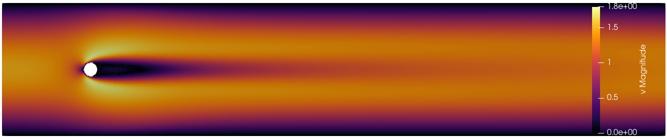
Figure 1: Snapshot of magnitude of the steady-state Navier-Stokes velocity solution in the considered setup.

As the control input, we consider a modulation the input velocity around its reference value. As the observation, we consider a single output $y_{p}$ of the pressure or the single output $y_{v}$ of the sum of the two velocity components averaged over a square domain of area $d^{2}$ located $10d$ behind the cylinder in the wake, where $d$ is the cylinder diameter.

The spatial discretization is obtained by Taylor-Hood piecewise quadratic/piecewise linear finite elements on an unstructured triangulation of the domain which results in around 42000 degrees of freedom for the velocity and 5000 degrees of freedom for the pressure.

The linearized model is obtained from linearizing the system about the corresponding steady-state solution. Thus, the obtained input/output map models the linear response to a changing input velocity in the measurements in the wake; see Fig. 2 for an illustration of the response in time domain. For the presented results on transfer function interpolation, we consider the $y_{p}$ output only, i.e.

$$H_{\mathsf{OS}}(s):=\mathcal{C}_{p}(s\mathcal{E}-\mathcal{A})^{-1}(\mathcal{B}_{1}+s\mathcal{B}_{2}),$$ (31)

with $\mathcal{C}_{p}=\begin{bmatrix}0&C_{p}\end{bmatrix}$.

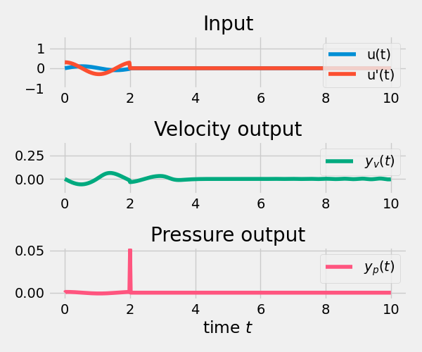
Figure 2: Time-domain linear response of the Oseen system for a test output set to zero for $t\geq 2$. Notably, and in line with the theory, the resulting impulse is observed in the pressure output $y_{p}$ but not in the velocity output $y_{c}$.

5.4 Numerical Results

For further reference, we denote the Antoulas-Anderson approach with polynomial terms (see Sec. 4.1) by poly-AAand the Loewner with explicit matching by (see Sec. 3.2) by poly-Loewner.

We investigate the performance of the poly-AA approach for the MSD and the Oseen example by comparing to a plain Loewner interpolation and the Loewner approach with explicit identification of the constant and the linear term in Sec. 3.2. The parameters for the approximations are chosen as follows:

• For determining the polynomial part in poly-Loewner, we consider the range $[10^{7}j,\,10^{9}j]\subset j\mathbb{R}$ and 20 or 10 for the MSD or Oseen example, respectively, evenly (on the logarithm-scale) distributed interpolation points.

• For determining the proper part in the plain Loewner (and the poly-Loewner), we consider 200 or 40 interpolation points (for MSD or Oseen respectively) evenly log-distributed on $[10^{-2}j,\,10^{4}j]\subset j\mathbb{R}$.

• The order $r$ of the identified is inferred by truncating all singular values smaller than the relative tolerance $10^{-10}$.

• To compute the poly-AA interpolation, for both setups, we used 120 interpolation points, defined as 48 and 12 left and right interpolation points evenly distributed on $[10^{-3}j,\,10^{6}j]\subset j\mathbb{R}$ plus their complex conjugates.

The simulation results are plotted in Fig. 3 (MSD example) and Fig. 4 (Oseen example).

In both examples, the frequency response of the full model and approximations are visually indistinguishable. The plots of the relative errors,, however, reveal the qualitative difference between the plain Loewner approach (which does not capture the linear behavior that dominates for high frequencies) and poly-Loewner and poly-AA as well as quantitative differences between poly-Loewner and poly-AA. While the good performance of poly-AA in the low-frequency regime (and the indifferent performance in the mid-frequency range) are likely be explained by the number and choice of interpolation points, we attribute the reliably worse performance of poly-AA for high-frequencies to the all-at-once determination of proper and non-proper components (cp. Eq. (24)) of the transfer function.

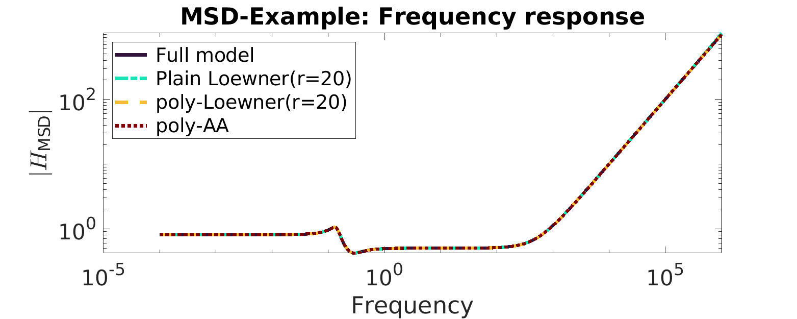
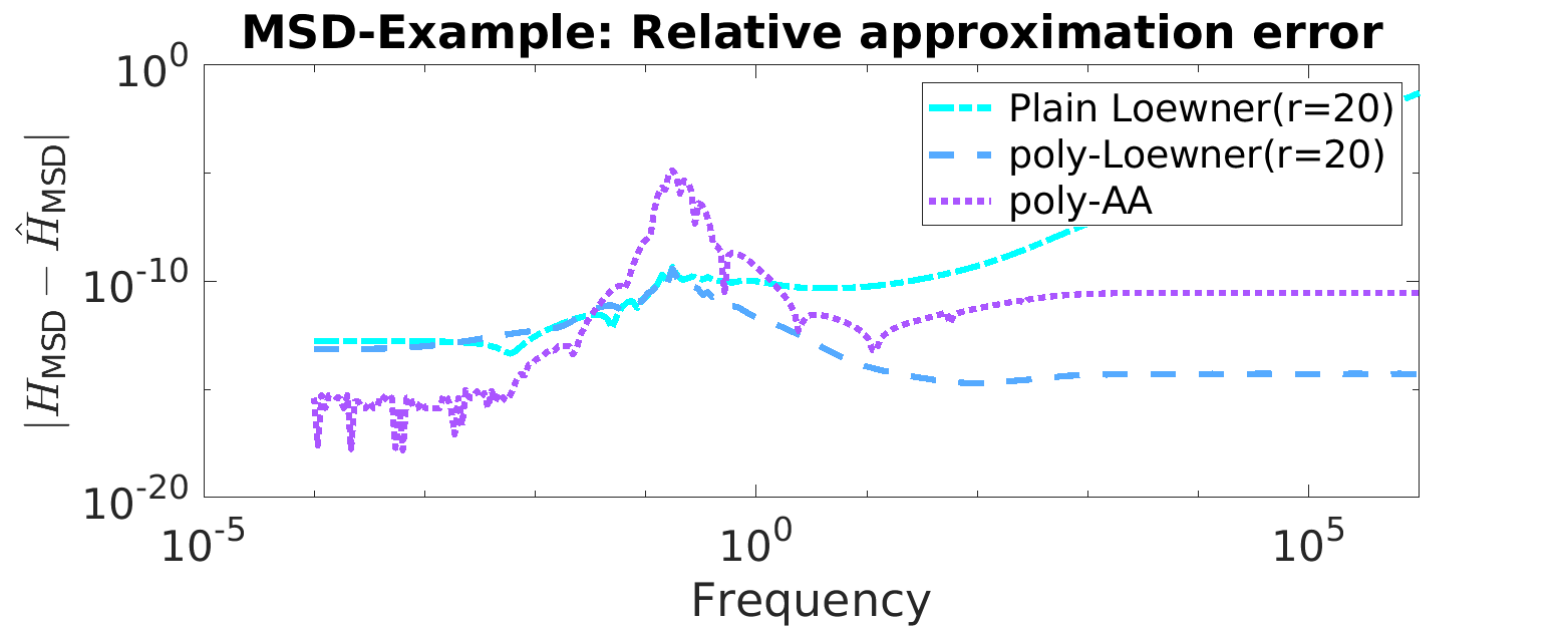
Figure 3: Frequency responses of the MSD full order model and the interpolations (top) and the relative errors (bottom).

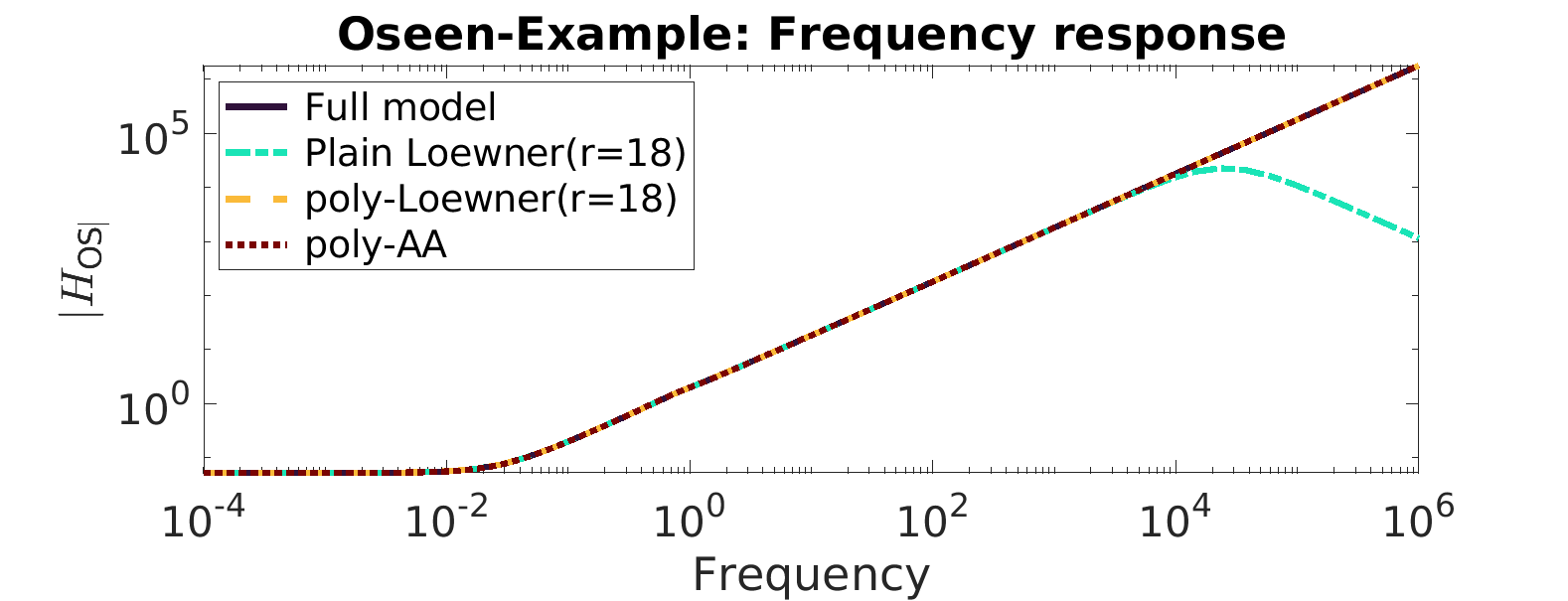
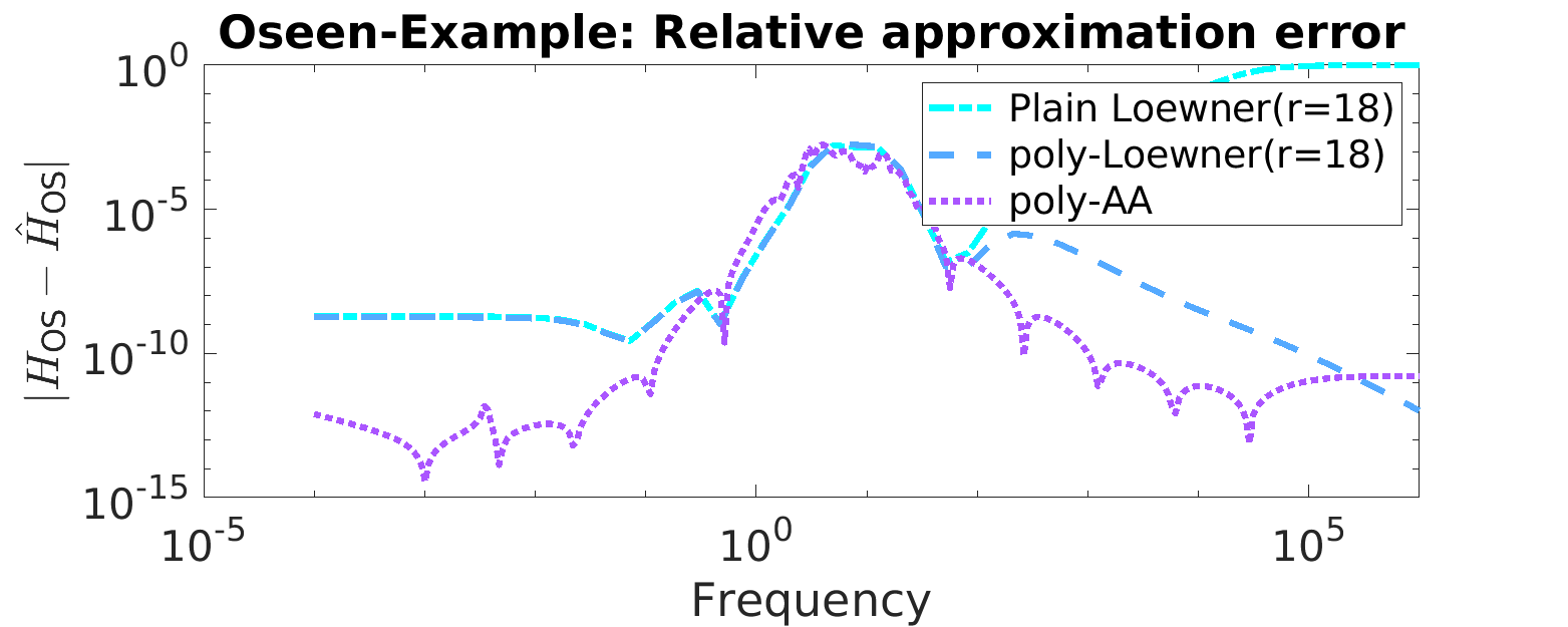
Figure 4: Frequency responses of the Oseen full order model and the interpolations (top) and the relative errors (bottom).

Code Availability

The linear system data (in the form of a .mat file) and the scripts that were used to obtain the presented numerical results are available for immediate reproduction from doi:10.5281/zenodo.10058537 under a CC-BY license.

6 Conclusion

We have proposed a variant of Loewner-based system identification based on the Antoulas-Anderson algorithm but with free parameters to account for non-proper parts. In this approach, polynomial parts of the transfer function are implicitly covered, which is advantageous over explicit treatments of the polynomial parts that requires data points at sufficiently large frequencies. As a drawback of the implicit realization, the determination through, say, singular value decompositions, gives little error control on the individual coefficients and, thus, lead to a larger approximation error in the high frequency range. On the other hand, the equal treatment of all interpolation points gives way to consider adaptive versions of the poly-AA approach as in the adaptive Antoulas-Anderson algorithm; see [16]. Another future investigations will concern extensions of the poly-AA approach to possibly higher polynomial terms.

References

- [1] A. C. Antoulas, S. Lefteriu, and A. C. Ionita, “A tutorial introduction to the Loewner framework for model reduction,” Model Reduction and Approximation: Theory and Algorithms, vol. 15, p. 335, 2017.
- [2] C. C. Pantelides, D. Gritsis, K. R. Morison, and R. W. H. Sargent, “The mathematical modelling of transient systems using differential-algebraic equations,” Computers & chemical engineering, vol. 12, no. 5, pp. 449–454, 1988.
- [3] V. Mehrmann and T. Stykel, “Balanced truncation model reduction for large-scale systems in descriptor form,” in Dimension Reduction of Large-Scale Systems, P. Benner, V. Mehrmann, and D. C. Sorensen, Eds., vol. 45. Springer-Verlag, Berlin/Heidelberg, Germany, 2005, pp. 83–115.
- [4] P. Kunkel and V. Mehrmann, Differential-algebraic equations: analysis and numerical solution. European Mathematical Society, 2006, vol. 2.
- [5] T. Stykel, “Gramian-based model reduction for descriptor systems,” Math. Control Signals Systems, vol. 16, no. 4, pp. 297–319, 2004.
- [6] T. Reis and T. Stykel, “Positive real and bounded real balancing for model reduction of descriptor systems,” Internat. J. Control, vol. 83, no. 1, pp. 74–88, 2010.
- [7] P. Benner and T. Stykel, “Model order reduction for differential-algebraic equations: A survey,” in Surveys in Differential-Algebraic Equations IV, ser. Differential-Algebraic Equations Forum, A. Ilchmann and T. Reis, Eds. Cham: Springer International Publishing, Mar. 2017, pp. 107–160.
- [8] A. J. Mayo and A. C. Antoulas, “A framework for the solution of the generalized realization problem,” Linear Algebra Appl., vol. 425, no. 2-3, pp. 634–662, 2007.
- [9] A. C. Antoulas and B. D. O. Anderson, “On the scalar rational interpolation problem,” IMA J. Math. Control. Inf., vol. 3, no. 2-3, pp. 61–88, 1986.
- [10] I. V. Gosea, Q. Zhang, and A. C. Antoulas, “Preserving the DAE structure in the Loewner model reduction and identification framework,” Adv. Comput. Math., vol. 46, no. 3, 2020.
- [11] A. C. Antoulas, I. V. Gosea, and M. Heinkenschloss, “Data-driven model reduction of the Oseen equations using the Loewner framework,” in Progress in Differential-Algebraic Equations II, ser. Differential-Algebraic Equations Forum, S. Grundel, T. Reis, and S. Schöps, Eds. Springer, 2020, pp. 185–210.
- [12] M. I. Ahmad, P. Benner, P. Goyal, and J. Heiland, “Moment-matching based model reduction for Navier-Stokes type quadratic-bilinear descriptor systems,” Z. Angew. Math. Mech., vol. 97, no. 10, pp. 1252–1267, 2017.
- [13] P. Benner and J. Heiland, “Time-dependent Dirichlet conditions in finite element discretizations,” ScienceOpen Research, pp. 1–18, 2015.
- [14] D. S. Karachalios, I. V. Gosea, and A. C. Antoulas, “The Loewner framework for system identification and reduction,” in Model Order Reduction: Volume I: System-and Data-Driven Methods and Algorithms. De Gruyter, 2021, pp. 181–228.
- [15] B. Gustavsen and A. Semlyen, “Rational approximation of frequency domain responses by vector fitting,” IEEETransPD, vol. 14, no. 3, pp. 1052–1061, 1999.
- [16] Y. Nakatsukasa, O. Sète, and L. N. Trefethen, “The AAA algorithm for rational approximation,” SIAM Journal on Scientific Computing, vol. 40, no. 3, pp. A1494–A1522, 2018.