Emergence of order from chaos through a continuous phase transition in a turbulent reactive flow system

Abstract

As the Reynolds number is increased, a laminar fluid flow becomes turbulent, and the range of time and length scales associated with the flow increases. Yet, in a turbulent reactive flow system, as we increase the Reynolds number, we observe the emergence of a single dominant time scale in the acoustic pressure fluctuations, as indicated by its loss of multifractality. Such emergence of order from chaos is intriguing and has hardly been studied. We perform experiments in a turbulent reactive flow system consisting of flame, acoustic, and hydrodynamic subsystems interacting nonlinearly. We study the evolution of short-time correlated dynamics between the acoustic field and the flame in the spatiotemporal domain of the system. The order parameter, defined as the fraction of the correlated dynamics, increases gradually from zero to one. We find that the susceptibility of the order parameter, correlation length, and correlation time diverge at a critical point between chaos and order. Our results show that the observed emergence of order from chaos is a continuous phase transition. Moreover, we provide experimental evidence that the critical exponents characterizing this transition fall in the universality class of directed percolation. Our study demonstrates how a real-world complex, non-equilibrium turbulent reactive flow system exhibits universal behavior near a critical point.

I INTRODUCTION

The spontaneous emergence of order from a chaotic turbulent state in the form of self-sustained periodic oscillations is encountered frequently in non-equilibrium systems. Examples of such spontaneous oscillations include birdsong, whistling, and the sounds of woodwinds, which are very pleasant [1, 2, 3, 4]. However, within engineering systems, uncontrolled oscillations are highly undesirable as they can frequently result in catastrophic failures of gas transport pipelines [5], rockets and gas turbine engines [6, 7], and bridges, for example, the devastating collapse of the Tacoma bridge [8].

As the Reynolds number (which is the ratio of inertial to viscous force) is increased, the range of time and length scales associated with a fluid flow increases [9, 10]. Yet, in a turbulent reactive flow system, as we increase the Reynolds number, we observe the emergence of a single dominant time scale in the acoustic pressure fluctuations, as indicated by its loss of multifractality [11]. Such emergence of order from chaos is intriguing; moreover, but not studied well. In this regard, we study the emergence of order from chaos in a turbulent thermo-fluid system.

Recent studies in disparate turbulent flow systems reported universal scaling relations during the transition from chaos to order [12, 13]. Such universal power laws during a transition are often associated with a second-order phase transition, specified by the critical exponents [14, 15]. Systems that exhibit the same critical exponents are identified with a universality class. The transition in fluid flows from a laminar to a turbulent state follow the universality class of directed percolation (DP) [16, 17, 18, 19]. Moreover, the synchronization transition in coupled map lattices [20, 21] and cellular automata [22], transition in turbulent liquid crystals [23], and numerous other phenomena [24, 14, 25, 26] fall under the universality class of DP.

In the present work, we perform experiments in a confined turbulent reactive flow system, which consists of flame, hydrodynamic, and acoustic subsystems interacting nonlinearly. As the Reynolds number $Re$ is increased, self-sustained periodic oscillations of large-magnitude emerge in the acoustic pressure as a result of a positive feedback between the different subsystems [27, 28]. This phenomenon, referred to as thermoacoustic instability or combustion instability is a significant concern for the gas turbine power plants, aircraft and rocket engines due to the catastrophic consequences associated with high amplitude acoustic pressure oscillations [6].

We study the evolution of short-time correlated dynamics between the acoustic field and the flame in the spatiotemporal domain of a turbulent reactive flow system. We show that during the emergence of order from a chaotic state, the order parameter, defined as the fraction of correlated dynamics, increases gradually from zero to one. Close to the onset of the transition (critical point), the fluctuations in the order parameter become significant and the variance of the order parameter fluctuations, referred to as susceptibility, exhibits a diverging behavior. We find that the correlations in fluctuations persist longer in the vicinity the critical point. In particular, the correlation length and correlation time diverge according to a power law at the critical point. These measures clearly imply the occurrence of a continuous phase transition from a chaotic to an ordered state even as the Reynolds number is increased. Further, we find that three critical exponents of the transition corresponding to the order parameter and the distribution of intervals between the occurrence of correlated dynamics along space and time fall into the universality class of 2+1 DP. In summary, our work shows that, near the critical point of a continuous phase transition, such a highly nonlinear turbulent system follows universal power laws irrespective of their system-specific details.

II PHASE TRANSITION IN NONEQUILIBRIUM SYSTEMS

In complex systems, a phase represents the collective state of multiple interacting subsystems. When a suitable control parameter is varied, complex systems can exhibit a qualitative change in the collective state of the system. In nonequilibrium systems, these collective, self-organized states emerge and are maintained due to the constant flux of energy [29]. Examples of phase transition in nonequilibrium systems include laminar to turbulent flow transition [16], sleep-wake transition [30], and the emergence of coherent light emission in lasers [31].

DP model typifies phase transition in diverse nonequilibrium systems [14]. This model describes the spread of activity through contact processes, such as the spreading of an epidemic in a community or the spread of forest fires [14]. If the spreading probability $p$ is less than a critical value ($p_{c}$), the system evolves to a state with no activities in the system dynamics. As the spreading probability increases, for $p>p_{c}$, the activity exhibits a percolation phase transition [14].

Order parameter ($\rho$) quantifies the density of active sites in the system during the stationary state. During the DP phase transition, the system exhibits critical scaling behavior near the percolation threshold [14, 32]. The order parameter ($\rho$) exhibits a power law $\rho\sim\epsilon^{\beta}$ with an exponent $\beta$, where $\epsilon=p-p_{c}$ is the distance from the critical point ($p_{c}$) and $\rho$ is the density of the active sites after the system reaches a steady state.

We denote the interval between the consecutive active sites in space as $\ell$, at a time instant. Similarly, the duration between the consecutive active instances is denoted as $\tau$ at a spatial location. These intervals between the occurrences of activities are defined as inactive intervals. The probability distributions ($N$) of inactive time intervals ($\tau$) and length intervals ($\ell$) exhibit power law with $N(\ell)\sim\ell^{-\mu_{\parallel}}$ and $N(\tau)\sim\tau^{-\mu_{\perp}}$ at the critical point of the DP phase transition [14]. The critical behavior associated with the universality class of DP is characterized by specifying the power law exponents $\beta$, $\mu_{\parallel}$, and $\mu_{\perp}$ [14, 33]. Diverse systems including fluid [34, 18, 24], material [25, 35] and biological systems [36] exhibit the same critical behavior as DP.

III Experiments in a Turbulent reactive flow system

Our experimental setup, the turbulent reactive flow system, consists of a mixing duct, bluff body, combustion chamber, and a settling chamber (Fig. 1). Air is first passed through a settling chamber to reduce fluctuations from the air supply line. The fuel (liquified petroleum gas with a composition of $60\%$ butane and $40\%$ propane) is supplied into the mixing tube through radial injection holes of the central shaft, then mixes with the air from the settling chamber and flows into the combustion chamber. The reactant mixture is ignited using a spark plug attached to the backward-facing step of the combustion chamber. The combustion chamber is a duct of length of 1100 mm and with a square cross-section of 90 mm $\times$ 90 mm. One side of the combustion chamber is a backward-facing step through which the reactant mixture enters the combustion chamber. The other end of the combustion chamber is connected to a rectangular chamber (or decoupler) of size 1000 mm $\times$ 500 mm $\times$ 500 mm, much larger than its cross-section. This rectangular chamber is to isolate the combustion chamber from external ambient fluctuations. For optical access to the combustion chamber, two quartz glass windows of 90 mm $\times$ 360 mm are provided on both side walls. The fundamental mode of the combustion chamber is excited during the emergence of periodic oscillations with a frequency of 160 Hz ($f=c/4L$, $c$ is the speed of sound, and $L$ is the length of the combustor). A circular bluff body of diameter 47 mm and thickness 10 mm fixed at a location 32 mm from the backward-facing step creates a wake flow where the flame is stabilized. The flow rates of air and fuel are separately controlled by mass flow controllers (Alicat scientific MCR series) with an uncertainty of $\pm 0.8\%$ percent of measured reading + $\pm 0.2\%$ of full-scale reading.

Figure 1: The schematic of a bluff body stabilized turbulent reactive flow system comprising fuel and air inlets, a plenum and the combustion chamber. The acoustic pressure is measured using a transducer mounted on the combustion chamber while the heat release rate is measured using CH^∗ chemiluminescence imaging using a high-speed camera, whose field of view is shown in the inset. The spatial region indicated by the dashed line is used for further analysis.

We fix the mass flow rate of fuel at 1.75 g/s and vary the mass flow rate of air from 15.3 g/s to 29.5 g/s. This results in the variation in Reynolds number from $Re=3.9-6.8\times 10^{4}$. Here, the Reynolds number is defined as $Re=\rho\bar{v}D/\mu$, where $\bar{v}$ is the average velocity of the fuel-air mixture entering the combustion chamber, $D$ is the diameter of the bluff body, $\rho$ and $\mu$ are the density and dynamic viscosity of the mixture calculated by considering the variation in the mixture composition as the control parameter is varied [37]. The maximum uncertainty in $Re$ (calculated based on the uncertainty of the mass flow controllers) is $\pm 308$. The experiments at each of the specified values of $Re$ are repeated ten times. Ensemble averaging is performed by combining the results from each of these experiments.

In order to study the emergence of order from chaos, we measure the acoustic pressure fluctuations ($p^{\prime}(t)$) and the spatial distribution of heat release rate fluctuations ($\dot{q}^{\prime}(\mathbf{x},t)$) inside a rectangular region (Fig. 1, 2(e)) of the combustion chamber. The acoustic pressure fluctuations inside the combustion chamber are measured using a piezoelectric pressure transducer (PCB 103B02) mounted 120 mm from the dump plane of the combustion chamber. The pressure transducer is mounted to the wall of the combustion chamber using a T-joint mount. A semi-infinite waveguide of length 10 m and inner diameter 4 mm is connected to the transducer mount to minimize the frequency response of the probe. The pressure transducer has a sensitivity of 223.4 mV/kPa and an uncertainty of $\pm 0.15$ Pa. The acoustic pressure is measured with a sampling frequency of 10 kHz for a duration of 3s. The signals from the piezoelectric pressure transducer were recorded using a data acquisition system (NI DAQ-6346). The chemiluminescence intensity represents the line-of-sight integrated heat release rate distribution [38]. The heat release rate fluctuations are determined from the chemiluminescence images acquired using the high-speed Phantom V12.1 camera outfitted with a CH* filter (a narrow band filter of peak at 435 nm with 10 nm FWHM) along with a 100 mm Carl-Zeiss lens. A region spanning 80 $\times$ 80 $\mathrm{mm}^{2}$ is imaged at a resolution of 520 $\times$ 520 pixels at a sampling rate of 2000 Hz simultaneously with the piezoelectric transducer. We perform a coarse-graining operation by combining 10 $\times$ 10 pixels of the chemilumuniscence images to decrease the noise levels.

Figure 2: Transition from combustion noise to thermoacoustic instability. (a) The amplitude ($p^{\prime}_{\text{rms}}$) and (b) the power spectral density (PSD) of $p^{\prime}$ as a function of $Re$. With an increase in $Re$, there is a gradual increase in the amplitude of oscillations accompanied by the appearance of a dominant frequency in the system response. Representative (c) time series (normalized $p^{\prime}$ and $\dot{q}^{\prime}$) and (d) phase space trajectory for $p^{\prime}$ corresponding to the dynamical states of chaos, intermittency and limit cycle oscillations, indicated in (a). The phase space is reconstructed using time delay ($\tau$) embedding. (e) The distribution of heat heat release rate fluctuation $\dot{q}^{\prime}(\textbf{x},t)$ at the indicated instance in (b).

IV Emergence of order from chaos

Figure 2 shows the dynamics of the turbulent reactive flow system when the Reynolds number is increased from $Re=3.9\times 10^{4}$ to $Re=6.8\times 10^{4}$. Figures 2(a) and 2(b) depict the change in the root-mean-square (r.m.s.) amplitude of the pressure oscillations and the corresponding power spectral density, respectively. The low-amplitude, aperiodic oscillations (Fig.2(c)-i) are identified as high-dimensional chaos [39]. As $Re$ is increased, we notice that the turbulent reactive flow system undergoes a transition from a state of low-amplitude, high-dimensional chaos to a state characterized by high-amplitude periodic acoustic pressure oscillations (Fig. 2(a), Fig. 2(c)-i, ii, iii). The power spectrum, which is broad-band, becomes progressively narrower as $Re$ is increased. At the onset of periodic oscillations, the frequency of the dominant mode of acoustic pressure oscillations is 160 Hz, evident in the amplitude spectrum shown in Fig. 2(e).

The phase space trajectories associated with the acoustic pressure fluctuations reconstructed using Takens embedding theorem [40] are shown in figure 2(d). Corresponding to the state of chaotic fluctuations, the trajectory (Fig. 2(d)-i) appears to fill the phase space with no clearly defined attractor. During the chaotic state, the trajectory of the system often switches between multiple unstable periodic orbits (UPOs), as the trajectory is ejected along the unstable manifold from one UPO and attracted towards the stable manifold of another UPO [41, 42]. The phase space of the chaotic state thus appears haphazard due to the switching between these UPOs (Fig. 2(d)-i).

Upon further increase in $Re$ beyond $5.1\times 10^{4}$, we observe the state of intermittency where bursts of high-amplitude periodic acoustic pressure fluctuations appear amidst epochs of low-amplitude aperiodic acoustic pressure fluctuations (Fig. 2(c)-ii) [43]. During the state of intermittency, the trajectory of the system transits between an inner chaotic region and outer periodic orbits in the phase space of the system dynamics (Fig. 2(d)-ii) [42]. We observe sustained periodic acoustic pressure oscillations (Fig. 2(c)-iii) as we further increase the $Re$ to $6.8\times 10^{4}$. During the emergence of periodic oscillations, the number of unstable periodic orbits decreases and their stability increases. Eventually, the UPOs collapse to form a stable periodic orbit [42], and the system exhibits limit cycle oscillations (Fig. 2(d)-iii).

To compare the flame dynamics to acoustic pressure fluctuations, the time series of heat release rate fluctuation is obtained by summing over the chemiluminescence imaging such that $\dot{q}^{\prime}(t)=\sum_{x,y}\dot{q}(\mathbf{x},t)-\overline{\dot{q}}$, where $\overline{\dot{q}}$ is the mean value of $\dot{q}(\mathbf{x},t)$. The normalized heat release rate fluctuation is overlaid on normalized $p^{\prime}$ to observe their relative time evolution as shown in Fig. 2(c). The normalization of $\dot{q}^{\prime}$ and $p^{\prime}$ is done using their standard deviation values. Further, in figures 2(e)-i, 2(e)-ii, and 2(e)-iii, the heat release rate fluctuations across the spatial field $\dot{q}^{\prime}(\textbf{x},t)$ are shown for the instances marked in Fig. 2(c)-i, 2(c)-ii, and 2(c)-iii respectively. The flame and acoustic subsystems exhibit desynchronized dynamics (Fig. 2(c)-i) and the values of heat release rate fluctuations remains very small (Fig. 2(e)-i) during the state of chaos. The flame and the acoustic field exhibit synchronized dynamics when the turbulent reactive flow system exhibits sustained periodic limit cycle oscillations (Fig. 2(c)-iii) [44, 45, 46]. During this state, the heat release rate fluctuations has large values distributed throughout the reaction field (Fig. 2(e)-iii). The heat release rate distribution for the state of intermittency is shown in figure 2(e)-ii. In a previous study, Mondal et. al [46] showed that synchronous and asynchronous dynamics between $p^{\prime}$ and $\dot{q}^{\prime}(\mathbf{x},t)$ co-exist during the state of intermittency. Thus, the turbulent reactive flow system clearly shows the emergence of periodic oscillations from a chaotic state through intermittency while we increase the Reynolds number.

Figure 3: Space-time ($\textbf{x}-t$) diagram illustrating the phase transition from chaos to order. Panels (a-c) correspond to the state of chaos, intermittency and limit cycle oscillations, as indicated in Fig. 2a. Regions of ordered activity, identifying the existence of high correlation between acoustic pressure and the heat release rate fluctuations, is visualized with the color scheme and is delineated from regions of disordered activity using (3). For the chaotic state (a), the regions of ordered activity are very small and disconnected. At the critical point associated with the state of intermittency (b), small ordered regions grow and form giant ordered regions. The slice in $X-X^{\prime}$ and $T-T^{\prime}$ shows the appearance and disappearance of giant cluster in space and time. Inactive interval distribution are labeled in space $\ell_{y}$ and time $\tau$. During the state of limit cycle oscillations (c), order percolates throughout the spatiotemporal domain.

V Emergence of order through a continuous phase transition

We quantify the transition by determining the short-time window adjusted cross-correlation between $p^{\prime}(t)$ and $\dot{q}^{\prime}(\mathbf{x},t)$. The acoustic pressure fluctuations remain spatially uniform within the region of interest (Fig. 1) since the reaction zone is small in comparison to the acoustic length scales which are of the same order as the length of the combustion chamber (refer to Supplemental Material Sec. III [47]). Further, since the transition occurs through the state of intermittency which features localized bursts of periodic fluctuations, a short-time window is used to capture the intermittent features. The time-shifted cross-correlation is defined as

$$\mathcal{R}(\mathbf{x},t,\tau_{i})=\int_{t}^{t+W}p^{\prime}(t_{1})\dot{q}^{\prime}(\mathbf{x},t_{1}+\tau_{i})dt_{1}.$$ (1)

Here, the correlation is calculated over a short-time window of time $W$, for different time shift values ranging from $\tau_{i}=-T/2$ to $+T/2$, where $T$ is the time period of the dominant acoustic pressure oscillations. If $W$ is too short, the correlation becomes meaningless and depict significant level of fluctuations, whereas, if it is too large, it fails to distinguish short-bursts of periodic oscillations. In Appendix A, we show that a window of size $W=4T$ adequately captures the correlations during intermittency, and so we consider $W=4T$ throughout our calculations.

Finally, the short-time window adjusted correlation is obtained as

$$R(\textbf{x},t)=\max_{\tau_{i}}\{\mathcal{R}(\textbf{x},t,\tau_{i})\}.$$ (2)

For aperiodic, uncorrelated fluctuations, the cross-correlation values ($\mathcal{R}$) are very small irrespective of the time shift (Fig. 8(b)-ii). On the other hand, if both the time series are periodic or correlated, the cross-correlation value ($\mathcal{R}$) attains a high value for a time shift value corresponding to the phase difference between the two time series (Fig. 8(b)-i). We introduce the state variable ($S$), defined as

$$S({\textbf{x},t})=\begin{cases}1&\text{if $R\geq R_{\text{Th}}$,}\\ 0&\text{otherwise,}\end{cases}$$ (3)

to distinguish between correlated and uncorrelated dynamics. We set a threshold value of $R_{\text{Th}}(\mathbf{x},t)=0.6$ for all cases. The presented results are independent of the value of $R_{\text{Th}}$ (refer to Appendix B).

The scalar variable $S$ classifies the existence of ordered or disordered activity at a given space-time location ($\textbf{x}-t$). Thus, $S=0$ indicates a disordered activity arising due to turbulence resulting in uncorrelated dynamics, whereas $S=1$ indicates ordered activity in the form of periodic fluctuations, resulting in very high correlations.

Figure 4: Variation of the (a) $\langle\rho\rangle$ and the susceptibility $\langle\chi\rangle$ as a function of the distance from the critical point, $\epsilon={(Re-Re_{c})}/{Re_{c}}$. (b) Scaling of the order parameter $\rho_{n}$ with an exponent $\beta=0.55\pm 0.12$. The scaling associated with the universality class of $2+1$ directed percolation ($\beta_{DP}=0.583$) is also shown by the dashed line as a reference. (c) power law scaling of $\chi$ as a function of $|\epsilon|$ as critical point is approached from either side, with the exponents $\gamma^{\prime}_{\epsilon<0}=0.93\pm 0.18$ and $\gamma_{\epsilon>0}=0.95\pm 0.35$. Ensemble averaging is performed to obtain the uncertainty in the power law exponents by considering $90\%$ confidence interval around the mean; all error bars correspond to standard deviation.

The regions of ordered activity (ordered regions) show a percolation phase transition in space and time as $Re$ is increased (Fig. 3). The evolution of (ordered regions) for the state of chaos, intermittency and limit cycle are shown in figures 3(a), 3(b), and 3(c) respectively. During the state of chaos, ordered regions are small and scattered, and they appear and disappear erratically (Fig. 3(a)). However, during the state of intermittency, we observe that some randomly occurring ordered regions grow and form a giant ordered region that spans the entire spatial domain. The giant ordered region formed at an instant ($T-T^{\prime}$ plane) is shown in Fig. 3(b). The giant ordered region formed is not sustained long enough; soon it breaks down and disappears (Fig. 3(b)). The formation and the breakdown of the giant ordered region are visible in the slice $X-X^{\prime}$ of the spatiotemporal domain shown in Fig. 3(b). During the state of limit cycle oscillations, we find that ordered activity percolates in space and time (Fig. 3(c)).

In summary, as $Re$ is increased, we observe a phase transition from a predominantly disordered state where ordered regions appearing are small and scattered, to a dominant ordered state where the regions of ordered activity percolate throughout space and time.

VI Critical exponents of the percolation phase transition

VI.1 Order parameter, susceptibility and inactive interval distribution

Having clarified visually, we quantify the characteristics of phase transition next. The variable $S$ allows us to further quantify the system in terms of the order parameter and related statistics. The order parameter ($\rho$) is a measure of the degree of ordered activity in the system dynamics. The order parameter is defined as the fraction of sites depicting order at a given time instant. Formally, it can be expressed as

$$\rho(t)=\frac{1}{L^{2}}\sum_{x_{i},y_{j},t}S(x_{i},y_{j},t),$$ (4)

where, $L^{2}$ is the overall domain size and the summation spans across the entire spatial domain. Consequently, the mean order parameter is expressed as: $\langle\rho\rangle=\langle 1/N\sum_{t}\rho(t)\rangle$, where $N$ is the total number of points in the time series. Here, and in the following, $\langle\cdot\rangle$ implies an ensemble average over the ten realizations of the experiments at each control parameter. Kindly refer to Appendix A for more details on the ensemble averaging.

In real systems, the value of the order parameter at the critical point $\rho(\epsilon=0)\neq 0$ due to the finite size of the system [48]. Thus, it is important to introduce the normalization $\rho_{n}=[\langle\rho\rangle-\langle\rho\rangle_{0}]/[1-\langle\rho\rangle_{0}]$ such that $\rho_{n}$ varies between 0 and 1, so as to accurately obtain the power law. We further define the variance of the order parameter which is referred to as the susceptibility, as

$$\langle\chi\rangle=\left\langle\frac{1}{N}\sum_{t}\left[\rho^{2}(t)-(\bar{\rho})^{2}\right]\right\rangle,$$ (5)

Finally, close to the critical point, the normalized mean order parameter ($\rho_{n}$) and susceptibility $\chi$ are well-known to scale as power law [49]:

$$\rho_{n}\sim\epsilon^{\beta},\qquad\langle\chi\rangle\sim\epsilon^{\gamma},$$ (6)

where, $\epsilon=(Re-Re_{c})/Re_{c}$ and $\beta$ and $\gamma$ are the respective scaling exponents.

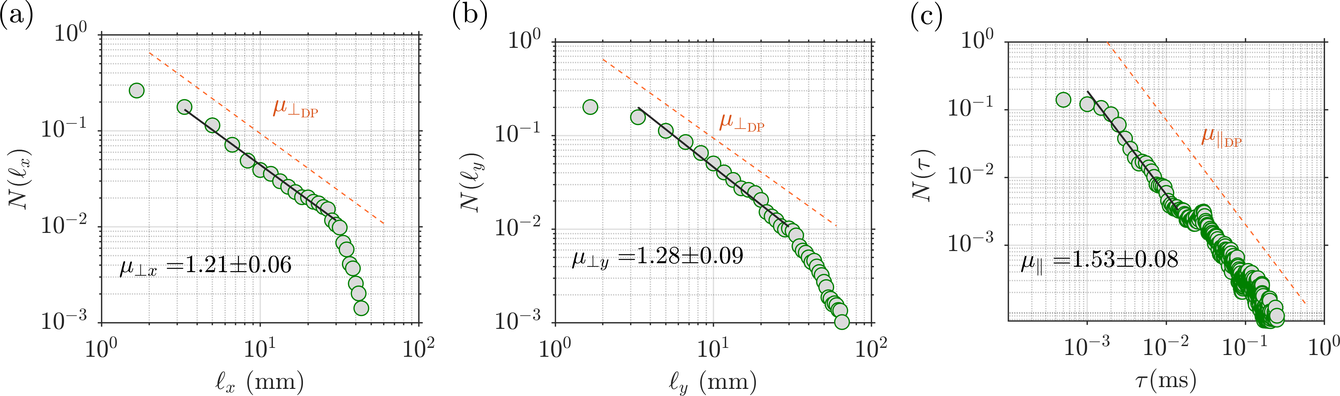
Figure 5: power law scaling of the probability distribution $N$ of inactive intervals between two regions of ordered activity in (a,b) space ($\ell_{x},\ell_{y}$) and in (c) time ($\tau$) close to the critical point $\epsilon\approx 0$. The observed scaling behavior closely follows the power law scaling associated with the inactive interval distribution of $2+1$ DP (dashed line).

Figures 4 presents the scaling behavior of the order parameter and susceptibility as a function of $\epsilon$. We find that the ensemble average of the mean order parameter $\langle{\rho(t)}\rangle$ gradually increases from close to $\langle\rho\rangle=0$ far from the critical point to $\langle\rho\rangle=1$ during the transition (Fig. 4(a)). Between order and chaos, we observe that the variance of the order parameter fluctuations becomes extremely significant and diverges (Fig. 4(a)). Such a divergence clearly reveals that the system is approaching a critical point and an impending phase transition.

Next, we observe that the normalized order parameter $\rho_{n}$ increases following the power law: $\rho_{\mathrm{n}}\sim\epsilon^{\beta}$ with the exponent $\beta=0.55\pm 0.12$ in the vicinity of the critical point (Fig. 4(b)). This scaling closely follows the scaling behavior of directed percolation. Further, we find that the susceptibility diverges with a power law: $\langle\chi\rangle\sim\epsilon^{-\gamma}$ with the exponents $\gamma=0.95\pm 0.35$ for $\epsilon>0$ and $\gamma^{\prime}=0.93\pm 0.18$ for $\epsilon<0$ respectively (Fig. 4(c)). Thus, the observed transition is continuous with susceptibility exhibiting a diverging behavior between chaos and order.

Here, and in what follows next, the uncertainty in the value of scaling exponents is obtained by considering the $90\%$ confidence interval around the mean from the ensemble of realizations of the experiments. Similarly, the vertical and horizontal error bars are calculated based on the standard deviation from the ensemble mean values of normalized order parameter and $\epsilon$ values within the bins of size $\delta\epsilon=0.025$.

Next, we quantify the critical exponents associated with the inactive interval distribution. Inactive interval refers to the duration ($\tau$) or separation ($\ell_{x},\ell_{y}$) between two consecutive ordered activities, as illustrated in Fig. 3(b). We obtain the probability distribution of inactive interval distribution in space [$N(\ell_{x}),N(\ell_{y})$] and time [$N(\tau)$] from the percolation diagram, as highlighted in Fig. 3. The resulting distributions are plotted in Fig. 5. We find that close to the critical point of the transition, the inactive interval distributions also show clearly defined power law scaling of the form:

$$N(\ell_{x})\sim\ell_{x}^{\mu_{\perp x}},\enspace N(\ell_{y})\sim\ell_{y}^{\mu_{\perp y}},\enspace N(\tau)\sim\tau^{\mu_{\parallel}}$$ (7)

We find that the exponents describing the inactive intervals are $\mu_{\perp x}={-1.21\pm 0.06}$, $\mu_{\perp y}={-1.28\pm 0.09}$, and $\mu_{\parallel}={-1.53\pm 0.08}$. Such power law behaviors in the distribution of inactive intervals signify the scale invariant nature of the system at the critical point. We also find that the critical exponents corresponding to the inactive interval distributions [$N(\tau)$, $N({\ell_{x}})$ and $N({\ell_{y}})$] fall into the universality class of 2+1 DP (see Supplemental Material Sec. II [47]).

VI.2 Scaling of correlation length and time

In complex systems, significant correlations arise in space and time due to the interaction between the constituent subsystems. For this, we define the two-point correlation function for the scalar field $S(\textbf{x},t)$, which quantifies how the state of the system at two points separated by duration $\tau$ and space $\textbf{r}=[r_{x},r_{y}]^{T}$ are inter-related. Formally,

$$g(\tau) =\langle[S^{\prime}(\textbf{x},t)S^{\prime}(\textbf{x},t+\tau)]\rangle,$$ (8)

$$g(\textbf{r}) =\langle[S^{\prime}(\textbf{x},t)S^{\prime}(\textbf{x+r},t)]\rangle.$$ (9)

Here, $S^{\prime}=S-\langle S\rangle$ and the averaging $\langle f(\textbf{x},t)\rangle=1/NL^{2}\sum_{x,y,t}f(\textbf{x},t)$ is defined over space and time. The correlation is further normalized by its value at the origin, or the auto-correlation, $g(\tau=0)$, $g(\textbf{r}=0)$ such that we have: $G(\tau)=g(\tau)/g(\tau=0)$ and $G(\textbf{r})=g(\textbf{r})/g(\textbf{r}=0)$.

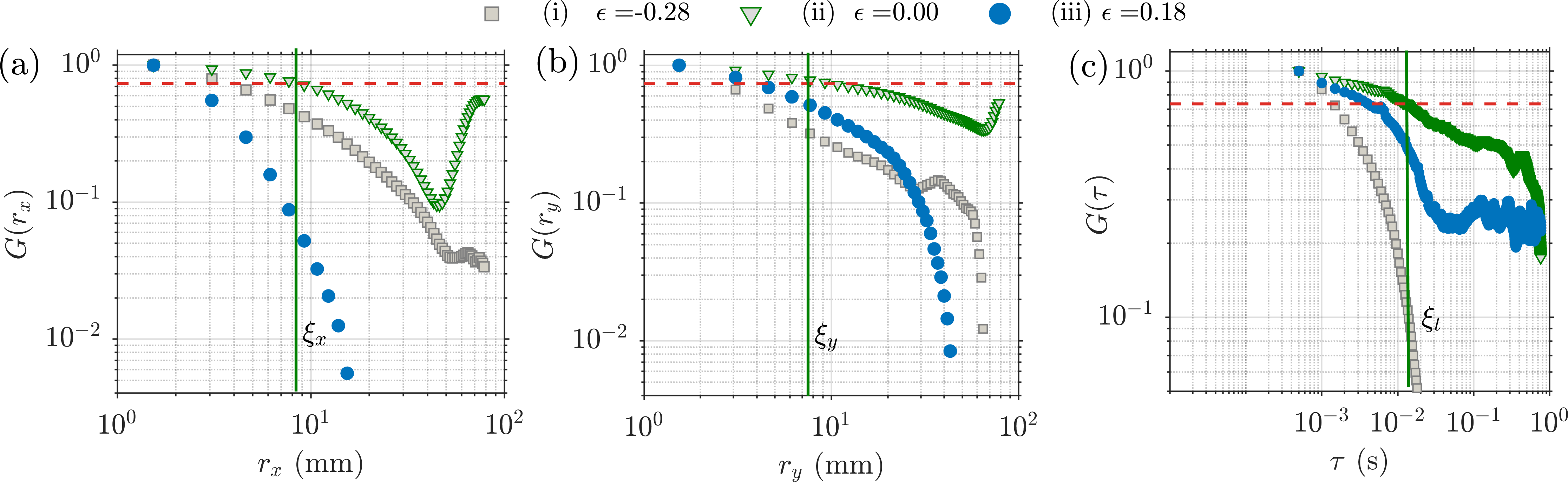
Figure 6: (a-c) Normalized correlation function $(G)$ along $x$, $y$ and $t$ are shown for three $\epsilon$ values $\epsilon=-0.28$ (s), (ii) $\epsilon=0$ (green) and (iii) $\epsilon=0.19$ (blue) in the log-log scale. The correlation length ($\xi_{x,y}$) and the correlation time ($\xi_{\tau}$) have also been identified as the length or time of cross $G=2/e$ (dashed line). Correlation $G$ persists the longest at the critical point $\epsilon=0$.

The plot for normalized correlation functions ($G$) along $x,~{}y$, and $t$ for three different values of $\epsilon$, before the critical point, very close to the critical point, and after the critical point ($\epsilon=-0.28$, $0$, and $0.18$) are shown in Fig. 6(a-c). As the distance (duration) between the spatial locations (instances) increases, the correlation function decreases. However, in the vicinity of the critical point, $G(r_{x})$, $G(r_{y})$, and $G(\tau)$ decay much more slowly (see Supplemental Material Sec. III [47] for more details). Such persistence and slow decay imply that the correlation lengths and times become large due to the scale invariant nature of clusters of ordered activity arising in the system.

The correlation time ($\xi_{\tau}$) and length ($\xi_{x,y}$) are then defined as the time or separation at which the correlation function crosses $G=2/e$ [50, 51, 52] (see Supplemental Material Sec. III [47] for more details). This is also indicated in Fig. 6(a-c). The correlation time ($\xi_{\tau}$) or the correlation length ($\xi_{x}$, $\xi_{y}$ along $x$, $y$ respectively) is a measure of how far the correlation persists in the system. The variation in correlation length and correlation time are shown in Fig. 7(a-c). We find that $\xi_{\tau}$, $\xi_{x}$ and $\xi_{y}$ increase in a power law manner as we approach the critical point from either side. Thus, for $\epsilon>0$, we obtain the power law exponents $\xi_{\tau}=0.68\pm 0.21$, $\xi_{x}=0.46\pm 0.11$, and $\xi_{y}=0.31\pm 0.08$. Similarly, for $\epsilon<0$ are $\xi_{\tau}=0.77\pm 0.12$, $\xi_{x}=0.31\pm 0.08$, and $\xi_{y}=0.47\pm 0.10$), respectively. Such growing correlation time and length are characteristics of second-order phase transition [49].

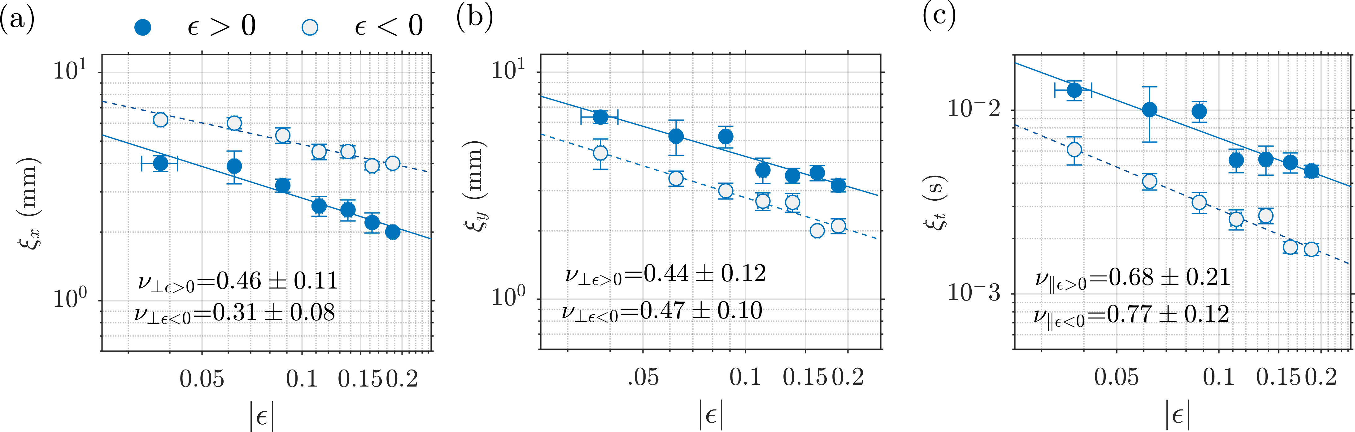
Figure 7: Log-log plot showing the variation of the (a,b) correlation length ($\xi_{\perp x}$, $\xi_{\perp y}$) and the (c) correlation time ($\xi_{\parallel}$) with respect to $\epsilon$. A power law of the form $\xi\sim|\epsilon|^{-\nu}$ is fitted with observed values of the correlation length and time for $|\delta\epsilon|<0.16$. We observe that the correlation length and duration grow as a power law, as the system approaches the critical point from either side of the critical point.

VII DISCUSSION

Table 1: Critical exponents obtained for the percolation phase transition in the turbulent reactive flow system.

Exponent	Turbulent reactive flow system	2+1 DP
$\beta$	$0.55\pm 0.12$	$0.583$
$\mu_{\parallel}$	$1.53\pm 0.08$	$1.549$
${\mu_{\perp}}^{\text{c,}}$	$1.21\pm 0.06$ ($1.28\pm 0.09$)	$1.204$
${\nu_{\parallel}}^{\text{b}}$	$0.68\pm 0.21$	$1.295$
${\nu_{\perp}}^{\text{b,d}}$	$0.46\pm 0.11$ ($0.44\pm 0.12$)	$0.733$
$\gamma^{\text{b}}$	$0.95\pm 0.35$	$0.2998$

We conducted experiments in a confined turbulent reactive flow system and studied the evolution of the correlated dynamics between the flame and the acoustic subsystems. We observe that the correlated dynamics undergo a percolation phase transition during the emergence of order from chaos. We find that the order parameter gradually increases from zero to one during the percolation phase transition. The correlation time, correlation length, and susceptibility diverge at the critical point of the transition. The critical exponents that characterize this phase transition are listed in Table 1. We find that close to the critical point, the critical exponents corresponding to the normalized order parameter ($\beta$), and the distribution of inactive intervals along space ($\mu_{\perp x}$, and $\mu_{\perp y}$) and time $\mu_{\parallel}$ fall into the universality class of 2+1 DP. We also observe that the choice of threshold values for the short-time window correlations ($R_{\mathrm{max}}$) used for identifying correlated dynamics does not affect our results (refer Fig. 9 in Appendix B for details). Our results suggest that the critical phenomenon we studied belongs to the universality class of DP.

The DP conjecture states that, the transition in a system with a unique absorbing state, short-range dynamic rules, and the absence of special attributes such as the existence of inhomogeneities belongs to the universality class of directed percolation [53]. In experimental systems, a pure absorbing state is challenging to achieve due to the inherent fluctuations in the system [33]. Moreover, this limitation makes it hard to identify systems that belong to the universality class of DP through experimental realizations [33]. Despite these difficulties, a handful of experimental studies showed that the transition in turbulent liquid crystals [23], the transition in ferrofluids [26], the onset of the Leidenfrost effect [24], and the transition from laminar to turbulent state in fluid mechanical systems [18, 34] fall under the universality class of DP.

The reactant mixture entering the combustion chamber burns while being convected downstream; and the propagation of these reactions (burning reactants) is analogous to a contact process [54]. The dynamics of the ordered activities are governed by this contact processes as well as the fluctuations induced due by the global acoustic field. The turbulent reactive flow system does not strictly follow the DP conjecture. A unique absorbing state is absent during the chaotic state in the turbulent reactive flow system since small ordered activities erratically appear and disappear for $\epsilon<0$. The inherent fluctuations in the system due to turbulence could be the reason for not observing a unique absorbing state [33]. However, we observe that three critical exponents ($\beta$, $\mu_{\perp}$, and $\mu_{\parallel}$) fall into the universality class of DP. The robustness of the universality class of DP under the relaxation of the DP conjecture [55, 56, 57, 58] could be why we still observe the critical exponents to be the same as the universality class of DP.

Numerical studies on many spatially extended systems suggest that synchronization transition could belong to the universality class of DP [59, 60, 20, 61, 22, 21, 62]. Future studies on identifying the synchronization activities between the flame and acoustic subsystems and its spatiotemporal evolution will help to characterize the synchronization transition in the turbulent reactive flow systems.

The universality class of DP typifies phase transition observed in a wide variety of physical systems [14]. Further, the universality in statistical models provides insights into how the correlated dynamics (between the subsystems) in diverse systems such as turbulent flow [34, 18] and biological systems [36, 63, 64] are connected, irrespective of their microscopic system details. The statistical analysis based on interdependent fluctuations between the interacting subsystems could help us gain more insights into emergent phenomena associated with nonequilibrium phase transition in complex systems.

Appendix A Determining window size for obtaining short-time cross-correlation

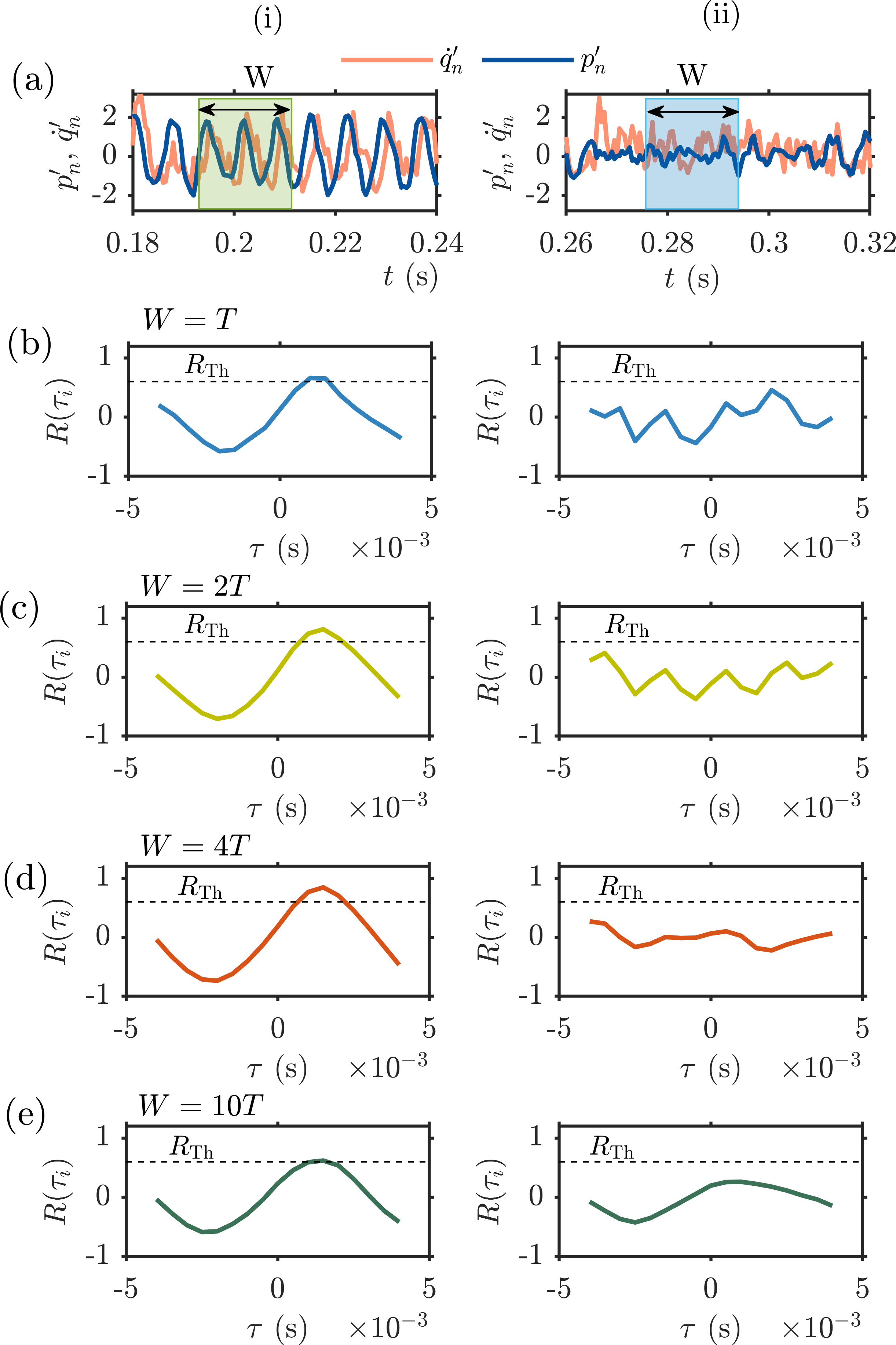
Figure 8: (a-i, a-ii) The normalized acoustic pressure fluctuations and heat release rate fluctuations from a spatial location at $Re=5.13\times 10^{4}$ for two epochs, periodic and aperiodic. The normalization is done using the standard deviation of the fluctuations. Short-time cross-correlation ($R$) for different window sizes of $W$ = $T$, $2T$, $4T$, and $10T$ between $p^{\prime}_{n}$ and $\dot{q}_{n}^{\prime}$ for different lag values ($\tau_{i}$) are calculated for the periodic (column i) and aperiodic (column ii) epochs. The blue dotted line is the threshold ($R_{\text{Th}}=0.6$) for identifying the correlated dynamics.

The short-window adjusted correlation is defined in (1). Clearly, determining $\mathcal{R}$ is important for identifying regions of ordered activity during the state of intermittency and for the subsequent analysis. This requires optimizing the value of the window size $W$ to capture significantly high-correlation values during periodic bursts during intermittency. To this end, the acoustic pressure fluctuations and the heat release rate fluctuations (from a spatial location) at $Re=5.13\times 10^{4}$ for two epochs are shown in Fig. 8(a). The cross-correlation values for a short duration ($W$) with different time-shift values corresponding to periodic (Fig. 8(a)-i) and aperiodic (Fig. 8(a)-ii) acoustic pressure fluctuations are calculated. Different values of the window sizes $W$ are selected for calculating the cross-correlation. If the window is too short, the correlation becomes meaningless, and we observe high fluctuations in $R(\tau_{i})$ (Fig. 8(b)-ii) for different time-shift values. If, on the other hand, the window is too long, features such as short bursts of periodic oscillations during the state of intermittency will not be captured since the value of short-time cross-correlation decreases as the window size increases (Fig. 8(e)-i).

For the aperiodic epoch, the short-time cross-correlation values are small and less than the threshold value of $R_{\text{Th}}=0.6$, irrespective of $\tau_{i}$ values (Fig. 8(d)-ii) for a window size of $4T$. However, during the periodic epoch as shown in Fig. 8(a), the fluctuations in acoustic pressure and heat release rate are almost periodic and the cross-correlation value between them is very high corresponding to a time-shift value equivalent to the phase difference between the fluctuations Fig. 8(d)-i. Hence we select a window size of $4T$ for our analysis.

Appendix B Effect of threshold on the critical exponents

Here we discuss the effect the value of threshold $R_{\text{Th}}$ has on the critical behavior. Figure 9 presents the variation of the value of the observed critical exponents ($\beta,\mu_{\parallel},\mu_{\perp_{x,y}}$) as a function of $R_{\text{Th}}$. We observe that within the range of threshold values from 0.55 to 0.65, the critical exponents values remain nearly the same. Increasing the threshold to a very high value ($R_{\text{Th}}>0.8$) of course leads to an increase in $\beta$ as the scaling becomes much more steeper. Thus, the reported scaling exponents are accurately identified and the choice of $R_{\text{Th}}$ does not affect our results.

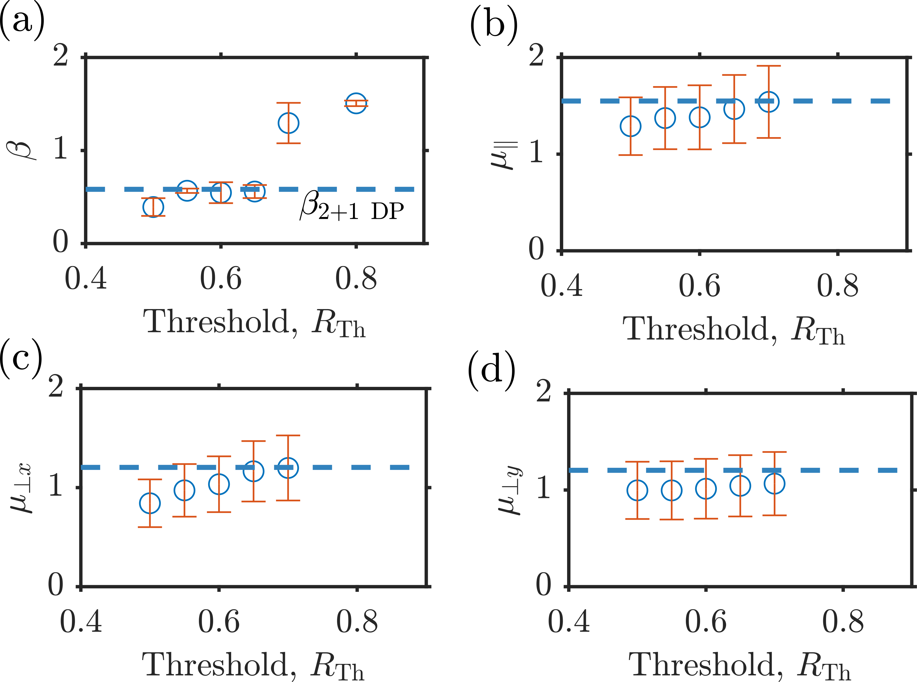
Figure 9: (a-d) The critical exponents $\beta$, $\mu_{\parallel}$, $\mu_{\perp x}$, and $\mu_{\perp y}$ calculated for various threshold values for for identifying the ordered regions. The error bars represent $\pm\sigma$, where the standard deviation $\sigma$ is evaluated across the ensemble of experiments. The reported scaling exponents are remains for same and independent of the choice of the threshold value $R_{\text{Th}}$ between 0.55 to 0.65.

References

- Fee et al. [1998] M. S. Fee, B. Shraiman, B. Pesaran, and P. P. Mitra, The role of nonlinear dynamics of the syrinx in the vocalizations of a songbird, Nature 395, 67 (1998).
- Anderson [1952] A. Anderson, Dependence of pfeifenton (pipe tone) frequency on pipe length, orifice diameter, and gas discharge pressure, The Journal of the Acoustical Society of America 24, 675 (1952).
- Hirschberg et al. [1989] A. Hirschberg, J. Bruggeman, A. Wijnands, and N. Smits, The “whistler nozzle” and horn as aero-acoustic sound sources in pipe systems, Acta Acustica united with Acustica 68, 157 (1989).
- Howe [1975] M. Howe, Contributions to the theory of aerodynamic sound, with application to excess jet noise and the theory of the flute, Journal of Fluid Mechanics 71, 625 (1975).
- Kriesels et al. [1995] P. Kriesels, M. Peters, A. Hirschberg, A. Wijnands, A. Iafrati, G. Riccardi, R. Piva, and J. Bruggeman, High amplitude vortex-induced pulsations in a gas transport system, Journal of Sound and Vibration 184, 343 (1995).
- Fisher et al. [2009] S. C. Fisher, S. A. Rahman, and J. Center, Remembering giant, NASA History Division, Washington, DC, USA (2009).
- Lieuwen and Yang [2005] T. C. Lieuwen and V. Yang, Combustion instabilities in gas turbine engines: operational experience, fundamental mechanisms, and modeling (American Institute of Aeronautics and Astronautics, 2005).
- Green and Unruh [2006] D. Green and W. G. Unruh, The failure of the tacoma bridge: A physical model, American Journal of Physics 74, 706 (2006).
- Tennekes and Lumley [1972] H. Tennekes and J. L. Lumley, A first course in turbulence (MIT press, 1972).
- Pope [2001] S. B. Pope, Turbulent flows, Measurement Science and Technology 12, 2020 (2001).
- Nair and Sujith [2014] V. Nair and R. I. Sujith, Multifractality in combustion noise: predicting an impending combustion instability, Journal of Fluid Mechanics 747, 635 (2014).
- Pavithran et al. [2020a] I. Pavithran, V. R. Unni, A. J. Varghese, R. I. Sujith, A. Saha, N. Marwan, and J. Kurths, Universality in the emergence of oscillatory instabilities in turbulent flows, Europhysics Letters 129, 24004 (2020a).
- Pavithran et al. [2020b] I. Pavithran, V. R. Unni, A. J. Varghese, D. Premraj, R. I. Sujith, C. Vijayan, A. Saha, N. Marwan, and J. Kurths, Universality in spectral condensation, Scientific Reports 10, 1 (2020b).
- Hinrichsen [2000a] H. Hinrichsen, Non-equilibrium critical phenomena and phase transitions into absorbing states, Advances in Physics 49, 815 (2000a).
- Täuber [2017] U. C. Täuber, Phase transitions and scaling in systems far from equilibrium, Annual Review of Condensed Matter Physics 8, 185 (2017).
- Sipos and Goldenfeld [2011] M. Sipos and N. Goldenfeld, Directed percolation describes lifetime and growth of turbulent puffs and slugs, Physical Review E 84, 035304 (2011).
- Hof [2023] B. Hof, Directed percolation and the transition to turbulence, Nature Reviews Physics 5, 62 (2023).
- Lemoult et al. [2016] G. Lemoult, L. Shi, K. Avila, S. V. Jalikop, M. Avila, and B. Hof, Directed percolation phase transition to sustained turbulence in couette flow, Nature Physics 12, 254 (2016).
- Moxey and Barkley [2010] D. Moxey and D. Barkley, Distinct large-scale turbulent-laminar states in transitional pipe flow, Proceedings of the National Academy of Sciences 107, 8091 (2010).
- Ginelli et al. [2003] F. Ginelli, R. Livi, A. Politi, and A. Torcini, Relationship between directed percolation and the synchronization transition in spatially extended systems, Physical Review E 67, 046217 (2003).
- Baroni et al. [2001] L. Baroni, R. Livi, and A. Torcini, Transition to stochastic synchronization in spatially extended systems, Physical Review E 63, 036226 (2001).
- Grassberger [1999] P. Grassberger, Synchronization of coupled systems with spatiotemporal chaos, Physical Review E 59, R2520 (1999).
- Takeuchi et al. [2007] K. A. Takeuchi, M. Kuroda, H. Chaté, and M. Sano, Directed percolation criticality in turbulent liquid crystals, Physical Review Letters 99, 234503 (2007).
- Chantelot and Lohse [2021] P. Chantelot and D. Lohse, Leidenfrost effect as a directed percolation phase transition, Physical Review Letters 127, 124502 (2021).
- Shrivastav et al. [2016] G. P. Shrivastav, P. Chaudhuri, and J. Horbach, Yielding of glass under shear: A directed percolation transition precedes shear-band formation, Physical Review E 94, 042605 (2016).
- Rupp et al. [2003] P. Rupp, R. Richter, and I. Rehberg, Critical exponents of directed percolation measured in spatiotemporal intermittency, Physical Review E 67, 036209 (2003).
- Sujith and Unni [2020] R. I. Sujith and V. R. Unni, Complex system approach to investigate and mitigate thermoacoustic instability in turbulent combustors, Physics of Fluids 32, 061401 (2020).
- Angeli et al. [2004] D. Angeli, J. E. Ferrell Jr, and E. D. Sontag, Detection of multistability, bifurcations, and hysteresis in a large class of biological positive-feedback systems, Proceedings of the National Academy of Sciences 101, 1822 (2004).
- Prigogine [1978] I. Prigogine, Time, structure, and fluctuations, Science 201, 777 (1978).
- Henn et al. [1984] V. Henn, R. Baloh, and K. Hepp, The sleep-wake transition in the oculomotor system, Experimental Brain Research 54, 166 (1984).
- Haken [1977] H. Haken, Synergetics, Physics Bulletin 28, 412 (1977).
- Henkel et al. [2008] M. Henkel, H. Hinrichsen, S. Lübeck, and M. Pleimling, Non-equilibrium phase transitions, Vol. 1 (Springer, 2008).
- Hinrichsen [2000b] H. Hinrichsen, On possible experimental realizations of directed percolation, Brazilian Journal of Physics 30, 69 (2000b).
- Sano and Tamai [2016] M. Sano and K. Tamai, A universal transition to turbulence in channel flow, Nature Physics 12, 249 (2016).
- Buldyrev et al. [1992] S. Buldyrev, A.-L. Barabási, F. Caserta, S. Havlin, H. Stanley, and T. Vicsek, Anomalous interface roughening in porous media: Experiment and model, Physical Review A 45, R8313 (1992).
- Carvalho et al. [2021] T. T. Carvalho, A. J. Fontenele, M. Girardi-Schappo, T. Feliciano, L. A. Aguiar, T. P. Silva, N. A. De Vasconcelos, P. V. Carelli, and M. Copelli, Subsampled directed-percolation models explain scaling relations experimentally observed in the brain, Frontiers in Neural Circuits 14, 576727 (2021).
- Bird et al. [1961] R. B. Bird, W. E. Stewart, E. N. Lightfoot, and R. E. Meredith, Transport phenomena, Journal of The Electrochemical Society 108, 78C (1961).
- Hardalupas and Orain [2004] Y. Hardalupas and M. Orain, Local measurements of the time-dependent heat release rate and equivalence ratio using chemiluminescent emission from a flame, Combustion and Flame 139, 188 (2004).
- Tony et al. [2015] J. Tony, E. Gopalakrishnan, E. Sreelekha, and R. I. Sujith, Detecting deterministic nature of pressure measurements from a turbulent combustor, Physical Review E 92, 062902 (2015).
- Takens [2006] F. Takens, Detecting strange attractors in turbulence, in Dynamical Systems and Turbulence, Warwick 1980: proceedings of a symposium held at the University of Warwick 1979/80 (Springer, 2006) pp. 366–381.
- Auerbach et al. [1987] D. Auerbach, P. Cvitanović, J.-P. Eckmann, G. Gunaratne, and I. Procaccia, Exploring chaotic motion through periodic orbits, Physical Review Letters 58, 2387 (1987).
- Tandon and Sujith [2021] S. Tandon and R. I. Sujith, Condensation in the phase space and network topology during transition from chaos to order in turbulent thermoacoustic systems, Chaos: An Interdisciplinary Journal of Nonlinear Science 31, 043126 (2021).
- Nair et al. [2014] V. Nair, G. Thampi, and R. I. Sujith, Intermittency route to thermoacoustic instability in turbulent combustors, Journal of Fluid Mechanics 756, 470 (2014).
- Pawar et al. [2017] S. A. Pawar, A. Seshadri, V. R. Unni, and R. I. Sujith, Thermoacoustic instability as mutual synchronization between the acoustic field of the confinement and turbulent reactive flow, Journal of Fluid Mechanics 827, 664 (2017).
- Pawar et al. [2019] S. A. Pawar, S. Mondal, N. B. George, and R. I. Sujith, Temporal and spatiotemporal analyses of synchronization transition in a swirl-stabilized combustor, AIAA Journal 57, 836 (2019).
- Mondal et al. [2017] S. Mondal, V. R. Unni, and R. I. Sujith, Onset of thermoacoustic instability in turbulent combustors: an emergence of synchronized periodicity through formation of chimera-like states, Journal of Fluid Mechanics 811, 659 (2017).
- [47] See supplemental material at [url will be inserted by publisher], .
- Kiss et al. [2002] I. Z. Kiss, Y. Zhai, and J. L. Hudson, Emerging coherence in a population of chemical oscillators, Science 296, 1676 (2002).
- Stanley [1971] H. E. Stanley, Phase transitions and critical phenomena, Vol. 7 (Clarendon Press, Oxford, 1971).
- Cavagna et al. [2010] A. Cavagna, A. Cimarelli, I. Giardina, G. Parisi, R. Santagati, F. Stefanini, and M. Viale, Scale-free correlations in starling flocks, Proceedings of the National Academy of Sciences 107, 11865 (2010).
- Kesselring et al. [2012] T. A. Kesselring, G. Franzese, S. V. Buldyrev, H. J. Herrmann, and H. E. Stanley, Nanoscale dynamics of phase flipping in water near its hypothesized liquid-liquid critical point, Scientific reports 2, 474 (2012).
- Ménard et al. [2016] R. Ménard, M. Deshaies-Jacques, and N. Gasset, A comparison of correlation-length estimation methods for the objective analysis of surface pollutants at environment and climate change canada, Journal of the Air & Waste Management Association 66, 874 (2016).
- Janssen [1981] H.-K. Janssen, On the nonequilibrium phase transition in reaction-diffusion systems with an absorbing stationary state, Zeitschrift Für Physik B Condensed Matter 42, 151 (1981).
- Unni et al. [2018] V. R. Unni, S. Chaudhuri, and R. I. Sujith, Flame blowout: Transition to an absorbing phase, Chaos: An Interdisciplinary Journal of Nonlinear Science 28 (2018).
- Munoz et al. [1998] M. Munoz, G. Grinstein, and R. Dickman, Phase structure of systems with infinite numbers of absorbing states, Journal of Statistical Physics 91, 541 (1998).
- Munoz et al. [1996] M. Munoz, G. Grinstein, R. Dickman, and R. Livi, Critical behavior of systems with many absorbing states, Physical Review Letters 76, 451 (1996).
- Mendes et al. [1994] J. Mendes, R. Dickman, M. Henkel, and M. C. Marques, Generalized scaling for models with multiple absorbing states, Journal of Physics A: Mathematical and General 27, 3019 (1994).
- Bhoyar et al. [2022] P. D. Bhoyar, M. C. Warambhe, S. Belkhude, and P. M. Gade, Robustness of directed percolation under relaxation of prerequisites: role of quenched disorder and memory, The European Physical Journal B 95, 64 (2022).
- Munoz and Pastor-Satorras [2003] M. A. Munoz and R. Pastor-Satorras, Stochastic theory of synchronization transitions in extended systems, Physical Review Letters 90, 204101 (2003).
- Jabeen and Gupte [2005] Z. Jabeen and N. Gupte, Dynamic characterizers of spatiotemporal intermittency, Physical Review E 72, 016202 (2005).
- Ahlers and Pikovsky [2002] V. Ahlers and A. Pikovsky, Critical properties of the synchronization transition in space-time chaos, Physical Review Letters 88, 254101 (2002).
- Droz and Lipowski [2003] M. Droz and A. Lipowski, Dynamical properties of the synchronization transition, Physical Review E 67, 056204 (2003).
- Korchinski et al. [2021] D. J. Korchinski, J. G. Orlandi, S.-W. Son, and J. Davidsen, Criticality in spreading processes without timescale separation and the critical brain hypothesis, Physical Review X 11, 021059 (2021).
- Cowan et al. [2016] J. D. Cowan, J. Neuman, and W. van Drongelen, Wilson–cowan equations for neocortical dynamics, The Journal of Mathematical Neuroscience 6, 1 (2016).