Applying a new category association estimator to sentiment analysis on the Web

Abstract.

This paper introduces a novel Bayesian method for measuring the degree of association between categorical variables. The method is grounded in the formal definition of variable independence and was implemented using MCMC techniques. Unlike existing methods, this approach does not assume prior knowledge of the total number of occurrences for any category, making it particularly well-suited for applications like sentiment analysis. We applied the method to a dataset comprising 4,613 tweets written in Portuguese, each annotated for 30 possibly overlapping emotional categories. Through this analysis, we identified pairs of emotions that exhibit associations and mutually exclusive pairs. Furthermore, the method identifies hierarchical relations between categories, a feature observed in our data, and was used to cluster emotions into basic level groups.

Figure 1. A painting expressing the associations between sentiments.

A painting of smiley faces connected by lines as nodes in a network.

1. Introduction

1.1. Sentiment Analysis

Emotions serve as intricate responses to environmental stimuli, composed of multiple elements such as physiological shifts, cognitive adjustments, and behavioral manifestations (Schwarz, 2022).

Moreover, an emotional response is also accompanied by a subjective experience. This experience encompasses the conscious interpretation of the event, interwined with beliefs, expectations and the specific context in which the emotion occurs, which are referred to as cognitive labels. Generally, emotions operate as adaptive mechanisms, priming the organism for particular courses of action. Importantly, they also have a pronounced sociocultural dimension that affects how they are expressed, interpreted, and utilized within distinct social environments.

Many emotions have important roles in social situations. For example, feelings like joy or thankfulness can help build strong relationships, while emotions like anger or sadness can send strong messages that help groups take action or offer support. Some emotions can even make social conflicts more intense. This is especially true in today’s digital world. Social media platforms like Twitter and Facebook have become key places to study how people show and share emotions. Studies have found that the emotions people express online can change the kinds of messages that get shared and even the way people interact with each other (Chmiel et al., 2011).

Understanding emotions on social media is really helpful for several reasons. First, it tells us how people communicate feelings when they’re not face-to-face, which affects everything from friendships to political discussions. Second, it helps us understand why some messages go viral or why a group’s mood might suddenly change. Lastly, looking closely at how people express emotions online can teach us a lot about how feelings are used to achieve social goals, like building online communities or influencing public opinion (Stieglitz and Dang-Xuan, 2013).

While emotions may initially appear as discrete entities with unique physiological and expressive attributes, they often exhibit underlying similarities. These intricate connections can be understood through two prominent frameworks in emotional research: dimensional and hierarchical models. Dimensional models, such as the circumplex model, arrange emotions based on two main axes—valence and arousal. According to this framework, emotions with similar valence or arousal levels are more likely to co-occur (Russell, 1980). Hierarchical models, conversely, categorize emotions as primary, secondary, or tertiary, depending on their developmental onset and overall complexity. In this schema, primary emotions serve as the foundation for secondary and tertiary emotions, which are closely related and thus often experienced together (Shaver et al., 1987).

While emotions often manifest as distinct psychological and physiological experiences, they are interconnected in ways that are shaped by both cognitive processes and underlying physiological mechanisms. Given the frameworks of dimensional and hierarchical models of emotion, it is plausible to assume that emotions sharing similar valence or hierarchical attributes may co-occur. Alternatively, one emotion may be interpreted as another if they share these attributes. This study aims to analyze the relational occurrences of different emotions within the realm of social media. Specifically, we seek to understand how these emotions are used in social media contexts, and to assess the explanatory power of both dimensional and hierarchical models for our findings.

1.2. Association between categorical variables

A collection of independent measurements of categorical variables, such as sentiment annotations on comments made on a web platform, can be effectively summarized in a contingency table. This table provides a concise overview of the number of instances within the sample that exhibit each possible combination of categories (refer to Table 1 for an example). This table’s final row and column display the overall totals for each category, often referred to as margins.

Table 1. An example of a contingency table illustrating the detection of two sentiments (joy and admiration) in our corpus.

	No Joy	Joy	Total
No Admiration	4274	112	4386
Admiration	205	22	227
Total	4479	134	4613

Within the existing literature, several statistical tests are designed to identify associations between categorical variables. One such test is Fisher’s exact test, which assumes the null hypothesis of variable independence and assesses it using $p$-values. This test considers that both margins of the contingency table (comprising the total number of occurrences for every category) are known (Fisher, 1922). Consequently, the data is modeled by a hypergeometric distribution.

On the other hand, Barbard’s and Boschloo’s tests are similar to Fisher’s, with the key distinction being that only one margin is known. This margin corresponds to the total number of occurrences for each category within one of the variables (Barnard, 1945; Boschloo, 1970). In such cases, the underlying distribution is the product of two binomial distributions.

In contrast to the other tests mentioned, our proposed test does not require prior knowledge of the margins of contingency tables. Consequently, we adopt a multinomial distribution to model the numbers within the table. This approach is particularly suited for sentiment detection within a corpus since the number of detections is not known beforehand. Additionally, our method does not rely on assuming a null hypothesis (i.e., the supposition that there are no relations between the variables). Instead, we employ Bayes’ theorem to estimate the underlying posterior for the parameters of the multinomial distribution, specifically the success probabilities for each possible outcome.

While tests like Fisher’s exact test can identify dependencies among variables, they do not inherently quantify the strength of the detected dependence, meaning the extent of association. Measures of this association strength are typically provided by statistics such as the Odds ratio, Tetrachoric correlation, Goodman and Kruskal’s lambda, or the Uncertainty coefficient (Szumilas, 2015; Olsson, 1979; Goodman and Kruskal, 1954; Press et al., 2007). In contrast, by computing a posterior distribution for the degree of association, our method integrates the detection of dependence and the measurement of the degree of association into a single tool. An additional benefit of our approach is that it allows for estimating the degree’s uncertainty.

2. The method

2.1. Derivation

Since categorical variables with more than two allowed values can be transformed into binary dummy variables through one-hot encoding, we will focus on the relation between two such variables, whose values can be 0 or 1. In this scenario, for each instance of a pair of dummy variables $A$ and $B$, there are four possible outcomes: $(A,B)$ can be $(0,0)$, $(0,1)$, $(1,0)$, or $(1,1)$.

In a sample of size $N$, we can count the number of times each outcome occurred. We refer to these counts as $N_{00}$, $N_{01}$, $N_{10}$ and $N_{11}$, respectively, and we have the constaint $N=\sum_{ij}N_{ij}$ for $i=0,1$ and $j=0,1$. If the instances in the sample were randomly generated through a stationary process and their outcomes are independent, then the counts follow a multinomial distribution:

(1) $$\begin{split}P&(N_{00},N_{01},N_{10},N_{11}|N,p_{00},p_{01},p_{10},p_{11})=\\ &=\frac{N!}{N_{00}!N_{01}!N_{10}!N_{11}!}p_{00}^{N_{00}}p_{01}^{N_{01}}p_{10}^{N_{10}}p_{11}^{N_{11}},\end{split}$$

where $P(\ldots)$ above is the probability mass function of the multinomial distribution and $p_{ij}$ represents the probability of the configuration $(i,j)$ to occur for one instance.

We can use Bayes’ theorem to compute the posterior probability density function for $p_{ij}$:

(2) $$\begin{split}P^{\prime}&(p_{00},p_{01},p_{10},p_{11}|N,N_{00},N_{01},N_{10},N_{11})\mathrm{d}^{4}p=\\ =&\frac{P^{\prime}(p_{00},p_{01},p_{10},p_{11}|N)\mathrm{d}^{4}p}{P(N_{00},N_{01},N_{10},N_{11}|N)}\times\\ &P(N_{00},N_{01},N_{10},N_{11}|N,p_{00},p_{01},p_{10},p_{11}).\end{split}$$

In the equation above, $\mathrm{d}^{4}p\equiv\prod_{ij}\mathrm{d}p_{ij}$. We have chosen to use a uniform prior for $p_{ij}$ while imposing the constraint $\sum_{ij}p_{ij}=1$. This constraint results in a Dirichlet distribution with $\alpha=1$, often called the flat Dirichlet distribution. Assuming that the prior is independent of $N$, we can remove the latter from the conditional, yielding $P^{\prime}(p_{00},p_{01},p_{10},p_{11}|N)=P^{\prime}(p_{00},p_{01},p_{10},p_{11})$. The denominator in Equation 2 is determined by normalizing the integral of the posterior distribution to ensure it equals 1.

Our interest lies not in the posterior distribution of the individual $p_{ij}$ values but in the posterior distribution of a derived quantity. The definition of independence for two random variables $A$ and $B$ is typically expressed as $P(A=a|B=b)=P(A=a)$ for all values of $a$ and $b$ (Pearl et al., 2016). In the context of binary variables, it is sufficient to have $P(A=1|B=1)=P(A=1)$. Hence, our focus is on the quantity:

(3) $$\Delta P(A,B)\equiv P(A=1|B=1)-P(A=1),$$

which serves as our measure of association. It quantifies how much the probability of $A$ occurring increases when $B$ is identified. With the posterior for $\Delta P(A,B)$, we can test the hypothesis of independence between $A$ and $B$ by computing the $p$-value for $\Delta P(A,B)=0$. For independent variables, this posterior should present a significant probability past 0. To compute $\Delta P(A,B)$ from $p_{ij}$ values, it’s important to note that $P(A=1)=p_{10}+p_{11}$ and $P(A=1|B=1)=p_{11}/(p_{01}+p_{11})$.

In principle, the posterior for $\Delta P(A,B)$ can be computed analytically from Eq. 2 by substituting the variables $p_{ij}$ with a set that includes $\Delta P(A,B)$ and then marginalizing over the remaining variables while ensuring they satisfy the constraint $\sum_{ij}p_{ij}=1$. However, in this case, we have chosen to estimate it using the Markov Chain Monte Carlo method (MCMC) (Press et al., 2007). Although this approach is time-consuming, it simplifies the enforcement of the constraint and provides marginal posterior distributions for any quantity derived from $p_{ij}$.

Equation 3 shows that $\Delta P(A,B)$ is asymmetric under the permutation of $A$ and $B$, meaning that the probability boosts $\Delta P(A,B)$ and $\Delta P(B,A)$ are generally distinct. As we will observe, this asymmetry can reveal hierarchical relationships between the two variables.

Despite this assymetry, applying Bayes’ theorem to Eq. 3 leads to:

(4) $$\Delta P(B,A)=\frac{P(B=1)}{P(A=1)}\Delta P(A,B).$$

Given that probabilities are always positive, this equation implies that $\Delta P(A,B)$ and $\Delta P(B,A)$ always share the same sign. Consequently, we can identify the dependence between $A$ and $B$ using either $\Delta P(A,B)$ or $\Delta P(B,A)$, as the posterior probability mass crossing zero is identical.

2.2. Demonstration on simulations

To test the method, we generated eight distinct synthetic datasets of pairs of binary variables, each with a different $\Delta P(A,B)$, $P(A=1)$, $P(B=1)$, and sample size $N$. These synthetic pairs were created by initially sampling $B$ according to $P(B=1)$ and then using conditional probabilities for $A$, derived from $\Delta P(A,B)$, to sample $A$ based on the observed values of $B$ for each instance. The posterior probability distribution for $\Delta P(A,B)$ was estimated from each synthetic dataset using our method, which was implemented in Python and relied on the PyMC package (Salvatier et al., 2016). For each dataset, we executed four parallel chains with 10,000 steps after the burn-in phase, resulting in 40,000 samples from each posterior distribution. The implementation of our method and all the analysis presented in this article are available at: https://github.com/cewebbr/assocat/.

Figure 2 displays the $\Delta P(A,B)$ posteriors for each set of underlying parameters and compares them with the true $\Delta P(A,B)$ values and zero. Each plot’s solid red and dashed gray vertical lines represent these values. It is evident that the method is effective in all scenarios, and larger sample sizes result in narrower posteriors, as anticipated.

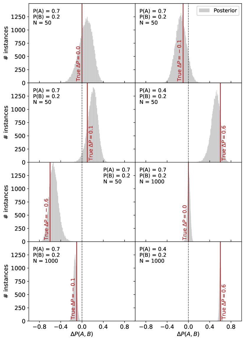
Figure 2. Histograms depicting the sampled $\Delta P(A,B)$ posterior distributions, showcasing results from eight simulations characterized by varying parameters of $\Delta P(A,B)$, $P(A=1)$, $P(B=1)$, and sample size $N$.

The posteriors cover the region around the true probability boost values set for the simulations. When the sample size is larger, the posterior is narrower.

3. Application to sentiment analysis

3.1. Data collection

Utilizing Twitter’s official API, we gathered 5,000 random tweets in Portuguese from the period of 12th to 20th March in 2022. To ensure we collected only tweets in portuguese, we set the attribute language to ’pt’. We exclueded retweets to keep only original content.

3.2. Text annotation

We formed one team comprised of three psychology undergraduate students as annotators. The team was assigned the task of classifying tweets based on emotional themes, drawing from a list of 30 categories influenced by a literature of emotions in portuguese (Cortiz et al., 2021). This list was further expanded to include the categories LOVE, AMUSEMENT, SCHADENFREUDE, and NEUTRAL.

Each annotator worked independently, with the freedom to label a tweet under multiple categories. The annotators were instructed to label all identified emotions in the same tweet. For a tweet to officially fall under a specific category, a consensus of at least two annotators was required. Tweets that only received a single annotator’s endorsement for a category were not categorized under that label. Tweets without any consensus were excluded from the dataset.

3.3. Results

Since annotators could assign multiple emotions to each tweet, we treated the identification of each emotion as an independent binary variable without any inter-variable constraints. Since we utilized 30 emotional categories in our study, there are $(30\cdot 29)/2=435$ pairs of variables for assessing dependence. To address the issue of multiple comparisons and mitigate the risk of false positives, we implemented the Bonferroni correction to the 2% significance level we would adopt in a single test. Consequently, we only considered pairs of variables with $p$-values below $4.6\cdot 10^{-5}$ as indicating statistically significant dependencies.

We generated posterior estimates using four parallel chains, each comprising 10,000 steps after the burn-in phase, resulting in 40,000 samples for every pair of emotions. Among the 435 pairs assessed, we identified 48 as dependent. Figure 3 illustrates the estimates for $P(A=1)$, $P(A=1|B=1)$, and $\Delta P(A,B)$ for the emotion permutation with the highest $|\Delta P(A,B)|$ in each pair.

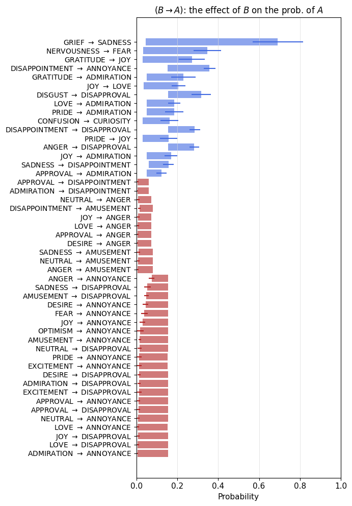
Figure 3. Probability boosts on sentiment $A$ detection given that another sentiment $B$ was already detected. Each bar starts at $P(A=1)$ and ends at $P(A=1|B=1)$. An error bar representing the standard deviation of $P(A=1|B=1)$ features at the end of each bar. The length of each bar represents $\Delta P(A,B)$, and the bar is blue when $\Delta P(A,B)>0$, and red otherwise. We only included emotion pairs with statistically significant dependence and the emotion permutation in each pair with the highest $|\Delta P|$.

Horizontal bar plot for each one of the 48 pairs of dependent emotions. The detection of grief boosts the probability for identifying sadness by almost 70 percent. The boosts on other emotions are smaller. Fear gets boosted by 30 percent if nervousness is already identified. Some emotions are almost excludent: if one is identified, the chance of detecting the other goes is compatible with zero.

The figure reveals several exciting relationships. In general, emotions that co-occur in a tweet tend to share the same polarity, be it positive, negative, or neutral, affirming the validity of such broad sentiment classifications. An interesting exception is the notable increase from 3% to 16% in the probability of detecting curiosity when confusion is already present. Nonetheless, this association between both emotions remains sensible.

Furthermore, as depicted in Fig. 3, there are instances where the presence of one emotion reduces the likelihood of finding the other in the same tweet. In most cases, this reduction drives the probability close to zero, implying that the emotions in these pairs are mutually exclusive. Notably, such exclusivity only occurs between emotions of differing polarities.

The negative boosts that do not drive the probabilities to zero reveal an intriguing finding: while not mutually exclusive, certain negative emotions tend to repel each other. In other words, they appear together less frequently than what chance would suggest. Notable examples include anger and annoyance, as well as disapproval and sadness. This observation might indicate distinct modes of adverse reaction.

Conversely, there are mixed-polarity pairs that, despite displaying repulsion, are not exclusive, meaning they occasionally co-occur. Examples of such pairs are disapproval and amusement, as well as annoyance and desire.

The significant boost that grief applies to sadness is striking: when grief is present, the probability of encountering sadness in a tweet surges from 4% to 69%. This substantial increase, which is not as pronounced in the opposite direction, signifies a hierarchical relationship between these two emotions. Grief is closely related to sadness, almost resembling a subclass of it. The Venn diagram in Fig. 4 visually represents this relationship, illustrating the number of tweets annotated with these two emotions. Out of the 11 tweets annotated with grief, a substantial eight were also annotated with sadness, an emotion detected in a significantly larger set containing 202 instances. The extensive overlap between the sets and their size disparities explain why detecting grief amplifies the likelihood of finding sadness by 65 percentage points (p.p.), whereas identifying sadness elevates the chance of detecting grief by only four p.p.

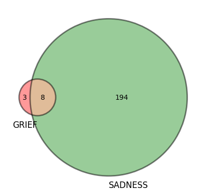
Figure 4. Venn diagram depicting the number of tweets annotated with grief and/or sadness.

194 tweets were annotated with sadness only, 3 with grief only and 8 with both. Since the total number of tweets containing grief is 11, the circle representing these tweets is almost completely inside the sadness circle.

Lastly, Fig. 5 presents an overview of the relationships between all emotions. We clustered the emotions using the boost $\Delta P$ with the highest modulus in each pair as a proximity measure. Specifically, we computed pairwise distances $D(A,B)$ between emotions using the formula:

(5) $$D(B,A)\equiv 0.01+\mathrm{max}(\Delta P)-\mathrm{max}[\Delta P(A,B),\Delta P(B,A)],$$

We employed this measure in the t-distributed stochastic neighbor embedding (t-SNE) (Hinton and Roweis, 2002) to project the emotions onto a 2D plane. In the equation above, $\mathrm{max}(\Delta P)$ represents the highest boost among all emotion pairs.

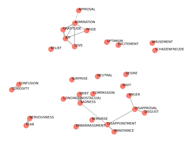
Figure 5. Graph of the relationships between emotions, represented as red nodes. Statistically significant positive boosts are represented by gray connections (graph edges). The width of the connections are proportional to the highest boost in each pair. The nodes’ positions were set with the tSNE technique.

A graph with 30 nodes and 16 edges. Positive emotions are clustered on the top, while negative emotions are clustered at the bottom.

In Fig. 5, emotions $A$ and $B$ were connected by a gray line whose width is proportional to $\mathrm{max}[\Delta P(A,B),\Delta P(B,A)]$ when $\Delta P$ was positive and statistically significant. Apart from the clear separation between positive emotions at the top and negative emotions at the bottom, we can identify four clusters of connected emotions and some disconnected ones.

4. Conclusions

In this paper, we have introduced a novel method for measuring the degree of association between categorical variables. This Bayesian approach is grounded in the formal definition of variable independence, $P(A|B)=P(A)$, and was implemented using Markov Chain Monte Carlo (MCMC) techniques. One of the key strengths of this method is that it provides a posterior distribution for our measure of association, offering detailed insights into the relationship between the two variables under study.

Another characteristic that sets this method apart is that it does not rely on prior knowledge of the total number of occurrences for any category, making it particularly well-suited for applications like sentiment analysis.

There are avenues for further exploration in this research. Firstly, our current prior assumes equal probability levels for detecting and non-detecting any given emotion among a set of 30 possibilities. Enhancing the method might involve adjusting this prior to reflect a higher probability of non-detection.

Additionally, future research could focus on finding an analytical derivation for the posterior of $\Delta P(A,B)$. If existent, the derivation could significantly enhance the efficiency of estimating the degree of association.

In our Twitter-based analysis, we observed consistent co-occurrences of specific emotions in tweets, providing empirical evidence for the predisposition of certain emotions to appear together. These emotional pairings can be interpreted through multiple theoretical lenses. According to the circumplex model (Russell and Barrett, 1999), the similar valence of frequently co-occurring emotions suggests that these combinations are not arbitrary but are likely to be shaped by inherent emotional dimensions. Take, for example, the pairing of ’grief’ and ’sadness,’ both of which have negative valence, thereby aligning closely within the circumplex framework.

The hierarchical models of emotion offer another insightful perspective (Shaver et al., 1987; Zelenski and Larsen, 2000). In our data, we noted pairings like ’nervousness’ and ’fear,’ where the former, a secondary emotion, commonly appears with the latter, a primary emotion. This finding underscores the hierarchical organization of these emotional states, supporting the notion that primary emotions serve as building blocks for secondary and tertiary emotions.

In addition to these theoretical implications, our findings suggest a practical dimension related to social communication. Emotions play pivotal roles in social bonding, communication, and even conflict (Keltner and Haidt, 1999). The frequent co-expression of emotions sharing similar valence may enrich Twitter’s emotional discourse, thereby contributing to more effective communication, message dissemination, and social interaction. This observation aligns with (Zelenski and Larsen, 2000), who found that positive emotions coalesce more readily than negative ones, a pattern also reflected in our data set.

Conclusively, our findings portray the co-occurring emotions in tweets as a complex interplay influenced by both dimensional and hierarchical frameworks, as well as by the social communicative needs of Twitter users. Future research is encouraged to delve into the repercussions of these emotional pairings on aspects like reader engagement, message virality, and the emotional well-being of the Twitter community.

References

- (1)
- Barnard (1945) G. A. Barnard. 1945. A New Test for 2 × 2 Tables. Nature 156 (1945), 177. https://doi.org/10.1038/156177a0
- Boschloo (1970) R. D. Boschloo. 1970. Raised conditional level of significance for the 2 × 2-table when testing the equality of two probabilities. Statistica Neerlandica 24, 1 (1970), 1–9. https://doi.org/10.1111/j.1467-9574.1970.tb00104.x arXiv:https://onlinelibrary.wiley.com/doi/pdf/10.1111/j.1467-9574.1970.tb00104.x
- Chmiel et al. (2011) Anna Chmiel, Julian Sienkiewicz, Mike Thelwall, Georgios Paltoglou, Kevan Buckley, Arvid Kappas, and Janusz A. Hołyst. 2011. Collective Emotions Online and Their Influence on Community Life. PLoS ONE 6 (7 2011), e22207. Issue 7. https://doi.org/10.1371/journal.pone.0022207
- Cortiz et al. (2021) Diogo Cortiz, Jefferson Silva, Newton Calegari, Ana Freitas, Ana Soares, Carolina Botelho, Gabriel Rêgo, Waldir Sampaio, and Paulo Boggio. 2021. A Weakly Supervised Dataset of Fine-Grained Emotions in Portuguese. In Anais do XIII Simpósio Brasileiro de Tecnologia da Informação e da Linguagem Humana (Evento Online). SBC, Porto Alegre, RS, Brasil, 73–81. https://doi.org/10.5753/stil.2021.17786
- Fisher (1922) R. A. Fisher. 1922. On the Interpretation of from Contingency Tables, and the Calculation of P. Journal of the Royal Statistical Society 85, 1 (1922), 87–94. http://www.jstor.org/stable/2340521
- Goodman and Kruskal (1954) Leo A. Goodman and William H. Kruskal. 1954. Measures of Association for Cross Classifications. J. Amer. Statist. Assoc. 49, 268 (1954), 732–764. http://www.jstor.org/stable/2281536
- Hinton and Roweis (2002) Geoffrey E Hinton and Sam Roweis. 2002. Stochastic Neighbor Embedding. In Advances in Neural Information Processing Systems, S. Becker, S. Thrun, and K. Obermayer (Eds.), Vol. 15. MIT Press. https://proceedings.neurips.cc/paper_files/paper/2002/file/6150ccc6069bea6b5716254057a194ef-Paper.pdf
- Keltner and Haidt (1999) Dacher Keltner and Jonathan Haidt. 1999. Social Functions of Emotions at Four Levels of Analysis. Cognition and Emotion 13, 5 (1999), 505–521. https://doi.org/10.1080/026999399379168 arXiv:https://doi.org/10.1080/026999399379168
- Olsson (1979) U. Olsson. 1979. Maximum likelihood estimation of the polychoric correlation coefficient. Psychometrika 44 (1979), 443–460. https://link.springer.com/article/10.1007/BF02296207
- Pearl et al. (2016) Judea Pearl, Madelyn Glymour, and Nicholas P. Jewell. 2016. Causal inference in statistics: a primer (1st. ed.). Wiley, West Sussex, UK.
- Press et al. (2007) William H. Press, Saul A. Teukolsky, and William T. Vetterling. 2007. Numerical Recipes: The Art of Scientific Computing (3rd. ed.). Cambridge University Press, Cambridge, England.
- Russell and Barrett (1999) James Russell and Lisa Barrett. 1999. Core affect, prototypical emotional episodes, and other things called emotion: Dissecting the elephant. Journal of personality and social psychology 76 (06 1999), 805–19. https://doi.org/10.1037//0022-3514.76.5.805
- Russell (1980) James A. Russell. 1980. A circumplex model of affect. Journal of Personality and Social Psychology 39 (12 1980), 1161–1178. Issue 6. https://doi.org/10.1037/h0077714
- Salvatier et al. (2016) John Salvatier, Thomas V. Wiecki, and Christopher Fonnesbeck. 2016. Probabilistic programming in Python using PyMC3. PeerJ Computer Science 2 (2016), e55. https://doi.org/10.7717/peerj-cs.55
- Schwarz (2022) Norbert Schwarz. 2022. Situated cognition and the wisdom of feeling: Cognitive tuning. In The wisdom in feeling, Lisa Feldman Barrett (Ed.). Guilford, New York, 144–166.
- Shaver et al. (1987) Phillip Shaver, Judith Schwartz, Donald Kirson, and Cary O’Connor. 1987. Emotion knowledge: Further exploration of a prototype approach. Journal of Personality and Social Psychology 52 (1987), 1061–1086. Issue 6. https://doi.org/10.1037/0022-3514.52.6.1061
- Stieglitz and Dang-Xuan (2013) Stefan Stieglitz and Linh Dang-Xuan. 2013. Emotions and Information Diffusion in Social Media—Sentiment of Microblogs and Sharing Behavior. Journal of Management Information Systems 29 (4 2013), 217–248. Issue 4. https://doi.org/10.2753/MIS0742-1222290408
- Szumilas (2015) Magnalena Szumilas. 2015. Explaining odds ratios. J. Can. Acad. Child Adolesc. Psychiatry 24, 1 (2015), 58. https://www.ncbi.nlm.nih.gov/pmc/articles/PMC2938757/
- Zelenski and Larsen (2000) John M. Zelenski and Randy J. Larsen. 2000. The Distribution of Basic Emotions in Everyday Life: A State and Trait Perspective from Experience Sampling Data. Journal of Research in Personality 34, 2 (2000), 178–197. https://doi.org/10.1006/jrpe.1999.2275