The Frank-Wolfe algorithm: a short introduction

Abstract

In this paper we provide an introduction to the Frank-Wolfe algorithm, a method for smooth convex optimization in the presence of (relatively) complicated constraints. We will present the algorithm, introduce key concepts, and establish important baseline results, such as e.g., primal and dual convergence. We will also discuss some of its properties, present a new adaptive step-size strategy as well as applications.

(Article for the Jahresbericht der Deutschen Mathematiker Vereinigung)

1 Introduction

Throughout this paper we will be concerned with constrained optimization problems of the form

$$\min_{x\in P}f(x),$$ (Opt)

where $P\subseteq{\mathbb{R}}^{n}$ is some convex feasible region capturing the constraints, e.g., a polyhedron arising from a system of linear inequalities or a spectrahedron, and $f$ is the objective function satisfying some regularity property, e.g., smoothness and convexity. We also need to specify what access methods we have, both, to the function and the feasible region. A common setup is black box first-order access for $f$, allowing (only) the computation of gradients $\nabla f(x)$ for a given point $x$ as well as the function value $f(x)$. For the access to the feasible region $P$, which we will assume to be compact in the following, there are several common models; we simplify the exposition here for the sake of brevity:

1. Projection. Access to the projection operator $\Pi_{P}$ of $P$ that, for a given point $x\in\mathbb{R}^{n}$ returns $\Pi_{P}(x)\doteq\operatorname{argmin}_{y\in P}\|x-y\|$, for some norm $\|.\|$ (or more generally Bregman divergences).

2. Barrier function. Access to a barrier function of the feasible region $P$ that increases in value to infinity when approaching the boundary of $P$. A typical example is, the barrier function $-\sum_{i}\log(b_{i}-A_{i}x)$ for a linear inequality system $P\doteq\{x\mid Ax\leq b\}$.

3. Linear Minimization. Access to a Linear Minimization Oracle (LMO) that, given a linear objective $c\in\mathbb{R}^{n}$, returns $y\in\operatorname{argmin}_{x\in P}\mathinner{{}\langle c,x\rangle}$.

Specialized approaches for specific cases, e.g., the simplex method (Dantzig,, 1981; 1983) in the case of linear objectives which uses an explicit description of the feasible region also exist but here we concentrate on the aforementioned black box model. There are also proximal methods, which can be considered generalizations of projection-based methods and which we will not explicitly consider for the sake of brevity; see e.g., Nemirovski and Yudin, (1983); Nesterov, (2004; 2018); Nocedal and Wright, (2006) for a discussion.

Traditionally, problems of the form (Opt) are solved by variants of projection-based methods. In particular first-order methods, such as variants of projected gradient descent are often chosen in large-scale contexts as they are comparatively cheap. For some feasible region $P$ with projector $\Pi_{P}$ (e.g., $\Pi_{P}(x)\doteq\operatorname{argmin}_{y\in P}\|x-y\|$) and smooth objective function $f$, projected gradient descent (PGD) updates typically take the form:

$$x_{t+\nicefrac{{1}}{{2}}} \leftarrow x_{t}-\gamma_{t}\nabla f(x_{t})$$ (PGD)

$$x_{t+1} \leftarrow\Pi_{P}(x_{t+\nicefrac{{1}}{{2}}}),$$

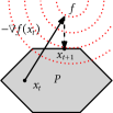
where $\gamma_{t}$ is some step-size, e.g., $\gamma_{t}=1/L$ if $f$ is $L$-smooth (see Definition 2.1) and convex. In essence, a descent step is taken without considering the constraints, and then it is projected back into the feasible region (see Figure 3). Projection-based first-order methods have been extensively studied, with comprehensive overviews available in, e.g., Nesterov, (2018); Nocedal and Wright, (2006). Optimal methods and rates are known for most scenarios. Efficient execution of the projection operation is possible for simple constraints, such as box constraints or highly structured feasible regions, e.g., as discussed in Moondra et al., (2021); Gupta et al., (2016) for submodular base polytopes. However, when the feasible region grows in complexity, the projection operation can become the limiting factor. It often demands the solution of an auxiliary optimization problem—known as the projection problem—over the same feasible region for every descent step. This complexity renders the use of projection-based methods for many significant constrained problems quite challenging; in some cases relaxed projections which essentially compute separating hyperplanes can be used though.

Interior point methods (IPM) offer an alternative approach, see e.g., Boyd et al., (2004); Potra and Wright, (2000). To illustrate this approach, consider the goal of minimizing a linear function $c$ over a polytope defined as $P\doteq\{x\mid Ax\leq b\}$. The typical updates in a path-following IPM resemble:

$$x_{\mu} \leftarrow\operatorname{argmin}_{x}\mathinner{{}\langle c,x\rangle}+\mu\sum\log(b_{i}-A_{i}x),$$ (IPM)

where the value of $\mu\rightarrow 0$ according to some strategy for $\mu$. Often, these steps are only approximately solved. IPMs, while potent with appealing theoretical guarantees, usually necessitate a barrier function that encapsulates the feasible region’s description. In numerous critical scenarios, a concise feasible region description is either unknown or proven to be non-existent. For instance, the matching polytope does not admit small linear programs, neither exact ones (Rothvoss,, 2017) nor approximate ones (Braun and Pokutta, 2015a, ; Braun and Pokutta, 2015b, ; Sinha,, 2018). Additionally, achieving sufficient accuracy in the IPM step updates often requires second-order information, which can sometimes restrict its applicability.

Upon closely examining the two methods mentioned earlier, it is clear that both essentially transform the constrained problem (Opt) into an unconstrained one. They then either correct updates that violate constraints (as in PGD) or penalize nearing constraint violations (as in IPM). Yet, another category of techniques exists, termed projection-free methods, which focus directly on constrained optimization. Unlike their counterparts, these methods sidestep the need for costly projections or penalty strategies and maintain feasibility throughout the process. The most notable variants in this category are the Frank-Wolfe (FW) methods—going back to Frank and Wolfe, (1956)—which will be the focus of this article and which are also known as conditional gradient (CG) methods (Levitin and Polyak,, 1966).

Historically, methods like the Frank-Wolfe algorithm garnered limited attention because of certain drawbacks, notably sub-optimal convergence rates. However, there was a notable resurgence in interest around 2013. This revival is largely attributed to shifting requirements and their other, now suddenly relevant properties. Notably, these methods are well suited to handle complicated constraints and possess a low iteration complexity. This makes them very effective in the context of large-scale machine learning problems (see, e.g., (Lacoste-Julien et al.,, 2013; Jaggi,, 2013; Négiar et al.,, 2020; Dahik,, 2021; Jing et al.,, 2023)), image processing (see, e.g., (Joulin et al.,, 2014; Tang et al.,, 2014)), quantum physics (see, e.g., (Gilbert,, 1966; Designolle et al., 2023a, )), submodular function maximization (see, e.g., (Feldman et al.,, 2011; Vondrák,, 2008; Badanidiyuru and Vondrák,, 2014; Mirzasoleiman et al.,, 2016; Hassani et al.,, 2017; Mokhtari et al., 2018a, ; Anari et al.,, 2019; 2021; Mokhtari et al., 2018b, ; Bach,, 2019)), online learning (see, e.g., (Hazan and Kale,, 2012; Zhang et al.,, 2017; Chen et al.,, 2018; Garber and Kretzu,, 2021; Kerdreux et al.,, 2021; Zhang et al.,, 2023)) and many more (see, e.g., (Bolte et al.,, 2007; Clarkson,, 2010; Pierucci et al.,, 2014; Harchaoui et al.,, 2015; Wang et al.,, 2016; Cheung and Li,, 2018; Ravi et al.,, 2019; Hazan and Minasyan,, 2020; Dvurechensky et al.,, 2020; Carderera and Pokutta,, 2020; Macdonald et al.,, 2022; Carderera et al.,, 2021; Garber and Wolf,, 2021; Bomze et al.,, 2021; Wäldchen et al.,, 2022; Chen and Sun,, 2023; de Oliveira,, 2023; Designolle et al., 2023a, ; Designolle et al., 2023b, ; Lacoste-Julien,, 2016)). Moreover, there has been a proliferation of modifications to these methods, addressing many of their historical limitations (see, e.g., (Freund et al.,, 2017; Lacoste-Julien and Jaggi,, 2015; Garber and Hazan,, 2015; 2016; Lan et al.,, 2017; Braun et al.,, 2017; Braun et al., 2019b, ; Braun et al., 2019a, ; Combettes and Pokutta,, 2020; Tsuji et al.,, 2022)) and there is an intricate connection between Frank-Wolfe methods and subgradients methods (Bach,, 2015); see Braun et al., 2022a for a comprehensive exposition.

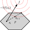
Rather than relying on potentially expensive projection operations (see Figure 3), Frank-Wolfe methods use a so-called Linear Minimization Oracle (LMO). This subroutine only involves optimizing a linear function over the feasible region, often proving more cost-effective than traditional projections; see Combettes and Pokutta, (2021) for an in-depth comparison. The nuclear norm ball, along with matrix completion, is a prime example highlighting the difference in complexity. The core updates in Frank-Wolfe methods often rely on the following fundamental update:

$$v_{t} \leftarrow\operatorname{argmin}_{v\in P}\mathinner{{}\langle\nabla f(x_{t}),v\rangle}$$ (FW)

$$x_{t+1} \leftarrow(1-\gamma_{t})x_{t}+\gamma_{t}v_{t},$$

where any solution to the $\operatorname{argmin}$ is suitable and $\gamma_{t}$ follows some step-size strategy, e.g., $\gamma_{t}=\frac{2}{2+t}$. Essentially, the LMO identifies an alternate direction for descent. Subsequently, convex combinations of points are constructed within the feasible region to maintain feasibility. Viewed through the lens of complexity theory, the Frank-Wolfe methods reduce the optimization of a convex function $f$ over $P$ into the repeated optimization of evolving linear functions over $P$. A schematic of the most basic variant of the Frank-Wolfe algorithm is shown in Figure 3.

For a more comprehensive exposition complementing this introductory article the interested reader is referred to Braun et al., 2022a ; the notation has been deliberately chosen to be matching whenever possible.

Figure 1: Projection-based methods: may require (potentially expensive) projection back into $P$ to ensure feasibility.

Figure 2: Projection-free methods: ensure feasibility by forming convex combinations only.
 

1   $x_{0}\in P$

2   for $t=0$ to $T-1$ do

3      $v_{t}\leftarrow\operatorname{argmin}\limits_{v\in P}\langle{\nabla f(x_{t})},v\rangle$

4      $x_{t+1}\leftarrow(1-\gamma_{t})x_{t}+\gamma_{t}v_{t}$

5   end for

Algorithm 1 FW algorithm

Figure 3: New iterates are formed by convex combination with an extreme point approximating the gradient, ensuring feasibility.

Outline

We start with some basic notions and notations in Section 2 and then present the original Frank-Wolfe algorithm along with some motivation in Section 3. We then proceed in Section 4 with establishing basic properties, such as e.g., convergence and also provide matching lower bounds. While this is primarily an overview article, we do provide a new adaptive step-size strategy in Section 4.5, which is also available in the FrankWolfe.jl julia package. In Section 5 we then consider applications of the Frank-Wolfe algorithm and also discuss computational aspects in Section 6.

2 Preliminaries

In the following $\|\cdot\|$ will denote the $2$-norm if not stated otherwise. Note however that in general other norms are possible and have been used in the context of Frank-Wolfe algorithms. Moreover, for simplicity we assume that $f$ is differentiable, which is a standard assumption in the context of Frank-Wolfe algorithms although non-smooth variants are known (see, e.g., Braun et al., 2022a for details).

For our analysis we will heavily rely on the following key concepts:

Definition 2.1 (Convexity and Strong Convexity).

Let $f\colon P\rightarrow{\mathbb{R}}$ be a differentiable function. Then $f$ is convex if

$$f(y)-f(x)\geq\mathinner{{}\langle\nabla f(x),y-x\rangle}\quad\text{for all }x,y\in P.$$ (2.1)

Moreover, $f$ is $\mu$-strongly convex if

$$f(y)-f(x)\geq\mathinner{{}\langle\nabla f(x),y-x\rangle}+\frac{\mu}{2}\|y-x\|^{2}\quad\text{for all }x,y\in P.$$ (2.2)

Definition 2.2 (Smoothness).

Let $f\colon P\to{\mathbb{R}}$ be a differentiable function. Then $f$ is $L$-smooth if

$$f(y)-f(x)\leq\mathinner{{}\langle\nabla f(x),y-x\rangle}+\frac{L}{2}\|y-x\|^{2}\quad\text{for all }x,y\in P.$$ (2.3)

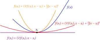
The smoothness and (strong) convexity inequalities from above allow us to obtain upper and lower bounds on the function $f$. Convexity and strong convexity provide respectively linear and quadratic lower bounds on the function $f$ at a given point $x$ while smoothness provides a quadratic upper bound as shown in Figure 5.

For completeness we note that, both, $L$-smoothness and $\mu$-strong convexity can also be expressed without relying on function values of $f$ only using gradients $\nabla f$. This is in particular useful in the context of an adaptive step-size strategy that we will discuss in Section 4.5 as it significantly improves numerical stability of the estimates.

Remark 2.3 (Smoothness and Strong Convexity via Gradients).

Let $f\colon P\rightarrow{\mathbb{R}}$ be a differentiable function. Then $f$ is $L$-smooth if

$$\mathinner{{}\langle\nabla f(y)-\nabla f(x),y-x\rangle}\leq L\|y-x\|^{2}\quad\text{for all }x,y\in P,$$ (2.4)

and similarly $f$ is $\mu$-strongly convex if

$$\mathinner{{}\langle\nabla f(y)-\nabla f(x),y-x\rangle}\geq\mu\|y-x\|^{2}\quad\text{for all }x,y\in P.$$ (2.5)

There is also the closely related and seemingly stronger property of $L$-Lipschitz continuous gradient $\nabla f$, however in the case that $P$ is full-dimensional and $f$ is convex it is known to be equivalent to $L$-smoothness (see Nesterov, (2018, Theorem 2.1.5) for the unbounded case, i.e., where $P={\mathbb{R}}^{n}$ and Braun et al., 2022a (, Lemma 1.7) for $P$ being arbitrary convex domain). In particular, for twice differentiable convex functions $f$, we can also capture smoothness and strong convexity in terms of the Hessian via $\|\nabla^{2}f\|\leq L$ and via the largest eigenvalue of $\nabla^{2}f$ being upper bounded by $L\geq 0$ and the smallest eigenvalue being lower bounded by $\mu\geq 0$, respectively; the first inequality is useful for numerical estimation of $L$.

Figure 4: (Strong) convexity and smoothness provide linear and quadratic approximations to $f$. Orange: quadratic upper bound via smoothness, Red: quadratic lower bound via strong convexity, Magenta: linear lower bound via convexity, Blue: function $f$.

Figure 5: The Frank–Wolfe step: To minimize a convex function $f$ over a polytope $P$, a linear approximation of $f$ is constructed at $x_{t}$ as $f(x_{t})+\mathinner{{}\langle\nabla f(x_{t}),x-x_{t}\rangle}$. The Frank–Wolfe vertex $v_{t}$ minimizes this approximation. The step transitions from $x_{t}$ to $x_{t+1}$ by moving towards $v_{t}$ as determined by a step-size rule. Contour lines of $f$ in red and linear approximation blue.

In the following the domain $P$ will be a compact convex set and we assume that we have access to a so-called Linear Minimization Oracle (LMO) for $P$, which upon being provided with a linear objective function $c$ returns a minimizer $v=\operatorname{argmin}_{x\in P}\mathinner{{}\langle c,x\rangle}$ as formalized in Algorithm 2. Note that $v$ is not necessarily unique and without loss of generality we assume that $v$ is an extreme point of $P$; these extreme points are also often called atoms in the context of Frank-Wolfe algorithms. For the compact convex set $P$ the diameter $D$ of $P$ is defined as $D\doteq\max_{x,y\in P}\|x-y\|$.

Regarding the function $f$ we assume that we have access to gradients and function evaluations which is formalized as First-Order Oracle (denoted as FOO), which given a point $x\in P$, returns the function value $f(x)$ and gradient $\nabla f(x)$ at $x$; see Algorithm 3. In the following we let $x^{*}$ be one of the optimal solutions to $\min_{x\in P}f(x)$ and define further $f^{*}\doteq f(x^{*})$. Moreover, if not stated otherwise we consider $f\colon P\rightarrow{\mathbb{R}}$.

0   Linear objective $c$

0   $v\in\operatorname{argmin}_{x\in P}\mathinner{{}\langle c,x\rangle}$

Algorithm 2 Linear Minimization Oracle over $P$ (LMO)

0   Point $x\in P$

0   $\nabla f(x)$ and $f(x)$ $\operatorname{argmin}_{x\in P}\mathinner{{}\langle c,x\rangle}$

Algorithm 3 First-Order Oracle for $f$ (FOO) over $P$ (LMO)

Figure 6: Access to function $f$ and feasible region $P$ is via two functions that we assume to have (oracle) access to.

3 The Frank-Wolfe algorithm

We will now introduce the original variant of the Frank-Wolfe (FW) algorithm due to Frank and Wolfe, (1956), which is often also referred to as Conditional Gradients (Levitin and Polyak,, 1966). Although many advanced variants with enhanced properties and improved convergence in specific problem configurations exist today, we will focus on the original version for clarity and to underscore the fundamental concepts.

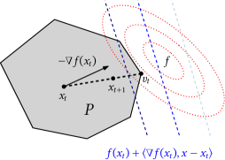
Suppose we are interested in minimizing a smooth and convex function $f$ over some compact convex feasible set $P$. A natural strategy would be to follow the negative of the gradient $\nabla f(x)$ at a given point $x$. However, how far can we go into that direction before we hit the boundary of the feasible region? Moreover, even if we would know how far we can go, i.e., we would potentially truncate steps to not leave the feasible region, even then the resulting algorithm might not be converging to an optimal solution. In fact, the arguably most well-known strategy, the projected gradient descent method does not simply stop at the boundary but follows the negative of the gradient according to some step-size, disregarding the constraints, and then projects back onto the feasible region. This last step can be very costly: if we do not have an efficient formulation or algorithm for the projection problem, solving this projection problem can be a (relatively expensive) optimization problem in itself. In contrast, the basic idea of the Frank-Wolfe algorithm is to not follow the negative of the gradient but to follow an alternative direction of descent, which is well-enough aligned with the negative of the gradient, ensures enough primal progress, and for which we can easily ensure feasibility by means of computing convex combinations. This is done via the aforementioned Linear Minimization Oracle, with which we can optimize the negative of the gradient over the feasible region $P$ and then take the obtained vertex to form an alternative direction of descent. The overall process is outlined in Figure 5 and in Algorithm 4 we provide the Frank-Wolfe algorithm, which only requires access to (Opt) via the LMO (see Algorithm 2) to access the feasible region and via the FOO (see Algorithm 3) to access the function.

0   Initial atom $x_{0}\in P$, smooth and convex objective function $f$

0   Iterates $x_{1},\dotsc\in P$

1   for $t=0$ to … do

2       $v_{t}\leftarrow\operatorname{argmin}_{v\in P}\mathinner{{}\langle\nabla f(x_{t}),v\rangle}$

3       $\gamma_{t}\leftarrow\frac{2}{2+t}$

4      $x_{t+1}\leftarrow(1-\gamma_{t})x_{t}+\gamma_{t}v_{t}$

5   end for

Algorithm 4 Frank–Wolfe algorithm

As can be seen, assuming access to the two oracles, the actual implementation is very straight-forward: a simple computation of a convex combination, which ensures that we do not leave the feasible region. We made the deliberate choice in Line 3 of Algorithm 4 to use the most basic step-size strategy $\gamma_{t}=\frac{2}{2+t}$, the so-called open loop or agnostic step-size, as this makes the algorithm parameter-independent, i.e., not requiring any function parameters or parameter estimations. In the worst-case, this step-size is not dominated by more elaborate strategies (such as, e.g., line search or short steps), however in many important special cases there are better choices. As this is crucial we will discuss this a little more in-depth in Section 4.5 and will also provide a new variant of an adaptive step-size strategy.

Another important property is that the algorithm is affine invariant, i.e., problem rescaling etc. does not affect the algorithm’s performance, compared to most other methods including PGD (notable exceptions exist, e.g., Newton’s method). This makes the algorithm also very robust (especially with the open loop step-sizes) often offering superior numerical stability.

Finally, we would like to mention that at iteration $t$ the iterate $x_{t}$ is a convex combination of at most $t+1$ extreme points (or atoms) of $P$. This will allow us later to obtain sparsity vs. approximation trade-offs in Section 4.1.

4 Properties

We will now establish key properties of Algorithm 4. We start with convergence properties and will then establish matching lower bounds as well as other properties.

4.1 Convergence

We will now prove the convergence of the Frank-Wolfe algorithm (Algorithm 4). Convergence proofs for these methods typically use two key ingredients, which we will introduce in the following.

Lemma 4.1 (Primal gap, Dual gap, and Frank-Wolfe gap).

Let $f$ be a convex function and $P$ a compact convex set and consider (Opt). For all $x\in P$ it holds:

$$\underbrace{f(x)-f(x^{*})}_{\text{primal gap at $x$}}\leq\underbrace{\mathinner{{}\langle\nabla f(x),x-x^{*}\rangle}}_{\text{dual gap at $x$}}\leq\underbrace{\max_{v\in P}\mathinner{{}\langle\nabla f(x),x-v\rangle}}_{\text{Frank-Wolfe gap at $x$}}.$$ (FW-gap)

Proof.

The first inequality follows from convexity and the second inequality follows from maximality. ∎

The Frank-Wolfe gap plays a crucial role in the theory of Frank-Wolfe methods as it provides an easily computable optimality certificate and suboptimality gap measure. An extreme point $v\in\operatorname{argmax}_{z\in P}\mathinner{{}\langle\nabla f(x),x-z\rangle}$, is typically referred to as Frank-Wolfe vertex for $\nabla f(x)$. The Frank-Wolfe gap also naturally appear in the first-order optimality condition for (Opt), which states that $x^{*}\in P$ is optimal for (Opt) if and only if the Frank-Wolfe gap at $x^{*}$ is equal to $0$. Note that in the constrained case it does not necessarily hold that $\nabla f(x^{*})=0$.

Lemma 4.2 (First-order Optimality Condition).

Let $x^{*}\in P$. Then $x^{*}$ is an optimal solution to (Opt) if and only if

$$\mathinner{{}\langle\nabla f(x^{*}),x^{*}-v\rangle}\leq 0$$

for all $v\in P$. In particular, we have that the Frank-Wolfe gap $\max_{v\in P}\mathinner{{}\langle\nabla f(x^{*}),x^{*}-v\rangle}=0$.

The second property that is crucial is smoothness as it allows us to lower bound the primal progress we can derive from a step of the Frank-Wolfe algorithm.

Lemma 4.3 (Primal progress from smoothness).

Let $f$ be an $L$-smooth function and let $x_{t+1}=(1-\gamma_{t})x_{t}+\gamma_{t}v_{t}$ with $x_{t},v_{t}\in P$. Then we have

$$f(x_{t})-f(x_{t+1})\geq\gamma_{t}\mathinner{{}\langle\nabla f(x_{t}),x_{t}-v_{t}\rangle}-\gamma_{t}^{2}\frac{L}{2}\|x_{t}-v_{t}\|^{2}.$$ (4.1)

Proof.

The statement follows directly from the smoothness inequality (2.3)

$$f(y)-f(x)\leq\mathinner{{}\langle\nabla f(x),y-x\rangle}+\frac{L}{2}\|y-x\|^{2},$$

choosing $x\leftarrow x_{t}$ and $y\leftarrow x_{t+1}$, plugging in the definition of $x_{t+1}$, and rearranging. This gives the desired inequality

$$f(x_{t})-f(x_{t+1})\geq\gamma_{t}\mathinner{{}\langle\nabla f(x_{t}),x_{t}-v_{t}\rangle}-\gamma_{t}^{2}\frac{L}{2}\|x_{t}-v_{t}\|^{2}.$$

∎

With these two key ingredients (Lemma 4.1 and Lemma 4.3) we can now establish the basic convergence rate of the Frank-Wolfe algorithm:

Theorem 4.4 (Primal convergence of the Frank-Wolfe algorithm).

Let $f$ be an $L$-smooth convex function and let $P$ be a compact convex set of diameter $D$. Consider the iterates of Algorithm 4. Then the following holds:

$$f(x_{t})-f(x^{*})\leq\frac{2LD^{2}}{t+2},$$

and hence for any accuracy $\varepsilon>0$ we have $f(x_{t})-f(x^{*})\leq\varepsilon$ for all $t\geq\frac{2LD^{2}}{\varepsilon}$.

Proof.

The convergence proof of the Frank-Wolfe algorithm follows an approach that is quite representative for convergence results in that area. The proof follows the template outlined in Braun et al., 2022a and mimics closely the proof in Jaggi, (2013).

Our starting point is the inequality from Lemma 4.3

$$f(x_{t})-f(x_{t+1}) \geq\gamma_{t}\mathinner{{}\langle\nabla f(x_{t}),x_{t}-v_{t}\rangle}-\gamma_{t}^{2}\frac{L}{2}\|x_{t}-v_{t}\|^{2}$$

$$\geq\gamma_{t}(f(x_{t})-f(x^{*}))-\gamma_{t}^{2}\frac{L}{2}\|x_{t}-v_{t}\|^{2}.$$ (Lemma 4.1)

Subtracting $f(x^{*})$ on both sides, bounding $\|x_{t}-v_{t}\|\leq D$, and rearranging leads to

$$f(x_{t+1})-f(x^{*})\leq(1-\gamma_{t})(f(x_{t})-f(x^{*}))+\gamma_{t}^{2}\frac{LD^{2}}{2}.$$ (4.2)

This contraction relates the primal gap at $x_{t+1}$ with the primal gap at $x_{t}$. We conclude the proof by induction. First observe that for $t=0$ by (4.2) it follows

$$f(x_{1})-f(x^{*})\leq\frac{LD^{2}}{2}\leq\frac{2LD^{2}}{2}.$$

Now consider $t\geq 1$. We have

$$f(x_{t+1})-f(x^{*}) \leq(1-\gamma_{t})(f(x_{t})-f(x^{*}))+\gamma_{t}^{2}\frac{LD^{2}}{2}$$

$$\leq\frac{t}{2+t}(f(x_{t})-f(x^{*}))+\frac{4}{(2+t)^{2}}\frac{LD^{2}}{2} \gamma_{t}$$ (definition of )

$$\leq\frac{t}{2+t}\frac{2LD^{2}}{2+t}+\frac{4}{(2+t)^{2}}\frac{LD^{2}}{2}$$ (induction hypothesis)

$$=\frac{2LD^{2}}{t+3}\left(\frac{(3+t)(1+t)}{(2+t)^{2}}\right)\leq\frac{2LD^{2}}{t+3}, (3+t)(1+t)\leq(2+t)^{2}$$ ()

which completes the proof. ∎

The theorem above provides a convergence guarantee for the primal gap. However, it relies on knowledge of the diameter $D$ and Lipschitz constant $L$ for estimating the number of required iterations to reach a certain target accuracy $\varepsilon$. We can also consider the Frank-Wolfe gap $\max_{v_{t}\in P}\mathinner{{}\langle\nabla f(x_{t}),x_{t}-v_{t}\rangle}$, which upper bounds the primal gap $f(x_{t})-f(x^{*})$ via Lemma 4.1. While this gap is not monotonously decreasing (similar to the primal gap in the case of the open loop step-size) it is readily available in each iteration and hence can be used as a stopping criterion, i.e., we stop the algorithm when $\max_{v_{\tau}\in P}\mathinner{{}\langle\nabla f(x_{\tau}),x_{\tau}-v_{\tau}\rangle}\leq\varepsilon$, not requiring a priori knowledge about $D$ and $L$. For the running minimum we can establish a convergence rate similar to that in Theorem 4.4; see Jaggi, (2013), see also Braun et al., 2022a (, Theorem 2.2 and Remark 2.3).

Theorem 4.5 (Frank-Wolfe gap convergence of the Frank-Wolfe algorithm).

Let $f$ be an $L$-smooth convex function and let $P$ be a compact convex set of diameter $D$. Consider the iterates of Algorithm 4. Then the running minimum of the Frank–Wolfe gaps up to iteration $t$ satisfies:

$$\min_{0\leq\tau\leq t}\max_{v_{\tau}\in P}\mathinner{{}\langle\nabla f(x_{\tau}),x_{\tau}-v_{\tau}\rangle}\leq\frac{6.75\,LD^{2}}{t+2}$$

Another important property of the Frank-Wolfe algorithm is that it maintains convex combinations of extreme points and in each iteration at most one new extreme point is added. This leads to a natural accuracy vs. sparsity trade-off, where sparsity broadly refers to having convex combinations with a small number of vertices. This property is very useful and has been exploited repeatedly to prove mathematical results via applying the convergence guarantee of the Frank-Wolfe algorithm; we will see such an example further below in Section 5.1

4.2 A matching lower bound

In this section we will now provide a matching lower bound example due to Lan, (2013); Jaggi, (2013) that will require $\Omega(LD^{2}/\varepsilon)$ LMO calls to achieve an accuracy of $\varepsilon$ for an $L$-smooth function $f$ and a feasible region of diameter $D$. This lower bound holds for any algorithm that accesses the feasible region solely through an LMO and shows that in general the convergence rate of the Frank-Wolfe algorithm in Theorem 4.4 cannot be improved. We consider

$$\min_{x\in\operatorname{conv}{\{e_{1},\dots,e_{n}\}}}\|x\|^{2},$$

i.e., we minimize the standard quadratic $f(x)=\|x\|^{2}$ over the probability simplex $P\doteq\operatorname{conv}{\{e_{1},\dots,e_{n}\}}$, where the $e_{i}$ denote the standard basis vectors in $\mathbb{R}^{n}$, i.e., we have $L=2$ and $D=\sqrt{2}$ and any other combination of values for $L$ and $D$ can be obtained via rescaling. As $f$ is strongly convex it has a unique optimal solution, which is easily seen to be $x^{*}=(\frac{1}{n},\dots,\frac{1}{n})$ with optimal objective function value $f(x^{*})=\frac{1}{n}$. Note that the optimal solution lies in the relative interior of $P$, one of the earliest cases in which improved convergence rates for Frank-Wolfe methods have been obtained (GuéLat and Marcotte,, 1986).

If we now run the Frank-Wolfe algorithm from any extreme point $x_{0}$ of $P$, then after $t<n$ iterations, we have made $t$ LMO calls, and hence have picked up at most $t+1$ of the $n$ standard basis vectors. This is the only information available to us about the feasible region and by convexity the only feasible points the algorithm can create are convex combinations $x_{t}$ of these picked up extreme points. Thus it holds

$$f(x_{t})\geq\min_{\begin{subarray}{c}x\in\operatorname{conv}{\mathcal{S}}\\ \mathcal{S}\subseteq\{e_{1},\dots,e_{n}\}\\ |\mathcal{S}|\leq t+1\end{subarray}}f(x)=\frac{1}{t+1}.$$

Therefore the primal gap after $t$ iterations satisfies $f(x_{t})-f(x^{*})\geq 1/(t+1)-1/n$ and thus with the choice $n\gg 1/\varepsilon$ we need $\Omega(1/\varepsilon)$ LMO calls to guarantee a primal gap of at most $\varepsilon$. Finally, observe that this example also provides an inherent sparsity vs. optimality tradeoff: if we aim for a solution with sparsity $t$, then the primal gap can be as large as $f(x_{t})-f(x^{*})\geq 1/(t+1)-1/n$.

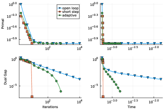
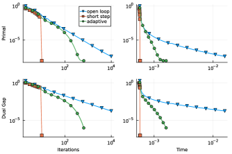
However, several remarks are in order to put this example into perspective. First of all, the lower bound example only holds up to the dimension $n$ of the problem and that is for good reason. Once we pass the dimension threshold, the lower bound is not instructive any more and other step-size strategies might achieve linear rates for $t\geq n$, and in particular if the step-size is the short step rule (see also Section 4.5) with exact smoothness $L$ we are optimal after exactly $t=n-1$ iterations; see Figures 8 and 8 for computational examples. Moreover, here we considered convergence rates independent of additional problem parameters. Introducing such parameters might provide more granular convergence rates under mild assumptions as shown, e.g., in Garber, (2020). There is also a different lower bound of $\Omega(1/\varepsilon)$ by Wolfe, (1970) (see also Braun et al., 2022a (, Theorem 2.8)) that is based around the so-called zigzagging phenomenon of the Frank-Wolfe algorithm and that holds beyond the dimension threshold. However, it only holds for step-size strategies—grossly simplifying—that are at least as good as the short step strategy and interestingly the open loop step-size strategy is not subject to this lower bound. This is no coincidence, as there are cases (Wirth et al., 2023a, ; Wirth et al., 2023c, ) where the open loop step-size can achieve a convergence rate of $\mathcal{O}(1/\varepsilon^{2})$ for instances that satisfy the condition of the lower bound of Wolfe, (1970). Finally, there is a universal lower bound (Braun et al., 2022a, , Proposition 2.9) that matches the improved $\mathcal{O}(1/\varepsilon^{2})$ rate for the open loop step-size:

Proposition 4.6.

Let $f$ be an $L$-smooth and convex function over a compact convex set $P$. Then for $t\geq 1$, the iterates of the Frank-Wolfe algorithm (Algorithm 4) with any step sizes $\gamma_{\tau}$ satisfy

$$f(x_{t})-f(x^{*}) \geq\prod_{\tau=1}^{t-1}(1-\gamma_{\tau})\cdot\mathinner{{}\langle\nabla f(x^{*}),x_{1}-x^{*}\rangle},$$ (4.3)

and in particular for the open loop step-size rule $\gamma_{\tau}=2/(\tau+2)$ we have

$$f(x_{t})-f(x^{*})\geq\frac{2}{t(t+1)}\cdot\mathinner{{}\langle\nabla f(x^{*}),x_{1}-x^{*}\rangle}.$$ (4.4)

Finally, in actual computations these lower bounds are rarely an issue as instances often possess additional structure and adaptive step-size strategies (see Section 4.5) provide excellent computational performance without requiring any knowledge of problem parameters.

Figure 7: Minimizing $f(x)=\|x\|^{2}$ over the probability simplex of dimension $n=10$ with an iteration limit of $k=10^{4}$. It can be seen that once the iteration $t$ crosses the dimension threshold $n$ the short step strategy immediately recovers the optimal solution.

Figure 8: Same parameters as in Figure 8, however with the modified objective $f(x)=\|x-(\frac{1}{n},\dots,\frac{1}{n})\|^{2}$. Note, that $(\frac{1}{n},\dots,\frac{1}{n})$ is the optimal solution for minimizing $f(x)=\|x\|^{2}$ over the probability simplex. Dual convergence is identical while primal convergence differs.

4.3 Nonconvex objectives

The Frank-Wolfe algorithm can also be used to obtain locally optimal solutions if $f$ is nonconvex but smooth. In this case, $x\in P$ is locally optimal (or first-order critical) if and only if the Frank-Wolfe gap at $x$ is $0$, i.e., $\max_{v\in P}\mathinner{{}\langle\nabla f(x),x-v\rangle}=0$. We will present a simple argument to establish convergence to a locally optimal solution, however the argument can be improved as done in Lacoste-Julien, (2016), which was also the first to establish convergence for smooth nonconvex objectives. In particular, our argument will use a constant step-size $\gamma_{t}=\gamma\doteq\frac{1}{\sqrt{T+1}}$ which has the advantage that it is parameter-free, but we need to decide on the number of iterations $T$ ahead of time and the convergence guarantee only holds for the last iteration $T$ in contrast to so-called anytime guarantees that hold in each iteration $t=0,\dots,T$. Nonetheless, the core of the argument is identical and more clearly isolated that way.

Theorem 4.7 (Convergence for nonconvex objectives).

Let $f$ be an $L$-smooth but not necessarily convex function and $P$ be a compact convex set of diameter $D$. Let $T\in\mathbb{N}$, then the iterates of the Frank-Wolfe algorithm (Algorithm 4) with the step-size $\gamma_{t}=\gamma\doteq\frac{1}{\sqrt{T+1}}$ satisfy:

$$G_{T}\doteq\min_{0\leq t\leq T}\max_{v_{t}\in P}\mathinner{{}\langle\nabla f(x_{t}),x_{t}-v_{t}\rangle}\leq\frac{\max\{2h_{0},LD^{2}\}}{\sqrt{T+1}},$$

where $h_{0}\doteq f(x_{0})-f(x^{*})$ is the primal gap at $x_{0}$.

Proof.

Our starting point is the primal progress bound at iterate $x_{t}$ from Lemma 4.3

$$f(x_{t})-f(x_{t+1})\geq\gamma\mathinner{{}\langle\nabla f(x_{t}),x_{t}-v_{t}\rangle}-\gamma^{2}\frac{L}{2}\|x_{t}-v_{t}\|^{2}.$$

Summing up the above along the iterations $t=0,\dots,T$ and rearranging gives

$$\gamma\sum_{t=0}^{T}\mathinner{{}\langle\nabla f(x_{t}),x_{t}-v_{t}\rangle} \leq f(x_{0})-f(x_{T+1})+\gamma^{2}\sum_{t=0}^{T}\frac{L}{2}\|x_{t}-v_{t}\|^{2}$$

$$\leq f(x_{0})-f(x^{*})+\gamma^{2}\sum_{t=0}^{T}\frac{LD^{2}}{2}=h_{0}+\gamma^{2}(T+1)\frac{LD^{2}}{2}.$$

We divide by $\gamma(T+1)$ on both sides to arrive at our final estimation

$$G_{T}\leq\frac{1}{T+1}\sum_{t=0}^{T}\mathinner{{}\langle\nabla f(x_{t}),x_{t}-v_{t}\rangle}\leq\frac{h_{0}}{\gamma(T+1)}+\gamma\frac{LD^{2}}{2},$$ (4.5)

and for $\gamma=\frac{1}{\sqrt{T+1}}$ this yields

$$G_{T}\leq\frac{1}{T+1}\sum_{t=0}^{T}\mathinner{{}\langle\nabla f(x_{t}),x_{t}-v_{t}\rangle}\leq\frac{2h_{0}+LD^{2}}{2\sqrt{T+1}}\leq\frac{\max\{2h_{0},LD^{2}\}}{\sqrt{T+1}},$$ (4.6)

which completes the proof. ∎

Note that $G_{T}$ can be observed throughout the algorithm’s run and can be used as a stopping criterion. Moreover, the convergence rate of $\mathcal{O}(1/\sqrt{T})$ is optimal; see Braun et al., 2022a for a discussion. If we have knowledge about $h_{0}$, $L$, and $D$ then the above estimation can be slightly improved while maintaining a constant step size rule. We revisit (4.5) and optimize for $\gamma$, to obtain $\gamma=\sqrt{\frac{2h_{0}}{LD^{2}(T+1)}}$ and hence:

$$G_{T}\leq\frac{1}{T+1}\sum_{t=0}^{T}\mathinner{{}\langle\nabla f(x_{t}),x_{t}-v_{t}\rangle}\leq\sqrt{\frac{2h_{0}LD^{2}}{{T+1}}}\leq\frac{\max\{2h_{0},LD^{2}\}}{\sqrt{T+1}}.$$ (4.7)

In the right most estimation the two bounds from (4.6) and (4.7) are identical, which is due to the relatively weak estimation of the very last inequality. In fact, the difference between (4.6) und (4.7) is that in the former we have the arithmetic mean between $2h_{0}$ and $LD^{2}$ as bound, i.e., $G_{T}\leq\frac{2h_{0}+LD^{2}}{2}\frac{1}{\sqrt{T+1}}$, whereas in (4.7) we have the geometric mean of the two terms, i.e., $G_{T}\leq\sqrt{2h_{0}LD^{2}}\frac{1}{\sqrt{T+1}}$; by the AMGM inequality the latter is smaller than the former. In both cases, we can also turn the guarantees into anytime guarantees (with minor changes in constants) by using the step-size rules $\gamma_{t}=1/\sqrt{t+1}$ and $\gamma_{t}=\sqrt{\frac{2h_{0}}{LD^{2}(t+1)}}$, respectively, and then using the bound $\sum_{t=0}^{T-1}\frac{1}{\sqrt{t+1}}\leq 2\sqrt{T}-1$. Then telescoping works analogously to the above with minor adjustments. Finally, note that in all estimation we do not only provide a guarantee for the running minimum of the Frank-Wolfe gap but their averages in fact and the former is a consequence of the latter.

4.4 Dual prices

Another very useful property of the Frank-Wolfe algorithm (and also its more complex extensions) is that we readily obtain dual prices for active constraints, as long as the LMO provides dual prices. Similar to linear optimization, the dual price of a constraint captures the (local) rate of change of the objective if the constraint is relaxed. This is in particular useful in, e.g., portfolio optimization applications and energy problems, where marginal prices of constraints can guide decisions of real-world decision makers. Here we will only consider dual prices at the optimal solution $x^{*}$ and we will only cover the basic case without any degeneracy. However we can also derive dual prices for approximately optimal solutions and we refer the interested reader to Braun and Pokutta, (2021) for an in-depth discussion.

Suppose that the feasible region $P$ is actually a polytope of the form $P=\{z:Az\leq b\}$ with $A\in\mathbb{R}^{m\times n}$ and $b\in\mathbb{R}^{n}$. Let $x\in P$ be arbitrary. By strong duality we have that $v\in P$ is a minimizer for the linear program $\min_{\{z:Az\leq b\}}\mathinner{{}\langle\nabla f(x),z\rangle}$ if and only if there exist dual prices $0\leq\lambda\in\mathbb{R}^{m}$, so that

$$\nabla f(x)=-\lambda A\qquad\text{and}\qquad\mathinner{{}\langle\nabla f(x),v\rangle}=\min_{\{z:Az\leq b\}}\mathinner{{}\langle\nabla f(x),z\rangle}=-\mathinner{{}\langle\lambda,b\rangle},$$ (LP-duality)

i.e., the dual prices together with the constraints certify optimality. It is well known that the second equation can be equivalently replaced by a complementary slackness condition that states $\mathinner{{}\langle\lambda,b-Av\rangle}=0$; it can be readily seen that (LP-duality) implies $\mathinner{{}\langle\lambda,b-Av\rangle}=0$ by rearranging and the other direction follows similarly. Now consider a primal-dual pair $(v,\lambda)$ that satisfies (LP-duality). By definition $v$ is also a Frank-Wolfe vertex for $\nabla f(x)$, so that we immediately obtain

$$\mathinner{{}\langle\nabla f(x),x-v\rangle}=-\mathinner{{}\langle\lambda A,x-v\rangle}=\mathinner{{}\langle\lambda,b-Ax\rangle},$$

i.e., the Frank-Wolfe gap at $x$ is equal to the complementarity gap for $x$ given $\lambda$; if the latter would be $0$ then complementary slackness would hold or equivalently the Frank-Wolfe gap would be $0$ and $(x,\lambda)$ would be an optimal primal-dual pair. This can be now directly be related to $\min_{\{z:Az\leq b\}}f(z)$ via Slater’s (strong duality) condition of optimality: $x$ is optimal for $\min_{\{z:Az\leq b\}}f(z)$ if and only if $x$ is optimal for $\min_{\{z:Az\leq b\}}\mathinner{{}\langle\nabla f(x),z\rangle}$. This implies that if $x$ is an optimal solution to $\min_{\{z:Az\leq b\}}f(z)$ then $(x,\lambda)$ will also satisfy (LP-duality). Hence for an optimal solution $x$, the dual prices $\lambda$ valid for $v$ are also valid for $x$.

Given that the LMO for polytopes is often realized via linear programming solvers that compute dual prices as by-product, we readily obtain dual prices $\lambda$ for the optimal solution $x^{*}$ via the Frank–Wolfe vertex $v$ for $\nabla f(x^{*})$.

4.5 Adaptive Step-sizes

The primal progress of a Frank-Wolfe step is driven by the smoothness inequality. Suppose $f$ is $L$-smooth, then using the definition of the Frank-Wolfe step, i.e., $x_{t+1}=(1-\gamma_{t})x_{t}+\gamma_{t}v_{t}$ and Lemma 4.3 provides:

$$f(x_{t})-f(x_{t+1})\geq\gamma_{t}\mathinner{{}\langle\nabla f(x_{t}),x_{t}-v_{t}\rangle}-\gamma_{t}^{2}\frac{L}{2}\|x_{t}-v_{t}\|^{2}.$$ (4.8)

Now rather than plugging in the open loop step-size, we can view the right-hand side as an expression in one variable $\gamma_{t}$ and maximize the right-hand side. This leads to the optimal choice

$$\gamma_{t}=\frac{\mathinner{{}\langle\nabla f(x_{t}),x_{t}-v_{t}\rangle}}{L\|x_{t}-v_{t}\|^{2}}\qquad\text{and}\qquad f(x_{t})-f(x_{t+1})\geq\frac{\mathinner{{}\langle\nabla f(x_{t}),x_{t}-v_{t}\rangle}^{2}}{2L\|x_{t}-v_{t}\|^{2}}.$$ (4.9)

Technically we can only form convex combinations if $\gamma_{t}\in[0,1]$, so that we have to truncate $\gamma_{t}\coloneq\min\left\{\frac{\mathinner{{}\langle\nabla f(x_{t}),x_{t}-v_{t}\rangle}}{L\|x_{t}-v_{t}\|^{2}},1\right\}$; observe that $\gamma_{t}\geq 0$ holds always as the we have that the Frank-Wolfe gap $\mathinner{{}\langle\nabla f(x_{t}),x_{t}-v_{t}\rangle}\geq 0$. This step-size choice is often referred to as short step step-size and is the Frank-Wolfe equivalent to steepest descent. In the case that the truncation is active, it holds that $\mathinner{{}\langle\nabla f(x_{t}),x_{t}-v_{t}\rangle}\geq L\|x_{t}-v_{t}\|^{2}$ and together with (4.8) it follows that we are in a regime where we converge linearly with

$$f(x_{t})-f(x_{t+1})\geq\mathinner{{}\langle\nabla f(x_{t}),x_{t}-v_{t}\rangle}/2\geq(f(x_{t})-f(x^{*}))/2,$$

i.e., the primal progress is at least half of the Frank-Wolfe gap and hence at least half of the primal gap.

The short step strategy avoids the overhead of line searches, however unfortunately it requires knowledge of the smoothness constant $L$ or at least reasonably tight upper bounds of such. This issue is what Pedregosa et al., (2020) addressed in a very nice paper by dynamically approximating $L$. Rather than performing a traditional line search on the function value, the approximation of $L$ leads only to a slightly slower convergence rate by a constant factor, has only small overhead, and does not suffer the additive resolution issue of traditional line searches, where one can only get as accurate as the line search $\varepsilon$. In particular, this adaptive strategy allows to adapt to the potentially better local smoothness of $f$, rather than relying on a worst-case estimate; see Braun et al., 2022a for an in-depth discussion.

In a nutshell, what Pedregosa et al., (2020) do is perform a multiplicative search for $L$ until the smoothness inequality

$$f(x_{t})-f(x_{t+1})\geq\gamma_{t}\mathinner{{}\langle\nabla f(x_{t}),x_{t}-v_{t}\rangle}-\gamma_{t}^{2}\frac{M}{2}\|x_{t}-v_{t}\|^{2}.$$ (adaptive)

holds for the approximation $M$ of $L$ with $\gamma_{t}=\min\left\{\frac{\mathinner{{}\langle\nabla f(x_{t}),x_{t}-v_{t}\rangle}}{M\|x_{t}-v_{t}\|^{2}},1\right\}$ being the short step.

Unfortunately, checking (adaptive) in practice can be numerically very challenging as we mix function evaluations, gradient evaluations, and quadratic norm terms. Rather we present a new variant of the adaptive step-size strategy, where we rely on a different test for accepting the estimation $M$ of $L$:

$$\mathinner{{}\langle\nabla f(x_{t+1}),x_{t}-v_{t}\rangle}\geq 0,$$ (altAdaptive)

where $x_{t+1}=(1-\gamma_{t})x_{t}+\gamma_{t}v_{t}$ as before with $\gamma_{t}=\min\left\{\frac{\mathinner{{}\langle\nabla f(x_{t}),x_{t}-v_{t}\rangle}}{M\|x_{t}-v_{t}\|^{2}},1\right\}$ being the short step for the estimation $M$, i.e., we only test (inner products with) the gradient $\nabla f$ at different points. Moreover, this test might provide additional primal progress as we discuss below. This leads to the adaptive step-size strategy given in Algorithm 5, which is numerically very stable, however requires gradient computations (rather than function evaluations).

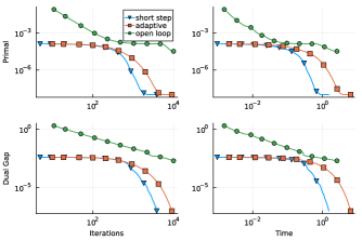
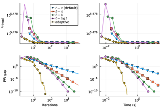
We first show now that our condition (altAdaptive) implies the same primal progress as (adaptive) and then we will show that (altAdaptive) holds for $L$ if $f$ is $L$-smooth. As such all results of Pedregosa et al., (2020) apply readily to the modified variant in Algorithm 5. To demonstrate the convergence behavior of the various step-size strategies we ran a simple test problem with results presented in Figure 10. We see that the adaptive strategy approximates the short step very well and both significantly outperform the open loop strategy.

In the following we present the slightly more involved estimation based on a new progress bound from smoothness. For completeness we also include a significantly simplified estimation based on the regular smoothness bound in Appendix A, however there we only guarantee approximation of the smoothness constant within a factor of $2$. We start with introducing another variant of the smoothness inequality. Note that all these inequalities are equivalent when considering all $x,y$, however we want to apply them for a specific pair of points $x,y$ and then their transformations from one into another might not be sharp as demonstrated in the following remark:

Remark 4.8 (Point-wise smoothness estimations).

Suppose that $f$ is $L$-smooth and convex and consider two points $x,y$. Suppose we want to derive (2.3) from the gradient-based variant in (2.4) using only the two points $x,y$. Then the naive way of doing so it:

$$f(y)-f(x) \leq\mathinner{{}\langle\nabla f(y),y-x\rangle}$$ (convexity)

$$\leq\mathinner{{}\langle\nabla f(x),y-x\rangle}+L\|y-x\|^{2}.$$ (using (2.4))

Observe that this is almost the desired inequality (2.3), except for the smoothness constant $2L$ and not $L$.

The following lemma provides a different smoothness inequality that allows for tighter estimations. It requires $f$ to be $L$-smooth and convex on a potentially slightly larger domain containing $P$.

Lemma 4.9 (Smoothness revisited).

Let $f$ be an $L$-smooth and convex function on the $D$-neighborhood of a compact convex set $P$, where $D$ is the diameter of $P$. Then for all $x,y\in P$ it holds:

$$\frac{\mathinner{{}\langle\nabla f(y)-\nabla f(x),y-x\rangle}^{2}}{2L\|y-x\|^{2}}\leq f(y)-f(x)-\mathinner{{}\langle\nabla f(x),y-x\rangle}.$$ (4.10)

Proof.

As shown in Braun et al., 2022a (, Lemma 1.8), if $f$ is an $L$-smooth convex function on the $D$-neighborhood of a convex set $P$, then for any points $x,y\in P$ it holds

$$\|\nabla f(y)-\nabla f(x)\|^{2}\leq 2L(f(y)-f(x)-\mathinner{{}\langle\nabla f(x),y-x\rangle}).$$ (4.11)

Next we lower bound the left-hand side as

$$\frac{\mathinner{{}\langle\nabla f(y)-\nabla f(x),y-x\rangle}^{2}}{\|y-x\|^{2}}\leq\|\nabla f(y)-\nabla f(x)\|^{2}.$$

Chaining these two inequalities together and rearranging gives the desired claim. ∎

The proof above explicitly relies on the convexity of $f$ via Braun et al., 2022a (, Lemma 1.8). With Lemma 4.9 we can provide the following guarantee on the primal progress.

Lemma 4.10 (Primal progress from (altAdaptive)).

Let $f$ be an $L$-smooth and convex function on the $D$-neighborhood of a compact convex set $P$, where $D$ is the diameter of $P$. Further, let $x_{t+1}=(1-\gamma_{t})x_{t}+\gamma_{t}v_{t}$ with $\gamma_{t}=\min\left\{\frac{\mathinner{{}\langle\nabla f(x_{t}),x_{t}-v_{t}\rangle}}{M\|x_{t}-v_{t}\|^{2}},1\right\}$ for some $M$. If $\mathinner{{}\langle\nabla f(x_{t+1}),x_{t}-v_{t}\rangle}\geq 0$, then it holds:

$$f(x_{t})-f(x_{t+1})\geq\begin{cases*}\frac{\mathinner{{}\langle\nabla f(x_{t}),x_{t}-v_{t}\rangle}^{2}+\mathinner{{}\langle\nabla f(x_{t+1}),x_{t}-v_{t}\rangle}^{2}}{2\max\{L,M\}\|x_{t}-v_{t}\|^{2}}&if \quad$\gamma_{t}\in[0,1]$\\ \frac{\mathinner{{}\langle\nabla f(x_{t}),x_{t}-v_{t}\rangle}}{2}+\frac{\mathinner{{}\langle\nabla f(x_{t+1}),x_{t}-v_{t}\rangle}^{2}}{2\mathinner{{}\langle\nabla f(x_{t}),x_{t}-v_{t}\rangle}}\geq\frac{\mathinner{{}\langle\nabla f(x_{t}),x_{t}-v_{t}\rangle}}{2}&if \quad$\gamma_{t}=1$ and $M\geq L$\end{cases*}.$$

Proof.

If $\gamma_{t}=1$, then without loss of generality we can assume that $M=\frac{\mathinner{{}\langle\nabla f(x_{t}),x_{t}-v_{t}\rangle}}{\|x_{t}-v_{t}\|^{2}}$, as $M$ only occurs in the definition of $\gamma_{t}$ and $x_{t+1}$. Our starting point is Equation (4.10) with $x\leftarrow x_{t+1}$ and $y\leftarrow x_{t}$:

$$f(x_{t})-f(x_{t+1}) \geq\frac{\mathinner{{}\langle\nabla f(x_{t})-\nabla f(x_{t+1}),x_{t}-x_{t+1}\rangle}^{2}}{2L\|x_{t}-x_{t+1}\|^{2}}+\mathinner{{}\langle\nabla f(x_{t+1}),x_{t}-x_{t+1}\rangle}$$

$$=\frac{\mathinner{{}\langle\nabla f(x_{t})-\nabla f(x_{t+1}),x_{t}-v_{t}\rangle}^{2}}{2L\|x_{t}-v_{t}\|^{2}}+\frac{\mathinner{{}\langle\nabla f(x_{t}),x_{t}-v_{t}\rangle}\cdot\mathinner{{}\langle\nabla f(x_{t+1}),x_{t}-v_{t}\rangle}}{M\|x_{t}-v_{t}\|^{2}} x_{t+1} \gamma_{t}$$ (definition of and )

$$\geq\frac{\mathinner{{}\langle\nabla f(x_{t})-\nabla f(x_{t+1}),x_{t}-v_{t}\rangle}^{2}}{2\max\{L,M\}\|x_{t}-v_{t}\|^{2}}+\frac{\mathinner{{}\langle\nabla f(x_{t}),x_{t}-v_{t}\rangle}\cdot\mathinner{{}\langle\nabla f(x_{t+1}),x_{t}-v_{t}\rangle}}{\max\{L,M\}\|x_{t}-v_{t}\|^{2}} \mathinner{{}\langle\nabla f(x_{t+1}),x_{t}-v_{t}\rangle}\geq 0$$ ()

$$=\frac{\mathinner{{}\langle\nabla f(x_{t}),x_{t}-v_{t}\rangle}^{2}+\mathinner{{}\langle\nabla f(x_{t+1}),x_{t}-v_{t}\rangle}^{2}}{2\max\{L,M\}\|x_{t}-v_{t}\|^{2}}.$$

Now if $\gamma_{t}=1$ and $M\geq L$, then the above simplifies to:

$$f(x_{t})-f(x_{t+1})\geq\frac{\mathinner{{}\langle\nabla f(x_{t}),x_{t}-v_{t}\rangle}}{2}+\frac{\mathinner{{}\langle\nabla f(x_{t+1}),x_{t}-v_{t}\rangle}^{2}}{2\mathinner{{}\langle\nabla f(x_{t}),x_{t}-v_{t}\rangle}}\geq\frac{\mathinner{{}\langle\nabla f(x_{t}),x_{t}-v_{t}\rangle}}{2}.$$

This finishes the proof. ∎

Before we continue a few remarks are in order. First of all, observe that

$$f(x_{t})-f(x_{t+1})\geq\frac{\mathinner{{}\langle\nabla f(x_{t}),x_{t}-v_{t}\rangle}^{2}+\mathinner{{}\langle\nabla f(x_{t+1}),x_{t}-v_{t}\rangle}^{2}}{2\max\{L,M\}\|x_{t}-v_{t}\|^{2}},$$

has an additional term compared to the standard smoothness estimation (4.9) and $\mathinner{{}\langle\nabla f(x_{t+1}),x_{t}-v_{t}\rangle}=0$ if and only if $x_{t+1}$ is identical to the line search solution. This is in particular the case if $f$ is a standard quadratic as then the line search solution is identical to the short step solution. Nonetheless, in the typical case this extra term provides additional primal progress. Taking the maximum in the denominator ensures that if $M<L$, then we recover the primal progress that one would have obtained with the estimation $M=L$. This seems counter-intuitive as usually using estimations $M<L$ would lead to overshooting and negative primal progress, however here we still require that (altAdaptive) holds for $M$, which prevents exactly this as can be seen from the proof. In particular, disregarding adaptivity for a second, in the case where $L$ is known, then with the choice $M=L$, Lemma 4.11 provides a stronger primal progress bound compared to (4.9) assuming that (altAdaptive) holds for $L$ (which holds always as $f$ is $L$-smooth; see Lemma 4.11):

$$f(x_{t})-f(x_{t+1})\geq\frac{\mathinner{{}\langle\nabla f(x_{t}),x_{t}-v_{t}\rangle}^{2}+\mathinner{{}\langle\nabla f(x_{t+1}),x_{t}-v_{t}\rangle}^{2}}{2L\|x_{t}-v_{t}\|^{2}}.$$

This improved primal progress bound might give rise to improved convergence rates in some regimes; see also Teboulle and Vaisbourd, (2023) for a similar analysis for the unconstrained case providing optimal constants for the convergence rates of gradient descent. Moreover, the discussion above also implies that if (altAdaptive) holds it might provide more primal progress than the original test via (adaptive) used in Pedregosa et al., (2020).

To conclude, we will now show that (altAdaptive) holds for $L$, whenever the function is $L$-smooth and $\gamma_{t}$ is the corresponding short step for $L$. This implies that both (altAdaptive) and (adaptive) hold for $L$ whenever $f$ is $L$-smooth with the added benefit of numerical stability and additional primal progress via (altAdaptive).

Lemma 4.11 (Smoothness implies (altAdaptive)).

Let $f$ be $L$-smooth. Further, let $x_{t+1}=(1-\gamma_{t})x_{t}+\gamma_{t}v_{t}$ with $\gamma_{t}=\min\left\{\frac{\mathinner{{}\langle\nabla f(x_{t}),x_{t}-v_{t}\rangle}}{L\|x_{t}-v_{t}\|^{2}},1\right\}$. Then (altAdaptive) holds, i.e.,

$$\mathinner{{}\langle\nabla f(x_{t+1}),x_{t}-v_{t}\rangle}\geq 0.$$

Proof.

We use the alternative definition of smoothness using the gradients (2.4), i.e., we have

$$\mathinner{{}\langle\nabla f(y)-\nabla f(x),y-x\rangle}\leq L\|y-x\|^{2}\quad\text{for all }x,y\in P.$$

Now plug in $x\leftarrow x_{t}$ and $y\leftarrow x_{t+1}$, so that we obtain

$$\mathinner{{}\langle\nabla f(x_{t+1})-\nabla f(x_{t}),x_{t+1}-x_{t}\rangle} \leq L\|x_{t+1}-x_{t}\|^{2}$$

and using the definition of $x_{t+1}$ it follows

$$\mathinner{{}\langle\nabla f(x_{t+1})-\nabla f(x_{t}),\gamma_{t}(v_{t}-x_{t})\rangle} \leq L\gamma_{t}^{2}\|v_{t}-x_{t}\|^{2}.$$

Now, if $\gamma_{t}=1$, then $\mathinner{{}\langle\nabla f(x_{t}),x_{t}-v_{t}\rangle}\geq L\|x_{t}-v_{t}\|^{2}$, so that

$$\mathinner{{}\langle\nabla f(x_{t+1})-\nabla f(x_{t}),v_{t}-x_{t}\rangle}\leq\mathinner{{}\langle\nabla f(x_{t}),x_{t}-v_{t}\rangle},$$

holds. Otherwise, if $0<\gamma_{t}<1$, then dividing by $\gamma_{t}$ and plugging in the definition of $\gamma_{t}$ yields

$$\mathinner{{}\langle\nabla f(x_{t+1})-\nabla f(x_{t}),v_{t}-x_{t}\rangle}\leq\mathinner{{}\langle\nabla f(x_{t}),x_{t}-v_{t}\rangle}.$$

In both cases, rearranging gives the desired inequality

$$\mathinner{{}\langle\nabla f(x_{t+1}),x_{t}-v_{t}\rangle}\geq 0.$$

Finally, in case $\gamma_{t}=0$ we have $x_{t}=x_{t+1}$ and the assertion holds trivially. ∎

0   Objective function $f$, smoothness estimate $\widetilde{L}$, feasible points $x$, $v$ with $\mathinner{{}\langle\nabla f(x),x-v\rangle}\geq 0$, progress parameters $\eta\leq 1<\tau$

0   Updated estimate $\widetilde{L}^{*}$, step-size $\gamma$

1   $M\leftarrow\eta\widetilde{L}$

2   loop

3      $\gamma\leftarrow\min\{\mathinner{{}\langle\nabla f(x),x-v\rangle}\mathbin{/}(M\|x-v\|^{2}),1\}$ {compute short step for estimation $M$}

4      if $\mathinner{{}\langle\nabla f(x+\gamma(v-x)),x-v\rangle}\geq 0$ then

5         $\widetilde{L}^{*}\leftarrow M$

6         return  $\widetilde{L}^{*}$, $\gamma$

7      end if

8      $M\leftarrow\tau M$

9   end loop

Algorithm 5 (modified) Adaptive step-size strategy

Remark 4.12 (Faster open loop convergence).

The adaptive step-size strategy from above uses feedback from the function and as such is not of the open loop type. In many applications such adaptive strategies are the strategies of choice as the function feedback is relatively minimal but convergence speed is superior (in most but not all cases as mentioned in Section 4.2). For many important cases we can also obtain improved convergence with rates of higher order for open loop step-sizes by using the modified step-size rule $\gamma_{t}=\frac{\ell}{t+\ell}$ with $\ell\in\mathbb{N}_{\geq 1}$; see Wirth et al., 2023a ; Wirth et al., 2023c for details. This is quite surprising as we only change the shift $\ell$ and not the order of $t$ in the denominator of $\gamma_{t}$. In fact, note that the order of $t$ in the denominator cannot be changed significantly as we need that $\sum_{t}\gamma_{t}=\infty$ and that $\sum_{t}\gamma_{t}^{2}$ converges for the step-size strategy to work; see Braun et al., 2022a . If the corresponding $\ell$ cannot be set in practice, and if it has to be an open loop strategy, $\gamma_{t}=\frac{2+\log(t+1)}{t+2+\log(t+1)}$ works very well; we can use $t$ or $t+1$ in the log depending on whether the first iteration is $t=0$ or $t=1$. This corresponds essentially to a strategy where $\ell$ is gradually increased and it provides accelerated convergence rates when those exist while maintaining the same worst-case convergence rates as the basic strategy $\gamma_{t}=\frac{2}{t+2}$ (Wirth et al., 2023b, ). For a sample computation, see Figure 10.

Figure 9: Convergence speed for a simple quadratic over a $K$-sparse polytope with three different step-size strategies. The basic open loop step-size $\gamma_{t}=\frac{2}{2+t}$, the short step rule, which requires a smoothness estimate $L$ (here we used the exact smoothness), and the adaptive step-size rule that dynamically approximates $L$. Plot is log-log so that the order of the convergence corresponds to different slopes of the trajectories.

Figure 10: Convergence speed for a simple quadratic over a $K$-sparse polytope for open loop strategies of the form $\gamma_{t}=\frac{\ell}{\ell+t}$. We can see that (depending on the specifics of the problem) larger $\ell$ achieve convergence rates of a higher order. For comparison also the adaptive step-size strategy has been included. Plot is log-log so that the order of the convergence corresponds to different slopes of the trajectories.

5 Two applications

In the following we will present two applications of the Frank-Wolfe algorithm. Both examples use very simple quadratic objectives of the form $f(x)=\|x-p\|^{2}$ for some $p$ for the sake of exposition; for more complex examples see also Braun et al., 2022a .

5.1 The Approximate Carathéodory Problem

Our first example, is the Approximate Carathéodory Problem. For this example, the Frank-Wolfe algorithm does not only present a practical means to solve the problem but in fact, its convergence guarantees itself provide a proof of the theorem and optimal bounds for a wide variety of regimes. Here we will confine ourselves to the $2$-norm case not assuming any additional properties, however many more involved cases are possible as studied in Combettes and Pokutta, (2023).

Given a compact convex set $P\subseteq{\mathbb{R}}^{n}$, recall that Carathéodory’s theorem states that any $x^{*}\in P$ can be written as a convex combination of no more than $n+1$ extreme points of $P$, i.e., $x^{*}=\sum_{1\leq i\leq n+1}\lambda_{i}v_{i}$ with $\lambda\geq 0$, $\sum_{i}\lambda_{i}=1$, and $v_{i}$ extreme points of $P$ with $1\leq i\leq n+1$. In the context of Carathéodory’s theorem, the cardinality of a point $x^{*}\in P$, refers to the minimum number of required extreme points to express $x^{*}$ as a convex combination of those. If $x^{*}$ is of low cardinality it is often also referred to as sparse. Every specific convex combination that expresses $x^{*}$ provides an upper bound on the cardinality of $x^{*}$. The approximate variant of Carathéodory’s problem asks: given $x^{*}\in P$, what is required cardinality of an $x\in P$ to approximate $x^{*}$ within an error of no more than $\varepsilon>0$ (in a given norm)? Put differently, we are looking for $x\in P$ with $\|x-x^{*}\|\leq\varepsilon$ of low cardinality. The approximate Carathéodory theorem states:

Theorem 5.1 (Approximate Carathéodory Theorem).

Let $p\geq 2$ and $P$ be a compact convex set. For every $x^{*}\in P$, there exists $x\in P$ with cardinality of no more than $\mathcal{O}(pD_{p}^{2}/\epsilon^{2})$ satisfying $\|x-x^{*}\|_{p}\leq\epsilon$, where $D_{p}=\max_{v,w\in P}\|w-v\|_{p}$ is the $p$-norm diameter of $P$.

Note that the bounds of Theorem 5.1 are essentially tight in many cases (Mirrokni et al.,, 2017). In the following, we briefly discuss the case $p=2$ without any additional assumptions. Suppose we have given a point $x^{*}\in P$ we can consider the objective

$$f(x)\doteq\|x-x^{*}\|^{2}.$$

Further, let $\varepsilon>0$ be the approximation guarantee. Assuming, we have access to an LMO for $P$, we can now minimize the function $f(x)$ over $P$ via the Frank-Wolfe algorithm (Algorithm 4). In order to achieve $\|x-x^{*}\|\leq\varepsilon$ we have to run the Frank-Wolfe algorithm until $f(x_{t})=f(x_{t})-f(x^{*})\leq\varepsilon^{2}$, which by Theorem 4.4 takes no more than $\mathcal{O}(2D^{2}/\epsilon^{2})$ iterations, where $D$ is the $\ell_{2}$-diameter of $P$. Moreover, in each iteration the algorithm is picking up at most one extreme point as discussed in Section 4.1. This establishes the guarantee for case $p=2$ in Theorem 5.1. Here we applied the basic convergence guarantee from Theorem 4.4. However, for the Frank-Wolfe algorithm many more convergence guarantees are known, depending on properties of the feasible domain and position of the point $x^{*}$ that we want to approximate with a sparse convex combination. These improved convergence rates immediately translate into improved approximation guarantees for the approximate Carathéodory problem and we state some of these guarantees in Table 1.

$\ell_{p}$-norm	Assumption	Cardinality bound
$p\in\left[2,+\infty\right[$	–	$\displaystyle\mathcal{O}\!\left(\frac{pD_{p}^{2}}{\epsilon^{2}}\right)$ or $\displaystyle\mathcal{O}\!\left(\frac{p(D_{*}^{2}+D_{0}^{2})}{\epsilon^{2}}\right)$
		($D_{p},D_{0},D_{*}$ diameters; see Combettes and Pokutta, (2023))
	$x^{*}\in\operatorname{ri}(P)$	$\displaystyle\mathcal{O}\!\left(p\left(\frac{D_{p}}{r_{p}}\right)^{2}\ln\!\left(\frac{1}{\epsilon}\right)\right)$
		($\operatorname{ri}(P)$ relative interior, $r_{p}$ radius so that $B^{p}_{r_{p}}(x^{*})\cap\operatorname{aff}(P)\subseteq P$)
	$\alpha_{p}$-strongly convex $P$	$\displaystyle\mathcal{O}\!\left(\frac{\sqrt{p}D_{p}+p/\alpha_{p}}{\epsilon}\right)$
	$(\alpha_{p},q_{p})$-uniformly convex $P$, $q_{p}\in\left[2,+\infty\right[$	$\displaystyle\mathcal{O}\!\left(\frac{(pD_{p}^{2})^{(q_{p}-1)/q_{p}}+p/\alpha_{p}^{2/q_{p}}}{\epsilon^{2(q_{p}-1)/q_{p}}}\right)$
$p\in\left]1,2\right[$	–	$\displaystyle\mathcal{O}\!\left(\frac{n^{(2-p)/p}D_{2}^{2}}{\epsilon^{2}}\right)$
$p=1$	–	$\displaystyle\mathcal{O}\!\left(\frac{nD_{2}^{2}}{\epsilon^{2}}\right)$
		($n$ ambient dimension of $P$, $D_{2}$ is $\ell_{2}$-diameter)
$p=+\infty$	–	$\displaystyle\mathcal{O}\!\left(\frac{D_{2}^{2}}{\epsilon^{2}}\right)$
		($D_{2}$ is $\ell_{2}$-diameter)

Table 1: Cardinality bounds to achieve $\epsilon$-approximation for the approximate Carathéodory problem with respect to the $\ell_{p}$-norm; see Combettes and Pokutta, (2023) for full table. Recall that $P$ is $(\alpha,q)$-uniformly convex if for any $x,y\in P$, $\gamma\in[0,1]$, and $z\in\mathbb{R}^{n}$ with $\|z\|\leq 1$ we have $y+\gamma(x-y)+\gamma(1-\gamma)\cdot\alpha\|x-y\|^{q}z\in P$, where $\alpha$ and $q$ are positive. An $(\alpha/2,2)$-uniformly convex set is called $\alpha$-strongly convex.

Apart from establishing theoretical results by means of the Frank-Wolfe algorithm’s convergence guarantees it can be easily used in actual computations, see e.g., Figures 12 and 12 for an example. Observe that in the particular case of $f(x)$ here, we can also directly observe the primal gap and hence use it as a stopping criterion. The Frank-Wolfe approach to the approximate Carathéodory Problem has been also recently used in Quantum Mechanics to establish new Bell inequalities and local models, as well as improve the Grothendieck constant $K_{G}(3)$ of order $3$ (see Designolle et al., 2023a ; Designolle et al., 2023b and the references contained therein). This approach is also very useful in the context of the coreset problem, which asks for a subset of data points of a large data set that maintains approximately the same statistical properties (see Braun et al., 2022a (, Section 5.2.5)).

Figure 11: Cardinality vs. approximation error in $\ell_{2}$-norm over a polytope of dimension $n=1000$ for the Frank-Wolfe algorithm and two more advanced variants Lazy Away-step Frank-Wolfe (Braun et al., 2019b, ) and Blended Pairwise Conditional Gradients (Tsuji et al.,, 2022). All algorithms use the short step step-size.

Figure 12: Same setup as in Figure 12, however the step-size strategy is the adaptive strategy from Section 4.5. As we can see the Frank-Wolfe algorithm is quite sensitive to the strategy while more advanced variants, due to their design of only adding new vertices when not enough progress can be made otherwise, are not.

5.2 Separating hyperplanes

In Section 5.1 we have used the Frank-Wolfe algorithm for obtaining a convex decomposition of a point $x^{*}\in P$, i.e., we certified membership in $P$. We can also use the Frank-Wolfe algorithm with the same objective $f(x)=\|x-\tilde{x}\|^{2}$ to obtain separating hyperplanes for points $\tilde{x}\not\in P$, i.e., we certify non-membership. This has been successfully applied in Designolle et al., 2023a ; Designolle et al., 2023b to certify that the correlations of certain quantum states exhibit non-locality, i.e., are truly quantum by separating them from the local polytope, the polytope of all classical correlations. Moreover, it has also been used in Thuerck et al., (2023) to derive separating hyperplanes from enumeration oracles.

In the following we provide the most naive way of computing separating hyperplanes. An improved strategy has been presented in Thuerck et al., (2023), which derives a new algorithmic characterization of non-membership, that requires fewer iterations of the Frank-Wolfe algorithm compared to our naive strategy here. It is also interesting to note that from a complexity-theoretic perspective, what the Frank-Wolfe algorithm does is to turn an LMO for $P$ into a separation oracle for $P$ via optimizing the objective $\|x-\tilde{x}\|^{2}$.

Given $\tilde{x}\not\in P$, we consider the optimization problem

$$\min_{x\in P}\|x-\tilde{x}\|^{2},$$ (Sep)

with $f(x)\doteq\|x-\tilde{x}\|^{2}$. Using Lemma 4.2 we can immediately obtain a separating hyperplane from an optimal solution $x^{*}\in P$ to (Sep):

$$\mathinner{{}\langle\nabla f(x^{*}),x^{*}\rangle}\leq\mathinner{{}\langle\nabla f(x^{*}),v\rangle},$$ (sepHyperplane)

which holds for all $v\in P$. Moreover, as $\tilde{x}\not\in P$, we have by convexity $\mathinner{{}\langle\nabla f(x^{*}),x^{*}-\tilde{x}\rangle}\geq f(x^{*})-f(\tilde{x})=f(x^{*})>0$. and hence (sepHyperplane) is violated by $\tilde{x}$, i.e., $\mathinner{{}\langle\nabla f(x^{*}),x^{*}\rangle}>\mathinner{{}\langle\nabla f(x^{*}),\tilde{x}\rangle}$. This argument provides the desired separating hyperplane mathematically, but numerically it is problematic as we usually solve Problem (Sep) only up to some accuracy $\varepsilon>0$, typically using the Frank-Wolfe gap $\max_{v\in P}\mathinner{{}\langle\nabla f(x_{t}),x_{t}-v\rangle}\leq\varepsilon$ as stopping criterion. When the algorithm stops we similarly obtain

$$\mathinner{{}\langle\nabla f(x_{t}),x_{t}\rangle}-\varepsilon\leq\mathinner{{}\langle\nabla f(x_{t}),x\rangle}\quad\text{ which simplifies to }\quad\min_{v\in P}\mathinner{{}\langle\nabla f(x_{t}),v\rangle}\leq\mathinner{{}\langle\nabla f(x_{t}),x\rangle},$$ (validIneq)

which is valid for all $x\in P$. However this inequality does not necessarily separate $\tilde{x}$ from $P$. A sufficient condition for separation is that $\tilde{x}$ is $\sqrt{\varepsilon}$-far from $P$ so that we have $\|x^{*}-\tilde{x}\|>\sqrt{\varepsilon}$. We then can use the same convexity argument as before:

$$\mathinner{{}\langle\nabla f(x_{t}),x_{t}-\tilde{x}\rangle}-\varepsilon$$ (stopping criterion)

$$\geq \;f(x_{t})-f(\tilde{x})-\varepsilon$$ (convexity)

$$\geq \;f(x^{*})-\varepsilon>0. \|x^{*}-\tilde{x}\|>\sqrt{\varepsilon}$$ ()

Now turning this argument around, if $\tilde{x}\not\in P$ is $\varepsilon$-far from $P$, we need to run the Frank-Wolfe algorithm until the Frank-Wolfe gap satisfies $\max_{v\in P}\mathinner{{}\langle\nabla f(x_{t}),x_{t}-v\rangle}\leq\varepsilon^{2}$. Combining this with Theorem 4.5 we can estimate

$$\frac{6.75LD^{2}}{t+2}\leq\varepsilon^{2},$$

with $L=2$. Thus we have found a separating hyperplane for $\tilde{x}$ whenever $t\geq 13.5D^{2}/\varepsilon^{2}$.

In practice however we usually do not know $D$ and we also do not know how far $\tilde{x}$ is from $P$. Nonetheless, we can simply test in each iteration $t$ whether $\tilde{x}$ violates (validIneq), i.e.,

$$\nabla f(x_{t})\text{ separates }\tilde{x}\quad\Leftrightarrow\quad\min_{v\in P}\mathinner{{}\langle\nabla f(x_{t}),v\rangle}>\mathinner{{}\langle\nabla f(x_{t}),\tilde{x}\rangle}.$$

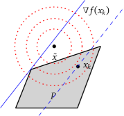
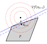
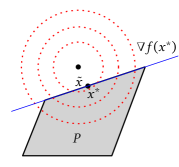
and simply stop then and are guaranteed this will take no more than $\mathcal{O}(D^{2}/\varepsilon^{2})$ iterations. The process is illustrated in Figure 13. A similar approach, basically combining Sections 5.1 and 5.2 can also be used to compute the intersection of two compact convex sets or certify their disjointness by means of a separating hyperplane (assuming LMO access to each) as shown in Braun et al., 2022b .

Figure 13: Each iterate $x_{k}$ induces a valid inequality of the form $\min_{v\in P}\mathinner{{}\langle\nabla f(x_{t}),v\rangle}\leq\mathinner{{}\langle\nabla f(x_{t}),x\rangle}$ in blue (dashed blue line is $\nabla f(x_{t})$ at $x_{t}$), which may or may not separate $\tilde{x}$; see middle and left respectively. At $x^{*}$ the induced inequality $\min_{v\in P}\mathinner{{}\langle\nabla f(x^{*}),v\rangle}=\mathinner{{}\langle\nabla f(x^{*}),x^{*}\rangle}\leq\mathinner{{}\langle\nabla f(x^{*}),x\rangle}$ is guaranteed to separate $\tilde{x}\not\in P$ and often (but not always) induces a facet of $P$.

6 Computational codes

For actual computations we have developed the FrankWolfe.jl Julia package, which implements many Frank-Wolfe variants and is highly customizable. Moreover, we have also developed a mixed-integer extension Boscia.jl that allows for some of the variables taking discrete values.

A Adaptive Step-sizes: Simpler estimation

In this section we will present a simplified estimation of Section 4.5 for adaptive step-sizes albeit at the cost being only able to approximate the smoothness of $f$ within a factor of $2$. The basic setup is identical to the one before, however we use a different test for accepting the estimation $M$ of $L$:

$$\mathinner{{}\langle\nabla f(x_{t+1}),x_{t}-v_{t}\rangle}\geq\frac{1}{2}\mathinner{{}\langle\nabla f(x_{t}),x_{t}-v_{t}\rangle},$$ (altAdaptive-simple)

where $x_{t+1}=(1-\gamma_{t})x_{t}+\gamma_{t}v_{t}$ as before with $\gamma_{t}=\min\left\{\frac{\mathinner{{}\langle\nabla f(x_{t}),x_{t}-v_{t}\rangle}}{M\|x_{t}-v_{t}\|^{2}},1\right\}$ being the short step for the estimation $M$ and the corresponding algorithm becomes Algorithm 6 in this case. We proceed similarly as before: we first show that condition (altAdaptive-simple) implies primal progress and then we will show that (altAdaptive-simple) holds for $2L$ if $f$ is $L$-smooth; this is were (altAdaptive-simple) is weaker than (altAdaptive).

Lemma A.1 (Primal progress from (altAdaptive-simple)).

Let $x_{t+1}=(1-\gamma_{t})x_{t}+\gamma_{t}v_{t}$ with $\gamma_{t}=\min\left\{\frac{\mathinner{{}\langle\nabla f(x_{t}),x_{t}-v_{t}\rangle}}{M\|x_{t}-v_{t}\|^{2}},1\right\}$ for some $M$. If $\mathinner{{}\langle\nabla f(x_{t+1}),x_{t}-v_{t}\rangle}\geq\frac{1}{2}\mathinner{{}\langle\nabla f(x_{t}),x_{t}-v_{t}\rangle}$, then it holds:

$$f(x_{t})-f(x_{t+1})\geq\gamma_{t}\mathinner{{}\langle\nabla f(x_{t}),x_{t}-v_{t}\rangle}/2=\begin{cases*}\frac{\mathinner{{}\langle\nabla f(x_{t}),x_{t}-v_{t}\rangle}^{2}}{2M\|x_{t}-v_{t}\|^{2}}&if \quad$\gamma_{t}\in[0,1)$\\ \mathinner{{}\langle\nabla f(x_{t}),x_{t}-v_{t}\rangle}/2&if \quad$\gamma_{t}=1$\end{cases*}.$$

Proof.

The proof follows directly via convexity and plugging in the definitions:

$$f(x_{t})-f(x_{t+1}) \geq\mathinner{{}\langle\nabla f(x_{t+1}),x_{t}-x_{t+1}\rangle}$$ (convexity)

$$\geq\gamma_{t}\mathinner{{}\langle\nabla f(x_{t+1}),x_{t}-v_{t}\rangle} x_{t+1}$$ (definition of )

$$\geq\gamma_{t}\mathinner{{}\langle\nabla f(x_{t}),x_{t}-v_{t}\rangle}/2$$ (assumption of (altAdaptive-simple))

$$=\begin{cases*}\frac{\mathinner{{}\langle\nabla f(x_{t}),x_{t}-v_{t}\rangle}^{2}}{2M\|x_{t}-v_{t}\|^{2}}&if \quad$\gamma_{t}\in[0,1)$\\ \mathinner{{}\langle\nabla f(x_{t}),x_{t}-v_{t}\rangle}/2&if \quad$\gamma_{t}=1$\end{cases*}. \gamma_{t}$$ (definition of )

∎

Note that the proof above (again) explicitly relies on the convexity of $f$. It remains to show that (altAdaptive-simple) holds for $2L$, whenever the function is $L$-smooth and $\gamma_{t}$ is the corresponding short step for $M=2L$. The proof is very similar to before, however the last step is different.

Lemma A.2 (Smoothness implies (altAdaptive-simple)).

Let $f$ be $L$-smooth. Further, let $x_{t+1}=(1-\gamma_{t})x_{t}+\gamma_{t}v_{t}$ with $\gamma_{t}=\min\left\{\frac{\mathinner{{}\langle\nabla f(x_{t}),x_{t}-v_{t}\rangle}}{M\|x_{t}-v_{t}\|^{2}},1\right\}$ and $M=2L$. Then (altAdaptive-simple) holds, i.e.,

$$\mathinner{{}\langle\nabla f(x_{t+1}),x_{t}-v_{t}\rangle}\geq\frac{1}{2}\mathinner{{}\langle\nabla f(x_{t}),x_{t}-v_{t}\rangle}.$$

Proof.

We use the alternative definition of smoothness using the gradients, i.e., we have

$$\mathinner{{}\langle\nabla f(y)-\nabla f(x),y-x\rangle}\leq L\|y-x\|^{2}\quad\text{for all }x,y\in P,$$

by Remark 2.3. Now plug in $x\leftarrow x_{t}$ and $y\leftarrow x_{t+1}$, so that we obtain

$$\mathinner{{}\langle\nabla f(x_{t+1})-\nabla f(x_{t}),x_{t+1}-x_{t}\rangle} \leq L\|x_{t+1}-x_{t}\|^{2}$$

and with plugging in the definition of $x_{t+1}$ we obtain

$$\mathinner{{}\langle\nabla f(x_{t+1})-\nabla f(x_{t}),\gamma_{t}(v_{t}-x_{t})\rangle} \leq L\gamma_{t}^{2}\|v_{t}-x_{t}\|^{2}.$$

If $\gamma_{t}>0$, dividing by $\gamma_{t}$ and then plugging in the definition of $\gamma_{t}$ yields

$$\mathinner{{}\langle\nabla f(x_{t+1})-\nabla f(x_{t}),v_{t}-x_{t}\rangle}\leq\frac{1}{2}\mathinner{{}\langle\nabla f(x_{t}),x_{t}-v_{t}\rangle},$$

and rearranging gives the desired inequality

$$\mathinner{{}\langle\nabla f(x_{t+1}),x_{t}-v_{t}\rangle}\geq\frac{1}{2}\mathinner{{}\langle\nabla f(x_{t}),x_{t}-v_{t}\rangle}.$$

In case $\gamma_{t}=0$ we have $x_{t}=x_{t+1}$ and the assertion holds trivially. ∎

We will now show that (altAdaptive-simple) is indeed weaker than (altAdaptive) and that we cannot replace $M=L$ in Lemma 4.11. To this end consider the following $1$-dimensional example: Pick $f(x)\doteq x^{2}$, so that $L=2$ holds. Consider $f:[-1,1]\mapsto\mathbb{R}$ and $x_{t}=1$. Then we have $\nabla f(x_{t})=2$, $v_{t}=-1$, and

$$\frac{\mathinner{{}\langle\nabla f(x_{t}),x_{t}-v_{t}\rangle}}{L\|x_{t}-v_{t}\|^{2}}=\frac{2(1-(-1))}{2(1-(-1))^{2}}=\frac{1}{2},$$

so that $\gamma_{t}=\min\left\{\frac{\mathinner{{}\langle\nabla f(x_{t}),x_{t}-v_{t}\rangle}}{L\|x_{t}-v_{t}\|^{2}},1\right\}=\frac{1}{2}$, $x_{t+1}=0$, and $\nabla f(x_{t+1})=0$. This contradicts $0=\mathinner{{}\langle\nabla f(x_{t+1}),x_{t}-v_{t}\rangle}\geq\frac{1}{2}\mathinner{{}\langle\nabla f(x_{t}),x_{t}-v_{t}\rangle}>0$.

0   Objective function $f$, smoothness estimate $\widetilde{L}$, feasible points $x$, $v$ with $\mathinner{{}\langle\nabla f(x),x-v\rangle}\geq 0$, progress parameters $\eta\leq 1<\tau$

0   Updated estimate $\widetilde{L}^{*}$, step-size $\gamma$

1   $M\leftarrow\eta\widetilde{L}$

2   loop

3      $\gamma\leftarrow\min\{\mathinner{{}\langle\nabla f(x),x-v\rangle}\mathbin{/}(M\|x-v\|^{2}),1\}$ {compute short step for estimation $M$}

4      if $\mathinner{{}\langle\nabla f(x+\gamma(v-x)),x-v\rangle}\geq\frac{1}{2}\mathinner{{}\langle\nabla f(x),x-v\rangle}$ then

5         $\widetilde{L}^{*}\leftarrow M$

6         return  $\widetilde{L}^{*}$, $\gamma$

7      end if

8      $M\leftarrow\tau M$

9   end loop

Algorithm 6 (modified) Adaptive step-size strategy - simple variant

References

- Anari et al., (2019) Anari, N., Haghtalab, N., Naor, S., Pokutta, S., Singh, M., and Torrico, A. (2019). Structured Robust Submodular Maximization: Offline and Online Algorithms. Proceedings of AISTATS.
- Anari et al., (2021) Anari, N., Haghtalab, N., Naor, S., Pokutta, S., Singh, M., and Torrico, A. (2021). Structured Robust Submodular Maximization: Offline and Online Algorithms. INFORMS Journal on Computing, 33:1259–1684.
- Bach, (2015) Bach, F. (2015). Duality between subgradient and conditional gradient methods. SIAM Journal on Optimization, 25(1):115–129.
- Bach, (2019) Bach, F. (2019). Submodular functions: From discrete to continuous domains. Mathematical Programming, 175:419–459.
- Badanidiyuru and Vondrák, (2014) Badanidiyuru, A. and Vondrák, J. (2014). Fast algorithms for maximizing submodular functions. In Proceedings of the 25th Annual ACM-SIAM Symposium on Discrete Algorithms (SODA), pages 1497–1514.
- Bolte et al., (2007) Bolte, J., Daniilidis, A., and Lewis, A. (2007). The Łojasiewicz inequality for nonsmooth subanalytic functions with applications to subgradient dynamical systems. SIAM Journal on Optimization, 17(4):1205–1223.
- Bomze et al., (2021) Bomze, I. M., Rinaldi, F., and Zeffiro, D. (2021). Frank–Wolfe and friends: A journey into projection-free first-order optimization methods. 4OR A Quarterly Journal of Operations Research, 19:313–345.
- Boyd et al., (2004) Boyd, S., Boyd, S. P., and Vandenberghe, L. (2004). Convex Optimization. Cambridge University Press, Cambridge.
- (9) Braun, G., Carderera, A., Combettes, C. W., Hassani, H., Karbasi, A., Mokthari, A., and Pokutta, S. (2022a). Conditional gradient methods. preprint available at https://arxiv.org/abs/2211.14103.
- (10) Braun, G. and Pokutta, S. (2015a). The matching polytope does not admit fully-polynomial size relaxation schemes. Proceeedings of SODA.
- (11) Braun, G. and Pokutta, S. (2015b). The matching polytope does not admit fully-polynomial size relaxation schemes. IEEE Transactions on Information Theory, 61(10):1–11.
- Braun and Pokutta, (2021) Braun, G. and Pokutta, S. (2021). Dual Prices for Frank-Wolfe Algorithms. preprint available at https://arxiv.org/abs/2101.02087.
- (13) Braun, G., Pokutta, S., Tu, D., and Wright, S. (2019a). Blended Conditional Gradients: the unconditioning of conditional gradients. Proceedings of ICML.
- (14) Braun, G., Pokutta, S., and Weismantel, R. (2022b). Alternating Linear Minimization: Revisiting von Neumann’s alternating projections. preprint.
- Braun et al., (2017) Braun, G., Pokutta, S., and Zink, D. (2017). Lazifying Conditional Gradient Algorithms. Proceedings of the International Conference on Machine Learning (ICML).
- (16) Braun, G., Pokutta, S., and Zink, D. (2019b). Lazifying Conditional Gradient Algorithms. Journal of Machine Learning Research (JMLR), 20(71):1–42.
- Carderera and Pokutta, (2020) Carderera, A. and Pokutta, S. (2020). Second-order Conditional Gradient Sliding. preprint available at https://arxiv.org/abs/2002.08907.
- Carderera et al., (2021) Carderera, A., Pokutta, S., Schütte, C., and Weiser, M. (2021). CINDy: Conditional gradient-based Identification of Non-linear Dynamics – Noise-robust recovery. preprint available at https://arxiv.org/abs/2101.02630.
- Chen et al., (2018) Chen, L., Harshaw, C., Hassani, H., and Karbasi, A. (2018). Projection-free online optimization with stochastic gradient: From convexity to submodularity. In Proceedings of the 35th International Conference on Machine Learning (ICML), volume 80, pages 814–823. PMLR.
- Chen and Sun, (2023) Chen, Z. and Sun, Y. (2023). Reducing discretization error in the Frank–Wolfe method. preprint available at https://arxiv.org/abs/2304.01432.
- Cheung and Li, (2018) Cheung, E. and Li, Y. (2018). Solving separable nonsmooth problems using Frank–Wolfe with uniform affine approximations. In Proceedings of the 27th International Joint Conference on Artificial Intelligence (IJCAI), IJCAI’18, pages 2035–2041. AAAI Press.
- Clarkson, (2010) Clarkson, K. L. (2010). Coresets, sparse greedy approximation, and the Frank–Wolfe algorithm. ACM Transactions on Algorithms, 6(4):1–30.
- Combettes and Pokutta, (2020) Combettes, C. W. and Pokutta, S. (2020). Boosting Frank-Wolfe by Chasing Gradients. Proceedings of ICML.
- Combettes and Pokutta, (2021) Combettes, C. W. and Pokutta, S. (2021). Complexity of Linear Minimization and Projection on Some Sets. Operations Research Letters, 49.
- Combettes and Pokutta, (2023) Combettes, C. W. and Pokutta, S. (2023). Revisiting the Approximate Carathéodory Problem via the Frank-Wolfe Algorithm. Mathematical Programming A, 197:191—214.
- Dahik, (2021) Dahik, C. (2021). Robust Discrete Optimization Under Ellipsoidal Uncertainty. PhD thesis, Bourgogne Franche-Comté.
- Dantzig, (1981) Dantzig, G. B. (1981). Reminiscences about the origins of linear programming. Technical report, Stanford University, CA. Systems Optimization Lab.
- Dantzig, (1983) Dantzig, G. B. (1983). Reminiscences about the Origins of Linear Programming, pages 78–86. Springer, Berlin.
- de Oliveira, (2023) de Oliveira, W. (2023). Short paper – A note on the Frank–Wolfe algorithm for a class of nonconvex and nonsmooth optimization problems. Open Journal of Mathematical Optimization, 4:1–10.
- (30) Designolle, S., Iommazzo, G., Besançon, M., Knebel, S., Gelß, P., and Pokutta, S. (2023a). Improved local models and new Bell inequalities via Frank-Wolfe algorithms. Physical Reviews Research, 5.
- (31) Designolle, S., Vértesi, T., and Pokutta, S. (2023b). Symmetric multipartite Bell inequalities via Frank-Wolfe algorithms. preprint available at https://arxiv.org/abs/2310.20677.
- Dvurechensky et al., (2020) Dvurechensky, P., Ostroukhov, P., Safin, K., Shtern, S., and Staudigl, M. (2020). Self-concordant analysis of Frank–Wolfe algorithms. In III, H. D. and Singh, A., editors, Proceedings of the 37th International Conference on Machine Learning, volume 119 of Proceedings of Machine Learning Research, pages 2814–2824. PMLR.
- Feldman et al., (2011) Feldman, M., Naor, J. S., and Schwartz, R. (2011). A unified continuous greedy algorithm for submodular maximization. In Proceedings of the 52nd Annual Symposium on Foundations of Computer Science (FOCS), pages 570–579. IEEE.
- Frank and Wolfe, (1956) Frank, M. and Wolfe, P. (1956). An algorithm for quadratic programming. Naval Research Logistics Quarterly, 3(1–2):95–110.
- Freund et al., (2017) Freund, R. M., Grigas, P., and Mazumder, R. (2017). An extended Frank–Wolfe method with “in-face” directions, and its application to low-rank matrix completion. SIAM Journal on Optimization, 27(1):319–346.
- Garber, (2020) Garber, D. (2020). Revisiting Frank–Wolfe for polytopes: Strict complementarity and sparsity. In Larochelle, H., Ranzato, M., Hadsell, R., Balcan, M. F., and Lin, H., editors, Advances in Neural Information Processing Systems (NeurIPS), volume 33, pages 18883–18893. Curran Associates, Inc.
- Garber and Hazan, (2015) Garber, D. and Hazan, E. (2015). Faster rates for the Frank–Wolfe method over strongly-convex sets. In Bach, F. and Blei, D., editors, Proceedings of the 32nd International Conference on Machine Learning (ICML), volume 37, pages 541–549. PMLR.
- Garber and Hazan, (2016) Garber, D. and Hazan, E. (2016). A linearly convergent variant of the conditional gradient algorithm under strong convexity, with applications to online and stochastic optimization. SIAM Journal on Optimization, 26(3):1493–1528.
- Garber and Kretzu, (2021) Garber, D. and Kretzu, B. (2021). Revisiting projection-free online learning: The strongly convex case. In Banerjee, A. and Fukumizu, K., editors, Proceedings of The 24th International Conference on Artificial Intelligence and Statistics, volume 130 of Proceedings of Machine Learning Research, pages 3592–3600. PMLR.
- Garber and Wolf, (2021) Garber, D. and Wolf, N. (2021). Frank–Wolfe with a nearest extreme point oracle. In Belkin, M. and Kpotufe, S., editors, Proceedings of Thirty Fourth Conference on Learning Theory, volume 134 of Proceedings of Machine Learning Research, pages 2103–2132. PMLR.
- Gilbert, (1966) Gilbert, E. G. (1966). An iterative procedure for computing the minimum of a quadratic form on a convex set. SIAM Journal on Control, 4(1):61–80.
- GuéLat and Marcotte, (1986) GuéLat, J. and Marcotte, P. (1986). Some comments on Wolfe’s ‘away step’. Mathematical Programming, 35(1):110–119.
- Gupta et al., (2016) Gupta, S., Goemans, M., and Jaillet, P. (2016). Solving combinatorial games using products, projections and lexicographically optimal bases. preprint available at https://arxiv.org/abs/1603.00522.
- Harchaoui et al., (2015) Harchaoui, Z., Juditsky, A., and Nemirovski, A. S. (2015). Conditional gradient algorithms for norm-regularized smooth convex optimization. Mathematical Programming, 152:75–112.
- Hassani et al., (2017) Hassani, H., Soltanolkotabi, M., and Karbasi, A. (2017). Gradient methods for submodular maximization. In Guyon, I., Luxburg, U. V., Bengio, S., Wallach, H., Fergus, R., Vishwanathan, S., and Garnett, R., editors, Advances in Neural Information Processing Systems (NIPS), volume 30, pages 5841–5851. Curran Associates, Inc.
- Hazan and Kale, (2012) Hazan, E. and Kale, S. (2012). Projection-free online learning. In Proceedings of the 29th International Conference on Machine Learning (ICML), pages 1843–1850, Madison, WI. Omnipress.
- Hazan and Minasyan, (2020) Hazan, E. and Minasyan, E. (2020). Faster projection-free online learning. In Abernethy, J. and Agarwal, S., editors, Proceedings of Thirty Third Conference on Learning Theory, volume 125 of Proceedings of Machine Learning Research, pages 1877–1893. PMLR.
- Jaggi, (2013) Jaggi, M. (2013). Revisiting Frank–Wolfe: Projection-free sparse convex optimization. In Dasgupta, S. and McAllester, D., editors, Proceedings of the 30th International Conference on Machine Learning, volume 28 of ICML’13, pages 427–435, Atlanta, Georgia, USA. PMLR.
- Jing et al., (2023) Jing, N., Fang, E. X., and Tang, C. Y. (2023). Robust matrix estimations meet Frank–Wolfe algorithm. Machine Learning, pages 1–38.
- Joulin et al., (2014) Joulin, A., Tang, K., and Fei-Fei, L. (2014). Efficient image and video co-localization with Frank–Wolfe algorithm. In Proceedings of European Conference on Computer Vision (ECCV), volume 8694 of Lecture Notes in Computer Science, pages 253–268. Springer.
- Kerdreux et al., (2021) Kerdreux, T., Roux, C., d’Aspremont, A., and Pokutta, S. (2021). Linear Bandits on Uniformly Convex Sets. Journal of Machine Learning Research (JMLR), 22:1–23.
- Lacoste-Julien, (2016) Lacoste-Julien, S. (2016). Convergence rate of Frank–Wolfe for non-convex objectives. HAL hal-01415335.
- Lacoste-Julien and Jaggi, (2015) Lacoste-Julien, S. and Jaggi, M. (2015). On the global linear convergence of Frank–Wolfe optimization variants. In Cortes, C., Lawrence, N. D., Lee, D. D., Sugiyama, M., and Garnett, R., editors, Advances in Neural Information Processing Systems (NIPS), volume 28, pages 496–504. Curran Associates.
- Lacoste-Julien et al., (2013) Lacoste-Julien, S., Jaggi, M., Schmidt, M., and Pletscher, P. (2013). Block-coordinate Frank–Wolfe optimization for structural SVMs. In Dasgupta, S. and McAllester, D., editors, Proceedings of the 30th International Conference on Machine Learning, volume 28 of Proceedings of Machine Learning Research, pages 53–61. PMLR.
- Lan, (2013) Lan, G. (2013). The complexity of large-scale convex programming under a linear optimization oracle. Technical report, Department of Industrial and Systems Engineering, University of Florida.
- Lan et al., (2017) Lan, G., Pokutta, S., Zhou, Y., and Zink, D. (2017). Conditional Accelerated Lazy Stochastic Gradient Descent. Proceedings of the International Conference on Machine Learning (ICML).
- Levitin and Polyak, (1966) Levitin, E. S. and Polyak, B. T. (1966). Constrained minimization methods. USSR Computational Mathematics and Mathematical Physics, 6(5):1–50.
- Macdonald et al., (2022) Macdonald, J., Besançon, M., and Pokutta, S. (2022). Interpretable Neural Networks with Frank-Wolfe: Sparse Relevance Maps and Relevance Orderings. Proceedings of ICML.
- Mirrokni et al., (2017) Mirrokni, V., Leme, R. P., Vladu, A., and Wong, S. C.-w. (2017). Tight bounds for approximate Carathéodory and beyond. In Precup, D. and Teh, Y. W., editors, Proceedings of the 34th International Conference on Machine Learning (ICML), volume 70 of Proceedings of Machine Learning Research, pages 2440–2448. PMLR.
- Mirzasoleiman et al., (2016) Mirzasoleiman, B., Badanidiyuru, A., and Karbasi, A. (2016). Fast constrained submodular maximization: Personalized data summarization. In Balcan, M. F. and Weinberger, K. Q., editors, Proceedings of the 33nd International Conference on Machine Learning (ICML), volume 48 of Proceedings of Machine Learning Research, pages 1358–1367. PMLR.
- (61) Mokhtari, A., Hassani, H., and Karbasi, A. (2018a). Conditional gradient method for stochastic submodular maximization: Closing the gap. In Storkey, A. and Perez-Cruz, F., editors, Proceedings of the Twenty-First International Conference on Artificial Intelligence and Statistics, volume 84 of Proceedings of Machine Learning Research, pages 1886–1895. PMLR.
- (62) Mokhtari, A., Hassani, H., and Karbasi, A. (2018b). Decentralized submodular maximization: Bridging discrete and continuous settings. In Dy, J. and Krause, A., editors, Proceedings of the 35th International Conference on MachineLearning, volume 80 of Proceedings of Machine Learning Research, pages 3616–3625. PMLR.
- Moondra et al., (2021) Moondra, J., Mortagy, H., and Gupta, S. (2021). Reusing combinatorial structure: Faster iterative projections over submodular base polytopes. In Ranzato, M., Beygelzimer, A., Dauphin, Y., Liang, P., and Vaughan, J. W., editors, Advances in Neural Information Processing Systems, volume 34, pages 25386–25399. Curran Associates, Inc.
- Négiar et al., (2020) Négiar, G., Dresdner, G., Tsai, A. Y.-T., El Ghaoui, L., Locatello, F., Freund, R. M., and Pedregosa, F. (2020). Stochastic Frank–Wolfe for constrained finite-sum minimization. In III, H. D. and Singh, A., editors, Proceedings of the 37th International Conference on Machine Learning (ICML), volume 119 of Proceedings of Machine Learning Research, pages 7253–7262. PMLR.
- Nemirovski and Yudin, (1983) Nemirovski, A. S. and Yudin, D. B. (1983). Problem Complexity and Method Efficiency in Optimization. Wiley.
- Nesterov, (2004) Nesterov, Y. E. (2004). Introductory Lectures on Convex Optimization: A Basic Course, volume 87 of Applied Optimization. Springer, 1 edition.
- Nesterov, (2018) Nesterov, Y. E. (2018). Lectures on Convex Optimization, volume 137 of Optimization and Its Applications. Springer.
- Nocedal and Wright, (2006) Nocedal, J. and Wright, S. J. (2006). Numerical Optimization. Springer Series in Operations Research and Financial Engineering. Springer, 2 edition.
- Pedregosa et al., (2020) Pedregosa, F., Negiar, G., Askari, A., and Jaggi, M. (2020). Linearly convergent Frank–Wolfe with backtracking line-search. In Chiappa, S. and Calandra, R., editors, Proceedings of the 23rd International Conference on Artificial Intelligence and Statistics, (AISTATS), volume 108 of Proceedings of Machine Learning Research, pages 1–10. PMLR.
- Pierucci et al., (2014) Pierucci, F., Harchaoui, Z., and Malick, J. (2014). A smoothing approach for composite conditional gradient with nonsmooth loss. In Conférence d’Apprentissage Automatique (CAp).
- Potra and Wright, (2000) Potra, F. A. and Wright, S. J. (2000). Interior-point methods. Journal of Computational and Applied Mathematics, 124(1–2):281–302.
- Ravi et al., (2019) Ravi, S. N., Collins, M. D., and Singh, V. (2019). A deterministic nonsmooth Frank Wolfe algorithm with coreset guarantees. INFORMS Journal on Optimization, 1(2):120–142.
- Rothvoss, (2017) Rothvoss, T. (2017). The matching polytope has exponential extension complexity. Journal of the ACM, 64(6):41:1–19.
- Sinha, (2018) Sinha, M. (2018). Lower bounds for approximating the matching polytope. In Proceedings of the Twenty-Ninth Annual ACM-SIAM Symposium on Discrete Algorithms, pages 1585–1604. SIAM.
- Tang et al., (2014) Tang, K., Joulin, A., Li, L.-J., and Fei-Fei, L. (2014). Co-localization in real-world images. In Proceedings of the IEEE Conference on Computer Vision and Pattern Recognition (CVPR), pages 1464–1471.
- Teboulle and Vaisbourd, (2023) Teboulle, M. and Vaisbourd, Y. (2023). An elementary approach to tight worst case complexity analysis of gradient based methods. Mathematical Programming, 201(1-2):63–96.
- Thuerck et al., (2023) Thuerck, D., Sofranac, B., Pfetsch, M., and Pokutta, S. (2023). Learning Cuts via Enumeration Oracles. to appear in Proceedings of NeurIPS.
- Tsuji et al., (2022) Tsuji, K., Tanaka, K., and Pokutta, S. (2022). Pairwise Conditional Gradients without Swap Steps and Sparser Kernel Herding. Proceedings of ICML.
- Vondrák, (2008) Vondrák, J. (2008). Optimal approximation for the submodular welfare problem in the value oracle model. In Proceedings of the 40th Annual ACM Symposium on Theory of Computing (STOC), pages 67–74.
- Wäldchen et al., (2022) Wäldchen, S., Huber, F., and Pokutta, S. (2022). Training Characteristic Functions with Reinforcement Learning: XAI-methods play Connect Four. Proceedings of ICML.
- Wang et al., (2016) Wang, Y.-X., Sadhanala, V., Dai, W., Neiswanger, W., Sra, S., and Xing, E. P. (2016). Parallel and distributed block-coordinate Frank–Wolfe algorithms. In Proceedings of the 33rd International Conference on Machine Learning (ICML), volume 48, pages 1548–1557. PMLR.
- (82) Wirth, E., Kerdreux, T., and Pokutta, S. (2023a). Acceleration of Frank-Wolfe algorithms with open loop step-sizes. Proceedings of AISTATS.
- (83) Wirth, E., Peña, J., and Pokutta, S. (2023b). A new open-loop strategy for Frank-Wolfe algorithms. in preparation.
- (84) Wirth, E., Peña, J., and Pokutta, S. (2023c). Accelerated Affine-Invariant Convergence Rates of the Frank-Wolfe Algorithm with Open-Loop Step-Sizes. preprint available at https://arxiv.org/abs/2310.04096.
- Wolfe, (1970) Wolfe, P. (1970). Convergence theory in nonlinear programming. In Integer and Nonlinear Programming, pages 1–36. North-Holland.
- Zhang et al., (2023) Zhang, W., Shi, Y., Zhang, B., and Yuan, D. (2023). Dynamic regret of distributed online Frank–Wolfe convex optimization.
- Zhang et al., (2017) Zhang, W., Zhao, P., Zhu, W., Hoi, S. C. H., and Zhang, T. (2017). Projection-free distributed online learning in networks. In Precup, D. and Teh, Y. W., editors, Proceedings of the 34th International Conference on Machine Learning (ICML), volume 70 of Proceedings of Machine Learning Research, pages 4054–4062. PMLR.