Strongly clustered random graphs via triadic closure: An exactly solvable model

Lorenzo Cirigliano Dipartimento di Fisica Università “Sapienza”, P.le A. Moro, 2, I-00185 Rome, Italy. Centro Ricerche Enrico Fermi, Piazza del Viminale, 1, I-00184 Rome, Italy    Claudio Castellano Istituto dei Sistemi Complessi (ISC-CNR), Via dei Taurini 19, I-00185 Rome, Italy Centro Ricerche Enrico Fermi, Piazza del Viminale, 1, I-00184 Rome, Italy    Gareth J. Baxter Departamento de Física da Universidade de Aveiro & I3N, Campus Universitário de Santiago, 3810-193 Aveiro, Portugal    Gábor Timár Departamento de Física da Universidade de Aveiro & I3N, Campus Universitário de Santiago, 3810-193 Aveiro, Portugal
Abstract

Triadic closure, the formation of a connection between two nodes in a network sharing a common neighbor, is considered a fundamental mechanism determining the clustered nature of many real-world topologies. In this work we define a static triadic closure (STC) model for clustered networks, whereby starting from an arbitrary fixed backbone network, each triad is closed independently with a given probability. Assuming a locally treelike backbone we derive exact expressions for the expected number of various small, loopy motifs (triangles, 444-loops, diamonds and 444-cliques) as a function of moments of the backbone degree distribution. In this way we determine how transitivity and its suitably defined generalizations for higher-order motifs depend on the heterogeneity of the original network, revealing the existence of transitions due to the interplay between topologically inequivalent triads in the network. Furthermore, under reasonable assumptions for the moments of the backbone network, we establish approximate relationships between motif densities, which we test in a large dataset of real-world networks. We find a good agreement, indicating that STC is a realistic mechanism for the generation of clustered networks, while remaining simple enough to be amenable to analytical treatment.

I Introduction

A network representation is a powerful tool for studying a huge variety of complex systems. Random network models, such as the Erdős-Rényi model [1, 2], the more general configuration model [3, 4, 5] and its various extensions [6] have enjoyed considerable popularity due to their amenability to mathematical analysis. These random networks have a locally treelike structure in the infinite size limit, which facilitates the study of branching processes (e.g., percolation, epidemic spreading) and interacting systems (e.g., the Ising model) on top of these substrates [7].

An important feature of many real-world networks is a non-vanishing density of short loops, in particular triangles [8], which is at significant odds with the locally treelike structure assumption. The propensity of node triads to form triangles is often quantified by the local clustering coefficient or the global transitivity [6]. While the presence of clustering in networks has significant effects on processes such as percolation and epidemics [9, 10, 11], both the mean local clustering coefficient and the transitivity tend to zero in the infinite size limit of locally treelike random networks. To account for non-vanishing clustering, i.e., a non-vanishing density of triangles in the infinite size limit, Strauss [12] proposed an exponential random graph model with soft constraints on the number of edges and the number of triangles in the network. One may introduce further constraints to achieve specific network structures [13, 14, 15, 16]. Although such models are easily generalizable and rather flexible, their use is impeded by the highly non-trivial phase diagrams that can emerge [17], making it difficult to fit real network structures and to study dynamical models.

The latter problem is circumvented in a model proposed by Newman [18] where each node belongs to a prescribed number of partial cliques (fully connected subgraphs where edges are removed with a certain probability) whose sizes are randomly distributed. Since the building blocks—the partial cliques—only overlap at nodes and not at edges, this model allows for analytical treatment using generating functions to study percolation and related processes. The same approach is used in Refs. [19, 20] where each node is prescribed an edge-degree and a triangle-degree, and nodes are randomly joined together in pairs to form edges (as in the original configuration model) and randomly joined together in groups of three to form triangles. Using only triangles and no higher-order cliques allows for better control over the degree distribution to fit real network data. In an elegant approach Gleeson [21] is able to fit an arbitrary degree distribution and clustering spectrum CKsubscript𝐶𝐾C_{K} (the mean clustering coefficient of nodes of degree K𝐾K) by prescribing an appropriate joint degree and clique size distribution. The modelling approach of randomly connecting cliques or partial cliques may be generalized to randomly connecting arbitrary subgraphs [22]. As long as these subgraphs only overlap at nodes, standard generating function techniques can be used to solve for various network properties such as percolation.

Most real network structures cannot be accurately described by the above random graph models due to the complex overlapping patterns of clustered subgraphs. A very simple and reasonably realistic mechanism—particularly in social networks—that is able to produce high clustering and complex community structure is triadic closure [23]. The idea is that as a network evolves many new links are created between nodes that share a common neighbour, i.e., by closing triads. Triadic closure is widely considered to be an essential mechanism of structure formation in social networks [24, 25, 26, 27, 28, 29, 30, 31, 32, 33, 34]. Most existing models of network formation involving triadic closure are dynamic in nature, that is, the triadic closure mechanism is generally part of a growth or rewiring process. This often makes it difficult to obtain an analytical description and to identify what network features may be directly attributed to triadic closure.

Here we consider a minimal static model of triadic closure, whereby given an existing (backbone) network, a fraction f𝑓f of existing triads is, on average, closed. In the case of a configuration model backbone this model can be seen as a special case of a more general model recently considered in Ref. [35]. There, triadic closure was applied after creating a network with community structure and degree correlations, using a generalized configuration model. For f=1𝑓1f=1 static triadic closure implies that all nodes at distance 222 in the backbone become nearest neighbors in the new network. Hence a process involving nearest neighbors on the new clustered network is equivalent to the same process with an extended range of interaction in the original backbone network [36].

The simplicity of this model allows for a detailed analytical description, which is lacking in most of the studies involving triadic closure. By means of the generating function formalism we derive exact results in the case where the original backbone is locally treelike. In particular, network transitivity and densities of other higher-order motifs (such as diamonds or loops of length 4) are expressed in terms of moments of the backbone degree distribution. In this way we uncover the existence of sharp transitions in clustering properties of the model as a function of the heterogeneity of the backbone. The origin of these transitions is traced to the competition between topologically distinct types of subgraphs created by the closure process. A comparison between the model predictions and a large database of networks confirms the plausibility of static triadic closure as a generative mechanism for many real-world structures.

II Model description

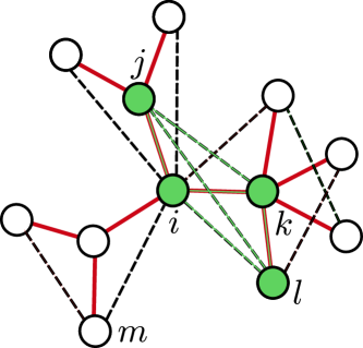
Given a graph 𝒢=(𝒱,)𝒢𝒱\mathcal{G}=(\mathcal{V},\mathcal{E}) with N=|𝒱|𝑁𝒱N=|\mathcal{V}| nodes and E=||𝐸E=|\mathcal{E}| edges, a triad centered on node j𝑗j is a sequence of three consecutive nodes (i,j,k)=(k,j,i)𝑖𝑗𝑘𝑘𝑗𝑖(i,j,k)=(k,j,i), i.e. an unoriented path of length two made by the edges (i,j),(j,k)𝑖𝑗𝑗𝑘(i,j),(j,k)\in\mathcal{E}. A triangle {i,j,k}𝑖𝑗𝑘\{i,j,k\} is a closed undirected path of length three. Note that for each triangle there are three distinct closed triads. We define the static triadic closure (STC) mechanism as a random process in which each triad becomes a triangle with probability f𝑓f through the addition of an edge joining its end nodes. Using this STC mechanism, it is possible to build a graph in the following way. We start from a network 𝒢0=(𝒱,0)subscript𝒢0𝒱subscript0\mathcal{G}_{0}=(\mathcal{V},\mathcal{E}_{0}) and we write down all the triads in it. For each triad (i,j,k)𝑖𝑗𝑘(i,j,k), we update the edge set 0subscript0\mathcal{E}_{0} by adding to it the edge (i,k)𝑖𝑘(i,k) with probability f𝑓f. When the triadic closure has been attempted on all the triads in 𝒢0subscript𝒢0\mathcal{G}_{0}, the process ends. The result is a new edge list fsubscript𝑓\mathcal{E}_{f} with Ef=|f|subscript𝐸𝑓subscript𝑓E_{f}=|\mathcal{E}_{f}| edges, from which we can define a new network 𝒢f=(𝒱,f)subscript𝒢𝑓𝒱subscript𝑓\mathcal{G}_{f}=(\mathcal{V},\mathcal{E}_{f}) with a rich variety of short loops and highly complex structure (see FIG. 1). This algorithm defines an ensemble of random networks, which we will refer to, with a slight abuse of notation, as 𝒢fsubscript𝒢𝑓\mathcal{G}_{f}.

This algorithm may describe quite different specific mechanisms for triadic closure. One could imagine for instance a triadic closure process in which a node is inclined to be connected with one of its second neighbors with probability ψ𝜓\psi, but the triangle is only closed if both nodes agree. This would correspond to a probability of triadic closure f=ψ2𝑓superscript𝜓2f=\psi^{2}. Alternatively, the triad (i,j,k)𝑖𝑗𝑘(i,j,k) may be closed if at least one among i𝑖i and k𝑘k likes the other, the resulting triadic closure probability is f=1(1ψ)2𝑓1superscript1𝜓2f=1-(1-\psi)^{2}. In both cases, the STC process described as above works with the prescription of using the appropriate probability in place of f𝑓f.

It is worth remarking that our definition of static triadic closure is fully general: it is possible to generate, using this STC mechanism, random clustered networks starting from any given backbone. In the following sections however, we study the ensemble of graphs 𝒢fsubscript𝒢𝑓\mathcal{G}_{f}, generated by static triadic closure starting from a random, uncorrelated locally treelike backbone 𝒢0subscript𝒢0\mathcal{G}_{0}, generated using the Uncorrelated Configuration Model [37, 38] with a prescribed degree distribution pksubscript𝑝𝑘p_{k}. We develop the theoretical framework to characterize these STC random graphs, using generating functions to describe the properties of 𝒢fsubscript𝒢𝑓\mathcal{G}_{f} (see Appendix A.1 for general definitions). Exploiting the local treelikeness of the network 𝒢0subscript𝒢0\mathcal{G}_{0}, it is possible to compute average quantities in 𝒢fsubscript𝒢𝑓\mathcal{G}_{f} in terms of averages with respect to pksubscript𝑝𝑘p_{k}. Note that in our model there are two distinct and independent sources of randomness: the first is the random nature of the backbone 𝒢0subscript𝒢0\mathcal{G}_{0}, and the second is the random nature of the STC process.

We will denote with lower-case letters quantities which refer to the backbone 𝒢0subscript𝒢0\mathcal{G}_{0}, and with capital letters quantities related to the graph 𝒢fsubscript𝒢𝑓\mathcal{G}_{f}. In particular k,r,g0(z),g1(z)𝑘𝑟subscript𝑔0𝑧subscript𝑔1𝑧k,r,g_{0}(z),g_{1}(z) and K,R,G0(z),G1(z)𝐾𝑅subscript𝐺0𝑧subscript𝐺1𝑧K,R,G_{0}(z),G_{1}(z) denote the degree, excess degree and the corresponding probability generating functions, in the networks 𝒢0subscript𝒢0\mathcal{G}_{0} and 𝒢fsubscript𝒢𝑓\mathcal{G}_{f}, respectively.

Refer to caption
Figure 1: Pictorial representation of the STC algorithm. The edges of the backbone network 𝒢0subscript𝒢0\mathcal{G}_{0}, a tree with N=12𝑁12N=12 nodes and E0=11subscript𝐸011E_{0}=11 edges, are represented with solid red lines; the dashed black lines represent the edges created by the STC procedure. The result is a network 𝒢fsubscript𝒢𝑓\mathcal{G}_{f} with N=12𝑁12N=12 nodes and Ef=21subscript𝐸𝑓21E_{f}=21 edges, a variety of short loops and a much more complex structure: many new triads, such as (j,i,l)𝑗𝑖𝑙(j,i,l) and (m,i,l)𝑚𝑖𝑙(m,i,l), and many triangles, such as {i,k,l}𝑖𝑘𝑙\{i,k,l\}, are created, as well as other higher-order motifs, for instance 444-loops – unoriented closed paths of length 444, e.g. {i,j,k,l}𝑖𝑗𝑘𝑙\{i,j,k,l\} – and 444-cliques (e.g., the one formed by the nodes shaded in green).

III The generating function of the degree distribution

We begin the study of the network ensemble 𝒢fsubscript𝒢𝑓\mathcal{G}_{f} by investigating the behavior of its degree distribution PK(f)subscript𝑃𝐾𝑓P_{K}(f). For the sake of brevity, we will omit the explicit dependence on f𝑓f of PK(f)subscript𝑃𝐾𝑓P_{K}(f) by writing PKsubscript𝑃𝐾P_{K}. Even if we are not able to compute PKsubscript𝑃𝐾P_{K} explicitly, it is possible to determine its generating function G0(z)subscript𝐺0𝑧G_{0}(z) by expressing it in terms of the generating functions of the degree and of the excess degree distributions in the network 𝒢0subscript𝒢0\mathcal{G}_{0}, g0(z)subscript𝑔0𝑧g_{0}(z) and g1(z)subscript𝑔1𝑧g_{1}(z), respectively. The result we obtain relies on the fact that the generating function of a sum of independent random variables is the product of their generating functions.

Consider first the case f=1𝑓1f=1. K𝐾K is the random variable representing the degree of a node in 𝒢1subscript𝒢1\mathcal{G}_{1}. Assume that this node has degree k𝑘k in 𝒢0subscript𝒢0\mathcal{G}_{0}, and label with i=1,,k𝑖1𝑘i=1,\dots,k its first neighbors. We can write K=k+i=1kri𝐾𝑘superscriptsubscript𝑖1𝑘subscript𝑟𝑖K=k+\sum_{i=1}^{k}r_{i}, where risubscript𝑟𝑖r_{i} is the excess degree of first neighbor i𝑖i. Since the network 𝒢0subscript𝒢0\mathcal{G}_{0} is uncorrelated, the generating function of the variable K𝐾K, conditioned on having degree k𝑘k in 𝒢0subscript𝒢0\mathcal{G}_{0}, is given by [zg1(z)]ksuperscriptdelimited-[]𝑧subscript𝑔1𝑧𝑘[zg_{1}(z)]^{k}. Averaging then over the degree distribution pksubscript𝑝𝑘p_{k} we get G0(z)=g0(zg1(z))subscript𝐺0𝑧subscript𝑔0𝑧subscript𝑔1𝑧G_{0}(z)=g_{0}(zg_{1}(z)). This standard argument can be generalized to arbitrary f𝑓f by considering K=k+i=1kni𝐾𝑘superscriptsubscript𝑖1𝑘subscript𝑛𝑖K=k+\sum_{i=1}^{k}n_{i}, where nisubscript𝑛𝑖n_{i} are random variables, ranging from 00 to risubscript𝑟𝑖r_{i}, representing the number of new connections made with second neighbors in the i𝑖i-th branch. The variables nisubscript𝑛𝑖n_{i} are independent random variables distributed according to binomial distributions B(i)(n;ri,f)=(rin)fn(1f)rinsuperscript𝐵𝑖𝑛subscript𝑟𝑖𝑓binomialsubscript𝑟𝑖𝑛superscript𝑓𝑛superscript1𝑓subscript𝑟𝑖𝑛B^{(i)}(n;r_{i},f)={r_{i}\choose n}f^{n}(1-f)^{r_{i}-n}. We can now repeat the argument used for f=1𝑓1f=1 by simply conditioning not only on k𝑘k, but also on r1,,rksubscript𝑟1subscript𝑟𝑘r_{1},\dots,r_{k}. Hence, for fixed k,r1,,rk𝑘subscript𝑟1subscript𝑟𝑘k,r_{1},\dots,r_{k}, we get zki=1k[(1f+fz)ri]superscript𝑧𝑘superscriptsubscriptproduct𝑖1𝑘delimited-[]superscript1𝑓𝑓𝑧subscript𝑟𝑖z^{k}\prod_{i=1}^{k}[(1-f+fz)^{r_{i}}], where (1f+fz)risuperscript1𝑓𝑓𝑧subscript𝑟𝑖(1-f+fz)^{r_{i}} is the generating function of the binomial distribution B(i)(ni,ri;f)superscript𝐵𝑖subscript𝑛𝑖subscript𝑟𝑖𝑓B^{(i)}(n_{i},r_{i};f). Averaging over the excess degree distributions qr1,,qrksubscript𝑞subscript𝑟1subscript𝑞subscript𝑟𝑘q_{r_{1}},\dots,q_{r_{k}} and over pksubscript𝑝𝑘p_{k} we finally get for the generating function of the degree distribution PKsubscript𝑃𝐾P_{K} in 𝒢fsubscript𝒢𝑓\mathcal{G}_{f}

G0(z)=g0(zg1(1f+fz)).subscript𝐺0𝑧subscript𝑔0𝑧subscript𝑔11𝑓𝑓𝑧G_{0}(z)=g_{0}\big{(}zg_{1}(1-f+fz)\big{)}. (1)

The degree distribution PKsubscript𝑃𝐾P_{K} may be computed, at least in principle, from Eq. (1) by differentiation, since G0(z)=PKzKsubscript𝐺0𝑧subscript𝑃𝐾superscript𝑧𝐾G_{0}(z)=\sum P_{K}z^{K}, see Appendix A.2. Unfortunately, this cannot be done explicitly in a closed form for a generic pksubscript𝑝𝑘p_{k}111It is possible to obtain an exact expression for PKsubscript𝑃𝐾P_{K} if the backbone is a random regular network.. However, in general it is possible to obtain asymptotic estimates of PKsubscript𝑃𝐾P_{K} for large K𝐾K. For instance, if 𝒢0subscript𝒢0\mathcal{G}_{0} has a power-law (PL) degree distribution pkkγsimilar-tosubscript𝑝𝑘superscript𝑘𝛾p_{k}\sim k^{-\gamma}, the resulting 𝒢fsubscript𝒢𝑓\mathcal{G}_{f} is a PL network with PKKγsimilar-tosubscript𝑃𝐾superscript𝐾superscript𝛾P_{K}\sim K^{-\gamma^{\prime}}, with γ=γ1superscript𝛾𝛾1\gamma^{\prime}=\gamma-1, that is the exponent is decreased by one (see Appendix A.2.1 for details).

From the generating function in Eq. (1) we can compute every moment Kndelimited-⟨⟩superscript𝐾𝑛\langle K^{n}\rangle. In particular, the average degree in 𝒢fsubscript𝒢𝑓\mathcal{G}_{f} is given by

Kdelimited-⟨⟩𝐾\displaystyle\langle K\rangle =G0(1)=k+fk(k1),absentsuperscriptsubscript𝐺01delimited-⟨⟩𝑘𝑓delimited-⟨⟩𝑘𝑘1\displaystyle=G_{0}^{\prime}(1)=\langle k\rangle+f\langle k(k-1)\rangle, (2)

which simply states that, on average, each node is connected to a fraction f𝑓f of its second neighbors, reflecting the basic mechanism of static triadic closure. It is important to notice that if 𝒢0subscript𝒢0\mathcal{G}_{0} is a truly sparse graph, that is if k=𝒪(1)delimited-⟨⟩𝑘𝒪1\langle k\rangle=\mathcal{O}(1), see [39], the STC procedure creates a truly sparse graph 𝒢fsubscript𝒢𝑓\mathcal{G}_{f} only if k2=𝒪(1)delimited-⟨⟩superscript𝑘2𝒪1\langle k^{2}\rangle=\mathcal{O}(1). In some cases, such as PL with γ<3𝛾3\gamma<3, k2=𝒪(Nα)delimited-⟨⟩superscript𝑘2𝒪superscript𝑁𝛼\langle k^{2}\rangle=\mathcal{O}(N^{\alpha}) for some 0<α<10𝛼10<\alpha<1, and hence K=𝒪(Nα)delimited-⟨⟩𝐾𝒪superscript𝑁𝛼\langle K\rangle=\mathcal{O}(N^{\alpha}). Models defined on such networks with a slowly diverging mean degree may exhibit a qualitatively different critical behavior from the truly sparse case, see for instance [36].

It is useful to define the factorial moments μnsubscript𝜇𝑛\mu_{n} by

μn=k(k1)(kn+1)=g0(n)(1)subscript𝜇𝑛delimited-⟨⟩𝑘𝑘1𝑘𝑛1superscriptsubscript𝑔0𝑛1\mu_{n}=\langle k(k-1)\dots(k-n+1)\rangle=g_{0}^{(n)}(1) (3)

(see Appendix A.3 for more details).

IV Clustering

Armed with the generating function for the final degree distribution, we may study the various properties of the new network. Since it is the principal motivation for the model, we begin by studying clustering properties, the presence of triangles in the network.

We first focus on the global clustering coefficient of the network 𝒢fsubscript𝒢𝑓\mathcal{G}_{f}, also called transitivity, which is the ratio between three times the total number of triangles to the number of triads in the network. We then discuss the behavior of the mean local clustering coefficient which is the ratio between the number of triangles connected to and the number of triads centered on a particular node, averaged over all nodes.

IV.1 Transitivity

The global clustering coefficient is defined as [38]

T=3NN,𝑇3subscript𝑁subscript𝑁T=\frac{3N_{\triangle}}{N_{\wedge}}, (4)

where Nsubscript𝑁N_{\triangle} and Nsubscript𝑁N_{\wedge} denote the average total number of triangles and triads, respectively222The factor 333 takes into account the fact that in each triangle there are three distinct triads..

IV.1.1 General results

Exploiting the local treelikeness of the underlying backbone network, it is possible to exactly compute the transitivity of the network 𝒢fsubscript𝒢𝑓\mathcal{G}_{f}.

The average number of triads in 𝒢fsubscript𝒢𝑓\mathcal{G}_{f} can be evaluated easily. Take a node of degree K𝐾K in 𝒢fsubscript𝒢𝑓\mathcal{G}_{f}. To form a triad, we can pick one among K𝐾K of its neighbors, and then one among K1𝐾1K-1 remaining other neighbors: hence such a node is the center of K(K1)/2𝐾𝐾12K(K-1)/2 different triads. Averaging over the degree distribution PKsubscript𝑃𝐾P_{K} we get

Nsubscript𝑁\displaystyle N_{\wedge} =N(K2)=N2G0′′(1)absent𝑁delimited-⟨⟩binomial𝐾2𝑁2superscriptsubscript𝐺0′′1\displaystyle=N\left\langle{K\choose 2}\right\rangle=\frac{N}{2}G_{0}^{\prime\prime}(1)
=N2[g0′′(1)(1+fg1(1))2+2fg0′′(1)+f2g0′′′(1)]absent𝑁2delimited-[]superscriptsubscript𝑔0′′1superscript1𝑓subscriptsuperscript𝑔1122𝑓subscriptsuperscript𝑔′′01superscript𝑓2superscriptsubscript𝑔0′′′1\displaystyle=\frac{N}{2}\left[g_{0}^{\prime\prime}(1)(1+fg^{\prime}_{1}(1))^{2}+2fg^{\prime\prime}_{0}(1)+f^{2}g_{0}^{\prime\prime\prime}(1)\right]
=N2[μ2(1+fμ2/μ1)2+2fμ2+f2μ3],absent𝑁2delimited-[]subscript𝜇2superscript1𝑓subscript𝜇2subscript𝜇122𝑓subscript𝜇2superscript𝑓2subscript𝜇3\displaystyle=\frac{N}{2}\left[\mu_{2}(1+f\mu_{2}/\mu_{1})^{2}+2f\mu_{2}+f^{2}\mu_{3}\right], (5)

where we express the average over PKsubscript𝑃𝐾P_{K} in terms of the derivatives of the generating function G0(z)subscript𝐺0𝑧G_{0}(z) and we use Eq. (1).

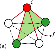
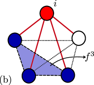
To compute the average total number of triangles we can proceed in the following way. Consider a node i𝑖i of degree k𝑘k in 𝒢0subscript𝒢0\mathcal{G}_{0}, and consider its neighborhood. We evaluate the average number of triangles that are created in its neighborhood, and then average over the degree distribution pksubscript𝑝𝑘p_{k}. With the help of FIG. 2, it is easy to see that triangles in the neighborhood of node i𝑖i can be of only two types: either they are made by joining two neighbors of node i𝑖i via the triadic closure process, with probability f𝑓f (type A); or they are made by joining together three neighbors of node i𝑖i, with probability f3superscript𝑓3f^{3} (type B). Since both these types are defined with reference to the node i𝑖i, one may verify that the triangles will only be counted once. The average number of triangles of type A is fk(k1)/2𝑓𝑘𝑘12fk(k-1)/2, while the average number of triangles of type B is f3k(k1)(k2)/3!superscript𝑓3𝑘𝑘1𝑘23f^{3}k(k-1)(k-2)/3!, hence summing these two contributions together and averaging over pksubscript𝑝𝑘p_{k} we obtain

Nsubscript𝑁\displaystyle N_{\triangle} =Nf6[3μ2+f2μ3].absent𝑁𝑓6delimited-[]3subscript𝜇2superscript𝑓2subscript𝜇3\displaystyle=\frac{Nf}{6}\left[3\mu_{2}+f^{2}\mu_{3}\right]. (6)

Substituting into Eq. (4) we get

T𝑇\displaystyle T =f(3μ2+f2μ3)μ2(1+fμ2/μ1)2+2fμ2+f2μ3.absent𝑓3subscript𝜇2superscript𝑓2subscript𝜇3subscript𝜇2superscript1𝑓subscript𝜇2subscript𝜇122𝑓subscript𝜇2superscript𝑓2subscript𝜇3\displaystyle=\frac{f(3\mu_{2}+f^{2}\mu_{3})}{\mu_{2}(1+f\mu_{2}/\mu_{1})^{2}+2f\mu_{2}+f^{2}\mu_{3}}. (7)

For Erdős-Rényi (ER) backbones, since μn=cnsubscript𝜇𝑛superscript𝑐𝑛\mu_{n}=c^{n}, Eq. (7) reduces to

T=3f+f3c1+2f(1+c)+f2c(1+c).𝑇3𝑓superscript𝑓3𝑐12𝑓1𝑐superscript𝑓2𝑐1𝑐T=\frac{3f+f^{3}c}{1+2f(1+c)+f^{2}c(1+c)}. (8)

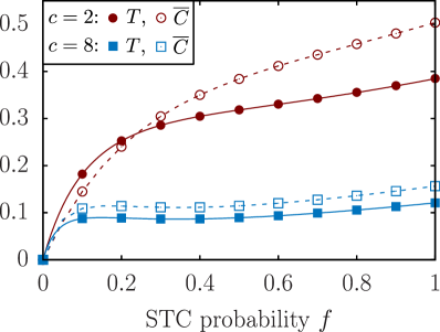
In FIG. 3 we compare Eq. (8) with numerical simulations of 𝒢fsubscript𝒢𝑓\mathcal{G}_{f} networks created from an ER backbone, for different values of the original mean degree c𝑐c and of the closing probability f𝑓f. It is worth noting the non-monotonic behavior of T(f)𝑇𝑓T(f) for large, fixed c𝑐c: for c>c=5.7531𝑐superscript𝑐5.7531c>c^{*}=5.7531..., T(f)𝑇𝑓T(f) admits a maximum and a minimum in the interval [0,1]01[0,1]. This implies that from the same backbone with c>c𝑐superscript𝑐c>c^{*}, we can create two graphs 𝒢f1subscript𝒢subscript𝑓1\mathcal{G}_{f_{1}} and 𝒢f2subscript𝒢subscript𝑓2\mathcal{G}_{f_{2}} having the same transitivity and f1f2subscript𝑓1subscript𝑓2f_{1}\neq f_{2}.

Refer to caption
Refer to caption
Figure 2: A visualization of the triangle counting. Consider node i𝑖i of degree k=4𝑘4k=4, coloured in red, and its neighbors. The edges in 𝒢0subscript𝒢0\mathcal{G}_{0} are represented with solid red lines, while the black dotted lines are the edges that may be created by the STC mechanism and hence may appear in 𝒢fsubscript𝒢𝑓\mathcal{G}_{f}. We can distinguish between triangles of type A – shaded in green in (a) – made of two already existing edges and one new edge, and triangles of type B – shaded blue in (b) – made of three new edges. The total number of potential A-triangles is (42)=6binomial426{4\choose 2}=6, i.e. the number of edges in the 444-clique composed of i𝑖i’s neighbors, and each one of them is created with probability f𝑓f. Over many STC realizations, there are 6f6𝑓6f of them on average. The total number of potential B-triangles is (43)=4binomial434{4\choose 3}=4, i.e., the number of triangles in the 444-clique composed of i𝑖i’s neighbors. Each one of them appears with probability f3superscript𝑓3f^{3}, hence on average there are 4f34superscript𝑓34f^{3} of them. The average number of triangles for a node of degree k=4𝑘4k=4 is then 6f+4f36𝑓4superscript𝑓36f+4f^{3}. Repeating this argument for all nodes we obtain Eq. (6). Note that in this way each triangle is counted exactly once.
Refer to caption
Figure 3: Transitivity T𝑇T (filled symbols) and mean local clustering coefficient C¯¯𝐶\overline{C} (empty symbols) as a function of f𝑓f in networks 𝒢fsubscript𝒢𝑓\mathcal{G}_{f} generated from ER backbones with mean degree c=2𝑐2c=2 (circles), c=8𝑐8c=8 (squares) and size N=106𝑁superscript106N=10^{6}, averaged over 101010 realizations of the STC procedure. The continuous lines correspond to the exact expression for the transitivity in Eq. (8) and they are in perfect agreement with simulation results. Dashed lines are not an analytic solution but simply a guide to the eye.

IV.1.2 The case of power-law backbones

The case of 𝒢fsubscript𝒢𝑓\mathcal{G}_{f} generated from power-law (PL) degree distributed backbones 𝒢0subscript𝒢0\mathcal{G}_{0} with pkkγsimilar-tosubscript𝑝𝑘superscript𝑘𝛾p_{k}\sim k^{-\gamma} is of particular interest. We assume that k[kmin,kc(N)]𝑘subscript𝑘minsubscript𝑘𝑐𝑁k\in[k_{\text{min}},k_{c}(N)], and that the maximum degree grows as a power of N𝑁N whose value depends on the exponent γ𝛾\gamma: kc(N)Nω(γ)similar-tosubscript𝑘𝑐𝑁superscript𝑁𝜔𝛾k_{c}(N)\sim N^{\omega(\gamma)}\to\infty as N𝑁N\to\infty [37], with 0<ω1/20𝜔120<\omega\leq 1/2 for 2<γ32𝛾32<\gamma\leq 3 and ω=1/(γ1)𝜔1𝛾1\omega=1/(\gamma-1) for γ>3𝛾3\gamma>3. Some moments of a power-law distribution diverge in the infinite-size limit, depending on the value of γ𝛾\gamma (see Appendix B). This implies that, for some values of γ𝛾\gamma, Nsubscript𝑁N_{\triangle} and Nsubscript𝑁N_{\wedge} may grow faster than linearly in N𝑁N 333Of course, 3NN3subscript𝑁subscript𝑁3N_{\triangle}\leq N_{\wedge} always.. A careful analysis of Eq. (7) can be carried out, using the fact that, when the factorial moments diverge, they are dominated by the leading term, hence μnknsimilar-tosubscript𝜇𝑛delimited-⟨⟩superscript𝑘𝑛\mu_{n}\sim\langle k^{n}\rangle, so that they can be used to stand in for the moments of the degree distribution. Expressions for them are given in Appendix B. For γ>4𝛾4\gamma>4 none of the terms appearing in Eq. (7) diverge in the limit of infinite network size, and the transitivity is a nonlinear function of f𝑓f and γ𝛾\gamma which can be computed using the expressions for μnsubscript𝜇𝑛\mu_{n} in Eqs.(49)-(52). More interesting is the case γ4𝛾4\gamma\leq 4, in which some of the terms in Eq. (7) diverge. We get, in the limit kcsubscript𝑘𝑐k_{c}\to\infty,

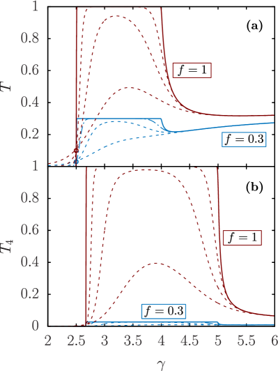
T{0 for 2<γ<5/2,f1+c(kmin) for γ=5/2,f for 5/2<γ4,similar-to-or-equals𝑇cases0 for 2𝛾52𝑓1𝑐subscript𝑘min for 𝛾52𝑓 for 52𝛾4T\simeq\begin{cases}0&\text{ for }2<\gamma<5/2,\\ \frac{f}{1+c(k_{\text{min}})}&\text{ for }\gamma=5/2,\\ f&\text{ for }5/2<\gamma\leq 4,\\ \end{cases} (9)

where c(kmin)𝑐subscript𝑘minc(k_{\text{min}}) is a constant, depending only on kminsubscript𝑘mink_{\text{min}}, given by the ratio of the diverging moments μ23/(μ3μ12)superscriptsubscript𝜇23subscript𝜇3superscriptsubscript𝜇12\mu_{2}^{3}/(\mu_{3}\mu_{1}^{2}) evaluated at γ=5/2𝛾52\gamma=5/2. Within the continuous degree approximation (see Appendix B) c(kmin)=3kmin𝑐subscript𝑘min3subscript𝑘minc(k_{\text{min}})=3k_{\text{min}}. Eq. (9) reveals a discontinuity in T𝑇T at γ=5/2𝛾52\gamma=5/2, as observed in FIG. 4(a). This discontinuous behavior occurs because, while the number of triangles is asymptotically k3delimited-⟨⟩superscript𝑘3\langle k^{3}\rangle, the number of triads is asymptotically proportional to k23+ak3superscriptdelimited-⟨⟩superscript𝑘23𝑎delimited-⟨⟩superscript𝑘3\langle k^{2}\rangle^{3}+a\langle k^{3}\rangle, where a𝑎a is a constant. At γ=5/2𝛾52\gamma=5/2 the dominant term in the number of triads changes, causing the abrupt transition observed in T𝑇T.

Refer to caption
Figure 4: Analytical expressions for (a) transitivity, Eq. (7), and (b) 444-transitivity, Eq. (22) for n=4𝑛4n=4, in STC networks with a PL backbone, as a function of γ𝛾\gamma, for two different values of the STC probability f𝑓f. These curves are obtained evaluating Eqs. (7), (22) within a continuous degree approximation, with kmin=3subscript𝑘min3k_{\text{min}}=3. Continuous lines correspond to the infinite-size limit kcsubscript𝑘𝑐k_{c}\to\infty, dashed lines are for kc=103,105,1010subscript𝑘𝑐superscript103superscript105superscript1010k_{c}=10^{3},10^{5},10^{10}. Circles in panel (a) correspond to the values for γ=5/2𝛾52\gamma=5/2 given in Eq. (9).

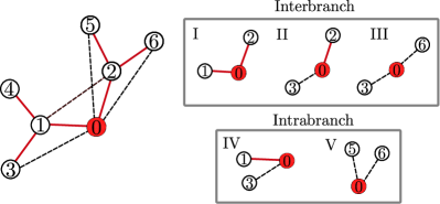
To understand this dual behavior of the number of triads, we identify five classes of topologically different triads in 𝒢fsubscript𝒢𝑓\mathcal{G}_{f}. Denoting with i0subscript𝑖0i_{0} the center node of the triad (i1,i0,i2)subscript𝑖1subscript𝑖0subscript𝑖2(i_{1},i_{0},i_{2}), with the help of FIG. 5 we can classify triads as follows.

  1. I.

    Triads in which both i1subscript𝑖1i_{1} and i2subscript𝑖2i_{2} were i0subscript𝑖0i_{0}’s neighbors in 𝒢0subscript𝒢0\mathcal{G}_{0}, such as (1,0,2)102(1,0,2) in FIG. 5. By construction, a fraction f𝑓f of these triads is closed on average.

  2. II.

    Triads in which i1subscript𝑖1i_{1} and i2subscript𝑖2i_{2} were i0subscript𝑖0i_{0}’s first and second neighbors, respectively, but i1subscript𝑖1i_{1} and i2subscript𝑖2i_{2} were not neighbors in 𝒢0subscript𝒢0\mathcal{G}_{0}, e.g. (2,0,3)203(2,0,3) in FIG. 5. These triads are always open in 𝒢fsubscript𝒢𝑓\mathcal{G}_{f}.

  3. III.

    Triads in which both i1subscript𝑖1i_{1} and i2subscript𝑖2i_{2} were i0subscript𝑖0i_{0}’s second neighbors in 𝒢0subscript𝒢0\mathcal{G}_{0}, but i1subscript𝑖1i_{1} and i2subscript𝑖2i_{2} did not have a common neighbor, such as (3,0,6)306(3,0,6) in FIG. 5. These triads are always open in 𝒢fsubscript𝒢𝑓\mathcal{G}_{f}.

  4. IV.

    Triads in which i1subscript𝑖1i_{1} was i0subscript𝑖0i_{0}’s neighbor and i2subscript𝑖2i_{2} was i1subscript𝑖1i_{1}’s neighbor in 𝒢0subscript𝒢0\mathcal{G}_{0}, e.g. (1,0,3)103(1,0,3) in FIG. 5. Note that these triads are always closed.

  5. V.

    Triads in which both i1subscript𝑖1i_{1} and i2subscript𝑖2i_{2} were i0subscript𝑖0i_{0}’s second neighbors in 𝒢0subscript𝒢0\mathcal{G}_{0}, and i1subscript𝑖1i_{1} and i2subscript𝑖2i_{2} had a common neighbor, such as (5,0,6)506(5,0,6) in FIG. 5. A fraction f𝑓f of these triads is closed on average.

We refer to triads in classes (I,II,III) as interbranch triads, since they all involve nodes within different branches in 𝒢0subscript𝒢0\mathcal{G}_{0}. Conversely, triads in classes (IV,V) involve nodes within the same branch in 𝒢0subscript𝒢0\mathcal{G}_{0}, therefore we call them intrabranch triads. It is worth noting that terms corresponding explicitly to these five cases appear in Eq. (5) after expanding the term (1+fμ2/μ1)2superscript1𝑓subscript𝜇2subscript𝜇12(1+f\mu_{2}/\mu_{1})^{2}. For 2<γ32𝛾32<\gamma\leq 3, the leading contributions are both of order 𝒪(f2)𝒪superscript𝑓2\mathcal{O}(f^{2}) and come from triads in classes III and V. Indeed, triads from class III contribute to the denominator of T𝑇T with the term

N(III)N=μ22(fμ2/μ1)2k23kc3(3γ),superscriptsubscript𝑁(III)𝑁subscript𝜇22superscript𝑓subscript𝜇2subscript𝜇12similar-tosuperscriptdelimited-⟨⟩superscript𝑘23similar-tosuperscriptsubscript𝑘𝑐33𝛾\frac{N_{\wedge}^{\text{(III)}}}{N}=\frac{\mu_{2}}{2}(f\mu_{2}/\mu_{1})^{2}\sim\langle k^{2}\rangle^{3}\sim k_{c}^{3(3-\gamma)},

where the first μ2subscript𝜇2\mu_{2} is the average number of ways of choosing two distinct branches emanating from a random node i𝑖i, and the factor (μ2/μ1)2superscriptsubscript𝜇2subscript𝜇12(\mu_{2}/\mu_{1})^{2} is the average number of i𝑖i’s second neighbors in each of such branches. Triads from class V contribute to the denominator of T𝑇T with

N(V)N=f2μ32=f22μ1(μ3/μ1)k3kc4γ,superscriptsubscript𝑁(V)𝑁superscript𝑓2subscript𝜇32superscript𝑓22subscript𝜇1subscript𝜇3subscript𝜇1similar-todelimited-⟨⟩superscript𝑘3similar-tosuperscriptsubscript𝑘𝑐4𝛾\frac{N_{\wedge}^{\text{(V)}}}{N}=f^{2}\frac{\mu_{3}}{2}=\frac{f^{2}}{2}\mu_{1}(\mu_{3}/\mu_{1})\sim\langle k^{3}\rangle\sim k_{c}^{4-\gamma},

where the factor μ1subscript𝜇1\mu_{1} is the average number of branches emanating from a random node i𝑖i, and μ3/μ1subscript𝜇3subscript𝜇1\mu_{3}/\mu_{1} is the average number of pairs of i𝑖i’s second neighbors along each branch. Note that while triads in class V are closed with probability f𝑓f – indeed they also appear in the numerator of Eq. (7) – triads in class III are always open. Hence if N(III)N(V)much-less-thansuperscriptsubscript𝑁IIIsuperscriptsubscript𝑁VN_{\wedge}^{(\text{III})}\ll N_{\wedge}^{(\text{V})}, that is for γ>5/2𝛾52\gamma>5/2, the dominant term N(V)superscriptsubscript𝑁VN_{\wedge}^{(\text{V})} appears both in the numerator and the denominator of Eq. (7), yielding T=f𝑇𝑓T=f. For γ<5/2𝛾52\gamma<5/2 instead, the dominant contribution comes from open triads N(III)superscriptsubscript𝑁IIIN_{\wedge}^{(\text{III})}, and this gives T=0𝑇0T=0. Then the abrupt change in T𝑇T occurs when N(III)superscriptsubscript𝑁IIIN_{\wedge}^{(\text{III})} scales as N(V)superscriptsubscript𝑁VN_{\wedge}^{(\text{V})}, that is at γ=5/2𝛾52\gamma=5/2. For 3<γ43𝛾43<\gamma\leq 4, N(III)superscriptsubscript𝑁IIIN_{\wedge}^{(\text{III})} is finite and the dominant contribution coming from N(V)superscriptsubscript𝑁VN_{\wedge}^{(\text{V})} appears both at the numerator and at the denominator of Eq. (7), yielding T=f𝑇𝑓T=f. In other words, while for 5/2<γ452𝛾45/2<\gamma\leq 4 the STC mechanism creates (almost) only closed intrabranch triads, for γ<5/2𝛾52\gamma<5/2 it produces infinitely many more open interbranch triads than closed triads.
Refer to caption
Figure 5: The five classes of topologically different triads. On the left, a pictorial visualization of an STC process, solid red lines represent the edges in 𝒢0subscript𝒢0\mathcal{G}_{0} and dashed black lines represent the edges created by the STC procedure. On the right, five topologically different intrabranch and interbranch triads centered on node 00.

In finite systems, one observes a slow convergence to the asymptotic results as the system size increases, as illustrated in FIG. 4.

IV.2 Local clustering coefficient

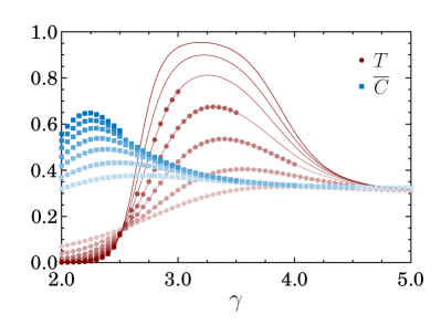
The local clustering coefficient Ci=ni/nisubscript𝐶𝑖superscriptsubscript𝑛𝑖superscriptsubscript𝑛𝑖C_{i}=n_{i}^{\triangle}/n_{i}^{\wedge} is the ratio between the number of triangles connected to and the number of triads centered on node i𝑖i. The mean local clustering C¯=1/NiCi¯𝐶1𝑁subscript𝑖subscript𝐶𝑖{\overline{C}}=1/N\sum_{i}C_{i} is another global measure of the network structure. While in general T𝑇T and C¯¯𝐶\overline{C} do not coincide, they both tend to zero with the system size in locally treelike random network models [40, 41]. We measure numerically C¯¯𝐶{\overline{C}} in STC networks obtained from ER backbones, and we compare it with transitivity in FIG. 3. Despite some quantitative difference, the two quantities exhibit the same qualitative behavior in this case. A different scenario occurs in STC networks obtained from PL backbones. We measure numerically C¯¯𝐶{\overline{C}} for various values of γ𝛾\gamma and report the results in FIG. 6. It turns out that the mean clustering coefficient does not exhibit the transitions occurring for transitivity in the large-N𝑁N limit. Instead C¯¯𝐶\overline{C} changes smoothly with γ𝛾\gamma and also displays much smaller finite size effects. We can get some physical intuition of this qualitative difference between C¯¯𝐶\overline{C} and T𝑇T by expressing T𝑇T as a weighted average of the local clustering coefficient Cisubscript𝐶𝑖C_{i}[38]

T=3×13iniini=iniCiini.𝑇313subscript𝑖superscriptsubscript𝑛𝑖subscript𝑖superscriptsubscript𝑛𝑖subscript𝑖superscriptsubscript𝑛𝑖subscript𝐶𝑖subscript𝑖superscriptsubscript𝑛𝑖T=\frac{3\times\frac{1}{3}\sum_{i}n_{i}^{\triangle}}{\sum_{i}n_{i}^{\wedge}}=\frac{\sum_{i}n_{i}^{\wedge}C_{i}}{\sum_{i}n_{i}^{\wedge}}. (10)

For PL backbones with γ<4𝛾4\gamma<4 both the numerator and the denominator in Eq. (10) diverge, as we already observed in Eq. (9). For γ<5/2𝛾52\gamma<5/2, however, the divergence of the numerator is tamed by the factor Cisubscript𝐶𝑖C_{i}, and the result is a vanishing transitivity.
Refer to caption
Figure 6: Transitivity T𝑇T and mean local clustering coefficient C¯¯𝐶{\overline{C}} as a function of γ𝛾\gamma for PL backbones, for different values of kcsubscript𝑘𝑐k_{c}, with f=1𝑓1f=1 and kmin=3subscript𝑘min3k_{\textrm{min}}=3. Values of kcsubscript𝑘𝑐k_{c}: 100,300,1000,3000,10000,30000,100000100300100030001000030000100000100,300,1000,3000,10000,30000,100000. Darker colors correspond to bigger values of kcsubscript𝑘𝑐k_{c}. The solid red lines are the exact transitivity values, obtained by numerically evaluating Eq. (7). Markers correspond to simulation results. In order to correctly sample a PL degree distribution, for a given kcsubscript𝑘𝑐k_{c}, the number of nodes in the sample must fulfil N>kcγ1𝑁superscriptsubscript𝑘𝑐𝛾1N>k_{c}^{\gamma-1}. This criterion makes simulations involving high kcsubscript𝑘𝑐k_{c} and γ𝛾\gamma values computationally infeasible. For γ𝛾\gamma\to\infty the PL backbone network converges to a random regular network of degree kminsubscript𝑘mink_{\textrm{min}}. In this limit, since all degrees are the same, both T𝑇T and C¯¯𝐶\overline{C} are easily evaluated when f=1𝑓1f=1: limγT=limγC¯=1/kminsubscript𝛾𝑇subscript𝛾¯𝐶1subscript𝑘min\lim_{\gamma\to\infty}T=\lim_{\gamma\to\infty}\overline{C}=1/k_{\textrm{min}}. This limit is already clearly observed for γ5𝛾5\gamma\approx 5.

V Higher-order motifs

The complex structure of 𝒢fsubscript𝒢𝑓\mathcal{G}_{f} is not limited to a large number of triangles. Higher-order motifs, such as overlapping triangles, loops and cliques, are also naturally created by the STC mechanism. In this Section, by exploiting the treelike structure of 𝒢0subscript𝒢0\mathcal{G}_{0} we derive exact expressions for the number of some higher-order motifs in 𝒢fsubscript𝒢𝑓\mathcal{G}_{f}.

V.1 Diamonds and 444-loops

A ubiquitous feature of real social networks is not only their high clustering, but that triangles tend to overlap, significantly altering the dynamics in various types of processes occurring on these networks. The frequency of triangle overlaps both in the STC model and in real-world networks may be measured in various ways. Here we focus on diamonds (two triangles that share a link, that we call the “center” of the motif) and 444-loops (loops of length 4).

V.1.1 Average number of diamonds

The easiest way to compute the expected number of diamonds in 𝒢fsubscript𝒢𝑓\mathcal{G}_{f}, denoted by Nsubscript𝑁N_{\leavevmode\hbox to4.4pt{\vbox to4.4pt{\pgfpicture\makeatletter\hbox{\hskip 0.2pt\lower-0.2pt\hbox to0.0pt{\pgfsys@beginscope\pgfsys@invoke{ }\definecolor{pgfstrokecolor}{rgb}{0,0,0}\pgfsys@color@rgb@stroke{0}{0}{0}\pgfsys@invoke{ }\pgfsys@color@rgb@fill{0}{0}{0}\pgfsys@invoke{ }\pgfsys@setlinewidth{0.4pt}\pgfsys@invoke{ }\nullfont\hbox to0.0pt{\pgfsys@beginscope\pgfsys@invoke{ }{{}{{}}{} {}{{}}{}{}{}{}{{}}{}{}\pgfsys@moveto{0.0pt}{0.0pt}\pgfsys@moveto{0.0pt}{0.0pt}\pgfsys@lineto{0.0pt}{4.0pt}\pgfsys@lineto{4.0pt}{4.0pt}\pgfsys@lineto{4.0pt}{0.0pt}\pgfsys@closepath\pgfsys@moveto{4.0pt}{4.0pt}\pgfsys@stroke\pgfsys@invoke{ } {}{{}}{} {}{}{}\pgfsys@moveto{0.0pt}{0.0pt}\pgfsys@lineto{4.0pt}{4.0pt}\pgfsys@stroke\pgfsys@invoke{ } } \pgfsys@invoke{\lxSVG@closescope }\pgfsys@endscope{}{}{}\hss}\pgfsys@discardpath\pgfsys@invoke{\lxSVG@closescope }\pgfsys@endscope\hss}}\lxSVG@closescope\endpgfpicture}}}, is to write

N=N(old)+N(new),subscript𝑁superscriptsubscript𝑁oldsuperscriptsubscript𝑁newN_{\leavevmode\hbox to4.4pt{\vbox to4.4pt{\pgfpicture\makeatletter\hbox{\hskip 0.2pt\lower-0.2pt\hbox to0.0pt{\pgfsys@beginscope\pgfsys@invoke{ }\definecolor{pgfstrokecolor}{rgb}{0,0,0}\pgfsys@color@rgb@stroke{0}{0}{0}\pgfsys@invoke{ }\pgfsys@color@rgb@fill{0}{0}{0}\pgfsys@invoke{ }\pgfsys@setlinewidth{0.4pt}\pgfsys@invoke{ }\nullfont\hbox to0.0pt{\pgfsys@beginscope\pgfsys@invoke{ }{{}{{}}{} {}{{}}{}{}{}{}{{}}{}{}\pgfsys@moveto{0.0pt}{0.0pt}\pgfsys@moveto{0.0pt}{0.0pt}\pgfsys@lineto{0.0pt}{4.0pt}\pgfsys@lineto{4.0pt}{4.0pt}\pgfsys@lineto{4.0pt}{0.0pt}\pgfsys@closepath\pgfsys@moveto{4.0pt}{4.0pt}\pgfsys@stroke\pgfsys@invoke{ } {}{{}}{} {}{}{}\pgfsys@moveto{0.0pt}{0.0pt}\pgfsys@lineto{4.0pt}{4.0pt}\pgfsys@stroke\pgfsys@invoke{ } } \pgfsys@invoke{\lxSVG@closescope }\pgfsys@endscope{}{}{}\hss}\pgfsys@discardpath\pgfsys@invoke{\lxSVG@closescope }\pgfsys@endscope\hss}}\lxSVG@closescope\endpgfpicture}}}=N_{\leavevmode\hbox to4.4pt{\vbox to4.4pt{\pgfpicture\makeatletter\hbox{\hskip 0.2pt\lower-0.2pt\hbox to0.0pt{\pgfsys@beginscope\pgfsys@invoke{ }\definecolor{pgfstrokecolor}{rgb}{0,0,0}\pgfsys@color@rgb@stroke{0}{0}{0}\pgfsys@invoke{ }\pgfsys@color@rgb@fill{0}{0}{0}\pgfsys@invoke{ }\pgfsys@setlinewidth{0.4pt}\pgfsys@invoke{ }\nullfont\hbox to0.0pt{\pgfsys@beginscope\pgfsys@invoke{ }{{}{{}}{} {}{{}}{}{}{}{}{{}}{}{}\pgfsys@moveto{0.0pt}{0.0pt}\pgfsys@moveto{0.0pt}{0.0pt}\pgfsys@lineto{0.0pt}{4.0pt}\pgfsys@lineto{4.0pt}{4.0pt}\pgfsys@lineto{4.0pt}{0.0pt}\pgfsys@closepath\pgfsys@moveto{4.0pt}{4.0pt}\pgfsys@stroke\pgfsys@invoke{ } {}{{}}{} {}{}{}\pgfsys@moveto{0.0pt}{0.0pt}\pgfsys@lineto{4.0pt}{4.0pt}\pgfsys@stroke\pgfsys@invoke{ } } \pgfsys@invoke{\lxSVG@closescope }\pgfsys@endscope{}{}{}\hss}\pgfsys@discardpath\pgfsys@invoke{\lxSVG@closescope }\pgfsys@endscope\hss}}\lxSVG@closescope\endpgfpicture}}}^{(\text{old})}+N_{\leavevmode\hbox to4.4pt{\vbox to4.4pt{\pgfpicture\makeatletter\hbox{\hskip 0.2pt\lower-0.2pt\hbox to0.0pt{\pgfsys@beginscope\pgfsys@invoke{ }\definecolor{pgfstrokecolor}{rgb}{0,0,0}\pgfsys@color@rgb@stroke{0}{0}{0}\pgfsys@invoke{ }\pgfsys@color@rgb@fill{0}{0}{0}\pgfsys@invoke{ }\pgfsys@setlinewidth{0.4pt}\pgfsys@invoke{ }\nullfont\hbox to0.0pt{\pgfsys@beginscope\pgfsys@invoke{ }{{}{{}}{} {}{{}}{}{}{}{}{{}}{}{}\pgfsys@moveto{0.0pt}{0.0pt}\pgfsys@moveto{0.0pt}{0.0pt}\pgfsys@lineto{0.0pt}{4.0pt}\pgfsys@lineto{4.0pt}{4.0pt}\pgfsys@lineto{4.0pt}{0.0pt}\pgfsys@closepath\pgfsys@moveto{4.0pt}{4.0pt}\pgfsys@stroke\pgfsys@invoke{ } {}{{}}{} {}{}{}\pgfsys@moveto{0.0pt}{0.0pt}\pgfsys@lineto{4.0pt}{4.0pt}\pgfsys@stroke\pgfsys@invoke{ } } \pgfsys@invoke{\lxSVG@closescope }\pgfsys@endscope{}{}{}\hss}\pgfsys@discardpath\pgfsys@invoke{\lxSVG@closescope }\pgfsys@endscope\hss}}\lxSVG@closescope\endpgfpicture}}}^{(\text{new})},

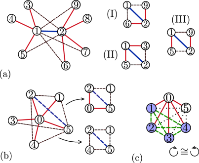
where N(old)superscriptsubscript𝑁oldN_{\leavevmode\hbox to4.4pt{\vbox to4.4pt{\pgfpicture\makeatletter\hbox{\hskip 0.2pt\lower-0.2pt\hbox to0.0pt{\pgfsys@beginscope\pgfsys@invoke{ }\definecolor{pgfstrokecolor}{rgb}{0,0,0}\pgfsys@color@rgb@stroke{0}{0}{0}\pgfsys@invoke{ }\pgfsys@color@rgb@fill{0}{0}{0}\pgfsys@invoke{ }\pgfsys@setlinewidth{0.4pt}\pgfsys@invoke{ }\nullfont\hbox to0.0pt{\pgfsys@beginscope\pgfsys@invoke{ }{{}{{}}{} {}{{}}{}{}{}{}{{}}{}{}\pgfsys@moveto{0.0pt}{0.0pt}\pgfsys@moveto{0.0pt}{0.0pt}\pgfsys@lineto{0.0pt}{4.0pt}\pgfsys@lineto{4.0pt}{4.0pt}\pgfsys@lineto{4.0pt}{0.0pt}\pgfsys@closepath\pgfsys@moveto{4.0pt}{4.0pt}\pgfsys@stroke\pgfsys@invoke{ } {}{{}}{} {}{}{}\pgfsys@moveto{0.0pt}{0.0pt}\pgfsys@lineto{4.0pt}{4.0pt}\pgfsys@stroke\pgfsys@invoke{ } } \pgfsys@invoke{\lxSVG@closescope }\pgfsys@endscope{}{}{}\hss}\pgfsys@discardpath\pgfsys@invoke{\lxSVG@closescope }\pgfsys@endscope\hss}}\lxSVG@closescope\endpgfpicture}}}^{(\text{old})} and N(new)superscriptsubscript𝑁newN_{\leavevmode\hbox to4.4pt{\vbox to4.4pt{\pgfpicture\makeatletter\hbox{\hskip 0.2pt\lower-0.2pt\hbox to0.0pt{\pgfsys@beginscope\pgfsys@invoke{ }\definecolor{pgfstrokecolor}{rgb}{0,0,0}\pgfsys@color@rgb@stroke{0}{0}{0}\pgfsys@invoke{ }\pgfsys@color@rgb@fill{0}{0}{0}\pgfsys@invoke{ }\pgfsys@setlinewidth{0.4pt}\pgfsys@invoke{ }\nullfont\hbox to0.0pt{\pgfsys@beginscope\pgfsys@invoke{ }{{}{{}}{} {}{{}}{}{}{}{}{{}}{}{}\pgfsys@moveto{0.0pt}{0.0pt}\pgfsys@moveto{0.0pt}{0.0pt}\pgfsys@lineto{0.0pt}{4.0pt}\pgfsys@lineto{4.0pt}{4.0pt}\pgfsys@lineto{4.0pt}{0.0pt}\pgfsys@closepath\pgfsys@moveto{4.0pt}{4.0pt}\pgfsys@stroke\pgfsys@invoke{ } {}{{}}{} {}{}{}\pgfsys@moveto{0.0pt}{0.0pt}\pgfsys@lineto{4.0pt}{4.0pt}\pgfsys@stroke\pgfsys@invoke{ } } \pgfsys@invoke{\lxSVG@closescope }\pgfsys@endscope{}{}{}\hss}\pgfsys@discardpath\pgfsys@invoke{\lxSVG@closescope }\pgfsys@endscope\hss}}\lxSVG@closescope\endpgfpicture}}}^{(\text{new})} are the number of diamonds centered on old links, i.e. links that are in 0subscript0\mathcal{E}_{0}, and on new links, i.e. links that are in f0subscript𝑓subscript0\mathcal{E}_{f}\setminus\mathcal{E}_{0}, respectively. Consider an old edge (as (1,2)12(1,2) in FIG. 7) with end nodes i𝑖i and j𝑗j. Denoting by nijsubscript𝑛𝑖𝑗n_{i\to\partial j} the number of new links created on average by the STC mechanism between node i𝑖i and jssuperscript𝑗𝑠j^{\prime}s neighbors, we can distinguish three topologically different diamonds centered on the old link (i,j)𝑖𝑗(i,j) (see FIG. 7(a)):

  1. I.

    the ones in which we take two among j𝑗j’s neighbors which have become also i𝑖i’s neighbors. There are nij(nij1)/2subscript𝑛𝑖𝑗subscript𝑛𝑖𝑗12n_{i\to\partial j}(n_{i\to\partial j}-1)/2 of them;

  2. II.

    the ones in which we take two among i𝑖i’s neighbors which have become also j𝑗j’s neighbors. There are nji(nji1)/2subscript𝑛𝑗𝑖subscript𝑛𝑗𝑖12n_{j\to\partial i}(n_{j\to\partial i}-1)/2 of them;

  3. III.

    the ones in which we consider one neighbor of node i𝑖i and one neighbor of node j𝑗j. There are nijnjisubscript𝑛𝑖𝑗subscript𝑛𝑗𝑖n_{i\to\partial j}n_{j\to\partial i} of them.

Summing these contributions and averaging over pksubscript𝑝𝑘p_{k} we get

N(old)superscriptsubscript𝑁old\displaystyle N_{\leavevmode\hbox to4.4pt{\vbox to4.4pt{\pgfpicture\makeatletter\hbox{\hskip 0.2pt\lower-0.2pt\hbox to0.0pt{\pgfsys@beginscope\pgfsys@invoke{ }\definecolor{pgfstrokecolor}{rgb}{0,0,0}\pgfsys@color@rgb@stroke{0}{0}{0}\pgfsys@invoke{ }\pgfsys@color@rgb@fill{0}{0}{0}\pgfsys@invoke{ }\pgfsys@setlinewidth{0.4pt}\pgfsys@invoke{ }\nullfont\hbox to0.0pt{\pgfsys@beginscope\pgfsys@invoke{ }{{}{{}}{} {}{{}}{}{}{}{}{{}}{}{}\pgfsys@moveto{0.0pt}{0.0pt}\pgfsys@moveto{0.0pt}{0.0pt}\pgfsys@lineto{0.0pt}{4.0pt}\pgfsys@lineto{4.0pt}{4.0pt}\pgfsys@lineto{4.0pt}{0.0pt}\pgfsys@closepath\pgfsys@moveto{4.0pt}{4.0pt}\pgfsys@stroke\pgfsys@invoke{ } {}{{}}{} {}{}{}\pgfsys@moveto{0.0pt}{0.0pt}\pgfsys@lineto{4.0pt}{4.0pt}\pgfsys@stroke\pgfsys@invoke{ } } \pgfsys@invoke{\lxSVG@closescope }\pgfsys@endscope{}{}{}\hss}\pgfsys@discardpath\pgfsys@invoke{\lxSVG@closescope }\pgfsys@endscope\hss}}\lxSVG@closescope\endpgfpicture}}}^{(\text{old})} =Nk4ηij(ηij1)absent𝑁delimited-⟨⟩𝑘4delimited-⟨⟩subscript𝜂𝑖𝑗subscript𝜂𝑖𝑗1\displaystyle=\frac{N\langle k\rangle}{4}\langle\eta_{ij}(\eta_{ij}-1)\rangle (11)

where ηij=nij+njisubscript𝜂𝑖𝑗subscript𝑛𝑖𝑗subscript𝑛𝑗𝑖\eta_{ij}=n_{i\to\partial j}+n_{j\to\partial i}. Using the fact that nijsubscript𝑛𝑖𝑗n_{i\to\partial j} and njisubscript𝑛𝑗𝑖n_{j\to\partial i} are i.i.d. random variables whose probability generating function is given by g1(1f+fz)subscript𝑔11𝑓𝑓𝑧g_{1}(1-f+fz) (see Sec. III), it follows that the generating function of the probability distribution of the variables ηijsubscript𝜂𝑖𝑗\eta_{ij} is H(z)=[g1(1f+fz)]2𝐻𝑧superscriptdelimited-[]subscript𝑔11𝑓𝑓𝑧2H(z)=\left[g_{1}(1-f+fz)\right]^{2}. Hence we have

N(old)superscriptsubscript𝑁old\displaystyle N_{\leavevmode\hbox to4.4pt{\vbox to4.4pt{\pgfpicture\makeatletter\hbox{\hskip 0.2pt\lower-0.2pt\hbox to0.0pt{\pgfsys@beginscope\pgfsys@invoke{ }\definecolor{pgfstrokecolor}{rgb}{0,0,0}\pgfsys@color@rgb@stroke{0}{0}{0}\pgfsys@invoke{ }\pgfsys@color@rgb@fill{0}{0}{0}\pgfsys@invoke{ }\pgfsys@setlinewidth{0.4pt}\pgfsys@invoke{ }\nullfont\hbox to0.0pt{\pgfsys@beginscope\pgfsys@invoke{ }{{}{{}}{} {}{{}}{}{}{}{}{{}}{}{}\pgfsys@moveto{0.0pt}{0.0pt}\pgfsys@moveto{0.0pt}{0.0pt}\pgfsys@lineto{0.0pt}{4.0pt}\pgfsys@lineto{4.0pt}{4.0pt}\pgfsys@lineto{4.0pt}{0.0pt}\pgfsys@closepath\pgfsys@moveto{4.0pt}{4.0pt}\pgfsys@stroke\pgfsys@invoke{ } {}{{}}{} {}{}{}\pgfsys@moveto{0.0pt}{0.0pt}\pgfsys@lineto{4.0pt}{4.0pt}\pgfsys@stroke\pgfsys@invoke{ } } \pgfsys@invoke{\lxSVG@closescope }\pgfsys@endscope{}{}{}\hss}\pgfsys@discardpath\pgfsys@invoke{\lxSVG@closescope }\pgfsys@endscope\hss}}\lxSVG@closescope\endpgfpicture}}}^{(\text{old})} =Nk4H′′(1)=Nf22[μ3+μ22/μ1].absent𝑁delimited-⟨⟩𝑘4superscript𝐻′′1𝑁superscript𝑓22delimited-[]subscript𝜇3superscriptsubscript𝜇22subscript𝜇1\displaystyle=\frac{N\langle k\rangle}{4}H^{\prime\prime}(1)=\frac{Nf^{2}}{2}\left[\mu_{3}+\mu_{2}^{2}/\mu_{1}\right]. (12)

Now consider a node of degree k𝑘k in 𝒢0subscript𝒢0\mathcal{G}_{0}, and a new edge (a,b)𝑎𝑏(a,b) created among its neighbors. A diamond centered on this edge can be formed only because of the creation of new links among the other (k2)𝑘2(k-2) neighbors of the node, since nodes a𝑎a and b𝑏b are second neighbors in the original network. There are on average fk(k1)/2𝑓𝑘𝑘12fk(k-1)/2 new links such as (a,b)𝑎𝑏(a,b). This link can be the center either of a diamond with 222 old links and 222 new links on the perimeter, or can be the center of a diamond with 444 new links on the perimeter (see FIG. 7(b)). First we consider the diamonds with two old links on the perimeter. Fixed the link (a,b)𝑎𝑏(a,b), there are k2𝑘2k-2 ways of choosing the third node, and hence we have f3k(k1)(k2)/2superscript𝑓3𝑘𝑘1𝑘22f^{3}k(k-1)(k-2)/2 distinct motifs. In the other case, we can pick the two other nodes to complete the diamond by choosing among the remaining (k2)(k3)𝑘2𝑘3(k-2)(k-3) nodes, and we can do this in (k2)(k3)/2𝑘2𝑘32(k-2)(k-3)/2 distinct ways. The total number of such motifs is f5k(k1)(k2)(k3)/4superscript𝑓5𝑘𝑘1𝑘2𝑘34f^{5}k(k-1)(k-2)(k-3)/4. Averaging over pksubscript𝑝𝑘p_{k} we get

N(new)subscriptsuperscript𝑁new\displaystyle N^{(\text{new})}_{\leavevmode\hbox to4.4pt{\vbox to4.4pt{\pgfpicture\makeatletter\hbox{\hskip 0.2pt\lower-0.2pt\hbox to0.0pt{\pgfsys@beginscope\pgfsys@invoke{ }\definecolor{pgfstrokecolor}{rgb}{0,0,0}\pgfsys@color@rgb@stroke{0}{0}{0}\pgfsys@invoke{ }\pgfsys@color@rgb@fill{0}{0}{0}\pgfsys@invoke{ }\pgfsys@setlinewidth{0.4pt}\pgfsys@invoke{ }\nullfont\hbox to0.0pt{\pgfsys@beginscope\pgfsys@invoke{ }{{}{{}}{} {}{{}}{}{}{}{}{{}}{}{}\pgfsys@moveto{0.0pt}{0.0pt}\pgfsys@moveto{0.0pt}{0.0pt}\pgfsys@lineto{0.0pt}{4.0pt}\pgfsys@lineto{4.0pt}{4.0pt}\pgfsys@lineto{4.0pt}{0.0pt}\pgfsys@closepath\pgfsys@moveto{4.0pt}{4.0pt}\pgfsys@stroke\pgfsys@invoke{ } {}{{}}{} {}{}{}\pgfsys@moveto{0.0pt}{0.0pt}\pgfsys@lineto{4.0pt}{4.0pt}\pgfsys@stroke\pgfsys@invoke{ } } \pgfsys@invoke{\lxSVG@closescope }\pgfsys@endscope{}{}{}\hss}\pgfsys@discardpath\pgfsys@invoke{\lxSVG@closescope }\pgfsys@endscope\hss}}\lxSVG@closescope\endpgfpicture}}} =N[f3μ32+f5μ44].absent𝑁delimited-[]superscript𝑓3subscript𝜇32superscript𝑓5subscript𝜇44\displaystyle=N\left[f^{3}\frac{\mu_{3}}{2}+f^{5}\frac{\mu_{4}}{4}\right]. (13)

Summing up we finally have

N=Nf24[2μ22/μ1+2(1+f)μ3+f3μ4].subscript𝑁𝑁superscript𝑓24delimited-[]2superscriptsubscript𝜇22subscript𝜇121𝑓subscript𝜇3superscript𝑓3subscript𝜇4\displaystyle N_{\leavevmode\hbox to4.4pt{\vbox to4.4pt{\pgfpicture\makeatletter\hbox{\hskip 0.2pt\lower-0.2pt\hbox to0.0pt{\pgfsys@beginscope\pgfsys@invoke{ }\definecolor{pgfstrokecolor}{rgb}{0,0,0}\pgfsys@color@rgb@stroke{0}{0}{0}\pgfsys@invoke{ }\pgfsys@color@rgb@fill{0}{0}{0}\pgfsys@invoke{ }\pgfsys@setlinewidth{0.4pt}\pgfsys@invoke{ }\nullfont\hbox to0.0pt{\pgfsys@beginscope\pgfsys@invoke{ }{{}{{}}{} {}{{}}{}{}{}{}{{}}{}{}\pgfsys@moveto{0.0pt}{0.0pt}\pgfsys@moveto{0.0pt}{0.0pt}\pgfsys@lineto{0.0pt}{4.0pt}\pgfsys@lineto{4.0pt}{4.0pt}\pgfsys@lineto{4.0pt}{0.0pt}\pgfsys@closepath\pgfsys@moveto{4.0pt}{4.0pt}\pgfsys@stroke\pgfsys@invoke{ } {}{{}}{} {}{}{}\pgfsys@moveto{0.0pt}{0.0pt}\pgfsys@lineto{4.0pt}{4.0pt}\pgfsys@stroke\pgfsys@invoke{ } } \pgfsys@invoke{\lxSVG@closescope }\pgfsys@endscope{}{}{}\hss}\pgfsys@discardpath\pgfsys@invoke{\lxSVG@closescope }\pgfsys@endscope\hss}}\lxSVG@closescope\endpgfpicture}}}=\frac{Nf^{2}}{4}\left[2\mu_{2}^{2}/\mu_{1}+2(1+f)\mu_{3}+f^{3}\mu_{4}\right]. (14)

V.1.2 Average number of 444-loops

To compute the average number of 444-loops, a simple observation is crucial: any 4limit-from44-loop must contain either zero or two old links, by construction. The average number of 444-loops with two old edges, denoted by N(2)subscriptsuperscript𝑁2N^{(2)}_{\leavevmode\hbox to4.4pt{\vbox to4.4pt{\pgfpicture\makeatletter\hbox{\hskip 0.2pt\lower-0.2pt\hbox to0.0pt{\pgfsys@beginscope\pgfsys@invoke{ }\definecolor{pgfstrokecolor}{rgb}{0,0,0}\pgfsys@color@rgb@stroke{0}{0}{0}\pgfsys@invoke{ }\pgfsys@color@rgb@fill{0}{0}{0}\pgfsys@invoke{ }\pgfsys@setlinewidth{0.4pt}\pgfsys@invoke{ }\nullfont\hbox to0.0pt{\pgfsys@beginscope\pgfsys@invoke{ }{{}{{}}{} {}{{}}{}{}{}{}{{}}{}{}\pgfsys@moveto{0.0pt}{0.0pt}\pgfsys@moveto{0.0pt}{0.0pt}\pgfsys@lineto{0.0pt}{4.0pt}\pgfsys@lineto{4.0pt}{4.0pt}\pgfsys@lineto{4.0pt}{0.0pt}\pgfsys@closepath\pgfsys@moveto{4.0pt}{4.0pt}\pgfsys@stroke\pgfsys@invoke{ } } \pgfsys@invoke{\lxSVG@closescope }\pgfsys@endscope{}{}{}\hss}\pgfsys@discardpath\pgfsys@invoke{\lxSVG@closescope }\pgfsys@endscope\hss}}\lxSVG@closescope\endpgfpicture}}}, is the same as the number of diamonds centered on old links given in Eq. (12), see FIG. 7. The number of 444-loops with zero old links, denoted N(0)subscriptsuperscript𝑁0N^{(0)}_{\leavevmode\hbox to4.4pt{\vbox to4.4pt{\pgfpicture\makeatletter\hbox{\hskip 0.2pt\lower-0.2pt\hbox to0.0pt{\pgfsys@beginscope\pgfsys@invoke{ }\definecolor{pgfstrokecolor}{rgb}{0,0,0}\pgfsys@color@rgb@stroke{0}{0}{0}\pgfsys@invoke{ }\pgfsys@color@rgb@fill{0}{0}{0}\pgfsys@invoke{ }\pgfsys@setlinewidth{0.4pt}\pgfsys@invoke{ }\nullfont\hbox to0.0pt{\pgfsys@beginscope\pgfsys@invoke{ }{{}{{}}{} {}{{}}{}{}{}{}{{}}{}{}\pgfsys@moveto{0.0pt}{0.0pt}\pgfsys@moveto{0.0pt}{0.0pt}\pgfsys@lineto{0.0pt}{4.0pt}\pgfsys@lineto{4.0pt}{4.0pt}\pgfsys@lineto{4.0pt}{0.0pt}\pgfsys@closepath\pgfsys@moveto{4.0pt}{4.0pt}\pgfsys@stroke\pgfsys@invoke{ } } \pgfsys@invoke{\lxSVG@closescope }\pgfsys@endscope{}{}{}\hss}\pgfsys@discardpath\pgfsys@invoke{\lxSVG@closescope }\pgfsys@endscope\hss}}\lxSVG@closescope\endpgfpicture}}}, is instead simply given by (see FIG. 7(c))

N(0)=Nf4μ48,subscriptsuperscript𝑁0𝑁superscript𝑓4subscript𝜇48\displaystyle N^{(0)}_{\leavevmode\hbox to4.4pt{\vbox to4.4pt{\pgfpicture\makeatletter\hbox{\hskip 0.2pt\lower-0.2pt\hbox to0.0pt{\pgfsys@beginscope\pgfsys@invoke{ }\definecolor{pgfstrokecolor}{rgb}{0,0,0}\pgfsys@color@rgb@stroke{0}{0}{0}\pgfsys@invoke{ }\pgfsys@color@rgb@fill{0}{0}{0}\pgfsys@invoke{ }\pgfsys@setlinewidth{0.4pt}\pgfsys@invoke{ }\nullfont\hbox to0.0pt{\pgfsys@beginscope\pgfsys@invoke{ }{{}{{}}{} {}{{}}{}{}{}{}{{}}{}{}\pgfsys@moveto{0.0pt}{0.0pt}\pgfsys@moveto{0.0pt}{0.0pt}\pgfsys@lineto{0.0pt}{4.0pt}\pgfsys@lineto{4.0pt}{4.0pt}\pgfsys@lineto{4.0pt}{0.0pt}\pgfsys@closepath\pgfsys@moveto{4.0pt}{4.0pt}\pgfsys@stroke\pgfsys@invoke{ } } \pgfsys@invoke{\lxSVG@closescope }\pgfsys@endscope{}{}{}\hss}\pgfsys@discardpath\pgfsys@invoke{\lxSVG@closescope }\pgfsys@endscope\hss}}\lxSVG@closescope\endpgfpicture}}}=\frac{Nf^{4}\mu_{4}}{8}, (15)

since we have k(k1)(k2)(k3)𝑘𝑘1𝑘2𝑘3k(k-1)(k-2)(k-3) ways of picking 444 nodes among the neighbors of a random node of original degree k𝑘k, and in a loop the order in which we choose the nodes matters: we have 444 possible ways of starting the loop, and 222 possible choices of orientation, which gives the factor 1/8181/8. Putting these two contributions together we get

N=Nf28[4μ3+4μ22/μ1+f2μ4].subscript𝑁𝑁superscript𝑓28delimited-[]4subscript𝜇34superscriptsubscript𝜇22subscript𝜇1superscript𝑓2subscript𝜇4\displaystyle N_{\leavevmode\hbox to4.4pt{\vbox to4.4pt{\pgfpicture\makeatletter\hbox{\hskip 0.2pt\lower-0.2pt\hbox to0.0pt{\pgfsys@beginscope\pgfsys@invoke{ }\definecolor{pgfstrokecolor}{rgb}{0,0,0}\pgfsys@color@rgb@stroke{0}{0}{0}\pgfsys@invoke{ }\pgfsys@color@rgb@fill{0}{0}{0}\pgfsys@invoke{ }\pgfsys@setlinewidth{0.4pt}\pgfsys@invoke{ }\nullfont\hbox to0.0pt{\pgfsys@beginscope\pgfsys@invoke{ }{{}{{}}{} {}{{}}{}{}{}{}{{}}{}{}\pgfsys@moveto{0.0pt}{0.0pt}\pgfsys@moveto{0.0pt}{0.0pt}\pgfsys@lineto{0.0pt}{4.0pt}\pgfsys@lineto{4.0pt}{4.0pt}\pgfsys@lineto{4.0pt}{0.0pt}\pgfsys@closepath\pgfsys@moveto{4.0pt}{4.0pt}\pgfsys@stroke\pgfsys@invoke{ } } \pgfsys@invoke{\lxSVG@closescope }\pgfsys@endscope{}{}{}\hss}\pgfsys@discardpath\pgfsys@invoke{\lxSVG@closescope }\pgfsys@endscope\hss}}\lxSVG@closescope\endpgfpicture}}}=\frac{Nf^{2}}{8}\left[4\mu_{3}+4\mu_{2}^{2}/\mu_{1}+f^{2}\mu_{4}\right]. (16)

V.1.3 444-loops made of overlapping triangles

It is useful to define the quantity444Only for f>0𝑓0f>0, since for f=0𝑓0f=0 both the numerator and the denominator are zero.

R=N2N,subscript𝑅subscript𝑁2subscript𝑁R_{\operatorname{\mkern 1.0mu\leavevmode\hbox to4.4pt{\vbox to4.4pt{\pgfpicture\makeatletter\hbox{\hskip 0.2pt\lower-0.2pt\hbox to0.0pt{\pgfsys@beginscope\pgfsys@invoke{ }\definecolor{pgfstrokecolor}{rgb}{0,0,0}\pgfsys@color@rgb@stroke{0}{0}{0}\pgfsys@invoke{ }\pgfsys@color@rgb@fill{0}{0}{0}\pgfsys@invoke{ }\pgfsys@setlinewidth{0.4pt}\pgfsys@invoke{ }\nullfont\hbox to0.0pt{\pgfsys@beginscope\pgfsys@invoke{ }{{}{{}}{} {}{{}}{}{}{}{}{{}}{}{}\pgfsys@moveto{0.0pt}{0.0pt}\pgfsys@moveto{0.0pt}{0.0pt}\pgfsys@lineto{0.0pt}{4.0pt}\pgfsys@lineto{4.0pt}{4.0pt}\pgfsys@lineto{4.0pt}{0.0pt}\pgfsys@closepath\pgfsys@moveto{4.0pt}{4.0pt}\pgfsys@stroke\pgfsys@invoke{ } {}{{}}{} {}{}{}\pgfsys@moveto{0.0pt}{0.0pt}\pgfsys@lineto{4.0pt}{4.0pt}\pgfsys@stroke\pgfsys@invoke{ } } \pgfsys@invoke{\lxSVG@closescope }\pgfsys@endscope{}{}{}\hss}\pgfsys@discardpath\pgfsys@invoke{\lxSVG@closescope }\pgfsys@endscope\hss}}\lxSVG@closescope\endpgfpicture}}}}=\frac{N_{\leavevmode\hbox to4.4pt{\vbox to4.4pt{\pgfpicture\makeatletter\hbox{\hskip 0.2pt\lower-0.2pt\hbox to0.0pt{\pgfsys@beginscope\pgfsys@invoke{ }\definecolor{pgfstrokecolor}{rgb}{0,0,0}\pgfsys@color@rgb@stroke{0}{0}{0}\pgfsys@invoke{ }\pgfsys@color@rgb@fill{0}{0}{0}\pgfsys@invoke{ }\pgfsys@setlinewidth{0.4pt}\pgfsys@invoke{ }\nullfont\hbox to0.0pt{\pgfsys@beginscope\pgfsys@invoke{ }{{}{{}}{} {}{{}}{}{}{}{}{{}}{}{}\pgfsys@moveto{0.0pt}{0.0pt}\pgfsys@moveto{0.0pt}{0.0pt}\pgfsys@lineto{0.0pt}{4.0pt}\pgfsys@lineto{4.0pt}{4.0pt}\pgfsys@lineto{4.0pt}{0.0pt}\pgfsys@closepath\pgfsys@moveto{4.0pt}{4.0pt}\pgfsys@stroke\pgfsys@invoke{ } {}{{}}{} {}{}{}\pgfsys@moveto{0.0pt}{0.0pt}\pgfsys@lineto{4.0pt}{4.0pt}\pgfsys@stroke\pgfsys@invoke{ } } \pgfsys@invoke{\lxSVG@closescope }\pgfsys@endscope{}{}{}\hss}\pgfsys@discardpath\pgfsys@invoke{\lxSVG@closescope }\pgfsys@endscope\hss}}\lxSVG@closescope\endpgfpicture}}}}{2N_{\leavevmode\hbox to4.4pt{\vbox to4.4pt{\pgfpicture\makeatletter\hbox{\hskip 0.2pt\lower-0.2pt\hbox to0.0pt{\pgfsys@beginscope\pgfsys@invoke{ }\definecolor{pgfstrokecolor}{rgb}{0,0,0}\pgfsys@color@rgb@stroke{0}{0}{0}\pgfsys@invoke{ }\pgfsys@color@rgb@fill{0}{0}{0}\pgfsys@invoke{ }\pgfsys@setlinewidth{0.4pt}\pgfsys@invoke{ }\nullfont\hbox to0.0pt{\pgfsys@beginscope\pgfsys@invoke{ }{{}{{}}{} {}{{}}{}{}{}{}{{}}{}{}\pgfsys@moveto{0.0pt}{0.0pt}\pgfsys@moveto{0.0pt}{0.0pt}\pgfsys@lineto{0.0pt}{4.0pt}\pgfsys@lineto{4.0pt}{4.0pt}\pgfsys@lineto{4.0pt}{0.0pt}\pgfsys@closepath\pgfsys@moveto{4.0pt}{4.0pt}\pgfsys@stroke\pgfsys@invoke{ } } \pgfsys@invoke{\lxSVG@closescope }\pgfsys@endscope{}{}{}\hss}\pgfsys@discardpath\pgfsys@invoke{\lxSVG@closescope }\pgfsys@endscope\hss}}\lxSVG@closescope\endpgfpicture}}}}, (17)

which provides a measure of how likely 444-loops are to be made of overlapping triangles (diamonds) in 𝒢fsubscript𝒢𝑓\mathcal{G}_{f}. In an arbitrary network, any diamond corresponds to exactly one 444-loop. Also, any 444-loop corresponds to at most two diamonds. Therefore, for any network R[0,1]subscript𝑅01R_{\operatorname{\mkern 1.0mu\leavevmode\hbox to4.4pt{\vbox to4.4pt{\pgfpicture\makeatletter\hbox{\hskip 0.2pt\lower-0.2pt\hbox to0.0pt{\pgfsys@beginscope\pgfsys@invoke{ }\definecolor{pgfstrokecolor}{rgb}{0,0,0}\pgfsys@color@rgb@stroke{0}{0}{0}\pgfsys@invoke{ }\pgfsys@color@rgb@fill{0}{0}{0}\pgfsys@invoke{ }\pgfsys@setlinewidth{0.4pt}\pgfsys@invoke{ }\nullfont\hbox to0.0pt{\pgfsys@beginscope\pgfsys@invoke{ }{{}{{}}{} {}{{}}{}{}{}{}{{}}{}{}\pgfsys@moveto{0.0pt}{0.0pt}\pgfsys@moveto{0.0pt}{0.0pt}\pgfsys@lineto{0.0pt}{4.0pt}\pgfsys@lineto{4.0pt}{4.0pt}\pgfsys@lineto{4.0pt}{0.0pt}\pgfsys@closepath\pgfsys@moveto{4.0pt}{4.0pt}\pgfsys@stroke\pgfsys@invoke{ } {}{{}}{} {}{}{}\pgfsys@moveto{0.0pt}{0.0pt}\pgfsys@lineto{4.0pt}{4.0pt}\pgfsys@stroke\pgfsys@invoke{ } } \pgfsys@invoke{\lxSVG@closescope }\pgfsys@endscope{}{}{}\hss}\pgfsys@discardpath\pgfsys@invoke{\lxSVG@closescope }\pgfsys@endscope\hss}}\lxSVG@closescope\endpgfpicture}}}}\in[0,1]. From Eqs. (14),(16) we get

R=[2μ22/μ1+2(1+f)μ3+f3μ4][4μ3+4μ22/μ1+f2μ4].subscript𝑅delimited-[]2superscriptsubscript𝜇22subscript𝜇121𝑓subscript𝜇3superscript𝑓3subscript𝜇4delimited-[]4subscript𝜇34superscriptsubscript𝜇22subscript𝜇1superscript𝑓2subscript𝜇4R_{\operatorname{\mkern 1.0mu\leavevmode\hbox to4.4pt{\vbox to4.4pt{\pgfpicture\makeatletter\hbox{\hskip 0.2pt\lower-0.2pt\hbox to0.0pt{\pgfsys@beginscope\pgfsys@invoke{ }\definecolor{pgfstrokecolor}{rgb}{0,0,0}\pgfsys@color@rgb@stroke{0}{0}{0}\pgfsys@invoke{ }\pgfsys@color@rgb@fill{0}{0}{0}\pgfsys@invoke{ }\pgfsys@setlinewidth{0.4pt}\pgfsys@invoke{ }\nullfont\hbox to0.0pt{\pgfsys@beginscope\pgfsys@invoke{ }{{}{{}}{} {}{{}}{}{}{}{}{{}}{}{}\pgfsys@moveto{0.0pt}{0.0pt}\pgfsys@moveto{0.0pt}{0.0pt}\pgfsys@lineto{0.0pt}{4.0pt}\pgfsys@lineto{4.0pt}{4.0pt}\pgfsys@lineto{4.0pt}{0.0pt}\pgfsys@closepath\pgfsys@moveto{4.0pt}{4.0pt}\pgfsys@stroke\pgfsys@invoke{ } {}{{}}{} {}{}{}\pgfsys@moveto{0.0pt}{0.0pt}\pgfsys@lineto{4.0pt}{4.0pt}\pgfsys@stroke\pgfsys@invoke{ } } \pgfsys@invoke{\lxSVG@closescope }\pgfsys@endscope{}{}{}\hss}\pgfsys@discardpath\pgfsys@invoke{\lxSVG@closescope }\pgfsys@endscope\hss}}\lxSVG@closescope\endpgfpicture}}}}=\frac{\left[2\mu_{2}^{2}/\mu_{1}+2(1+f)\mu_{3}+f^{3}\mu_{4}\right]}{\left[4\mu_{3}+4\mu_{2}^{2}/\mu_{1}+f^{2}\mu_{4}\right]}. (18)

From this expression, it follows that for PL networks Rfsubscript𝑅𝑓R_{\operatorname{\mkern 1.0mu\leavevmode\hbox to4.4pt{\vbox to4.4pt{\pgfpicture\makeatletter\hbox{\hskip 0.2pt\lower-0.2pt\hbox to0.0pt{\pgfsys@beginscope\pgfsys@invoke{ }\definecolor{pgfstrokecolor}{rgb}{0,0,0}\pgfsys@color@rgb@stroke{0}{0}{0}\pgfsys@invoke{ }\pgfsys@color@rgb@fill{0}{0}{0}\pgfsys@invoke{ }\pgfsys@setlinewidth{0.4pt}\pgfsys@invoke{ }\nullfont\hbox to0.0pt{\pgfsys@beginscope\pgfsys@invoke{ }{{}{{}}{} {}{{}}{}{}{}{}{{}}{}{}\pgfsys@moveto{0.0pt}{0.0pt}\pgfsys@moveto{0.0pt}{0.0pt}\pgfsys@lineto{0.0pt}{4.0pt}\pgfsys@lineto{4.0pt}{4.0pt}\pgfsys@lineto{4.0pt}{0.0pt}\pgfsys@closepath\pgfsys@moveto{4.0pt}{4.0pt}\pgfsys@stroke\pgfsys@invoke{ } {}{{}}{} {}{}{}\pgfsys@moveto{0.0pt}{0.0pt}\pgfsys@lineto{4.0pt}{4.0pt}\pgfsys@stroke\pgfsys@invoke{ } } \pgfsys@invoke{\lxSVG@closescope }\pgfsys@endscope{}{}{}\hss}\pgfsys@discardpath\pgfsys@invoke{\lxSVG@closescope }\pgfsys@endscope\hss}}\lxSVG@closescope\endpgfpicture}}}}\to f as kcsubscript𝑘𝑐k_{c}\to\infty for 2<γ52𝛾52<\gamma\leq 5, since the most divergent term μ4subscript𝜇4\mu_{4} is the same in the numerator and the denominator, while for γ>5𝛾5\gamma>5, the ratio Rsubscript𝑅R_{\operatorname{\mkern 1.0mu\leavevmode\hbox to4.4pt{\vbox to4.4pt{\pgfpicture\makeatletter\hbox{\hskip 0.2pt\lower-0.2pt\hbox to0.0pt{\pgfsys@beginscope\pgfsys@invoke{ }\definecolor{pgfstrokecolor}{rgb}{0,0,0}\pgfsys@color@rgb@stroke{0}{0}{0}\pgfsys@invoke{ }\pgfsys@color@rgb@fill{0}{0}{0}\pgfsys@invoke{ }\pgfsys@setlinewidth{0.4pt}\pgfsys@invoke{ }\nullfont\hbox to0.0pt{\pgfsys@beginscope\pgfsys@invoke{ }{{}{{}}{} {}{{}}{}{}{}{}{{}}{}{}\pgfsys@moveto{0.0pt}{0.0pt}\pgfsys@moveto{0.0pt}{0.0pt}\pgfsys@lineto{0.0pt}{4.0pt}\pgfsys@lineto{4.0pt}{4.0pt}\pgfsys@lineto{4.0pt}{0.0pt}\pgfsys@closepath\pgfsys@moveto{4.0pt}{4.0pt}\pgfsys@stroke\pgfsys@invoke{ } {}{{}}{} {}{}{}\pgfsys@moveto{0.0pt}{0.0pt}\pgfsys@lineto{4.0pt}{4.0pt}\pgfsys@stroke\pgfsys@invoke{ } } \pgfsys@invoke{\lxSVG@closescope }\pgfsys@endscope{}{}{}\hss}\pgfsys@discardpath\pgfsys@invoke{\lxSVG@closescope }\pgfsys@endscope\hss}}\lxSVG@closescope\endpgfpicture}}}} is, in the same limit, a nontrivial function of f𝑓f always different from 0 and 1. In this case (in fact, for any backbone where the first four moments of the degree distribution are finite) we have limf0R=1/2subscript𝑓0subscript𝑅12\lim_{f\to 0}R_{\operatorname{\mkern 1.0mu\leavevmode\hbox to4.4pt{\vbox to4.4pt{\pgfpicture\makeatletter\hbox{\hskip 0.2pt\lower-0.2pt\hbox to0.0pt{\pgfsys@beginscope\pgfsys@invoke{ }\definecolor{pgfstrokecolor}{rgb}{0,0,0}\pgfsys@color@rgb@stroke{0}{0}{0}\pgfsys@invoke{ }\pgfsys@color@rgb@fill{0}{0}{0}\pgfsys@invoke{ }\pgfsys@setlinewidth{0.4pt}\pgfsys@invoke{ }\nullfont\hbox to0.0pt{\pgfsys@beginscope\pgfsys@invoke{ }{{}{{}}{} {}{{}}{}{}{}{}{{}}{}{}\pgfsys@moveto{0.0pt}{0.0pt}\pgfsys@moveto{0.0pt}{0.0pt}\pgfsys@lineto{0.0pt}{4.0pt}\pgfsys@lineto{4.0pt}{4.0pt}\pgfsys@lineto{4.0pt}{0.0pt}\pgfsys@closepath\pgfsys@moveto{4.0pt}{4.0pt}\pgfsys@stroke\pgfsys@invoke{ } {}{{}}{} {}{}{}\pgfsys@moveto{0.0pt}{0.0pt}\pgfsys@lineto{4.0pt}{4.0pt}\pgfsys@stroke\pgfsys@invoke{ } } \pgfsys@invoke{\lxSVG@closescope }\pgfsys@endscope{}{}{}\hss}\pgfsys@discardpath\pgfsys@invoke{\lxSVG@closescope }\pgfsys@endscope\hss}}\lxSVG@closescope\endpgfpicture}}}}=1/2. This means that for small but finite f𝑓f, each 444-loop corresponds to exactly one diamond.
Refer to caption
Figure 7: A pictorial visualization of diamond and 444-loop counting. Solid lines correspond to links in 𝒢0subscript𝒢0\mathcal{G}_{0}, dashed lines are the links created by the STC mechanism. (a) diamonds centered on the old link (1,2)12(1,2) (thicker line in blue) for a specific realization of the STC process. On the right, we identify the three types of topologically different motifs. Here there are 32/2=332233\cdot 2/2=3 motifs of type (I), 2/2=12212/2=1 motif of type (II) and 32=63263\cdot 2=6 motifs of type (III). Summing these three terms and averaging gives Eq. (11). Note that these motifs always correspond to 444-loops, and no other 444-loops with 222 old links on the perimeter are possible, since 𝒢0subscript𝒢0\mathcal{G}_{0} is locally treelike. (b) diamonds centered on new links for a particular realization of the STC process. We consider the neighborhood of node 00 of degree k0=5subscript𝑘05k_{0}=5. Arrows indicate two topologically different diamonds centered on the new links (2,5)25(2,5) (thicker line in blue). (c) Counting the 444-loops with no old links on the perimeter. Here we consider the neighborhood of node 00 with degree k0=5subscript𝑘05k_{0}=5, and the 444-loop created among nodes 1,2,3,412341,2,3,4 (shaded in blue). There are 444 distinct ways of choosing the starting node, and a factor 1/2121/2 arises by the simmetry under inversion. Hence taking into account these simmetries we have 432/(42)=34324234\cdot 3\cdot 2/(4\cdot 2)=3 distinct 444-loops (dashed green lines): {1,2,3,4}1234\{1,2,3,4\}, {1,3,2,4}1324\{1,3,2,4\}, {1,3,4,2}1342\{1,3,4,2\}. Considering that each 444-loops has a probability f4superscript𝑓4f^{4} of being created, averaging over the whole network we get Eq. (15).

V.2 Cliques, stars and generalized transitivity

In this section, we present a generalization of the transitivity to higher-order motifs. It is defined by

Tn=nN𝕂nNSn1,subscript𝑇𝑛𝑛subscript𝑁subscript𝕂𝑛subscript𝑁subscript𝑆𝑛1T_{n}=\frac{nN_{\mathbb{K}_{n}}}{N_{S_{n-1}}}, (19)

where N𝕂nsubscript𝑁subscript𝕂𝑛N_{\mathbb{K}_{n}} and NSn1subscript𝑁subscript𝑆𝑛1N_{S_{n-1}} denote the number of n𝑛n-cliques – complete subgraphs with n𝑛n nodes, 𝕂nsubscript𝕂𝑛\mathbb{K}_{n} – and the number of (n1)𝑛1(n-1)-stars – subgraphs made by one node and n1𝑛1n-1 leaves, Sn1subscript𝑆𝑛1S_{n-1} – in 𝒢fsubscript𝒢𝑓\mathcal{G}_{f}, respectively. The multiplicative factor n𝑛n takes into account the fact that for each complete subgraph 𝕂nsubscript𝕂𝑛\mathbb{K}_{n} there are n𝑛n distinct stars Sn1subscript𝑆𝑛1S_{n-1}. Note that for n=2𝑛2n=2 Eq. (19) trivially reduces to T2=1subscript𝑇21T_{2}=1, while for n=3𝑛3n=3 we recover the standard transitivity T3=Tsubscript𝑇3𝑇T_{3}=T as in Eq. (4). It is straightforward to derive expressions for N𝕂nsubscript𝑁subscript𝕂𝑛N_{\mathbb{K}_{n}} and NSn1subscript𝑁subscript𝑆𝑛1N_{S_{n-1}} for arbitrary n𝑛n, following the same line of argument which led us to Eqs. (5),(6). We get

NSn1subscript𝑁subscript𝑆𝑛1\displaystyle N_{S_{n-1}} =N(Kn1)=N(n1)!G0(n1)(1),absent𝑁delimited-⟨⟩binomial𝐾𝑛1𝑁𝑛1superscriptsubscript𝐺0𝑛11\displaystyle=N\left\langle{K\choose n-1}\right\rangle=\frac{N}{(n-1)!}G_{0}^{(n-1)}(1), (20)

where G0(n1)(1)superscriptsubscript𝐺0𝑛11G_{0}^{(n-1)}(1) can be computed using Eq. (56), and (it is sufficient to generalize FIG. 2 for arbitrary n𝑛n-cliques)

N𝕂nsubscript𝑁subscript𝕂𝑛\displaystyle N_{\mathbb{K}_{n}} =N[f(n1)(n2)2(kn1)+fn(n1)2(kn)]absent𝑁delimited-[]superscript𝑓𝑛1𝑛22delimited-⟨⟩binomial𝑘𝑛1superscript𝑓𝑛𝑛12delimited-⟨⟩binomial𝑘𝑛\displaystyle=N\left[f^{\frac{(n-1)(n-2)}{2}}\left\langle{k\choose n-1}\right\rangle+f^{\frac{n(n-1)}{2}}\left\langle{k\choose n}\right\rangle\right]
=Nf(n1)(n2)/2n![nμn1+fn1μn].absent𝑁superscript𝑓𝑛1𝑛22𝑛delimited-[]𝑛subscript𝜇𝑛1superscript𝑓𝑛1subscript𝜇𝑛\displaystyle=\frac{Nf^{(n-1)(n-2)/2}}{n!}\left[n\mu_{n-1}+f^{n-1}\mu_{n}\right]. (21)

Substituting into Eq. (19) we get

Tnsubscript𝑇𝑛\displaystyle T_{n} =f(n1)(n2)/2(nμn1+fn1μn)Mn1,absentsuperscript𝑓𝑛1𝑛22𝑛subscript𝜇𝑛1superscript𝑓𝑛1subscript𝜇𝑛subscript𝑀𝑛1\displaystyle=\frac{f^{(n-1)(n-2)/2}(n\mu_{n-1}+f^{n-1}\mu_{n})}{M_{n-1}}, (22)

where we set Mn=K(K1)(Kn+1)subscript𝑀𝑛delimited-⟨⟩𝐾𝐾1𝐾𝑛1M_{n}=\langle K(K-1)\dots(K-n+1)\rangle. The study of Tnsubscript𝑇𝑛T_{n} for PL backbones reveals an interesting feature. It is possible to show that, for kckminmuch-greater-thansubscript𝑘𝑐subscript𝑘mink_{c}\gg k_{\text{min}} (see Appendix C)

Mn1{kcnγ+(n1)(3γ) for 2<γ<γ(n),kcn+1γ for γ(n)<γ<n+1,1 for n+1<γ,similar-tosubscript𝑀𝑛1casessuperscriptsubscript𝑘𝑐𝑛𝛾𝑛13𝛾 for 2𝛾subscriptsuperscript𝛾𝑛superscriptsubscript𝑘𝑐𝑛1𝛾 for subscriptsuperscript𝛾𝑛𝛾𝑛11 for 𝑛1𝛾M_{n-1}\sim\begin{cases}k_{c}^{n-\gamma+(n-1)(3-\gamma)}&\text{ for }2<\gamma<\gamma^{*}_{(n)},\\ k_{c}^{n+1-\gamma}&\text{ for }\gamma^{*}_{(n)}<\gamma<n+1,\\ 1&\text{ for }n+1<\gamma,\\ \end{cases} (23)

where

γ(n)=31n1.subscriptsuperscript𝛾𝑛31𝑛1\gamma^{*}_{(n)}=3-\frac{1}{n-1}. (24)

Hence for γ>n+1𝛾𝑛1\gamma>n+1 none of the terms in Tnsubscript𝑇𝑛T_{n} diverges. For γn+1𝛾𝑛1\gamma\leq n+1, since N𝕂nNkcn+1γsimilar-tosubscript𝑁subscript𝕂𝑛𝑁superscriptsubscript𝑘𝑐𝑛1𝛾N_{\mathbb{K}_{n}}\sim Nk_{c}^{n+1-\gamma}, we get

Tn{0 for 2<γ<γ(n),f(n1)(n2)/21+cn(kmin) for γ=γ(n),f(n1)(n2)/2 for γ(n)<γn+1,similar-to-or-equalssubscript𝑇𝑛cases0 for 2𝛾subscriptsuperscript𝛾𝑛superscript𝑓𝑛1𝑛221subscript𝑐𝑛subscript𝑘min for 𝛾subscriptsuperscript𝛾𝑛superscript𝑓𝑛1𝑛22 for subscriptsuperscript𝛾𝑛𝛾𝑛1T_{n}\simeq\begin{cases}0&\text{ for }2<\gamma<\gamma^{*}_{(n)},\\ \frac{f^{(n-1)(n-2)/2}}{1+c_{n}(k_{\text{min}})}&\text{ for }\gamma=\gamma^{*}_{(n)},\\ f^{(n-1)(n-2)/2}&\text{ for }\gamma^{*}_{(n)}<\gamma\leq n+1,\\ \end{cases} (25)

where cn(kmin)subscript𝑐𝑛subscript𝑘minc_{n}(k_{\text{min}}) is a constant depending only on n𝑛n and kminsubscript𝑘mink_{\text{min}}. Eq. (25) shows that the generalized transitivity Tnsubscript𝑇𝑛T_{n} exhibits a discontinuity at γ(n)subscriptsuperscript𝛾𝑛\gamma^{*}_{(n)}, in perfect analogy with the behavior of T𝑇T discussed in Sec. IV.1.2. FIG. 4(b) illustrates the discontinuous transition of Tnsubscript𝑇𝑛T_{n} with n=4𝑛4n=4. The competition between two kinds of topologically distinct (n1)𝑛1(n-1)-stars – those created between one node and its second neighbors in a given branch and those created between one node and the second neighbors reached along n1𝑛1n-1 different branches, with the former dominating over the latter for γ>γ(n)𝛾subscriptsuperscript𝛾𝑛\gamma>\gamma^{*}_{(n)} – is responsible for the observed discontinuous behavior of Tnsubscript𝑇𝑛T_{n}.

VI Motifs in real-world networks

It is important to compare this model’s predictions with corresponding quantities measured in real networks. The structure of the assumed original backbone network of a given real-world network cannot be easily inferred. Instead we can derive some approximate relations (given some reasonable assumptions) between measurable quantities, which are expected to hold for any network generated via the static triadic closure process starting from a locally treelike backbone.

Our first assumption involves only the moments of the “final” network observed degree distribution: KmKm1much-greater-thandelimited-⟨⟩superscript𝐾𝑚delimited-⟨⟩superscript𝐾𝑚1\langle K^{m}\rangle\gg\langle K^{m-1}\rangle for m2𝑚2m\geq 2. This condition holds in the large size limit for PL networks with exponent γ<3superscript𝛾3\gamma^{\prime}<3, which is where most observed values in real networks tend to fall. Our second assumption involves the moments of the backbone with those of the observed network: Kmfmkm+1delimited-⟨⟩superscript𝐾𝑚superscript𝑓𝑚delimited-⟨⟩superscript𝑘𝑚1\langle K^{m}\rangle\approx f^{m}\langle k^{m+1}\rangle. This relation holds exactly in the large size limit when the backbone network is PL with γ>3𝛾3\gamma>3 (see Appendix C). This would correspond to γ>2superscript𝛾2\gamma^{\prime}>2 in the final observed network (see Sec. III), which, again, is where most real-world networks tend to be.

These assumptions are exact in the large size limit when the backbone network is PL with γ[3,4]𝛾34\gamma\in[3,4], which corresponds to the range γ[2,3]superscript𝛾23\gamma^{\prime}\in[2,3] in the final observed network. While real networks have a very complicated structure, are finite, and are certainly not exactly power-law degree-distributed, we believe that our assumptions may still be expected to be reasonable in many networks with heavy-tailed degree distribution. Note that we do not make any assumptions about the particular shape of the backbone degree distribution, i.e., we do not fit any parameters, such as the degree distribution exponent γ𝛾\gamma.

Under the above assumptions, using the results of Sections  IV and V we can write the following simple approximate expressions for the densities of the various motifs considered in Sec. V,

nsubscript𝑛\displaystyle n_{\leavevmode\hbox to4.4pt{\vbox to4.4pt{\pgfpicture\makeatletter\hbox{\hskip 0.2pt\lower-0.2pt\hbox to0.0pt{\pgfsys@beginscope\pgfsys@invoke{ }\definecolor{pgfstrokecolor}{rgb}{0,0,0}\pgfsys@color@rgb@stroke{0}{0}{0}\pgfsys@invoke{ }\pgfsys@color@rgb@fill{0}{0}{0}\pgfsys@invoke{ }\pgfsys@setlinewidth{0.4pt}\pgfsys@invoke{ }\nullfont\hbox to0.0pt{\pgfsys@beginscope\pgfsys@invoke{ }{{}{{}}{} {}{{}}{}{}{}{}{{}}{}{}\pgfsys@moveto{0.0pt}{0.0pt}\pgfsys@moveto{0.0pt}{0.0pt}\pgfsys@lineto{0.0pt}{4.0pt}\pgfsys@lineto{4.0pt}{4.0pt}\pgfsys@lineto{4.0pt}{0.0pt}\pgfsys@closepath\pgfsys@moveto{4.0pt}{4.0pt}\pgfsys@stroke\pgfsys@invoke{ } } \pgfsys@invoke{\lxSVG@closescope }\pgfsys@endscope{}{}{}\hss}\pgfsys@discardpath\pgfsys@invoke{\lxSVG@closescope }\pgfsys@endscope\hss}}\lxSVG@closescope\endpgfpicture}}} NNTK38,absentsubscript𝑁𝑁𝑇delimited-⟨⟩superscript𝐾38\displaystyle\equiv\frac{N_{\leavevmode\hbox to4.4pt{\vbox to4.4pt{\pgfpicture\makeatletter\hbox{\hskip 0.2pt\lower-0.2pt\hbox to0.0pt{\pgfsys@beginscope\pgfsys@invoke{ }\definecolor{pgfstrokecolor}{rgb}{0,0,0}\pgfsys@color@rgb@stroke{0}{0}{0}\pgfsys@invoke{ }\pgfsys@color@rgb@fill{0}{0}{0}\pgfsys@invoke{ }\pgfsys@setlinewidth{0.4pt}\pgfsys@invoke{ }\nullfont\hbox to0.0pt{\pgfsys@beginscope\pgfsys@invoke{ }{{}{{}}{} {}{{}}{}{}{}{}{{}}{}{}\pgfsys@moveto{0.0pt}{0.0pt}\pgfsys@moveto{0.0pt}{0.0pt}\pgfsys@lineto{0.0pt}{4.0pt}\pgfsys@lineto{4.0pt}{4.0pt}\pgfsys@lineto{4.0pt}{0.0pt}\pgfsys@closepath\pgfsys@moveto{4.0pt}{4.0pt}\pgfsys@stroke\pgfsys@invoke{ } } \pgfsys@invoke{\lxSVG@closescope }\pgfsys@endscope{}{}{}\hss}\pgfsys@discardpath\pgfsys@invoke{\lxSVG@closescope }\pgfsys@endscope\hss}}\lxSVG@closescope\endpgfpicture}}}}{N}\approx\frac{T\langle K^{3}\rangle}{8}, (26)
nsubscript𝑛\displaystyle n_{\leavevmode\hbox to4.4pt{\vbox to4.4pt{\pgfpicture\makeatletter\hbox{\hskip 0.2pt\lower-0.2pt\hbox to0.0pt{\pgfsys@beginscope\pgfsys@invoke{ }\definecolor{pgfstrokecolor}{rgb}{0,0,0}\pgfsys@color@rgb@stroke{0}{0}{0}\pgfsys@invoke{ }\pgfsys@color@rgb@fill{0}{0}{0}\pgfsys@invoke{ }\pgfsys@setlinewidth{0.4pt}\pgfsys@invoke{ }\nullfont\hbox to0.0pt{\pgfsys@beginscope\pgfsys@invoke{ }{{}{{}}{} {}{{}}{}{}{}{}{{}}{}{}\pgfsys@moveto{0.0pt}{0.0pt}\pgfsys@moveto{0.0pt}{0.0pt}\pgfsys@lineto{0.0pt}{4.0pt}\pgfsys@lineto{4.0pt}{4.0pt}\pgfsys@lineto{4.0pt}{0.0pt}\pgfsys@closepath\pgfsys@moveto{4.0pt}{4.0pt}\pgfsys@stroke\pgfsys@invoke{ } {}{{}}{} {}{}{}\pgfsys@moveto{0.0pt}{0.0pt}\pgfsys@lineto{4.0pt}{4.0pt}\pgfsys@stroke\pgfsys@invoke{ } } \pgfsys@invoke{\lxSVG@closescope }\pgfsys@endscope{}{}{}\hss}\pgfsys@discardpath\pgfsys@invoke{\lxSVG@closescope }\pgfsys@endscope\hss}}\lxSVG@closescope\endpgfpicture}}} NNT2K34,absentsubscript𝑁𝑁superscript𝑇2delimited-⟨⟩superscript𝐾34\displaystyle\equiv\frac{N_{\leavevmode\hbox to4.4pt{\vbox to4.4pt{\pgfpicture\makeatletter\hbox{\hskip 0.2pt\lower-0.2pt\hbox to0.0pt{\pgfsys@beginscope\pgfsys@invoke{ }\definecolor{pgfstrokecolor}{rgb}{0,0,0}\pgfsys@color@rgb@stroke{0}{0}{0}\pgfsys@invoke{ }\pgfsys@color@rgb@fill{0}{0}{0}\pgfsys@invoke{ }\pgfsys@setlinewidth{0.4pt}\pgfsys@invoke{ }\nullfont\hbox to0.0pt{\pgfsys@beginscope\pgfsys@invoke{ }{{}{{}}{} {}{{}}{}{}{}{}{{}}{}{}\pgfsys@moveto{0.0pt}{0.0pt}\pgfsys@moveto{0.0pt}{0.0pt}\pgfsys@lineto{0.0pt}{4.0pt}\pgfsys@lineto{4.0pt}{4.0pt}\pgfsys@lineto{4.0pt}{0.0pt}\pgfsys@closepath\pgfsys@moveto{4.0pt}{4.0pt}\pgfsys@stroke\pgfsys@invoke{ } {}{{}}{} {}{}{}\pgfsys@moveto{0.0pt}{0.0pt}\pgfsys@lineto{4.0pt}{4.0pt}\pgfsys@stroke\pgfsys@invoke{ } } \pgfsys@invoke{\lxSVG@closescope }\pgfsys@endscope{}{}{}\hss}\pgfsys@discardpath\pgfsys@invoke{\lxSVG@closescope }\pgfsys@endscope\hss}}\lxSVG@closescope\endpgfpicture}}}}{N}\approx\frac{T^{2}\langle K^{3}\rangle}{4}, (27)
nsubscript𝑛\displaystyle n_{\leavevmode\hbox to4.4pt{\vbox to4.4pt{\pgfpicture\makeatletter\hbox{\hskip 0.2pt\lower-0.2pt\hbox to0.0pt{\pgfsys@beginscope\pgfsys@invoke{ }\definecolor{pgfstrokecolor}{rgb}{0,0,0}\pgfsys@color@rgb@stroke{0}{0}{0}\pgfsys@invoke{ }\pgfsys@color@rgb@fill{0}{0}{0}\pgfsys@invoke{ }\pgfsys@setlinewidth{0.4pt}\pgfsys@invoke{ }\nullfont\hbox to0.0pt{\pgfsys@beginscope\pgfsys@invoke{ }{{}{{}}{} {}{{}}{}{}{}{}{{}}{}{}\pgfsys@moveto{0.0pt}{0.0pt}\pgfsys@moveto{0.0pt}{0.0pt}\pgfsys@lineto{0.0pt}{4.0pt}\pgfsys@lineto{4.0pt}{4.0pt}\pgfsys@lineto{4.0pt}{0.0pt}\pgfsys@closepath\pgfsys@moveto{4.0pt}{4.0pt}\pgfsys@stroke\pgfsys@invoke{ } {}{{}}{} {}{}{}\pgfsys@moveto{0.0pt}{0.0pt}\pgfsys@lineto{4.0pt}{4.0pt}\pgfsys@stroke\pgfsys@invoke{ } {{}{}}{{}}{} {{}{}}{}{}\pgfsys@moveto{0.0pt}{4.0pt}\pgfsys@lineto{4.0pt}{0.0pt}\pgfsys@stroke\pgfsys@invoke{ } } \pgfsys@invoke{\lxSVG@closescope }\pgfsys@endscope{}{}{}\hss}\pgfsys@discardpath\pgfsys@invoke{\lxSVG@closescope }\pgfsys@endscope\hss}}\lxSVG@closescope\endpgfpicture}}} N𝕂4NT3K324,absentsubscript𝑁subscript𝕂4𝑁superscript𝑇3delimited-⟨⟩superscript𝐾324\displaystyle\equiv\frac{N_{\mathbb{K}_{4}}}{N}\approx\frac{T^{3}\langle K^{3}\rangle}{24}, (28)

that is, the densities of motifs involving four nodes depend only on the transitivity and the third moment of the degree distribution. Using Eq. (28) we can write the following simple approximate expression for the 444-transitivity,

T4=4N𝕂4NS3T3.subscript𝑇44subscript𝑁subscript𝕂4subscript𝑁subscript𝑆3superscript𝑇3\displaystyle T_{4}=\frac{4N_{\mathbb{K}_{4}}}{N_{S_{3}}}\approx T^{3}. (29)

Note that the approximate forms in Eqs. (26), (27), (28) and (29) were derived using some simple assumptions related with the moments of the degree distributions and did not require any fitting of parameters. Thus they constitute universal relations. We tested these relations in a dataset of 95 real-world networks of various nature (see Ref. [42] 555Some of the largest networks in the original database could not be considered as they exceeded our computational resources. for details on the dataset). The results are shown in FIG. 8. Despite the extremely simple form of the approximate expressions, they appear to be in reasonable agreement with empirical results for most networks.
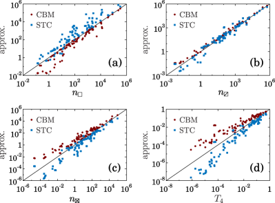
Refer to caption
Figure 8: The CBM and STC [Eqs. (26-29)] approximations to the (a) density of 444-loops, (b) density of diamonds, (c) density of 444-cliques, and (d) 444-transitivity, as a function of the actual observed values in a varied dataset of 95 real-world networks. In each panel one marker corresponds to one network.

To further assess the validity of the approximate relations derived from the STC model, a comparison with other models of clustered networks is worthwhile. As mentioned in Sec. I, most existing mathematically tractable models of clustered networks involve a random linking of triangles, complete or partial cliques, or other higher-order motifs. Unfortunately most of these models are not easily fitted to real networks, therefore the range of applicability of relations derived within them is not easily established. One clique-based model where this can actually be done in a particularly elegant manner is due to Gleeson [21]. In this model each node belongs to exactly one clique and any number of external links. Importantly, the joint degree and clique size distribution in this model can be exactly fitted to a given network degree distribution and clustering spectrum CKsubscript𝐶𝐾C_{K}. For this reason we chose this model, as a representative of clique-based models, to compare our results to, and we will refer to it as clique-based model (CBM). In the CBM the quantities nsubscript𝑛n_{\leavevmode\hbox to4.4pt{\vbox to4.4pt{\pgfpicture\makeatletter\hbox{\hskip 0.2pt\lower-0.2pt\hbox to0.0pt{\pgfsys@beginscope\pgfsys@invoke{ }\definecolor{pgfstrokecolor}{rgb}{0,0,0}\pgfsys@color@rgb@stroke{0}{0}{0}\pgfsys@invoke{ }\pgfsys@color@rgb@fill{0}{0}{0}\pgfsys@invoke{ }\pgfsys@setlinewidth{0.4pt}\pgfsys@invoke{ }\nullfont\hbox to0.0pt{\pgfsys@beginscope\pgfsys@invoke{ }{{}{{}}{} {}{{}}{}{}{}{}{{}}{}{}\pgfsys@moveto{0.0pt}{0.0pt}\pgfsys@moveto{0.0pt}{0.0pt}\pgfsys@lineto{0.0pt}{4.0pt}\pgfsys@lineto{4.0pt}{4.0pt}\pgfsys@lineto{4.0pt}{0.0pt}\pgfsys@closepath\pgfsys@moveto{4.0pt}{4.0pt}\pgfsys@stroke\pgfsys@invoke{ } } \pgfsys@invoke{\lxSVG@closescope }\pgfsys@endscope{}{}{}\hss}\pgfsys@discardpath\pgfsys@invoke{\lxSVG@closescope }\pgfsys@endscope\hss}}\lxSVG@closescope\endpgfpicture}}}, nsubscript𝑛n_{\leavevmode\hbox to4.4pt{\vbox to4.4pt{\pgfpicture\makeatletter\hbox{\hskip 0.2pt\lower-0.2pt\hbox to0.0pt{\pgfsys@beginscope\pgfsys@invoke{ }\definecolor{pgfstrokecolor}{rgb}{0,0,0}\pgfsys@color@rgb@stroke{0}{0}{0}\pgfsys@invoke{ }\pgfsys@color@rgb@fill{0}{0}{0}\pgfsys@invoke{ }\pgfsys@setlinewidth{0.4pt}\pgfsys@invoke{ }\nullfont\hbox to0.0pt{\pgfsys@beginscope\pgfsys@invoke{ }{{}{{}}{} {}{{}}{}{}{}{}{{}}{}{}\pgfsys@moveto{0.0pt}{0.0pt}\pgfsys@moveto{0.0pt}{0.0pt}\pgfsys@lineto{0.0pt}{4.0pt}\pgfsys@lineto{4.0pt}{4.0pt}\pgfsys@lineto{4.0pt}{0.0pt}\pgfsys@closepath\pgfsys@moveto{4.0pt}{4.0pt}\pgfsys@stroke\pgfsys@invoke{ } {}{{}}{} {}{}{}\pgfsys@moveto{0.0pt}{0.0pt}\pgfsys@lineto{4.0pt}{4.0pt}\pgfsys@stroke\pgfsys@invoke{ } } \pgfsys@invoke{\lxSVG@closescope }\pgfsys@endscope{}{}{}\hss}\pgfsys@discardpath\pgfsys@invoke{\lxSVG@closescope }\pgfsys@endscope\hss}}\lxSVG@closescope\endpgfpicture}}}, nsubscript𝑛n_{\leavevmode\hbox to4.4pt{\vbox to4.4pt{\pgfpicture\makeatletter\hbox{\hskip 0.2pt\lower-0.2pt\hbox to0.0pt{\pgfsys@beginscope\pgfsys@invoke{ }\definecolor{pgfstrokecolor}{rgb}{0,0,0}\pgfsys@color@rgb@stroke{0}{0}{0}\pgfsys@invoke{ }\pgfsys@color@rgb@fill{0}{0}{0}\pgfsys@invoke{ }\pgfsys@setlinewidth{0.4pt}\pgfsys@invoke{ }\nullfont\hbox to0.0pt{\pgfsys@beginscope\pgfsys@invoke{ }{{}{{}}{} {}{{}}{}{}{}{}{{}}{}{}\pgfsys@moveto{0.0pt}{0.0pt}\pgfsys@moveto{0.0pt}{0.0pt}\pgfsys@lineto{0.0pt}{4.0pt}\pgfsys@lineto{4.0pt}{4.0pt}\pgfsys@lineto{4.0pt}{0.0pt}\pgfsys@closepath\pgfsys@moveto{4.0pt}{4.0pt}\pgfsys@stroke\pgfsys@invoke{ } {}{{}}{} {}{}{}\pgfsys@moveto{0.0pt}{0.0pt}\pgfsys@lineto{4.0pt}{4.0pt}\pgfsys@stroke\pgfsys@invoke{ } {{}{}}{{}}{} {{}{}}{}{}\pgfsys@moveto{0.0pt}{4.0pt}\pgfsys@lineto{4.0pt}{0.0pt}\pgfsys@stroke\pgfsys@invoke{ } } \pgfsys@invoke{\lxSVG@closescope }\pgfsys@endscope{}{}{}\hss}\pgfsys@discardpath\pgfsys@invoke{\lxSVG@closescope }\pgfsys@endscope\hss}}\lxSVG@closescope\endpgfpicture}}} and T4subscript𝑇4T_{4} are easily calculated as functions of the moments of the clique-size distribution, which we fitted to the clustering spectra of the 95 real networks considered. The resulting values are presented in FIG. 8. While both the CBM and STC models produce reasonable approximations 666It is important to remark that the relations derived from the STC model are universal and did not require any parameter fitting, while the values for the CBM were obtained by fitting the entire degree distribution and clustering spectrum of a real network., there are interesting differences to be considered.

The differences are due to the fact that the CBM and STC models realize, in a sense, two opposite extreme approaches to producing clustered networks. In the CBM, triangles only exist within complete cliques, and this leads to an overestimation of denser motifs, e.g., 444-cliques and an underestimation of sparser motifs such as 444-loops. On the other hand, in the STC model triangles are produced in a more homogeneous, diffuse manner, resulting in the opposite trend: an underestimation of 444-cliques and an overestimation of 444-loops777Another comparison of real world clustering statistics with Gleeson’s model and a different kind of random model, using rewiring and also matching the clustering spectrum, was made in Ref. [43]..

A quantity that sharply highlights the difference between the two models is the normalized ratio Rsubscript𝑅R_{\operatorname{\mkern 1.0mu\leavevmode\hbox to4.4pt{\vbox to4.4pt{\pgfpicture\makeatletter\hbox{\hskip 0.2pt\lower-0.2pt\hbox to0.0pt{\pgfsys@beginscope\pgfsys@invoke{ }\definecolor{pgfstrokecolor}{rgb}{0,0,0}\pgfsys@color@rgb@stroke{0}{0}{0}\pgfsys@invoke{ }\pgfsys@color@rgb@fill{0}{0}{0}\pgfsys@invoke{ }\pgfsys@setlinewidth{0.4pt}\pgfsys@invoke{ }\nullfont\hbox to0.0pt{\pgfsys@beginscope\pgfsys@invoke{ }{{}{{}}{} {}{{}}{}{}{}{}{{}}{}{}\pgfsys@moveto{0.0pt}{0.0pt}\pgfsys@moveto{0.0pt}{0.0pt}\pgfsys@lineto{0.0pt}{4.0pt}\pgfsys@lineto{4.0pt}{4.0pt}\pgfsys@lineto{4.0pt}{0.0pt}\pgfsys@closepath\pgfsys@moveto{4.0pt}{4.0pt}\pgfsys@stroke\pgfsys@invoke{ } {}{{}}{} {}{}{}\pgfsys@moveto{0.0pt}{0.0pt}\pgfsys@lineto{4.0pt}{4.0pt}\pgfsys@stroke\pgfsys@invoke{ } } \pgfsys@invoke{\lxSVG@closescope }\pgfsys@endscope{}{}{}\hss}\pgfsys@discardpath\pgfsys@invoke{\lxSVG@closescope }\pgfsys@endscope\hss}}\lxSVG@closescope\endpgfpicture}}}} of the number of diamonds to 444-loops [see Eq. (17)]. This quantity always has the trivial value R(CBM)=1superscriptsubscript𝑅(CBM)1R_{\operatorname{\mkern 1.0mu\leavevmode\hbox to4.4pt{\vbox to4.4pt{\pgfpicture\makeatletter\hbox{\hskip 0.2pt\lower-0.2pt\hbox to0.0pt{\pgfsys@beginscope\pgfsys@invoke{ }\definecolor{pgfstrokecolor}{rgb}{0,0,0}\pgfsys@color@rgb@stroke{0}{0}{0}\pgfsys@invoke{ }\pgfsys@color@rgb@fill{0}{0}{0}\pgfsys@invoke{ }\pgfsys@setlinewidth{0.4pt}\pgfsys@invoke{ }\nullfont\hbox to0.0pt{\pgfsys@beginscope\pgfsys@invoke{ }{{}{{}}{} {}{{}}{}{}{}{}{{}}{}{}\pgfsys@moveto{0.0pt}{0.0pt}\pgfsys@moveto{0.0pt}{0.0pt}\pgfsys@lineto{0.0pt}{4.0pt}\pgfsys@lineto{4.0pt}{4.0pt}\pgfsys@lineto{4.0pt}{0.0pt}\pgfsys@closepath\pgfsys@moveto{4.0pt}{4.0pt}\pgfsys@stroke\pgfsys@invoke{ } {}{{}}{} {}{}{}\pgfsys@moveto{0.0pt}{0.0pt}\pgfsys@lineto{4.0pt}{4.0pt}\pgfsys@stroke\pgfsys@invoke{ } } \pgfsys@invoke{\lxSVG@closescope }\pgfsys@endscope{}{}{}\hss}\pgfsys@discardpath\pgfsys@invoke{\lxSVG@closescope }\pgfsys@endscope\hss}}\lxSVG@closescope\endpgfpicture}}}}^{\textrm{(CBM)}}=1 in clique-based network models (made of complete cliques), since one 444-loop corresponds to exactly two diamond motifs in this case. This property of clique-based models, demonstrating the extreme concentration of triangles, is clearly at odds with structures observed in real-world network data. In the STC model, using the assumptions outlined at the beginning of this section, this ratio is simply given by the transitivity, R(STC)Tsuperscriptsubscript𝑅(STC)𝑇R_{\operatorname{\mkern 1.0mu\leavevmode\hbox to4.4pt{\vbox to4.4pt{\pgfpicture\makeatletter\hbox{\hskip 0.2pt\lower-0.2pt\hbox to0.0pt{\pgfsys@beginscope\pgfsys@invoke{ }\definecolor{pgfstrokecolor}{rgb}{0,0,0}\pgfsys@color@rgb@stroke{0}{0}{0}\pgfsys@invoke{ }\pgfsys@color@rgb@fill{0}{0}{0}\pgfsys@invoke{ }\pgfsys@setlinewidth{0.4pt}\pgfsys@invoke{ }\nullfont\hbox to0.0pt{\pgfsys@beginscope\pgfsys@invoke{ }{{}{{}}{} {}{{}}{}{}{}{}{{}}{}{}\pgfsys@moveto{0.0pt}{0.0pt}\pgfsys@moveto{0.0pt}{0.0pt}\pgfsys@lineto{0.0pt}{4.0pt}\pgfsys@lineto{4.0pt}{4.0pt}\pgfsys@lineto{4.0pt}{0.0pt}\pgfsys@closepath\pgfsys@moveto{4.0pt}{4.0pt}\pgfsys@stroke\pgfsys@invoke{ } {}{{}}{} {}{}{}\pgfsys@moveto{0.0pt}{0.0pt}\pgfsys@lineto{4.0pt}{4.0pt}\pgfsys@stroke\pgfsys@invoke{ } } \pgfsys@invoke{\lxSVG@closescope }\pgfsys@endscope{}{}{}\hss}\pgfsys@discardpath\pgfsys@invoke{\lxSVG@closescope }\pgfsys@endscope\hss}}\lxSVG@closescope\endpgfpicture}}}}^{\textrm{(STC)}}\approx T. FIG. 9 shows that, for the 95 real-world networks considered, the STC model provides reasonable approximations for Rsubscript𝑅R_{\operatorname{\mkern 1.0mu\leavevmode\hbox to4.4pt{\vbox to4.4pt{\pgfpicture\makeatletter\hbox{\hskip 0.2pt\lower-0.2pt\hbox to0.0pt{\pgfsys@beginscope\pgfsys@invoke{ }\definecolor{pgfstrokecolor}{rgb}{0,0,0}\pgfsys@color@rgb@stroke{0}{0}{0}\pgfsys@invoke{ }\pgfsys@color@rgb@fill{0}{0}{0}\pgfsys@invoke{ }\pgfsys@setlinewidth{0.4pt}\pgfsys@invoke{ }\nullfont\hbox to0.0pt{\pgfsys@beginscope\pgfsys@invoke{ }{{}{{}}{} {}{{}}{}{}{}{}{{}}{}{}\pgfsys@moveto{0.0pt}{0.0pt}\pgfsys@moveto{0.0pt}{0.0pt}\pgfsys@lineto{0.0pt}{4.0pt}\pgfsys@lineto{4.0pt}{4.0pt}\pgfsys@lineto{4.0pt}{0.0pt}\pgfsys@closepath\pgfsys@moveto{4.0pt}{4.0pt}\pgfsys@stroke\pgfsys@invoke{ } {}{{}}{} {}{}{}\pgfsys@moveto{0.0pt}{0.0pt}\pgfsys@lineto{4.0pt}{4.0pt}\pgfsys@stroke\pgfsys@invoke{ } } \pgfsys@invoke{\lxSVG@closescope }\pgfsys@endscope{}{}{}\hss}\pgfsys@discardpath\pgfsys@invoke{\lxSVG@closescope }\pgfsys@endscope\hss}}\lxSVG@closescope\endpgfpicture}}}} in some cases, although in general underestimates the true values.
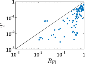
Refer to caption
Figure 9: The STC approximation (Tabsent𝑇\approx T) to the ratio Rsubscript𝑅R_{\operatorname{\mkern 1.0mu\leavevmode\hbox to4.4pt{\vbox to4.4pt{\pgfpicture\makeatletter\hbox{\hskip 0.2pt\lower-0.2pt\hbox to0.0pt{\pgfsys@beginscope\pgfsys@invoke{ }\definecolor{pgfstrokecolor}{rgb}{0,0,0}\pgfsys@color@rgb@stroke{0}{0}{0}\pgfsys@invoke{ }\pgfsys@color@rgb@fill{0}{0}{0}\pgfsys@invoke{ }\pgfsys@setlinewidth{0.4pt}\pgfsys@invoke{ }\nullfont\hbox to0.0pt{\pgfsys@beginscope\pgfsys@invoke{ }{{}{{}}{} {}{{}}{}{}{}{}{{}}{}{}\pgfsys@moveto{0.0pt}{0.0pt}\pgfsys@moveto{0.0pt}{0.0pt}\pgfsys@lineto{0.0pt}{4.0pt}\pgfsys@lineto{4.0pt}{4.0pt}\pgfsys@lineto{4.0pt}{0.0pt}\pgfsys@closepath\pgfsys@moveto{4.0pt}{4.0pt}\pgfsys@stroke\pgfsys@invoke{ } {}{{}}{} {}{}{}\pgfsys@moveto{0.0pt}{0.0pt}\pgfsys@lineto{4.0pt}{4.0pt}\pgfsys@stroke\pgfsys@invoke{ } } \pgfsys@invoke{\lxSVG@closescope }\pgfsys@endscope{}{}{}\hss}\pgfsys@discardpath\pgfsys@invoke{\lxSVG@closescope }\pgfsys@endscope\hss}}\lxSVG@closescope\endpgfpicture}}}} [see Eq. (17)], as a function of the actual observed value in a varied dataset of 95 real-world networks. One marker corresponds to one network.

These results suggest that more realistic versions of the STC model may be achieved by adopting a non-homogeneous triadic closure mechanism, where the probability of closing a triad depends on local structural properties. An obvious candidate for such local properties to consider would be node degrees: in general one may prescribe an arbitrary function f(k1,k2,k3)𝑓subscript𝑘1subscript𝑘2subscript𝑘3f(k_{1},k_{2},k_{3}) for the probability of closing a triad of degrees k1,k2,k3subscript𝑘1subscript𝑘2subscript𝑘3k_{1},k_{2},k_{3}. This would allow for substantial control over the extent to which triangles overlap to form loopy motifs, and would allow for the modelling of various forms of the clustering spectrum CKsubscript𝐶𝐾C_{K}.

VII Discussion and conclusions

In this paper we studied in detail a static model of random clustered networks based on the mechanism of triadic closure. In particular, we start from a “backbone” network of arbitrary degree distribution and, with a given probability f𝑓f, we close each of the existing triads. In the case where the backbone is an uncorrelated locally treelike network, due to its simplicity this model allows for exact analytical results regarding clustering properties of the network.

We found an exact expression for transitivity and we showed anomalous behavior of this quantity in large power-law degree-distributed networks; transitivity is equal to 00 in the infinite size limit for degree distribution exponent γ<5/2𝛾52\gamma<5/2 and transitivity is equal to f𝑓f for 5/2<γ452𝛾45/2<\gamma\leq 4.

This sharp transition is reminiscent of another transition occurring for this value of γ𝛾\gamma. Indeed, the largest eigenvalue of the adjacency matrix (spectral radius) of power-law networks is k2/kkc3γsimilar-todelimited-⟨⟩superscript𝑘2delimited-⟨⟩𝑘superscriptsubscript𝑘𝑐3𝛾\langle k^{2}\rangle/\langle k\rangle\sim k_{c}^{3-\gamma} for γ<5/2𝛾52\gamma<5/2, while it is kc1/2superscriptsubscript𝑘𝑐12k_{c}^{1/2} for γ>5/2𝛾52\gamma>5/2 [44, 45]. In that case, the transition is related to the localization of the principal eigenvector of the adjacency matrix, either on the K-core of maximum index or on the largest hub and its nearest neighbors [46]. The identification of the role of interbranch and intrabranch triads in the behavior of transitivity provides a complementary and clarifying view. In networks with γ<5/2𝛾52\gamma<5/2 a large max K-core is present. In such structures the neighbors of nodes with large degree have many neighbors in their turn. This is reflected by the dominance of interbranch processes in the STC model. For γ>5/2𝛾52\gamma>5/2 instead, the spectral radius is determined by the largest hub and its direct neighbors, which tend to have a small number of neighbors. Correspondingly the transitivity is dominated by the formation of connections among the hub’s neighbors (intrabranch processes).

To quantify the density of higher order cliques we defined a generalized transitivity Tnsubscript𝑇𝑛T_{n} as the number of n𝑛n-cliques in the network relative to their maximum possible number (in perfect analogy to standard transitivity). We found an exact expression for the general Tnsubscript𝑇𝑛T_{n} and showed that this quantity undergoes a discontinuous transition—analogous to the standard case—at γ(n)=31/(n1)subscriptsuperscript𝛾𝑛31𝑛1\gamma^{*}_{(n)}=3-1/(n-1).

Using generating functions and simple combinatorial considerations we found exact expressions for the densities of various small loopy motifs, as functions of the first few moments of the backbone degree distribution. Importantly, all motifs in the STC model are produced by triangles (closed triads) overlapping in various ways, i.e., all emerging small-scale structures are purely induced by the random triadic closure mechanism. This circumstance makes the STC model a useful tool to evaluate the plausibility of the triadic closure mechanism in real-world networks. With some reasonable assumptions about the moments of the degree distribution, we derived some universal relations between the densities of small loopy motifs. Specifically, we were able to express the density of various motifs involving four nodes as a function of transitivity and of the third moment of the degree distribution. We showed that these remarkably simple, universal relations, hold up reasonably well in real-world networks.

Many interesting research avenues, opened by this work, deserve further investigation. First, while this paper focuses on global quantities, it would be important to understand in detail also the behavior of local quantities, such as the degree distribution PKsubscript𝑃𝐾P_{K}, the local clustering coefficient Cisubscript𝐶𝑖C_{i}, and degree-degree correlations. Second, the generalization of the approach used in [36] for percolation on the STC model with f=1𝑓1f=1 can provide insight into the behavior of percolation and other processes on networks with strong clustering and many short loops. Finally, the STC procedure can be generalized to build hypergraphs, by considering not only the edges created by the STC mechanism but also the triangles, as well as higher-order motifs, as hyperedges. The motif counting analysis developed in this work can be straightforwardly generalized in this case, providing a nontrivial, yet exactly solvable, model for triadic interaction.

Appendix A Probability generating functions

A.1 General definitions

Given a discrete probability distribution fksubscript𝑓𝑘f_{k}, the associated generating function is defined as

g(z)=zk=kfkzk,𝑔𝑧delimited-⟨⟩superscript𝑧𝑘subscript𝑘subscript𝑓𝑘superscript𝑧𝑘g(z)=\langle z^{k}\rangle=\sum_{k}f_{k}z^{k}, (30)

where the sum is intended over the whole range of k𝑘k values for which fksubscript𝑓𝑘f_{k} is defined. In case of a continuous variable with probability density f(k)𝑓𝑘f(k), we define

g(z)=𝑑kf(k)zk.𝑔𝑧differential-d𝑘𝑓𝑘superscript𝑧𝑘g(z)=\int dkf(k)z^{k}. (31)

For our purposes, we consider the degree distribution pk=Nk/Nsubscript𝑝𝑘subscript𝑁𝑘𝑁p_{k}=N_{k}/N, where Nksubscript𝑁𝑘N_{k} is the number of nodes with degree k𝑘k, with k[kmin,kc(N)]𝑘subscript𝑘minsubscript𝑘𝑐𝑁k\in[k_{\text{min}},k_{c}(N)], where kc(N)subscript𝑘𝑐𝑁k_{c}(N) diverges in the infinite-size limit. We denote by g0(z)subscript𝑔0𝑧g_{0}(z) the degree distribution generating function. Another useful distribution to consider is qrsubscript𝑞𝑟q_{r}, where the random variable r𝑟r is the so-called excess degree, i.e., the degree of a node at which we arrive following a randomly chosen edge excluding the edge we arrived from. We can express qrsubscript𝑞𝑟q_{r} in terms of pksubscript𝑝𝑘p_{k}. Indeed, we can compute the probability of reaching a node of excess degree r𝑟r, and hence degree r+1𝑟1r+1, following a randomly chosen edge. This is simply given by

qr=(r+1)Nr+1r(r+1)Nr+1=(r+1)pr+1k.subscript𝑞𝑟𝑟1subscript𝑁𝑟1subscript𝑟𝑟1subscript𝑁𝑟1𝑟1subscript𝑝𝑟1delimited-⟨⟩𝑘q_{r}=\frac{(r+1)N_{r+1}}{\sum_{r}(r+1)N_{r+1}}=\frac{(r+1)p_{r+1}}{\langle k\rangle}. (32)

This expression allows us to express the generating function g1(z)=rqrzrsubscript𝑔1𝑧subscript𝑟subscript𝑞𝑟superscript𝑧𝑟g_{1}(z)=\sum_{r}q_{r}z^{r} in terms of g0subscript𝑔0g_{0} by

g1(z)=g0(z)g0(1).subscript𝑔1𝑧superscriptsubscript𝑔0𝑧superscriptsubscript𝑔01g_{1}(z)=\frac{g_{0}^{\prime}(z)}{g_{0}^{\prime}(1)}. (33)

A.2 Analytic and asymptotic methods

Given a generating function g0(z)subscript𝑔0𝑧g_{0}(z) it is possible to obtain the coefficients pksubscript𝑝𝑘p_{k}, i.e. the probability distribution pksubscript𝑝𝑘p_{k}, by differentiation [6]

pk=1k!dkdzkg0(z)|z=0=12πi𝒞dzg0(z)zk+1,p_{k}=\frac{1}{k!}\frac{d^{k}}{dz^{k}}g_{0}(z)\big{\rvert}_{z=0}=\frac{1}{2\pi i}\oint_{\mathcal{C}}dz\frac{g_{0}(z)}{z^{k+1}}, (34)

where 𝒞𝒞\mathcal{C} is an arbitrary path around the origin in the complex z𝑧z plane. It is quite rare that this procedure can be carried out explicitly for any k𝑘k. Nevertheless, complex analysis developed many tools to estimate the asymptotics of the coefficients pksubscript𝑝𝑘p_{k} for large k𝑘k. For instance, if g0(z)subscript𝑔0𝑧g_{0}(z) is analytic, then g1(z)subscript𝑔1𝑧g_{1}(z) is also analytic and the composition of analytic functions is analytic too. Hence we know for sure that PKsubscript𝑃𝐾P_{K} cannot exhibit a power-law tail [47]. If instead the generating function g0(z)subscript𝑔0𝑧g_{0}(z) exhibits a singular behavior for z1𝑧superscript1z\to 1^{-}, it is possible to know the asymptotic behavior of the coefficients of the series expansion around z=0𝑧0z=0, that is the asymptotics of pksubscript𝑝𝑘p_{k} for large k𝑘k. In particular, we recall the following result (Theorem 1 and its corollaries in [48]): if f(z)=nfnzn𝑓𝑧subscript𝑛subscript𝑓𝑛superscript𝑧𝑛f(z)=\sum_{n}f_{n}z^{n} is analytical in the unitary circle in the complex plane excluding z0=1subscript𝑧01z_{0}=1, and as z1𝑧1z\to 1 in this domain, f(z)c(1z)αsimilar-to𝑓𝑧𝑐superscript1𝑧𝛼f(z)\sim c(1-z)^{\alpha} for α𝛼\alpha real, then for noninteger α𝛼\alpha we have

fncΓ(α)nα1,n.formulae-sequencesimilar-tosubscript𝑓𝑛𝑐Γ𝛼superscript𝑛𝛼1𝑛f_{n}\sim\frac{c}{\Gamma(-\alpha)}n^{-\alpha-1},~{}~{}~{}n\to\infty. (35)

Hence for a singular g0(z)subscript𝑔0𝑧g_{0}(z) it is sufficient to expand around 1, using ϵ=1zitalic-ϵ1𝑧\epsilon=1-z as a small parameter, to get the asymptotic form of pksubscript𝑝𝑘p_{k}.

A.2.1 The degree distribution of Gfsubscript𝐺𝑓G_{f} with PL backbone

Using Eq. (35) and the expansions for the generating functions of a PL degree distribution

g0(1ε)subscript𝑔01𝜀\displaystyle g_{0}(1-\varepsilon) 1kε+12kBε2+C(γ1)εγ1,similar-to-or-equalsabsent1delimited-⟨⟩𝑘𝜀12delimited-⟨⟩𝑘𝐵superscript𝜀2𝐶𝛾1superscript𝜀𝛾1\displaystyle\simeq 1-\langle k\rangle\varepsilon+\frac{1}{2}\langle k\rangle B\varepsilon^{2}+C(\gamma-1)\varepsilon^{\gamma-1},
g1(1ε)subscript𝑔11𝜀\displaystyle g_{1}(1-\varepsilon) 1Bε+12Dε2+C(γ2)εγ2,similar-to-or-equalsabsent1𝐵𝜀12𝐷superscript𝜀2𝐶𝛾2superscript𝜀𝛾2\displaystyle\simeq 1-B\varepsilon+\frac{1}{2}D\varepsilon^{2}+C(\gamma-2)\varepsilon^{\gamma-2},

where B𝐵B, D𝐷D and C𝐶C are constants depending on γ𝛾\gamma and kminsubscript𝑘mink_{\text{min}}888See Appendix G in [36] for their explicit values and, in particular, their signs depending on the value of γ𝛾\gamma., from Eq. (1) we get

G0(1ϵ)1[k+fkB]ϵ+kC(γ2)(fϵ)γ2.similar-to-or-equalssubscript𝐺01italic-ϵ1delimited-[]delimited-⟨⟩𝑘𝑓delimited-⟨⟩𝑘𝐵italic-ϵdelimited-⟨⟩𝑘𝐶𝛾2superscript𝑓italic-ϵ𝛾2\displaystyle G_{0}(1-\epsilon)\simeq 1-[\langle k\rangle+f\langle k\rangle B]\epsilon+\langle k\rangle C(\gamma-2)(f\epsilon)^{\gamma-2}. (36)

From Eq. (35) we get for K𝐾K\to\infty

PKsubscript𝑃𝐾\displaystyle P_{K} kC(γ2)fγ2Γ(2γ)K(γ1),similar-toabsentdelimited-⟨⟩𝑘𝐶𝛾2superscript𝑓𝛾2Γ2𝛾superscript𝐾𝛾1\displaystyle\sim\frac{\langle k\rangle C(\gamma-2)f^{\gamma-2}}{\Gamma(2-\gamma)}K^{-(\gamma-1)},

from which we conclude that the STC procedure on PL backbones with exponent γ𝛾\gamma produces (asymptotically) PL networks with exponent γ=γ1superscript𝛾𝛾1\gamma^{\prime}=\gamma-1.

A.3 Computing averages using generating functions

Generating functions are useful tools because they contain information about the whole probability distribution in a very compact way [47]999From [47],“A generating function is a clothesline on which we hang up a sequence of numbers [probabilities] for display.”. Indeed, taking the derivatives of the generating functions we can evaluate averages. It is easy to see that, defining the n𝑛n-th factorial moment [49] μn=k(k1)(kn+1)subscript𝜇𝑛delimited-⟨⟩𝑘𝑘1𝑘𝑛1\mu_{n}=\langle k(k-1)\dots(k-n+1)\rangle

μnsubscript𝜇𝑛\displaystyle\mu_{n} =[(ddz)ng0(z)]|z=1,absentevaluated-atdelimited-[]superscript𝑑𝑑𝑧𝑛subscript𝑔0𝑧𝑧1\displaystyle=\left[\left(\frac{d}{dz}\right)^{n}g_{0}(z)\right]\biggr{|}_{z=1}, (37)
kndelimited-⟨⟩superscript𝑘𝑛\displaystyle\langle k^{n}\rangle =[(zddz)ng0(z)]|z=1,absentevaluated-atdelimited-[]superscript𝑧𝑑𝑑𝑧𝑛subscript𝑔0𝑧𝑧1\displaystyle=\left[\left(z\frac{d}{dz}\right)^{n}g_{0}(z)\right]\biggr{|}_{z=1}, (38)

where we used the fact that g0(z)=zk=eklnzsubscript𝑔0𝑧delimited-⟨⟩superscript𝑧𝑘delimited-⟨⟩superscript𝑒𝑘𝑧g_{0}(z)=\langle z^{k}\rangle=\langle e^{k\ln z}\rangle and zd/dz=d/d(lnz)𝑧𝑑𝑑𝑧𝑑𝑑𝑧zd/dz=d/d(\ln z).

It is possible to express kndelimited-⟨⟩superscript𝑘𝑛\langle k^{n}\rangle as a linear combination of μjsubscript𝜇𝑗\mu_{j} for jn𝑗𝑛j\leq n using the relation [50]

(zddz)nf(z)=j=1n{nj}zj(ddz)jf(z),superscript𝑧𝑑𝑑𝑧𝑛𝑓𝑧superscriptsubscript𝑗1𝑛FRACOP𝑛𝑗superscript𝑧𝑗superscript𝑑𝑑𝑧𝑗𝑓𝑧\left(z\frac{d}{dz}\right)^{n}\!\!f(z)=\sum_{j=1}^{n}\genfrac{\{}{\}}{0.0pt}{}{n}{j}z^{j}\left(\frac{d}{dz}\right)^{j}\!\!f(z), (39)

where {nj}FRACOP𝑛𝑗\genfrac{\{}{\}}{0.0pt}{}{n}{j} denote the Stirling numbers of the second kind, whose expression is given by [47, 50]

{nj}=i=1j(1)jiini!(ji)!.FRACOP𝑛𝑗superscriptsubscript𝑖1𝑗superscript1𝑗𝑖superscript𝑖𝑛𝑖𝑗𝑖\genfrac{\{}{\}}{0.0pt}{}{n}{j}=\sum_{i=1}^{j}\frac{(-1)^{j-i}i^{n}}{i!(j-i)!}.

Evaluating Eq. (39) for f(z)=g0(z)𝑓𝑧subscript𝑔0𝑧f(z)=g_{0}(z) at z=1𝑧1z=1 we get

kn=j=1n{nj}μj.delimited-⟨⟩superscript𝑘𝑛superscriptsubscript𝑗1𝑛FRACOP𝑛𝑗subscript𝜇𝑗\langle k^{n}\rangle=\sum_{j=1}^{n}\genfrac{\{}{\}}{0.0pt}{}{n}{j}\mu_{j}. (40)

Remarkably, Eq. (40) states for ER networks, for which μj=cjsubscript𝜇𝑗superscript𝑐𝑗\mu_{j}=c^{j}, that

kn=j=1n{nj}cj,delimited-⟨⟩superscript𝑘𝑛superscriptsubscript𝑗1𝑛FRACOP𝑛𝑗superscript𝑐𝑗\langle k^{n}\rangle=\sum_{j=1}^{n}\genfrac{\{}{\}}{0.0pt}{}{n}{j}c^{j},

that is kndelimited-⟨⟩superscript𝑘𝑛\langle k^{n}\rangle is a power series in c𝑐c whose coefficients are the Stirling numbers of the second kind.

On the other hand, it is possible to express μnsubscript𝜇𝑛\mu_{n} in terms of kndelimited-⟨⟩superscript𝑘𝑛\langle k^{n}\rangle for jn𝑗𝑛j\leq n using the Stirling numbers of the first kind [nj]FRACOP𝑛𝑗\genfrac{[}{]}{0.0pt}{}{n}{j} which are defined by the relation [51]

j=0n1(xj)=j=1n(1)nj[nj]xj.superscriptsubscriptproduct𝑗0𝑛1𝑥𝑗superscriptsubscript𝑗1𝑛superscript1𝑛𝑗FRACOP𝑛𝑗superscript𝑥𝑗\prod_{j=0}^{n-1}(x-j)=\sum_{j=1}^{n}(-1)^{n-j}\genfrac{[}{]}{0.0pt}{}{n}{j}x^{j}. (41)

Evaluating Eq. (41) for x=k𝑥𝑘x=k and averaging over pksubscript𝑝𝑘p_{k} we get

μn=j=1n(1)nj[nj]kj.subscript𝜇𝑛superscriptsubscript𝑗1𝑛superscript1𝑛𝑗FRACOP𝑛𝑗delimited-⟨⟩superscript𝑘𝑗\mu_{n}=\sum_{j=1}^{n}(-1)^{n-j}\genfrac{[}{]}{0.0pt}{}{n}{j}\langle k^{j}\rangle. (42)

Appendix B Moments of power-law distributions

Given a power law probability distribution pkkγsimilar-tosubscript𝑝𝑘superscript𝑘𝛾p_{k}\sim k^{-\gamma} with k[kmin,kc]𝑘subscript𝑘minsubscript𝑘𝑐k\in[k_{\text{min}},k_{c}], we have

pk=kγζ(γ,kmin)ζ(γ,kc)kγζ(γ,kmin),subscript𝑝𝑘superscript𝑘𝛾𝜁𝛾subscript𝑘min𝜁𝛾subscript𝑘𝑐similar-to-or-equalssuperscript𝑘𝛾𝜁𝛾subscript𝑘minp_{k}=\frac{k^{-\gamma}}{\zeta(\gamma,k_{\text{min}})-\zeta(\gamma,k_{c})}\simeq\frac{k^{-\gamma}}{\zeta(\gamma,k_{\text{min}})}, (43)

where ζ(γ,x)=kxkγ𝜁𝛾𝑥subscript𝑘𝑥superscript𝑘𝛾\zeta(\gamma,x)=\sum_{k\geq x}k^{-\gamma} is the Hurwitz zeta function [52]. The moments of the distribution are given by

kn=ζ(γn,kmin)ζ(γn,kc)ζ(γ,kmin)ζ(γ,kc).delimited-⟨⟩superscript𝑘𝑛𝜁𝛾𝑛subscript𝑘min𝜁𝛾𝑛subscript𝑘𝑐𝜁𝛾subscript𝑘min𝜁𝛾subscript𝑘𝑐\langle k^{n}\rangle=\frac{\zeta(\gamma-n,k_{\text{min}})-\zeta(\gamma-n,k_{c})}{\zeta(\gamma,k_{\text{min}})-\zeta(\gamma,k_{c})}. (44)

To make computations less cumbersome, we can adopt the continuous-degree approximation, in which the degree is assumed to be a continuous variable. Note that the larger the value of kminsubscript𝑘mink_{\text{min}}, the better this approximation works. We have

pksubscript𝑝𝑘\displaystyle p_{k} =(γ1)kminγ1[1(kminkc)γ1]kγ(γ1)kminγ1kγ,absent𝛾1superscriptsubscript𝑘min𝛾1delimited-[]1superscriptsubscript𝑘minsubscript𝑘𝑐𝛾1superscript𝑘𝛾similar-to-or-equals𝛾1superscriptsubscript𝑘min𝛾1superscript𝑘𝛾\displaystyle=\frac{(\gamma-1)k_{\text{min}}^{\gamma-1}}{\left[1-\left(\frac{k_{\text{min}}}{k_{c}}\right)^{\gamma-1}\right]}k^{-\gamma}\simeq(\gamma-1)k_{\text{min}}^{\gamma-1}k^{-\gamma}, (45)
kdelimited-⟨⟩𝑘\displaystyle\langle k\rangle =γ1γ2kmin[1(kminkc)γ2]γ1γ2kmin,absent𝛾1𝛾2subscript𝑘mindelimited-[]1superscriptsubscript𝑘minsubscript𝑘𝑐𝛾2similar-to-or-equals𝛾1𝛾2subscript𝑘min\displaystyle=\frac{\gamma-1}{\gamma-2}k_{\text{min}}\left[1-\left(\frac{k_{\text{min}}}{k_{c}}\right)^{\gamma-2}\right]\simeq\frac{\gamma-1}{\gamma-2}k_{\text{min}}, (46)

for γ>2𝛾2\gamma>2 and kckminmuch-greater-thansubscript𝑘𝑐subscript𝑘mink_{c}\gg k_{\text{min}}, which is the case we consider in this paper. For higher order moments of the distribution, the result depends on the value of γ𝛾\gamma, since the n𝑛n-th moment may diverge. We have, for kckminmuch-greater-thansubscript𝑘𝑐subscript𝑘mink_{c}\gg k_{\text{min}}

kndelimited-⟨⟩superscript𝑘𝑛\displaystyle\langle k^{n}\rangle =(γ1)kminγ1γn+1[kminn(γ1)kcn(γ1)]absent𝛾1superscriptsubscript𝑘min𝛾1𝛾𝑛1delimited-[]superscriptsubscript𝑘min𝑛𝛾1superscriptsubscript𝑘𝑐𝑛𝛾1\displaystyle=\frac{(\gamma-1)k_{\text{min}}^{\gamma-1}}{\gamma-n+1}\left[k_{\text{min}}^{n-(\gamma-1)}-k_{c}^{n-(\gamma-1)}\right] (47)
kckmin{γ1γ1nkminn if n<γ1,γ1n+1γkminγ1kcn(γ1) if n>γ1.much-greater-thansubscript𝑘𝑐subscript𝑘minsimilar-to-or-equalscases𝛾1𝛾1𝑛superscriptsubscript𝑘min𝑛 if 𝑛𝛾1𝛾1𝑛1𝛾superscriptsubscript𝑘min𝛾1superscriptsubscript𝑘𝑐𝑛𝛾1 if 𝑛𝛾1\displaystyle\underset{k_{c}\gg k_{\text{min}}}{\simeq}\begin{cases}\frac{\gamma-1}{\gamma-1-n}k_{\text{min}}^{n}&\text{ if }n<\gamma-1,\\ \frac{\gamma-1}{n+1-\gamma}k_{\text{min}}^{\gamma-1}k_{c}^{n-(\gamma-1)}&\text{ if }n>\gamma-1.\end{cases} (48)

Note that μnknsimilar-tosubscript𝜇𝑛delimited-⟨⟩superscript𝑘𝑛\mu_{n}\sim\langle k^{n}\rangle is finite for n<γ1𝑛𝛾1n<\gamma-1: in such a case, it is useful to have an explicit expression for μnsubscript𝜇𝑛\mu_{n}, at least for n=1,2,3,4𝑛1234n=1,2,3,4, those encountered in the main text. Using Eq. (42) and [51] we get

μ1subscript𝜇1\displaystyle\mu_{1} =k,absentdelimited-⟨⟩𝑘\displaystyle=\langle k\rangle, (49)
μ2subscript𝜇2\displaystyle\mu_{2} =k2k,absentdelimited-⟨⟩superscript𝑘2delimited-⟨⟩𝑘\displaystyle=\langle k^{2}\rangle-\langle k\rangle, (50)
μ3subscript𝜇3\displaystyle\mu_{3} =k33k2+2k,absentdelimited-⟨⟩superscript𝑘33delimited-⟨⟩superscript𝑘22delimited-⟨⟩𝑘\displaystyle=\langle k^{3}\rangle-3\langle k^{2}\rangle+2\langle k\rangle, (51)
μ4subscript𝜇4\displaystyle\mu_{4} =k46k3+11k26k.absentdelimited-⟨⟩superscript𝑘46delimited-⟨⟩superscript𝑘311delimited-⟨⟩superscript𝑘26delimited-⟨⟩𝑘\displaystyle=\langle k^{4}\rangle-6\langle k^{3}\rangle+11\langle k^{2}\rangle-6\langle k\rangle. (52)

For n>γ1𝑛𝛾1n>\gamma-1 instead we have

μnγ1n+1γkminγ1kcn(γ1).similar-to-or-equalssubscript𝜇𝑛𝛾1𝑛1𝛾superscriptsubscript𝑘min𝛾1superscriptsubscript𝑘𝑐𝑛𝛾1\displaystyle\mu_{n}\simeq\frac{\gamma-1}{n+1-\gamma}k_{\text{min}}^{\gamma-1}k_{c}^{n-(\gamma-1)}. (53)

Appendix C High-order moments of PKsubscript𝑃𝐾P_{K}

From Eq. (1) and Eqs. (37)-(38), we can compute, at least in principle, every average with respect to PKsubscript𝑃𝐾P_{K} in 𝒢fsubscript𝒢𝑓\mathcal{G}_{f}, in terms of averages with respect to pksubscript𝑝𝑘p_{k}. It is possible to obtain an explicit expression for Mn=K(K1)(Kn+1)=G0(n)(1)subscript𝑀𝑛delimited-⟨⟩𝐾𝐾1𝐾𝑛1superscriptsubscript𝐺0𝑛1M_{n}=\langle K(K-1)\dots(K-n+1)\rangle=G_{0}^{(n)}(1) for arbitrary n𝑛n using the Faà di Bruno’s formula for the n𝑛n-th derivative of a composite function [53]. Denoting with Dn=(d/dz)nsuperscript𝐷𝑛superscript𝑑𝑑𝑧𝑛D^{n}=(d/dz)^{n}, we have

Dn[f(u(z))]=n!m=1nf(m)(u(z))m!i1++im=nj=1mu(ij)(z)ij!.superscript𝐷𝑛delimited-[]𝑓𝑢𝑧𝑛superscriptsubscript𝑚1𝑛superscript𝑓𝑚𝑢𝑧𝑚subscriptsubscript𝑖1subscript𝑖𝑚𝑛superscriptsubscriptproduct𝑗1𝑚superscript𝑢subscript𝑖𝑗𝑧subscript𝑖𝑗D^{n}\left[f(u(z))\right]=n!\sum_{m=1}^{n}\frac{f^{(m)}(u(z))}{m!}\!\!\!\sum_{i_{1}+\dots+i_{m}=n}\prod_{j=1}^{m}\frac{u^{(i_{j})}(z)}{i_{j}!}. (54)

Writing G0(z)=g0(ψ(z))subscript𝐺0𝑧subscript𝑔0𝜓𝑧G_{0}(z)=g_{0}(\psi(z)), where ψ(z)=zg1(1f+fz)𝜓𝑧𝑧subscript𝑔11𝑓𝑓𝑧\psi(z)=zg_{1}(1-f+fz), it is easy to prove by induction that

ψ(n)(z)=nfn1g1(n1)(1f+fz)+fnzg1(n)(1f+fz).superscript𝜓𝑛𝑧𝑛superscript𝑓𝑛1superscriptsubscript𝑔1𝑛11𝑓𝑓𝑧superscript𝑓𝑛𝑧subscriptsuperscript𝑔𝑛11𝑓𝑓𝑧\psi^{(n)}(z)=nf^{n-1}g_{1}^{(n-1)}\big{(}1-f+fz\big{)}+f^{n}zg^{(n)}_{1}\big{(}1-f+fz\big{)}. (55)

From Eq. (54) with f=g0𝑓subscript𝑔0f=g_{0} and u=ψ𝑢𝜓u=\psi evaluated at z=1𝑧1z=1 we finally get, using Eqs. (33)(37),(55)

Mn=n!m=1nμmm!s1++sm=nj=1m[sjfsj1μsj+fsjμsj+1]μ1sj!.subscript𝑀𝑛𝑛superscriptsubscript𝑚1𝑛subscript𝜇𝑚𝑚subscriptsubscript𝑠1subscript𝑠𝑚𝑛superscriptsubscriptproduct𝑗1𝑚delimited-[]subscript𝑠𝑗superscript𝑓subscript𝑠𝑗1subscript𝜇subscript𝑠𝑗superscript𝑓subscript𝑠𝑗subscript𝜇subscript𝑠𝑗1subscript𝜇1subscript𝑠𝑗M_{n}=n!\!\sum_{m=1}^{n}\frac{\mu_{m}}{m!}\!\!\sum_{s_{1}+\dots+s_{m}=n}\prod_{j=1}^{m}\frac{[s_{j}f^{s_{j}-1}\mu_{s_{j}}+f^{s_{j}}\mu_{s_{j}+1}]}{\mu_{1}s_{j}!}. (56)

Eq. (56) allows us to compute the expected number of n1𝑛1n-1-stars and the generalized transitivity Tnsubscript𝑇𝑛T_{n} for arbitrary n>1𝑛1n>1 (see Sec. V.2), but the computation becomes soon cumbersome. Nevertheless, with Eq. (56) we can prove Eq.(23). In the case of PL backbones with 2<γ<32𝛾32<\gamma<3, we have μjkcj+1γsimilar-tosubscript𝜇𝑗superscriptsubscript𝑘𝑐𝑗1𝛾\mu_{j}\sim k_{c}^{j+1-\gamma} for j>1𝑗1j>1, while μ11similar-tosubscript𝜇11\mu_{1}\sim 1, and ψ(j)(1)fjkcj+2γsimilar-tosuperscript𝜓𝑗1superscript𝑓𝑗superscriptsubscript𝑘𝑐𝑗2𝛾\psi^{(j)}(1)\sim f^{j}k_{c}^{j+2-\gamma} for j1𝑗1j\geq 1. From Eq. (56) we obtain

Mnafnkcn+2γ+m=2nbmfmkcm+1γ+m(3γ),similar-to-or-equalssubscript𝑀𝑛𝑎superscript𝑓𝑛superscriptsubscript𝑘𝑐𝑛2𝛾superscriptsubscript𝑚2𝑛subscript𝑏𝑚superscript𝑓𝑚superscriptsubscript𝑘𝑐𝑚1𝛾𝑚3𝛾M_{n}\simeq af^{n}k_{c}^{n+2-\gamma}+\sum_{m=2}^{n}b_{m}f^{m}k_{c}^{m+1-\gamma+m(3-\gamma)}, (57)

where a,bm𝑎subscript𝑏𝑚a,b_{m} are constants. The exponent α=m+1γ+m(3γ)𝛼𝑚1𝛾𝑚3𝛾\alpha=m+1-\gamma+m(3-\gamma) is a monotonically increasing function in m𝑚m, hence its maximum value is reached for mα=nsubscript𝑚𝛼𝑛m_{\alpha}=n. Thus we have

Mnafnkcn+2γ+bnfnkcn+1γ+n(3γ).similar-to-or-equalssubscript𝑀𝑛𝑎superscript𝑓𝑛superscriptsubscript𝑘𝑐𝑛2𝛾subscript𝑏𝑛superscript𝑓𝑛superscriptsubscript𝑘𝑐𝑛1𝛾𝑛3𝛾M_{n}\simeq af^{n}k_{c}^{n+2-\gamma}+b_{n}f^{n}k_{c}^{n+1-\gamma+n(3-\gamma)}. (58)

The second term on the r.h.s. dominates for 2<γ<31/n2𝛾31𝑛2<\gamma<3-1/n, while the first term dominates for γ>31/n𝛾31𝑛\gamma>3-1/n. For γ>n+2𝛾𝑛2\gamma>n+2, none of the terms appearing in Eq. (56) diverges, hence G0(n)(1)1similar-tosuperscriptsubscript𝐺0𝑛11G_{0}^{(n)}(1)\sim 1. Finally, for 31/n<γ<n+231𝑛𝛾𝑛23-1/n<\gamma<n+2 the leading term is always given by kcn+2γsuperscriptsubscript𝑘𝑐𝑛2𝛾k_{c}^{n+2-\gamma}: some of the terms in the sum on the r.h.s. of are Eq. (57) ψsj1similar-tosuperscript𝜓subscript𝑠𝑗1\psi^{s_{j}}\sim 1, hence the exponent will be lower than α𝛼\alpha, and since α<n+2γ𝛼𝑛2𝛾\alpha<n+2-\gamma we can conclude that the leading order is given by the first term. With the substitution nn1𝑛𝑛1n\to n-1 this yields Eq. (23).

Notice that for 3<γ<43𝛾43<\gamma<4, since MnKnsimilar-tosubscript𝑀𝑛delimited-⟨⟩superscript𝐾𝑛M_{n}\sim\langle K^{n}\rangle and kn+1kcn+1γsimilar-todelimited-⟨⟩superscript𝑘𝑛1superscriptsubscript𝑘𝑐𝑛1𝛾\langle k^{n+1}\rangle\sim k_{c}^{n+1-\gamma}, Eq. (58) implies that, for kckminmuch-greater-thansubscript𝑘𝑐subscript𝑘mink_{c}\gg k_{\text{min}}, Knfnknsimilar-todelimited-⟨⟩superscript𝐾𝑛superscript𝑓𝑛delimited-⟨⟩superscript𝑘𝑛\langle K^{n}\rangle\sim f^{n}\langle k^{n}\rangle, as stated in Sec. VI.

References