See pages 1 of Cover.pdf

To my grandparents

Chapter 1 Introduction

In the early 1980s, heavy-ion collisions were proposed as a means to provide a window into the inner workings of the early universe. In particular, it was hoped that these kinds of experiments would be able to produce a deconfined state of matter with quarks and gluons as the fundamental degrees of freedom. Around that time, Bjorken posited that objects known as jets, high-energy sprays of collimated hadrons would interact with such a state of matter if it were produced in these collisions and in doing so, would become extinguished or quenched [3]. Indeed, it has been over 20 years since the phenomenon of jet quenching was first observed at RHIC, providing strong evidence that for the existence of a quark-gluon plasma (QGP) in heavy-ion collisions [4, 5].

In recent years, the arrival of more powerful experiments at the LHC and RHIC has put us in a position where we can reasonably ask sharp questions concerning the make-up and the nature of the QGP, thereby definitively moving on from solely pondering its existence. Nevertheless, it goes without saying that with such progress comes the need to improve the accuracy of our theoretical models to the stage where they can make pointed, meaningful predictions.

As an example, consider the phenomenon of transverse momentum broadening: in traversing the QGP, a jet receives kicks in transverse momentum space, giving rise to a diffusive process, characterised by the transverse momentum broadening coefficient, $\hat{q}$. It recently has been suggested that such momentum broadening effects may be imprinted on the jet acoplanarity observable [6, 7, 8, 9, 10]. Moreover, $\hat{q}$ has an indirect but strong influence on the production of medium-induced radiation. Quantum corrections to $\hat{q}$ (at $\mathcal{O}(g^{2})$) have drawn a significant amount of attention over the past ten years or so since it was realised that they have the potential to be logarithmically enhanced [1, 2]. We follow this line of enquiry here, computing these logarithmic corrections using thermal field theory. In doing so, we rigorously analyse how the thermal scale affects the region of phase space from which these corrections are borne. Another important advancement in improving the quantification of jet quenching phenomena has come with the development of a resummation method, which provides a non-perturbative evaluation of the classical contributions to transverse momentum broadening [11, 12, 13, 14].

The asymptotic mass, $m_{\infty}$ is a correction to a hard parton’s dispersion relation as it forward scatters with plasma constituents and is also known to control in part the mechanism of medium-induced radiation. The computation of non-perturbative corrections to $m_{\infty}$ is firmly underway [15, 16]. In computing quantum corrections to $m_{\infty}$ (also at $\mathcal{O}(g^{2})$) in the thermal field theory framework, we concretely further this program. We complete a matching calculation, which eliminates unphysical infinities from the previously computed non-perturbative evaluation while also beginning the full computation of the $\mathcal{O}(g^{2})$ corrections.

This thesis is organised in such a way to slowly but surely build up the intuition and introduce the tools that are needed to understand the reasonably technical computations of quantum corrections to the aforementioned quantities that come in the later chapters. Specifically, the thesis is laid out as follows:

• Starting from the basics of quantum field theory, Ch. 2 is intended to convince the reader of the existence of a QGP in heavy-ion collisions through the provision of both theoretical arguments and experimental evidence. Along the way, we introduce the concept of jets and describe the different stages of a heavy-ion collision.

• In Ch. 3, we set up the physical picture, which is helpful to keep in mind throughout the rest of the thesis. Namely, a jet, which for our purposes can be taken as a hard parton, propagates through a quark-gluon plasma, interacting with the medium constituents and in doing so, is forced to radiate. We make a point to emphasise how the triggering mechanism for this radiation is controlled by the associated formation time and we identify the conditions under which Landau-Pomeranchuk-Migdal (LPM) interference must be accounted for. We furthermore compute the radiation rate in the multiple scattering regime, where LPM resummation is necessary and in the single scattering regime, where one can instead use the opacity expansion. The chapter closes with a brief overview of the literature and a short discussion of some recent developments.

• Ch 4 introduces some of the modern theoretical tools, which support the calculations to follow in the later chapters. In particular, we give some general ideas regarding the basics of effective field theories and thermal field theory before moving on to discuss the finite-temperature effective theories EQCD and HTL theory. In Sec. 4.3, we examine how a seminal idea from Caron-Huot [17] can, in certain situations, provide an extremely useful connection between these two theories, which furthermore allows for the non-perturbative computation of classical corrections to the transverse momentum broadening kernel and the asymptotic mass. The chapter then continues with a demonstration of how this idea can also be utilised to efficiently extract the leading order soft contributions to the transverse momentum broadening kernel and the asymptotic mass.

• Ch 5 is largely based on the work [18]. There, we carefully scrutinise the previous computations of double logarithmic corrections to $\hat{q}$ [1, 2] before showing how the double logarithmic phase space is deformed for a computation done in the setting of a weakly coupled quark-gluon plasma. In addition, we clearly demonstrate how this region of phase space is situated with respect to the one from which the classical corrections to $\hat{q}$ emerge. Most of our computation is performed in the harmonic oscillator approximation. However, a pathway, which could allow us to go beyond this approximation is also presented. Technical details are contained in App. C.

• Ch 6 contains our yet to be published work on the $\mathcal{O}(g^{2})$ asymptotic mass corrections. We list all the diagrams that can contribute at this order of perturbation theory, before arguing that only one of them, what we label as diagram $(c)$ contributes. We show how some of the IR divergences associated with this diagram cancel with corresponding UV divergences from the EQCD calculation, completed in [16]. We then proceed to a computation of the full fermionic and gluonic parts of diagram $(c)$, which turn out to contain some unforeseen UV and collinear divergences. Technical details are contained in App. D.

• A broad summary and conclusion are given in Ch. 7 in addition to discussions of how we plan to push the works contained in Chs. 5 and  6 further.

• Our conventions are specified in App. A and some details on the basics of Wilson loops are located in App. B.

Chapter 2 QCD and Heavy-Ion Collisions

The Standard Model of Particle Physics is arguably one of the greatest intellectual achievements to have come out of the $20\textsuperscript{th}$ century. While it is not expected to be the end of the story as far as elementary physics is concerned, the well-tested Standard Model provides a remarkably clean and coherent description of three out of the four fundamental forces: the electromagnetic and weak forces, which are unified into the Electroweak Theory as well as the strong force, described by Quantum Chromodynamics (QCD). This thesis is concerned with the study of the latter.

In this first chapter, we introduce QCD in Sec. 2.1 through a somewhat formal lens before discussing some of its properties. In Secs. 2.2 and 2.3 we highlight how some of these properties manifest themselves in systems with a large number of particles. Sec. 2.4 is then devoted to a discussion of heavy-ion collisions, which have proved extremely successful in aiding the experimental exploration of the QCD phase diagram. This is intended to appropriately set up and motivate what is to follow in the rest of the thesis, where we study in great detail how jets, high energy showers of radiation interact with the quark-gluon plasma.

2.1 Introduction to QCD

Locality is generally considered to be an essential feature of any (fundamental) quantum field theory (QFT). However, by insisting on a theory to be local, a certain redundancy is necessarily introduced. This redundancy manifests itself in the Lagrangian description as what is known as gauge freedom. To understand this in a more concrete way, consider what happens when we demand that a Lagrangian describing $N_{f}$ fermionic fields, $\psi_{i}(X)$ ($i=1,2,...,N_{f}$) remain invariant under the local transformation

$$\psi_{i}(X)\rightarrow\psi^{\prime}_{i}(X)=\mathcal{U}(X)\psi_{i}(X),\quad\quad\mathcal{U}=\exp(i\xi^{a}(X)T_{F}^{a}),\quad\quad a=1,2,..,d_{A},$$ (2.1)

with a sum over $a$ implied. The transformation, $\mathcal{U}$ is said to be in the fundamental representation of the Lie group SU($N_{c}$), meaning in practice that $\mathcal{U}(X)$ is an $N_{c}\times N_{c}$ unitary matrix with $\det\mathcal{U}=1$. Since SU($N_{c}$) is a topologically trivial group, the matrices $\mathcal{U}$ are given in terms of the so-called generators, $T_{F}^{a}$, which are in the fundamental representation of the $\mathfrak{su}(N_{c})$ Lie algebra. The $\xi_{a}(X)$ are then arbitrary functions of spacetime coordinates. The fact that the $T_{R}^{a}$ generate a Lie algebra means that they obey, for a general representation, $R$

$$[T_{R}^{a},T_{R}^{b}] =if^{abc}T_{R}^{c}.$$ (2.2)

$$f^{abd}f^{dce} +f^{bcd}f^{dae}+f^{cad}f^{dbe}=0$$ (2.3)

If the structure constants $f^{abc}$ are zero, then the matrices, $\mathcal{U}(X)$ are in a representation of an Abelian group. Otherwise, the group is said to be non-Abelian, which is the case that we are presently interested in. Moreover, we have that

$$T_{R}^{a}T_{R}^{a}=C_{R}\mathbb{I},\quad\quad\Tr T_{R}^{a}T_{R}^{b}=T_{R}\delta^{ab},$$ (2.4)

where $C_{R},T_{R}$ are respectively the Casimir and index of the representation, $R$.

At this point, it is easy to see that a mass term for the quark fields, i.e $m\bar{\psi}_{i}\psi_{i}$ is invariant under the transformation Eq. (2.1). Be that as it may, because of the spacetime dependence in $\mathcal{U}(X)$, any term with a derivative acting on $\psi_{i}$ will not be so fortunate since

$$\partial_{\mu}\psi_{i}(X)\rightarrow\Big{[}\partial_{\mu}\psi_{i}(X)\Big{]}^{\prime}=\mathcal{U}(X)\partial_{\mu}\psi_{i}(X)+\Big{(}\partial_{\mu}\mathcal{U}(X)\Big{)}\psi_{i}(X).$$ (2.5)

To fix the kinetic term, we must define a covariant derivative operator, $D_{\mu}$ such that

$$D_{\mu}\psi_{i}(X)\rightarrow\Big{[}\partial_{\mu}\psi_{i}(X)\Big{]}^{\prime}=\mathcal{U}(X)D_{\mu}\psi_{i}(X).$$ (2.6)

It turns out that the covariant derivative should take the form

$$D_{\mu}=\partial_{i}-igA_{\mu},$$ (2.7)

where $A_{\mu}=A_{\mu}^{a}T_{F}^{a}$ is a Lie-algebra-valued gauge field and $g$ is the (bare) coupling constant that characterises the strength of the interaction between this field and $\psi$. It transforms in such a way

$$A_{\mu}(X)\rightarrow A^{\prime}_{\mu}(X)=\mathcal{U}(X)A_{\mu}(X)\mathcal{U}^{-1}(X)-\frac{i}{g}\Big{(}\partial_{\mu}\mathcal{U}(X)\Big{)}\mathcal{U}^{-1}(X)$$ (2.8)

to ensure that Eq. (2.6) holds true. The gauge field is said to transform according to the adjoint representation of SU($N_{c}$), modified by an inhomogeneous term (the second term above). The adjoint representation of a group is defined such that the generators are given in terms of the structure constants themselves

$$(T^{a}_{A})^{bc}=-if^{abc},$$ (2.9)

where these are now $d_{A}\times d_{A}$ matrices.

Quantity	Symbol	Value for QCD
Number of matter fields	$N_{f}$	$6$
Number of charges	$N_{c}$	3
Fundamental Casimir	$C_{F}=\frac{N^{2}_{c}-1}{2N_{c}}$	$\frac{4}{3}$
Adjoint Casimir	$C_{A}=N_{c}$	$3$
Fundamental index	$T_{F}=\frac{1}{2}$	$\frac{1}{2}$
Adjoint index	$T_{A}=N_{c}$	$3$
Fundamental dimension	$d_{F}=N_{c}$	$3$
Adjoint dimension	$d_{A}=N_{c}^{2}-1$	$8$

Table 2.1: Collection of group theory factors, specific to QCD, intended to be used for future reference. Note that while $6$ flavours of quarks are included in the Standard Model, oftentimes perturbative calculations are performed with $N_{f}<6$ if the energy scale of interest is much smaller than the heavier quarks.

To briefly recap, by insisting on a Lagrangian description of a field $\psi$ that is blind to local, non-Abelian phases, the Lagrangian is forced to be furthermore invariant under the transformation Eq. (2.8) – it is forced to be gauge-invariant. Under these restrictions, the resultant theory that one derives, describing the interaction between dynamical gauge and matter fields goes by the name of Yang-Mills Theory [19].

It turns out that Yang-Mills theory with $N_{c}=3$ colours and $N_{f}=6$ flavours yields a theory that describes well the strong interaction, which is responsible for the binding of nucleons inside atomic nuclei. The colours: red, green and blue are non-Abelian charges and are mediated by the gluon field, $A_{\mu}$. Each flavour corresponds to a different quark field: up, down, strange, charm, bottom, top, listed from least to most massive. The resultant theory is known as Quantum Chromodynamics and is given by the Lagrangian [20] constructed to be suitably gauge-invariant and renormalisable

$$\mathcal{L}_{\text{QCD}}=-\frac{1}{4}F^{a}_{\mu\nu}F^{\mu\nu\,a}+\bar{\psi}_{i}(i\not{D}-m_{i})\psi_{i},$$ (2.10)

with a sum over $i$ implied. The field strength tensor is

$$F_{\mu\nu}^{a}=\partial_{\mu}A_{\nu}-\partial_{\nu}A_{\mu}+gf^{abc}A^{b}_{\mu}A^{c}_{\nu}$$ (2.11)

and $g$ is the strong coupling constant. An immediately remarkable aspect of Eq. (2.10) is that of the self-interactions between gluons, a feature, which is not present in QCD’s Abelian counterpart, Quantum Electrodynamics (QED).

Eq. (2.10) should be considered the Lagrangian for classical QCD. The quantisation of non-Abelian gauge theories is usually done using the functional integral formalism. Along the way, one runs into the issue of gauge-fixing at the level of the path integral, which is dealt with by introducing so-called ghost fields in the Fadeev-Popov procedure. We refer the reader to any of the textbooks [21, 22, 23] for the details pertaining to the quantisation procedure.

In the form of Eq. (2.10), QCD does not possess any predictive power beyond tree-level – it must be renormalised. Divergences that emerge at one-loop level and beyond can be absorbed by replacing the bare coupling constants of the theory, $g_{i}$ renormalised couplings, $g_{i}(\mu)$, which now depend on an additional scale, $\mu$. The idea is then to demand that physical observables be independent of this scale, which gives rise to a set of coupled differential equations known as renormalisation group equations (RGE). The RGE for the strong coupling reads

$$\frac{dg(\mu)}{d\mu}=\beta(g(\mu)),$$ (2.12)

where the $\beta$-function, defined above, can be calculated order by order in perturbation theory. At one-loop level, one finds [24, 25]

$$\beta(g(\mu))_{\text{one-loop}}=-\frac{g^{3}(\mu)}{16\pi^{2}}\beta_{0},\quad\quad\beta_{0}\equiv\bigg{(}\frac{11}{3}C_{A}-\frac{4}{3}N_{f}T_{F}\bigg{)},$$ (2.13)

from which one can proceed to solve Eq. (2.12). The solution can be written as

$$\alpha_{s}(\mu)=\frac{4\pi}{\beta_{0}}\frac{1}{\ln\frac{\mu^{2}}{\Lambda^{2}_{\text{QCD}}}},\quad\quad\alpha_{s}\equiv\frac{g^{2}}{4\pi},$$ (2.14)

and is understood to only be valid for $\mu>\Lambda_{\text{QCD}}$. Two very striking features of QCD are brought to light by this equation:

• As $\mu$ increases, the coupling gets weaker, signifying that QCD is asymptotically free.

• As $\mu$ approaches the scale $\Lambda_{\text{QCD}}$, the coupling diverges, giving rise to what is known as a Landau Pole. This suggests that perturbative QCD should not be trusted at these energies and moreover, it hints at the confining nature of QCD, why free quarks and gluons and hence, coloured particles are never observed in nature.

The QCD $\beta$-function is currently known up to five-loop [26, 27, 28, 29]. With this value in hand and the 2018 “world-average” value $\alpha_{s}(M_{Z}^{2})=0.1181\pm 0.0011$ [30], given in the $\overline{\text{MS}}$ subtraction scheme, one finds $\Lambda^{(6)}_{\text{QCD}}=(89\pm 6)\text{MeV}$, where the apex denotes that such a calculation takes $N_{f}=6$.

If one takes the colour confinement hypothesis seriously, then it follows that only colour singlets – states that are invariant under rotations in colour space should be observed in nature. Such states are known as hadrons. Hadrons are divided up into two categories: baryons, which are bound states of three quarks and mesons, which are bound states of a quark and an anti-quark.

Before moving on, let us go back to Eq. (2.10) and consider its global symmetries, i.e, transformations under which it is invariant that are not spacetime dependent. Moreover, let us neglect for the moment the quark masses, which is not such a bad approximation if we consider energies much larger than $\Lambda_{\text{QCD}}$. Then we can rewrite it as

$$\mathcal{L}_{\text{QCD}}=-\frac{1}{4}F^{a}_{\mu\nu}F^{\mu\nu\,a}+i\Big{[}\bar{\psi}_{i\,R}\not{D}\psi_{i\,R}+\bar{\psi}_{i\,L}\not{D}\psi_{i\,L}\Big{]},$$ (2.15)

where the chiral spinors are defined using the projectors $\psi_{i\,R/L}=\frac{1}{2}(1\pm\gamma_{5})\psi_{i}$. As well as Poincaré invariance, the quark sector is invariant under transformations belonging to the group

$$\mathcal{G}=\text{U}(1)_{V}\times\text{U}(1)_{A}\times\text{SU}(N_{f})_{L}\times\text{SU}(N_{f})_{R}.$$

$\mathcal{G}$ acts on the quark fields such that

$$\text{U}(1)_{V} :\quad\quad\psi_{L}\to e^{i\alpha}\psi_{L}\quad,\quad\psi_{R}\to e^{i\alpha}\psi_{R}$$

$$\text{U}(1)_{A} :\quad\quad\psi_{L}\to e^{i\beta}\psi_{L}\quad,\quad\psi_{R}\to e^{-i\beta}\psi_{R}$$

$$\text{SU}(N_{f})_{L} :\quad\quad\psi_{L}\to L\psi_{L}\quad,\quad\psi_{R}\to\psi_{R}$$

$$\text{SU}(N_{f})_{R} :\quad\quad\psi_{L}\to\psi_{L}\quad,\quad\psi_{R}\to R\psi_{R}$$

where $L,R$ are $N_{f}\times N_{f}$ matrices. Through Noether’s Theorem, the abelian vector symmetry is associated with baryon number conservation. In contrast, when quantising the theory, one finds that the path integral measure is not invariant under the axial abelian symmetry, resulting in what is known as a chiral anomaly [31, 32]. As for the non-abelian symmetries, consider the vacuum expectation value $\Delta=\langle\bar{\psi}_{i\,L}\psi_{j\,R}\rangle$, also known as the chiral condensate, which has been shown to be non-zero by Lattice QCD calculations [33]. It is not hard to see that this quantity is only invariant under transformations such that $L^{\dagger}=R$, implying that the chiral symmetry is spontaneously broken into the diagonal subgroup:

$$\text{SU}(N_{f})_{L}\times\text{SU}(N_{f})_{R}\to\text{SU}(N_{f})_{V},$$

where the pions are the Nambu-Goldstone bosons tied to the symmetry breaking.

We have up to this point discussed two kinds of transitions associated with the theory of QCD: confinement and chiral symmetry breaking, either side of which the fundamental degrees of freedom of the theory are clearly very different. Indeed, this points to the fact that QCD has a rich phase structure. We will come back to this point in Sec. 2.3, after we discuss what has been a historically successful testbed for perturbative QCD.

2.2 Jets

Confinement greatly obstructs the prospect of ever being able to directly observe free quarks and gluons, which we collectively refer to as partons. Even though free partons are briefly produced in collider experiments, once their virtualities decrease to the scale of $\Lambda_{\text{QCD}}$, they are expected to hadronise. So how can we ever expect to test perturbative QCD (pQCD) experimentally? Fortunately, the idea of quark-hadron duality, originally formulated by Poggio, Quinn and Weinberg [35] suggests that certain inclusive hadronic cross-sections at high energies, being appropriately averaged over an energy range should coincide with what one calculates in pQCD. Because of this, one can use objects known as jets to test the perturbative sector of QCD, without having a precise, fundamental description of the hadronisation process.

In, for instance, $e^{+}e^{-}$ collisions or proton-proton (p-p) collisions, one can have rare, hard processes take place where large amounts of momentum are exchanged between participating constituents. The output of such a process, which is calculable in perturbative QCD, is a high-energy parton with large virtuality, $Q$. The way in which the parton radiates to shed its virtuality can in principle be calculated order by order in $\alpha_{s}$. However, it is more practical and furthermore accurate to seek a result, which instead focuses on including the contribution from certain regions of phase space, which greatly enhance higher order terms in the $\alpha_{s}$ expansion. The regions of phase space that we are talking about here are associated with collinear and soft emissions. By following such an approach, which is well-explained in the textbook [37], the following picture emerges: the highly-virtual parton splits repeatedly, giving rise to what is known as a parton shower. The splitting, which generates the parton shower can be modelled as a Markovian process and can be readily implemented in Monte-Carlo event generator.

The shower does not produce an incoherent splatter of particles but rather, because of the soft, collinear enhancements, a cone-like object. It is this self-collimated structure, which defines a jet. This is often referred to as angular-ordered showering and is in fact a general feature of gauge theories. Therefore, this phenomenon also takes place in QED showers. However, the showering is accentuated for the case of QCD, due to the self-interacting gluon field, which is a novel feature of Eq. (2.10). Indeed, three jet events in $e^{+}e^{-}$ collisions provided the first direct evidence of the existence of the gluon and the quark-gluon vertex [38, 39].

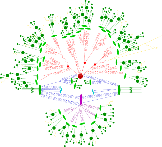
Figure 2.1: Illustration of a hadron-hadron collision, taken from [40]. The incoming green blobs represent the initial hadronic states. Blue lines denote initial-state radiation, which is not discussed in the main text. The red and purple blobs are the sites at which the hard interactions take place and the lines emanating from them represent the parton shower. Hadronisation processes are marked by the light-green blobs whereas dark-green blobs mark hadron decays. Yellow lines signal soft photon radiation. Note that the angles associated with the parton splittings are greatly exaggerated above.

There are a number of Monte-Carlo event generators on the market built to simulate parton showers in addition to the underlying hadron-hadron collision. Nevertheless, since hadrons are the objects that are measured in detectors, how can one be sure that the description provided by parton showers is accurate? To bridge the connection between theoretical, pQCD predictions and experimental observations, one needs to invoke a jet definition. Jet definitions provide an algorithm through which experimentalists are able to cluster final-state particles together. The act of clustering leads to the reconstruction of the jet, all the way back to the initial hard interaction point. The method through which the final state particles are clustered should moreover be defined in such a way that is robust to the addition of an arbitrary number of soft particles – it should be IR safe. Sequential recombination algorithms cluster particles in an iterative manner, according to some protocol until no particle remains. Examples include the Cambridge/Aachen [45], $k_{t}$ [46] and anti-$k_{t}$ [47] algorithms. Alternatively, there exist cone algorithms [48], where one searches for stable cones where the jet axis and jet momentum align. See [49] for a review.

Nowadays, the study of jets in $e^{+}e^{-}$ and $p-p$ collisions is considered to be a mature field, leaning on the side of what can be regarded as precision physics. Indeed, the ATLAS and CMS experiments at the LHC even try to search for physics beyond the Standard Model (BSM) by taking advantage of this level of precision [50, 51, 52, 53, 54]. While we are not concerned with such a line of enquiry here, it is important to emphasise that the behaviour of jets in $p-p$ collisions or rather, jets in vacuum can be used as a reference point when comparing to how jets behave in heavy-ion collisions, a topic, which we will move on to discuss shortly.

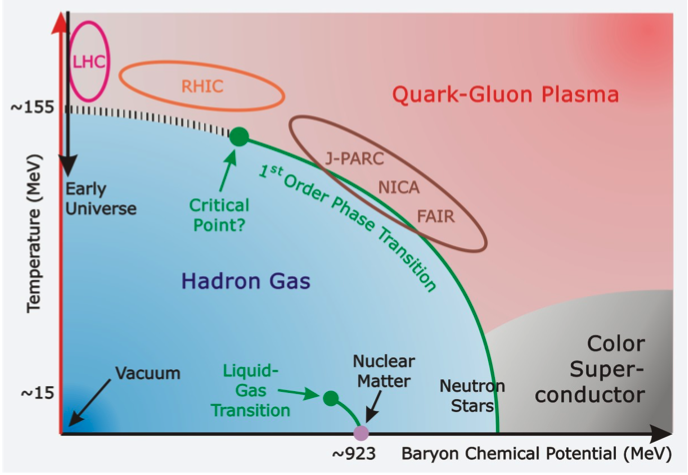
Figure 2.2: Sketch of the QCD phase diagram, taken from [55]. Close to the $\mu_{B}=0$ axis, the transition from confined to deconfined matter, known as the quark-gluon plasma, is expected to be a smooth crossover. A hypothesised critical point then separates this region from the one where a first-order transition is expected. Moving further to the right, there is the possibility of a colour superconducting phase. The transition from the nuclear matter we observe at room temperature, well-described by the Liquid-Drop Model [56, 57] to the so-called Hadron Resonance Gas, composed of free nucleons is located at around $T=15\text{MeV}$ [58].

2.3 QCD Phase Diagram

During Sec. 2.1, we discussed some of the basic features of QCD. Here, we progress to explore the QCD phase diagram, first considered in [59, 60]. A sketch is given in Fig. 2.2. The $y$-axis is temperature, $T$ whereas the $x$-axis denotes baryon chemical potential, $\mu_{B}$, conjugate to the baryon number

$$\text{B}=\frac{1}{3}(N_{q}-N_{\bar{q}})$$ (2.16)

and can be thought of as a proxy for density. Our aim here is not to provide a comprehensive review of the phase diagram but to explain some of its general features. We follow the reviews [61, 62, 63] closely.

In general, to obtain a quantitative understanding of a phase transition, one needs to identify an order parameter. In Sec. 2.1, the chiral condensate was mentioned, which can be thought of as an order parameter characterising the chiral phase transition. For the confinement-deconfinement transition, in the approximation where quarks are not dynamical (or rather infinitely heavy), a parameter often used is the Polyakov Loop [64], derived in the setting of Euclidean spacetime. It is given as (see App. B for a short introduction to Wilson lines)

$$L(\vec{\mathbf{x}})=\mathcal{P}\exp\Big(ig\int_{0}^{\beta}d\tau A_{4}(\tau,\vec{\mathbf{x}})\Big{missing}),\quad\quad l(\vec{\mathbf{x}})=\frac{1}{N_{c}}\Tr L(\vec{\mathbf{x}}),\quad\quad\Phi\equiv\langle l\rangle$$ (2.17)

where $\tau=it$ and $A_{4}$ is the Euclidean temporal component of the gauge field. It has been argued [65, 66] that this temporal Wilson line can be related to the heavy quark potential, $f_{\bar{q}q}$

$$\langle l^{\dagger}(\vec{\mathbf{x}}^{\prime})l(\vec{\mathbf{x}})\rangle=C\exp\Big(-\frac{1}{T}f_{\bar{q}q}(|\vec{\mathbf{x}}^{\prime}-\vec{\mathbf{x}}|)\Big{missing})$$ (2.18)

through what is known as the Polyakov loop correlation function. In the confining phase, the potential should have a linearly rising potential, i.e $f_{\bar{q}q}(r)=\sigma r$ so that the correlation function decays exponentially at large separation. On the other hand, in the deconfined phase, the inter-quark potential is thermally screened so that $f_{\bar{q}q}(r\to\infty)=\text{const.}$, which yields a non-zero value for the correlation function. We can then state schematically that

$$\text{Confined Phase}\quad\quad\langle l^{\dagger}(\infty)l(0)\rangle =0\quad\implies\quad\Phi=0$$

$$\text{Deconfined Phase}\quad\quad\langle l^{\dagger}(\infty)l(0)\rangle \neq 0\quad\implies\quad\Phi\neq 0$$

where we have inferred the value of $\Phi$ from cluster decomposition, i.e $\langle l^{\dagger}(\infty)l(0)\rangle\to|\langle l\rangle|^{2}$. We pause here for a moment to note that the gauge group of (pure glue) QCD is not SU($N_{c}$) but rather SU($N_{c}$)/$\text{Z}_{N_{c}}$, the centre of SU($N_{c}$). One can however check that $\Phi$ is not invariant under the action of $\mathcal{U}\in\text{SU}(N_{c})/\text{Z}_{N_{c}}$. Thus, in analogy with the chiral condensate, $\Phi$ is an order parameter for the spontaneous breaking of centre symmetry.

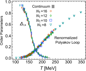
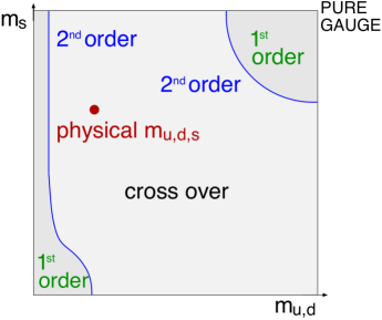
Figure 2.3: (Left) Subtracted and normalised chiral condensate, along with renormalised Polyakov loop (see [61] for precise definitions), in $2+1$ flavour LQCD simulation. Figure taken from [61], which was in turn adapted from [67]. $N_{t}$ is the lattice site number along the temporal direction. (Right) “Columbia plot”, taken from [62], generated from $2+1$ flavour LQCD simulation.

It is possible to formulate QCD non-perturbatively by discretising Euclidean spacetime on a lattice, giving rise to what is known as Lattice QCD (LQCD). Fig. 2.3 shows two plots with data from LQCD calculations, which are intended to shed some light on the phase transitions that we have been discussing. On the left, we have the two order parameters, corresponding to the chiral condensate and the Polyakov loop. The main feature of this plot that we wish to draw attention to is the fact that the curves intersect at a point where the chiral condensate (Polyakov loop) is steeply decreasing (increasing), implying that both crossovers (see below) occur at roughly the same temperature. This certainly does not provide a proof that the two crossovers occur at the same temperature in nature, since in reality, quarks cannot be considered infinitely heavy. Nevertheless, as we are not so concerned with the details of the crossover in what follows, we refer to both crossovers collectively in what follows as the QCD transition.

On the right of Fig. 2.3, we have what is known as a “Columbia plot”, with the name coming from the birthplace of the original paper [68]. These kinds of plots come from LQCD calculations where one can vary the number of flavours as well as the quark masses in order to investigate the role they play in observed phenomena. As is clearly visible, for physical values of the up, down and strange quarks, where the latter is much heavier than the former two (which are approximately equal) , the QCD transition exhibits a crossover. As opposed to a first or second-order phase transition, this implies that there is no order parameter, which diverges or jumps at the critical temperature. Looking to Fig. 2.2, we note the depiction of this crossover near the $\mu_{B}=0$ axis. Recent results produced from the HotQCD LQCD collaboration [69] with two degenerate up and down dynamical quarks and a dynamical strange quark give a pseudo-critical temperature of $T_{pc}=156.5\pm 1.5\text{MeV}$. One can see by eye that this is where the dotted curve intersects the temperature axis in Fig. 2.2.

While LQCD is an extremely useful tool for understanding the strong coupling regime of QCD, its use is somewhat limited to the $\mu_{B}=0$ axis due to the infamous sign problem [70]. The sign problem stems from the fact that, upon adding a chemical potential term to the discretised Euclidean path integral, one runs into the problem of complex probability measures, which are difficult to handle with numerical integration. At very small $\mu_{B}/T$, one can use various techniques [71, 72, 73, 74, 75] to track the QCD transition for non-zero values of $\mu_{B}$ but the accuracy of these methods deteriorates once $\mu_{B}/T$ becomes $\mathcal{O}(1)$.

Along with the extension of LQCD to non-zero $\mu_{B}$ mentioned above, one has to rely on holographic models (see footnote 21) or the Polyakov-extended Nambu-Jona-Lasino (PNJL) [76, 77] model to study the regime of larger $\mu_{B}$, which suggest that the nature of phase transition could be first-order in this region. If such a first order transition exists, one would expect this region to be connected to the crossover region by a critical point. A huge amount of experimental resources are currently being spent on trying to identify this critical point, in what are known as heavy-ion collisions. We will come back to this topic in the next section.

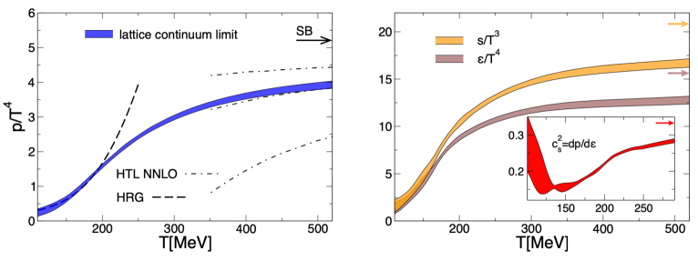
Figure 2.4: Continuum-extrapolated equation of state from $2+1$ flavour lattice simulations [78]. The left panel shows the pressure whereas the right shows the energy density, both suitably normalised. The insert on the right panel shows the speed of sounds. The arrows indicate the Stefan-Boltzmann limit for a non-interacting gas of massless quanta. HRG stands for hadron resonance gas and HTL for hard thermal loop. There is a large uncertainty associated with the HTL calculation, derived from the choice of renormalisation scale.

For large values of $T$ or $\mu_{B}$ (in the deconfined regime), one can take an analytic perturbative approach (to be introduced in Ch. 4). For large $T$ and small $\mu_{B}$ calculations from such an approach turn out to be consistent with LQCD results. In particular, looking to Fig. 2.4-left one can see a good agreement between the LQCD equation of state at high temperature and the perturbative (HTL) result. The large uncertainty there is associated with the choice of renormalisation scale, $\mu$, which agrees well with the lattice result for $\mu=2\pi T$. We furthermore note that the lattice result agrees well with the prediction from the hadron resonance gas model for lower temperatures, before it begins to diverge at $T\sim 150\text{MeV}$.

In contrast, for large $\mu_{B}$ and small $T$, a colour super-conducting phase is implied [79, 80, 81, 82]. There is an intense ongoing effort to understand whether this deconfined phase of quark matter is found in neutron star cores [83]. Such an effort has been boosted on the experimental side by the detection of gravitational waves from neutron star mergers by the LIGO and VIRGO collaborations [84, 85].

2.4 Heavy-Ion Collisions and the Quark-Gluon Plasma

In the previous section, we tried to give a relatively brief overview of the QCD phase diagram, picking out and discussing some of its defining features. If we keep increasing the temperature indefinitely, one expects from asymptotic freedom to find a weakly coupled plasma, where the fundamental degrees of freedom are quarks and gluons – the quark-gluon plasma (QGP). The term QGP was introduced in the early 1980s by Shuryak [86], by which point it had been realised that this state of matter should have existed in the very early universe, a few microseconds after the Big Bang. This realisation set off a coordinated effort to try and recreate the QGP in a laboratory setting, which in turn, prompted the colliding of heavy ions at several colliders, thereby giving birth to the notion of creating and probing the QGP in heavy-ion collisions (HIC). These days, the most energetic HIC take place at the LHC, where mainly Pb-Pb collisions are performed with centre of mass energy per nucleon, $\sqrt{s_{\text{NN}}}$ on the order of a few TeV. At RHIC, Au-Au and U-U collisions are instead performed going up to $\sqrt{s_{\text{NN}}}\approx 200\text{GeV}$. Extensions of this program to even lower energies are planned at the Japan Proton Accelerator Research Complex (J-PARC), the Facility for Antiproton and Ion Research (FAIR) in Darmstadt, Germany as well as the Nuclotron-based Ion Collider fAcility (NICA) in Dubna, Russia. The motivation for running less energetic HIC experiments is that it allows one to scan the QCD phase diagram across larger values of $\mu_{B}$, thus providing a systematic strategy for the search of the QCD critical point. A sketch of this is shown in Fig. 2.2.

2.4.1 Stages of a Heavy-Ion Collision

Can we say with some level of confidence whether or not the QGP is created in HIC? The answer is yes, but we refrain from diving further into this topic until after we lay out the different stages of the HIC, following mainly [88, 89, 63, 55].

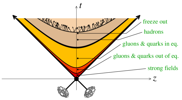
Figure 2.5: The main stages associated with a heavy-ion collision, as described in the main text. Figure taken from [63].

In HIC, the QGP is created and expands, primarily along the beam axis, which we identify as the $x^{1}$ direction. An idea originally proposed by Bjorken [90], says that such collisions, consisting of greatly Lorentz-contracted nuclei, are approximately independent of the spatial rapidity variable,

$$y\equiv\frac{1}{2}\ln\frac{x^{0}+x^{1}}{x^{0}-x^{1}}.$$ (2.19)

In this way, one is permitted to order the different stages of the collision in terms of
$\tau=\sqrt{({x^{0}})^{2}-({x^{1}})^{2}}$, the proper time of an observer comoving with a fluid element of the QGP. These hyperbolas, which can be identified as hypersurfaces of constant energy density are marked clearly in Fig. 2.5

1. $\tau=0\,\text{fm}/\text{c}$: The incoming Lorentz-contracted nuclei (in the laboratory frame), give rise to the typical picture of two colliding pancakes. These pancakes are composed mostly of gluons, carrying only tiny fractions $x\ll 1$ of the longitudinal momenta of their parent nucleons, albeit with a density that increases with $1/x$. By the uncertainty principle, such a high-density system can carry large amounts of transverse momentum. It turns out that this high-density gluonic form of matter dominates the hadron wavefunction at mid-rapidity and can be described using the Colour Glass Condensate (CGC) effective theory [91, 92]. See below Fig. 2.6 for a short elaboration.

   As the actual collision takes place, hard processes occur, i.e those where the outgoing particles possess large amount of transverse momenta, $Q$. Taking place over a timescale of $1/Q$, particles produced in hard collisions: jets (of light quarks), heavy quarks, vector bosons, photons and dileptons, bear witness to the entire HIC event and are often used to characterise the topology of the final state. We will come back to discuss some of these hard probes shortly.

   

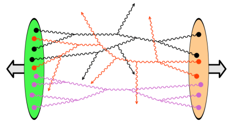
   Figure 2.6: Out-of-equilibrium gluons liberated by the nucleus-nucleus collision. Figure taken from [93]. In the Colour Glass Condensate (CGC) model, one assumes that the energy deposition is dominated by the liberation of gluons from the colliding nuclei and that the relevant gluon content can be described by semiclassical gauge fields. In such a description, the relevant information about an incoming nucleus is contained in the colour current it carries, which acts as a source for the colour field.

2. $\tau\sim 0.2\,\text{fm}/\text{c}$: The bulk of the partonic constituents of the colliding nuclei (the gluons making up the CGC) is liberated. Most of the hadronic content observed in the detectors stems from this liberation. Before hitting the detectors, these particles undergo a complex evolution, forming an out-of-equilibrium, dense medium, known as the glasma.

3. $\tau\sim 1\,\text{fm}/\text{c}$: If the produced partons did not interact with each other, or if they interacted weakly, they would independently evolve, racing towards the detectors. However, there is evidence that they in fact do interact strongly, exhibiting collective phenomena, which we come back to in Sec. 2.4.4. In particular, by $\tau\sim 1\,\text{fm}/\text{c}$ the partons are thought to have thermalised, giving rise to a (locally) equilibrated state of matter, the quark-gluon plasma. A microscopic description of this thermalisation is provided by bottom-up thermalisation [94, 95], where the harder gluons contained in the colliding nuclei radiate soft gluons. These soft gluons form a thermal bath that drains away energy from the harder gluons through elastic scattering (see Fig. 3.1-left), and radiation (see Fig. 3.1-right) thereby thermalising them.

4. $\tau\sim 10\,\text{fm}/\text{c}$: Upon its formation the QGP, continues to expand and cool. By this time, the local temperature decreases to that where the transition to a confined state lies ($T_{c}\sim 150\,\text{MeV}$) and the medium’s constituents begin to hadronise. This hadronic system is still relatively dense, so it preserves thermal equilibrium while expanding, inhabiting the hadron gas form of matter mentioned previously. At some point, the hadrons continue to interact with each other but only elastically, which is known as the chemical freeze-out.

5. $\tau\sim 20\,\text{fm}/\text{c}$: By this time, the density becomes so low that the hadrons no longer interact with each other at all, indicating the kinetic freeze-out. They then proceed to free-stream all the way to the detector.

In this thesis, we are primarily interested in the intermediate stage, where the QGP has equilibrated. Still, it is remarkable that all of the complexity, arising throughout the various stages above stems from the QCD Lagrangian, Eq. (2.10). With this picture in mind, we proceed to explore in more detail some of the various probes of the QGP, and how they can inform us further about its properties.

2.4.2 Jet Quenching

Note that up to this point, we have essentially assumed the presence of the QGP without providing any direct evidence for its existence. It was first proposed by Bjorken in the early 1980’s [3] that the presence of a QGP in high multiplicity hadron-hadron collisions would result in the suppression of high-$p_{T}$ jets. This sparked a great effort to try and observe this distorting or quenching of jets in HIC. The realisation of this goal arrived at RHIC in the early 2000’s [4, 5], where a suppression of the high $p_{T}$ spectra in central collisions was observed. A few years later, evidence towards the existence of jet quenching was further solidified at the LHC [96, 97] with fully reconstructed jets.

Based on our discussion in Sec. 2.2, it should not come as a surprise that jets serve as an ideal hard probe of the QGP. As objects created at the beginning of the collision in hard processes, they persist through all phases of the HIC and can be used as a differential tool to study the QGP across a multitude of scales.

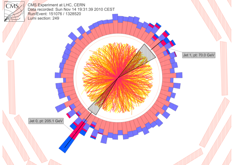
Figure 2.7: (Left) Event display showing dijet asymmetry in a $\text{Pb}+\text{Pb}$ collision at $\sqrt{s_{\text{NN}}}=2.76\,\,\text{TeV}$(CMS).

In the absence of a QGP, dijets, produced back-to-back are expected to propagate all the way to the detectors, registering (approximately) equal amounts of energy in the opposing calorimeters. Yet in HIC, it is possible that one of the dijets will pass through more of the QGP than the other and become quenched in comparison. This expectation seems to be realised in nature, based on what is shown in Fig. 2.7-left. In this context, the quenching can be quantified by the dijet asymmetry, $A_{J}=(p_{T\,1}-p_{T\,2})/(p_{T\,1}+p_{T\,2})$, where $p_{T\,1}$ ($p_{T\,2}$) is the transverse momentum of the reconstructed leading (sub-leading) jet.

In an ideal scenario, one would like to be able to compare what happens to a jet when it passes through the QGP to what happens when there is no QGP. This is what is roughly expected p-p collisions, which, as we mentioned in Sec. 2.2 are relatively well-understood. Indeed, to try and quantify the quenching in this way, one can use the nuclear modification factor [98], related to the ratio of the jet yield in HIC to the cross-section in $p-p$ collisions

$$R_{\text{AA}}=\frac{\frac{1}{N_{\text{evt}}}\frac{d^{2}N_{\text{jet}}}{dp_{T}dy}}{\langle T_{\text{AA}}\rangle\frac{d^{2}\sigma_{\text{jet}}}{dp_{T}dy}}$$ (2.20)

where $N_{\text{evt}}$ is the number of events, $T_{\text{AA}}$ the nuclear thickness function, which can be calculated using the Glauber model [99]. By taking such a ratio, one hopes that hadronisation effects in both kinds of collisions “cancel out”. In Fig. 2.8-left, $R_{\text{AA}}$ is plotted for several centrality classes in Pb-Pb collisions. $R_{\text{AA}}$ is less than unity for the entirety of the kinematic range and is even smaller in more central collisions, which is again consistent with Bjorken’s “jet extinction” hypothesis.

Indeed, $R_{\text{AA}}$ is not restricted to quantifying the relative suppression of jets – it can be defined analogously for other hard probes, a few of which will be mentioned in the next section. One issue with $R_{\text{AA}}$ is that depends somewhat on the underlying $p_{T}$ spectrum of the objects of interest; for fixed energy loss, a spectrum with steeper $p_{T}$ dependence will have a smaller $R_{\text{AA}}$ value. The recent reviews [101, 102] should be consulted for more information on this issue as well as the more general field of jet quenching phenomenology.

The message that we have tried to impart here is simply that experimental measurements have shown that jet quenching is realised at the LHC and RHIC. In Ch. 3, we will dive further into the theoretical side of jet energy loss, showing how one can quantify the quenching of a jet with some (relatively) simple analytical calculations.

2.4.3 Other Hard Probes

In Sec. 2.3, we mentioned that because of thermal screening, heavy quarks should not be able to form bound states, known as quarkonia, in the deconfined phase. Historically, this lead to the idea by Matsui and Satz [103] that quarkonia can be used as a “thermometer” for the medium: $\bar{Q}Q$ bound states formed in the initial stages of the HIC will begin to dissociate once the Debye screening length (to be discussed in Ch. 4) becomes shorter than the size associated with the bound state. Afterwards, the quark and antiquark should evolve independently in the medium until the plasma cools down to $\Lambda_{\text{QCD}}$, at which they bind with light quarks or antiquarks to form heavy-light mesons, leading to an overall suppression of quarkonia. There is an additional complication, namely that, charm quarks which are produceed in abundance in HIC may have a high enough density to then recombine at a later stage of the collision. See the recent reviews [104, 102] for more information.

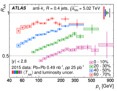
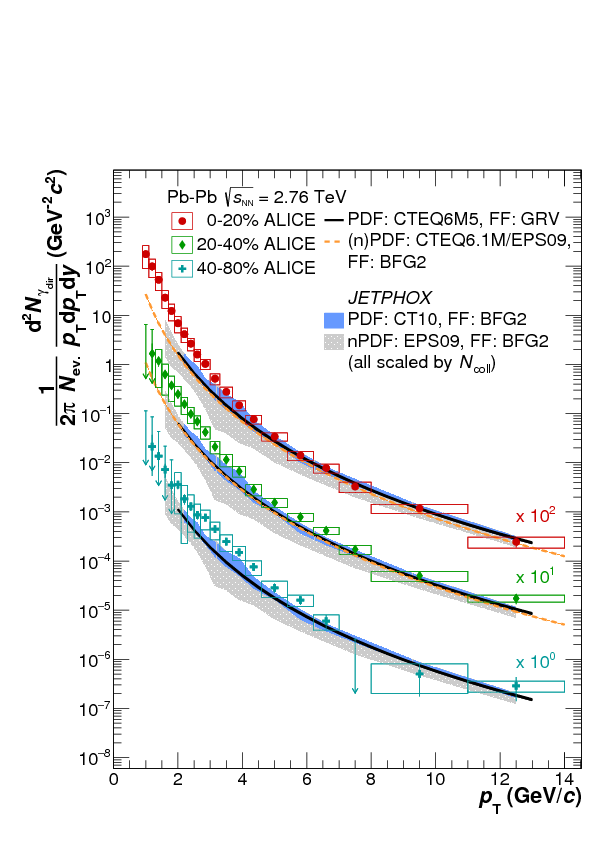
Figure 2.8: (Left) Nuclear modification factor plotted for a range of different centrality classes, taken from [105]. (Right) pQCD prediction of direct photon production compared with experimental results from the ALICE collaboration [106].

Electromagnetic radiation can also provide a window into the inner workings of the QGP, but in a somewhat different way to that of jets and heavy quarks. Since the mean free path of photons produced in the HIC is considerably larger than the size of the QGP, they never equilibrate with the medium. Coupled with the fact that neither photons nor the dilepton pairs they decay into hadronise, it is reasonable to assert that perturbative calculations may do a decent job of predicting photon and dilepton production. On the experimental side, an issue is that one has to work very hard to understand the origins of the electromagnetic radiation: there are direct photons, produced as a result of partonic interactions in addition to decay photons, which are produced from the decay of light hadrons. At the same time, the various forms of production allow one to use the observed spectrum to report on local conditions at the radiation’s creation point [107]. Indeed, Fig. 2.8-right shows very good agreement of an NLO pQCD calculation of the direct photon spectrum with experimental results from the ALICE collaboration. Moreover, the exponential shape of the spectrum suggests that these photons were emitted from a thermalised medium.

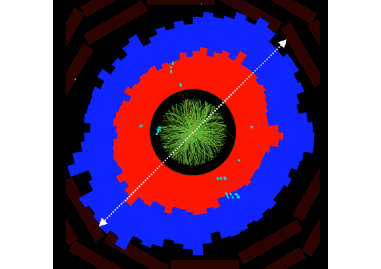
Figure 2.9: CMS event dispay, taken from [108]. The green lines are charged tracks and energy in the electromagnetic and hadronic are denoted by red and blue respectively. The dotted white line traversing the display highlights the final state anisotropies in the azimuthal direction.

2.4.4 Collective Flow

Up to this point, we have concentrated solely on hard probes of the QGP. That is not to say that the soft content produced in HIC cannot tell us anything about the medium. From Fig. 2.9, which shows the event display in the azimuthal plane, we note that the soft particles are not deposited uniformly throughout the detector: there is increased production along the dotted line. This conclusion can be reached in a more quantitative manner by looking at the distribution of particle pairs, differential in the azimuthal angle and rapidity between the two particles [109]. There, one observes a cosine modulation in the azimuthal direction, which implies a momentum anisotropy in the final state. This anisotropy is quantified by the so-called flow coefficients, $v_{n}$, defined as the Fourier coefficients of the azimuthal distribution of particles.

This phenomenon is particularly prominent in non-central collisions, where a relatively large impact parameter implies an almond-shaped overlap zone between colliding nuclei, generating increased pressure in the azimuthal direction, which gives rise to a spatial anisotopy in the initial state. Modelling the QGP as a fluid through the use of viscous hydrodynamics has proven extremely successful in showing how an initial state spatial anisotropy can give rise to final state momentum anisotropies [110, 111, 112, 113]. Moreover, in the hydrodynamical framework, where the medium’s properties are characterised by transport coefficients, one can reproduce values for the shear viscosity to entropy ratio, $\eta/s\sim 0.1-0.3$ that are consistent with those measured at the LHC and RHIC [114, 115, 116, 117, 118]. These values also happen to be reasonably close to $\eta/s=1/4\pi$, calculated using the strong-coupling technique, holography [119, 120, 121]. Strikingly, a small value for $\eta/s$ would imply that the QGP is so strongly coupled that very little (net) momentum can be transferred to nearby fluid elements. Moreover, such a value would imply that fluid cannot be described in terms of quasiparticles with mean free path: to do so, one would have to require mean free paths smaller than $1/T$. Perhaps unsurprisingly, calculations using finite-temperature perturbation theory [123, 124, 125] are not able to reproduce such a small value of $\eta/s$.

As an aside, we note that collective effects have recently been observed in “small systems”, namely p-p and p-Pb collisions [126], implying that a QGP may be formed in that case as well. So far however, there has been no signature of jet quenching in these collisions, implying that the pursuit of quantifying jet quenching by comparing to p-p collisions may not be such a hopeless one after all. See [127] for a recent review.

Getting back to the strong coupling discussion, it is fair to say that the success of viscous hydrodynamics to describe the QGP’s strongly coupled, collective behaviour sparked the increased employment of strong coupling techniques. The rest of this thesis will nevertheless be based on the utilisation finite-temperature perturbation theory, applied to jet quenching. We argue that such an endeavour is not a futile one for the following reasons:

• QCD perturbation theory, by definition maintains a strong connection with first principles and can sometimes provide analytical results where LQCD cannot. In the holographic setup, while analytical results can undoubtedly be obtained, the strongly coupled theory that one is studying is not QCD but rather $\mathcal{N}=4$ super Yang-Mills theory, a supersymmetric conformal theory. Therefore, holography is considered more as a guiding light, as opposed to a tool with which one can make concrete, observable predictions.

• Even if the QGP is strongly coupled, the jet itself is still weakly coupled. More precisely, if one wants to calculate the probability of a quark jet radiating a gluon, the factor of $\alpha_{s}$ associated with this probability should be much smaller than one, given the jet’s extremely large energy.

• In a strong coupling picture, interactions between the jet and QGP constituents will be characterised by a value of $\alpha_{s}$ which is not smaller than one. However, as we will see in Sec. 4.4.3 and Ch. 6, it is sometimes possible to evaluate thermal correlators on the lightcone using a certain resummation procedure, which thus provides a non-perturbative evaluation.

With these points in mind, we conclude this chapter and proceed to the next one, where we explore some parts of the jet energy loss literature.

Chapter 3 Jet Energy Loss

Given the large background present in HIC (looking again to Fig. 2.7), one immediately understands why it is extremely difficult to extract precise details of the QGP [136] from experiment. This means that on the theory side, it is imperative to have a quantitatively precise understanding of the jet-medium interaction. One of the purposes of this chapter is to review the progress made towards this pursuit. However, its primary goal is to provide the reader with a clear physical picture, which can be relied on throughout the rest of the thesis.

In Sec. 3.1 we discuss the different ways that the jet can interact with the medium through the lens of kinetic theory. In doing so, we understand that depending on the relevant region of phase space, bremsstrahlung can be triggered by multiple scatterings between the jet and medium constituents. To appropriate deal with such a region, one needs to take care of LPM interference and we sketch how this is done in Secs. 3.2 and  3.3. In Sec. 3.4, we diverge momentarily to discuss the transverse scattering kernel, an object, which controls how the jet diffuses in transverse momentum space before exploring another dominant region of phase space, the single-scattering regime in Sec. 3.5. Secs. 3.6 and  3.7 are then respectively devoted to giving a bird’s-eye view of the jet energy loss literature and a brief summary of some recent developments.

A word of caution is in order: in the previous chapter, it has been highlighted that jets are complicated objects and that Monte-Carlo methods are needed to simulate their full evolution. In what is to follow, however, the jet is interchangeably referred to as a single hard parton with initial four momentum $P=(E,0,0)$. By hard, we mean that $E\gg T$ with $T$ the temperature of the plasma. In this chapter, both the jet and its radiation (which is strictly speaking, also part of the jet) is assumed to be hard. We relax this latter assumption in Ch. 5. See App. A for conventions and notation.

3.1 Jet Quenching in Kinetic Theory

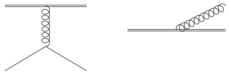
Figure 3.1: On the left, we have $2\rightarrow 2$ scattering, also known an elastic collision, with the bottom single line representing a medium quark or gluon. On the right, we have $1\rightarrow 2$ scattering or an inelastic collision. In both cases, the double line can be either a hard quark or a hard gluon. The hard partons are deliberately denoted by straight lines to emphasise their eikonal nature. As is true for all diagrams in this chapter, time flows from left to right.

Before embarking on the derivation of an actual energy loss calculation, we will classify the different kinds of collisions between the jet and medium and mention their relative impact on energy loss.

In the very same paper where Bjorken first proposed using jet quenching as a way to detect the presence of the QGP [3], he provided an estimate of collisional energy loss of a massless parton in colour representation $R$

$$\frac{dE}{dz}=C_{R}\pi\alpha_{s}^{2}T^{2}\left(1+\frac{N_{f}}{6}\right)\ln\frac{ET}{m_{D}^{2}}$$ (3.1)

per unit length, $z$ traversing a plasma of temperature, $T$. Collisional or elastic energy loss is classified as that which comes directly from $2\to 2$ scatterings between the jet and QGP constituents. A typical diagram contributing to collisional energy loss is depicted in Fig. 3.1-left. For the case of a hard, light parton, this form of energy loss is dominated by Coulomb scatterings. The argument of the logarithm is a ratio of the maximum possible momentum exchange between the jet with energy $E$ and medium constituent with energy $\sim T$ and the minimum possible momentum exchange, dictated by the Debye screening mass, $m_{D}$ [142, 143]. This result has since been built upon, taking into account finite size effects [144], considering heavy quarks [145] and the effect of Compton scattering [146]. See [147] for a review. We mention that for RHIC and LHC conditions, collisional energy loss on its own is expected to be negligible in comparison to radiative energy loss [148, 149], which we move on to discuss now.

In the early 2000’s, Arnold, Moore and Yaffe (AMY) developed an effective kinetic theory [123, 150, 151, 152, 153, 124] to study jet energy loss, centred around the Boltzmann equation

$$\bigg{(}\frac{\partial}{\partial t}+\vec{\mathbf{v}}\cdot\vec{\nabla}_{\vec{\mathbf{x}}}\bigg{)}f^{a}(\vec{\mathbf{p}},\vec{\mathbf{x}},t)=-C_{a}^{2\to 2}[f]-C_{a}^{1\to 2}[f],$$ (3.2)

where $f^{a}(\vec{\mathbf{p}},\vec{\mathbf{x}},t)$ is the classical phase space distribution for a single colour and helicity state quasiparticle. Roughly speaking, the Boltzmann equation describes how changes in the hard parton’s momentum, $\vec{\mathbf{p}}$ occur by loss or gain through scattering. The different kinds of scattering processes are then included through the collision operators on the right hand side; elastic collisions are incorporated through the operator $C_{a}^{2\to 2}[f]$. The second term $C_{a}^{1\to 2}[f]$, instead reflects the fact that the jet can also shed energy by splitting, be it through bremsstrahlung or pair production. A bremsstrahlung diagram is depicted in Fig. 3.1-right.

For on-shell particles in the vacuum, processes such as the one in Fig. 3.1-right are kinematically disallowed. However, when passing through the QGP, the hard parton may interact with the medium, exchanging a soft gluon (i.e through an elastic collision with momentum exchange $\sim gT$) and in doing so be pushed slightly off-shell. Upon picking up this small virtuality, the parton will then have the ability to radiate; it is for this reason that the operator $C_{a}^{1\to 2}[f]$ captures what is known as radiative or medium-induced energy loss.

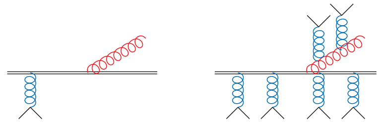
Figure 3.2: Single-scattering (left) and multiple scattering (right). Blue gluons are those that are exchanged in the jet-medium interaction whereas red gluons are medium induced radiation. In the multiple scattering regime, bremsstrahlung is unable to resolve individual elastic collisions, which is a manifestation of LPM interference.

It is not obvious why diagrams such as the one in Fig. 3.2-left contribute at the same order as the one in Fig. 3.1-left since the former possesses an extra factor of $g$. Nevertheless, it turns out that the contribution from these kinds of diagrams is enhanced when, looking to Fig. 3.2: the momentum exchanged with the medium, $K$ is spacelike and soft$\sim gT$. We will not wade through the details here but one can show [155, 150] that if these conditions are met, the propagators from the internal lines in Fig. 3.2 compensate for the extra factor of $g$ in the numerator of the same diagram, implying that radiative energy loss in at least as parametrically as important as collisional energy loss. Be that as it may, it transpires that in order to properly include these radiative scattering processes into the kinetic theory, one needs to overcome another major hurdle.

One of the assumptions tied to the validity of the Boltzmann equation Eq. (3.2) is that the de Broglie wavelength of the hard partons must be small compared to their mean free path. This allows one to treat the partons as classical particles between scatterings, meaning that $\vec{\mathbf{x}}$ and $\vec{\mathbf{p}}$ can be treated as classical variables in the Boltzmann equation. For a jet particle with energy $E\gg T$, its de Broglie wavelength is of course $\lambda\sim 1/E$. To see if this assumption holds here, let us estimate the cross-section of an elastic collision such as that in Fig. 3.1-left, with the exchanged momentum soft, $K\sim gT$. After squaring the amplitude and integrating over the final state phase space,

$$\sigma_{\text{el}}\sim\int d(K^{2})\bigg{|}\frac{g^{2}}{K^{2}}\bigg{|}^{2}\sim\frac{g^{2}}{T^{2}}.$$ (3.3)

The mean free path between collisions is then

$$l_{\text{el}}=\frac{1}{n\sigma_{\text{el}}}\sim\frac{1}{g^{2}T},$$ (3.4)

where we have used that the density of scatterers is $n\sim T^{3}$. Clearly, we have that $\lambda\ll l_{\text{el}}$ and we can conclude that this assumption is consistent with the framework of kinetic theory. Another requirement is that the quantum mechanical duration of individual scattering events be much smaller than the mean free time between collisions. If this condition is not satisfied, there will be quantum interference between successive scatterings, implying that they cannot be treated independently. The mean free time between elastic collisions is

$$t_{\text{el}}\sim\frac{1}{n\sigma_{\text{el}}v}\sim\frac{1}{g^{2}T}.$$ (3.5)

The scatterers are at rest with respect to the plasma frame so that we can set the relative velocity, $v\sim 1$. The scattering duration associated with these elastic collisions is instead

$$\tau_{\text{el}}\sim\frac{1}{K}\sim\frac{1}{gT},$$ (3.6)

implying that the aforementioned condition is indeed satisfied. Hence, the energy loss coming from the elastic collisions can be safely implemented in Eq. (3.2). But what about radiative energy loss?

Let us now go back to Fig. 3.2-left, specialising to the case of democratic $q\to qg$ splitting (so that we may estimate the energy of the radiation as $\sim E$). It turns out that the internal quark line will be pushed off-shell in energy by an amount

$$\delta E\sim\frac{Q_{\perp}^{2}}{E},$$ (3.7)

where $Q_{\perp}$ is the size of momentum transfer (transverse to the hard parton’s direction of motion) in the underlying scattering process. Fourier transforming, we can then identify the duration associated with the bremsstrahlung process as the formation time,

$$\tau\sim\frac{1}{\delta E}\sim\frac{E}{Q_{\perp}^{2}}.$$ (3.8)

$Q_{\perp}$ is bounded by below by $m_{D}\sim gT$ (see Sec. 3.4 for a justification). Depending on the values of $Q_{\perp}$ and $E$, one can have $\tau\ll t_{\text{el}}\sim 1/(g^{2}T)$, a region of phase space known as the single-scattering regime. In this region, one can really consider a single collision with the medium to trigger bremsstrahlung as in Fig. 3.2-left.

Be that as it may, as $E\to\infty$ we become sensitive to a region of phase space where the formation time becomes comparable or larger than the mean free time between elastic collisions. Consequently, successive elastic collisions can no longer be treated as quantum mechanically independent for the calculation of bremsstrahlung. In this region, $Q_{\perp}$ should be thought of as the size of the momentum transfer during the formation time, effectively coming from multiple collisions. This coherence effect was first investigated in the context of QED by Landau, Pomeranchuk and Migdal [156, 157, 158] and is known as LPM interference.

In practice, in order to correctly account for radiative energy loss in this region known as the multiple scattering regime, one needs to sum an infinite number of interference terms, which are composed of diagrams such as Fig. 3.2-right.

3.2 Radiation Rate in the Multiple Scattering Regime

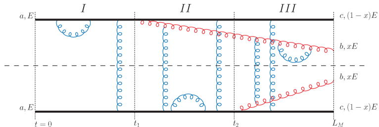
Figure 3.3: Interference terms contributing to the collinear splitting probability (see Eq (3.9)) of a hard quark, $a$ created at $t=0$ with initial energy $E\gg T$ radiating a gluon, $b$ with energy $\omega=xE$, before exiting the medium at $t=L_{M}$. The horizontal dashed line represents the cut between the amplitude above and the conjugate amplitude below. The upper and lower red curly lines are the radiated gluons in the amplitude and conjugate amplitude respectively. Exchanges of gluons with the medium are denoted by blue lines – these include both forward scatterings (loops) and true scatterings (vertical rungs), through which the initial or final state partons pick up transverse momentum kicks from the medium. It is assumed that all hard partons $a,b$ and $c$ propagate eikonally – this allows for a clean partitioning of the diagram into three regions, $I,II$ and $III$, separated by the hard, DGLAP vertices.
Figure reproduced from [159, 36].

In this section, we will demonstrate how the expression for the collinear radiation rate is obtained. The collinear radiation rate is a central ingredient within AMY’s kinetic theory formalism, originally produced through a strict diagrammatic derivation (within the context of photon production) in [150]. For the sake of brevity however, we choose to present here a formulation which resembles closer the work of Zakharov, while attempting to make contact with the AMY formalism along the way. The reason for insisting to maintain a connection with the AMY formalism (see Sec. 5.6.2) is that it is derived using Thermal Field Theory, to be discussed in some detail during the next chapter.

Before starting, we give the assumptions along with their justifications, while also making a point to state the simplifications that arise due to these assumptions:

• We require initial and final state partons propagate eikonally or in straight lines, with energies $\gg T$. This assumption allows us to neglect the presence of any statistical distribution functions (see Eqs. (4.23),  (4.27)), which are exponentially suppressed in this regime. Consequently, the partons probe the classical nature of the medium gauge field.

• The opening angle of the bremsstrahlung is small so that the emission itself can be described by the leading order DGLAP expressions [160]. Loop corrections to these vertices can then be neglected, provided that the factors of $g$ controlled by the transverse momentum picked up during bremsstrahlung formation time are also small. See Section VI. C of [161] for a discussion.

• The hard partons receive transverse momentum kicks through interactions which are instantaneous in comparison to the bremsstrahlung formation time. This is reasonable because the multiple scattering regime is dominated by soft collisions with a duration of order $\mathcal{O}(1/gT)$, whereas the mean free time between collisions is $\mathcal{O}(1/g^{2}T)$. We are then permitted to interpret time as flowing monotonically from left to right in Fig. 3.3, with the amplitude squared being cleanly separated into $3$ regions, defined by the radiation in the amplitude (region $II$) and the conjugate amplitude (region $III$). Since we are only interested in computing a radiation probability, which is not differential in transverse momentum, the system can then just be propagated through region $II$, since soft scatterings suffered by the partons in regions $I$ and $III$ will not contribute to LPM interference and thus need not be resummed. If one wants to remain differential in transverse momentum, a more sophisticated formalism [162, 163] is needed to account for regions $I$ and $III$.

• The medium is homogeneous in the transverse plane and static. These simplifications are of course difficult to justify making use of in a heavy-ion experiment. Nevertheless, improvements on these approximations will not impact our goal here, which is to demonstrate the application of the harmonic oscillator approximation.

Given these assumptions, we can then proceed, following [164, 159, 165, 166] to write down the differential splitting probability for a hard quark with initial energy $E$ to radiate a gluon with energy $\omega=xE$

$$\frac{dI}{d\omega}=\frac{2}{E}\text{Re}\bigg{\{}\frac{E}{2\pi V_{\perp}}\int_{t_{1}<t_{2}}dt_{1}dt_{2}\sum_{\text{pol.}}\int_{\mathbf{p}_{f},\mathbf{k}_{f}}\int_{\mathbf{p}_{1},\bar{\mathbf{p}}_{2},\mathbf{k}_{1}}$$

$$\times\bigg{\llangle}\Big{(}\langle\mathbf{p}_{f}\mathbf{k}_{f},t_{2}|\mathbf{p}_{1}\mathbf{k}_{1},t_{1}\rangle\langle\mathbf{p}_{1}\mathbf{k}_{1}|-i\delta H|\mathbf{p}_{i}\rangle\Big{)}\Big{(}\langle\mathbf{p}_{i},t_{1}|\bar{\mathbf{p}}_{2},t_{2}\rangle\langle\bar{\mathbf{p}}_{2}|i\delta H|\mathbf{p}_{f}\mathbf{k}_{f}\rangle\Big{)}\bigg{\rrangle}\bigg{\}}.$$ (3.9)

Let us take a moment to unpack the notation: $\mathbf{p}$ is transverse momentum of the hard quark and $\mathbf{k}$ the transverse momentum of the emitted gluon that splits with momentum fraction $x$. $\mathbf{p}_{i},\mathbf{p}_{f}$ denote the time momenta at time $t=1$ and $t=2$ respectively. The double-angled brackets $\llangle...\rrangle$ define a thermal average over the medium, composed of classical gauge fields, through which the partons propagate. The first set of round brackets on the second line contains the amplitude associated with the in-medium splitting process and the second set with the conjugate amplitude. Packed into these amplitudes are the collinear splitting matrix elements, i.e $\langle\mathbf{p}_{1}\mathbf{k}_{1},t_{1}|-i\delta H|\mathbf{p}_{i}\rangle$, where $\delta H$ is the part of the Hamiltonian containing the DGLAP vertices for the hard particles. In addition, there are the dressed propagators, such as $\langle\mathbf{p}_{f}\mathbf{k}_{f},t_{2}|\mathbf{p}_{1}\mathbf{k}_{1},t_{1}\rangle$, which resum multiple soft scatterings from the time of splitting in the amplitude, $t_{1}$ up until the time of splitting in the conjugate amplitude $t_{2}$. The sum is over the polarisation of the final state partons and the factors of $\frac{E}{2\pi}$ and $V_{\perp}$ are respectively artefacts of the normalisation of the initial state, $\langle\mathbf{p}_{i}|\mathbf{p}_{i}\rangle=V_{\perp}$ and having written $dk_{z}/2\pi=(E/2\pi)dx$. In equilibrium, the integrand can only depend on the difference between times, $t\equiv t_{2}-t_{1}$. We will nevertheless hold off on making this dependence explicit until later in the section.

We now move on to show how this two-particle, four-dimensional problem can be reduced to that of a one-particle, two-dimensional quantum mechanics problem. To start, let

$$\langle\mathbf{p}_{f}\mathbf{k}_{f},t_{2}|\mathbf{p}_{1}\mathbf{k}_{1},t_{1}\rangle =\langle\mathbf{p}_{f}\mathbf{k}_{f}|e^{-iH(t_{2}-t_{1})}|\mathbf{p}_{1}\mathbf{k}_{1}\rangle,$$ (3.10)

$$\langle\mathbf{p}_{i},t_{1}|\bar{\mathbf{p}}_{2},t_{2}\rangle =\langle\mathbf{p}_{i}|e^{iH_{*}(t_{2}-t_{1})}|\bar{\mathbf{p}}_{2}\rangle.$$ (3.11)

$H$ propagates the quark and gluon through the medium in the amplitude, along with $H_{*}$, which propagates the quark through the medium in the conjugate amplitude. The medium average in Eq (3.9) need then only be restricted to the factors depending on this part of the Hamiltonian, i.e

$$\bigg{\llangle}e^{-iH(t_{2}-t_{1})}|\mathbf{p}_{1}\mathbf{k}_{1}\rangle\langle\mathbf{p}_{i}|e^{iH_{*}(t_{2}-t_{1})}\bigg{\rrangle}.$$ (3.12)

Written like this, we can think of the object, $|\mathbf{p}_{1}\mathbf{k}_{1}\rangle\langle\mathbf{p}_{i}|$ as living in the Hilbert space

$$\bar{\mathbb{H}}_{\mathrm{q}}\otimes\mathbb{H}_{\mathrm{q,g}}=\bar{\mathbb{H}}_{\mathrm{q}}\otimes{\mathbb{H}}_{\mathrm{q}}\otimes\mathbb{H}_{\mathrm{g}},$$ (3.13)

with $\mathbb{H}_{\mathrm{q}}$ the Hilbert space of states of hard quark and $\mathbb{H}_{\mathrm{q,g}}$ the Hilbert space of states with a collinear quark-gluon pair. One then interprets this product rather as a Fock space of three particles: one quark, one gluon and one conjugate quark so that we may instead write

$$\bigg{\llangle}e^{-i(H-H_{*})(t_{2}-t_{1})}|\mathbf{p}_{a},\mathbf{p}_{b},\mathbf{p}_{c}\rangle\bigg{\rrangle}=e^{-i\mathcal{H}(t_{2}-t_{1})}|\mathbf{p}_{a},\mathbf{p}_{b},\mathbf{p}_{c}\rangle$$ (3.14)

with

$$(\mathbf{p}_{a},\mathbf{p}_{b},\mathbf{p}_{c}) =(-\mathbf{p}_{i},\mathbf{k}_{1},\mathbf{p}_{1})\quad\quad\quad\mathrm{at}\quad t=t_{1},$$ (3.15)

$$\mathbf{p}_{a}+ \mathbf{p}_{b}+\mathbf{p}_{c}=0.$$ (3.16)

The effective light-cone Hamiltonian is given as

$$\mathcal{H}=\delta E+ V(\mathbf{b}_{a},\mathbf{b}_{b},\mathbf{b}_{c})$$ (3.17)

$$\mathcal{H}=\varepsilon_{P_{b}}+ \varepsilon_{P_{c}}-\varepsilon_{P_{a}}+V(\mathbf{b}_{a},\mathbf{b}_{b},\mathbf{b}_{c}),$$

$$\varepsilon_{P_{j}}=\sqrt{p_{j}^{2}+m^{2}_{\infty j}},$$ (3.18)

with the $\mathbf{b}_{i}$’s transverse positions, conjugate to the $\mathbf{p}_{i}$’s. In the eikonal limit, where most of the particles’ momentum is carried by their $+$ components, the kinetic terms simplify to

$$\mathcal{H}=\frac{\mathbf{p}^{2}_{a}+m^{2}_{\infty a}}{2p^{+}_{a}}+ \frac{\mathbf{p}^{2}_{b}+m^{2}_{\infty b}}{2p^{+}_{b}}+\frac{\mathbf{p}^{2}_{c}+m^{2}_{\infty c}}{2p^{+}_{c}}+V(\mathbf{b}_{a},\mathbf{b}_{b},\mathbf{b}_{c}).$$ (3.19)

$$(p_{a}^{+},p_{b}^{+},p_{c}^{+}) =E(x_{a},x_{b},x_{c})=E(-1,x,1-x)$$ (3.20)

where the $m_{\infty i}$’s represent the asymptotic or in-medium masses.

The potential, $V(\mathbf{b}_{a},\mathbf{b}_{b},\mathbf{b}_{c})$ for the case of $q\rightarrow qg$ splitting is given as

$$V(\mathbf{b}_{a},\mathbf{b}_{b},\mathbf{b}_{c}) =-\frac{i}{2C_{F}}\Big{\{}\left(2C_{F}-C_{A}\right)\mathcal{C}_{F}(\mathbf{b}_{b}-\mathbf{b}_{a})$$

$$+C_{A}\mathcal{C}_{F}(\mathbf{b}_{c}-\mathbf{b}_{b})+C_{A}\mathcal{C}_{F}(\mathbf{b}_{a}-\mathbf{b}_{c})\Big{\}},$$ (3.21)

$$\mathcal{C}_{R}(\mathbf{b}) \equiv\int_{\mathbf{q}}\mathcal{C}_{R}(q_{\perp})(1-e^{i\mathbf{b}\cdot\mathbf{q}}).$$ (3.22)

We pause here to make some comments on the potential above:

• It is assumed that the potential takes this dipole-factorised form, with each term containing only depending on the difference of two transverse positions. This assumption holds up to at least NLO [11], where the threepole contributions have been shown to vanish.

• The potential is evidently imaginary as it describes the transverse momentum damping of a hard parton through its interactions with the medium. This of course implies that $\mathcal{H}$ is not Hermitian.

• The factor of $g^{2}$ appearing at the beginning of Eq. (3.21) characterises the strength of the interaction between partons and the medium and so the relevant scale for its running can be as low as that of the Debye mass [167].

• $\mathcal{C}_{R}(q_{\perp})$ is the transverse scattering kernel, related in the eikonal limit to the transverse scattering rate,

  $$\lim_{p^{+}\to\infty}\frac{d\Gamma_{R}(\mathbf{p},\mathbf{p}+\mathbf{q})}{d^{2}q_{\perp}}=\frac{\mathcal{C}_{R}(q_{\perp})}{(2\pi)^{2}}.$$ (3.23)

  for a high-energy parton in colour representation $R$. In an abuse of terminology, we refer to $\mathcal{C}_{R}(q_{\perp})_{R}$ interchangeably as the transverse scattering rate and the transverse scattering kernel in what follows. In the multiple scattering regime, with $q_{\perp}\gtrsim gT$ the appropriate scattering kernel can be computed using Hard Thermal Loop (HTL) effective theory [168],

  $$\mathcal{C}_{R}(q_{\perp})_{\text{HTL}}\equiv\frac{g^{2}C_{R}Tm_{D}^{2}}{q_{\perp}^{2}(q_{\perp}^{2}+m_{D}^{2})}.$$ (3.24)

  We will come back to discuss the scattering kernel further at a later point (see Sec. 3.4).

• Looking back to Fig. 3.3 can help us further understand how to interpret the different terms in $\mathcal{C}_{F}(\mathbf{b})$: the first one captures the correlations between the amplitude and itself or the conjugate amplitude and itself whereas the second term corresponds to background field correlations between the amplitude and the conjugate amplitude, separated by the transverse vector $\mathbf{b}$.

A further reduction of the dimensionality comes from the observation that there is an inherent symmetry with respect to how we choose the axis of jet propagation; it is possible to choose the $z$ axis to point in a slightly different direction while still maintaining the collinear approximations that we have made. Consequently, the splitting rate that we are deriving should be invariant under the transformations

$$(\mathbf{p}_{i},p_{i\,z})\rightarrow(\mathbf{p}_{i}+p_{i\,z}\mathbf{\xi},p_{i\,z}).$$ (3.25)

Since $p^{+}_{i}=x_{i}E$ and because of the zero sum of the $x_{i}$ and the $\mathbf{p}_{i}$, a single independent combination emerges

$$\mathbf{h}\equiv x_{b}^{+}\mathbf{p}_{a}-x_{a}^{+}\mathbf{p}_{b}=x_{c}^{+}\mathbf{p}_{b}-x_{b}^{+}\mathbf{p}_{c}=x_{a}^{+}\mathbf{p}_{c}-x_{c}^{+}\mathbf{p}_{a},$$ (3.26)

which is invariant under the aforementioned set of transformations. The kinetic part of the Hamiltonian, $\delta E$ in Eq (3.19) then reduces to

$$\delta E=-\frac{h^{2}}{2Ex_{a}^{+}x_{b}^{+}x_{c}^{+}}+\sum_{i=a}^{c}\frac{m_{\infty\,i}^{2}}{2Ex_{i}^{+}}$$ (3.27)

This reduction will also allow us to rewrite the potential in Eq. (3.19) by introducing the corresponding position variable

$$\mathbf{B}\equiv\frac{\mathbf{b}_{a}-\mathbf{b}_{b}}{x^{+}_{a}+x^{+}_{b}}=\frac{\mathbf{b}_{b}-\mathbf{b}_{c}}{x^{+}_{b}+x^{+}_{c}}=\frac{\mathbf{b}_{c}-\mathbf{b}_{a}}{x^{+}_{c}+x^{+}_{a}}$$ (3.28)

All together, the effective Hamiltonian then reads

$$\mathcal{H} =-\frac{h^{2}}{2Ex_{a}^{+}x_{b}^{+}x_{c}^{+}}+\sum_{i=a}^{c}\frac{m_{\infty\,i}^{2}}{2Ex^{+}_{i}}-\frac{i}{2C_{F}}\Big{\{}\left(2C_{F}-C_{A}\right)\mathcal{C}_{F}(-(x^{+}_{a}+x^{+}_{b})\mathbf{B})$$

$$+C_{A}\mathcal{C}_{F}(-(x_{b}^{+}+x_{c}^{+})\mathbf{B})+C_{A}\mathcal{C}_{F}(-(x_{c}^{+}+x_{a}^{+})\mathbf{B})\Big{\}}$$ (3.29)

We can now return to Eq. (3.9), and rewrite everything in terms of the momentum, $\mathbf{h}$, while also unpacking the hard vertices

$$\frac{dI}{d\omega}=\frac{\alpha_{s}P_{q\to qg}(x)}{x^{2}(1-x)^{2}E^{3}}2\text{Re}\int_{t_{1}<t_{2}}dt_{1}dt_{2}\int_{\mathbf{h}_{2},\mathbf{h}_{1}}\mathbf{h}_{2}\cdot\mathbf{h}_{1}\langle\mathbf{h}_{2},t_{2}|\mathbf{h}_{1},t_{1}\rangle.$$ (3.30)

$P_{q\to qg}(x)$ is the standard spin-averaged DGLAP splitting function for a $q\to qg$ splitting [160]. It reads

$$P_{q\to qg}(x)=C_{F}\frac{1+(1-x)^{2}}{x}.$$ (3.31)

Eq. (3.30) makes manifest the reduction to a 1-particle quantum mechanics problem. We are now going to try and make contact with the AMY formalism. Fourier transforming to $\mathbf{B}$ space

$$\frac{dI}{d\omega}=\frac{\alpha_{s}P_{q\to qg}(x)}{x^{2}(1-x)^{2}E^{3}}\text{Re}\int_{t_{1}<t_{2}}dt_{1}dt_{2}\mathbf{\nabla}_{\mathbf{B}_{2}}\cdot\mathbf{\nabla}_{\mathbf{B}_{1}}\langle\mathbf{B}_{2},t_{2}|\mathbf{B}_{1},t_{1}\rangle\Big{|}_{\mathbf{B}_{2}=\mathbf{B}_{1}=0}.$$ (3.32)

In equilibrium, the propagators only depend on the difference of times. Upon changing integration variables from $\{t_{1},t_{2}\}\to\{t_{1},t\}$, we then see that the entire integrand only depends on $t$. By differentiating with respect to $t_{1}$, we can then obtain an expression for the rate

$$\frac{d\Gamma}{d\omega}=\frac{\alpha_{s}P_{q\to qg}(x)}{x^{2}(1-x)^{2}E^{3}}\text{Re}\int_{0}^{\infty}dt\mathbf{\nabla}_{\mathbf{B}_{2}}\cdot\mathbf{\nabla}_{\mathbf{B}_{1}}\langle\mathbf{B}_{2},t|\mathbf{B}_{1},0\rangle\Big{|}_{\mathbf{B}_{2}=\mathbf{B}_{1}=0},$$ (3.33)

where the $t$ is now the time between the emission vertices in the amplitude and the conjugate amplitude. In integrating $t$ up to infinity, we are assuming the medium to have infinite length, in line with the AMY formalism. We specify that $\langle\mathbf{B}_{2},t_{2}|\mathbf{B}_{1},t_{1}\rangle$ is a Green’s function of the Schrödinger equation defined in Eq. (3.29), i.e

$$i\partial_{t}\Psi(\mathbf{B},t)=\mathcal{H}\Psi(\mathbf{B},t)$$ (3.34)

with initial condition

$$\langle\mathbf{B}_{2},t_{1}|\mathbf{B}_{1},t_{1}\rangle=\delta^{2}(\mathbf{B}_{1}-\mathbf{B}_{1}).$$ (3.35)

Then, we define

$$\mathbf{F}(\mathbf{B},t)\equiv 2i\mathbf{\nabla}_{\mathbf{B}_{1}}\langle\mathbf{B},t|\mathbf{B}_{1},0\rangle\Big{|}_{\mathbf{B}_{1}=0}.$$ (3.36)

This quantity obeys the same Schrödinger equation Eq. (3.34) as $\langle\mathbf{B}_{2},t|\mathbf{B}_{1},0\rangle$, i.e

$$i\partial_{t}\mathbf{F}(\mathbf{B},t)=\mathcal{H}\mathbf{F}(\mathbf{B},t),$$ (3.37)

albeit with an altered initial condition

$$\mathbf{F}(\mathbf{B},0)=-2i\mathbf{\nabla}_{\mathbf{B}}\delta^{2}(\mathbf{B}).$$ (3.38)

We then integrate Eq. (3.37) over time, using that $\mathbf{F}(\mathbf{B},t)$ decays as $t\to\infty$ because of the imaginary potential, which leaves us with

$$-2\mathbf{\nabla}_{\mathbf{B}}\delta^{2}(\mathbf{B})=\mathcal{H}\mathbf{F}(\mathbf{B}),$$ (3.39)

where we have defined the time-integrated amplitude

$$\mathbf{F}(\mathbf{B})\equiv\int_{0}^{\infty}dt\mathbf{F}(\mathbf{B},t).$$ (3.40)

Fourier transforming Eq. (3.39) back to $\mathbf{h}$ space, while using the explicit form of the effective Hamiltonian, Eq. (3.29) then yields

$$2\mathbf{h} =i\delta E\mathbf{F}(\mathbf{h})+\frac{1}{2C_{F}}\int_{\mathbf{q}}\mathcal{C}_{F}(q_{\perp})\bigg{\{}(2C_{F}-C_{A})[\mathbf{F}(\mathbf{h})-\mathbf{F}(\mathbf{h}-x\mathbf{q_{\perp}})]$$

$$+C_{A}[\mathbf{F}(\mathbf{h})-\mathbf{F}(\mathbf{h}+\mathbf{q_{\perp}})]+C_{A}[\mathbf{F}(\mathbf{h})-\mathbf{F}(\mathbf{h}-(1-x)\mathbf{q_{\perp}})]\bigg{\}}.$$ (3.41)

In addition, we can now rewrite Eq. (3.30) in terms of $\mathbf{F}(\mathbf{h})$ which now reads

$$\frac{d\Gamma}{d\omega}=\frac{\alpha_{s}P_{q\to qg}(x)}{4x^{2}(1-x)^{2}E^{3}}\int_{\mathbf{h}}\mathrm{Re}[2\mathbf{h}\cdot\mathbf{F}(\mathbf{h})].$$ (3.42)

Let us pause for a moment to recap. We have set out to compute the radiation rate of a hard quark traversing a weakly coupled QGP, while correctly taking into account LPM interference. The latter goal is explicitly realised through Eq. (3.41), which resums multiple scatterings between the hard partons and the medium. Its solution, $\mathbf{F}(\mathbf{h})$ is then fed into Eq. (3.30) thereby determining the rate, $d\Gamma/d\omega$.

3.3 The Harmonic Oscillator Approximation

We now proceed to introduce the Harmonic Oscillator Approximation (HOA) within the setup that has been put forward in the previous section. Our motivation for doing so is two-fold: on one hand, it will allow us to relatively easily obtain a well-known analytical result from the literature. Perhaps more importantly, it will give us an opportunity to clearly and precisely state the assumptions tied to the HOA, hence simultaneously determining the region of phase space in which it can be safely applied.

Before going on to solve Eq. (3.41) in the HOA, it will be useful to first define $\hat{q}_{R}(\mu_{\perp})$, the transverse momentum broadening coefficient

$$\hat{q}_{R}(\mu_{\perp})\equiv\int^{\mu_{\perp}}\frac{d^{2}q_{\perp}}{(2\pi)^{2}}q_{\perp}^{2}\mathcal{C}_{R}(q_{\perp}).$$ (3.43)

While it will soon be clear how $\hat{q}_{R}(\mu_{\perp})$ is related to the problem at hand, for the moment let us consider it as a transport coefficient, describing the hard parton’s diffusion in transverse momentum space. Asymptotic freedom should render the integral above UV finite. However, we would then be including harder, so-called Molière scattering [169, 170], which gives rise to two hard partons in the final state and is of course not a diffusive process. It is for this reason that $\hat{q}$ comes equipped with a UV cutoff, $\mu_{\perp}$.

$\hat{q}_{R}(\mu_{\perp})$ visibly depends on the transverse scattering kernel $\mathcal{C}_{F}(q_{\perp})$, which we take here to be the HTL kernel, defined in Eq. (3.24). Let us now go back to Eq. (3.41) and note that the $\mathbf{q}$ integration is logarithmically enhanced when:

• $h\sim Q_{\perp}\gg q_{\perp}$ with $Q_{\perp}$ the total momentum exchanged between the medium and parton during gluon emission. In other words, the momentum exchanged between the medium and parton during each collision should be much smaller than the total momentum exchanged during the formation time associated with the bremsstrahlung. We can then expand all of the $\mathbf{F}(\mathbf{h},x,\mathbf{q})$’s in Eq. (3.41) around $\mathbf{F}(\mathbf{h})$.

• $Q_{\perp}\gg m_{D}\sim gT$, so that the resulting logarithm can be considered large. One can then justify solving Eq. (3.41) to leading log (LL) accuracy, meaning that no effort is made to determine the constant under the logarithm. The solution to Eq. (3.41) to NLL accuracy has been obtained in [161].

If both of these criteria are satisfied, all of the mass terms will drop out of Eq. (3.27), since $m_{\infty}\sim gT$ at LO. The expansion then leaves us with a much-simplified form of Eq. (3.41)

$$2\mathbf{h}\approx i\frac{h^{2}}{2Ex(1-x)}\mathbf{F}(\mathbf{h})-\frac{C_{A}x^{2}+(2C_{F}-C_{A})+C_{A}(1-x)^{2}}{2}\int_{\mathbf{q}}\mathcal{C}_{F}(q_{\perp})\frac{q_{\perp}^{2}}{4}\nabla^{2}\mathbf{F}(\mathbf{h}).$$ (3.44)

At this point, we can then use Eq. (3.43) to write

$$2\mathbf{h}\approx i\frac{h^{2}}{2Ex(1-x)}\mathbf{F}(\mathbf{h})-\frac{C_{A}x^{2}+(2C_{F}-C_{A})+C_{A}(1-x)^{2}}{2C_{F}}\frac{\hat{q}_{F}(\mu_{\perp})}{4}\nabla^{2}\mathbf{F}(\mathbf{h}).$$ (3.45)

where

$$\hat{q}_{R}(\mu_{\perp})=\frac{g^{2}C_{R}Tm_{D}^{2}}{4\pi}\ln\frac{\mu_{\perp}^{2}}{m_{D}^{2}}$$ (3.46)

to leading log (LL) accuracy. By LL accuracy, we mean that there has been no attempt made to determine the constant under the logarithm. The logarithmic sensitivity on $\mu_{\perp}$ signals a contribution at the same order and with an opposite IR log divergence from the region $h\sim Q_{\perp}\sim q_{\perp}$. In this region, a single, harder scattering between the medium and the parton is responsible for the momentum exchanged, $Q_{\perp}$ during the formation time. In taking the HOA, this region is ignored, treating $\hat{q}_{R}(\mu_{\perp})$ itself as a parameter as opposed to some UV-regulated quantity. We call this parameter $\hat{q}_{0R}$. Continuing in this manner, we get

$$2\mathbf{h}=i\frac{h^{2}}{2Ex(1-x)}\mathbf{F}(\mathbf{h})-\frac{C_{A}x^{2}+(2C_{F}-C_{A})+C_{A}(1-x)^{2}}{2C_{F}}\frac{\hat{q}_{0F}}{4}\nabla^{2}\mathbf{F}(\mathbf{h}).$$ (3.47)

By rotational invariance $\mathbf{F}(\mathbf{h})\equiv\mathbf{h}\mathrm{F}(h^{2})$ and thus

$$2=i\frac{h^{2}}{2Ex(1-x)}\mathrm{F}(h)-\frac{C_{A}x^{2}+(2C_{F}-C_{A})+C_{A}(1-x)^{2}}{2C_{F}}\frac{\hat{q}_{0F}}{4}\left(\mathrm{F}^{\prime\prime}(h)+3\frac{\mathrm{F}^{\prime}(h)}{h}\right).$$ (3.48)

This equation can be solved by applying the boundary conditions that $\mathbf{F}(\mathbf{h})$ remain finite as $h\to 0$ and as $h\to\infty$

$$\mathbf{F}(\mathbf{h}) =\frac{4iEx(1-x)}{h^{2}}\left(\exp\left(-\frac{(\frac{1}{2}+\frac{i}{2})h^{2}}{H}\right)-1\right)\mathbf{h},$$ (3.49)

$$H \equiv\Big{(}Ex(1-x)(1-\frac{C_{A}}{C_{F}}x(1-x))\hat{q}_{0R}\Big{)}^{\frac{1}{2}}.$$ (3.50)

In order to get the rate, we need to extract the real part of $\mathbf{F}(\mathbf{h})$ and compute

$$\int_{\mathbf{h}}2\mathbf{h}\cdot\mathrm{Re}\,\mathbf{F}(\mathbf{h}) =\int_{\mathbf{h}}2(\mathbf{h}\cdot\mathbf{h})\frac{4Ex(1-x)}{h^{2}}\exp\left(\frac{-h^{2}}{2H}\right)\sin\left(\frac{h^{2}}{2H}\right)$$ (3.51)

$$=\frac{2Ex(1-x)H}{\pi}.$$ (3.52)

Plugging this back into Eq. (3.42), we get a result for the rate

$$\frac{d\Gamma}{d\omega}^{\text{LPM}} =\frac{g^{2}C_{F}}{8\pi E^{3}}\frac{1+(1-x)^{2}}{x^{3}(1-x)^{2}}\frac{Ex(1-x)\Big{(}Ex(1-x)(q-\frac{C_{A}}{C_{F}}x(1-x))\hat{q}_{0F}\Big{)}^{\frac{1}{2}}}{\pi}$$

$$=\frac{g^{2}C_{F}}{8\pi^{2}}\frac{1+(1-x)^{2}}{x^{2}(1-x)}\sqrt{\frac{x(1-x)(1+\frac{C_{A}}{C_{F}}x(1-x))\hat{q}_{0F}}{E^{3}}}.$$ (3.53)

Within the AMY framework this collinear rate is then fed into the term with the collision operator $C^{1\to 2}[f]$ on the right hand side of Eq. (3.2) along with the $g\to gg$ and $g\to q\bar{q}$ rates, after which point one can go and solve the (linearised) Boltzmann equation. Comparison with experimental data can be performed through, for instance, the embedding of these rates in the MARTINI event generator [171, 172].

In deriving Eq. (3.53), we have sketched a calculation of the collinear radiation rate, while showing how to properly account for LPM interference, as is necessary in the multiple scattering regime. Furthermore, we have showed how one can use the HOA in order to obtain an analytical solution in this regime. In what follows, we will demonstrate how this result fits within the context of the rest of the radiative jet energy loss literature. Before doing so, however, we will take a moment to clarify some of the details regarding the transverse scattering kernel, $\mathcal{C}_{F}(q_{\perp})$, which in principle depends on the model of the medium, as well as the scale of the transverse momentum exchanges between the jet and the QGP.

3.4 Choice of $\mathcal{C}_{F}(q_{\perp})$

As was already mentioned, the HTL kernel was used in the calculation of the quark collinear radiation rate, Eq. (3.53). In the context of this thesis, where we are using finite temperature perturbation to study what we call a weakly coupled QGP, it is the obvious choice. Yet, in the previous section, where we computed the radiation rate to LL accuracy, we never actually used the explicit form of Eq. (3.24). Rather, we just made use of the fact that upon plugging the HTL kernel in the integral equation, Eq. (3.41) the $q_{\perp}$ integration (in the multiple scattering regime) gives rise to a (large) logarithm.

In terms of calculating the collinear radiation rate to LL accuracy, we could have just as well used another kernel, originally proposed by Gyulassy and Wang (GW) [173]

$$\mathcal{C}_{R}(q_{\perp})_{\text{GW}}\equiv\frac{g^{4}C_{R}n}{(q_{\perp}^{2}+m_{D}^{2})^{2}},$$ (3.54)

where $n$ is the density of scattering centres. Instead of considering the medium to be weakly coupled, the GW kernel comes from modelling the medium as an ensemble of static scattering centres with Yukawa-like potentials.

In the case of the GW model, only static colour-electric fields are screened, whereas for the HTL kernel, since the colour charges are considered to be dynamical, both colour-electric and colour-magnetic fields need to be screened. However, the details with regard to screening are irrelevant at LL accuracy, precisely because this is the limit in which $q_{\perp}\gg m_{D}$. At NLL accuracy, individual momentum transfers of $q_{\perp}$ of order $m_{D}$ become important [161], in which case there is a difference between a full treatment of plasma screening and the static approximation.

Returning to the setting of a weakly coupled plasma, we remark that the HTL kernel should only be used for momenta $T\gg q_{\perp}$. For larger momentum exchanges $\sqrt{ET}\gg q_{\perp}\gtrsim T$, the appropriate kernel is

$$\mathcal{C}_{R}(q_{\perp})_{\text{hard}}=\frac{2g^{4}C_{R}}{q_{\perp}^{4}}\int_{l}\frac{l-l_{z}}{l}[C_{A}n_{B}(l)(1+n_{B}(l^{\prime}))+2N_{f}T_{F}n_{F}(l)(1-n_{F}(l^{\prime}))],$$ (3.55)

where $l^{\prime}=l+\frac{l_{\perp}^{2}+2\mathbf{l}\cdot\mathbf{q}}{2(l-l_{z})}$. For a kernel that interpolates between $\mathcal{C}_{F}(q_{\perp})_{\text{HTL}}$ and $\mathcal{C}_{F}(q_{\perp})_{\text{hard}}$, one can use [174, 18]

$$\mathcal{C}_{R}(q_{\perp})_{\text{smooth}}^{\mathrm{LO}}=\frac{2g^{4}C_{R}}{q_{\perp}^{2}(q_{\perp}^{2}+m_{D}^{2})}\int_{l}\frac{l-l_{z}}{l}\Big{[}C_{A}\,n_{\text{B}}(l)(1+n_{\text{B}}(l^{\prime}))+2N_{f}T_{F}\,n_{\text{F}}(l)(1-n_{\text{F}}(l^{\prime}))\Big{]}.$$ (3.56)

When $\mu_{\perp}\gg T$, the value for $\hat{q}_{R}(\mu_{\perp})$ reads

$$\hat{q}_{R}(\mu_{\perp}\gg T)=\frac{g^{4}C_{R}\xi(3)T^{3}m_{D}^{2}}{\pi}[2C_{A}+3N_{f}T_{F}]\ln\frac{\mu_{\perp}^{2}}{T^{2}},$$ (3.57)

which also includes a subleading $\ln T/m_{\text{D}}$ contribution not shown here. The ratio of the two leading log coefficients, (that is, comparing Eqs. 3.46 and  (3.57)) is $4\alpha_{s}T^{2}\xi(3)[2C_{A}+3N_{f}T_{F}]/(\pi m_{D}^{2})\sim 0.85$ for $N_{c}=N_{f}=3$ QCD.

We emphasise that everything discussed above applies to the restriction $q_{\perp}\gtrsim m_{D}$; the most frequent scatterings have momentum $m_{D}\gg q_{\perp}\gtrsim g^{2}T$ and are mediated by the exchange of low-frequency magnetic gluons. These interactions are not cut off by Debye screening but instead by non-perturbative effects [175]. That being said, they will not contribute to $\hat{q}_{R}(\mu_{\perp})$ and hence the radiation rate at leading order because of the extra factor of $q_{\perp}^{2}$ in the numerator of Eq. (3.43). As was mentioned in the previous chapter, the contribution of these low-frequency exchanges has been incorporated through the Lattice EQCD calculation [15, 13], to be discussed in Sec. 4.4.3.

3.5 Radiation Rate in the Single-Scattering Regime

As was already explained, the HOA needs to be invoked to make analytical calculations of radiative energy loss in the multiple scattering regime possible. Yet in doing so, one neglects the contribution from the single-scattering regime where only one scattering with the medium is responsible for triggering bremsstrahlung. Such a contribution may be obtained using the opacity expansion, where one essentially expands in the number of collisions between the jet and the medium. In this section, we will show how to obtain this contribution, again for $q\to qg$ splitting in the soft limit, starting from Eq. (3.19), with $x\to 0$

$$\mathcal{H}_{\omega\to 0}=\frac{-\mathbf{\nabla}_{\mathbf{B}}^{2}+m^{2}_{\infty g}}{2\omega}-i\mathcal{C}_{A}(\mathbf{B}).$$ (3.58)

We specify that while $x\to 0$, we still assume that $\omega\gg T$ so that we may neglect the presence of any statistical functions. We moreover take the soft limit in Eq. (3.33) and allow for a medium of finite length, leaving us with

$$\frac{d\Gamma}{d\omega}\bigg{|}_{\omega\to 0}=\frac{2\alpha_{s}C_{F}}{\omega^{3}}\mathrm{Re}\int_{0}^{L_{M}}dt\mathbf{\nabla}_{\mathbf{B}_{2}}\cdot\mathbf{\nabla}_{\mathbf{B}_{1}}\bra{\mathbf{B}_{2},t}\ket{\mathbf{B}_{1},0}\Big{|}_{\mathbf{B}_{2}=\mathbf{B}_{1}=0}.$$ (3.59)

We define the Fourier transform of the propagator, which we henceforth refer to as

$$G(\mathbf{B}_{2},\mathbf{B}_{1};t)=\int_{\mathbf{p},\mathbf{q}}e^{i\mathbf{B}_{2}\cdot\mathbf{p}}e^{-i\mathbf{B}_{1}\cdot\mathbf{q}}G(\mathbf{p},\mathbf{q};t).$$ (3.60)

and note that the action of the potential term from Eq. (3.58) reads, in momentum space

$$[\mathcal{C}_{F}(\mathbf{B}_{2})G(\mathbf{B}_{2},\mathbf{B}_{1};t)](\mathbf{p},\mathbf{q},t)=\int_{\mathbf{l}}\mathcal{C}_{A}(l_{\perp})\left(G\left(\mathbf{p},\mathbf{q};t\right)-G\left(\mathbf{p}+\mathbf{l},\mathbf{q};t\right)\right),$$ (3.61)

which allows us to rewrite the Schrödinger equation

$$i\partial_{t}G(\mathbf{p},\mathbf{q},t)-\frac{p_{\perp}^{2}+m_{\infty g}^{2}}{2\omega}G(\mathbf{p},\mathbf{q},t)+i\int_{\mathbf{l}}\mathcal{C}_{A}(l_{\perp})\left(G\left(\mathbf{p},\mathbf{q};t\right)-G\left(\mathbf{p}+\mathbf{l},\mathbf{q};t\right)\right)=0.$$ (3.62)

In the meantime, we can write Eq. (3.59)

$$\frac{d\Gamma}{d\omega}\bigg{|}_{\omega\to 0}=\frac{2\alpha_{s}C_{F}}{\omega^{3}}\mathrm{Re}\int_{0}^{L_{M}}dt\int_{\mathbf{p},\mathbf{q}}\mathbf{p}\cdot\mathbf{q}\Big{[}G(\mathbf{p},\mathbf{q};t)-\text{vac}\Big{]}.$$ (3.63)

One can then use the trick described around Eq. (5) of [159] to rewrite the time integration

$$\frac{d\Gamma}{d\omega}\bigg{|}_{\omega\to 0} =\frac{2\alpha_{s}C_{F}}{\omega^{3}}\mathrm{Re}\int_{0}^{L_{M}}dt\int_{\mathbf{p},\mathbf{q}}\mathbf{p}\cdot\mathbf{q}\frac{2\omega}{p_{\perp}^{2}+m_{\infty g}^{2}}\Big{[}-\frac{p_{\perp}^{2}+m_{\infty g}^{2}}{2\omega}G(\mathbf{p},\mathbf{q};t)+i\partial_{t}G(\mathbf{p},\mathbf{q};t)\Big{]}$$

$$=-i\frac{4\alpha_{s}C_{F}}{\omega^{2}}\mathrm{Re}\int_{0}^{L_{M}}dt\int_{\mathbf{p},\mathbf{q},\mathbf{l}}\mathcal{C}_{A}(l_{\perp})\frac{\mathbf{p}\cdot\mathbf{q}}{p_{\perp}^{2}+m_{\infty g}^{2}}\Big{[}G(\mathbf{p},\mathbf{q};t)-G(\mathbf{p}+\mathbf{l},\mathbf{q};t)\Big{]}.$$ (3.64)

Since we are interested in the single-scattering contribution, (also known as the $\mathcal{N}=1$ term in the opacity expansion) we take

$$G_{F}(\mathbf{p},\mathbf{q};t)=(2\pi)^{2}\delta^{2}(\mathbf{p}-\mathbf{q})e^{-i\frac{p_{\perp}^{2}+m_{\infty g}^{2}}{2\omega}t},$$ (3.65)

which solves Eq. (3.62) in the absence of the potential. We can then do the $t$ integration

$$\frac{d\Gamma}{d\omega}\bigg{|}^{\mathcal{N}=1}_{\omega\to 0} =\frac{2g^{4}C_{F}C_{A}Tm_{D}^{2}}{\pi\omega}\int_{\mathbf{q},\mathbf{l}}\frac{1}{l_{\perp}^{2}(l_{\perp}^{2}+m_{D}^{2})}\bigg{(}\cos\Big(\frac{q_{\perp}^{2}+m_{\infty g}^{2}}{2\omega}L_{M}\Big{missing})-1\bigg{)}$$

$$\times\bigg{(}\frac{q_{\perp}^{2}}{(q_{\perp}^{2}+m_{\infty g}^{2})^{2}}-\frac{\mathbf{q}\cdot(\mathbf{q}+\mathbf{l})}{((q_{\perp}^{2}+l_{\perp}^{2})^{2}+m_{\infty g}^{2})^{2}}\bigg{)},$$ (3.66)

where we have used the HTL form of the kernel, Eq. 3.24 and used that it is invariant under flips in $l_{\perp}$. The $\mathbf{q}$ integration cannot be done analytically in general but we will discuss a couple of limiting cases in Sec. 3.6.2.

3.6 Energy Loss Formalisms

We use this section to give a pedagogical, though not exhaustive summary of some of the formalisms used to compute radiative energy loss in order to give some context to the calculations completed earlier in the chapter. We refer the reader to [176] for a comprehensive comparison of the formalisms mentioned subsequently in the case of a brick medium. In order to make contact with Secs. 3.3,  3.5, all of the results quoted in this section are for $q\to qg$ processes. Results for other splittings can be obtained by suitably exchanging $C_{F}\to C_{R}$

3.6.1 Multiple Scatterings

Formalisms introduced concurrently by Baier, Dokshitzer, Mueller, Peigné and Schiff (BDMPS) [177, 178, 179, 180] and Zakharov [181, 182, 183] were the first to resum multiple soft scatterings between the jet and a dense medium composed of static scattering centres. Their result, obtained using the HOA for gluon emission spectrum from a hard quark with energy $\omega$ reads

$$\omega\frac{dI}{d\omega}_{\text{BDMPS-Z}}=\frac{2\pi\alpha_{s}C_{F}}{\pi}\bigg{|}\cos[(1+i)\sqrt{\frac{\omega_{c}}{2\omega}}\Big{]}\bigg{|},$$ (3.67)

yielding for the limiting case, where $\omega\ll\omega_{c}$

$$\omega\frac{dI}{d\omega}_{\text{BDMPS-Z}}\approx\frac{2\pi\alpha_{s}C_{F}}{\pi}\sqrt{\frac{\omega_{c}}{2\omega}}.$$ (3.68)

Upon considering the maximum transverse momentum that a hard parton can pick up through multiple soft scatterings, $Q_{s}^{2}\equiv\hat{q}_{0R}L_{M}$, one derives a corresponding maximum allowed frequency in this region, given by $\omega_{c}\equiv\hat{q}_{0R}L_{M}^{2}$. The $1/\sqrt{\omega}$ tail is characteristic of the suppression stemming from LPM interference. The work of Arnesto, Salgado and Wiedemann [185, 186] starts from the same set of assumptions and attempts to tackle the problem of multiple gluon emissions, treated independently with a Poisson distribution.

As was already mentioned, AMY developed an effective kinetic theory [123, 150, 151, 152, 153, 124], capable of calculating medium-induced energy loss (see Eq. (3.53)). Instead of modelling the medium as an ensemble of static scattering centres, the AMY framework holds a stronger connection to first principles through its modelling of the QGP with finite temperature QCD, where the medium constituents are dynamical. The framework was originally constructed to deal with a medium of infinite length, although this obstacle was overcome in [159]. The conclusions of AMY and BDMPS-Z are essentially the same [154]; one can recover Eq. (3.68) by taking the soft limit ($x\ll 1$) in Eq. (3.53) and using that

$$\omega\frac{dI}{d\omega}=\omega\int_{0}^{L_{M}}dt\frac{d\Gamma}{d\omega}.$$ (3.69)

Before moving on, we seize this opportunity to parametrically estimate the total rate associated with Eq. (3.68)

$$\Gamma\sim g^{2}\sqrt{\frac{\hat{q}_{0F}}{\omega}}.$$ (3.70)

Neglecting final state factors (as we have done so far), the rate will be inversely proportional to the formation time introduced earlier, $\tau$

$$\Gamma\sim\frac{g^{2}}{\tau},$$ (3.71)

so that

$$\tau\sim\sqrt{\frac{\omega}{\hat{q}_{0F}}}\equiv\tau_{\text{LPM}}\gg\frac{1}{g^{2}T}.$$ (3.72)

It is worth noting that Eq. (3.72) and hence Eq. (3.70) could have also been obtained from the fact that in the multiple scattering regime, the parton undergoes diffusion in transverse momentum space, i.e

$$Q_{\perp}^{2}\sim\hat{q}_{0F}\tau_{\text{LPM}},$$ (3.73)

where $Q_{\perp}$ is the transverse momentum picked up from interactions with the medium during $\tau_{\text{LPM}}$. The formation time (in general) is also given as

$$\tau_{\text{LPM}}\sim\frac{\omega}{Q_{\perp}^{2}},$$ (3.74)

with which can arrive at Eq. (3.72). For future reference, we label the region of phase space where this random walk takes place the deep LPM regime. In Ch. 5, these kinds of parametric estimations will play a very central role.

3.6.2 Single-Scattering

The opacity expansion (OE)[187, 188], introduced briefly in Sec. 3.5 was originally developed by Gyulassy, Levai, and Vitev (GLV) and also independently by Wiedemann [189]. From Eqs. (3.66) and  (3.69), one can easily obtain the $\mathcal{N}=1$ contribution (for $q\to qg$ splitting) to the spectrum in the following limits [190]

$$\omega\frac{dI}{d\omega}_{\mathcal{N}=1}\approx\alpha_{s}^{2}C_{F}C_{A}Tm_{D}^{2}L_{M}\begin{cases}\frac{\ln\frac{e^{2}}{2}}{\pi m_{\infty g}^{2}}&\text{for $\omega\ll m_{D}^{2}L_{M}$}\\ \frac{L_{M}}{2\omega}&\text{for $\omega\gg m_{D}^{2}L_{M}$}\end{cases}.$$ (3.75)

The opacity expansion formalism has been extended beyond the soft gluon approximation [191, 192] and the case of a dynamical medium has been explored in [193].

There is also the higher-twist pioneered by Guo and Wang [137, 138], which describes the medium in terms of expectation values of field correlation functions. In particular, properties of the medium enter energy loss calculations in terms of higher-twist matrix elements. It is similar to the OE in the sense it is formulated for media where the parton only scatters a few times per radiation (i.e media with low opacity), but with the added approximation that the transverse momentum carried away with the bremsstrahlung is much larger than the typical momentum exchanged with the medium.

3.6.3 Comparison and Summary

The traditional view is that the formalisms mentioned above are together capable of explaining the spectrum across a range of energies. We limit ourselves to the case of a dense medium, i.e $L_{M}\gg l_{\text{el}}$. For this case, there is a range of $\omega$ for which the spectrum is captured by the BDMPS-Z and AMY formalisms. As was discussed previously, it is in this region where the spectrum of the hard parton suffering multiple (soft) scatterings is suppressed (compared to the harder, single-scattering region) due to LPM interference.

The multiple scattering region is bounded from above by the scale $\omega_{c}$, beyond which hard, single-scattering dominates. Perhaps unsurprisingly, this region is well-described by the first term in the OE, i.e the second case of Eq. (3.75). The single scattering region is neglected upon taking the HOA, as was demonstrated in Eq. (3.44).

From below, the LPM regime is bounded by $\omega_{\text{BH}}\equiv\hat{q}_{0F}l_{\text{el}}^{2}$, the characteristic energy of the Bethe-Heitler (BH) regime. The BH spectrum can be thought of as the incoherent limit of the LPM spectrum, where $l_{\text{el}}\gg\tau$ and individual elastic collisions can be resolved by radiation. The BH region is also well-described by the OE.

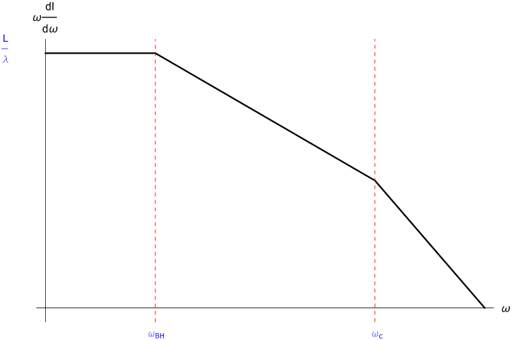
Figure 3.4: A log-log plot of the radiative energy loss spectrum across a range of different energies. As is described in the text, the BDMPS-Z and AMY formalisms capture the middle region, for which $\omega_{BH}\leq\omega\leq\omega_{c}$. The OE then correctly describes the BH region on the left, along with the single-scattering region on the right.

3.7 Recent Developments

Jet energy loss is still an extremely active topic of research, with there being a number of exciting advancements over the past decade or so. In particular, the Improved Opacity Expansion (IOE) is a powerful tool that has been developed [190, 195, 196, 197] to provide a unified description of the multiple, soft scattering and the single, hard scattering regimes for the case of a dense medium. Whereas the usual OE involves expanding in the number of elastic collisions, which is equivalent to expanding in powers of the dipole potential, $V(\mathbf{B})$ from Eq. (3.21), the IOE shifts the expansion point to HOA solution, i.e for $V(\mathbf{B})\sim\hat{q}_{0R}\mathbf{B}^{2}$. In doing so, the IOE resums multiple soft scatterings while also accounting for rare, harder scatterings. In fact, it has been highlighted recently [194] that for a dense medium, only the OE and IOE are needed to describe the entire medium induced spectrum. Their conclusion is solidified by comparison with the full, numerically constructed in-medium spectrum [198].

There has also been much progress with respect to the understanding of multiple in-medium splitting. It was only understood relatively recently that the colour coherence phenomenon that parton showers possess in the vacuum does not carry over to the case of a dense medium [199, 200, 201]. Instead, “anti-angular ordering” takes place, suppressing interference between successive gluon radiations. This has paved the way for the construction of an in-medium cascade [202, 203, 2, 204, 205, 206] that is differential in transverse momentum. The validity of these approaches is predicated on the fact that interference effects between gluons with overlapping formation times are not large. A series of papers by Arnold and collaborators [165, 207, 208, 209, 210, 211, 212, 213, 214, 215, 216, 217] have been devoted to exploring whether or not these latter interference effects are sizable. They claim, restricting the radiated gluons to have energies $\omega\gg T$ that most of the overlap effects can be absorbed into a redefinition of $\hat{q}_{R}(\mu_{\perp})$.

A large part of this thesis will be devoted to the discussion of double logarithmic corrections to $\hat{q}_{R}(\mu_{\perp})$ [218, 1, 2, 219, 18] at $\mathcal{O}(g^{2})$. These are radiative, quantum corrections that arise from keeping track of the recoil during the medium-induced emission of a gluon. Determining the precise region of phase space from which the double log originates is of paramount importance, as it of course controls whether they are large in comparison to $g^{2}$. While the calculations [1, 2] demonstrated the presence of these corrections, they did not strive to quantify them precisely, which, as we will see, turns out to be a difficult task. The double logarithmic corrections have been resummed [220, 221, 222, 223], effectively renormalising the leading order value of $\hat{q}_{R}(\mu_{\perp})$. It has also been shown that these double logs are universal [220, 224, 225]; they also appear in calculations with two emitted gluons with overlapping formation times in the final state, i.e in precisely the context of multiple emissions mentioned above.

Chapter 4 Tools for Studying Jets at Finite Temperature

Throughout the previous chapter, we have focused on motivating and discussing some of the basic ideas related to jet energy loss. Along the way, rigour is by and large sacrificed so as to make the physical picture more transparent. The theme of this thesis however is to provide and analyse corrections to two quantities, which in part control jet quenching, while maintaining a strong connection to first principles.

This connection is forged through the use of thermal field theory, which is to be introduced in Sec. 4.2. Before diving into this somewhat intricate topic, we choose to prepend some information regarding the general principles and features of effective field theory in Sec. 4.1. The rest of the chapter will then be focused on showing how two effective field theories: Electrostatic QCD and Hard Thermal Loop Effective Theory play a part in the higher order corrections to $\hat{q}$ and $m_{\infty}$ that we will ultimately be interested in computing.

4.1 Effective Field Theory and The Method of Regions

A common approach, practiced across many facets of physics is to take advantage of inherent scale separation, present in the relevant physical setup in order to drastically simplify calculations. Oftentimes, this is done almost unconsciously: one does not need to account for quantum gravity effects to accurately calculate planets’ orbits around the sun nor does one need worry about the bottom quark when calculating hydrogen’s energy levels, to give a couple of examples. For systems, whose dynamics are completely determined through their Lagrangian, the effective field theory (EFT) framework can provide a rigorous, yet extremely powerful tool through which, one can make otherwise daunting calculations more tractable, while at the same time rendering the physical picture more lucid. Below, we discuss some of the principles associated with the construction of EFTs, before briefly introducing a very helpful technique used for calculating loop integrals with multiple scales. We follow a combination of [226, 227, 228].

A Lagrangian density can generally be written as

$$\mathcal{L}=\sum_{i}C_{i}\mathcal{O}_{i}$$ (4.1)

where the $\mathcal{O}_{i}$ are operators and the $C_{i}$ are their respective couplings. For simplicity, we restrict ourselves to theories in $D=4$ spacetime dimensions. Since the action has to be dimensionless, a field’s dimension is always determined by its kinetic term. Thereafter, for each non-kinetic term, one can deduce the mass dimension of associated $C_{i}$ since the dimensions of all $\mathcal{O}_{i}$’s, being products of (possibly different) fields have already been fixed. We can then distinguish three classes of operators, sorted according to their dimension $d_{i}$. Operators with:

• $d_{i}<4$ are known as relevant.

• $d_{i}=4$ are known as marginal.

• $d_{i}>4$ are known as irrelevant.

A simple counting argument (see for instance Chapter $18$ of [22]) shows that an infinite number of counterterms are required to cancel the UV divergences (to all orders in perturbation theory) coming from irrelevant operators, thereby stripping the overarching theory of any predictive power. Thus, if Eq. (4.1) is to describe a renormalisable QFT in the traditional sense, the sum should only include marginal and relevant operators. In contrast, as we will now see, irrelevant operators turn out to be very important in effective field theories.

For simplicity, let us assume that we are interested in studying a QFT, describing two massive fields: $\phi_{1}$ with mass $m$ and $\phi_{2}$ with mass $M$. Moreover, we assume that the QFT is renormalisable in the traditional sense. We now want to write down an effective field theory (EFT), which only captures the dynamics below some scale, $\Lambda$ such that $M>\Lambda\gg m$. After implementing the cutoff, $\Lambda$ on the full theory’s generating functional one can in principle integrate out the heavy $\phi_{2}$ field from the path integral. Upon expanding the resultant Lagrangian powers of $1/M$, one recovers an infinite sum over local operators

$$\mathcal{L}_{\text{EFT}}=\mathcal{L}_{d_{i}\leq 4}+\sum_{i}\frac{c_{i}}{M^{d_{i}}}\mathcal{O}_{i},$$ (4.2)

where the $c_{i}$ above are dimensionless and are called Wilson coefficients. Note that the first term above contains the part of the original Lagrangian that only depends on $\phi_{1}$. The second term instead contains a sum over irrelevant operators $\mathcal{O}_{i}$, built from products (and possibly derivatives) of the $\phi_{1}$ field. But how does this mesh with our previous statement that irrelevant operators leave theories unrenormalisable? Observe that, around the small mass scale $m$ these operators should give a contribution to some measurable quantity that goes like $\sim c_{i}(m/M)^{d_{i}}$ with $d_{i}\geq 1$. It is then not difficult to see that one can truncate the sum in Eq. (4.2) according to the desired accuracy for the perturbative computation – here lies one of the great advantages of EFTs. Furthermore, even though the resultant EFT is not renormalisable in the traditional sense, it can be renormalised, order by order in the $(1/M)$ expansion, thereby maintaining its predictive capability.

The fact that terms with irrelevant operators in Eq. (4.2) are suppressed for
energies $\sim m\ll M$ is in some sense a formalising of the rather general comments made at the beginning of the section. It is nevertheless worth pointing out that the Wilson coefficients multiplying the irrelevant operators will inevitably contain information about the field that has been integrated out. To extract the dependence of the Wilson coefficients on the parameters of the higher-level theory, one generally has to perform what is known as a matching procedure.

In contrast to the notion of integrating out mentioned above, where one can actually do the functional integration, it is more often than not the case that even trying to perform such a manoeuvre is impractical. Instead, what one generally does is to construct the EFT theory by writing down a Lagrangian, which respects all of the symmetries that one wishes the low energy theory to respect, usually a subset of the symmetries associated with the higher-level theory. Then, once the Lagrangian has been truncated to the desired precision, matching conditions are imposed; by comparing diagrams from the two theories, $c_{i}^{\prime}s$ are chosen so that the EFT and higher-level theory agree in the regime where they are both valid. Matching is then performed order by order in the expansion parameter, which in the previous example was $(m/M)$.

While it is not so clear from the discussion above, computations in an EFT are usually considerably more simple due to the fact that one has reduced the number of scales in the problem. Even if there are multiple scales in the EFT, as long as these scales possess some scale separation, one can iterate the above procedure, producing a family of EFTs, each of which is well-suited to describe physics at a different scale. As an example, consider the reduction of QCD to non-relativistic QCD (NRQCD) [229], capable of describing heavy quarkonia. There, the hierarchy is $M\gg Mv$ where $M$ is the mass of the heavy quark, $v\ll 1$ is the relative velocity and $Mv$ is the typical momentum transfer. One can then integrate out the scale $Mv$, which is large compared to the binding energy $Mv^{2}$ and in doing so obtain potential NRQCD (pNRQCD) [230]. Another example of a so-called top-down EFT is soft collinear effective theory (SCET) [231, 232, 233, 234, 235], which capitalises on the separation between the so-called hard, collinear and soft scales in jet physics to efficiently resum Sudakov logarithms.

So far, we have restricted ourselves to EFTs where the underlying theory is known. There are also so-called bottom-up EFTs where the aforementioned method of matching is not applicable. Instead, one constrains the Wilson coefficients using experimental data or data from LQCD. This is the case for Chiral Perturbation Theory [236, 237], which allows one to study the low-energy dynamics based on the underlying chiral symmetry. Indeed, a more modern take on QFT is that every theory is an EFT! The practice of adding irrelevant operators to the Standard Model Lagrangian goes under the name Standard Model Effective Theory or SMEFT [238, 239].

Before moving on, by giving a simple example, we wish to elucidate the usefulness of a strategy that will be used throughout this thesis, known as the method of regions [240, 241]. To start, consider the following integral, where for the sake of simplicity we work in $2$ spatial dimensions

$$I=\int\frac{d^{2}P}{(2\pi)^{2}}\frac{1}{(P^{2}+m^{2})(P^{2}+M^{2})}.$$ (4.3)

The integration is evidently finite so no regularisation is necessary. After Feynman parameterisation, we immediately get

$$I=\frac{1}{4\pi(m^{2}-M^{2})}\ln\frac{m^{2}}{M^{2}}.$$ (4.4)

Now let us consider the limit where there is a scale separation, i.e $m\ll M$ so that we can expand for large $M$

$$I=\frac{1}{4\pi M^{2}}\ln\frac{m^{2}}{M^{2}}\Big{(}1+\frac{m^{2}}{M^{2}}+\mathcal{O}(m^{4})\Big{)}.$$ (4.5)

So far, all we have done is calculated a simple integral. But let us now go back Eq. (4.3) and see what happens if we perform the expansion before doing the integration. First, we consider the region where $P\sim m\ll M$. There,

$$I_{P\sim m} =\int\frac{d^{2}P}{(2\pi)^{2}}\frac{1}{(P^{2}+m^{2})M^{2}}\left(1-\frac{P^{2}}{M^{2}}+\mathcal{O}(P^{4})\right)$$

$$=\frac{1}{4\pi M^{2}}\left(\ln\frac{\Lambda^{2}}{m^{2}}+\frac{m^{2}}{\Lambda^{2}}-\frac{\Lambda^{2}}{M^{2}}+\frac{m^{2}}{M^{2}}\ln\frac{\Lambda^{2}}{m^{2}}+\mathcal{O}(m^{4})\right),$$ (4.6)

where we have cut off the integration in the UV with $\Lambda\gg m$. Next, let us consider the region $P\sim M\gg m$. Here, $\Lambda\ll M$ instead acts as an IR cutoff

$$I_{P\sim M} =\int\frac{d^{2}P}{(2\pi)^{2}}\frac{1}{(P^{2}+M^{2})p^{2}}\left(1-\frac{m^{2}}{p^{2}}+\mathcal{O}(\frac{1}{P^{4}})\right)$$

$$=\frac{1}{4\pi M^{2}}\left(\ln\frac{M^{2}}{\Lambda^{2}}+\frac{\Lambda^{2}}{M^{2}}-\frac{m^{2}}{\Lambda^{2}}+\frac{m^{2}}{M^{2}}\ln\frac{M^{2}}{\Lambda^{2}}+\mathcal{O}(m^{4})\right).$$ (4.7)

If we add the contributions from the two regions together, we recover the full result Eq. (4.5). While this expected, note that for the combined result to be $\Lambda$ independent, all of the corrections depending on a power of $\Lambda$ must cancel. This turns out to be a general result: given some loop integral with multiple scales (in our case, $m$ and $M$), we can make use of the strategy:

• By power counting, identify the different regions that will give a finite contribution to the integral. In the example above, these regions were $P\sim m$ and $P\sim M$.

• Expand appropriately in those regions and then perform the integration. While the integral above was simple enough to calculate without resorting to this method, if there are more scales, or the integrand is more complicated, this can be a formidable task.

• Add the contributions from the different regions together. Corrections depending on a power law of the introduced cutoff will cancel, leaving only logarithms of ratios of the separated scales and/or finite terms. Most of the time, we throw away the power law corrections prior to this step, since we know they will cancel out anyway. But in some cases, one can take advantage of this feature of power law corrections: if it is not a priori clear which regions contribute to the full integral, one can use power law correction cancellation as a proxy for checking whether two regions are adjacent. This is essentially what is done in Sec. 5.8.

Such a protocol is followed for many of the calculations performed in this thesis.

Despite our example above being extremely simple, it easy to see how this strategy conveniently compliments the EFT philosophy. If some quantity of interest is given in terms of an integral, $I$, one can do a power counting, thereby identifying the different regions, over which integrating will contribute to $I$. For certain regions, the contribution may then be much easier to compute using some EFT. Consider $\hat{q}(\mu_{\perp})$, which receives a contribution from the region $P\sim T$ and also from the region $P\sim gT$ at LO in the strong coupling. The contribution from the former region is computed using finite temperature QCD, whereas the latter is computed either with Hard Thermal Loop effective theory or electrostatic QCD, both of which will be introduced in the next sections. The LO soft contribution is computed in Sec. 4.4.1. For $m_{\infty}$, the LO value only receives a hard contribution, whereas the NLO correction only receives a soft contribution. The computation of the NLO correction is contained in Sec. 4.4.2.

Before moving on, we make a remark with respect to the choice of regulator used above. In that example, we regulated the integration in each region with a hard cutoff in order to explicitly show the cancellation of the terms depending on power laws of $\Lambda$. Nevertheless, whenever possible, we will choose to instead use dimensional regularisation (DR). This is well-justified as:

• Unlike cutting off with a hard regulator, DR preserves Lorentz and gauge invariance.

• Scaleless integrals vanish. In thermal field theory calculations, where one has to do a vacuum subtraction, this is an especially convenient choice since the vacuum terms are usually scaleless.

• Logarithmic divergences show up as $1/\epsilon$ poles. Conversely, power law divergences do not appear at all.

See App. A for our conventions for DR.

4.2 Thermal Field Theory

The generalisation of perturbative quantum field theory to finite temperatures traditionally goes under the name of thermal field theory (TFT). This section will therefore be devoted to explaining how concepts from quantum statistical mechanics can be consistently implemented in a QFT context. In doing, so we will arrive at two different, but equivalent formulations of TFT: the Imaginary Time Formalism (ITF) and the Real Time Formalism (RTF). Essentially all of the calculations in Ch. 5 and Ch. 6 will be done in the RTF. Much of Sec. 4.2.3 will therefore be spent on introducing the propagators to be used in later chapters. We will nevertheless also make a point to explore the ITF, as it allows for a cleaner derivation of the effective theory, Electrostatic QCD, which plays a central role in the calculations that we are trying to build upon in this thesis. Throughout this section, we only work towards sketching a derivation of the finite temperature propagators for bosons. The fermion propagators will instead be stated, with the occasional remark made when necessary. Moreover, we set all chemical potentials to zero throughout, as the phenomena that we investigate in this thesis only take place near the $\mu=0$ axis of the QCD phase diagram. We follow a combination of [242, 175, 166].

4.2.1 The Imaginary Time Formalism

An important difference between zero and finite temperature QFT is that in the latter case, it is necessary to take into account statistical fluctuations (in addition to quantum fluctuations), which arise from only having limited, macroscopic information of the entire system at some moment $t_{0}$. The density operator

$$\rho(t_{0})=\sum_{i}p_{i}(t_{0})\ket{i}\bra{i},$$ (4.8)

is an important object in this context. In particular, the $p_{i}(t_{0})$ represent the probabilities associated with the different pure states, whose linear combination define the mixed state, described by $\rho(t_{0})$. In equilibrium, it takes the form

$$\rho_{\text{eq}}=\frac{1}{Z}e^{-\frac{H}{T}}$$ (4.9)

where

$$Z=\Tr e^{-\frac{H}{T}}$$ (4.10)

is the partition function and $H$ is the Hamiltonian operator describing a field theory for a scalar field, $\varphi(X)$. The route to the derivation of the ITF starts by identifying $\tau=-i/T$ above and then recognising that the operator in the trace is a time evolution operator in imaginary time, $e^{-iH\tau}$. One then proceeds to use the standard techniques introduced by Feynman, evaluating the trace using the eigenstates of the field operator, $\varphi(X)$. Following [243], one can write $Z$ as a Euclidean path integral

$$Z(\beta)=\int\mathcal{D}\varphi\exp\Big(-S_{\text{E}}(\beta)\Big{missing})$$ (4.11)

where

$$S_{\text{E}}(\beta)=\int_{0}^{\beta}d\tau\int d^{3}x\mathcal{L}(\varphi),$$ (4.12)

and $\beta\equiv 1/T$. The cyclicity property of the trace in Eq. (4.10) is moreover implemented by the condition that $\varphi(0,\vec{\mathbf{x}})=\pm\varphi(0,\vec{\mathbf{x}})$, where $+$ ($-$) is the correct choice for bosons (fermions).

Of course, we would like to be able to compute thermal expectation values of composite operators

$$\langle\mathcal{O}\rangle=\frac{\int\mathcal{D}\varphi\exp\Big(-S_{\text{E}}(\beta)\Big{missing})\mathcal{O}}{Z(\beta)}.$$ (4.13)

Such a goal motivates the inclusion of a source term to the partition function

$$Z(\beta)=\int\mathcal{D}\varphi\exp\Big(-S_{\text{E}}(\beta)+\int_{0}^{\beta}d^{4}Xj(X)\varphi(X)\Big{missing}).$$ (4.14)

so that the thermal expectation values can be obtained from the usual methods of functional differentiation.

After appropriately shifting the field $\varphi(X)$, one recovers

$$Z_{F}(\beta,\,j)=\int \mathcal{D}\varphi$$ ,

at which stage the Gaussian functional integration over $\varphi(X)$ can be performed, resulting in

$$Z_{F}(\beta,\,j)=Z_{F}(\beta,\,0)\exp\Big(\frac{1}{2}\int_{0}^{\beta}d^{4}Xd^{4}Yj(X)\Delta_{F}(X-Y)j(Y)\Big{missing}).$$ (4.15)

As can be readily verified using Eq. (4.13) and functional differentiation methods (see [242] for details), $\Delta_{F}(X-Y)$ is the time-ordered (in imaginary time) two-point function,

$$\Delta_{F}(\tau,\vec{\mathbf{x}})=\langle\mathcal{T}\varphi(\tau,\vec{\mathbf{x}})\varphi(0,\vec{\mathbf{0}})\rangle.$$ (4.16)

$\mathcal{T}$ denotes time-ordering in imaginary time and the cyclicity of the trace in Eq. (4.10) fixes $\tau$ to lie in the interval $[0,\beta]$ with periodicity $\tau\to\tau-\beta$. Progressing onward, let us note that $\delta(\tau,\vec{\mathbf{x}})$ solves the partial differential equation

$$\Big{(}-\frac{\partial^{2}}{\partial\tau^{2}}-\nabla^{2}+m^{2}\Big{)}\Delta_{F}(X-Y)=\delta(\tau_{X}-\tau_{Y})\delta(\vec{\mathbf{x}}-\vec{\mathbf{y}}).$$ (4.17)

It is then possible to find a solution by Fourier transforming to momentum space

$$\Delta(\omega_{n},\vec{\mathbf{k}})=\frac{1}{\omega_{n}^{2}+k^{2}+m^{2}},$$ (4.18)

which leaves us with the Euclidean or Matsubara propagator [244]. The periodicity of imaginary time is reflected above through the fact that the so-called Matusbara frequencies are forced to take on discrete values, $\omega_{n}=2\pi nT\,,\,n\in\mathbb{Z}$.

With the free propagator in hand, one can then deform the theory by adding a potential term and proceed to work out the Feynman rules, similarly to the $T=0$ case. The main difference here is however, that in loop computations, instead of integration over continuous frequencies, one is left having to perform an infinite sum over the discrete Matsubara frequencies. When computing time-dependent quantities in the ITF, the infinite sum must be evaluated before analytically continuing back to real time. For this reason, the ITF’s main domain of applicability is largely restricted to the computation of thermodynamic quantities.

Before progressing to the case of QCD, we mention that analytical continuation to arbitrary (non-discrete) frequency values is provided by

$$\Delta(z,\vec{\mathbf{k}})=\int_{-\infty}^{\infty}\frac{dk^{0}}{2\pi}\frac{\rho_{\text{B}}(k_{0},\vec{\mathbf{k}})}{k^{0}-z}$$ (4.19)

with $\rho_{\text{B}}(k_{0},\vec{\mathbf{k}})$ the spectral function for bosons. Indeed, choosing $z=k^{0}\pm i\varepsilon$ with real $k^{0}$ allows us to recover the causal propagators. Specifically,

$$D_{R}(k^{0},\vec{\mathbf{k}})=-i\Delta(z=k^{0}+i\varepsilon)\quad,\quad D_{A}(k^{0},\vec{\mathbf{k}})=-i\Delta(z=k^{0}-i\varepsilon).$$ (4.20)

The retarded propagator, $D_{R}$ is thus analytic in the upper half complex $k^{0}$ plane whereas the advanced propagator, $D_{A}$ is analytic in the lower half complex $k^{0}$ plane. The above relations will be used in Sec. 4.3.

As in the $T=0$ case, much of what has been discussed above can be adapted without too much difficulty to the case of a gauge theory, such as QCD. We point out that fermions in the partition function Eq. (4.11) should have anti-periodic boundary conditions in contrast to their bosonic counterparts. It then transpires that the Matsubara frequencies for the quarks are instead $\omega_{n}=(2n+1)\pi T,\,n\in\mathbb{Z}$. Another issue that is familiar from zero temperature QFT is that of the integration over unphysical gauge field configurations in the path integral. One can nevertheless bypass this issue through the inclusion of ghosts, through a suitably generalised Fadeev-Popov procedure. Since the details pertaining to such a procedure will not be relevant for what is to follow, we refer the reader to the textbooks [245, 242] for more information. Renormalisation, which is of course also relevant for the scalar field case, need not be worried about at finite temperature. This stems from the fact that the new scale, $T$ does not modify the theory at short distances $\ll 1/T$, and thus it is safe to assume that UV divergences will carry over from the $T=0$ theory. When computing thermal contributions to quantities of interest in the ITF or RTF, one usually subtracts off the vacuum result anyway, which is thus equivalent to renormalisation. On the other hand, the scale $T$ significantly disturbs the IR structure of the theory (again, this is also true for the scalar field). We take this opportunity to write down the QCD Lagrangian (with massless quarks) in Euclidean space

$$\mathcal{L}^{\text{QCD}}_{\text{E}}=\frac{1}{4}F_{\mu\nu}F^{\mu\nu}+\bar{\psi}_{i}\not{D}\psi_{i},$$ (4.21)

where the sum is over the quark flavours.

4.2.2 Dimensional Reduction

At zero temperature, we can roughly say that perturbation theory is done in $g^{2}$, owing to the fact that loops are added at a cost of $g^{2}/4\pi$ (see Eq. (2.14)). As we will now sketch, things become much more complicated when $T>0$ because of the inclusion of additional scales. To show in a more concrete way how these complications arise, let us consider, as an example, the contribution to the pressure from the gluonic sector. It takes the following schematic form

$$P^{G}\sim\int d^{3}p\,p\,n_{\text{B}}(E_{p})$$ (4.22)

where $E_{p}$ is the energy and

$$n_{\text{B}}(E_{p})\equiv\frac{1}{e^{\frac{E_{p}}{T}}-1}$$ (4.23)

is the Bose-Einstein distribution function. $T$ is often denoted the hard scale: it represents the average energy of quarks and gluons in the plasma and is also the scale associated with the Matsubara frequencies. From Eq. (4.22), its contribution to the pressure can be estimated as

$$P^{G}_{\text{hard}}\sim T^{4}n_{\text{B}}(T)\sim T^{4}+\mathcal{O}(g^{2}).$$ (4.24)

As long as $g^{2}\ll 1$, the perturbative expansion is still evidently well-defined for contributions coming from this scale. There is also the soft scale $gT$, which, as we will see in Sec. 4.2.4 is the momentum associated with collective excitations in the plasma. Its contribution reads

$$P^{G}_{\text{soft}}\sim(gT)^{4}n_{\text{B}}(gT)\sim g^{3}T^{4}+\mathcal{O}(g),$$ (4.25)

where the perturbative expansion still converges, albeit in a slower manner, due to the fact that $n_{\text{B}}(E_{p})\sim T/E_{p}$ if $E_{p}\ll T$. The diverging of the statistical function in this regime is known as Bose enhancement. Finally, the ultrasoft scale $\sim g^{2}T$ gives

$$P^{G}_{\text{ultra soft}}\sim(g^{2}T)^{4}n_{\text{B}}(g^{2}T)\sim g^{6}T^{4}+\mathcal{O}(1).$$ (4.26)

In other words, higher loop corrections to the contribution from the ultrasoft scale come at no cost! For this reason, the ultrasoft scale is sometimes called the non-perturbative scale. In this case, the contribution from the ultrasoft scale only enters at $\mathcal{O}(g^{6})$, which turns out to be at four-loop order. Yet, there are other quantities of interest, such as the transverse scattering rate $\mathcal{C}(k_{\perp})$, discussed in Sec. 3.4, that already receive these kinds of non-perturbative contributions at leading order. Such a seemingly ubiquitous feature was identified by Linde in the 1980’s [246] and at first glance, seems to cast much doubt on the validity of perturbation theory at finite temperature. Note that this issue is unique to the gauge sector of QCD; the fermionic analogue of Eq. (4.22) would instead possess a factor of

$$n_{\text{F}}(E_{p})\equiv\frac{1}{e^{\frac{E_{p}}{T}}+1},$$ (4.27)

the Fermi-Dirac distribution function, which instead has the property that $n_{F}(E_{p})\sim 1/2$ for $E_{p}\ll T$.

Fortunately, much progress has been made in circumventing these issues related to the gauge sector’s behaviour in the IR. Two approaches have proven successful in this pursuit: dimensional reduction and Hard Thermal Loop effective theory. The latter EFT will be introduced subsequent to the discussion about the RTF.

In the mid-1990s, Braaten and Nieto popularised the use of Electrostatic QCD (EQCD), an effective field theory derived by integrating out the hard scale, $\pi T$ or said differently, all but the zero Matsubara mode from finite temperature QCD [247, 248]. Since there is only one Matsubara mode left, the Euclidean time direction is effectively eliminated – this is where the term dimensional reduction [249, 250] comes from. EQCD is thus also said to be a theory of static modes. A novel consequence of this reduction is that the $A^{0}$ field, no longer possessing a gauge symmetry is allowed to acquire a mass, $m_{D}\sim gT$, known as the Debye mass. This component, which we denote as $\Phi=iA_{0}$, now transforms as a scalar in the adjoint representation of SU(N). EQCD’s Lagrangian can be derived, following the procedure roughly described in the previous section

$$\mathcal{L}_{\text{EQCD}}=\frac{1}{2}\Tr F_{ij}F_{ij}+\Tr D_{i}\Phi D_{i}\Phi+m_{D}^{2}\Tr\Phi^{2}+\lambda_{E}\left(\Tr\Phi^{2}\right)^{2}.$$ (4.28)

The fields $A_{i}=A_{i}^{a}T^{a}$ now live in three dimensions and $D_{i}=\partial_{i}-ig_{3\text{d}}A_{i}$, where $g_{3\text{d}}^{2}=g^{2}T$ at LO. The $\lambda_{E}$ term is a remnant of the four-$A^{0}$-interaction that arises in two-loop level in full-QCD perturbation theory.

This procedure can be iterated, integrating out the field, $\Phi$ or equivalently the soft scale, $gT$. We are then left with three-dimensional pure Yang-Mills theory, coined Magnetostatic QCD or MQCD, which only depends on the ultrasoft scale $g^{2}T$. At present day, perturbative matching onto these dimensionally reduced theories is a mature, well-understood technology, with the EFT couplings having been computed up to $\mathcal{O}(g^{6})$ [251, 250, 252]. Moreover, it turns out [248] that the contribution to the pressure can be written as

$$P^{G}=P^{G}_{\text{hard}}+P^{G}_{\text{EQCD}}+P^{G}_{\text{MQCD}}.$$ (4.29)

In other words, one can compute in the three different theories to obtain a result for the pressure up to $\mathcal{O}(g^{6})$, which is free of IR divergences. Such an achievement marks a true tour de force of the dimensional reduction framework. The hard contribution was computed in [253] with the soft contribution obtained perturbatively in [254, 255] and the MQCD contribution in [256, 257] on the lattice. Indeed, a detail that we have glossed over up until this point is that these dimensionally reduced theories can be studied non-perturbatively with the use of three-dimensional lattice simulations; with the disappearance of the time direction, one does not need to worry about complications arising from analytically continuing back to real time. Nevertheless, as these EFTs are naturally derived within the ITF, their applicability has been historically restricted to the computation of thermodynamic quantities. This is what makes their recent deployment to the study of real-time, dynamical quantities all the more impressive [11], to be discussed in Sec. 4.3.

4.2.3 The Real Time Formalism

From the previous section alone, it is easy to see why one would like to have a formalism of thermal field theory in which time is kept real from the outset. One can start on this path by analytically continuing the Euclidean propagator Eq. (4.18) to real time [258]. This yields, for a scalar field

$$D_{F}(K)=\frac{i}{K^{2}-m^{2}+i\varepsilon}+2\pi\delta(K^{2}-m^{2})n_{\text{B}}(|k^{0}|).$$ (4.30)

Despite the appealing feature of this expression, specifically, that there is a clear separation of the vacuum and thermal parts, doing perturbation theory with this propagator alone results in so-called pinch singularities, where products of identical delta functions appear in loop integrals.

Figure 4.1: Illustration of the Schwinger-Keldysh contour in the complex t-plane. Image taken from [166].

The starting point of the RTF instead consists of going back to Eq. (4.11) and deforming the contour in the following way: as is depicted in Fig. 4.1, one begins from (real) $t_{0}$ and integrates along the real axis to $t_{1}$. The contour is then deformed below the real axis by an amount $-i\varepsilon$ before being brought back across the imaginary axis to $t_{0}-i\varepsilon$. Finally, the path follows a vertical straight line from $t_{0}-i\varepsilon$ to $t_{0}-i\beta$. The choice of path is known as the Schwinger-Keldysh contour, named after its authors [259, 260]. It turns out that in taking $t_{0}\to-\infty$ and $t_{1}\to+\infty$, contributions coming from integrating over the vertical portions of the contour factorise, appearing as overall multiplicative constants [261, 262] and, per Eq. (4.13) are not relevant for the computation of correlation functions. Note that this in contrast to the ITF, where the time $t_{0}$ is arbitrary. This can be seen by observing that the equilibrium density operator in Eq. (4.9) commutes with the Hamiltonian, implying that the equilibrium state is time translation invariant.

The price to pay for insisting on a framework where time is kept real is the so-called doubling of degrees of freedom, which becomes apparent when we write the generating functional

$$Z[j_{1},j_{2}]=\int\mathcal{D}\varphi_{1}\mathcal{D}\varphi_{2}e^{iS[\varphi_{1}]-iS[\varphi_{2}]-\int d^{4}X\Big{(}j_{1}(X)\varphi_{1}(X)-j_{2}(X)\varphi_{2}(X)\Big{)}},$$ (4.31)

with

$$j_{1}(X)=j(t,\vec{\mathbf{x}})\quad\quad j_{2}(X)=j(t-i\varepsilon,\vec{\mathbf{x}})$$ (4.32)

and functional differentiation defined by

$$\frac{\delta j_{a}(X)}{\delta j_{b}(X^{\prime})}=\delta_{ab}\delta^{4}(X-X^{\prime}).$$ (4.33)

The “1” fields can be thought of living on the upper horizontal branch in Fig. 4.1 and are associated with physical particles. Conversely, the “2” fields live on the lower branch and act like ghosts in the sense that the are only to be included as internal lines when calculating time-ordered amplitudes. The vertices from type 2 fields come with an extra minus sign because of the different signs of the actions in Eq. (4.31). As a result of the doubling of degrees of freedom, the scalar theory’s propagator appears as a matrix in 1,2 space [242]

$$\mathbf{D}_{ij} =\frac{\delta}{\delta j_{i}}\frac{\delta}{\delta j_{j}}Z[j_{1},j_{2}]\bigg{|}_{j_{1}=0,\,j_{2}=0}$$

$$\mathbf{D} =\left(\begin{array}[]{cc}\langle\varphi_{1}\varphi_{1}\rangle&\langle\varphi_{1}\varphi_{2}\rangle\\ \langle\varphi_{2}\varphi_{1}\rangle&\langle\varphi_{2}\varphi_{2}\rangle\end{array}\right)=\left(\begin{array}[]{ccc}D_{F}&&D_{>}\\ D_{<}&&D_{\bar{F}}\end{array}\right).$$ (4.38)

The $11$ and $22$ entries are the time-ordered and anti-time-ordered propagators

$$D_{F}(t_{1},t_{0}) =\Theta(t_{1}-t_{0})\langle\varphi(t_{1})\varphi(t_{0})\rangle+\Theta(t_{0}-t_{1})\langle\varphi(t_{0})\varphi(t_{1})\rangle$$ (4.39)

$$D_{\bar{F}}(t_{1},t_{0}) =\Theta(t_{0}-t_{1})\langle\varphi(t_{1})\varphi(t_{0})\rangle+\Theta(t_{1}-t_{0})\langle\varphi(t_{0})\varphi(t_{1})\rangle$$ (4.40)

respectively, where we choose to suppress the spatial argument for the moment. The off-diagonal entries are the cut or Wightman propagators, which describe physical correlations in the medium. They can be written in terms of the spectral function,

$$\rho_{\text{B}}(t_{1},t_{0})=\langle[\varphi(t),\varphi(0)]\rangle=D_{>}(t_{1},t_{0})-D_{<}(t_{1},t_{0}).$$ (4.41)

We also find it useful to define the retarded and advanced propagators in terms of the spectral function

$$D_{R}(t_{1},t_{0}) =\Theta(t_{1}-t_{0})\rho_{\text{B}}(t_{1},t_{0})$$ (4.42)

$$D_{A}(t_{1},t_{0}) =-\Theta(t_{0}-t_{1})\rho_{\text{B}}(t_{1},t_{0})$$ (4.43)

so that we can write

$$\rho_{\text{B}}(t_{1},t_{0})=D_{R}(t_{1},t_{0})-D_{A}(t_{1},t_{0}).$$ (4.44)

Note that the propagators $D_{R}(t_{1},t_{0}),\,D_{A}(t_{1},t_{0})$ are known as causal propagators.

Figure 4.2: Vertices appearing in the RTF for a scalar field with a quartic interaction in the 1,2 basis. Vertices connecting propagators associated with the 2 fields come with a relative change of sign because of the extra minus in Eq. (4.31). Image taken from [166].

Many of these objects are integral to TFT calculations, in contrast to the situation at zero temperature, where in order to do perturbation theory, all one really needs is the time-ordered propagator. This is because, at zero temperature, one is able to utilise Lehmann-Symanzik-Zimmermann (LSZ) reduction in order to relate vacuum expectation values of time-ordered operators to S-matrix elements and hence, experimentally accessible quantities such as particle cross-sections. Such a manoeuvre is predicated on the assumption that the particles taking part in such a process correspond to asymptotic states, created infinitely far away in the past or future. Yet at finite temperature, random interactions induced by the medium do not preserve any state, implying that S-matrix elements do not play such a central role.

For a generic density operator, only three of the five correlators are independent. However, in equilibrium, the Kubo-Martin-Schwinger (KMS) relation [263, 264] provides another constraint

$$D_{>}(t)=D_{<}(t+i\beta),$$ (4.45)

which in momentum space reads

$$D_{>}(k^{0})=\int dte^{ik^{0}t}D_{>}(t)=e^{\beta k^{0}}D_{<}(k^{0}).$$ (4.46)

Moreover, the cut propagators can be expressed in terms of the spectral function

$$D_{>}(K) =\left(1+n_{\text{B}}\left(k^{0}\right)\right)\rho_{\text{B}}(K)$$ (4.47)

$$D_{<}(K) =n_{\text{B}}\left(k^{0}\right)\rho_{\text{B}}(K)$$ (4.48)

where we have reinstated the full momentum dependence, as the above relations will be used repeatedly throughout this thesis. Notice that for the case of fermions, there is a sign difference, i.e

$$S_{>}(K) =\left(1-n_{\text{F}}\left(k^{0}\right)\right)\rho_{\text{F}}(K)$$ (4.49)

$$S_{<}(K) =-n_{\text{F}}\left(k^{0}\right)\rho_{\text{F}}(K)$$ (4.50)

The spectral functions are related to the causal propagators by

$$\rho_{\text{B}}(K) =D_{R}(K)-D_{A}(K)$$ (4.51)

$$\rho_{\text{F}}(K) =S_{R}(K)-S_{A}(K)$$ (4.52)

and finally, we can write the momentum space analogues of Eqs. (4.39),  (4.40) as

$$D_{F}(K)=\frac{1}{2}\Big{[}D_{R}(K)+D_{A}(K)\Big{]}+\left(\frac{1}{2}+n_{\text{B}}\left(k^{0}\right)\right)\rho_{\text{B}}(K)$$ (4.53)

$$D_{\bar{F}}(K)=-\frac{1}{2}\Big{[}D_{R}(K)+D_{A}(K)\Big{]}+\left(\frac{1}{2}+n_{\text{B}}\left(k^{0}\right)\right)\rho_{\text{B}}(K).$$ (4.54)

We also take this opportunity to define the symmetric rr-propagator

$$D_{rr}(K)\equiv\frac{1}{2}(D_{>}(K)+D_{<}(K))=\left(\frac{1}{2}+n_{\text{B}}\left(k^{0}\right)\right)\rho_{\text{B}}(K),$$ (4.55)

whose label will now be elaborated on.

While the “1,2” basis that we have used so far is easy to understand in terms of the Schwinger-Keldysh contour from Fig. 4.1, it is not unique. We write down here the propagators associated with the so-called “r/a” basis [260, 265], which is more convenient to work with for certain calculations. We start by defining

$$\varphi_{r}\equiv\frac{1}{2}\left(\varphi_{1}+\varphi_{2}\right),\quad\quad\varphi_{a}\equiv\varphi_{1}-\varphi_{2},$$ (4.56)

which produces a propagator matrix

$$\mathbf{D}=\left(\begin{array}[]{cc}\langle\varphi_{r}\varphi_{r}\rangle&\langle\varphi_{r}\varphi_{a}\rangle\\ \langle\varphi_{a}\varphi_{r}\rangle&\langle\varphi_{a}\varphi_{a}\rangle\end{array}\right)=\left(\begin{array}[]{ccc}D_{rr}&&D_{R}\\ D_{A}&&0\end{array}\right).$$ (4.57)

The vanishing of the aa propagator to all orders in perturbation theory can be seen by plugging the definitions Eqs. (4.39),  (4.40) into $\langle\varphi_{a}\varphi_{a}\rangle$ and using that
$\Theta(t_{1}-t_{0})+\Theta(t_{0}-t_{1})=1$.

We take a moment to clarify our conventions in the r/a formalism, as some of its features can appear quite confusing at first glance. As opposed to the 1,2 basis, where vertices are restricted to connect fields of the same type, there is mixing in the r/a formalism. To elaborate on what is meant by this, consider the quartic interaction, translated to the r/a basis, i.e

$$\frac{1}{4!}\left(\varphi_{1}^{4}-\varphi_{2}^{4}\right)=\frac{1}{2^{2}}\frac{1}{3!}\varphi_{a}^{3}\varphi_{r}+\frac{1}{3!}\varphi_{r}^{3}\varphi_{a}.$$ (4.58)

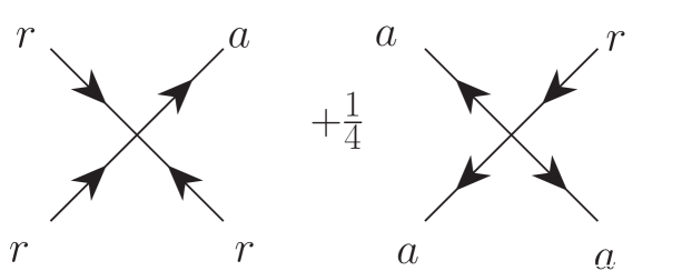
Figure 4.3: Vertices appearing in the RTF for a scalar field with a quartic interaction in the r/a basis. Image taken from [166].

It is not difficult to check that this structure will persist even in QCD; there are only vertices with an odd number of a fields, thus leaving us with only rra and aaa assignments. For vertices with more than one a-field, there is an extra factor of $1/2$ for each extra a line. This extra prefactor is indicated in Fig. 4.3.

We emphasise that the labels in Fig. 4.3 refer to the nature of the field at the vertex itself. In other words, each of the propagators with an r label in Fig. 4.3 could be either $\langle\varphi_{r}\varphi_{r}\rangle$ or $\langle\varphi_{r}\varphi_{a}\rangle$. We further stress that the arrows in Fig. 4.3 refer to the direction of causality (as opposed to the direction of momentum). The causal arrow associated with retarded (advanced) propagators always goes in the same (opposite) direction as the momentum flow. For rr propagators, causality instead flows in both directions, outward towards the vertices that the propagator is attached to.

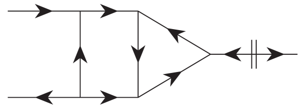
Figure 4.4: Example of a diagram that vanishes due to causality. The line on the far-right with a cut going through it is an rr propagator. Image taken from [166].

Despite the appearance of additional baggage, it is this transparency of causality flow that renders the r/a basis useful. In particular, closed loops of causality, which cause diagrams to vanish are visibly manifest in this formalism. A closed loop of causality is present when vertices at $t_{0}$, $t_{1}$, are connected by a product of (both) retarded and advanced propagators as is shown in Fig. 4.4. Their vanishing can then be explicitly seen by noting that the step functions in Eqs. (4.42),  (4.43) cannot be simultaneously satisfied.

Before concluding this section, for future reference, we write down both the free causal and rr gluon propagators in Coulomb gauge [166]. As was already mentioned, we forego commenting on the details related to gauge fixing at finite temperature

$$G^{00}_{R/A}(K) =\frac{i}{k^{2}},\quad\quad G^{ij}_{R/A}(K)=\frac{i(\delta^{ij}-\hat{k}^{i}\hat{k}^{j})}{K^{2}\pm i\varepsilon k^{0}}$$ (4.59)

$$G^{00}_{rr}(K) =0,\quad\quad G^{ij}_{rr}(K)=(\delta^{ij}-\hat{k}^{i}\hat{k}^{j})\left(\frac{1}{2}+n_{\text{B}}\left(|k^{0}|\right)\right)2\pi\delta(K^{2})$$ (4.60)

and Feynman gauge

$$G^{\mu\nu}_{R/A}(K) =-\frac{i\eta^{\mu\nu}}{K^{2}\pm i\varepsilon k^{0}}=\eta^{\mu\nu}G_{R/A}(K)$$ (4.61)

$$G^{\mu\nu}_{rr}(K) =-\eta^{\mu\nu}\left(\frac{1}{2}+n_{\text{B}}\left(k^{0}\right)\right)2\pi\varepsilon(k^{0})\delta(K^{2})=\eta^{\mu\nu}G_{rr}(K),$$ (4.62)

where we note that the appearance of the delta function in the rr propagators is due to the presence of the free spectral function

$$\rho_{\text{B}}(K)=2\pi\varepsilon(k^{0})\delta(K^{2}).$$ (4.63)

For completeness, we also list the free causal and rr propagators for fermions

$$S_{R/A}(K) =\frac{i\not{K}}{K^{2}\pm i\varepsilon k^{0}}$$ (4.64)

$$S_{rr}(K) =\not{K}\left(\frac{1}{2}-n_{\text{F}}\left(k^{0}\right)\right)2\pi\varepsilon(k^{0})\delta(K^{2}),$$ (4.65)

where

$$\rho_{\text{F}}(K)=2\pi\varepsilon(k^{0})\not{K}\delta(K^{2}).$$ (4.66)

is the free fermionic spectral function. These expressions, along with the vertices specified in App. A and the Hard Thermal Loop propagators to be given in the next section, supply the toolkit, which we draw from to perform real-time, perturbative calculations throughout the rest of the thesis.

4.2.4 Hard Thermal Loops

In Sec. 4.2.1, we highlighted the Linde problem [246] and mentioned that it can be in some sense bypassed through the use of dimensional reduction, which provides a route towards the computation of IR finite thermodynamic quantities. Another method, which rather cures a naive modelling of the interaction between hard and soft modes is supplied by Hard Thermal Loop (HTL) Effective Theory, first derived in the ITF by Braaten and Pisarski [266, 267], Frenkel and Taylor [268, 269] and Taylor and Wong [270]. We choose to introduce the HTL in the RTF [271] so that the formulas presented here can be directly applied to the calculations that will follow in later sections.

HTLs are regions of phase space in loop diagrams where the internal (loop) momentum is hard, i.e $\sim T$ and the momenta of the external legs is soft, i.e $\ll T$. It turns out that these loops can be added at no parametric cost and thus need to be resummed. To understand why, consider the retarded vacuum polarisation diagram with a hard thermal loop but soft external gluon legs. Using the Feynman rules from the previous section, taking $P\gg K$, where $P$ is the loop momentum and $K$ the external momentum [242]

$$\Pi^{\mu\nu}_{R}(K)=-m_{D}^{2}\int\frac{d\Omega_{v}}{4\pi}\bigg{(}\delta^{\mu}_{0}\delta^{\nu}_{0}+v^{\mu}v^{\nu}\frac{k^{0}}{v\cdot K+i\varepsilon}\bigg{)},$$ (4.67)

where $m_{D}^{2}=g^{2}T^{2}(N_{c}+T_{F}N_{F})/3$ is the leading order Debye mass, $v\equiv P/p^{0}=(1,\vec{\mathbf{p}}/p^{0})$ and we are working in the Coulomb gauge. The key point is that, for $K\sim gT$, the denominator of the retarded free propagator from Eq. (4.59) is parametrically of the same order as the two-point function above, thus clarifying the necessity of what is known as HTL resummation. This issue persists in diagrams with additional (soft) external gluons, implying the need for a reorganisation of perturbation theory.

At the level of the Lagrangian, this reorganisation is obtained by adding to the QCD Lagrangian the irrelevant operator

$$\delta\mathcal{L}_{g}=\frac{m_{D}^{2}}{2}\Tr\int\frac{d\Omega_{v}}{4\pi}F^{\mu\alpha}\frac{v_{\alpha}v_{\beta}}{(v\cdot D)^{2}}F^{\beta}_{\mu}.$$ (4.68)

This operator generates all HTL correlators with $n\geq 2$ external (soft) gluons. We take this opportunity to define the condensate

$$Z_{g}\equiv\frac{1}{d_{R}}\Big{\langle}F^{\mu\alpha}\frac{v_{\alpha}v_{\beta}}{(v\cdot D)^{2}}F^{\beta}_{\mu}\Big{\rangle}$$ (4.69)

The $D$ in the denominator is a covariant derivative, signifying the operator’s nonlocality. This is a common feature of EFTs, which comes from integrating out the hard loop momentum, $P$. Note that this operator is manifestly gauge invariant. It is of course necessary to perform an analogous resummation for diagrams with external soft quarks; all fermionic HTLs with two external, soft quark lines and an arbitrary number of soft external gluons can be generated with

$$\delta\mathcal{L}_{f}=i\frac{m_{\infty\,q}^{2}}{2}\bar{\psi}\int\frac{d\Omega_{v}}{4\pi}\frac{\not{v}}{v\cdot D}\psi$$ (4.70)

where $m_{\infty q}^{2}=g^{2}C_{F}T^{2}/4$ is the asymptotic mass of the quarks. Moreover,

$$Z_{f}\equiv\frac{1}{2d_{R}}\Big{\langle}\bar{\psi}\frac{v_{\mu}\gamma^{\mu}}{v\cdot D}\psi\Big{\rangle}$$ (4.71)

We are now going to shed some light on the physical scales that have popped up throughout the previous two sections by analysing the structure of the poles associated with the retarded HTL gluon propagator. After doing the angular integration in Eq. (4.67), we arrive at

$$G^{00}_{R}(K) = G^{L}_{R}(K)=\frac{i}{\displaystyle k^{2}+m_{D}^{2}\left(1-\frac{k^{0}}{2k}\ln\frac{k^{0}+k+i\varepsilon}{k^{0}-k+i\varepsilon}\right)},$$ (4.72)

$$G^{ij}_{R}(K) = (\delta^{ij}-\hat{k}^{i}\hat{k}^{j})G^{T}_{R}(K)=\left.\frac{i(\delta^{ij}-\hat{k}^{i}\hat{k}^{j})}{\displaystyle k_{0}^{2}-k^{2}-\frac{m_{D}^{2}}{2}\left(\frac{k_{0}^{2}}{k^{2}}-\left(\frac{k_{0}^{2}}{k^{2}}-1\right)\frac{k^{0}}{2k}\ln\frac{k^{0}{+}k}{k^{0}{-}k}\right)}\right|_{k^{0}=k^{0}+i\varepsilon}.$$

Let us first look at the static limit, i.e $k^{0}\to 0$

$$G^{L}_{R}(K)(0,k)=\frac{i}{k^{2}+m_{D}^{2}},\quad\quad G^{T}_{R}(0,k)=-\frac{i}{k^{2}}.$$ (4.74)

Here lies the physical interpretation associated with the Debye mass, $m_{D}$: static chromoelectric fields are screened because, at distances larger than the inverse Debye mass $\sim 1/gT$, they vanish exponentially. Static chromomagnetic fields are not screened in the HTL effective theory. However, as was mentioned in Sec. 4.2.1, these non-perturbative or magnetic modes can be described with the use of the MQCD, which is just 3D (Euclidean) Yang Mills theory. From LQCD calculations [272, 273], it has been confirmed that a mass is non-perturbatively generated at a distance $1/g^{2}T$, thus confining chromomagnetic modes at that scale. It can also happen that magnetic gluons are dynamically screened, that is, in a frequency-dependent way [274]. Examples of such a phenomenon occur, in the calculation of the energy loss of a heavy fermion in a QED plasma [145] and transport coefficients in a QCD plasma [275].

For $K^{2}>0$ both the longitudinal and transverse propagators possess so-called plasmon poles, which represent collective plasma excitations at the scale $gT$. In general, one can only compute them numerically but at vanishing $k$, the distinction between longitudinal and transverse modes vanishes. The resulting dispersion relation then gives the plasma frequency, $\omega_{P}=\pm m_{D}/\sqrt{3}$, which, by definition describes the oscillation frequency for vanishing wave vectors, namely, spatially uniform oscillations.

For spacelike $K^{2}$, both propagators evidently take on complex values due to the presence of the logarithms. This is in contrast with the situation at zero-temperature where, according to the optical theorem, the only process that is kinematically allowed to take place is pair production, in the forward timelike region. Indeed, the leading contribution in $T$ reflects the fact that the soft gluon can scatter off the on-shell thermal particles that already exist in the bath and in doing so, become damped. This phenomenon, known as Landau damping, is another example of the dynamical screening phenomenon just mentioned. The computation of the gluon damping rate at vanishing momentum, along with the proof of its gauge invariance represents one of the first successes of the HTL approach [276, 277].

In the limit where $k\gg m_{D}$, the residue associated with the longitudinal pole vanishes exponentially [278]. However, the transverse modes survive with unitary residue and a pole at $k^{0}(k\gg m_{D})=\sqrt{k^{2}+m_{\infty g}^{2}}$, where $m_{\infty g}=m_{D}/\sqrt{2}$ is the asymptotic mass of the gluon [279, 274]. This is nothing other than the dispersion relation for a gluon with momentum $\gtrsim T$, i.e those which populate the plasma (or jets, with $K\gg T$), which is not necessarily surprising, since we are probing the region where the HTL result agrees with the full one-loop result, where $k^{0}\sim k\gtrsim T$ and $k^{0}-k\ll T$. The takeaway message, which has been demonstrated in a somewhat roundabout way is that particles moving with large momentum (with respect to the plasma) have their dispersion relation shifted. As they approach the lightcone, this shift becomes a constant “mass”, which we define as the asymptotic mass. To leading order in $g$, we have

$$m_{\infty g}^{2}=\Pi^{T}_{R}(k^{0}=k)=\frac{m_{D}^{2}}{2}.$$ (4.75)

The expression above can be generalised and related to the condensates from Eqs. (4.69),  (4.71) [280]

$$m_{\infty\,q}^{2} =g^{2}C_{F}(Z_{g}+Z_{f}),$$ (4.76)

$$m_{\infty\,g}^{2} =g^{2}(C_{A}Z_{g}+2T_{F}N_{F}Z_{f}).$$ (4.77)

In the context of jet propagation, these relations are understood to apply only in the limit where the energy of the jet, $E$ is large with respect to the temperature and can therefore, in the EFT language, be integrated out. Subsequent terms in the $T/E$ expansion (not shown above) can then be safely neglected. Indeed, we capitalise on the relation provided by Eq. (4.76) to compute higher order corrections to the asymptotic mass in Sec. 4.4.2 and Ch. 6

We refrain from performing an analysis of the fermionic HTL, which can be found, for example in [281, 242].

To finish this section, we give the retarded HTL propagator in Feynman gauge, to be used in Sec. 4.4.2

$$G^{R}_{\mu\nu}(K) =\frac{i}{K^{2}+\frac{m_{D}^{2}K^{2}}{k^{2}}\Big{(}1-\frac{k^{0}}{2k}\ln\frac{k^{0}+k}{k^{0}-k}\Big{)}}P^{L}_{\mu\nu}+\frac{i}{K^{2}-\frac{m_{D}^{2}}{2}\Big{(}(\frac{k^{0}}{k})^{2}+(1-(\frac{k^{0}}{k})^{2})\frac{k^{0}}{2k}\ln\frac{k^{0}+k}{k^{0}-k}\Big{)}}P^{T}_{\mu\nu}$$

$$-\frac{i}{K^{2}}\frac{K_{\mu}K_{\nu}}{K^{2}}.$$ (4.78)

The projectors are defined as

$$P_{L}^{\mu\nu}(K) =-\eta^{\mu\nu}+\frac{K^{\mu}K^{\nu}}{K^{2}}-P_{T}^{\mu\nu}$$ (4.79)

$$P_{T}^{\mu\nu}(K) =-\eta^{\mu\nu}+u^{\mu}u^{\nu}-\frac{K^{\mu}K^{\nu}-(K\cdot u)K^{\mu}u^{\nu}-(K\cdot u)K^{\nu}u^{\mu}+(K\cdot u)^{2}u^{\mu}u^{\nu}}{k^{2}}$$ (4.80)

$$(u^{\mu}) =(1,0,0,0)$$ (4.81)

where $u^{\mu}$ specifies the frame of the thermal bath.

4.3 Thermal Correlators on the Lightcone

Something which is not so evident from the previous dicussion is that full-blown analytical computations with HTL effective theory, using propagators and vertices, (the latter of which have not been included in Sec. 4.2.4) are extremely laborious and cumbersome. Take as an example the NLO computation of the heavy quark diffusion constant, $\kappa$ [17, 282], for which a numerical determination turns out to be neccesary.

Be that as it may, an insight from Caron-Huot [11] has paved the way for the non-perturbative determination of contributions from the soft and ultrasoft scales to certain thermal correlators on the lightcone. Here, we present a sketch of Caron-Huot’s result before applying it to calculations of $\mathcal{C}(k_{\perp})$ and $m_{\infty}$ in the following sections.

Following [283, 284], let us start by considering the retarded correlator

$$G_{R}^{\mu\nu}(K)=\int_{X}e^{i(k^{+}x^{-}+k^{-}x^{+}-\mathbf{k}\cdot\mathbf{x})}G^{\mu\nu}_{R}(X).$$ (4.82)

It was realised in [11] that this Fourier transform provides analytic continuation (for fixed $k^{-},\mathbf{k}$) for $k^{+}$ into the upper half-plane. This is so because the retarded response function only has support in the forward lightcone, where $2x^{+}x^{-}\geq x_{\perp}^{2}$. In particular the exponential factor $\exp(ik^{+}x^{-})$ will always be tamed in forward lightcone, where $x^{-}>0$. This application of causality will be used repeatedly throughout this thesis.

In order to see how these kinds of arguments can be used to connect the evaluation of soft corrections with EQCD, consider the symmetric correlator, keeping $X$ general for the moment

$$G^{\mu\nu}_{rr}(X) =\int_{K}e^{iK\cdot X}G^{\mu\nu}_{rr}(K)$$ (4.83)

$$=\int_{K}e^{iK\cdot X}\left(\frac{1}{2}+n_{\text{B}}(k^{0})\right)\rho^{\mu\nu}_{\text{B}}(K),$$ (4.84)

where we have used Eq. (4.55) in going to the second line. Upon shifting $\tilde{k}^{z}=k^{z}-k^{0}(x^{0}/x^{z})$, we find

$$G^{\mu\nu}_{rr}(X) =\int_{K}e^{-i(x^{z}\tilde{k}^{z}+\mathbf{x}\cdot\mathbf{k})}\left(\frac{1}{2}+n_{\text{B}}(k^{0})\right)\rho^{\mu\nu}_{\text{B}}\Big{(}k^{0},\tilde{k}^{z}+k^{0}(x^{0}/x^{z}),\mathbf{k}\Big{)}$$

$$=\int_{K}e^{-i(x^{z}\tilde{k}^{z}+\mathbf{x}\cdot\mathbf{k})}\left(\frac{1}{2}+n_{\text{B}}(k^{0})\right)\Big{(}G^{\mu\nu}_{R}(k^{0},\tilde{k}^{z}+k^{0}(x^{0}/x^{z}),\mathbf{k})$$

$$-G^{\mu\nu}_{A}(k^{0},\tilde{k}^{z}+k^{0}(x^{0}/x^{z}),\mathbf{k})\Big{)}.$$ (4.85)

At this point, we can try to do the $k^{0}$ integration, taking advantage of the analycity of the causal propagators; we integrate the retarded (advanced) term by closing a contour in the upper (lower) half-plane, only picking up contributions from the poles associated with the statistical function, situated at $k^{0}=i\omega_{n}$, the Matsubara frequencies. However, in order to perform this maneuver, we need to be sure that the shift performed earlier does not affect the analytical properties of the causal propagators. At the level of the bare retarded propagator, for instance (in Feynman gauge)

$$G^{\mu\nu}_{R}(k^{0},k^{z},\mathbf{k})\longrightarrow G^{\mu\nu}_{R}(k^{0},\tilde{k}^{z}+k^{0}(x^{0}/x^{z}),\mathbf{k})=\frac{ig^{\mu\nu}}{(k^{0}+i\varepsilon)^{2}-(\tilde{k}^{z}+\frac{x^{0}}{x^{z}}k^{0})^{2}-k_{\perp}^{2}},$$ (4.86)

giving rise to the poles

$$k^{0}_{p}=\frac{\tilde{k}^{z}\frac{x^{0}}{x^{z}}\pm\sqrt{{\tilde{{k}^{z}}}^{2}+k_{\perp}^{2}\left(1-\frac{{x^{0}}^{2}}{{x^{z}}^{2}}\right)}}{1-\frac{{x^{0}}^{2}}{{x^{z}}^{2}}}.$$ (4.87)

Thus, we need to demand that $|x^{0}/x^{z}|\leq 1$.

By doing the $k^{0}$ integration in Eq. (4.86), we arrive at the expression with a sum over Matsubara frequencies, $\omega_{n}=2\pi nT$

$$G^{\mu\nu}_{rr}(X)=T\sum_{n}\int_{k}e^{-i(x^{z}\tilde{k}^{z}+\mathbf{x}\cdot\mathbf{k})}G^{\mu\nu}_{E}(\omega_{n},\tilde{k}^{z}+i\omega_{n}(x^{0}/x^{z}),\mathbf{k})$$ (4.88)

where we have used that the retarded Green’s function is determined by an analytic continuation of the Euclidean function $iG^{\mu\nu}_{R}(k^{0},\vec{\mathbf{k}})=G^{\mu\nu}_{E}(i\omega_{E}=k^{0}+i\varepsilon,\vec{\mathbf{k}})$ .

At this point, it perhaps seems as if we have not made much progress, since we have just traded an integral for an infinite sum. Nevertheless, the power of this technique becomes evident if one is interested in computing the soft contribution to this symmetric correlator. In this case, the zero mode dominates so that one may write, renaming $\tilde{k}^{z}\to k^{z}$

$$G^{\mu\nu}_{rr}(X)=T\int_{k}e^{-i(x^{z}k^{z}+\mathbf{x}\cdot\mathbf{k})}G^{\mu\nu}_{E}(0,k^{z},\mathbf{k}),$$ (4.89)

only keeping the $\omega_{n}=0$ term. Remarkably, $G_{E}(0,k^{z},\mathbf{k})$ is just the Euclidean correlation function of three-dimensional theory EQCD, which was discussed in Sec. 4.2.2, signifying the time independence of the zero mode contribution. This realisation greatly simplified the analytical calculation of $\mathcal{O}(g)$ corrections to $\mathcal{C}(k_{\perp})$ (and hence $\hat{q}(\mu_{\perp}))$, which were then completed in [11]. But the major implication associated with this breakthrough is that one may compute such a correlator with LQCD without having to worry about analytical continuation back from imaginary time to real time. Moreover, lattice EQCD computations can provide a non-perturbative determination of the contributions from the soft scale, $gT$ in addition to those from the ultrasoft scale $g^{2}T$. We will discuss this further in Sec. 4.4.3.

To give an intermediate summary, we have seen how the troubling IR structure of finite-temperature QCD can be treated with two methods: dimensional reduction and HTL effective theory. While it is perhaps not surprising that there exists some equivalence between these two methods, Caron-Huot’s work provides a concrete, robust mapping between the two: for thermal correlators on the lightcone, which are usually computed with HTL because of their time-dependence, it is possible to compute their zero-mode contribution with EQCD.

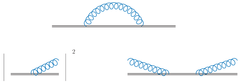
Figure 4.5: Schematic decomposition of a one-loop jet propagator (with an internal soft gluon) into its real and imaginary parts. In the main text, we use this as a device to give some intuition behind the transverse scattering rate and the asymptotic mass. Note that one of the gluons needs to be soft in order to give a non-zero contribution to the scattering rate; a cut through two hard gluons would yield a kinematically impossible process.

4.4 Classical corrections to Jet Quenching

We proceed to demonstrate the power of the tools that have been introduced in the previous sections through a computation of the LO soft contribution to the transverse scattering rate, $\mathcal{C}(k_{\perp})$, which was introduced in Sec. 3.2 as well as the LO soft contribution to the asymptotic mass, $m_{\infty}$.

It will nevertheless be insightful to first consider the top diagram from Fig.4.5, representing the one-loop correction to a quark or gluon jet propagator, where the blue gluon represents an HTL propagator. By separating the imaginary and real parts of that diagram, we can schematically distinguish two kinds of jet-medium interactions:

• By the optical theorem, the imaginary part of the top diagram from Fig.4.5 is given by cutting through the loop in that diagram, putting the cut propagators on-shell and then squaring the process defined by the cut, as is shown in Fig.4.5 - bottom left. This a true scattering process, one where the jet actually exchanges transverse momentum with a medium constituent and these kinds of effects are captured by the transverse scattering rate. In the Wilson loop picture, which will be introduced shortly, Fig.4.5 - bottom left can be thought of as corresponding to Fig. 4.7 - left.

• Conversely, Fig.4.5 - bottom right corresponds to forward scattering. Scattering off a medium constituent causes the jet to temporarily changes direction before it scatters again, forcing it back into its original momentum state, which induces a phase shift. It is this phase shift that induces a dispersion correction, otherwise known as the asymptotic mass. For the case of a quark jet, there is an additional diagram not shown in Fig. 4.5 with the quark line cut.

Such a distinction should shed some light on the form of Eq. 3.29. There, the imaginary part of the Hamiltonian contains the interaction terms. Having provided some intuition using the points made above, we are now ready to start on the leading order calculations of $\mathcal{C}(k_{\perp}),\,m_{\infty}$. We take this opportunity to explain the various calculational steps in some detail as many such manoeuvres will be used throughout Chs. 5 and  6.

4.4.1 Leading Order Soft Contribution to $\mathcal{C}(k_{\perp})$

We wish to compute the transverse scattering rate associated with a parton passing through a medium of constant length $L_{M}$. As was done throughout the previous chapter, the parton is assumed to propagate eikonally in the $x^{+}$ direction with momentum $P=(E,0,0)$ and $E\gg T$, the temperature of the plasma.

The route of our computation begins by looking at the expectation value of the Wilson loop [285, 286, 287], defined in the $x^{-}=0$ plane as

$$\langle W(x_{\perp})\rangle=\frac{1}{N_{c}}\Tr\langle[0,x_{\perp}]_{-}\mathcal{W}^{\dagger}(x_{\perp})[x_{\perp},0]_{+}\mathcal{W}(0)\rangle,,$$ (4.90)

where the trace is over colour. The parton’s eikonal nature allows us to describe its propagation with the Wilson line $\mathcal{W}$ (the horizontal lines in Fig. 4.6), which incorporates an infinite number of gluon exchanges between the parton and the medium

$$\mathcal{W}(x_{\perp})=\mathcal{P}\exp\Big(ig\int_{-\frac{L_{M}}{2}}^{\frac{L_{M}}{2}}dx^{+}A^{-}(x^{+},x_{\perp})\Big{missing}).$$ (4.91)

In order to preserve gauge invariance the “side rails” also need to be included [287]

$$[x_{\perp},y_{\perp}]_{\pm}=\mathcal{P}\exp\Big(-ig\int_{1}^{0}ds(y_{\perp}-x_{\perp})\cdot A_{\perp}(\pm\frac{L_{M}}{2},x_{\perp}+(y_{\perp}-x_{\perp})s)\Big{missing}),$$ (4.92)

although in non-singular gauges, they will not contribute. The fields in the Wilson loop are to be understood as transforming in the representation, $R$ of the jet particle and as path-ordered. Thus, in rough analogy with Fig. 3.3, one may think of the eikonalised hard quark in the amplitude as $\mathcal{W}(0)$ and $\mathcal{W}^{\dagger}(x_{\perp})$ as its conjugate-amplitude counterpart. The zero-subtracted Fourier transform of $\mathcal{C}_{R}(k_{\perp})$, defined in Eq. (3.22) is then obtained by expanding

$$\lim_{L_{M}\to\infty}\langle W(x_{\perp})\rangle=\exp(-\mathcal{C}_{R}(x_{\perp})L_{M})$$ (4.93)

in $g$. In order to declutter notation, we remove the $R$ subscript, i.e $\mathcal{C}(k_{\perp})\equiv\mathcal{C}_{R}(k_{\perp})$ and do the same for its Fourier transform. Similarly, $\hat{q}(\mu_{\perp})\equiv\hat{q}_{R}(\mu_{\perp})$ (unless otherwise stated).

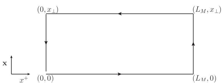
Figure 4.6: Wilson line from Eq. (4.90). The horizontal lines can be interpreted as the hard parton in the amplitude (bottom) and the conjugate amplitude (top). The side rails are inserted for the sake of maintaining gauge invariance but will not contribute in, for instance, the Coulomb gauge. The small gap in the bottom left corner of the Wilson loop in Fig. 4.6 is intended to emphasise that the trace is over colour only; the fields themselves cannot be moved using the cyclicity of the trace. Reproduced from [284].

Schematically, we expect such an expansion to have the following structure

$$\lim_{L_{M}\to\infty}\langle W(x_{\perp})\rangle=1-\left(\mathcal{C}_{\text{LO}}(x_{\perp})+\mathcal{C}_{\text{NLO}}(x_{\perp})+...\right)L_{M}+\frac{\left(\mathcal{C}_{\text{LO}}(x_{\perp})+\mathcal{C}_{\text{NLO}}(x_{\perp})+...\right)^{2}}{2}L_{M}^{2}+...$$ (4.94)

where the $\mathcal{C}_{\text{NLO}}$ term (in the vacuum) is suppressed by $\mathcal{O}(g^{2})$ compared to $\mathcal{C}_{\text{LO}}$. By expanding $\lim_{L_{M}\to\infty}\langle W(x_{\perp})\rangle$ in $g$, we can then read off $\mathcal{C}(x_{\perp})$ to whatever order we are interested in, by looking at the coefficient multiplying $L_{M}$ in Eq. (4.94). See App. B for a discussion on how to expand $\mathcal{W}$, while properly taking care of path-ordering.

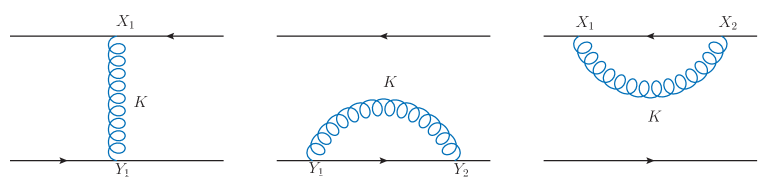
Figure 4.7: Three diagrams contributing to $\mathcal{C}(x_{\perp})$ at LO. The lower Wilson line is time-ordered, admitting only type “1” vertices whereas the lower one is anti-time-ordered and admits only type “2” vertices. In lightcone coordinates $X_{1}=(x_{1}^{+},0,\mathbf{x}),\,X_{2}=(x_{2}^{+},0,\mathbf{x})$ and $Y_{1}=(y_{1}^{+},0,0)$. We colour the exchanged gluon as blue in order to denote that it is soft, i.e its momenta is $K\sim gT$ and thus must be described with an HTL propagator.

Starting from Eq. (4.93), we recover three terms at the first non-trivial order, corresponding to the three diagrams in Fig. 4.7. We denote the leftmost diagram as “real” and the other two “virtual”. From left to right they read, respectively

$$g^{2}C_{R}\int_{-\frac{L_{M}}{2}}^{\frac{L_{M}}{2}}dx_{1}^{+}\int_{-\frac{L_{M}}{2}}^{\frac{L_{M}}{2}}dy_{1}^{+} \langle A^{-}(x_{1}^{+},x_{\perp})A^{-}(y^{+},0)\rangle$$

$$=g^{2}C_{R}\int_{-\frac{L_{M}}{2}}^{\frac{L_{M}}{2}}dx_{1}^{+}\int_{-\frac{L_{M}}{2}}^{\frac{L_{M}}{2}}dy_{1}^{+}\int_{K}e^{-ik^{-}(x_{1}^{+}-y_{1}^{+})}e^{i\mathbf{k}\cdot\mathbf{x}}G_{>}^{--}(k),$$ (4.95)

$$-g^{2}C_{R}\int_{-\frac{L_{M}}{2}}^{\frac{L_{M}}{2}}dy_{2}^{+}\int_{-\frac{L_{M}}{2}}^{y_{2}^{+}}dy_{1}^{+} \langle A^{-}(y_{2}^{+},0)A^{-}(y_{1}^{+},0)\rangle$$

$$=-g^{2}C_{R}\int_{-\frac{L_{M}}{2}}^{\frac{L_{M}}{2}}dy_{2}^{+}\int_{-\frac{L_{M}}{2}}^{y_{2}^{+}}dy_{1}^{+}\int_{K}e^{-ik^{-}(y_{2}^{+}-y_{1}^{+})}G_{F}^{--}(k),$$ (4.96)

$$-g^{2}C_{R}\int_{-\frac{L_{M}}{2}}^{\frac{L_{M}}{2}}dx_{2}^{+}\int_{-\frac{L_{M}}{2}}^{x_{2}^{+}}dx_{1}^{+} \langle A^{-}(x_{1}^{+},x_{\perp})A^{-}(x_{2}^{+},x_{\perp})\rangle$$

$$=-g^{2}C_{R}\int_{-\frac{L_{M}}{2}}^{\frac{L_{M}}{2}}dx_{2}^{+}\int_{-\frac{L_{M}}{2}}^{x_{2}^{+}}dx_{1}^{+}\int_{K}e^{-ik^{-}(x_{2}^{+}-x_{1}^{+})}G_{\tilde{F}}^{--}(k).$$ (4.97)

Before combining the three terms, it is useful to rewrite the first one

$$\text{Eq.}\eqref{eq:realterm} =g^{2}C_{R}\int_{-\frac{L_{M}}{2}}^{\frac{L_{M}}{2}}dx_{1}^{+}\int_{-\frac{L_{M}}{2}}^{\frac{L_{M}}{2}}dy_{1}^{+}\int_{K}e^{-ik^{-}(x_{1}^{+}-y_{1}^{+})}e^{i\mathbf{k}\cdot\mathbf{x}}G_{>}^{--}(k)\Big{(}\Theta(x_{1}^{+}-y_{1}^{+})+\Theta(y_{1}^{+}-x_{1}^{+})\Big{)}$$

$$=g^{2}C_{R}\Big{[}\int_{-\frac{L_{M}}{2}}^{\frac{L_{M}}{2}}dx_{1}^{+}\int_{-\frac{L_{M}}{2}}^{x_{1}^{+}}dy_{1}^{+}\int_{K}e^{-ik^{-}(x_{1}^{+}-y_{1}^{+})}e^{i\mathbf{k}\cdot\mathbf{k}}G_{>}^{--}(k)$$

$$+\int_{-\frac{L_{M}}{2}}^{\frac{L_{M}}{2}}dy_{1}^{+}\int_{-\frac{L_{M}}{2}}^{y^{+}_{1}}dx_{1}^{+}\int_{K}e^{-ik^{-}(x_{1}^{+}-y_{1}^{+})}e^{i\mathbf{k}\cdot\mathbf{x}}G_{>}^{--}(k)\Big{]}$$

$$=g^{2}C_{R}\Big{[}\int_{-\frac{L_{M}}{2}}^{\frac{L_{M}}{2}}dx_{1}^{+}\int_{-\frac{L_{M}}{2}}^{x_{1}^{+}}dy_{1}^{+}\int_{K}e^{-ik^{-}(x_{1}^{+}-y_{1}^{+})}e^{i\mathbf{k}\cdot\mathbf{x}}G_{>}^{--}(k)$$

$$+\int_{-\frac{L_{M}}{2}}^{\frac{L_{M}}{2}}dy_{1}^{+}\int_{-\frac{L_{M}}{2}}^{y^{+}_{1}}dx_{1}^{+}\int_{K}e^{-ik^{-}(x_{1}^{+}-y_{1}^{+})}e^{i\mathbf{k}\cdot\mathbf{x}}G_{>}^{--}(k)\Big{]}$$ (4.98)

The second term above then can be combined with the first by relabelling $x_{1}^{+}\to y_{1}^{+},y_{1}^{+}\to x_{1}^{+}$ and using invariance in the transverse plane. Upon adding Eqs. (4.98),  (4.96) and  (4.97), we obtain

$$\mathcal{C}(x_{\perp})_{\text{LO}}L_{M}=2g^{2}C_{R}\int_{K}(1-e^{i\mathbf{k}\cdot\mathbf{x}})\int_{-\frac{L_{M}}{2}}^{\frac{L_{M}}{2}}dx_{1}^{+}\int_{-\frac{L}{2}}^{x_{1}^{+}}dy_{1}^{+}e^{-ik^{-}(x_{1}^{+}-y_{1}^{+})}G^{--}_{rr}(k),$$ (4.99)

where we have also used Eq. (4.55). In order to make the position integration converge, we need to add a small imaginary part to $k^{-}$ so that the exponential decays for $x_{1}^{+}\gg y_{1}^{+}$, i.e

$$\int_{-\frac{L_{M}}{2}}^{\frac{L_{M}}{2}}dx_{1}^{+}\int_{-\frac{L_{M}}{2}}^{x_{1}^{+}}dy_{1}^{+}e^{-i(k^{-}-i\varepsilon)(x_{1}^{+}-y_{1}^{+})} =\int_{-\frac{L_{M}}{2}}^{\frac{L_{M}}{2}}dx_{1}^{+}\frac{-i}{k^{-}-i\varepsilon}$$

$$=\frac{-i}{k^{-}-i\varepsilon}L_{M},$$ (4.100)

where we have neglected the term with $e^{-\varepsilon L_{M}}$ factor. This yields, for the scattering kernel in position space

$$\mathcal{C}(x_{\perp})_{\text{LO}}=2g^{2}C_{R}\int_{\mathbf{k}}(1-e^{i\mathbf{k}\cdot\mathbf{x}})\int\frac{dk^{+}dk^{-}}{(2\pi)^{2}}\frac{-i}{k^{-}-i\varepsilon}G^{--}_{rr}(k).$$ (4.101)

Using Eq. (3.22), we can then easily read off $\mathcal{C}(k_{\perp})$. Indeed, since the contribution from real diagrams always multiply the factor $e^{i\mathbf{k}\cdot\mathbf{x}}$ in $\mathcal{C}(x_{\perp})$, it is only necessary to compute the real diagrams in order to extract $\mathcal{C}(k_{\perp})$; the $x_{\perp}$-independent term contributes to probability conservation. We will make use of this simplification throughout Ch. 5.

Using $G_{rr}(K)$ is even in $K$ we then get

$$\mathcal{C}(k_{\perp})_{\text{LO}}=2\pi g^{2}C_{R}\int\frac{dk^{+}dk^{-}}{(2\pi)^{2}}\delta(k^{-})\left(\frac{1}{2}+n_{\text{B}}(k^{0})\right)\rho_{\text{B}}^{--}(K).$$ (4.102)

At this stage, we can deduce from the presence of the statistical function that $\mathcal{C}(k_{\perp})_{\text{LO}}$ receives classical contributions. These classical contributions originate from the $gT$ and $g^{2}T$ scales where the exchange of gluons between the jet and the medium has a large occupation number . Such a condition is satisfied when the exchanged gluon has energy $\ll T$ so that the statistical function can be approximated as $n_{\text{B}}(k^{0})\approx T/k^{0}\gg 1$.

We additionally assume that $k_{\perp}\gtrsim gT$. This is then the exact scaling associated with the gluon exchanges that dominate the multiple scattering regime (see Sec. 3.2).

As was discussed in Sec. 4.2.4 propagators with soft momenta running through them must be described by HTL propagators, which resum an infinite number of internal hard thermal loops. Going back to Eq. (4.102), we can make use of the ideas from Sec. 4.3, shifting $k^{z}\rightarrow k^{z}+k^{0}$

$$\mathcal{C}(k_{\perp})_{\text{LO}}=g^{2}C_{R}\int\frac{dk^{0}}{(2\pi)}\left(\frac{1}{2}+n_{\text{B}}(k^{0})\right)\rho_{\text{B}}^{--}(K)\Big{|}_{k^{z}=0}.$$ (4.103)

The analytical properties of $G_{rr}^{--}(K)$ in the $k^{0}$ plane effectively allow us to let $k^{0}\rightarrow i\omega_{n}$ and trade $\int dk^{0}/2\pi\to iT\sum_{n}$, where we recall that the sum is over the Matsubara modes with $\omega_{n}=2\pi nT$ and the definitions of the HTL propagators (in Coulomb gauge) from Eqs. (4.72), (LABEL:htltrans)

$$\mathcal{C}(k_{\perp})_{\text{LO}} =iTg^{2}C_{R}\sum_{n}\bigg{(}\frac{i}{-\omega_{n}^{2}+k_{\perp}^{2}+m_{D}^{2}\left(1-\frac{i\omega_{n}}{2\sqrt{-\omega_{n}^{2}+k_{\perp}^{2}}}\ln\frac{i\omega_{n}+\sqrt{-\omega_{n}^{2}+k_{\perp}^{2}}}{i\omega_{n}-\sqrt{-\omega_{n}^{2}+k_{\perp}^{2}}}\right)}$$

$$+\frac{k_{\perp}^{2}}{-\omega_{n}^{2}+k_{\perp}^{2}}\frac{i}{-\omega_{n}^{2}-k_{\perp}^{2}-\frac{m_{D}^{2}}{2}\left(\frac{-\omega_{n}^{2}}{-\omega_{n}^{2}+k_{\perp}^{2}}-\left(\frac{-\omega_{n}^{2}}{-\omega_{n}^{2}+k_{\perp}^{2}}+1\right)\frac{i\omega_{n}}{2\sqrt{-\omega_{n}^{2}+k_{\perp}^{2}}}\ln\frac{i\omega_{n}+\sqrt{-\omega_{n}^{2}+k_{\perp}^{2}}}{i\omega_{n}-\sqrt{-\omega_{n}^{2}+k_{\perp}^{2}}}\right)}\bigg{)}.$$ (4.104)

Given that we are only interested in the soft contribution, we may discard all but the zero mode

$$\mathcal{C}(k_{\perp})_{\text{LO}}=Tg^{2}C_{R}\bigg{(}-\frac{1}{k_{\perp}^{2}+m_{D}^{2}}+\frac{1}{k_{\perp}^{2}}\bigg{)}=\frac{g^{2}TC_{R}m_{D}^{2}}{k_{\perp}^{2}(k_{\perp}^{2}+m_{D}^{2})}.$$ (4.105)

Reassuringly, we have recovered Eq. (3.24), which was first calculated by Aurenche, Gelis and Zakaret [168] using a sum rule. Assuming the transverse momentum is cut off such that $T\gg\mu_{\perp}\gg m_{D}$, we then arrive at the LO soft contribution to the transverse momentum broadening coefficient, $\hat{q}(\mu_{\perp})$ with the use of Eq. (3.43), which immediately yields Eq. (3.46). In Ch. 5, we will will build on this result by calculating double logarithmic corrections to $\hat{q}(\mu_{\perp})$.

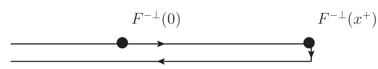
Figure 4.8: Pictoral depiction of the Wilson line in Eq. (4.108). Reading Eq. (4.108) from right to left, the lightlike Wilson line starts at $x^{\prime+}=-\infty$, with $F^{-\perp}$ insertions at $x^{\prime+}=0$ and $x^{\prime+}=x^{+}$ before being brought back to $x^{\prime+}=-\infty$.

4.4.2 Leading Order Soft Contribution to $Z_{g}$

We have seen that the asymptotic mass, $m_{\infty}$ appears as a shift in the hard parton’s dispersion relation due to forward scattering with the medium. Through Eq. (4.76), we moreover understand how the masses can be computed in terms of $Z_{g}$ and $Z_{f}$. At leading order, they both receive a contribution from the scale, $T$

$$Z_{f}^{\text{LO}} =\frac{T^{2}}{12},$$ (4.106)

$$Z_{g}^{\text{LO}} =\frac{T^{2}}{6}.$$ (4.107)

At $\mathcal{O}(g)$, $Z_{g}$ then gets a contribution from the soft scale, $gT$. The purpose of this section will be to show how this contribution can be computed using the Wilson line lying along the lightcone

$$Z_{g}=\frac{1}{d_{R}C_{R}}\int_{0}^{\infty}dx^{+}\,x^{+}\Tr\langle U_{R}(-\infty;x^{+})v_{\mu}F^{\mu\nu}(x^{+})U_{R}(x^{+};0)v_{\rho}F^{\rho}_{\nu}(0)U_{R}(0;-\infty)\rangle.$$ (4.108)

where

$$U_{R}(x^{+};0)=\mathcal{P}\;\exp\left(ig\int_{0}^{x^{+}}dy^{+}A^{-a}(y^{+})T^{a}_{R}\right)$$ (4.109)

Per our discussion in Sec. 4.3, these kinds of corrections are suitable for calculation in EQCD. We choose here to instead compute it using HTL theory, as it will nicely set up the calculation in full QCD that will follow in Ch. 6.

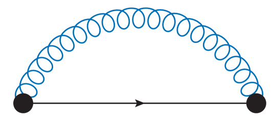
Figure 4.9: Diagram contributing to $Z_{g}$ at NLO. In keeping with our convention, the blue gluon is soft and therefore needs to be represented with an HTL propagator.

Expanding Eq. (4.108) to first order in $g$, we find (see App. A for our conventions with respect to lightcone coordinates)

$$Z_{g}^{\text{NLO}}=-2\int_{0}^{\infty}dx^{+}\,x^{+}\left\langle(\partial^{-}A^{x}(x^{+},0,0)-\partial^{x}A^{-}(x^{+},0,0))(\partial^{-}A^{x}(0,0,0)-\partial^{x}A^{-}(0,0,0))\right\rangle,$$ (4.110)

where we have used invariance in the transverse plane to write $F^{-x}F^{-x}+F^{-y}F^{-y}=2F^{-x}$. Being sandwiched between two 1 vertices, the relevant gluon propagator should be a time-ordered $G_{F}$. However, from using that $x^{+}\geq 0$ and Eq. (4.53), we understand that we can just as well work with $G_{>}$

$$Z_{g}^{\text{NLO}} =-2\int_{0}^{\infty}dx^{+}\int_{K}x^{+}e^{-ik^{-}x^{+}}(k^{-2}G_{>}^{xx}(K)-2k^{x}k^{-}G_{>}^{x-}(K)+{k^{x}}^{2}G_{>}^{--}(K))$$

$$=2\int_{K}\frac{1}{(k^{-}-i\epsilon)^{2}}(k^{-2}G_{>}^{xx}(K)-2k^{x}k^{-}G_{>}^{x-}(K)+{k^{x}}^{2}G_{>}^{--}(K))$$

$$=2\int_{K}\frac{1+n_{\text{B}}(k^{0})}{(k^{-}-i\epsilon)^{2}}(k^{-2}(G_{R}^{xx}(K)-G_{A}^{xx}(K))-2k^{x}k^{-}(G_{R}^{x-}(K)-G_{A}^{x-}(K))$$

$$+{k^{x}}^{2}(G_{R}^{--}(K)-G_{A}^{--}(K)))$$

$$=2\int_{K}\frac{1+n_{\text{B}}(k^{0})}{(k^{-}-i\epsilon)^{2}}(F_{R}(K)-F_{A}(K))$$ (4.111)

where

$$F_{R/A}(K) =k^{-2}G^{xx}_{R/A}(K)-2k^{x}k^{-}\Big{(}G^{0x}_{R/A}(K)-G^{zx}_{R/A}(K)\Big{)}$$

$$+{k^{x}}^{2}\Big{(}G^{00}_{R/A}(K)+G^{zz}_{R/A}(K)-2G^{z0}_{R/A}(K)\Big{)},$$ (4.112)

and the causal HTL propagators are given in the Feynman gauge in Eq. (4.78). The pesky $1/(k^{-}-i\epsilon)^{2}$ factor makes it so that we cannot immediately trade the $k^{0}$ integral for a Matsubara sum, as was done in Eq. (4.104). Instead, we must first do shift i.e $k^{z}\rightarrow k^{z}+k^{0}$. Then we can let $k^{0}\rightarrow i\omega_{n}$, trading the frequency integral for a sum over the Matsubara modes. Since we are once again only interested in the soft contribution, we are permitted to only keep zero mode term, which leaves us with

$$Z_{g}^{\text{NLO}}=T\int_{k}\frac{1}{(k^{z}+i\varepsilon)^{2}}\left(\frac{2{k^{z}}^{2}}{k^{2}}-\frac{k_{\perp}^{2}}{k^{2}+m_{D}^{2}}+\frac{k_{\perp}^{2}}{k^{2}}\right).$$ (4.113)

In DR, because they are scaleless, the first and third terms do not contribute. Integrating the second term yields

$$Z_{g}^{\text{NLO}}=-\frac{Tm_{D}}{2\pi},$$ (4.114)

a negative correction with respect to Eq. (4.106). We interpret this as representing a reduction in the thermal mass due to the screening of infrared gauge modes.

4.4.3 Non-Perturbative Determination of Classical Corrections

To conclude this chapter, we provide a brief discussion on the program inspired by the ideas [11] laid out in Sec. 4.3, that is, to determine using lattice EQCD corrections to $\mathcal{C}(k_{\perp})$ and $Z_{g}$.

A flurry of papers [288, 289, 12, 13] on the computation non-perturbative (NP) determination of $\mathcal{C}(k_{\perp})$ have emerged in the last decade or so. This effort has culminated with the complete determination [14] of the NP kernel and its impact on the in-medium splitting rate.

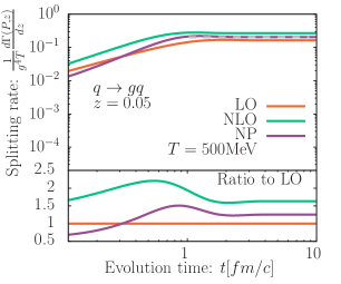
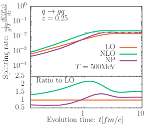
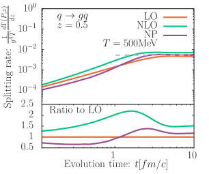
Figure 4.10: Comparison of non-perturbative determination of in-medium splitting with both LO and NLO kernel, evolved in time. Figures taken directly from [14].

In that paper, the NP scattering rate is essentially used as input for Eq. (3.41), suitably generalised to deal with a medium of finite length (see [159]), whose solution, obtained numerically is then used to calculate the in-medium splitting rate. This is what is shown in Fig. 4.10 as a function of time for $3$ different values of splitting fraction $z$ (note that we called the splitting fraction $x$ in Ch. 3). In particular, the solution with the NP kernel is compared to the LO kernel and the NLO kernel, computed in [11]. We point out that for certain values of the parameter space, the NP kernel can be $50\%$ larger than the LO value, implying that these higher-order corrections have the potential to be quantitatively impactful. An eventual goal, which we have started working towards in [18], to be detailed in the next chapter, is to understand how these NP corrections to $\mathcal{C}(k_{\perp})$ (or equivalently, $\hat{q}(\mu)$) compete with the logarithmically enhanced corrections coming in at the next order in $g$.

An effort to determine the NP corrections to $Z_{g}$ has largely progressed in parallel [15, 16] to the NP calculation of $\mathcal{C}(k_{\perp})$, as much of the technology developed for the lattice computation is directly applicable to both cases. However, extracting the NP correction is not as simple as just blindly computing Eq.(4.108) on the lattice. For one, as detailed in [15] it is not possible to integrate Eq.(4.108) up to arbitrarily large $x^{+}$ since at some point, the signal-to-noise ratio from the numerical integration stifles a robust determination of the correlator. To overcome this issue, for large separations the correlator data must be fitted to a model, based on the expected exponential faloff from electrostatic and magnetostatic screening. Another issue is the high energy behaviour of Eq. (4.108); at some point the lattice determination becomes limited by lattice spacing and discretisation effects. Fortunately however, it is in this (short distance) region where a perturbative EQCD calculation should in principle agree with the lattice determination. In this way, one must perform a matching procedure to fix the short-distance evaluation of the NP corrections.

Furthermore, since EQCD possesses divergences for energies approaching the thermal scale, one needs to check that those UV divergences cancel against corresponding IR divergences coming from full QCD. This latter step has already been completed for $\mathcal{C}(k_{\perp})$ but remains to be done for $Z_{g}$ and will compose the majority of Ch. 6’s material. Indeed, the perturbative EQCD calculation in [16] does not include such a matching onto the 4D theory; they subtract off the divergent EQCD behaviour from their results. The following schematic equation, taken from [16] should help to set the stage for the calculation to be done in that chapter, where the different rows correspond to the order in $g$ at which the corrections are present.

$$\hphantom{\bigg{[}\quad}\mathrm{scale\;}T \mathrm{scale\;}gT \mathrm{scale\;}g^{2}T$$

$$Z_{g}= \bigg{[}\quad\frac{T^{2}}{6}-\frac{T\mu_{\text{h}}}{\pi^{2}} \bigg{]}$$

$$+ \bigg{[}\quad -\frac{Tm_{\text{D}}}{2\pi}+\frac{T\mu_{\text{h}}}{\pi^{2}} \bigg{]}$$

$$+ \bigg{[}\quad c^{\ln}_{\text{hard}}\ln\frac{T}{\mu_{\text{h}}}+c_{\text{T}} +c^{\ln}_{\text{hard}}\ln\frac{\mu_{\text{h}}}{m_{\text{D}}}+c^{\ln}_{\text{soft}}\ln\frac{m_{\text{D}}}{\mu_{\text{s}}}+c_{gT} +c^{\ln}_{\text{soft}}\ln\frac{\mu_{\text{s}}}{g^{2}T}+c_{gT^{2}} \bigg{]}$$

$$+ \,\mathcal{O}(g^{3})\;.$$ (4.115)

In the first row, there is only a contribution from the scale $T$, which we have previously written down in Eq. (4.106). In the second row, there is only a classical contribution, which we calculated using HTL theory in the previous section (see Eq. (4.114)). In that calculation, we did not recover the part of the correction depending on the cutoff, $\mu_{\text{h}}$, which cancels against the same correction but with opposite sign at LO. This is indeed consistent with our previous assertation that such corrections are never found when using DR as a regulator.

At $\mathcal{O}(g^{2})$, there are contributions from the hard, soft and ultrasoft scales. In Ch. 6, we will essentially focus on calculating the $c^{\ln}_{\text{hard}}\ln T/\mu_{\text{h}}$ and $c_{\text{T}}$ terms, showing that the former cancels against the term $c^{\ln}_{\text{hard}}\ln\mu_{\text{h}}/m_{\text{D}}$, which was calculated in [16]. Since we will use DR there, these logarithmic divergences will show up as $1/\epsilon$ poles. The NP determination of $Z_{g}$ will then be able to stand on its own, void of any divergences. Our long-term goal is then to calculate the entire $\mathcal{O}(g^{2})$ from the scale $T$, which, along with its $Z_{f}$ counterpart will allow for the complete evaluation of the asymptotic mass’ $\mathcal{O}(g^{2})$ corrections.

Something which has not been made so clear up this point is why we need not worry about further matching between the EQCD and full QCD at higher orders in $g$. The answer to this question is provided by the fact that EQCD is a super-renormalisable theory; if one demands that quantities be cut off in the UV by $\mu_{\text{h}}$, at each order in $g$, the corrections will go as a different power of $\mu_{\text{h}}$. In other words, we can expect the UV behaviour at $\mathcal{O}(g^{n})$ to be $\mu_{\text{h}}^{2-n}$ so that after the leading linear and subleading logarithmic divergences, we only produce negative powers in the UV cutoff.

Chapter 5 Quantum Corrections to Jet Broadening

In Caron-Huot’s original work [11] where he computed the $\mathcal{O}(g)$ correction to $\hat{q}(\mu_{\perp})$, he anticipated the potential presence of corrections at one further order in $g$ coming from gluons that are collinear to the hard parton. Indeed, in computing $\hat{q}(\mu_{\perp})$ to $\mathcal{O}(g^{2})$, one starts to encounter diagrams corresponding to radiative corrections [218, 1, 2]; in contrast to the LO calculation in Sec. 4.4.1 where just a soft gluon is exchanged with the medium, diagrams here also contain bremsstrahlung and are shown in Fig. 5.1. The authors [1, 2] showed that these corrections possess double logarithmic and single logarithmic enhancements, where the argument of the double logarithm was found to be $L_{M}/\tau_{\text{min }}$ with $L_{M}$ the length of the medium and $\tau_{\text{min}}\sim 1/T$ an IR cutoff to be elucidated further upon discussion.

While the original calculations concretely demonstrated the presence of these (logarithmic) corrections, they did not strive to quantify their arguments precisely. Although difficult, the latter goal is of paramount importance, as it of course controls whether the logarithms are large compared to the factor of $g^{2}$ that precedes them and the (non-perturbatively calculated) classical corrections that start to come in at $\mathcal{O}(g)$. It has been argued in both papers [1, 2] that the double logarithmic corrections are sourced from the single-scattering regime, where this bremsstrahlung is triggered by a single, harder scattering between the jet and the medium. By tackling this problem using TFT, we will be able to rigorously judge and furthermore quantify how the thermal scale is relevant for these corrections.

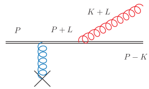
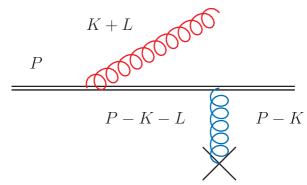
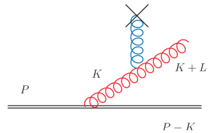
Figure 5.1: Diagrams contributing to radiative momentum broadening in the single-scattering regime. The double solid line represents the hard jet parton (quark or gluon), curly lines are gluons and the cross is a quark or gluon scattering centre in the medium.

The approach of [2] makes clear that these corrections arise from taking into account the recoil during the medium-induced emission of a gluon. There, evolution equations describing medium-induced gluon splitting are derived and studied. Additional terms in these equations coming from keeping track of the transverse momentum that the jet picks up from the medium are then interpreted as corrections to $\hat{q}(\mu{\perp})$.

While both of these calculations arrive at essentially the same conclusions, we choose to instead sketch the calculation done in [1]. We make contact between this calculation and our Wilson loop setup, introduced in Sec. 4.4.1, showing how we can reproduce their result. From there, we explore the neighbouring regions of phase space and in doing so, identify which of them have the potential to possess double logarithmic enhancements. The chapter closes with a demonstration of how the double-logarithmic region of phase space is situated with respect to the region from which the classical corrections [11] emerge. A strict use of Coulomb gauge is adopted throughout this chapter.

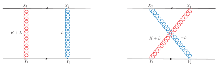
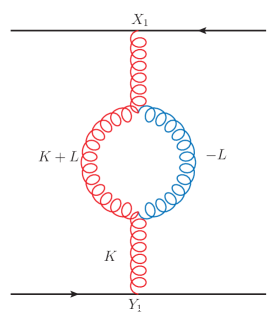
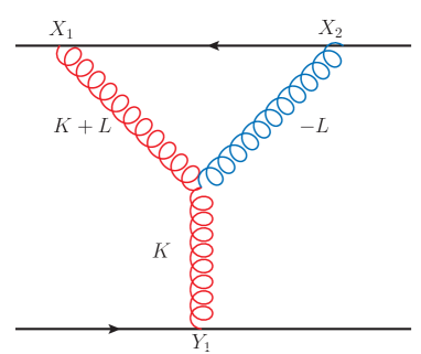
Figure 5.2: Diagrams giving rise to the single-scattering regime. The two horizontal solid lines are the Wilson lines $\mathcal{W}$. Red gluons are coft, representing bremsstrahlung while the blue ones are HTL-resummed and soft. See the main text for the precise scalings. Momenta flow from bottom to top.

This chapter is based on the work [18].

5.1 Wilson Loop Setup at $\mathcal{O}(g^{2})$

In this section we will build upon the groundwork laid in Sec. 4.4.1, demonstrating how our Wilson loop setup can be applied to compute higher order corrections to $\mathcal{C}(k_{\perp})$ and hence $\hat{q}({\mu_{\perp}})$. It turns out that the diagrams from Fig. 5.2 are the ones that we will need to compute in order to capture the aforementioned double logarithmic corrections. Therefore, a good place to start is to try and understand how these diagrams correspond to those shown in Fig. 5.1 – the single scattering processes.

As was also the case for the LO evaluation, the horizontal black lines in Fig. 5.2 are respectively $\mathcal{W}$ and $\mathcal{W}^{\dagger}$ Wilson lines representing the hard jet parton in the amplitude and conjugate amplitude. In our setup, the $\mathcal{W}$ ($\mathcal{W}^{\dagger}$) line corresponds to a hard jet parton with initial (final) momentum $P=(E,0,0)$ with $E\gg T$, the temperature of the plasma. The gluons exchanged with the medium are, as before, soft and thus are HTL-resummed. The red gluons denote collinear bremsstrahlung that is harder than the blue gluons but still soft in comparison to the leading jet parton. Borrowing the terminology of [290], we call these modes “coft”. They are instead described by bare propagators. We concretely define the coft scaling here, for general four-momentum

$$Q\sim\tilde{\lambda}E(1,\lambda^{2},\lambda)\quad\quad\lambda,\tilde{\lambda}\ll 1$$ (5.1)

This scaling naturally incorporates the collinearity (with respect to the jet axis) of the radiation as well as the fact that its $+$ component is much smaller than the energy, $E$ of the jet. We hold off on choosing explicit scales from $\lambda,\,\tilde{\lambda}$ until a later point. Calculations are always set up so that the cut coft propagator has momentum $K+L$ and the HTL one momentum $L$. In this way, $K$ is always the momentum exchanged between the two Wilson lines.

But how can we interpret these diagrams in terms of those shown in Fig. 5.1. Well, cuts are understood to go horizontally through the middle of each diagram in Fig. 5.2. It then transpires that the first top two diagrams in Fig. 5.2 correspond to the square of the top two in Fig. 5.1 and their interference. The bottom left diagram in Fig. 5.2 corresponds to the square of the bottom in Fig. 5.1. Finally the bottom right in Fig. 5.2 corresponds to the interference of the top two with the bottom one in Fig. 5.1.

Still, it is perhaps not clear why there are only $4$ diagrams in Fig. 5.2 as opposed to $6$. This apparent discrepancy can be clarified by re-examining Eq. (4.94), which we repeat here for convenience

$$\lim_{L_{M}\to\infty}\langle W(x_{\perp})\rangle=1-\left(\mathcal{C}_{\text{LO}}(x_{\perp})+\mathcal{C}_{\text{NLO}}(x_{\perp})+...\right)L_{M}+\frac{\left(\mathcal{C}_{\text{LO}}(x_{\perp})+\mathcal{C}_{\text{NLO}}(x_{\perp})+...\right)^{2}}{2}L_{M}^{2}+...\,.$$ (5.2)

It emerges that only two-particle irreducible (2PI) diagrams appear in the coefficient of $L_{M}$ above, implying that they are the only class of diagrams that we need consider [291, 292] in order to compute $\mathcal{C}_{\text{NNLO}}(x_{\perp})$ and hence $\mathcal{C}_{\text{NNLO}}(k_{\perp})$. Other diagrams appear in higher order terms in the $L_{M}$ expansion.

This naturally begs the question: why are we considering the two-particle reducible top left diagram of Fig. 5.2? To this end, note that the colour factor associated with this diagram, which we denote as II to reflect its topology is given as

$$C_{\text{II}}=\frac{1}{N_{c}}\Tr[T^{b}T^{d}T^{c}T^{a}]\delta^{ab}\delta^{cd}=\frac{1}{N_{c}}\Tr[T^{a}T^{a}T^{c}T^{c}]=C_{R}^{2},$$ (5.3)

where the prefactor of $1/N_{c}$ comes from Eq. (4.90) and the generators are in the representation $R$ of $\text{SU}(N_{c})$ under which the hard parton transforms. The colour factor of the diagram to its right, which we denote as X possesses a non-Abelian piece

$$C_{\text{X}}=\frac{1}{N_{c}}\Tr[T^{d}T^{b}T^{c}T^{a}]\delta^{ab}\delta^{cd}=\frac{1}{N_{c}}\Tr[(T^{a}T^{c}+[T^{c},T^{a}])T^{c}T^{a}]=C_{R}^{2}-\frac{C_{R}C_{A}}{2}.$$ (5.4)

It is precisely this non-abelian piece that survives once we add the two diagrams together, as we will now see. In order to clean up the notation, we write $\delta\mathcal{C}=\mathcal{C}^{\text{log}}_{\text{NNLO}}$ so that by using Eqs. (4.90),  (4.91) and the expansion in terms of the scattering kernel, we arrive at

$$\delta\mathcal{C} (x_{\perp})^{\text{\cal{R}}}_{\mathrm{II+X}}=-2g^{4}\int_{-\frac{L_{M}}{2}}^{\frac{L_{M}}{2}}dx_{2}^{+}\int_{-\frac{L_{M}}{2}}^{\frac{L_{M}}{2}}dx_{1}^{+}\int_{-\frac{L_{M}}{2}}^{\frac{L_{M}}{2}}dy_{2}^{+}\int_{-\frac{L_{M}}{2}}^{\frac{L_{M}}{2}}dy_{1}^{+}G_{>}^{--}(x_{1}^{+}-y_{1}^{+},x_{\perp})G_{>}^{--}(x_{2}^{+}-y_{2}^{+},x_{\perp})\times$$

$$\times\Theta(y_{2}^{+}-y_{1}^{+})\Bigg{(}C_{R}^{2}\Theta(x_{2}^{+}-x_{1}^{+})+\Big{(}C_{R}^{2}-\frac{C_{R}C_{A}}{2}\Big{)}\Theta(x_{1}^{+}-x_{2}^{+})\Bigg{)}$$

$$=-2g^{4}\int_{-\frac{L_{M}}{2}}^{\frac{L_{M}}{2}}dx_{2}^{+}\int_{-\frac{L_{M}}{2}}^{\frac{L_{M}}{2}}dx_{1}^{+}\int_{-\frac{L_{M}}{2}}^{\frac{L_{M}}{2}}dy_{2}^{+}\int_{-\frac{L_{M}}{2}}^{\frac{L_{M}}{2}}dy_{1}^{+}G_{>}^{--}(x_{1}^{+}-y_{1}^{+},x_{\perp})G_{>}^{--}(x_{2}^{+}-y_{2}^{+},x_{\perp})\times$$

$$\times\Theta(y_{2}^{+}-y_{1}^{+})\Bigg{(}-\frac{C_{R}C_{A}}{2}\Theta(x_{1}^{+}-x_{2}^{+})+C_{R}^{2}\Bigg{)}$$ (5.5)

where we have added a factor of $2$ in front to account for the diagrams where the scalings are inverted. In addition, the R superscript specifies that we have included the contribution from real diagrams. As was discussed in Sec. 4.4.1, real diagrams are the only ones needed in order to determine $\delta\mathcal{C}(k_{\perp})$ and hence $\delta\hat{q}(\mu_{\perp})$. Both propagators are of type $>$ because they are stretching from the bottom Wilson line, which only admits “1” vertices to the top one, which only admits “2” vertices.

Coming back to the expression above, it is interesting to observe that, upon symmetrising the term proportional to $C_{R}^{2}$ in $x_{1}\leftrightarrow x_{2}\,,\,y_{1}\leftrightarrow y_{2}$ and then adding them, we arrive at

$$\frac{1}{2}g^{4}C_{R}^{2}\int_{-\frac{L}{2}}^{\frac{L}{2}}dx_{1}^{+}\int_{-\frac{L}{2}}^{\frac{L}{2}}dy_{1}^{+}G^{--}_{>}(x_{1}^{+}-y_{1}^{+},x_{\perp})\int_{-\frac{L}{2}}^{\frac{L}{2}}dx_{2}^{+}\int_{-\frac{L}{2}}^{\frac{L}{2}}dy_{2}^{+}G^{--}_{>}(x_{2}^{+}-y_{2}^{+},x_{\perp}),$$ (5.6)

which is indeed the square of the (real) diagram computed in Sec. 4.4.1; the position integrals will give an $L_{M}^{2}$ factor, signifying that this diagram is part of the exponentiation of the tree-level contribution. In any case, the term proportional to $C_{R}^{2}$ will inevitably be forced to vanish due to the presence of a $\delta\left(\left(\mathbf{k}+\mathbf{l}\right)^{2}+m_{\infty}^{2}\right)$ in the coft propagator, signalling that this process is kinematically impossible.

To briefly summarise, we have argued that even though diagram II does not contribute to $\delta\mathcal{C}(k_{\perp})$, it cancels the abelian piece of diagram X, leaving us with only a non-abelian contribution. For the other diagrams in Fig. 5.2, we will not need to consider these kinds of extra diagrams, since their contributions do not possess an additional abelian piece.

Getting back to the matter at hand, one can do the position integrals and extract

$$\delta\mathcal{C}(k_{\perp})_{\mathrm{II+X}} =C_{R}C_{A}g^{4}\int\frac{dk^{+}dk^{-}}{(2\pi)^{2}}\int_{L}\frac{1}{(l^{-}-i\epsilon)^{2}}G_{>}^{--}(K+L)G_{>}^{--}(-L)2\pi\delta(k^{-}).$$ (5.7)

A factor of 2 has been added to account for the inverted scaling. The $\delta(k^{-})$ arises from the $x^{+}$ integrations, which essentially enforce the eikonalised hard parton to remain on-shell after the emission. We postpone continuing with the evaluation of this diagram until the next section, where we assume specific scalings for $K,\,L$.

We now proceed to the self-energy diagram on the bottom left in Fig. 5.2. Its contribution reads

$$\delta\mathcal{C}(k_{\perp})_{\mathrm{self}}=g^{4}C_{R}C_{A}\int\frac{dk^{+}}{2\pi}\int_{L}G_{R}^{-\rho}(K)\Big{(}g_{\gamma\sigma}(2L{+}K)_{\rho}-g_{\sigma\rho}(2K{+}L)_{\gamma}+g_{\rho\gamma}(K{-}L)_{\sigma}\Big{)}$$

$$\times G_{>}^{\sigma\delta}(K+L)G_{>}^{\gamma\alpha}(-L)\Big{(}g_{\delta\beta}(2K{+}L)_{\alpha}-g_{\alpha\delta}(2L{+}K)_{\beta}-g_{\alpha\beta}(K{-}L)_{\delta}\Big{)}G_{A}^{\beta-}(K)\Big{|}_{k^{-}=0}.$$ (5.8)

Cuts going through the $K$ propagators are again vanishing, hence their retarded/advanced assignments only, which is consistent with the cutting rules for Wightman functions [17, 166].

Finally, the Y-shaped diagram on the bottom right of Fig. 5.2, together with its symmetry-related counterparts yield

$$\delta\mathcal{C}(x_{\perp})^{\text{\cal{R}}}_{\mathrm{Y}}= 2g^{4}C_{R}C_{A}\int\frac{dk^{+}d^{2}k_{\perp}}{(2\pi)^{3}}\int_{L}\frac{i}{l^{-}+i\epsilon}e^{i\mathbf{k}\cdot\mathbf{x}}G_{>}^{-\delta}(K+L)G_{>}^{-\alpha}(-L)$$

$$\hskip 34.14322pt\times\Big{(}g_{\alpha\delta}(2L+K)_{\beta}-g_{\delta\beta}(2K+L)_{\alpha}+g_{\beta\alpha}(K-L)_{\delta}\Big{)}G_{F}^{\beta-}(K)\Big{|}_{k^{-}=0}.$$ (5.9)

At this point, it is useful to write the Feynman propagator as

$$G_{F}(K)=\frac{1}{2}\Big{(}G_{R}(K)+G_{A}(K)\Big{)}+G_{rr}(K).$$ (5.10)

Since $G_{rr}$ is the average of the bare cut propagators and we have already set $k^{-}=0$, it vanishes. That leaves us with the average of the retarded and advanced bare Green’s functions, which when evaluated at $k^{-}=0$ are the same. We can then extract, as was done with the previous diagrams

$$\delta\mathcal{C}(k_{\perp})_{\mathrm{Y}}= -2g^{4}C_{R}C_{A}\int\frac{dk^{+}}{2\pi}\int_{L}\frac{i}{l^{-}+i\epsilon}G_{>}^{-\delta}(K+L)G_{>}^{-\alpha}(-L)$$

$$\hskip 34.14322pt\times\Big{(}g_{\alpha\delta}(2L+K)_{\beta}-g_{\delta\beta}(2K+L)_{\alpha}+g_{\beta\alpha}(K-L)_{\delta}\Big{)}G_{R}^{\beta-}(K)\Big{|}_{k^{-}=0}.$$ (5.11)

We find this to be a good stopping point for the evaluation of these diagrams. The computation will be resumed following a brief review of the calculation from [1], which will shed some light on how we can enforce single scattering kinematics, allowing us to assign precise scalings to the momenta $K,\,L$.

5.2 Double Logarithms from [1, 2]

In [1], the double logarithmic corrections to $\hat{q}(\mu_{\perp})$ emerge through the use of the standard dipole formalism [293]

$$\delta\mathcal{C}(k_{\perp})^{\mathcal{N}=1}=4\alpha_{s}C_{R}\int\frac{dk^{+}}{k^{+}}\int^{\rho_{\perp}}\frac{d^{2}l_{\perp}}{(2\pi)^{2}}\mathcal{C}_{\text{LO}}(l_{\perp})\frac{l_{\perp}^{2}}{k_{\perp}^{2}(\mathbf{k}+\mathbf{l})^{2}},$$ (5.12)

where $l_{\perp}^{2}/(k_{\perp}^{2}(\mathbf{k}+\mathbf{l})^{2})$ is the standard dipole factor and $2C_{R}/k^{+}$ the soft limit of the $g\leftarrow R$ DGLAP splitting function. Finally, $\mathcal{C}_{\text{LO}}(l_{\perp})$ is the leading order scattering rate from a gluon source.

Eq. (5.12) is in principle just the first, $N=1$ term in the opacity expansion (see Secs. 3.5,  3.6.2). Within Eq. (5.12), we can identify the leading order value of the transverse momentum broadening coefficient i.e

$$\hat{q}_{\text{LO}}(\rho_{\perp})=\int^{\rho_{\perp}}\frac{d^{2}l_{\perp}}{(2\pi)^{2}}l_{\perp}^{2}\mathcal{C}_{\text{LO}}(l_{\perp}).$$ (5.13)

Neglecting the dependence on the UV cutoff, $\rho_{\perp}$, thereby setting $\hat{q}_{\text{LO}}(\rho_{\perp})\rightarrow\hat{q}_{0}$ effectively enforces the Harmonic Oscillator Approximation. In addition, as observed in [1], the requirement that the transverse momentum carried away by the bremsstrahlung is larger than that picked up in a typical collision with the medium, $|\mathbf{k}+\mathbf{l}|\gg l_{\perp}$, implements single scattering kinematics, where the $\mathcal{N}=1$ term dominates the expansion. This leaves us with

$$\delta\mathcal{C}(k_{\perp})_{\text{\cite[cite]{[\@@bibref{Number}{Liou:2013qya,Blaizot:2013vha}{}{}]}}}=4\alpha_{s}C_{R}\hat{q}_{0}\int\frac{dk^{+}}{k^{+}}\frac{1}{k_{\perp}^{4}}.$$ (5.14)

Taking the second moment (with respect to $k_{\perp}$) will then give us the correction to $\hat{q}(\mu_{\perp})$ that we desire

$$\delta\hat{q}_{\text{\cite[cite]{[\@@bibref{Number}{Liou:2013qya,Blaizot:2013vha}{}{}]}}}(\mu_{\perp})=4\alpha_{s}C_{R}\hat{q}_{0}\int^{\mu}\frac{d^{2}k_{\perp}}{k_{\perp}^{2}}\int\frac{dk^{+}}{k^{+}}.$$ (5.15)

It is clear from above how the double logarithm emerges – one comes from the collinear $d^{2}k_{\perp}/k_{\perp}^{2}$ divergence and the other comes from the soft $dk^{+}/k^{+}$ divergence. This explains why, at the level of our Wilson loop computation, bremsstrahlung possesses coft scaling.

For the sake of convenience, we choose to integrate over the formation time, $\tau=k^{+}/k_{\perp}^{2}$ instead of $k_{\perp}$. The integration limits, which bound the triangle shown in Fig. 5.3 are then [1]:

• $\tau<\sqrt{k^{+}/\hat{q}_{0}}$, represented by line $(b)$ in Fig. 5.3. In the deep LPM regime, $k_{\perp}^{2}\sim\hat{q}_{0}\tau_{\text{LPM}}$. The former constraint then emerges upon demanding that $\tau<k_{\perp}^{2}/\hat{q}_{0}$ and solving for $\tau$. Effectively, this prevents the formation time from getting sufficiently large to lead us into the multiple scattering regime, which will cut off the double-logarithmic phase space: the collinear $dk_{\perp}^{2}/k_{\perp}^{2}$ log can exist as long as the initial and final states can propagate along straight lines for sufficiently long times before and after the single scattering [161].

• $\tau>k^{+}/\mu_{\perp}^{2}$, represented by line $(a)$. This condition on the formation time corresponds to enforcing the UV cutoff on transverse momentum, i.e. $k_{\perp}<\mu_{\perp}$. In the original derivation of [1] this $\mu_{\perp}$ cutoff is identified with the saturation scale $Q_{s}^{2}\equiv\hat{q}_{0}L_{M}$. If instead $\mu_{\perp}>Q_{s}$ the boundaries of the double-logarithmic region change, as shown in [219].

• $\tau>\tau_{\text{min}}$, represented by line $(c)$. This IR cutoff $\tau_{\text{min}}$ is intended to render the end result finite. The motivation for this boundary comes from requiring that the duration of the single scattering does not become comparable to the formation time of the radiated gluon, as the former is treated as instantaneous within the collinear-radiation framework. In [1, 2] this duration was assumed to be proportional to the inverse temperature, leading to $\tau_{\text{min}}\sim 1/T$. We will return to this assumption in the next section.

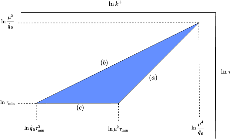
Figure 5.3: Schematic depiction of the bounds on the integral in Eq.. The $(b)$ side of the triangle is given by $\tau=\sqrt{k^{+}/\hat{q}_{0}}$ whereas the $(a)$ one is given by $\tau=k^{+}/\mu_{\perp}^{2}$. The logarithmic axes allow one to easily read the result of the integral Eq. (5.16) straight from the figure, up to the prefactor $\alpha_{s}C_{R}\hat{q}_{0}/\pi$. Our labelling for the three boundaries follows that of [1].

Adding these limits explicitly,

$$\delta\hat{q}_{\text{\cite[cite]{[\@@bibref{Number}{Liou:2013qya,Blaizot:2013vha}{}{}]}}}(\mu_{\perp})=\frac{\alpha_{s}C_{R}}{\pi}\hat{q}_{0}\int_{\tau_{\text{min}}}^{\mu_{\perp}^{2}/\hat{q}_{0}}\frac{d\tau}{\tau}\int_{\hat{q}_{0}\tau^{2}}^{\mu_{\perp}^{2}\tau}\frac{dk^{+}}{k^{+}},$$ (5.16)

the double-logarithmic correction,

$$\delta\hat{q}_{\text{\cite[cite]{[\@@bibref{Number}{Liou:2013qya,Blaizot:2013vha}{}{}]}}}(\mu_{\perp})=\frac{\alpha_{s}C_{R}}{\pi}\hat{q}_{0}\ln^{2}\frac{\mu_{\perp}^{2}}{\hat{q}_{0}\tau_{\text{min}}}$$ (5.17)

immediately follows. This is the form of [2]; that of [1] arises by choosing $\mu^{2}_{\perp}=\hat{q}_{0}L_{M}$, so that the argument of the double logarithm becomes the familiar $L_{M}/\tau_{\text{min}}$. The single-logarithmic corrections arising from a more sophisticated analysis of the regions neighbouring the three boundaries of the triangle shown in Fig. 5.3 have been presented in [1].

5.3 Adapting [1, 2] Corrections to a Weakly Coupled QGP

The double-logarithmic phase space we just sketched, as per [1, 2], is derived for a medium described by a random color field with a non-zero two-point function for the $A^{-}$ component, i.e.

$$\left\langle A^{-a}(\mathbf{q},x^{+})A^{-b}(\tilde{\mathbf{q}},\tilde{x^{+}})\right\rangle=\delta^{ab}\delta(x^{+}-\tilde{x}^{+})n(x^{+})(2\pi)^{2}\delta^{(2)}(\mathbf{q}-\tilde{\mathbf{q}})\frac{g^{4}}{q_{\perp}^{4}}$$ (5.18)

This corresponds for instance to the time-honoured parameterisation of a medium of static scattering centres of density $n$ and is consistent with modelling the medium with the GW kernel, Eq. (3.54). However, a weakly coupled QGP contains more medium effects than those captured by these instantaneous, space-like interactions; in particular, as soon as the light-cone frequency ($k^{+}$) range overlaps with the temperature scale, one needs to account for the Bose-Einstein stimulated emission of the radiated gluon and, at negative $k^{+}$, for the absorption of a gluon from the medium. We could naively account for these effects by amending Eq. (5.16) into

$$\delta\hat{q}(\mu_{\perp})=\frac{\alpha_{s}C_{R}}{\pi}\hat{q}_{0}\int_{\tau_{\text{min}}}^{\mu_{\perp}^{2}/\hat{q}_{0}}\frac{d\tau}{\tau}\int_{\hat{q}_{0}\tau^{2}}^{\mu_{\perp}^{2}\tau}\frac{dk^{+}}{k^{+}}\left(1+2n_{\text{B}}(k^{+})\right).$$ (5.19)

The factor of two in Eq. (5.19) accounts for stimulated emission and for absorption, which has been reflected in the positive-frequency range.

Let us now perform a careful, parametric analysis of Fig. 5.3, taking into account some relevant timescales listed in Table. 5.1, in order to probe the robustness of the $\tau_{\text{min}}\sim 1/T$ assumption, made by the authors in [1, 2]. In doing so, we come across some potential issues:

• This choice of $\tau_{\text{min}}$ is consistent for the rarer, harder exchanges between the jet and medium but fails for softer scatterings, which take place over a longer duration. In particular, the duration-dependent nature of the IR cutoff seems rather troubling.

• We also note that, for frequencies parametrically smaller than the temperature, which $\tau_{\text{min}}\sim 1/T$ allows, the bottom-left corner of the triangle becomes ill-defined, since one can have $\sqrt{k^{+}/\hat{q}_{0}}<1/g^{2}T$.

• Furthermore, the factorisation into soft and collinear logarithms undergirding Eq. (5.16) is predicated on a collinear expansion $k^{+}\gg k_{\perp}$, i.e. $\tau k^{+}\gg 1$ [220]. This $\ln\tau>-\ln k^{+}$ line in principle excludes parts of Fig. 5.3: the $(b)-(c)$ vertex is below it, since $\hat{q}_{0}\tau_{\text{min}}^{3}\sim g^{4}\ll 1$ for $\tau_{\text{min}}\sim 1/T$. The exclusion stretches to the $\ln\tau=-\ln k^{+}$ line, which crosses lines $(c)$ and $(b)$ if $\mu_{\perp}\tau_{\text{min}}>1$, i.e. $\mu_{\perp}>T$. If instead $\mu_{\perp}<T$, it crosses lines $(a)$ and $(b)$.

Can the issues above be addressed by going back to Eq. (5.16) and adapting the limits there or do we need to include the statistical function, as in Eq. (5.19)? If $T$ is much smaller than the lower boundary on the energy integration, which from Fig. 5.3 is $\hat{q}_{0}\tau_{\text{min}}^{2}$, then the statistical function will be exponentially suppressed and we will of course recover Eq. 5.17. We have thus sharpened the previous question: is $\hat{q}_{0}\tau_{\text{min}}^{2}\gg T$ or rather $\tau_{\text{min}}\gg\sqrt{T/\hat{q}_{0}}\sim 1/(g^{2}T)$ consistent with single scattering?

Quantity	Parametric Dependence	Symbol
Hard scattering duration	$1/T$	–
Soft scattering duration	$1/(gT)$	–
Soft scattering mean free time	$1/(g^{2}T)$	$t_{\text{el}}$
LO $\hat{q}(\mu_{\perp})$ in HOA	$g^{4}T^{3}$	$\hat{q}_{0}$
LPM formation time	$\gtrsim 1/(g^{2}T)$	$\tau_{\text{LPM}}$

Table 5.1: Some timescales associated with a weakly coupled QGP. By hard scattering, we mean $2\to 2$ exchange between the jet and medium, which exchange momentum $\sim T$. By soft scattering, we mean $2\to 2$ exchange between the jet and medium, which exchamge momentum $\sim gT$.

Well, $t_{\text{el}}\sim 1/g^{2}T$ is the mean free time between the frequent soft, $k_{\perp}\sim gT$ scattering between the jet and medium constituents. The resummation of these scatterings on this $1/g^{2}T$ timescale makes it so that $\tau\gtrsim 1/g^{2}T$ in the multiple scattering regime, thus answering negatively our previous question. Moreover, in what is to follow, we identify a strict single-scattering regime, also giving rise to double-logarithmic corrections, where the formation time is a priori $\tau\ll 1/g^{2}T$. We can therefore conclude that it is not reasonable to put such a demand on $\tau_{\text{min}}$ and that the $k^{+}$ integral in Eq. (5.19) should run over the thermal scale.

Furthermore, our position is that the definition of single-scattering from [1, 2] is not exclusively that of a single scattering: the collinear divergence gets cut off when $k_{\perp}$ becomes small enough ($\tau$ large enough) that multiple scatterings start to contribute within a formation time, and that this happens before entering the deep LPM regime. However, at double-logarithmic accuracy one cannot distinguish between a $k_{\perp}^{2}\gg\hat{q}_{0}\tau$ and a $k_{\perp}^{2}\sim\hat{q}_{0}\tau$ boundary, and in the HOA, one cannot disentangle multiple soft scatterings from a single harder one.

To shed some light on the issues raised above, our strategy is the following: we introduce an intermediate regulator $\tau_{\text{int}}$, with $1/gT\ll\tau_{\text{int}}\ll 1/g^{2}T$. The lower boundary will be discussed soon, whereas the upper boundary makes it so that for $\tau>\tau_{\text{int}}$ we thus include parts of the strict single scattering regime, as well as the “few scatterings” regime just mentioned. We can then rewrite Eq. (5.19) with the new integration boundaries, which we have argued in favour of

$$\delta\hat{q}(\mu_{\perp})^{\mathrm{few}}=\frac{\alpha_{s}C_{R}}{\pi}\hat{q}_{0}\int_{\tau_{\text{int}}}^{\mu_{\perp}^{2}/\hat{q}_{0}}\frac{d\tau}{\tau}\int_{\hat{q}_{0}\tau^{2}}^{\mu_{\perp}^{2}\tau}\frac{dk^{+}}{k^{+}}\left(1+2n_{\text{B}}(k^{+})\right).$$ (5.20)

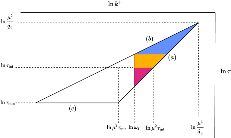
Figure 5.4: A pictorial representation of how the phase space of the radiated gluon is partitioned once thermal effects are taken into account. See the main text for the explanation of the different subregions.

To calculate Eq. (5.20), the additional complication that we need to overcome (with respect to the calculation of Eq. (5.16)) is dealing with the statistical function in the $k^{+}$ integrand. In order to demonstrate how this can be done, let us for the moment consider the integral $\int_{\nu_{\text{IR}}}^{\nu_{\text{UV}}}dk^{+}n_{\text{B}}(k^{+})/k^{+}$ with $\nu_{\text{UV}}\gg T\gg\nu_{\text{IR}}$. The idea is then to introduce an intermediate regulator, $\epsilon$ in the spirit of dimensional regularisation

$$\int^{\nu_{\text{UV}}}_{\nu_{\text{IR}}}\frac{dk^{+}}{k^{+}}n_{\text{B}}(k^{+}) =\lim_{\epsilon\to 0}\left[\int^{\nu_{\text{UV}}}_{0}\frac{dk^{+}}{k^{+}}k^{+\epsilon}n_{\text{B}}(k^{+})-\int^{\nu_{\text{IR}}}_{0}\frac{dk^{+}}{k^{+}}k^{+\epsilon}n_{\text{B}}(k^{+})\right]$$

$$=\lim_{\epsilon\to 0}\left[\int^{\infty}_{0}\frac{dk^{+}}{k^{+}}k^{+\epsilon}n_{\text{B}}(k^{+})-\int^{\nu_{\text{IR}}}_{0}\frac{dk^{+}}{k^{+}}k^{+\epsilon}\left(\frac{T}{k^{+}}-\frac{1}{2}\right)\right]+\mathcal{O}\left(\frac{\nu_{\text{IR}}}{T},e^{-\frac{\nu_{\text{UV}}}{T}}\right)$$

$$=\lim_{\epsilon\to 0}\left[T^{\epsilon}\zeta(\epsilon)\Gamma(\epsilon)-\left(\frac{T\nu_{\text{IR}}^{\epsilon}}{\nu_{\text{IR}}(\epsilon-1)}-\frac{\nu_{\text{IR}}^{\epsilon}}{2\epsilon}\right)\right]+\mathcal{O}\left(\frac{\nu_{\text{IR}}}{T},e^{-\frac{\nu_{\text{UV}}}{T}}\right)$$

$$=\frac{T}{\nu_{\text{IR}}}+\frac{1}{2}\ln\frac{\nu_{\text{IR}}e^{\gamma_{E}}}{2\pi T}+\mathcal{O}\left(\frac{\nu_{\text{IR}}}{T},e^{-\frac{\nu_{\text{UV}}}{T}}\right)\,.$$ (5.21)

The main advantage is that it allows us to use the known analytically-continued integrations of the Bose–Einstein distribution in terms of the Riemann $\zeta$ and Euler $\Gamma$ functions. Moreover, we take this opportunity to define the thermal scale $\omega_{T}\equiv 2\pi T\exp(-\gamma_{E})$ with $\gamma_{E}$ the Euler–Mascheroni constant.

In terms of Eq. (5.20), let us look at the thermal part first, i.e

$$\int_{\tau_{\text{int}}}^{\frac{\mu_{\perp}^{2}}{\hat{q}_{0}}}\frac{d\tau}{\tau}\int_{\hat{q}_{0}\tau^{2}}^{\mu_{\perp}^{2}\tau}\frac{dk^{+}}{k^{+}}n_{\text{B}}(k^{+})=\int_{\hat{q}_{0}\tau_{\text{int}}^{2}}^{\mu_{\perp}^{2}\tau_{\text{int}}}\frac{dk^{+}}{k^{+}}n_{\text{B}}(k^{+})\int_{\tau_{\text{int}}}^{\sqrt{\frac{k^{+}}{\hat{q}_{0}}}}\frac{d\tau}{\tau}+\int^{\frac{\mu_{\perp}^{4}}{\hat{q}_{0}}}_{\mu_{\perp}^{2}\tau_{\text{int}}}\frac{dk^{+}}{k^{+}}n_{\text{B}}(k^{+})\int_{\frac{k^{+}}{\mu_{\perp}^{2}}}^{\sqrt{\frac{k^{+}}{\hat{q}_{0}}}}\frac{d\tau}{\tau}.$$ (5.22)

In our $\hat{q}_{0}\tau_{\text{int}}^{2}\ll\omega_{T}\ll\mu_{\perp}^{2}\tau_{\text{int}}$ hierarchy, the second integral is exponentially suppressed. For the first one, we can proceed as follows

$$\int_{\hat{q}_{0}\tau_{\text{int}}^{2}}^{\mu_{\perp}^{2}\tau_{\text{int}}}\frac{dk^{+}}{k^{+}}n_{\text{B}}(k^{+})\int_{\tau_{\text{int}}}^{\sqrt{\frac{k^{+}}{\hat{q}_{0}}}}\frac{d\tau}{\tau}=\frac{1}{2}\int_{\hat{q}_{0}\tau_{\text{int}}^{2}}^{\mu_{\perp}^{2}\tau_{\text{int}}}\frac{dk^{+}}{k^{+}}n_{\text{B}}(k^{+})\ln\frac{k^{+}}{\hat{q}_{0}\tau_{\text{int}}^{2}}.$$ (5.23)

We can then exploit that

$$\int_{0}^{\infty}\frac{dk^{+}}{k^{+}}k^{+\epsilon}n_{\text{B}}(k^{+})\ln\frac{k^{+}}{T}=T^{\epsilon}\Gamma(\epsilon)\left(\zeta^{\prime}(\epsilon)+\zeta(\epsilon)\psi(\epsilon)\right),$$ (5.24)

where $\psi(x)$ is the digamma function. This, together with Eq. (5.21), leads to

$$\int_{\hat{q}_{0}\tau_{\text{int}}^{2}}^{\mu_{\perp}^{2}\tau_{\text{int}}}\frac{dk^{+}}{k^{+}}n_{\text{B}}(k^{+})\int_{\tau_{\text{int}}}^{\sqrt{\frac{k^{+}}{\hat{q}_{0}}}}\frac{d\tau}{\tau}= \frac{T}{2\hat{q}_{0}\tau_{\text{int}}^{2}}+\frac{1}{8}\left(-\ln^{2}\frac{\omega_{T}}{\hat{q}_{0}\tau_{\text{int}}^{2}}+\gamma_{E}^{2}-\frac{\pi^{2}}{4}+2\gamma_{1}\right)$$

$$+\mathcal{O}\left(\frac{\hat{q}_{0}\tau_{\text{int}}^{2}}{T},e^{-\frac{\mu_{\perp}^{2}\tau_{\text{int}}}{T}}\right),$$ (5.25)

which in turn can be added to the straightforward vacuum part to give

$$\delta\hat{q}(\mu_{\perp})^{\mathrm{few}}=\frac{\alpha_{s}C_{R}}{2\pi}\hat{q}_{0}\bigg{\{}\frac{2T}{\hat{q}_{0}\tau_{\text{int}}^{2}}+\ln^{2}\frac{\mu_{\perp}^{2}}{\hat{q}_{0}\tau_{\text{int}}}-\frac{1}{2}\ln^{2}\frac{\omega_{T}}{\hat{q}_{0}\tau_{\text{int}}^{2}}+\frac{\gamma_{E}^{2}}{2}-\frac{\pi^{2}}{8}+\gamma_{1}+\ldots\bigg{\}}.$$ (5.26)

At double-logarithmic accuracy, we then have

$$\delta\hat{q}(\mu_{\perp})_{\mathrm{dlog}}^{\mathrm{few}}=\frac{\alpha_{s}C_{R}}{2\pi}\hat{q}_{0}\bigg{\{}\ln^{2}\frac{\mu_{\perp}^{2}}{\hat{q}_{0}\tau_{\text{int}}}-\frac{1}{2}\ln^{2}\frac{\omega_{T}}{\hat{q}_{0}\tau_{\text{int}}^{2}}\bigg{\}}\quad\text{with}\;\frac{\omega_{T}}{\mu_{\perp}^{2}}\ll\tau_{\text{int}}\ll\sqrt{\frac{\omega_{T}}{\hat{q}_{0}}}.$$ (5.27)

Graphically, if we take $k^{+}=\omega_{T}$ as a vertical line in Fig. 5.4, the first term in Eq. (5.27) comes from integrating over the entire “1+2” triangle, whereas the second term comes from subtracting the smaller 2 triangle, which therefore does not contribute to double-logarithmic accuracy. Furthermore, this $k^{+}=\omega_{T}$ line intersects line $(b)$ at $\sqrt{\omega_{T}/\hat{q}_{0}}\sim 1/g^{2}T$, thus excluding the range where the formation time estimate becomes unreliable.

We also remark that, for $\tau_{\text{int}}>\tau_{\text{min}}$, the horizontal $\tau=\tau_{\text{int}}$ line intersects the diagonal sides of the triangle at $k^{+}=\hat{q}_{0}\tau_{\text{int}}^{2}$ (line $(b)$) and $k^{+}=\mu_{\perp}^{2}\tau_{\text{int}}$ (line $(a)$). The form (5.27) arises when the temperature scale $\omega_{T}$ falls in between these two values, so that $\hat{q}_{0}\tau_{\text{int}}^{2}\ll\omega_{T}\ll\mu_{\perp}^{2}\tau_{\text{int}}$, resulting in the range of validity expressed there.

This is where the size of $\mu_{\perp}$ with respect to the medium scales enters. At leading order, i.e. without considering these radiative corrections, choosing $gT\ll\mu_{\perp}\ll T$ ensures that only the contributions of the soft modes [168] are included, whereas $T\ll\mu_{\perp}$ also includes the thermal-mode contribution [174]. If we allow for radiative corrections and further require a strict single-scattering contribution, we shall show that $\mu_{\perp}\gg\sqrt{g}T$ is necessary, so as to include the so-called semi-collinear processes of [283, 294]. Finally, $\frac{\omega_{T}}{\mu_{\perp}^{2}}\ll\tau_{\text{int}}$ should be complemented by the duration bound $\tau_{\text{int}}\gg\tau_{\text{min}}$: for $\mu_{\perp}\ll T$ this is automatically satisfied, whereas for $\mu_{\perp}\gtrsim T$ it will then be a further constraint to be imposed. In other words, for $\mu_{\perp}<\sqrt{\omega_{T}/\tau_{\text{min}}}\sim T$ the vertical $k^{+}=\omega_{T}$ line intersects boundaries $(b)$ and $(a)$, whereas for $\mu_{\perp}>\sqrt{\omega_{T}/\tau_{\text{min}}}\sim T$ it would intersect $(b)$ and $(c)$.

We assume $\sqrt{g}T\ll\mu_{\perp}\ll T$ for all remaining sections in this chapter, except for Sec. 5.5.

5.4 Double Logarithmic Corrections from the Wilson Loop Setup

To briefly recapitulate, in Sec. 5.2 we described how the double logarithmic corrections to $\hat{q}(\mu_{\perp})$ were calculated in [1], taking care to highlight the boundaries of the region of phase space that those authors argued should give rise to these corrections. Whereas that calculation was done for a medium characterised by a random colour field, we showed in Sec. 5.3 how, for the case of a dynamical medium, one can and in fact, one must account for contributions from the thermal scale.

We resume here the computation started in Sec. 5.1. Our plan is then to show how the latter result can be obtained through our setup, while also arguing in favour of the necessity to include corrections from an additional region of phase space, which we coin the strict single-scattering regime. To start, we draw on what we have learned regarding the nature of the double logarithmic enhancements in the previous sections to specify scalings for the coft and soft propagators introduced in Sec. 5.1.

In order to ensure that the energy integration runs over the thermal scale, we let $\tilde{\lambda}=T/E$. Taking $\lambda=\sqrt{g}$ then fixes the transverse component to $\sim\sqrt{g}T$ (see footnote 9) so that

$$(K+L)\sim(T,gT,\sqrt{g}T).$$ (5.28)

Before specifying the $L$ scaling, let us go back to the computation of $\delta\mathcal{C}(k_{\perp})=\delta\mathcal{C}(k_{\perp})_{\mathrm{II+X}}+\delta\mathcal{C}(k_{\perp})_{\text{self}}+\delta\mathcal{C}(k_{\perp})_{\mathrm{Y}}$ in Sec. 5.1. Once the Lorentz algebra is done, the coft propagator appears in all of the diagrams as

$$G^{--}_{>}(K+L)=G^{L}_{>}(K+L)+\frac{(\mathbf{k}+\mathbf{l})^{2}}{(\vec{\mathbf{k}}+\vec{\mathbf{l}})^{2}}G^{T}_{>}(K+L).$$ (5.29)

In Coulomb gauge, the longitudinal component of the (bare) coft propagator vanishes. The transverse component then reads, expanded in $g$, assuming Eq. (5.28) and that $k^{+}\gg l^{+}$

$$G_{>}^{T}(K+L) =2\pi\varepsilon(k^{+}+l^{+})\Big{(}1+n_{\text{B}}(k^{+}+l^{+})\Big{)}\delta((K+L)^{2}-m_{\infty}^{2})\bigg{|}_{k^{-}=0}$$

$$\approx 2\pi\varepsilon(k^{+})\Big{(}1+n_{\text{B}}(k^{+})\Big{)}\frac{\delta(l^{-}-\frac{(\mathbf{k}+\mathbf{l})^{2}+m_{\infty}^{2}}{2k^{+}})}{2\absolutevalue{k^{+}}},$$ (5.30)

where $\varepsilon(x)$ is $1$ for $x>0$ and $-1$ for $x<0$. Upon implementing the single scattering condition, $k_{\perp}\gg l_{\perp}$ highlighted in Sec. 5.2

$$G_{>}^{T}(K+L)\sim 2\pi\varepsilon(k^{+})\Big{(}1+n_{\text{B}}(k^{+})\Big{)}\frac{\delta(l^{-}-\frac{k_{\perp}^{2}}{2k^{+}})}{2\absolutevalue{k^{+}}}.$$ (5.31)

Presented like this, the delta function suggests the interpretation of $l^{-}\sim gT$ as an inverse formation time. Moreover, the smallest momentum that can be acquired from the medium through a single scattering is, at LO $l_{\perp}\sim gT$, which, in turn, fixes $l^{+}\sim gT$. The scaling of the soft modes thus read

$$L\sim(gT,gT,gT).$$ (5.32)

It has been shown that the interaction of the coft and soft modes give rise to so-called [283, 294] semi-collinear processes. These semi-collinear processes contribute to regions $3$ and $4$ in Fig. 5.4, which make up the strict single scattering regime. Here, the characteristic formation time, $1/l^{-}\sim gT$ overlaps with the duration of the soft, $l_{\perp}\sim gT$ scattering.

We can now add contributions from the three diagrams, i.e Eqs. (5.7),  (5.8) and  (5.11) before expanding the combination in the scaling that we have just motivated to get

$$\delta\mathcal{C}(k_{\perp})_{\text{semi}} =2g^{4}C_{R}C_{A}\int\frac{dk^{+}}{2\pi}\int\frac{d^{4}L}{(2\pi)^{3}}\Big{(}1+n_{\text{B}}(k^{+})\Big{)}\frac{\delta(l^{-}-\frac{k_{\perp}^{2}}{2k^{+}})}{k_{\perp}^{4}k^{+}}\frac{T}{l^{+}+\frac{l^{-}}{2}}\Bigg{(}l_{\perp}^{2}\rho^{--}(l)$$

$$+2\rho^{T}(l)\Big{(}{l^{-}}^{2}-\frac{l^{+}l^{-}l_{\perp}^{2}}{l^{2}}\Big{)}\Bigg{)}.$$ (5.33)

In this scaling where $l^{+}\sim gT$ is soft, we only need to keep the zero mode contribution. We are therefore permitted to make use of the ideas discussed in Sec. 4.3; the $l^{+}$ integrand has after all already been encountered in the calculation of the LO scattering rate in Sec. 4.4.1 . Doing the $l^{+}$ integration yields

$$\delta\mathcal{C}(k_{\perp})_{\text{semi}} =2g^{4}C_{R}C_{A}T\int\frac{dk^{+}}{2\pi}\int\frac{d^{2}l_{\perp}}{(2\pi)^{2}}\int dl^{-}\Big{(}1+n_{\text{B}}(k^{+})\Big{)}\frac{\delta(l^{-}-\frac{k_{\perp}^{2}}{2k^{+}})}{k_{\perp}^{4}k^{+}}$$

$$\times\Bigg{(}-\frac{l_{\perp}^{2}}{l_{\perp}^{2}+{l^{-}}^{2}+m_{D}^{2}}+\frac{l_{\perp}^{4}}{(l_{\perp}^{2}+{l^{-}}^{2})^{2}}+\frac{l_{\perp}^{2}{l^{-}}^{2}}{(l_{\perp}^{2}+{l^{-}}^{2})^{2}}+\frac{2{l^{-}}^{2}}{l_{\perp}^{2}+{l^{-}}^{2}}\Bigg{)}$$

$$=2g^{4}C_{R}C_{A}T\int\frac{dk^{+}}{2\pi}\int\frac{d^{2}l_{\perp}}{(2\pi)^{2}}\int dl^{-}\Big{(}1+n_{\text{B}}(k^{+})\Big{)}\frac{\delta(l^{-}-\frac{k_{\perp}^{2}}{2k^{+}})}{k_{\perp}^{4}k^{+}}$$

$$\times\Bigg{(}\frac{m_{D}^{2}l_{\perp}^{2}}{(l_{\perp}^{2}+{l^{-}}^{2})(l_{\perp}^{2}+{l^{-}}^{2}+m_{D}^{2})}+\frac{2{l^{-}}^{2}}{l_{\perp}^{2}+{l^{-}}^{2}}\Bigg{)}.$$ (5.34)

Despite having derived the above result assuming that $l^{-}\sim gT$, it is instructive to see what happens when we take the limit where $l^{-}\ll l^{+},\,l_{\perp}$. In position space, this scaling would then correspond to a process (between the jet and medium), which takes place instantaneously in the $x^{+}$ direction. This instantaneous approximation is consistent with the assumptions made in [1, 2]. It is therefore not surprising that by taking this limit, we recover

$$\delta\mathcal{C}(k_{\perp})_{\text{semi},\,l^{-}\to 0}=2g^{4}C_{R}C_{A}T\int\frac{dk^{+}}{2\pi}\int\frac{d^{2}l_{\perp}}{(2\pi)^{2}}(1+n_{\text{B}}(k^{+}))\frac{1}{k_{\perp}^{4}k^{+}}\frac{m_{D}^{2}l_{\perp}^{2}}{l_{\perp}^{2}(l_{\perp}^{2}+m_{D}^{2})},$$ (5.35)

which after taking the second moment with respect to $k_{\perp}$ reduces to Eq. (5.20).

This slight detour highlights the fact that investigating these semi-collinear processes with $l^{-}\sim l^{+},\,l_{\perp}$ allows us to go beyond the instantaneous approximation; $L$ is no longer restricted to spacelike values, thus opening the phase space for the absorption and emission of soft, timelike plasmons (see Sec. 4.2.4), as shown in Fig. 5.5. Furthermore, as $l^{-}$ is larger we understand explicitly that the processes’ associated formation time is smaller (comparable to the duration of the elastic scatterings), signifying that we are accessing the strict single scattering regime, with $\tau\ll\tau_{\text{int}}$ (see Fig. 5.4).

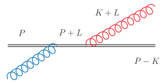
Figure 5.5: One of the extra diagrams that appear once the duration of the jet-medium interaction is comparable to the gluon formation time. The blob represents a resummed Hard Thermal Loop: the $L$ gluon is thus a time-like plasmon. Diagrams corresponding to the other processes of Fig. 5.1, as well as the plasmon emission/gluon absorption crossings are not shown.

Let us write

$$\delta\mathcal{C}(k_{\perp})_{\mathrm{semi}}=\frac{g^{2}C_{R}}{\pi k_{\perp}^{4}}\int\frac{dk^{+}}{k^{+}}\int dl^{-}\delta\left(l^{-}-\frac{k_{\perp}^{2}}{2k^{+}}\right)(1+n_{\text{B}}(k^{+}))\hat{q}\left(\rho_{\perp};l^{-}\right)$$ (5.36)

with $\hat{q}(\rho_{\perp};l^{-})$ is a modified (adjoint) $\hat{q}$ [283, 294] that also accounts for the $l^{-}$-dependence, i.e.

$$\hat{q}(\rho_{\perp};l^{-})=g^{2}C_{A}T\int^{\rho_{\perp}}\frac{d^{2}l_{\perp}}{(2\pi)^{2}}\left[\frac{m_{D}^{2}l_{\perp}^{2}}{(l_{\perp}^{2}+l^{-2})(l_{\perp}^{2}+l^{-2}+m_{D}^{2})}+2\frac{l^{-2}}{l_{\perp}^{2}+l^{-2}}\right].$$ (5.37)

As is shown in detail in App. C.2, the second term appears in the LO computation of the hard contribution to $\hat{q}(\mu_{\perp})$. It’s presence here is perhaps unsurprising; the computation [174] also considers elastic $2\leftrightarrow 2$ scatterings exchanging $k_{\perp}\gg gT$. As that calculation treats this gluon with bare propagators, it does not properly account for its soft dynamics, as encoded by HTL resummation. Hence, the semi-collinear limit of [174] should be subtracted, to avoid double counting it. We are then left with

$$\hat{q}(\rho_{\perp};l^{-})_{\text{subtr}}\equiv\hat{q}(\rho_{\perp};l^{-})-\hat{q}(\rho_{\perp};l^{-})_{\text{\cite[cite]{[\@@bibref{Number}{Arnold:2008vd}{}{}]}}}=g^{2}C_{A}T\int^{\rho_{\perp}}\frac{d^{2}l_{\perp}}{(2\pi)^{2}}\frac{m_{D}^{2}l_{\perp}^{2}}{(l_{\perp}^{2}+l^{-2})(l_{\perp}^{2}+l^{-2}+m_{D}^{2})}.$$ (5.38)

Doing the $l_{\perp}$ integration, assuming that $\rho_{\perp}\ll k_{\perp}\ll\mu_{\perp}$, while at the same time taking $\rho_{\perp}\gg l^{-},\,m_{D}$ yields

$$\hat{q}(\rho_{\perp};l^{-})_{\text{subtr}}=\alpha_{s}C_{A}T\bigg{\{}\underbrace{m_{D}^{2}\ln\left(\frac{\rho_{\perp}^{2}}{m_{D}^{2}}\right)}_{\mathrm{HO}}\,-\underbrace{l^{-2}\ln\left(1+\frac{m_{D}^{2}}{l^{-2}}\right)-m_{D}^{2}\ln\left(1+\frac{l^{-2}}{m_{D}^{2}}\right)}_{l^{-}\,\text{-- dependent}}\bigg{\}}.$$ (5.39)

5.4.1 HOA Contribution to Strict Single Scattering

Let us for the moment only concentrate on the first term. The UV logarithmic divergence, characterised by $\rho_{\perp}$ signals the fact that there lies another region of phase space bordering this one that could also give rise to double logarithmic corrections to $\delta\hat{q}(\mu_{\perp})$. We will come back to this issue. Applying the HOA to the first term above, we get

$$\hat{q}_{0}(\rho_{\perp})=\alpha_{s}C_{A}Tm_{D}^{2}\ln\left(\frac{\rho_{\perp}^{2}}{m_{D}^{2}}\right)\to\hat{q}_{0},$$ (5.40)

where we have inferred the value of $\hat{q}_{0}$ from the single-scattering condition, $\rho_{\perp}\ll\mu_{\perp}$. This approximation is what has been done to arrive at Eq. (5.14). To get the double logarithmic correction, we then only need to do the $k^{+}$ and $k_{\perp}$ integrals. As was done in Sec. 5.2, we instead do the integration in terms of the formation time, $\tau$

$$\delta\hat{q}_{\text{semi}}^{\text{HO}}(\mu_{\perp})=\frac{\alpha_{s}C_{R}}{\pi}\hat{q}_{0}\int_{k^{+}_{\text{IR}}}^{\mu_{\perp}^{2}\tau_{\text{int}}}\frac{dk^{+}}{k^{+}}\left(1+2n_{\text{B}}\left(k^{+}\right)\right)\int_{k^{+}/\mu_{\perp}^{2}}^{\tau_{\text{int}}}\frac{d\tau}{\tau}$$ (5.41)

The integration limits match those that come from integrating over regions $3$ and $4$ of Fig. 5.4. The integration here can be dealt with in exactly the same way as for Eq. (5.20). The result reads

$$\delta\hat{q}_{\mathrm{semi}}^{\text{HO}}(\mu_{\perp}) =\frac{\alpha_{s}C_{R}}{2\pi}\hat{q}_{0}\bigg{[}\frac{4T\ln\left(\frac{\mu_{\perp}^{2}\tau_{\text{int}}}{k^{+}_{\text{IR}}e}\right)}{k^{+}_{\text{IR}}}+\left(\ln^{2}\left(\frac{\mu_{\perp}^{2}\tau_{\text{int}}}{\omega_{T}}\right)-2\gamma_{1}+\frac{\pi^{2}}{4}-\gamma_{E}^{2}\right)\bigg{]}$$

$$+\mathcal{O}\left(k^{+}_{\text{IR}},e^{-\mu_{\perp}\tau_{\text{int}}^{2}/T}\right),$$ (5.42)

where $\gamma_{n}$ is the nth Stieltjes constant. The terms above depending on the IR cutoff, $k^{+}_{\text{IR}}$ indeed suggest sensitivity to the region giving rise to classical corrections [11]. We will elaborate on this further in Sec. 5.8. For completeness, we specify the double logarithmic contribution

$$\delta\hat{q}_{\mathrm{semi\,dlog}}^{\text{HO}}(\mu_{\perp})=\frac{\alpha_{s}C_{R}}{2\pi}\hat{q}_{0}\ln^{2}\frac{\mu_{\perp}^{2}\tau_{\text{int}}}{\omega_{T}}$$ (5.43)

We now add this result to that from in the previous section, Eq. (5.27), the double logarithmic contribution coming from integrating over the region for which $\tau\geq\tau_{\text{int}}$

$$\delta\hat{q}(\mu_{\perp})_{\text{dlog}}=\delta\hat{q}^{\text{few}}_{\text{dlog}}(\mu_{\perp})+\delta\hat{q}_{\mathrm{semi\,dlog}}^{\text{HO}}(\mu_{\perp})=\frac{\alpha_{s}C_{R}}{4\pi}\hat{q}_{0}\ln^{2}\frac{\mu_{\perp}^{4}}{\hat{q}_{0}\omega_{T}}.$$ (5.44)

Upon adding the two contributions together, it is reassuring to observe the disappearance of the intermediate cutoff, $\tau_{\text{int}}$. Moreover, with respect to Eq. (5.17), the IR regulator $\tau_{\text{min}}$ has been replaced with the thermal scale, $\omega_{T}$. This is one of the main results of this thesis; by carefully including the contribution from the thermal scale, we have bypassed many of the issues associated with $\tau_{\text{min}}$, which were highlighted in Sec. 5.3. As we will demonstrate in the next section, Eq. (5.44) turns out to be the dominant contribution to overall double logarithmic correction to $\hat{q}(\mu_{\perp})$.

It is interesting to note that the correction above corresponds (up to the prefactor of $\alpha_{s}C_{R}\hat{q}_{0}/\pi$) to the area of the sum of the “1” and “3” regions from Fig. 5.4. This observation that neither region “2” nor “4 ”contribute makes transparent the fact that, up to double-logarithmic accuracy, the effect of a populated medium can be understood as cutting off the phase space with a vertical, $k^{+}>\omega_{T}\sim T$ line instead of a horizontal $\tau>\tau_{\text{min}}$ line.

Why does the thermal scale have such an effect? To start, we note that for $k^{+}\ll T$

$$2n_{\text{B}}(k^{+})\approx\frac{2T}{k^{+}}-1.$$ (5.45)

Looking to Eq. (5.41), we note that in this limit, the part of the $k^{+}$ integrand giving rise to the logarithmic enhancement will be washed away; the vacuum part – $1$ – cancels against the first quantum correction coming from the expanded $n_{\text{B}}(k^{+})$. This is exactly what is exhibited in Eq. (5.4.1), where $k_{\text{IR}}^{+}$ only appears in the power law term.

5.4.2 $l^{-}$ – Dependent Contrbution to Strict Single Scattering

We now turn to the calculation of the $l^{-}$ – dependent terms in Eq. (5.39). As we will see, this $l^{-}$ dependence renders the integration a little more challenging. Before beginning its evaluation, we use the delta function in Eq. (5.36) to rewrite everything in terms of the formation time, i.e $\tau=k^{+}/k_{\perp}^{2}=1/(2l^{-})$. The starting point is

$$\mathcal{I}(\mu_{\perp})\equiv\int_{k^{+}_{\text{IR}}}^{\mu_{\perp}^{2}\tau_{\text{int}}}\frac{dk^{+}}{k^{+}}\left(\frac{1}{2}+n_{\text{B}}(k^{+})\right)\int_{k^{+}/\mu_{\perp}^{2}}^{\tau_{\text{int}}}\frac{d\tau}{\tau}\left[-\frac{1}{4\tau^{2}}\ln\left(1+4m_{D}^{2}\tau^{2}\right)-m_{D}^{2}\ln\left(1+\frac{1}{4m_{D}^{2}\tau^{2}}\right)\right].$$ (5.46)

The $\tau$ integration yields

$$\mathcal{I}(\mu_{\perp})=\int_{k^{+}_{\text{IR}}}^{\mu_{\perp}^{2}\tau_{\text{int}}}\frac{dk^{+}}{k^{+}}\left(\frac{1}{2}+n_{\text{B}}(k^{+})\right)\bigg{[} \frac{m_{D}^{2}}{2}\mathrm{Li}_{2}\left(-\frac{\mu_{\perp}^{4}}{4k^{+2}m_{D}^{2}}\right)-\frac{m_{D}^{2}}{2}\ln\left(1+\frac{\mu_{\perp}^{4}}{4k^{+2}m_{D}^{2}}\right)$$

$$-\frac{\mu_{\perp}^{4}}{8k^{+2}}\ln\left(1+\frac{4k^{+2}m_{D}^{2}}{\mu_{\perp}^{4}}\right)+\mathcal{O}\left(\frac{1}{\tau_{\text{int}}^{2}}\right)\bigg{]},$$ (5.47)

where $\mathrm{Li}_{2}$ is the dilogarithm and we have expanded for $m_{D}\tau_{\text{int}}\gg 1$, recalling that $1/gT\ll\tau_{\text{int}}\ll 1/g^{2}T$. The vacuum ($1/2$) part needs to be integrated as is, without further expansions: while close to the IR boundary we could exploit that $\mu_{\perp}^{2}/(2k^{+}m_{D})\gg 1$, that would not be true close to the UV boundary, where instead $\mu_{\perp}^{2}/(2k^{+}m_{D})\ll 1$. The integral is however not problematic and yields

$$\mathcal{I}_{\mathrm{vac}}(\mu_{\perp})= -\frac{1}{6}m_{D}^{2}\bigg{[}\ln^{3}\left(\frac{\mu_{\perp}^{2}}{2k^{+}_{\text{IR}}m_{D}}\right)+\frac{3}{2}\ln^{2}\left(\frac{\mu_{\perp}^{2}}{2k^{+}_{\text{IR}}m_{D}}\right)+\frac{1}{4}\left(6+\pi^{2}\right)\ln\left(\frac{\mu_{\perp}^{2}}{2k^{+}_{\text{IR}}m_{D}}\right)+\frac{1}{8}\left(6+\pi^{2}\right)\bigg{]}$$

$$+\mathcal{O}\left(\frac{1}{\tau_{\text{int}}^{2}},(k^{+}_{\text{IR}})^{2}\right),$$ (5.48)

where we have again expanded in the cutoffs. For the thermal part, we can on the other hand expand for $\mu_{\perp}^{2}/(2k^{+}m_{D})\gg 1$, as the effective UV cutoff introduced by Boltzmann suppression makes the region where $\mu_{\perp}^{2}/(2k^{+}m_{D})\lesssim 1$ exponentially suppressed. Hence

$$\mathcal{I}_{T}(\mu_{\perp})=-m_{D}^{2}\int_{k^{+}_{\text{IR}}}^{\infty}\frac{dk^{+}}{k^{+}}n_{\text{B}}(k^{+})\bigg{[} \ln^{2}\frac{\mu_{\perp}^{2}}{2k^{+}m_{D}}+\ln\frac{\mu_{\perp}^{2}}{2k^{+}m_{D}}+\frac{1}{2}\left(1+\frac{\pi^{2}}{6}\right)\bigg{]}+\ldots,$$ (5.49)

where the dots stand for higher-order terms in the expansions in the cutoffs and for the exponentially suppressed term arising from approximating the UV cutoff to infinity. This integral can be done with Eqs. (5.21), (5.24) and

$$\int_{0}^{\infty}\frac{dk^{+}}{k^{+}}k^{+\epsilon}n_{\text{B}}(k^{+})\ln^{2}\frac{k^{+}}{T}=T^{\epsilon}\Gamma(\epsilon)\left[\zeta^{\prime\prime}(\epsilon)+2\psi(\epsilon)\zeta^{\prime}(\epsilon)+\zeta(\epsilon)\left(\psi(\epsilon)^{2}+\psi^{(1)}(\epsilon)\right)\right],$$ (5.50)

where $\psi^{(1)}$ is the polygamma function of order 1. Using these three integrals we find

$$\mathcal{I}_{T}(\mu_{\perp})= -\frac{m_{D}^{2}T\left(\ln^{2}\left(\frac{\mu_{\perp}^{2}}{2k^{+}_{\text{IR}}m_{D}}\right)-\ln\left(\frac{\mu_{\perp}^{2}}{2k^{+}_{\text{IR}}m_{D}}\right)+\frac{\pi^{2}}{12}+\frac{3}{2}\right)}{k^{+}_{\text{IR}}}$$

$$+\frac{m_{D}^{2}}{6}\bigg{\{}\ln^{3}\left(\frac{\mu_{\perp}^{2}}{2k^{+}_{\text{IR}}m_{D}}\right)-\ln^{3}\left(\frac{\mu_{\perp}^{2}}{2m_{D}\omega_{T}}\right)+\frac{3}{2}\ln^{2}\left(\frac{\mu_{\perp}^{2}}{2k^{+}_{\text{IR}}m_{D}}\right)-\frac{3}{2}\ln^{2}\left(\frac{\mu_{\perp}^{2}}{2m_{D}\omega_{T}}\right)$$

$$+\frac{1}{4}\left(6+\pi^{2}\right)\ln\left(\frac{\mu_{\perp}^{2}}{2k^{+}_{\text{IR}}m_{D}}\right)+\ln\left(\frac{\mu_{\perp}^{2}}{2m_{D}\omega_{T}}\right)\left[6\gamma_{1}-\pi^{2}+3\gamma_{E}^{2}-\frac{3}{2}\right]$$

$$-6\gamma_{E}\gamma_{1}-3\left(-\gamma_{1}+\gamma_{2}+\frac{\pi^{2}}{8}\right)+\frac{1}{2}(3-4\gamma_{E})\gamma_{E}^{2}\bigg{\}}+\ldots\,.$$ (5.51)

Upon summing Eqs. (5.48) and (5.51) we see that all logarithmic dependence on $k^{+}_{\text{IR}}$ vanishes, yielding

$$\mathcal{I}(\mu_{\perp})= -\frac{m_{D}^{2}T\left(\ln^{2}\left(\frac{\mu_{\perp}^{2}}{2k^{+}_{\text{IR}}m_{D}}\right)-\ln\left(\frac{\mu_{\perp}^{2}}{2k^{+}_{\text{IR}}m_{D}}\right)+\frac{\pi^{2}}{12}+\frac{3}{2}\right)}{k^{+}_{\text{IR}}}$$

$$+\frac{m_{D}^{2}}{6}\bigg{\{}-\ln^{3}\left(\frac{\mu_{\perp}^{2}}{2m_{D}\omega_{T}}\right)-\frac{3}{2}\ln^{2}\left(\frac{\mu_{\perp}^{2}}{2m_{D}\omega_{T}}\right)+\ln\left(\frac{\mu_{\perp}^{2}}{2m_{D}\omega_{T}}\right)\left[6\gamma_{1}-\pi^{2}+3\gamma_{E}^{2}-\frac{3}{2}\right]$$

$$-6\gamma_{E}\gamma_{1}-3\left(-\gamma_{1}+\gamma_{2}\right)+\frac{1}{2}(3-4\gamma_{E})\gamma_{E}^{2}-\frac{1}{4}\left(3+2\pi^{2}\right)\bigg{\}}+\ldots\,.$$ (5.52)

Upon reinstating the proper prefactor we have

$$\delta\hat{q}_{\mathrm{semi}}^{l^{-}-\mathrm{dep}}(\mu_{\perp})=\frac{2\alpha_{s}^{2}C_{R}C_{A}T}{\pi}\mathcal{I}(\mu_{\perp}),$$ (5.53)

so that

$$\delta\hat{q}_{\text{semi dlog}}^{l^{-}-\mathrm{dep}}(\mu_{\perp})=-\frac{\alpha_{s}^{2}C_{R}C_{A}Tm_{D}^{2}}{3\pi}\ln^{3}\frac{e^{1/2}\mu_{\perp}^{2}}{2\omega_{T}m_{D}}.$$ (5.54)

Let us compare this result to Eq. (5.44). Reinstating the Coulomb logarithm in the latter, it becomes, up to its overall prefactor,

$$\delta\hat{q}_{\mathrm{semi\,dlog}}^{\text{HO}}(\mu_{\perp})\propto\ln\frac{\rho_{\perp}^{2}}{m_{D}^{2}}\ln^{2}\frac{\mu_{\perp}^{2}}{\sqrt{\hat{q}_{0}\omega_{T}}}.$$ (5.55)

Eq. (5.54) in parametrically smaller compared to $\delta\hat{q}_{\mathrm{semi\,dlog}}^{\text{HO}}(\mu_{\perp})$. This can be seen by noting that $\mu_{\perp}^{2}/\sqrt{\hat{q}_{0}\omega_{T}}$ is larger by $1/g$ than $\mu_{\perp}^{2}/(m_{D}\omega_{T})$, which is instead comparable to $\rho_{\perp}^{2}/m_{D}^{2}$, since $\rho_{\perp}\ll\mu_{\perp}$. We thus emphasise that effects analysed in the semi-collinear evaluation, such as the relaxation of the instantaneous approximation are not relevant at double-logarithmic accuracy in the HOA.

5.5 Extension to $\mu_{\perp}>T$

Up until this point, we have taken $T\gg\mu_{\perp}\gg\sqrt{g}T$, the first range where double-logarithm corrections appear. We now move on to consider what happens if $\mu_{\perp}\gg T$ in terms of the structure of the relevant portion of phase space.

If we start from Fig. 5.4 and proceed to increase $\mu_{\perp}$, line $(a)$ gets shifted to the right, making the original $(a)-(b)-(c)$ triangle larger. As we argued previously, once $\mu_{\perp}>\sqrt{\omega_{T}/\tau_{\text{min}}}\sim T$ the vertical $k^{+}=\omega_{T}$ line intersects lines $(b)$ and $(c)$ rather than $(b)$ and $(a)$. Hence, nothing would change for the part of the evaluation for $\tau>\tau_{\text{int}}$, as given by Eq. (5.27). On the other hand, the evaluation of the strict single scattering regime, for $\tau<\tau_{\text{int}}$, needs to be amended to account for this. It must also incorporate that for $\mu_{\perp}\gtrsim T$ we are including strict single scatterings where $l_{\perp}$ is approaching or possibly exceeding the $T$ scale. In principle, one would thus need to account for the fact that the coefficient of the leading-log (harmonic oscillator) $\hat{q}_{0}$ is not constant. As shown in [174] and summarized in Sec. 3.4, $\hat{q}_{0}(\rho\ll T)$ and $\hat{q}_{0}(\rho\gg T)$ differ at leading-log by 15% for $N_{f}=3$ and $N_{c}=3$, so in a first approximation we may neglect this effect. We leave a more precise evaluation of semi-collinear processes in this region to future work.

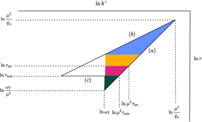
Figure 5.6: Structure of phase space once the cutoff on $\mu_{\perp}$ is allowed to increase to values much larger than the temperature. Notably, region “6” in dark green emerges. It cannot be well described by our setup due to the associated small formation time.

Under this approximation, we can simply extend Eq. (5.44) to the present case. This would however include the dark green triangle “6” in Fig. 5.6, which lies under the $\tau=\tau_{\text{min}}$ line. It is not clear whether this sharp line needs to be included, and only an evaluation like the one we show in detail in the previous section, but extended to larger $\mu_{\perp}$ can address the effect of the relaxation of the instantaneous approximation in this setting. The expectation from the previous $\mu_{\perp}<T$ results is that this effect should be subleading. We however choose to proceed conservatively here and subtract that slice from our result. Moreover, parts of this triangle lie below the $\tau k^{+}=1$ line, further motivating its subtraction. In our double-logarithmic approximation, this corresponds again, for the reasons explained at the end of Sec. 5.4.1, to subtracting off the area of the dark green triangle. This leads to

$$\delta\hat{q}(\mu_{\perp}\gg T)_{\mathrm{dlog}} =\frac{\alpha_{s}C_{R}}{2\pi}\hat{q}_{0}(\rho_{\perp}\ll\mu_{\perp})\left[\frac{1}{2}\ln^{2}\left(\frac{\mu^{4}}{\hat{q}_{0}\omega_{T}}\right)-\ln^{2}\left(\frac{\mu_{\perp}^{2}\tau_{\text{min}}}{\omega_{T}}\right)\right]$$

$$=\frac{\alpha_{s}C_{R}}{2\pi}\hat{q}_{0}(\rho_{\perp}\ll\mu_{\perp})\left[\ln^{2}\left(\frac{\mu^{2}}{\hat{q}_{0}\tau_{\text{min}}}\right)-\frac{1}{2}\ln^{2}\left(\frac{\omega_{T}}{\hat{q}_{0}\tau_{\text{min}}^{2}}\right)\right].$$ (5.56)

Unsurprisingly, the subtraction of the “6” triangle from the “1+3+6” triangle on the first line is equal to that of the unshaded “2+5” triangle from the original $(a)-(b)-(c)$ triangle on the second line. This implies that, for $\mu_{\perp}>T$, our result is closer to the original one of [1].

This can be better appreciated by noting that the vertical line at $k^{+}=\mu_{\perp}^{2}\tau_{\text{min}}$ cuts the $(a)-(b)-(c)$ triangle into two triangles of equal area. Hence, for $\omega_{T}>\mu_{\perp}^{2}\tau_{\text{min}}$, i.e. $\mu_{\perp}\lesssim T$ our result (5.44) is less than half of the original double logarithm (5.17), whereas for $\mu_{\perp}>\sqrt{\omega_{T}/\tau_{\text{min}}}$ our result (5.56) is more than half of it.

5.6 Analysis of Neighbouring Regions

In the previous section, we showed that the dominant contribution to double logarithmic corrections to $\hat{q}(\mu_{\perp})$ in a weakly coupled QGP are given by the result Eq. (5.44). On the way to arriving at this result, we took the HOA; the dependence on $\rho_{\perp}$, the UV cutoff for $l_{\perp}$ in the first term of Eq. (5.39) signals sensitivity to a neighbouring region with larger $l_{\perp}$, which could also potentially possess a double logarithmic enhancement. In this section, we explore a couple of adjacent regions of phase space and comment on whether or not they are relevant with respect to our ultimate pursuit.

5.6.1 $l_{\perp}\sim\sqrt{g}T,\,l^{+}\sim l^{-}\sim gT$

Since we now have $L^{2}\gg m_{D}^{2}$, we can start by expanding $G_{rr}^{--}(L)$, which will inevitably appear in our evaluation

$$G_{rr}^{--}(L) =\Big{(}\frac{1}{2}+n_{\text{B}}(l^{0})\Big{)}\Big{(}\rho_{\text{B}}^{L}(l)+\frac{l_{\perp}^{2}}{l^{2}}\rho_{\text{B}}^{T}(l)\Big{)}$$

$$\approx\frac{T}{l^{0}}\Big{(}\rho_{\text{B}}^{L}(l)+\frac{l_{\perp}^{2}}{l^{2}}\rho_{\text{B}}^{T}(l)\Big{)}.$$

The expansion ($l^{0}\ll T$) is also valid for the scaling presented in the previous section. However, looking in more detail at the spectral function, we see that

$$\rho^{L}_{\text{B}}(l) =G_{R}^{L}(l)-G_{A}^{L}(l)$$

$$=\frac{i}{l^{2}+\Pi_{R}^{L}(l)}-\frac{i}{l^{2}+\Pi_{A}^{L}(l)}$$

$$\approx\frac{i}{l^{2}}-\frac{i\Pi_{R}^{L}(l)}{l^{4}}-\frac{i}{l^{2}}+\frac{i\Pi_{A}^{L}(l)}{l^{4}}$$

where the causal HTL propagators have been defined in Eqs. (4.72),  (LABEL:htltrans). Let us now further unpack the causal self energies

$$\Pi_{R/A}^{L}(l) =m_{D}^{2}\Big{(}1-\frac{l^{0}\pm i\varepsilon}{2l}\log\frac{l^{0}+l\pm i\varepsilon}{l^{0}-l\pm i\varepsilon}\Big{)}$$

$$=m_{D}^{2}\Big{(}1-\frac{l^{0}\pm i\varepsilon}{2l}\Big{(}\log|\frac{l^{0}+l}{l^{0}-l}\Big{|}+i\arctan\frac{\mp 2l\varepsilon}{L^{2}}\Big{)}\Big{)}$$

$$=m_{D}^{2}\Big{(}1-\frac{l^{0}}{2l}\Big{(}\log|\frac{l^{0}+l}{l^{0}-l}\Big{|}\mp i\pi\Theta(-L^{2})\Big{)}\Big{)}$$ (5.57)

where in going to the last line we have taken $\varepsilon\to 0$. When taking the difference of the retarded and advanced self energies, only the imaginary term survives and so

$$\rho^{L}_{\text{B}}(l) =\frac{m_{D}^{2}\pi l^{0}}{l^{5}}\Theta(-L^{2})$$

$$\approx\frac{m_{D}^{2}\pi l^{0}}{l_{\perp}^{5}}$$ (5.58)

where we have used that $L$ is spacelike in going to the second line. Similarly, the transverse spectral function can be computed to give

$$\rho_{\text{B}}^{T}(l) =\frac{m_{D}^{2}\pi l^{0}}{2lL^{4}}\Big{(}1-\frac{{l^{0}}^{2}}{l^{2}}\Big{)}\Theta(-L^{2})$$ (5.59)

$$\approx\frac{m_{D}^{2}\pi l^{0}}{2l_{\perp}^{5}}$$ (5.60)

Next, we can go back to Sec. 5.1, add up the contributions from the three diagrams and expand in $g$ in the usual coft scaling, $K\sim(T,gT,\sqrt{g}T)$, while at the same time taking into account our new scaling for $L$

$$\delta\mathcal{C}(k_{\perp})_{l_{\perp}\sim\sqrt{g}T} =g^{4}C_{R}C_{A}\int\frac{dk^{+}}{2\pi}\int\frac{dl^{+}d^{2}l_{\perp}}{(2\pi)^{3}}\frac{1+n_{\text{B}}(k^{+})}{2k^{+}}\frac{4l_{\perp}^{2}}{k_{\perp}^{2}(\mathbf{k}+\mathbf{l})^{2}}G^{--}_{rr}(-L)$$

$$=g^{4}C_{R}C_{A}\int\frac{dk^{+}}{2\pi}\int\frac{dl^{+}d^{2}l_{\perp}}{(2\pi)^{3}}\frac{1+n_{\text{B}}(k^{+})}{2k^{+}}\frac{4l_{\perp}^{2}}{k_{\perp}^{2}(\mathbf{k}+\mathbf{l})^{2}}\frac{3Tm_{D}^{2}}{2l_{\perp}^{5}}.$$ (5.61)

The integrand is independent of $l^{+}$ and so after the integration has been done, the result will be proportional to a power of the cutoff on $l^{+}$. As is always the case when one is computing integrals using the method of regions, this cutoff term will be cancelled by the integration done in some other adjacent region. However, we know that in the $L\sim(gT,gT,gT)$ scaling, adopted in the previous section, there are no terms that depend on the $l^{+}$ cutoff. We can therefore conclude that this region is not adjacent to that region, implying that we need not concern ourselves with it. We have checked that something similar happens with the scaling $(l^{+},l^{-},l_{\perp})\sim(\sqrt{g}T,gT,gT)$ and so we discard this region as well.

5.6.2 $l_{\perp}\sim l^{+}\sim\sqrt{g}T,l^{-}\sim gT$

We proceed similarly to the last section by first calculating the expanded spectral functions with this new scaling. The spectral functions read

$$\rho^{L}_{\text{B}}(L) =\frac{m_{D}^{2}\pi l^{0}}{l^{5}}\Theta(-L^{2})$$

$$\approx\frac{m_{D}^{2}\pi l^{+}}{({l^{+}}^{2}+l_{\perp}^{2})^{\frac{5}{2}}}$$ (5.62)

and

$$\rho_{\text{B}}^{T}(L) =\frac{m_{D}^{2}\pi l^{0}}{2lL^{4}}\Big{(}1-\frac{{l^{0}}^{2}}{l^{2}}\Big{)}\Theta(l^{2}-{l^{0}}^{2})$$

$$\approx\frac{m_{D}^{2}\pi l^{+}}{2l_{\perp}^{2}({l^{+}}^{2}+l_{\perp}^{2})^{\frac{3}{2}}}.$$ (5.63)

When using these to compute the scattering kernel, we see that this time, the integrand does depend on $l^{+}$

$$\delta\mathcal{C}(k_{\perp})_{l^{+}\sim l_{\perp}\sim\sqrt{g}T} =g^{4}C_{R}C_{A}\int\frac{dk^{+}}{2\pi}\int\frac{dl^{+}d^{2}l_{\perp}}{(2\pi)^{3}}\frac{1+n_{\text{B}}(k^{+})}{2k^{+}}\frac{4l_{\perp}^{2}}{k_{\perp}^{2}(\mathbf{k}+\mathbf{l})^{2}}G^{--}_{rr}(-L)$$

$$=g^{4}C_{R}C_{A}\int\frac{dk^{+}}{2\pi}\int\frac{dl^{+}d^{2}l_{\perp}}{(2\pi)^{3}}\frac{1+n_{\text{B}}(k^{+})}{2k^{+}}\frac{4l_{\perp}^{2}}{k_{\perp}^{2}(\mathbf{k}+\mathbf{l})^{2}}\frac{3Tm_{D}^{2}\pi}{2({l^{+}}^{2}+l_{\perp}^{2})^{\frac{5}{2}}}$$

$$=2g^{4}C_{R}C_{A}\int\frac{dk^{+}}{2\pi}\int\frac{d^{2}l_{\perp}}{(2\pi)^{2}}\frac{1+n_{\text{B}}(k^{+})}{k^{+}}\frac{Tm_{D}^{2}}{k_{\perp}^{2}(\mathbf{k}+\mathbf{l})^{2}l_{\perp}^{2}}.$$ (5.64)

It is not difficult to check that if we expand the expression above for $k_{\perp}\gg l_{\perp}$, we recover Eq. (5.34), with the $l_{\perp}\gg l^{-}\sim m_{D}$ limit taken there. The fact that these two expressions agree in these limits implies that share a common boundary and are thus adjacent.

The $d^{2}l_{\perp}$ integration would, in this scaling run over the $\mathbf{k}+\mathbf{l}\approx 0$ range, corresponding to a longer-lived bremsstrahlung. Given this longer lifetime, we can expect multiple soft scatterings at a rate of $g^{2}T$ to occur, in addition to a single, harder scattering. Addressing this region properly would thus consist of dealing with LPM resummation beyond the HOA. It is for this reason that we have been forced to adopt the HOA and in doing so, are not able to compute the double logarithmic contribution coming from this region. We discuss a pathway to dealing with this issue in the next section.

5.7 Momentum Broadening Beyond the HOA

To briefly recap, up until this point, we have managed to compute double-logarithmic corrections to $\hat{q}(\mu_{\perp})$, with the dominant corrections coming from Eq. (5.44). In arriving at that expression, we observed sensitivity to a neighbouring region (studied in Sec. 5.6.2) that allows for both single and multiple scattering, which requires a more involved treatment. We postponed dealing with this region by taking the HOA, inferring the coefficient of $\hat{q}_{0}$ from the single-scattering consideration $\mu_{\perp}\gg\rho_{\perp}$. In addition, we have had to impose by hand the boundary $(b)$, which is intended to partition the single and multiple scattering regimes. This is in contrast to the boundary separating the double-logarithmic phase space from its classical counterpart, which, as we will demonstrate, is clearly cut off by the scale $\omega_{\text{T}}$. In this section, we present a way to proceed beyond these two hurdles, to self-consistently determine $\delta\hat{q}(\mu_{\perp})$.

To this end, we will derive, starting from the formalism of [1, 220], an LPM resummation equation that is not restricted to the HOA. By numerically solving that equation and performing the integrations over the two logarithmic variables $k^{+}$ and $\tau$ (or equivalently $k^{+}$ and $k_{\perp}$) one would then see the emergence of multiple scatterings cutting off the double-log and thus be able to determine how good of an approximation line $(b)$ is. Let us then start from Eqs. (6), (7), (11) and (12) in [1] (see also (55)), which construct a framework for resumming multiple interactions in the HOA and in the large-$N_{c}$ limit. Combining (11) and (12) yields, in the notation of [1]

$$S(x_{\perp})=-\alpha_{s}C_{R}\mathrm{Re} \int\frac{dk^{+}}{{k^{+}}^{3}}\int_{0}^{L_{M}}dz_{2}\int_{0}^{z_{2}}dz_{1}\nabla_{\mathbf{b}_{2}}\cdot\nabla_{\mathbf{b}_{1}}$$

$$\times\bigg{[}e^{-\hat{q}_{0\,R}x_{\perp}^{2}(L_{M}-z_{2}+z_{1})/4}G_{\text{HOA}}(\mathbf{b}_{2},z_{2};\mathbf{b}_{1},z_{1})-\mathrm{vac}\bigg{]}\bigg{|}^{\mathbf{b}_{2}=\mathbf{x}}_{\mathbf{b}_{2}=0}\bigg{|}^{\mathbf{b}_{1}=\mathbf{x}}_{\mathbf{b}_{1}=0},$$ (5.65)

where we have already undone the large-$N_{c}$ approximation by replacing $N_{c}/2$, the original large-$N_{c}$ limit of $C_{F}$, with $C_{R}$. $\hat{q}_{0\,R}$, with $R=F,G$ denotes the specific partonic broadening coefficients for a quark or gluon source. The $dk^{+}$ frequency integration is understood over the positive frequencies of the radiated gluon. The propagator $G_{\text{HOA}}$ is the Green’s function of the following Schrödinger equation (see (55) there)

$$\bigg{\{}i\partial_{z}+\frac{\nabla^{2}_{\mathbf{b}}}{2k^{+}}+\frac{i}{4}\bigg{[}\hat{q}_{0R}x_{\perp}^{2}+\frac{\hat{q}_{0A}}{2}\big{(}b_{\perp}^{2}+(\mathbf{b}-\mathbf{x})^{2}-x_{\perp}^{2}\big{)}\bigg{]}\bigg{\}}G_{\text{HOA}}(\mathbf{b},z;\mathbf{b}_{1},z_{1})=0,$$ (5.66)

with

$$G_{\text{HOA}}(\mathbf{b},z_{1};\mathbf{b}_{1},z_{1})=\delta^{(2)}(\mathbf{b}-\mathbf{b}_{1}).$$ (5.67)

“vac” denotes the subtraction of the vacuum term $G_{0}$, i.e. the solution of Eq. (5.71) with a vanishing $\hat{q}_{0}$. The double vertical bars at the end of Eq. (5.65) signify that the expression in brackets should be understood as

$$e^{-\frac{\hat{q}_{0\,R}x_{\perp}^{2}}{4}(L_{M}-z_{2}+z_{1})}\bigg{[} G_{\text{HOA}}(\mathbf{x},z_{2};\mathbf{x},z_{1})+G_{\text{HOA}}(0,z_{2};0,z_{1})$$

$$-G_{\text{HOA}}(\mathbf{x},z_{2};0,z_{1})-G_{\text{HOA}}(0,z_{2};\mathbf{x},z_{1})\bigg{]}-\mathrm{vac}.$$ (5.68)

Physically, these four terms can be understood as the two positive, virtual terms, where the gluon is emitted and reabsorbed within the amplitude (both $\mathbf{b}=0$) or conjugate amplitude (both $\mathbf{b}=\mathbf{x}$) minus the real terms, where the gluon is emitted on one side and absorbed on the other side of the cut.

As a first step, we can identify their $S$-matrix element with our $\langle W(x_{\perp})\rangle$. Hence we can equate

$$S(x_{\perp})=\exp[-L_{M}(\mathcal{C}(x_{\perp})+\delta\mathcal{C}(x_{\perp}))]\approx e^{-L_{M}\mathcal{C}(x_{\perp})}(1-L_{M}\delta\mathcal{C}(x_{\perp})).$$ (5.69)

Secondly, Eq. (5.65) is in the harmonic-oscillator approximation, i.e.

$$\mathcal{C}_{R}(x_{\perp})\stackrel{{\scriptstyle{\text{HOA}}}}{{=}}\frac{\hat{q}_{0\,R}}{4}x_{\perp}^{2},$$ (5.70)

We can then undo this approximation so that Eq. (5.66) becomes

$$\bigg{\{}i\partial_{z}+\frac{\nabla^{2}_{\mathbf{b}}-m_{\infty\,g}^{2}}{2k^{+}}+i\bigg{[}\mathcal{C}_{R}(x_{\perp})+\frac{1}{2}\big{(}\mathcal{C}_{A}(b_{\perp})+\mathcal{C}_{A}(|\mathbf{b}-\mathbf{x}|)-\mathcal{C}_{A}(x_{\perp})\big{)}\bigg{]}\bigg{\}}G(\mathbf{b},z;\mathbf{b}_{1},z_{1})=0,$$ (5.71)

where we have also introduced the gluon’s asymptotic mass, with $m_{\infty\,g}^{2}=m_{D}^{2}/2$ . To extract a leading-order determination of radiative correction from this formalism, it should suffice to use, for $\mathcal{C}_{F}(x_{\perp}),\,\mathcal{C}_{A}(x_{\perp})$ the Fourier transform of the smooth kernel provided by Eq. (3.56).

Finally, we can also account for the effect of a populated medium by considering the effects of stimulated emission and absorption, i.e $\int dk^{+}\Theta(k^{+})\to\int dk^{+}(1/2+n_{\text{B}}(k^{+}))$. In a longitudinally uniform medium, $G$ is only a function of $t\equiv z_{2}-z_{1}$ so that we can use our identification (5.69) to obtain, in the large-$L_{M}$ limit

$$\delta\mathcal{C}(x_{\perp})=\alpha_{s}C_{R}\mathrm{Re}\int\frac{dk^{+}}{k^{+3}}\left(\frac{1}{2}+n_{\text{B}}(k^{+})\right)\int_{0}^{L_{M}}dt\,\nabla_{\mathbf{b}_{2}}\cdot\nabla_{\mathbf{b}_{1}}\bigg{[} e^{\mathcal{C}_{R}(x_{\perp})t}G(\mathbf{b}_{2},\mathbf{b}_{1};t)$$

$$-\mathrm{vac}\bigg{]}\bigg{|}^{\mathbf{b}_{2}=\mathbf{x}}_{\mathbf{b}_{2}=0}\bigg{|}^{\mathbf{b}_{1}=\mathbf{x}}_{\mathbf{b}_{1}=0}.$$ (5.72)

We observe that the source-specific part of the scattering kernel in the Hamiltonian (5.71) and the amplification factor $e^{\mathcal{C}_{R}(x_{\perp})t}$ above can be eliminated by noting that if $\tilde{G}(\mathbf{b},\mathbf{b}_{1};t)\equiv e^{\mathcal{C}_{R}(x_{\perp})t}G(\mathbf{b},\mathbf{b}_{1};t)$ is a Green’s function of the operator

$$\bigg{\{}i\partial_{t}+\frac{\nabla^{2}_{\mathbf{b}}-m_{\infty\,g}^{2}}{2k^{+}}+\frac{i}{2}\big{(}\mathcal{C}_{A}(b_{\perp})+\mathcal{C}_{A}(|\mathbf{b}-\mathbf{x}|)-\mathcal{C}_{A}(x_{\perp})\big{)}\bigg{\}}\tilde{G}(\mathbf{b},\mathbf{b}_{1};t)=0,$$ (5.73)

then $G(\mathbf{B},\mathbf{B}_{1};t)$ is a Green’s function of Eq. (5.71). Hence

$$\delta\mathcal{C}(x_{\perp})=\alpha_{s}C_{R}\mathrm{Re}\int\frac{dk^{+}}{k^{+3}}\left(\frac{1}{2}+n_{\text{B}}(k^{+})\right)\int_{0}^{L_{M}}dt\,\nabla_{\mathbf{b}_{2}}\cdot\nabla_{\mathbf{b}_{1}}\bigg{[} \tilde{G}(\mathbf{b}_{2},\mathbf{b}_{1};t)$$

$$-\mathrm{vac}\bigg{]}\bigg{|}^{\mathbf{b}_{2}=\mathbf{x}}_{\mathbf{b}_{2}=0}\bigg{|}^{\mathbf{b}_{1}=\mathbf{x}}_{\mathbf{b}_{1}=0}.$$ (5.74)

This reformulation makes transparent the fact that the Hamiltonian only contains the purely non-abelian $\mathcal{C}_{A}$. That is because before or after both emission vertices, there are only the two source lines for the hard jet parton and one-gluon exchanges between them are resummed into $\exp\big(-\mathcal{C}_{R}(x_{\perp})(L_{M}-t)\big{missing})$. In the time region between the two emission vertices, the hard jet parton and conjugate hard jet parton lines are no longer a color singlet, with corresponding color factor $C_{R}$, but rather an octet, with color factor $C_{R}-C_{A}/2$. This corresponds to the $\mathcal{C}_{R}(x_{\perp})-\mathcal{C}_{A}(x_{\perp})/2$ combination in Eq. (5.71). But we should remove the overall $\exp\big(-\mathcal{C}_{R}(x_{\perp})L_{M}\big{missing})$ damping, which, as per our dictionary (5.69), leads to the outright disappearance of the $\mathcal{C}_{R}(x_{\perp})$ part, corresponding to the fact that those exchanges would happen also in the absence of the radiated gluon. Up to the statistical factors and thermal masses, Eqs. (5.73) and  (5.74) agree with [220].

For a medium that is isotropic in the azimuthal direction, we can use the reflection symmetry $\mathbf{b}\to\mathbf{x}-\mathbf{b}$ of Eq. (5.73) to simplify Eq. (5.74) into

$$\delta\mathcal{C}(x_{\perp})=-2\alpha_{s}C_{R}\mathrm{Re}\int\frac{dk^{+}}{k^{+3}}\left(\frac{1}{2}+n_{\text{B}}(k^{+})\right)\int_{0}^{L_{M}}dt\,\nabla_{\mathbf{b}_{2}}\cdot\nabla_{\mathbf{b}_{1}}\bigg{[} \tilde{G}(\mathbf{b}_{2},\mathbf{b}_{1};t)$$

$$-\mathrm{vac}\bigg{]}\bigg{|}^{\mathbf{b}_{2}=\mathbf{x},\mathbf{b}_{1}=0}_{\mathbf{b}_{2}=0,\mathbf{b}_{1}=0}.$$ (5.75)

Eq. (5.73) is, together with Eq. (5.75), the main result of this section. We anticipate that its solution would allow for a much better understanding of how the double logarithm is cut off by the transition from single to multiple scatterings as a function of the energy $k^{+}$ of the radiated gluon. Furthermore, Eq. (5.73) goes beyond the HOA and would thus allow us to properly deal with the region (discussed in Sec. 5.6.2) where $\mathbf{l}+\mathbf{k}$ become small and in turn develop sensitivity to multiple scatterings. However, Eq. (5.73) is not easy to solve, as it would require generalizing the methods of [159, 198, 299, 14] to the extra dependence on $x_{\perp}$ of $\tilde{G}$. As a first step, one could consider using the improved opacity expansion, already mentioned in Sec. 3.7 to capture the qualitative aspects of the transition from the HO approximation to including rarer harder scatterings.

We shall leave the full or approximate solution of Eq. (5.73) to future work. We continue this section by providing a non-trivial consistency check, namely that the single-scattering term in Eqs. (5.73) and (5.75) agrees with Eq. (5.12). The calculation here proceeds in exactly the same way as for the single-scattering rate, derived in Sec. 3.5. Following the same steps, we arrive at

$$\delta\mathcal{C}(x_{\perp})^{N=1}=2\alpha_{s}C_{R}\int\frac{dk^{+}}{k^{+}} \left(1+2n_{\text{B}}(k^{+})\right)\int_{\mathbf{p}}\int_{\mathbf{l}}\,\mathcal{C}_{A}(l_{\perp})\frac{(1-e^{i\mathbf{x}\cdot\mathbf{p}})(1+e^{i\mathbf{x}\cdot\mathbf{l}})}{p_{\perp}^{2}+m_{\infty\,g}^{2}}$$

$$\times\bigg{[}\frac{p_{\perp}^{2}}{p_{\perp}^{2}+m_{\infty\,g}^{2}}-\frac{\mathbf{p}\cdot(\mathbf{p}+\mathbf{l})}{(\mathbf{p}+\mathbf{l})^{2}+m_{\infty\,g}^{2}}\bigg{]}.$$ (5.76)

We take a moment here to compare the equation above with Eq. (3.66), with the $L_{M}\to\infty$ limit taken there. Even though the latter equation is a radiation splitting rate, we can immediately understand that it resembles the former, which computes corrections to the scattering kernel due to radiative processes. However, the product $(1-e^{i\mathbf{x}\cdot\mathbf{p}})(1+e^{i\mathbf{x}\cdot\mathbf{l}})$ above makes manifest that the above equation includes real, probability-conserving as well as virtual processes in comparison to Eq. (3.66), which only contains real processes. To make contact with Eq. (5.12), we need to extract the real-process contribution, $\delta\mathcal{C}(k_{\perp})^{\mathrm{real}}_{\mathrm{single}}$. This just corresponds to Fourier-transforming $\mathbf{x}$ into $\mathbf{k}$ and only keeping terms proportional to $\exp(i\mathbf{x}\cdot\mathbf{p})$ and $\exp(i\mathbf{x}\cdot(\mathbf{p}+\mathbf{l}))$, yielding

$$\delta\mathcal{C}(k_{\perp})^{\mathrm{real}}_{\mathrm{single}}= 4\alpha_{s}C_{R}\int dk^{+}\frac{\frac{1}{2}+n_{\text{B}}(k^{+})}{k^{+}}\int_{\mathbf{l}}\mathcal{C}_{g}(l_{\perp})\left[\frac{\mathbf{k}}{k_{\perp}^{2}+m_{\infty\,g}^{2}}-\frac{\mathbf{k}+\mathbf{l}}{(\mathbf{k}{+}\mathbf{l})^{2}+m_{\infty\,g}^{2}}\right]^{2},$$ (5.77)

which, in the $m_{\infty\,g}\to 0$ and ($1/2+n_{\text{B}}(k^{+})\to\Theta(k^{+})$) limits agree with Eq. (5.12). In App. C.3 we compute the aforementioned virtual contributions diagrammatically and in doing so, check that they are consistent with Eq. (5.76).

5.8 Connection to the Classical Contribution

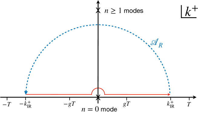
Figure 5.7: The contour discussed in the main text for the evaluation of the retarded part of the soft contribution to $\delta\mathcal{C}(k_{\perp})$. The corresponding advanced part is not shown. The cross at the origin is Matsubara zero mode, hence the deformation of the (red) integration contour there, which gives rise to the Euclidean contribution.

When computing double logarithmic corrections to $\hat{q}(\mu_{\perp})$ in Sec. 5.4, we observed corrections depending on a power law of the IR energy cutoff, $k^{+}_{\text{IR}}$. Power law corrections of this kind will always cancel against those coming from a neighbouring region of phase space and in some sense, can be disregarded. In this instance however, we take advantage of this fact to further clarify how the region of phase space from which the quantum corrections emerge is connected to the region giving rise to the classical corrections. In particular, we set out to show how the first term in Eq. (5.4.1) is also produced (but with an opposite sign) in the calculation of Caron-Huot [11]. We do not show how power law corrections from either Eq. (5.26) or Eq. (5.52) cancel against their classical counterparts.

But how should this work in practice? Well, diagrams such as those in Fig. 5.2 are precisely those evaluated in [11] with $K\sim L\sim gT$. On that side, the calculation should produce a $\sim 1/k^{+}_{\text{IR}}$ term. There, $k^{+}_{\text{IR}}$ is a UV cutoff, which can thus be safely sent to infinity, resulting in the absence of such corrections from [11].

As we have discussed in Sec. 4.3, based on ideas from the same paper, the classical contribution is dominated by the Matsubara zero mode, which can be mapped to EQCD. In terms of doing the $k^{+}$ integration in the 4D theory, this consists of making the replacement $1/2+n_{\text{B}}(k^{+})\to T/k^{+}$ before closing the integration contour, $\mathcal{A}$ at a radius, $k^{+}_{\text{IR}}$ between the zero and first Matsubara modes. This is moreover consistent with our calculation, in the sense that $gT\ll k^{+}_{\text{IR}}\ll T$. Any function that falls to zero faster than $1/k^{+}$ on this arc will only give rise to inverse powers of $k^{+}_{\text{IR}}$, which could be safely neglected in the derivation [11]. The contour of interest is depicted in Fig. 5.7.

Rather than starting from Caron-Huot’s calculation, we instead begin from around Eq. (F.49) [294], which provides the NLO calculation of the longitudinal momentum diffusion constant, $\hat{q}_{L}(\mu_{\perp})\equiv\langle q_{z}^{2}\rangle/L_{M}$, also conveniently carried out in Coulomb gauge. To make the connection with its transverse counterpart, one can multiply by $(k_{\perp}/k^{+})^{2}$ under the integral sign. This yields

$$\delta\hat{q}\Big{|}_{\mathrm{soft}}^{\mathrm{arcs}}(\mu_{\perp})\!\! = 2g^{4}C_{R}C_{A}T\!\int_{\mathcal{A}_{R}}\!\frac{dk^{+}}{2\pi}\!\int^{\mu_{\perp}}\!\frac{d^{2}k_{\perp}}{(2\pi)^{2}}\!\int_{L}$$

$$\times\bigg{\{}\frac{k_{\perp}^{2}}{k^{+2}}G^{--}_{rr}(L)\pi\delta(l^{-})\left(\frac{\mathbf{k}}{k_{\perp}^{2}+m_{\infty}^{2}}-\frac{\mathbf{k}+\mathbf{l}}{(\mathbf{k}+\mathbf{l})^{2}+m_{\infty}^{2}}\right)^{2}+\mathcal{O}\left(\frac{1}{k^{+3}}\right)\bigg{\}}+\mathcal{A}_{A}.$$

We can now perform some of the $L$ integrations using the reduction to EQCD discussed in Sec. 4.3, finding

$$\delta\hat{q}\Big{|}_{\mathrm{soft}}^{\mathrm{arcs}}(\mu_{\perp})\!\! = g^{4}C_{R}C_{A}T^{2}\!\int_{\mathcal{A}_{R}}\!\frac{dk^{+}}{2\pi}\!\int^{\mu_{\perp}}\!\frac{d^{2}k_{\perp}}{(2\pi)^{2}}\!\int_{\mathbf{l}}$$

$$\times\bigg{\{}\frac{k_{\perp}^{2}}{k^{+2}}\frac{m_{D}^{2}}{l_{\perp}^{2}(l_{\perp}^{2}+m_{D}^{2})}\left(\frac{\mathbf{k}}{k_{\perp}^{2}+m_{\infty}^{2}}-\frac{\mathbf{k}+\mathbf{l}}{(\mathbf{k}+\mathbf{l})^{2}+m_{\infty}^{2}}\right)^{2}+\mathcal{O}\left(\frac{1}{k^{+3}}\right)\bigg{\}}+\mathcal{A}_{A}.$$

If we take the $l_{\perp},m_{D}\ll k_{\perp}$ approximation, consistently with our treatment across the $k^{+}_{\text{IR}}$ boundary, we find

$$\delta\hat{q}\Big{|}_{\mathrm{soft}}^{\mathrm{arcs}}(\mu_{\perp})\!\! = g^{4}C_{R}C_{A}T^{2}\!\int_{\mathcal{A}_{R}}\!\frac{dk^{+}}{2\pi}\!\int^{\mu_{\perp}}\!\frac{d^{2}k_{\perp}}{(2\pi)^{2}}\!\int_{\mathbf{l}}\frac{1}{k^{+2}k_{\perp}^{2}}\frac{m_{D}^{2}}{l_{\perp}^{2}+m_{D}^{2}}+\mathcal{A}_{A}.$$ (5.80)

We regulate the $l_{\perp}$ integration using the HOA consistently with what we did in Sec. 5.4.1, we find

$$\delta\hat{q}\Big{|}_{\mathrm{soft}}^{\mathrm{arcs\,HO}}(\mu_{\perp})\!\! = g^{2}C_{R}T\hat{q}_{0}\!\int_{\mathcal{A}_{R}}\!\frac{dk^{+}}{2\pi}\!\int^{\mu_{\perp}}\!\frac{d^{2}k_{\perp}}{(2\pi)^{2}}\frac{1}{k^{+2}k_{\perp}^{2}}+\mathcal{A}_{A}.$$ (5.81)

We can then rewrite the $k_{\perp}$ integration as a $\tau$ one, with the same boundaries of Eq. (5.41), i.e.

$$\delta\hat{q}\Big{|}_{\mathrm{soft}}^{\mathrm{arcs\,HO}}(\mu_{\perp})\!\! = g^{2}C_{R}T\hat{q}_{0}\!\int_{\mathcal{A}_{R}}\!\frac{dk^{+}}{2\pi}\!\int_{k^{+}/\mu_{\perp}^{2}}^{\tau_{\text{int}}}\!\frac{d\tau}{4\pi}\frac{1}{k^{+2}\tau}+\mathcal{A}_{A}.$$ (5.82)

The contribution on the arc can be carried out as follows, understanding the arc to be at constant $|k^{+}|=k^{+}_{\text{IR}}$. Changing variables to $k^{+}=k^{+}_{\text{IR}}e^{it}$ then gives

$$\int_{\mathcal{A}_{R}}\!\frac{dk^{+}}{2\pi}\frac{1}{k^{+2}}\ln\left(\frac{\mu_{\perp}^{2}\tau_{\text{int}}}{k^{+}}\right)=\frac{i}{2\pi k^{+}_{\text{IR}}}\int_{\pi}^{0}dte^{-it}\bigg{[}\ln\left(\frac{\mu_{\perp}^{2}\tau_{\text{int}}}{k^{+}_{\text{IR}}}\right)-it\bigg{]}=\frac{-1}{\pi k^{+}_{\text{IR}}}\bigg{[}\ln\left(\frac{\mu_{\perp}^{2}\tau_{\text{int}}}{k^{+}_{\text{IR}}}\right)-1-i\frac{\pi}{2}\bigg{]}.$$ (5.83)

The imaginary part cancels against an opposite one from $\mathcal{C}_{A}$. We then have

$$\delta\hat{q}\Big{|}_{\mathrm{soft}}^{\mathrm{arcs\,HO}}(\mu_{\perp})\!\!= 2\frac{g^{2}C_{R}T^{2}\hat{q}_{0}}{4\pi}\frac{-1}{\pi k^{+}_{\text{IR}}}\bigg{[}\ln\left(\frac{\mu_{\perp}^{2}\tau_{\text{int}}}{k^{+}_{\text{IR}}}\right)-1\bigg{]}$$

$$= -2\frac{\alpha_{s}C_{R}T\hat{q}_{0}}{\pi k^{+}_{\text{IR}}}\bigg{[}\ln\left(\frac{\mu_{\perp}^{2}\tau_{\text{int}}}{k^{+}_{\text{IR}}}\right)-1\bigg{]}.$$ (5.84)

This is precisely opposite to the $T/k^{+}_{\text{IR}}$-proportional part of Eq. (5.4.1), as we set out to show.

We provide a final comment with respect to how the double-logarithmic phase space is cut off. The $k^{+}$ integration is clearly cut off around the scale $\omega_{T}$ because below that scale, there is the cancellation between the vacuum term and the first quantum correction, as was explained explicitly around (…), which renders the $k^{+}$ integrand $\sim 1/{k^{+}}^{2}$. But can one understand how the $\tau$ integration transitions to power law behaviour? Well, we can understand from the calculation above that there is no analogous scale to $\omega_{T}$ since a $1/\tau$ integrand persists for $k^{+}\ll T$. Instead, $\omega_{T}$ cuts off the $\tau$ logarithm in a somewhat subtle way; in approaching the $k^{+}_{\text{IR}}$ vertical line from the right, the $\tau$ integration gives rise to single logs that are always multiplied by powers of $k^{+}_{\text{IR}}$. As we have just shown, these single logs cancel against identical terms, which are produced from approaching the $k^{+}_{\text{IR}}$ vertical line from the left.

Chapter 6 Quantum Corrections to Forward Scattering

This chapter maintains the theme of computing higher order corrections to quantities that serve as input to jet energy loss calculations. In particular, we work towards the calculation of the $\mathcal{O}(g^{2})$ corrections to the asymptotic mass, $m_{\infty}$ with two goals in mind:

• Perform the matching between perturbative finite-temperature QCD and perturbative EQCD in order to cancel EFT divergences coming from the EQCD side. As was discussed at the end of Sec. 4.4.3, this matching procedure will rid the non-perturbative determination of the classical corrections to $m_{\infty}$ of any UV divergences. Recalling that

  $$m_{\infty\,q}^{2} =g^{2}C_{F}(Z_{g}+Z_{f}),$$ (6.1)

  $$m_{\infty\,g}^{2} =g^{2}(C_{A}Z_{g}+2T_{F}N_{F}Z_{f}),$$ (6.2)

  we remind the reader that the operator $Z_{f}$ is not as sensitive as $Z_{g}$ to classical corrections, meaning that we need only complete this matching for the $Z_{g}$ operator. This calculation makes up the content of Secs. 6.3 and  6.4 and is furthermore presented in [300]. In the latter, we take some time to introduce the terminology from [15, 16] in order to shed some more light on the context of the matching calculation.

• Complete the $\mathcal{O}(g^{2})$ evaluation of $Z_{g}$. We begin this endeavour in Sec. 6.5.

Before embarking on these goals, in Sec. 6.1, we introduce the various two-loop diagrams that arise at NLO and argue why the majority of them are zero in Feynman gauge, which we adopt throughout this chapter. In Sec. 6.2, we proceed to demonstrate a further cancellation, which leaves us only needing to concern ourselves with diagram $(c)$ from Fig. 6.1.

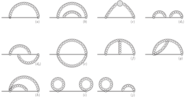
Figure 6.1: Diagrams relevant to the leading order and next-to-leading order evaluation of $Z_{g}$. Eq. (4.108). External grey blobs denote $F^{-\perp}$ insertions whereas internal grey blobs denote self energies. The solid lines represent Wilson lines and the curly lines a gauge boson.

6.1 Calculation Setup

We dive straight into the computation of the various diagrams, listed in Fig. 6.1. While in theory, the vacuum result should be subtracted from each diagram, we neglect this term throughout the chapter, as it vanishes in DR anyway.

Diagram $(a)$ just gives the LO contribution to $Z_{g}$, which we rewrite here for convenience [279, 274]

$$Z_{g}^{(a)}=\frac{T^{2}}{6}.$$ (6.3)

We now proceed to the arduous task of computing all of the NLO diagrams.

6.1.1 Diagram $(c)$

In Sec. 4.4.2, we computed the EQCD counterpart of diagram $(a)$. Diagram $(c)$ has the same structure, albeit with an extra self-energy insertion. We can thus pick up from Eq. (4.111), writing

$$Z_{g}^{(c)} =-2\int_{0}^{\infty}dx^{+}\int_{K}x^{+}e^{-ik^{-}x^{+}}(k^{-2}G_{>}^{xx}(K)-2k^{x}k^{-}G_{>}^{x-}(K)+{k^{x}}^{2}G_{>}^{--}(K))$$

$$=2\int_{K}\frac{1}{(k^{-}-i\varepsilon)^{2}}(k^{-2}G_{>}^{xx}(K)-2k^{x}k^{-}G_{>}^{x-}(K)+{k^{x}}^{2}G_{>}^{--}(K))$$ (6.4)

$$=2\int_{K}\frac{1+n_{\text{B}}(k^{0})}{(k^{-}-i\varepsilon)^{2}}(k^{-2}(G_{R}^{xx}(K)-G_{A}^{xx}(K))-2k^{x}k^{-}(G_{R}^{x-}(K)-G_{A}^{x-}(K))$$

$$+{k^{x}}^{2}(G_{R}^{--}(K)-G_{A}^{--}(K)))$$

$$=2\int_{K}\frac{1+n_{\text{B}}(k^{0})}{(k^{-}-i\varepsilon)^{2}}(F_{R}(K)-F_{A}(K))$$ (6.5)

where, in contrast to Eq. (4.111),

$$F_{R/A}(K) =\frac{i}{(K^{2}+i\varepsilon k^{0})^{2}}\big{(}k^{-2}\Pi^{xx}_{R/A}(K)-2k^{x}k^{-}(\Pi^{0x}_{R/A}(K)-\Pi^{zx}_{R/A}(K))$$

$$+{k^{x}}^{2}(\Pi^{00}_{R/A}(K)+\Pi^{zz}_{R/A}(K)-2\Pi^{z0}_{R/A}(K))\big{)}.$$ (6.6)

It is then useful to decompose the self-energies in terms of their longitudinal and transverse components

$$\Pi^{R/A}_{\mu\nu}(K)=P^{L}_{\mu\nu}(K)\Pi^{R/A}_{L}(K)+P^{T}_{\mu\nu}(K)\Pi^{R/A}_{T}(K)$$ (6.7)

where $P^{L}_{\mu\nu}$ and $P^{T}_{\mu\nu}$ are defined in Eqs. (4.79) and  (4.80) respectively. Making use of those same equations then leads to

$$F_{R/A}(K)= =\frac{i}{(K^{2}+i\varepsilon k^{0})^{2}}\bigg{[}k^{-2}\bigg{(}\Pi_{L}^{R}(K)\frac{k_{\perp}^{2}}{k^{2}}\bigg{)}$$

$$-2k^{x}k^{-}\bigg{(}\Pi_{L}^{R/A}(K)\Big{(}\frac{k^{x}k^{z}}{q^{2}}-\frac{k^{x}k^{-}}{K^{2}}\Big{)}-\Pi_{T}^{R/A}(K)\frac{k^{x}k^{z}}{q^{2}}\bigg{)}$$

$$+{k^{x}}^{2}\bigg{(}\Pi_{L}^{R/A}(K)\Big{(}1-\frac{k_{\perp}^{2}}{k^{2}}+\frac{k^{2}-2k^{0}k^{z}+{k^{z}}^{2}}{K^{2}}\Big{)}+\Pi_{T}^{R/A}(K)\frac{k_{\perp}^{2}}{k^{2}}\bigg{)}\bigg{]}$$

$$=\frac{i}{(K^{2}+i\varepsilon k^{0})^{2}}\bigg{[}k^{-2}\Pi_{T}^{R/A}(K)+\frac{{k^{x}}^{2}K^{2}}{k^{2}}(\Pi_{L}^{R/A}(K)-\Pi_{T}^{R/A}(K))\bigg{]},$$ (6.8)

which in turn results in

$$Z_{g}^{(c)} =i\int_{K}\frac{1+n_{\mathrm{B}}(k^{0})}{(k^{-}-i\varepsilon)^{2}}\bigg{[}\frac{2k^{-2}\Pi_{T}^{R}(K)}{(K^{2}+i\varepsilon k^{0})^{2}}+\frac{k_{\perp}^{2}(\Pi_{L}^{R}(K)-\Pi_{T}^{R}(K))}{k^{2}(K^{2}+i\varepsilon k^{0})}-\frac{2k^{-2}\Pi_{T}^{A}(K)}{(K^{2}-i\varepsilon k^{0})^{2}}$$

$$-\frac{k_{\perp}^{2}(\Pi_{L}^{A}(K)-\Pi_{T}^{A}(K))}{k^{2}(K^{2}-i\varepsilon k^{0})}\bigg{]}.$$ (6.9)

It is convenient to divide up the terms as follows

$$Z_{g}^{(c)}\equiv Z_{g\,k^{-2}}^{(c)}+Z_{g\,\text{L}-\text{T}}^{(c)}.$$ (6.10)

We find this to be a good stopping point, before matching the IR divergences of the expression above to those coming from the EQCD calculation in Sec. 6.3.

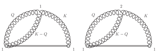
Figure 6.2: Different topologies associated with diagram $(g)$ with momentum flowing from left to right. The “1, 2” labels indicate the branch of the Schwinger-Keldysh contour from which the vertices are being pulled.

6.1.2 Diagram $(g)$

For the computation of diagram $(g)$, working in the 1/2 basis there are two possible thermal assignments, shown in Fig. 6.2. We start with the left diagram

$$Z_{g}^{(g)\,1} =-\frac{2}{d_{A}}\int_{0}^{\infty}dx^{+}x^{+}\bigg{\langle}\Big{[}\partial^{-}A^{x,a}_{1}(x^{+})-\partial^{x}A^{-,a}_{1}(x^{+})\Big{]}gf^{abc}A^{-,b}_{1}(0)A^{x,c}_{1}(0)\bigg{\rangle}^{1}$$

$$=-\frac{2gf^{abc}}{d_{A}}\int_{0}^{\infty}dx^{+}x^{+}\int_{K}e^{-k^{-}x^{+}}\bigg{\langle}\Big{[}-ik^{-}A^{x,a}_{1}+k^{x}A^{-,a}_{1}\Big{]}A^{-,b}_{1}A^{x,c}_{1}(0)\bigg{\rangle}^{1},$$ (6.11)

where the 1 subscripts on the gauge fields indicate that they are located on the time-ordered branch of the Schwinger-Keldysh contour (see Fig. 4.1). The 1 superscript on the angled bracket indicates that the thermal expectation value is to be evaluated with the three-gluon vertex of type 1. Upon evaluating the expectation value, we get

$$Z_{g}^{(g)\,1} =-\frac{2gf^{abc}}{d_{A}}\int_{0}^{\infty}dx^{+}x^{+}\int_{K,Q}e^{-ik^{-}x^{+}}\;\left(gf^{abc}\;V_{\alpha\beta\gamma}(Q,K-Q,-K)\right)$$

$$\times\Big{[}\left(-\eta^{-\alpha}G_{F}(Q)\right)\left(-\eta^{x\beta}G_{F}(K-Q)\right)\left(-ik^{-}\left(-\eta^{x\gamma}G_{F}(K)\right)+ik^{x}\left(-\eta^{-\gamma}G_{F}(K)\right)\right)\Big{]}$$

$$=-2ig^{2}C_{A}\int_{0}^{\infty}dx^{+}x^{+}\int_{K,Q}e^{-ik^{-}x^{+}}\;\Big{[}G_{F}(Q)G_{F}(K-Q)k^{-}G_{F}(K)V_{+xx}(Q,K-Q,-K)$$

$$\hskip 5.0pt-G_{F}(Q)G_{F}(K-Q)k^{x}G_{F}(K)V_{+x+}(Q,K-Q,-K)\Big{]}$$ (6.12)

From Eq. (A.2), we see that the second term vanishes. Moreover,

$$\int_{0}^{\infty}dx^{+}x^{+}e^{-ik^{-}x^{+}}=-\frac{1}{(k^{-}-i\varepsilon)^{2}},$$ (6.13)

so that

$$Z_{g}^{(g)\,1}=2ig^{2}C_{A}\int_{K,Q}G_{F}(Q)G_{F}(K-Q)G_{F}(K)\left(\frac{k^{-}q^{-}}{(k^{-}-i\varepsilon)^{2}}-2\right).$$ (6.14)

Now, let us repeat the same procedure for the vertex assigned to the 2-branch of the Schwinger-Keldysh contour (Fig.6.2-right)

$$Z_{g}^{(g)\,2} =-\frac{2}{d_{A}}\int_{0}^{\infty}dx^{+}x^{+}\bigg{\langle}\Big{[}\partial^{-}A^{x,c}_{1}(x^{+})-\partial^{x}A^{-,c}_{1}(x^{+})\Big{]}gf^{abc}A^{-,b}_{1}(0)A^{x,c}_{1}(0)\bigg{\rangle}^{2}$$

$$=-\frac{2}{d_{A}}\int_{0}^{\infty}dx^{+}x^{+}f^{abc}g^{2}\int_{K,Q}e^{-ik^{-}x^{+}}\left(-f^{abc}V_{\alpha\beta\gamma}(Q,K-Q,-K)\right)$$

$$\times\Big{[}\left(-\eta^{-\alpha}G_{<}(Q)\right)\left(-\eta^{x\beta}G_{<}(K-Q)\right)\left(-ik^{-}\left(-\eta^{x\gamma}G_{<}(K)\right)+ik^{x}\left(-\eta^{-\gamma}G_{<}(K)\right)\right)\Big{]}$$

$$=-2ig^{2}C_{A}\int_{K,Q}G_{<}(Q)G_{<}(K-Q)G_{>}(K)\left(\frac{k^{-}q^{-}}{(k^{-}-i\varepsilon)^{2}}-2\right).$$ (6.15)

To get the full contribution to $Z_{g}^{(g)}$, we need to add Eqs. (6.14) and Eq. (6.15) along with the mirror image of each diagram from Fig.6.2. While the mirror of Fig.6.2-left gives the same contribution as Eq. (6.14), to get the mirror of Fig.6.2-right, we should take Eq. (6.15) and make the replacement $G_{<}(Q)G_{<}(K-Q)G_{>}(K)\rightarrow G_{>}(Q)G_{>}(K-Q)G_{<}(K)$. This leaves us with

$$Z^{(g)}_{g} =2ig^{2}C_{A}\int_{K,Q}\left(\frac{q^{-}}{k^{-}-i\varepsilon}-2\right)\Big{[}2G_{F}(Q)G_{F}(K-Q)G_{F}(K)-G_{>}(Q)G_{>}(K-Q)G_{<}(K)$$

$$-G_{<}(Q)G_{<}(K-Q)G_{>}(K)\Big{]}$$ (6.16)

In order to simplify things, we employ the amputated self-energy-like objects defined in App. D.1, which allow us to rewrite Eq. (6.16) as

$$Z^{(g)}_{g} =2ig^{2}C_{A}\int_{K,Q}\left(\frac{q^{-}}{k^{-}-i\varepsilon}-2\right)\Big{[}\Big{(}2\widetilde{\Pi_{aa}}(K)+\widetilde{\Pi_{R}}(K)+\widetilde{\Pi_{A}}(K)\Big{)}G_{F}(K)$$

$$-\widetilde{\Pi_{>}}(K)G_{<}(K)-\widetilde{\Pi_{<}}(K)G_{>}(K)\Big{]}.$$ (6.17)

In arriving at the above expression, one must invoke that the closed loops of causality vanish (see Sec. 4.2.3). Specifically, this argument applies to the terms containing $G_{R}(Q)G_{A}(K-Q),\,G_{A}(Q)G_{R}(K-Q)$. It then suffices to use the KMS-like relations in App. D.1 to arrive at

$$Z^{(g)}_{g}=4ig^{2}C_{A}\int_{K,Q}\left(\frac{q^{-}}{k^{-}-i\varepsilon}-2\right)\left(1+n_{\text{B}}(k^{0})\right)\left(\widetilde{\Pi_{R}}(K)G_{R}(K)-\widetilde{\Pi_{A}}(K)G_{A}(K)\right).$$ (6.18)

We halt with the evaluation at this stage. Indeed, we will see that this contribution cancels with the one coming from diagram $(f)$ in Sec. 6.2.2.

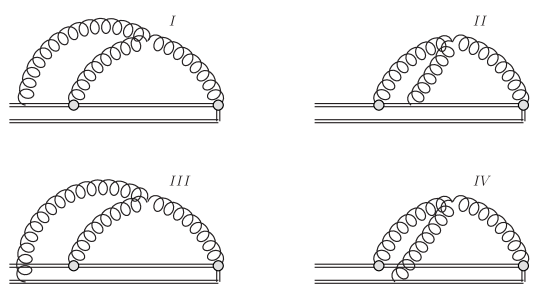
Figure 6.3: Different topologies associated with diagram $(f)$ with momentum flowing from left to right. In all cases, we take the propagator attached to the Wilson line (as opposed to the $F$ operator insertions) to have momentum $K-Q$.

6.1.3 Diagram $(f)$

This is the only non-vanishing diagram where the gluons are being pulled from the Wilson line itself. The corresponding contributions to this diagram are listed in Fig. 6.3. We then have $8$ possible assignments overall, since each of these $4$ subdiagrams can have either a $1$ or $2$ labelling for the three-gluon vertex.

Since it is an $A^{-}$ field that is being pulled from the Wilson line (see Eq. (4.109)), we can conclude that in each subdiagram, the only contribution to the three-gluon vertex will be proportional to $\eta_{xx}$. We proceed to first compute the contribution from $Z_{g}^{f\,I}$, pointing to Fig. 6.3 for clarification about the labelling

$$Z_{g}^{(f)\,I} =\frac{-2}{d_{R}C_{R}}(ig)\int_{0}^{\infty}dx^{+}x^{+}\int_{-\infty}^{0}dy^{+}\bigg{[}\frac{if^{cba}}{4}\bigg{\langle}\partial^{-}A^{a,x}(x^{+})\partial^{-}A^{b,x}(0)A^{c,-}(y^{+})\bigg{\rangle}^{1}$$

$$+\frac{if^{acb}}{4}\bigg{\langle}\partial^{-}A^{a,x}(x^{+})\partial^{-}A^{b,x}(0)A^{c,-}(y^{+})\bigg{\rangle}^{2}\bigg{]}$$ (6.19)

where the two factors in parentheses out in front come from the colour trace and the Wilson line respectively. Then, Fourier transforming in a way that is consistent with the labelling convention mentioned in Fig. 6.3, we find

$$Z_{g}^{(f)\,I} =-\frac{2ig}{d_{R}C_{R}}\int_{0}^{\infty}dx^{+}x^{+}\int_{-\infty}^{0}dy^{+}\int_{K,Q}k^{-}q^{-}e^{-ik^{-}x^{+}}e^{-i(q^{-}-k^{-})y^{+}}$$

$$\times\bigg{[}\frac{if^{cba}}{4}\bigg{\langle}A^{a,x}(K)A^{b,x}(Q)A^{c,-}(K-Q)\bigg{\rangle}^{1}+\frac{if^{acb}}{4}\bigg{\langle}A^{a,x}(K)A^{b,x}(Q)A^{c,-}(K-Q)\bigg{\rangle}^{2}\bigg{]}$$

$$=-\frac{2ig}{d_{R}C_{R}}\int_{K,Q}\frac{q^{-}}{(k^{-}-i\varepsilon)(k^{-}-q^{-}-i\varepsilon)}$$

$$\times\bigg{[}\frac{if^{cba}}{4}\bigg{\langle}A^{a,x}(K)A^{b,x}(Q)A^{c,-}(K-Q)\bigg{\rangle}^{1}+\frac{if^{acb}}{4}\bigg{\langle}A^{a,x}(K)A^{b,x}(Q)A^{c,-}(K-Q)\bigg{\rangle}^{2}\bigg{]}$$

$$=ig^{2}C_{A}\int_{K,Q}\frac{q^{-}(k^{-}+q^{-})}{(k^{-}-i\varepsilon)(k^{-}-q^{-}-i\varepsilon)}\Big{[}-G_{F}(Q)G_{F}(K)G_{F}(K-Q)$$

$$+G_{>}(Q)G_{<}(K)G_{>}(K-Q)\Big{]}.$$ (6.20)

Note that the thermal assignments are separated by a minus: this is because, in the second, we are pulling a 2 vertex from the action. We can immediately then write down the expression for the contribution of the subdiagram with the gluon instead attached to the Wilson line directly below

$$Z_{g}^{(f)\,III} =-ig^{2}C_{A}\int_{K,Q}\frac{q^{-}(k^{-}+q^{-})}{(k^{-}-i\varepsilon)(k^{-}-q^{-}-i\varepsilon)}\Big{[}-G_{F}(Q)G_{F}(K)G_{<}(K-Q)$$

$$+G_{>}(Q)G_{<}(K)G_{\bar{F}}(K-Q)\Big{]}.$$ (6.21)

The minus sign out in front can be attributed to the fact that in this case, the limits of the $y^{+}$ integral are switched. The thermal assignments are of course different in this subdiagram, since the lower Wilson line is anti-time-ordered. Combining the two subdiagrams then yields, after some algebra

$$Z_{g}^{(f)\,I}+Z_{g}^{(f)\,III} =-ig^{2}C_{A}\int_{K,Q}\frac{q^{-}(k^{-}+q^{-})}{(k^{-}-i\varepsilon)(k^{-}-q^{-}-i\varepsilon)}G_{R}(K-Q)\Big{[}G_{rr}(Q)G_{R}(K)$$

$$+G_{rr}(K)G_{A}(Q)+\frac{1}{2}\left(G_{R}(K)G_{R}(Q)+G_{A}(K)G_{A}(Q)\right)\Big{]}$$ (6.22)

the last two terms are scaleless and therefore vanish in dimensional regularisation.

Moving onto the subdiagram where the gluon is attached to the line between the two $F$ insertions, we have

$$Z_{g}^{(f)\,II} =\frac{-2}{d_{R}C_{R}}(ig)\int_{0}^{\infty}dx^{+}x^{+}\int_{0}^{x^{+}}dy^{+}\int_{K,Q}k^{-}q^{-}e^{-ik^{-}x^{+}}e^{-i(q^{-}-k^{-})y^{+}}$$ (6.23)

$$\times\bigg{[}\frac{if^{cba}}{4}\bigg{\langle}A^{a,x}(K)A^{b,-}(K-Q)A^{c,x}(Q)\bigg{\rangle}^{1}+\frac{if^{bca}}{4}\bigg{\langle}A^{a,x}(K)A^{b,-}(K-Q)A^{c,x}(Q)\bigg{\rangle}^{2}\bigg{]}$$

$$=\frac{2g}{d_{R}C_{R}}\int_{K,Q}\frac{1}{q^{-}-k^{-}}\left(\frac{q^{-}}{k^{-}-i\varepsilon}-\frac{k^{-}}{q^{-}-i\varepsilon}\right)$$

$$\times\bigg{[}\frac{if^{cba}}{4}\bigg{\langle}A^{a,x}(K)A^{b,-}(K-Q)A^{c,x}(Q)\bigg{\rangle}^{1}+\frac{if^{bca}}{4}\bigg{\langle}A^{a,x}(K)A^{b,-}(K-Q)A^{c,x}(Q)\bigg{\rangle}^{2}\bigg{]}$$

$$=-ig^{2}C_{A}\int_{K,Q}(k^{-}+q^{-})\left(\frac{1}{k^{-}-i\varepsilon}+\frac{1}{q^{-}-i\varepsilon}\right)\Big{[}-G_{F}(Q)G_{F}(K)G_{F}(K-Q)$$

$$+G_{>}(Q)G_{<}(K)G_{>}(K-Q)\Big{]}.$$ (6.24)

In this case, the corresponding diagram with the gluon attached below has the same sign, due to relative minuses coming from both the colour trace and the inversion of the limits on the $y^{+}$ integral. Thus,

$$Z_{g}^{(f)\,IV} =-ig^{2}C_{A}\int_{K,Q}(k^{-}+q^{-})\left(\frac{1}{k^{-}-i\varepsilon}+\frac{1}{q^{-}-i\varepsilon}\right)\Big{[}-G_{F}(Q)G_{F}(K)G_{<}(K-Q)$$

$$+G_{>}(Q)G_{<}(K)G_{\bar{F}}(K-Q)\Big{]}.$$ (6.25)

Together these two add to give,

$$Z_{g}^{(f)\,II} +Z_{g}^{(f)\,IV}=ig^{2}C_{A}\int_{K,Q}(k^{-}+q^{-})\left(\frac{1}{k^{-}-i\varepsilon}+\frac{1}{q^{-}-i\varepsilon}\right)\Big{\{}G_{A}(K-Q)\Big{[}\frac{1}{2}G_{A}(Q)G_{R}(K)$$

$$+2G_{rr}(K)G_{rr}(Q)+G_{rr}(K)G_{R}(Q)\Big{]}+2G_{rr}(K-Q)\Big{[}\frac{1}{2}G_{R}(K)G_{R}(Q)+G_{rr}(Q)G_{R}(K)$$

$$+G_{rr}(K)G_{A}(Q)\Big{]}\Big{\}}$$

$$=ig^{2}C_{A}\int_{K,Q}\frac{k^{-}+q^{-}}{k^{-}-i\varepsilon}$$

$$\times\Big{\{}4\left(\frac{1}{2}+n_{\text{B}}(k^{0})\right)\Big{[}G_{R}(K)\widetilde{\Pi_{R}}(K)-G_{A}(K)\widetilde{\Pi_{A}}(K)\Big{]}+2G_{R}(K)\widetilde{\Pi_{R}}(K)$$

$$-G_{R}(K)\Big{[}G_{R}(K-Q)G_{rr}(Q)+\frac{1}{2}G_{R}(K-Q)G_{R}(Q)\Big{]}\Big{\}}$$ (6.26)

where we have made use of the “amputated self-energy” relations from App. D.1. We come back to Eqs. (6.22) and  (6.26) in Sec. 6.2.1.

6.1.4 Diagrams $(b),\,(d_{1}),\,(d_{2}),\,(e),\,(h),\,(i),\,(j)$

It suffices to write down the expression for diagram $(b)$

$$Z_{g}^{(b)} =-\frac{\mathcal{2C}(ig)^{2}}{d_{R}C_{F}}\int_{0}^{\infty}dx^{+}x^{+}\int_{0}^{x^{+}}dy^{+}\int_{0}^{y^{+}}dz^{+}\Bigl{\langle}\Big{(}\partial^{-}A^{x}_{a}(x^{+})-\partial^{x}A^{-}_{a}(x^{+})\Big{)}\Big{(}\partial^{-}A^{x}_{a}(0)-\partial^{x}A^{-}_{a}(0)\Big{)}\Bigr{\rangle}$$

$$\times\Bigl{\langle}A^{-}_{b}(y^{+})A^{-}_{b}(z^{+})\Bigr{\rangle},$$ (6.27)

where $\mathcal{C}$ is some non-zero colour factor. In Feynman gauge, the $\Bigl{\langle}A^{-}_{b}(y^{+})A^{-}_{b}(z^{+})\Bigr{\rangle}$ factor above will inevitably produce an $\eta^{--}$, from which we can conclude that this diagram vanishes. The other diagrams $(b),\,(d_{1}),\,(d_{2}),\,(e),\,(h),\,(i),\,(j)$ then vanish for the same reason as they only contain terms proportional to either $\Bigl{\langle}A^{-}A^{-}\Bigr{\rangle}$ or $\Bigl{\langle}A^{-}A^{x}\Bigr{\rangle}$, the latter of which is also zero in Feynman gauge.

6.2 Proof of $Z_{g}^{(f)}+Z_{g}^{(g)}=0$

We provide two arguments, supporting the claim that in Feynman gauge, we need only consider the contribution from diagram $(c)$ in Fig. 6.1.

6.2.1 Proof from the Correlator

Let us start by looking at Eq. (4.69) and writing

$$Z_{g}=-\frac{1}{d_{R}C_{R}}\int_{0}^{\infty}dx^{+}x^{+}\,\Tr\,\Bigl{\langle}U_{R}(-\infty;x^{+})F^{-\perp}(x^{+})\,U_{R}(x^{+};0)\,F^{-\perp}(0)U_{R}(0;-\infty)\Bigr{\rangle},$$ (6.28)

where $F^{-\perp}F^{-\perp}$ is taken to mean $F^{-x}F^{-x}+F^{-y}F^{-y}$. Continuing onwards, let us recast Eq. (4.69) as a double integral, using translation invariance

$$Z_{g} =-\frac{1}{d_{R}C_{R}}\int_{0}^{\infty}dx^{+}\int_{0}^{x^{+}}dy^{+}\Tr\,\Bigl{\langle}U_{R}(-\infty;x^{+}+y^{+})F^{-\perp}(x^{+}+y^{+})\,U_{R}(x^{+}+y^{+};y^{+})\,F^{-\perp}(y^{+})$$

$$\times U_{R}(y^{+};-\infty)\Bigr{\rangle},$$

$$=-\frac{1}{d_{R}C_{R}}\int_{0}^{\infty}dx^{+}\int_{0}^{x^{+}/2}\!dy^{+}\,\Tr\,\Bigl{\langle}U_{R}(-\infty;x^{+})F^{-\perp}(x^{+})\,U_{R}(x^{+};y^{+})\,F^{-\perp}(y^{+})U_{R}(y^{+};-\infty)\Bigr{\rangle},$$ (6.29)

where we have shifted $x^{+}$ in going to the second line. We now rewrite $Z_{g}$ as

$$Z_{g}\equiv Z_{g}^{\perp\perp}+Z_{g}^{\perp-}+Z_{g}^{-\perp}+Z_{g}^{--},$$ (6.30)

with the apex labelling to be elaborated on momentarily. By calling on a method introduced in [282]: we rewrite

$$F^{-\perp}=-\partial^{\perp}A^{-}+[D^{-},A^{\perp}].$$ (6.31)

The equation of motion of the Wilson line (see Eq. (B.8)), $D^{-}_{x^{+}}U(x^{+};y^{+})=0$ can then be used to rewrite the commutator as a total derivative, i.e.

$$U_{R}(a;x^{+})[D^{-},A^{\perp}(x^{+})]U_{R}(x^{+};b)=\frac{d}{dx^{+}}[U_{R}(a;x^{+})\,A^{\perp}(x^{+})\,U_{R}(x^{+};b)].$$ (6.32)

This should shed light on the labelling in Eq. (6.30): the apexes there denote whether the $-\partial^{\perp}A^{-}$ (^⟂) or the $[D^{-},A^{\perp}]$ component (^-) of the field strength tensor has been taken.

Starting with the first term from Eq. (6.30),

$$Z_{g}^{\perp\perp}=-\frac{1}{d_{R}C_{R}}\int_{0}^{\infty}dx^{+}x^{+}\,\Tr\,\Bigl{\langle}U_{R}(-\infty;x^{+})\partial^{\perp}A^{-}(x^{+})\,U_{R}(x^{+};0)\,\partial^{\perp}A^{-}(0)U_{R}(0;-\infty)\Bigr{\rangle}.$$ (6.33)

Whereas for the second term, we have, employing Eq. (6.32)

$$Z_{g}^{\perp-} =\frac{1}{d_{R}C_{R}}\int_{0}^{\infty}dx^{+}\,\Tr\,\Bigl{\langle}U_{R}(-\infty;x^{+})\partial^{\perp}A^{-}(x^{+})\,U_{R}(x^{+};x^{+}/2)\,\Big{[}A^{\perp}(x^{+}/2)U_{R}(x^{+}/2;0)$$

$$-U_{R}(x^{+}/2;0)A^{\perp}(0)\Big{]}U_{R}(0;-\infty)\Bigr{\rangle}.$$ (6.34)

Translation invariance dictates that for the first term

$$\Bigl{\langle}U_{R}(-\infty;x^{+})\partial^{\perp}A^{-}(x^{+})\,U_{R}(x^{+};x^{+}/2)\,A^{\perp}(x^{+}/2)U_{R}(x^{+}/2;-\infty)\Bigr{\rangle}=\Bigl{\langle}U_{R}(-\infty;x^{+}/2)$$

$$\times\partial^{\perp}A^{-}(x^{+}/2)\,U_{R}(x^{+}/2;0)\,A^{\perp}(0)U_{R}(0;-\infty)\Bigr{\rangle}.$$ (6.35)

By aptly redefining the integration variable for this term one finds that

$$Z_{g}^{\perp-}=\frac{1}{d_{R}C_{R}}\int_{0}^{\infty}dx^{+}\,\Tr\,\Bigl{\langle}U_{R}(-\infty;x^{+})\partial^{\perp}A^{-}(x^{+})\,U_{R}(x^{+};0)\,A^{\perp}(0)U_{R}(0;-\infty)\Bigr{\rangle}.$$ (6.36)

For its counterpart we have

$$Z_{g}^{-\perp}=-\frac{1}{d_{R}C_{R}}\int_{0}^{\infty}dy^{+}\,\Tr\,\Bigl{\langle}U_{R}(-\infty;2y^{+})A^{\perp}(2y^{+})\,U_{R}(2y^{+};y^{+})\,\partial^{\perp}A^{-}(y^{+})U_{R}(y^{+};-\infty)\Bigr{\rangle}.$$ (6.37)

where we used the fact that, in a non-singular gauge, $A^{\perp}(\infty)=0$. By applying translation invariance and relabeling $y^{+}$ into $x^{+}$ this becomes

$$Z_{g}^{-\perp}=-\frac{1}{d_{R}C_{R}}\int_{0}^{\infty}dx^{+}\,\Tr\,\Bigl{\langle}U_{R}(-\infty;x^{+})A^{\perp}(x^{+})\,U_{R}(x^{+};0)\,\partial^{\perp}A^{-}(0)U_{R}(0;-\infty)\Bigr{\rangle}.$$ (6.38)

Finally, for the term with both commutators, we find

$$Z_{g}^{--}=\frac{1}{d_{R}C_{R}}\,\Tr\,\Bigl{\langle}U_{R}(-\infty;0)A^{\perp}(0)\,A^{\perp}(0)U_{R}(0;-\infty)\Bigr{\rangle},$$ (6.39)

where we have again set the boundary term at infinity to zero.

At this point, we recall that in Feynman gauge the ^– gluon propagator vanishes and furthermore, that a three-gluon vertex with more than one ^- gluon does as well. Let us then consider Eq. (6.33): at LO it must vanish in Feynman gauge. At NLO it can only contribute to part of diagram $(c)$. Note however that the Wilson lines cannot contribute on their own for the same reasons outlined in Sec. (6.1.4). Moreover, there cannot be a contribution of the form of diagram $(g)$ as the $gA^{-}A^{\perp}$ part of the covariant derivative has been removed from the correlator through the previous manipulations.

Similar arguments can be safely applied to Eqs. (6.36) and (6.38): they also have a vanishing $(f)$ contribution and they correspond to the mixed $G^{x-}_{>}(K)$ terms in Eq. (6.4).

Eq. (6.39) does not vanish at LO: it corresponds precisely to diagram $(a)$. At NLO it too contains a contribution to $(c)$, that proportional to $G^{xx}_{>}(K)$ terms in Eq. (6.4). It also contains the only contribution directly involving the Wilson lines, as either of them can source an $A^{-}$ gluon that can connect with a three-gluon vertex to the two $A^{\perp}$ ones. However, that would give rise to the following colour structure

$$\mathcal{C}=f^{abc}A^{\perp\,a}A^{\perp\,b}A^{-\,c},$$ (6.40)

which vanishes, due to the symmetric (anti-symmetric) nature of $A^{\perp\,a}A^{\perp\,b}$ ($f^{abc}$). Given that, through this reorganisation, we only encounter non-zero contributions from diagram $(c)$, we conclude that the respective contributions from diagrams $(f)$ and $(g)$ must cancel each other. We further back up this argument with a direct diagrammatic proof in the next section.

6.2.2 Diagrammatic Proof

Coming back to Eq. (6.22), we note that by suitably relabelling momenta, we can drastically simplify this expression: let us start by considering the second term and relabeling $K-Q\rightarrow K,\\ Q\rightarrow Q-K\,,K\rightarrow Q$. This yields

$$Z_{g}^{(f)\,I}+Z_{g}^{(f)\,III} =-ig^{2}C_{A}\int_{K,Q}\Big{[}\frac{q^{-}(k^{-}+q^{-})}{(k^{-}-i\varepsilon)(k^{-}-q^{-}-i\varepsilon)}+\frac{(q^{-}-k^{-})(2q^{-}-k^{-})}{(q^{-}-i\varepsilon)(k^{-}-i\varepsilon)}\Big{]}$$

$$\times G_{R}(K-Q)G_{rr}(Q)G_{R}(K)$$

$$=-ig^{2}C_{A}\int_{K,Q}\Big{[}\frac{q^{-}(k^{-}+q^{-})}{(k^{-}-i\varepsilon)(k^{-}-q^{-}-i\varepsilon)}+\frac{2q^{-}}{(k^{-}-i\varepsilon)}\Big{]}$$

$$\times G_{R}(K-Q)G_{rr}(Q)G_{R}(K)$$ (6.41)

where in going to the second line, we have used that we can throw away any terms in the second term with a factor of $k^{-}$ in the numerator, since the $k^{-}$ integral can then be closed in the upper half plane. We then perform another relabelling of the momenta in the second term: $K-Q\rightarrow K\,,\,Q\rightarrow-Q\,,\,K\rightarrow K-Q$, under which the multiplied propagators are invariant

$$Z_{g}^{(f)\,I}+Z_{g}^{(f)\,III} =-ig^{2}C_{A}\int_{K,Q}\Big{[}\frac{q^{-}(k^{-}+q^{-})}{(k^{-}-i\varepsilon)(k^{-}-q^{-}-i\varepsilon)}-\frac{2q^{-}}{(k^{-}-q^{-}-i\varepsilon)}\Big{]}$$

$$\times G_{R}(K-Q)G_{rr}(Q)G_{R}(K)$$

$$=ig^{2}C_{A}\int_{K,Q}\frac{q^{-}}{k^{-}-i\varepsilon}G_{R}(K-Q)G_{rr}(Q)G_{R}(K).$$ (6.42)

At this point, let us go back and look at the expression coming from the evaluation of diagram $(g)$, Eq. (6.18) and relabel so that $Q\rightarrow K-Q\,,\,K-Q\rightarrow Q\,,\,K\rightarrow K$, yielding

$$Z^{(g)}_{g}=-4ig^{2}C_{A}\int_{K,Q}\frac{k^{-}+q^{-}}{k^{-}-i\varepsilon}\left(1+n_{\text{B}}(k^{0})\right)\left(\widetilde{\Pi_{R}}(K)G_{R}(K)-\widetilde{\Pi_{A}}(K)G_{A}(K)\right).$$ (6.43)

which of course resembles what we have in Eq. (6.26). Let us then add both contributions to see if they cancel

$$Z_{g}^{(f)\,II} +Z_{g}^{(f)\,V}+Z_{g}^{(g)}=ig^{2}C_{A}\int_{K,Q}\frac{k^{-}+q^{-}}{k^{-}-i\varepsilon}\Big{\{}2\widetilde{\Pi_{A}}(K)G_{A}(K)$$

$$-G_{R}(K)G_{R}(K-Q)G_{rr}(Q)-\frac{1}{2}G_{R}(K)G_{R}(K-Q)G_{R}(Q)\Big{\}}.$$ (6.44)

The first term above is advanced in $k^{-}$, so we can just close the integration in the lower half plane to see that it vanishes. Likewise, for the $k^{-}/(k^{-}-i\varepsilon)$ proportional part of the second term, we can close the $k^{-}$ integration in the upper half plane to see that it does not contribute. The third term will vanish after a suitable relabelling of the momenta whereas the $q^{-}/(k^{-}-i\varepsilon)$ part of the second term cancels against what we found in Eq. (6.42).

Alternatively, we could invoke the ideas from Sec. 4.3 since in the case of the second and third term, the propagators are lightlike separated and are thus retarded in both $k^{-}$ and $k^{+}$. The $1/(k^{-}-i\varepsilon)$ out in front means that we cannot close the $k^{-}$ in the upper half plane without picking up a contribution there. However, there are no such extra poles in $k^{+}$ and so we can therefore close the $k^{+}$ integration in the upper half-plane.

In any case, we undoubtedly conclude

$$Z_{g}^{(f)}+Z_{g}^{(g)}=0.$$ (6.45)

6.3 Matching from Full QCD

In this section, we compute zero-mode contributions from the gluonic part of diagram $(c)$ and thus $Z_{g}$, before checking that they cancel with the corresponding EQCD contributions in the next section. Throughout, for consistency’s sake, we set up the integration so that the $K$ integration is done in DR whereas the $Q$ integration is done in $4$ dimensions. It is useful in this context to think of the contributions to $Z_{g}$, in diagram $(c)$ as a double sum over Matsubara modes, one sum coming from $k^{0}$ and the other coming from $q^{0}$. Since EQCD is a theory of soft modes, it only accounts for the zero modes of the full theory. It is then natural to expect corresponding divergences on the full QCD side to show up in the term of the double sum with both zero modes. Indeed, this is physically what happens. However, this double zero mode term will give no contribution in DR, as it is the result of a scaleless integral. Thus, mathematically, what happens is that the divergence gets shifted from the $n=0\,,\,n=0$ term to the $n=0\,,\,n\neq 0$ terms. We make a point to organise things so the divergence comes from the zero mode associated with the momentum $K$.

We emphasise that we only need to do this matching for the gluonic contribution to $Z_{g}^{(c)}$ as EQCD only describes the dynamics of the gluonic zero modes.

6.3.1 $k^{-2}$ Piece

We begin by computing the $k^{-2}$ contribution, defined by Eqs. (6.9) and  (6.10). We moreover need the gluonic form of $\Pi_{T}^{R}(K)$, Eq. (D.12)

$$Z^{(c)}_{g\,k^{-2}\,G} =i\frac{g^{2}C_{A}}{8\pi^{2}}\int_{K}\int_{0}^{\infty}dq\frac{(1+n_{B}(k^{0}))}{k^{3}}n_{B}(q)\Bigg{[}\frac{1}{(K^{2}+i\varepsilon k^{0})^{2}}\Bigg{(}8qk(k^{2}+k_{0}^{2})$$

$$-K^{2}(4q^{2}+3k^{2}+k_{0}^{2})\left(\ln\frac{k_{0}+k-2q+i\varepsilon}{k_{0}-k-2q+i\varepsilon}+\ln\frac{k_{0}-k+2q+i\varepsilon}{k_{0}+k+2q+i\varepsilon}\right)$$

$$-4qk_{0}K^{2}\left(\ln\frac{k_{0}+k+i\varepsilon}{k_{0}-k+i\varepsilon}+\ln\frac{k_{0}-k+2q+i\varepsilon}{k_{0}+k+2q+i\varepsilon}-\ln\frac{k_{0}+k-2q+i\varepsilon}{k_{0}-k-2q+i\varepsilon}\right)\Bigg{)}-\text{adv.}\Bigg{]}$$ (6.46)

Let us then the write $k^{0}$ integral as a sum over the Matsubara modes. This leaves us with

$$Z^{(c)}_{g\,k^{-2}\,G} =-\frac{g^{2}C_{A}T}{8\pi^{2}}\sum_{n}\int_{k}\int_{0}^{\infty}dq\frac{1}{k^{3}}n_{B}(q)\frac{1}{(-\omega_{n}^{2}-k^{2})^{2}}\Bigg{(}8qk(k^{2}-\omega_{n}^{2})$$

$$-(-\omega_{n}^{2}-k^{2})(4q^{2}+3k^{2}-\omega_{n}^{2})\left(\ln\frac{i\omega_{n}+k-2q}{i\omega_{n}-k-2q}+\ln\frac{i\omega_{n}-k+2q}{i\omega_{n}+k+2q}\right)$$

$$-4iq\omega_{n}(-\omega_{n}^{2}-k^{2})\left(\ln\frac{i\omega_{n}+k}{i\omega_{n}-k}+\ln\frac{i\omega_{n}-k+2q}{i\omega_{n}+k+2q}-\ln\frac{i\omega_{n}+k-2q}{i\omega_{n}-k-2q}\right)\Bigg{)}.$$ (6.47)

Next, we extract the zero mode contribution

$$Z^{(c)}_{g\,k^{-2}\,G\,n=0}=-\frac{g^{2}C_{A}T}{8\pi^{2}}\int_{k}\int_{0}^{\infty}dq\frac{1}{k^{3}}n_{B}(k)\frac{1}{k^{4}}\Bigg{(}8qk^{3}+2k^{2}(4q^{2}+3k^{2})\ln\left|\frac{2q-k}{k+2q}\right|\Bigg{)}.$$ (6.48)

Before carrying out the integration in DR, it is first useful to rescale $k\rightarrow kq$ so that the integrations factorise, i.e

$$Z^{(c)}_{g\,k^{-2}\,G\,n=0} =-\frac{g^{2}C_{A}T}{8\pi^{2}}\Big{(}\frac{\bar{\mu}^{2}e^{\gamma_{E}}}{4\pi}\Big{)}^{\epsilon}\Big{(}\frac{2\pi^{\frac{d}{2}}}{\Gamma\left(\frac{d}{2}\right)(2\pi)^{d}}\Big{)}\int_{0}^{\infty}dk\int_{0}^{\infty}dq\frac{k^{d-1}}{k^{5}}\frac{q^{d+2}}{q^{5}}n_{B}(q)\Bigg{(}8k$$

$$+2(4+3k^{2})\ln\left|\frac{2-k}{k+2}\right|\Bigg{)}$$

$$=\frac{g^{2}C_{A}T^{2}}{32\pi^{2}}\bigg{[}-\frac{3}{\epsilon}-\left(7+6\ln\frac{\bar{\mu}}{4T}\right)\bigg{]},$$ (6.49)

where, as is specified in App. A, DR is carried out in $d=3-2\epsilon$ dimensions.

6.3.2 $\Pi_{L}-\Pi_{T}$ Piece

Let us start by writing the full contribution (i.e, that coming from all modes) using Eq.s (6.9) and  (D.14). This yields

$$Z^{(c)}_{g\,L-T\,G} =i\frac{g^{2}C_{A}}{16\pi^{2}}\int_{K}\int_{0}^{\infty}dq\frac{(1+n_{B}(k^{0}))}{k^{3}(k^{-}-i\varepsilon)^{2}}n_{B}(q)\Bigg{[}\frac{k_{\perp}^{2}}{k^{2}(K^{2}+i\varepsilon k^{0})}\Bigg{(}-8qk(3k_{0}^{2}-k^{2})$$

$$+K^{2}(12q^{2}-k^{2}+3k_{0}^{2})\left(\ln\frac{k_{0}+k-2q+i\varepsilon}{k_{0}-k-2q+i\varepsilon}+\ln\frac{k_{0}-k+2q+i\varepsilon}{k_{0}+k+2q+i\varepsilon}\right)$$

$$+12qk_{0}K^{2}\left(\ln\frac{k_{0}+k+i\varepsilon}{k_{0}-k+i\varepsilon}+\ln\frac{k_{0}-k+2q+i\varepsilon}{k_{0}+k+2q+i\varepsilon}-\ln\frac{k_{0}+k-2q+i\varepsilon}{k_{0}-k-2q+i\varepsilon}\right)\Bigg{)}-\text{adv.}\Bigg{]}.$$ (6.50)

After doing a Caron-Huot shift, i.e $k^{z}\rightarrow k^{z}+k^{0}$, we isolate the zero mode contribution by replacing $\int\frac{dk^{0}}{2\pi}$ with $iT\sum_{n}$ and then setting $\omega_{n}\rightarrow 0$. We are left with

$$Z^{(c)}_{g\,L-T\,G\,n=0} =-\frac{g^{2}C_{A}T}{16\pi^{2}}\int_{k}\int_{0}^{\infty}dq\frac{1}{k^{3}(k^{z}+i\varepsilon)^{2}}n_{B}(q)\frac{k_{\perp}^{2}}{k^{2}(-k^{2})}\Bigg{(}-8qk(-k^{2})$$

$$+(-k^{2})(12q^{2}-k^{2})\left(\ln\frac{k-2q}{-k-2q}+\ln\frac{-k+2q}{k+2q}\right)\Bigg{)}$$

$$=\frac{g^{2}C_{A}T}{16\pi^{2}}\int_{k}\int_{0}^{\infty}dq\frac{k_{\perp}^{2}}{k^{7}(k^{z}+i\varepsilon)^{2}}n_{B}(q)\Bigg{(}8qk^{3}-k^{2}(12q^{2}-k^{2})\left(2\ln|\frac{2q-k}{k+2q}\bigg{|}\right)\Bigg{)}.$$ (6.51)

In contrast to the previous piece, the integrand depends on the polar angle, $\theta$, which we deal with by making the substitution $x=\cos\theta$. The integral then yields

$$Z^{(c)}_{g\,L-T\,G\,n=0} =\frac{g^{2}C_{A}T}{16\pi^{2}}\left(\frac{\bar{\mu}^{2}e^{\gamma_{E}}}{4\pi}\right)^{\epsilon}\left(\frac{2\pi^{\frac{d-1}{2}}}{\Gamma\left(\frac{d-1}{2}\right)(2\pi)^{d}}\right)\int_{0}^{\infty}dk\int_{-1}^{1}dx\int_{0}^{\infty}dq\,n_{B}(q)k^{d-8}\frac{(1-x^{2})^{\frac{d-1}{2}}}{x^{2}}$$

$$\Bigg{(}8qk^{3}-k^{2}(12q^{2}-k^{2})\left(2\ln|\frac{2q-k}{k+2q}\bigg{|}\right)\Bigg{)}$$

$$=\frac{g^{2}C_{A}T}{16\pi^{2}}\left(\frac{\bar{\mu}^{2}e^{\gamma_{E}}}{4\pi}\right)^{\epsilon}\left(\frac{2\pi^{\frac{d-1}{2}}}{\Gamma\left(\frac{d-1}{2}\right)(2\pi)^{d}}\right)\int_{0}^{\infty}dk\int_{-1}^{1}dx\int_{0}^{\infty}dqT^{d-2}\frac{q^{d-7}}{e^{q}-1}k^{d-8}\frac{(1-x^{2})^{\frac{d-1}{2}}}{x^{2}}$$

$$\Bigg{(}8q^{4}k^{3}-2k^{2}q^{2}(12q^{2}-k^{2}q^{2})\ln|\frac{2-k}{k+2}\bigg{|}\Bigg{)}$$

$$=\frac{g^{2}C_{A}T^{d-1}}{16\pi^{2}}\left(\frac{\bar{\mu}^{2}e^{\gamma_{E}}}{4\pi}\right)^{\epsilon}\left(\frac{2\pi^{\frac{d-1}{2}}}{\Gamma\left(\frac{d-1}{2}\right)(2\pi)^{d}}\right)\int_{0}^{\infty}dk\int_{-1}^{1}dx\int_{0}^{\infty}dq\frac{q^{d-3}}{e^{q}-1}k^{d-6}\frac{(1-x^{2})^{\frac{d-1}{2}}}{x^{2}}$$

$$\Bigg{(}8k-2(12-k^{2})\ln|\frac{2-k}{k+2}\bigg{|}\Bigg{)}.$$ (6.52)

In the first line, we have dropped the $i\varepsilon$ piece since the $x$ dependent part of the integrand is a $\beta$ function, the integral of which will converge for some $d$. Going from the second to the third line, we have rescaled $q\rightarrow qk$ and $k\rightarrow k/T$. Upon doing the integrations, we find

$$Z^{(c)}_{g\,L-T\,G\,n=0}=\frac{g^{2}C_{A}T^{2}}{32\pi^{2}}\left(-\frac{1}{\epsilon}+4-\ln\frac{\bar{\mu}^{2}e^{\gamma_{E}}}{4T^{2}}-\psi\left(\frac{3}{2}\right)\right),$$ (6.53)

where $\psi(x)$ is the digamma function. Having extracted these IR divergences, we can now move on to identify their (UV) EQCD counterparts in the next section.

6.4 Matching from EQCD

Before completing the matching of divergences between full QCD and EQCD, we take a moment to lay out some details of the perturbative EQCD (pEQCD) calculation of $Z_{g}$ from [15, 16]. From the EQCD Lagrangian, Eq. (4.28), one derives the EQCD analog of the Wilson line, Eq. (4.109)

$$\tilde{U}_{R}(L;0)=\mathcal{P}\;\exp\left(ig_{\text{3d}}\int_{0}^{L}dz\left(A_{z}^{a}(z)+i\Phi^{a}(z)\right)T^{a}_{R}\right).$$ (6.54)

In EQCD, since the field operators are classical, they commute, which allows us to write

$$\frac{1}{d_{R}C_{R}}\Tr\langle\tilde{U}_{R}(-\infty;L)\mathcal{O}^{a}(L)T_{R}^{a}\tilde{U}_{R}(L;0)\mathcal{O}^{b}(0)T_{R}^{b}\tilde{U}_{R}(0;-\infty)\rangle=\frac{T_{R}}{d_{R}C_{R}}\langle\mathcal{O}^{a}(L)\tilde{U}^{ab}_{A}(L;0)\mathcal{O}^{b}(0)\rangle.$$ (6.55)

Thus, the EQCD equivalent of $Z_{g}$ reads, given rotational invariance in the transverse plane

$$Z_{g}^{3\text{d}}=-\frac{2T_{R}T}{d_{R}C_{R}}\int_{0}^{L_{\text{min}}}dL\,L\Bigl{\langle}\Big{(}F^{a}_{xz}(L)+i(D_{x}\Phi(L))^{a}\Big{)}\tilde{U}^{ab}_{A}(L;0)\Big{(}F^{b}_{xz}(0)+i(D_{x}\Phi(0))^{b}\Big{)}\Bigr{\rangle}$$ (6.56)

In terms of the lattice computation, it is more convenient to work with the quantities

$$\langle EE\rangle \equiv\frac{1}{2}\bigl{\langle}(D_{x}\Phi(L))^{a}\,\tilde{U}^{ab}_{A}(L;0)\,(D_{x}\Phi(0))^{b}\bigr{\rangle}\;,$$ (6.57)

$$\langle BB\rangle \equiv\frac{1}{2}\bigl{\langle}F_{xz}^{a}(L)\,\tilde{U}^{ab}_{A}(L;0)\,F_{xz}^{b}(0)\bigr{\rangle}\;,$$ (6.58)

$$\langle EB\rangle \equiv\frac{i}{2}\bigl{\langle}(D_{x}\Phi(L))^{a}\,\tilde{U}_{A}^{ab}(L;0)\,F_{xz}^{b}(0)\bigr{\rangle}$$ (6.59)

$$+\frac{i}{2}\bigl{\langle}F_{xz}^{a}(L)\,\tilde{U}_{A}^{ab}(L;0)\,(D_{x}\Phi(0))^{b}\bigr{\rangle}\;,$$ (6.60)

which leaves us with

$$Z_{g}^{3\text{d}} =-\frac{4T_{R}T}{d_{R}C_{R}}\int_{0}^{L_{\text{min}}}dL\,L\Big{(}-\langle EE\rangle+\langle BB\rangle+i\langle EB\rangle\Big{)}$$

$$=\frac{4T_{R}T}{d_{R}C_{R}}\int_{0}^{L_{\text{min}}}dL\,L\langle FF\rangle,$$ (6.61)

where we have implicitly defined $\langle FF\rangle=\langle EE\rangle-\langle BB\rangle-i\langle EB\rangle$.

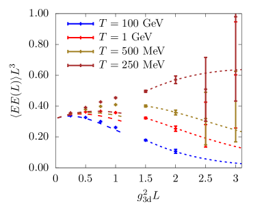
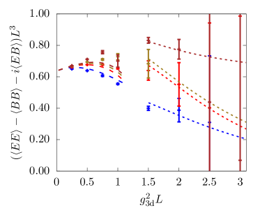
Figure 6.4: Continuum-extrapolated EQCD lattice data on $\langle EE\rangle$ (left) and $\langle FF\rangle$ (right). Short dashes represent the long $L$-tail whole short dashes denote the NLO pEQCD evaluation. $L^{3}$ compensates the $c_{0}/L^{3}$ divergence. Figure from [16].

In Fig. 6.4, the lattice EQCD evaluations of $\langle EE\rangle$ (left) and $\langle FF\rangle$ (right) are shown. One cannot integrate up to arbitrarily large values of $L$ on the lattice, which is made apparent by the rather large error bars in that region. This IR region is addressed by a fitting ansatz, intended to reproduce the expected exponential falloff from electrostatic and magnetostatic screening. In the UV, where $m_{D}L\ll 1$, the lattice determination agrees well with the pEQCD determination, as expected. However, as one moves further into the deep UV, the lattice approach becomes impractical due to associated discretisation effects and one must rely on a perturbative evaluation. Such a perturbative evaluation does not, however, come from pEQCD; as an IR EFT of full QCD, EQCD exhibits unphysical behaviour for momenta $k\gg m_{D}$.

Because of the super-renormalisability of EQCD, in the UV, it is natural to expect that

$$\langle FF\rangle_{m_{D}L\ll 1}=\frac{c_{0}}{L^{3}}+\frac{c_{2}g^{2}_{\text{3d}}}{L^{2}}+\frac{c_{4}g^{4}_{\text{3d}}}{L}+...\,.$$ (6.62)

The first and second terms above are divergent when inserted into Eq. (6.61). The former would have come out of the calculation in Sec. 4.4.2 if we had employed a regularisation other than DR. It moreover cancels against a power law divergence coming from the LO calculation. The latter was computed in [16] and, being a logarithmic divergence, does show up in DR.

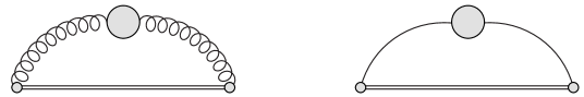
Figure 6.5: EQCD equivalent of diagram $(c)$. The labelling is identical to that from Fig. 6.1 except that here, curly lines represent spatial gauge bosons, solid double lines are (adjoint) Wilson lines and solid lines are adjoint scalars.

To arrive at a solution for $Z_{g}^{\text{3d}}$, accurate across all energy scales, one can imagine stitching the perturbative, intermediate and IR regions together

$$Z_{g}^{\text{3d}}\big{|}^{\text{merge}}= \frac{4T}{d_{A}}\bigg{\{}\int_{0}^{L_{\text{min}}}dL\,L\bigg{[}\langle FF\rangle_{\text{NLO}}-\frac{c_{0}}{L^{3}}-\frac{c_{2}g_{\text{3d}}^{2}}{L^{2}}\bigg{]}+\int_{L_{\text{min}}}^{L_{\text{max}}}dL\,L\bigg{[}\langle FF\rangle_{\text{lat}}-\frac{c_{0}}{L^{3}}\bigg{]}$$

$$\hskip 14.22636pt+\int_{L_{\text{max}}}^{\infty}dL\,L\bigg{[}\langle FF\rangle_{\text{tail}}-\frac{c_{0}}{L^{3}}\bigg{]}\bigg{\}}.$$ (6.63)

$L_{\text{min}}$ is taken to be $0.25/g_{3\text{d}}^{2}$, as can be seen in Fig. 6.4.

Our goal in this section is essentially to check the validity of the NLO subtraction in the first term above. In particular, such a logarithmic UV divergence should cancel against the logarithmic IR divergence from the full QCD calculation that we computed in the previous section. Moreover, from the arguments of Sec. 6.2, we know that this UV divergence must come from the EQCD analogue of diagram $(c)$, shown in Fig. 6.5. We first take the $\langle BB\rangle$ contribution from Appendix A.3 of [16] (Eq. A.14)

$$(c)^{BB}_{\text{div}}=\frac{1}{4}\int_{k}\frac{e^{iLk_{z}}}{k^{4}}(k_{\perp}^{2}+2k_{z}^{2})\delta^{ab}\Big{(}-\Pi^{T}_{A^{a}_{i}A^{b}_{j}\,\text{div}}(k)\Big{)}.$$ (6.64)

where

$$\Pi^{T}_{A^{a}_{i}A^{b}_{j}}(k) =\delta^{ab}\frac{g^{2}_{\text{3d}}C_{A}}{16\pi}\left(-2m_{D}+\frac{14}{4}k+\frac{k^{2}+4m_{D}^{2}}{k}\arctan\frac{k}{2m_{D}}\right)$$

$$\stackrel{{\scriptstyle k\gg m_{D}}}{{\approx}}\delta^{ab}\frac{g^{2}_{3d}C_{A}}{16\pi}\left(-3\pi k\right)\equiv\Pi^{T}_{A^{a}_{i}A^{b}_{j}\,\text{div}}(k).$$ (6.65)

We have expanded for $k\gg m_{D}$ in order to probe its UV, i.e, the region where EQCD is no longer applicable. The loop integration, performed to arrive at Eq. (6.65) was done in $3$ dimensions, whereas the $k$ integration in Eq. (6.64) will be done in $d$ dimensions – this is consistent with the integration procedure followed on the full QCD side. The second term in Eq. (6.65), proportional to $2k_{z}^{2}$ should correspond to the $2k^{-2}$ term computed in Sec. 6.3.1. Indeed, looking to Eq. (6.61), we find

$$Z^{3d\,(c)}_{g\,k^{-2}\,G\,\text{div}} =-\frac{4T}{d_{A}}\int_{0}^{L_{\text{min}}}dL\,L\,(c)^{BB}_{k^{-2}\,\text{div}}$$

$$=\frac{3g^{2}_{3d}C_{A}T}{32\pi^{2}}\Big{(}\frac{1}{\epsilon}-2+3\gamma_{E}+2\ln{L_{\text{min}}\bar{\mu}}+\psi\left(\frac{1}{2}\right)\Big{)}.$$ (6.66)

Given that $g^{2}_{3d}\sim g^{2}T$, it is clear that the $1/\epsilon$ term cancels the one from Eq. (6.49).

As for the $L-T$ piece, we need the contribution from the $\langle EE\rangle$ correlator. Again, we extract this from Eq. A.8 of [16] and expand towards the UV to arrive at

$$\Pi_{\Phi^{a}\Phi^{b}}(k) =\delta^{ab}\frac{g^{2}_{3d}C_{A}m_{D}}{16\pi}\left(-4-\frac{6C_{F}-C_{A}}{6C_{A}}\frac{\lambda_{E}}{g^{2}_{3d}}-8\frac{k^{2}-m_{D}^{2}}{km_{D}}\arctan\frac{k}{m_{D}}\right)$$

$$\stackrel{{\scriptstyle k\gg m_{D}}}{{\approx}}\delta^{ab}\frac{g^{2}_{3d}C_{A}}{16\pi}\left(-4\pi k\right)\equiv\Pi_{\Phi^{a}\Phi^{b}\,\text{div}}(k).$$ (6.67)

From Eq. $A.13$ of [16], we then write

$$(c)^{EE}_{\text{div}}=\frac{1}{4}\int_{k}\frac{e^{iLk_{z}}}{k^{4}}k_{\perp}^{2}\delta^{ab}\Big{(}-\Pi^{T}_{\Phi^{a}\Phi^{b}\,\text{div}}(k)\Big{)}.$$ (6.68)

In order to get the full $\Pi_{L}-\Pi_{T}$ EQCD contribution, we need to add to this the first term in Eq. (6.64), proportional to $k_{\perp}^{2}$. Inserting these into Eq. (6.61),

$$Z^{3d\,(c)}_{g\,L-T\,G\,\text{div}} =-\frac{4T}{d_{A}}\int_{0}^{L_{\text{min}}}dL\,L\,\left((c)^{BB}_{k_{\perp}^{2}\,\text{div}}-(c)^{EE}_{\text{div}}\right)$$

$$=\frac{g^{2}_{3d}C_{A}T}{32\pi^{2}}\bigg{(}\frac{1}{\epsilon}-3+3\gamma_{E}+2\ln{L_{\text{min}}\bar{\mu}}+\psi\left(-\frac{1}{2}\right)\bigg{)},$$ (6.69)

which, reassuringly contains a $1/\epsilon$ pole that cancels exactly against the one from Eq. (6.53). Having confirmed the validity of the subtraction in Eq. (6.63), we proceed to write

$$Z_{g}^{\mathrm{match}}=\frac{g^{2}C_{A}T^{2}}{4\pi^{2}}\bigg{[}\ln(2L_{\text{min}}T)+\gamma_{E}-\frac{3}{2}\bigg{]}\,,\qquad Z_{g}^{\text{non-pert class}}=Z_{g}^{\text{3d}}\big{|}^{\text{merge}}+Z_{g}^{\text{match}},$$ (6.70)

where, from Eqs. (6.49),  (6.53),  (6.66) and  (6.69)

$$Z_{g}^{\text{match}} =Z^{(c)}_{g\,k^{-2}\,G\,n=0}+Z^{\text{3d}\,(c)}_{g\,k^{-2}\,G\,\text{div}}+Z^{(c)}_{g\,L-T\,G\,n=0}+Z^{\text{3d}\,(c)}_{g\,L-T\,G\,\text{div}}$$

$$=\frac{g^{2}C_{A}T^{2}}{8\pi^{2}}\bigg{[}2\ln(2L_{\text{min}}T)+2\gamma_{E}-3\bigg{]}.$$ (6.71)

Note that in computing $Z_{g}^{\text{non-pert class}}$, the $\ln L_{\text{min}}$ above cancels against the $\int dL\frac{c_{2}g_{\text{3d}}^{2}}{L}$ term in Eq. (6.63). For reasonable values of $g_{\text{3d}}$, extracted from [13], we find that $Z_{g}^{\text{non-pert class}}$ provides a negative contribution to $Z_{g}$. However, we should not yet make any conclusive remarks about the convergence of $Z_{g}$ until all of its $\mathcal{O}(g^{2})$ corrections have been obtained. We present the first steps towards a full determination of the $\mathcal{O}(g^{2})$ corrections in the next section.

6.5 Full Evaluation of Diagram $(c)$

We conclude this chapter by completing the evaluation of diagram $(c)$ – the self-energy diagram. The computation is split as follows: the finite-temperature fermionic and gluonic self-energies are given in Secs.6.6,  6.6.1 respectively and the vacuum fermionic and gluonic self-energies are presented together in Sec. 6.6.2. We begin by computing the finite-temperature fermionic contribution, which, naively should be free of any divergences. We discover that such an expectation is not met and comment on sources of these divergences where appropriate. As was done in Sec. 6.3, we further divide up the finite-temperature self-energies into the $k^{-2}$ and $\Pi_{L}-\Pi_{T}$ pieces with the $Q$ integration performed in $4$ dimensions and the $K$ integration in $d$ dimensions. Many of the technical details associated with the integration are left to App. D.3.

6.6 Finite-Temperature Fermionic Contribution

We pick up directly from Eq. (6.9), with the finite-temperature gluon and fermion self-energies given in App. D.2. The contribution from the $k^{-2}$-proportional part is computed in App. D.3.1 and reads

$$Z_{g\,k^{-2}\,F}^{(c)}= \frac{g^{2}T_{F}N_{F}T^{2}}{96\pi^{2}}\bigg{\{}-3\left(4\ln(2)\ln\left(\frac{2}{A^{8}}\right)+2\ln(2)\right)+\frac{\pi^{2}}{6}-8\gamma_{E}\ln 2$$

$$+4.4713-\frac{96\ln 2}{\pi^{2}}+3.7933+1.70118\bigg{\}}.$$ (6.72)

From the absence of any $\epsilon$-dependent terms, it is evidently finite. We have cross-checked this result by numerically performing the sum over the Matusbara modes associated with $K$.

However, we find that the $\text{L}-\text{T}$ contribution, computed in App. D.3.2 is

$$Z_{g\,F\,\text{ L-T }}^{(c)}=\frac{g^{2}T_{F}N_{F}T^{2}}{48\pi^{2}}\bigg{\{}\frac{2}{\epsilon^{2}}+\frac{2\ln\frac{\bar{\mu}\exp(\gamma_{E}+1/2)}{4\pi T}+2(\ln(2)-1)+2\ln\frac{\bar{\mu}A^{12}e^{-1/2}}{16\pi T}}{\epsilon}$$

$$+2\ln^{2}\frac{\bar{\mu}\exp(\gamma_{E}+1/2)}{4\pi T}-4\gamma_{1}+\frac{\pi^{2}}{4}-2\gamma_{E}^{2}+\frac{3}{2}$$

$$+2(\ln(2)-1)\bigg{[}2\ln\frac{\bar{\mu}\exp(\gamma_{E}+1/2)}{4\pi T}\bigg{]}$$

$$+2\ln^{2}\frac{\bar{\mu}A^{12}e^{-1/2}}{16\pi T}$$

$$+48\ln(A)(\gamma_{E}+\ln(2\pi)-6\ln(A))+\frac{12\zeta^{\prime\prime}(2)}{\pi^{2}}+\frac{1}{2}\text{Li}_{2}\left(\frac{2}{3}\right)+\frac{1}{4}\text{Li}_{2}\left(\frac{3}{4}\right)$$

$$-\frac{1}{2}-\frac{11}{2}\ln^{2}(2)-2\ln(\pi)\ln(4\pi)-2\gamma_{E}\left(\gamma_{E}+\ln\left(4\pi^{2}\right)\right)-\frac{1}{2}\ln(3)\coth^{-1}(7)$$

$$\underbrace{-0.438129}_{k<2q}+\underbrace{1.97382}_{k>2q}\bigg{\}}.$$ (6.73)

In contrast to the $k^{-2}$ piece, this contribution is divergent – the $1/\epsilon^{2}$ pole signals the presence of a double logarithmic divergence. We can understand that one of these divergences coming from the region where $k>2q$, implying it is of a UV nature. From only the expression given above, the origin of the other logarithmic divergence is not at all apparent. However, by looking to, for instance, Eq. (D.53), we note the potential for a logarithmic divergence in $k$ when $k^{0}-k\ll k^{0}+k$. This is precisely the region of phase space that is sensitive to collinear physics, where $K^{\mu}\sim T$ with $K^{2}$ small. We thus identify the second logarithmic as a collinear one. We further take this opportunity to hammer home the point that these divergences are not cancelled by opposing ones coming from the soft sector, as EQCD is a theory of gluons only.

6.6.1 Finite-Temperature Gluonic Contribution

We start with the finite-temperature gluonic $k^{-2}$-proportional part, with the details left to App. D.3.3. In this case, we must be mindful not to double count the zero mode contribution already obtained in Eq. (6.49). In doing so, we identify a finite contribution that comes from the non-zero Matsubara modes

$$Z^{(c)}_{g\,k^{-2}\,G\,n\neq 0\,\text{finite}}=-\frac{g^{2}C_{A}T^{2}}{32\pi^{2}}\times 0.00380658,$$ (6.74)

which we have obtained numerically. In addition, we isolate a divergent contribution from the non-zero Matsubara modes, given by

$$Z^{(c)}_{g\,k^{-2}\,G\,n\neq 0\,\text{div}} =\frac{g^{2}C_{A}T^{2}}{48\pi^{2}}\left(\frac{1}{\epsilon}-2\ln\frac{4\pi T}{A^{12}\bar{\mu}}-2.44147-2.44091\right).$$ (6.75)

Unlike the finite-temperature fermionic $k^{-2}$ piece, the gluonic part is divergent – one from the zero-mode and another from the non-zero modes. While we have already discussed the former at length, the latter is of UV nature and we comment further on how it is dealt with at the end of Sec. 6.6.2.

A similar computation, contained in App. D.3.4 shows that the finite-temperature gluonic $\text{L}-\text{T}$ reads

$$Z_{g\,\text{G L-T }}^{(c)}=\frac{g^{2}C_{A}T^{2}}{48\pi^{2}}\bigg{\{}\frac{2}{\epsilon^{2}}+\frac{2\ln\frac{\bar{\mu}\exp(\gamma_{E}+1/2)}{4\pi T}+2(\ln(2)-1)+2\ln\frac{\bar{\mu}A^{12}e^{-1/2}}{8\pi T}}{\epsilon}$$

$$+2\ln^{2}\frac{\bar{\mu}\exp(\gamma_{E}+1/2)}{4\pi T}-4\gamma_{1}+\frac{\pi^{2}}{4}-2\gamma_{E}^{2}+\frac{3}{2}$$

$$+2(\ln(2)-1)\bigg{[}2\ln\frac{\bar{\mu}\exp(\gamma_{E}+1/2)}{4\pi T}\bigg{]}$$

$$+2\ln^{2}\frac{\bar{\mu}A^{12}e^{-1/2}}{8\pi T}$$

$$+48\ln(A)(\gamma_{E}+\ln(2\pi)-6\ln(A))+\frac{12\zeta^{\prime\prime}(2)}{\pi^{2}}+\frac{1}{2}\text{Li}_{2}\left(\frac{2}{3}\right)+\frac{1}{4}\text{Li}_{2}\left(\frac{3}{4}\right)$$

$$-\frac{1}{2}-\frac{3}{2}\ln^{2}(2)-2\ln(\pi)\ln(4\pi)-2\gamma_{E}\left(\gamma_{E}+\ln\left(4\pi^{2}\right)\right)-\frac{1}{2}\ln(3)\coth^{-1}(7)$$

$$+\underbrace{0.145277}_{k<2q}\underbrace{-5.13832}_{k>2q}\bigg{\}}.$$ (6.76)

As was the case in Eq. (6.73), there is a $1/\epsilon^{2}$ pole; by adding Eq. (6.73) and Eq. (6.76) we find the divergent terms are proportional to $m_{D}^{2}$, signifying that the divergences present in both contributions have the same origin.

6.6.2 Vacuum Contribution

Another piece, which was not needed in the matching calculation is given by the vacuum self-energy inserted between the two thermal propagators. The vacuum self-energy (composed of both the fermionic and gluonic pieces) is given in Eq. (D.19). Upon plugging it into Eq. (6.9), we find

$$Z_{g\text{ vac}}^{(c)}=i\frac{\alpha_{s}}{2\pi}\int_{K}[1+n_{\mathrm{B}}(k^{0})]\bigg{[}\frac{-\ln\frac{k^{2}-(k^{0}+i\varepsilon)^{2}}{\bar{\mu}^{2}}\bigg{(}\frac{5}{3}C_{A}-\frac{4}{3}T_{F}N_{F}\bigg{)}+\frac{31}{9}C_{A}-\frac{20}{9}T_{F}N_{F}}{(K^{2}+i\varepsilon k^{0})}-\text{adv}\bigg{]}.$$ (6.77)

To proceed, we rewrite the frequency integration as a Matsubara sum, i.e

$$Z_{g\text{ vac}}^{(c)}=T\sum_{n}\frac{\alpha_{s}}{2\pi}\int_{k}\frac{-\ln\frac{k^{2}+\omega_{n}^{2}}{\bar{\mu}^{2}}\bigg{(}\frac{5}{3}C_{A}-\frac{4}{3}T_{F}N_{F}\bigg{)}+\frac{31}{9}C_{A}-\frac{20}{9}T_{F}N_{F}}{k^{2}+\omega_{n}^{2}}.$$ (6.78)

This yields

$$Z_{g\text{ vac}}^{(c)}= \frac{g^{2}C_{A}T^{2}}{864\pi^{2}}\bigg{[}30\ln\frac{A^{12}\bar{\mu}}{4\pi T}+31\bigg{]}-\frac{g^{2}T_{F}N_{F}T^{2}}{216\pi^{2}}\bigg{[}6\ln\frac{A^{12}\bar{\mu}}{4\pi T}+5\bigg{]}$$

$$= \frac{g^{2}T^{2}}{48\pi^{2}}\bigg{[}\bigg{(}\frac{5}{3}C_{A}-\frac{4}{3}T_{F}N_{F}\bigg{)}\ln\frac{A^{12}\bar{\mu}}{4\pi T}+\frac{31}{18}C_{A}-\frac{10}{9}T_{F}N_{F}\bigg{]}.$$ (6.79)

It is finite as the $\overline{MS}$ subtraction has already been performed in Eq. (6.77). If we instead keep the $1/\epsilon$ poles in Eq. (D.18), we find

$$Z_{g\text{ vac pole}}^{(c)}=T\sum_{n}\frac{\alpha_{s}}{2\pi}\int_{k}\frac{\frac{1}{\epsilon}\bigg{(}\frac{5}{3}C_{A}-\frac{4}{3}T_{F}N_{F}\bigg{)}}{k^{2}+\omega_{n}^{2}}=\frac{g^{2}T^{2}}{96\pi^{2}\epsilon}\bigg{(}\frac{5}{3}C_{A}-\frac{4}{3}T_{F}N_{F}\bigg{)}.$$ (6.80)

Upon adding this to Eq. (6.75), we see that they match the $\beta$ function $C_{A},\,T_{F}N_{F}$ coefficients in (2.13). We therefore understand that these UV divergences are taken care of by the usual UV zero-temperature renormalisation procedure.

6.7 Recap and Discussion of Divergences

With that, we conclude our evaluation of diagram $(c)$ and therefore the $\mathcal{O}(g^{2})$ corrections to $Z_{g}$. Let us briefly lay out our findings:

• In Sec. 6.3, we extracted $Z_{g}$’s (IR) zero-mode divergences. These divergences are expected and are in fact needed as they cancel against UV divergences coming from EQCD at NLO, as we showed in Sec. 6.4. This is one of the main results of the chapter.

• We also identified what we call UV, vacuum divergences coming from Eqs. (6.75), (6.80). We have confirmed that these are subtracted off in the zero-temperature renormalisation.

• Lastly, we have found double-logarithmic UV, collinear divergences, contributing to both the gluonic and fermionic $\text{L}-\text{T}$ pieces in Eqs. (6.73) and (6.76). In contrast to what has been discussed above, these divergences signify that our treatment here is incomplete. As they come from a region of phase space where collinear physics dominates, it is likely that some form of LPM resummation will be needed to cure these divergences. Further investigation on this matter is underway.

As a closing remark, we emphasise that, without a full determination of the $\mathcal{O}(g^{2})$ corrections to $Z_{g}$, the arbitrariness of how the classical corrections are separated from the quantum, $\mathcal{O}(g^{2})$ corrections prevents us from making concrete inferences regarding the numerical size of the non-perturbative evaluation and furthermore, the convergence of the perturbative expansion for $Z_{g}$.

Chapter 7 Conclusion and Outlook

A common theme that has permeated throughout this thesis is the computation of higher-order corrections to $\hat{q}$ and $m_{\infty}$, both of which serve as central inputs to jet energy loss calculations. In particular, the advancements contained in this work are tied to the exploration of quantum corrections at $\mathcal{O}(g^{2})$ to these quantities and how they are related to classical corrections, present at $\mathcal{O}(g)$.

In Ch. 5, we calculated double-logarithmic corrections to $\hat{q}$ in the setting of a weakly coupled QGP. We investigated the consequences of taking the thermal scale seriously in this context and provided clarification, previously lacking in the literature, on how the logarithmically enhanced region of phase space is connected to the classical one. Additionally, we were able to show how the inclusion of semi-collinear processes allows one to go beyond the instantaneous approximation made in the original works [1, 2].

Our result for $\delta\hat{q}(\mu_{\perp})$ at leading double logarithmic accuracy is given by Eq. (5.43) and was obtained in the harmonic oscillator approximation. The necessity of implementing this approximation comes from the need to neglect a neighbouring region of phase space, where both single and multiple scattering can occur; a concrete understanding of this region is lacking in the sense that we do not know the form of the transverse scattering kernel there. In the future, we hope that this issue can be addressed by solving Eq. (5.75). While solving this equation exactly would likely prove to be a formidable task, a first step could be to solve it approximately by using the improved opacity expansion [190, 195, 196, 197]. This could also serve to provide a more satisfying cutoff for the single-scattering regime in the direction of multiple scattering – boundary $(b)$.

We are eager to perform a similar computation and analysis of the single logarithmic corrections to $\hat{q}$. Indeed, next to leading logarithm corrections are often needed to fairly assess the quantitative impact of their leading logarithm counterparts – see [161] for the collinear splitting rate and [124] for QGP transport coefficients. Nevertheless, it does not make sense to move forward in this direction until all of the double logarithmic corrections have been computed.

We could also imagine applying what we have learned to some of the recent developments in jet energy loss theory, mentioned in Sec. 3.7. In more detail, it would be interesting to investigate the impact of the thermal scale in the context of double gluon emission [165, 207, 208, 209, 210, 211, 212, 213, 214, 215, 216, 217], given that the same universal double logarithms also arise in that context.

Another fruitful direction could be to study the resummation of these logarithmic corrections, similarly to what was done in [220, 221, 222, 223]. These authors have performed a resummation according to original triangle shown in Fig. 5.3, evolving $\hat{q}$ from some initial timescale $\tau_{0}$ to longer timescales by resumming longer-lived quantum fluctuations. Our evaluation of the $k^{+}\sim T$ and smaller $\tau$ regions could then be incorporated by evolving $\hat{q}$ through these regions, with the result then being passed on as an initial condition to the resummation equations given in [222, 223].

In Ch. 6, we set out to complete the evaluation of $\mathcal{O}(g^{2})$ corrections to $Z_{g}$ by computing the contribution from the thermal scale. We were able to show that the unphysical UV EQCD divergences, identified in [16], cancel against IR divergences on the full QCD side, thereby providing a finite result to the non-perturbative evaluation of the classical corrections, also calculated in [16]. When computing the rest of the corrections at $\mathcal{O}(g^{2})$, we encountered two other kinds of divergences. The first kind comes from both the fermion and gluon vacuum contribution as well as the $k^{-2}$ finite-temperature gluonic piece. These are UV, vacuum divergences and are appropriately dealt with through the renormalisation of the zero-temperature theory.

The set of divergences, present in both the finite-temperature gluonic and fermionic “$\text{L}-\text{T}$” pieces are more troublesome. They have a collinear origin, i.e, they come from a region of phase space where $K^{\mu}\sim T$ but with $K^{2}$ much smaller. The next course of action in this project is to correctly treat the region from which they emerge, which will likely involve having to take LPM resummation into account. Following this, we plan to compute the $\mathcal{O}(g^{2})$ corrections to $Z_{f}$, which will complete the $\mathcal{O}(g^{2})$ determination of the asymptotic masses. Since $Z_{f}$ is not as sensitive to classical corrections, this should be, in principle, a more straightforward task.

With all of the $\mathcal{O}(g^{2})$ to $\hat{q}$ and $m_{\infty}$ in hand, a more long-term goal would be to assess the quantitative impact of these corrections on the in-medium splitting rate, as was done for the classical corrections to $\hat{q}$ in [13, 14]. This would then pave the way for more phenomenologically-based studies [301, 302], which we originally motivated the need for in the Introduction.

Appendix A Conventions

We take here a moment to specify our notation, which is intended to be particularly suited for studying jet energy loss. We adopt the use of natural units ($\hbar=c=k_{B}=1$) and work in the mostly minus metric, $(+,-,-,-)$.

We write four-momentums with capital letters, $Q=(p^{0},\vec{\mathbf{q}})$, the modulus of three-momentums with lower case letters, $q$ and the modulus of transverse vectors as $q_{\perp}$. Position vectors are denoted similarly. It will often be convenient to use light-cone coordinates such that $Q=(q^{+},q^{-},\mathbf{q})$ with the following convention

$$q^{+} \equiv\frac{q^{0}+q^{z}}{2}=\bar{v}_{\mu}q^{\mu},$$

$$q^{-} \equiv q^{0}-q^{z}=v_{\mu}q^{\mu},$$

$$q\cdot k =q^{+}k^{-}+q^{-}k^{+}-\mathbf{q}\cdot\mathbf{k},$$

where we have defined the two light-like reference vectors as

$$\bar{v}^{\mu} \equiv\frac{1}{2}(1,0,0,-1),$$

$$v^{\mu} \equiv(1,0,0,1).$$

We shall often deal with scalings where $q^{-}\ll q^{+}$, which then implies $q^{0}\approx q^{z}\approx q^{+}$. For the sake of brevity, we introduce the following shorthand for integration over position and momenta in various dimensions

$$\int_{Q} \equiv\int\frac{d^{4}Q}{(2\pi)^{4}}$$

$$\int_{q} \equiv\int\frac{d^{3}q}{(2\pi)^{3}}$$

$$\int_{\mathbf{q}} \equiv\int\frac{d^{2}q_{\perp}}{(2\pi)^{2}}$$

$$\int_{\mathbf{x}} \equiv\int d^{2}x_{\perp}$$

Our convention for the covariant derivative is consistent with that of Schwartz [23]

$$D_{\mu}=\partial_{\mu}-igA_{\mu},$$ (A.1)

which in turn fixes the three-gluon vertex to be

$$\vbox{\hbox{\includegraphics[width=99.58464pt,height=85.35826pt]{three_gluon.pdf}}}\qquad\qquad\begin{aligned} =gf^{abc}V^{\mu\nu\rho},\end{aligned}$$ (A.2)

where

$$V^{\mu\nu\rho}=\eta^{\mu\nu}(K-P)^{\rho}+\eta^{\nu\rho}(P-Q)^{\mu}+\eta^{\rho\mu}(Q-K)^{\nu}.$$ (A.3)

Finallly, we mention our convention for dimensional regularisation

$$\int_{q}=\Big{(}\frac{\bar{\mu}^{2}e^{\gamma_{E}}}{4\pi}\Big{)}^{\epsilon}\int\frac{d^{d}q}{(2\pi)^{d}},$$ (A.4)

where we will often regularise integrals in $d=3-2\epsilon$ dimensions.

Appendix B Wilson Line Details

A Wilson line is a bi-local field that in general depends on two spacetime points

$$\mathcal{V}(Y,Z)=\mathcal{P}\exp\Big(ig\int_{s_{Y}}^{s_{Z}}ds\frac{dX^{\mu}}{ds}A_{\mu}(X(s))\Big{missing}),$$ (B.1)

where $A_{\mu}=A_{\mu}^{a}T^{a}$ is a (non-abelian) Lie-algebra-valued gauge (gluon) field and $\mathcal{P}$ is the path-ordering operator. $\mathcal{P}$ ensures that fields evaluated earlier on the path from $Y$ to $Z$ are placed to the right with respect to fields that are evaluated later on the path. As well as transforming covariantly under gauge transformation, they naturally incorporate the resummation of gluons. We can expand the expression above by first writing

$$\mathbf{\mathcal{F}}(s)=\frac{dX^{\mu}}{ds}A_{\mu},$$ (B.2)

where the bold font is meant to emphasis that these objects are matrices. Then, incorporating the usual definition of the matrix exponential expansion

$$\mathcal{V}(Y,Z)=\sum_{n=0}^{\infty}\left(\frac{ig}{n!}\right)^{n}\int_{s_{Y}}^{s_{Z}}ds_{1}\int_{s_{Y}}^{s_{Z}}ds_{2}...\int_{s_{Y}}^{s_{Z}}ds_{n}\mathcal{P}\Big{[}\mathbf{\mathcal{F}}(s_{1})\mathbf{\mathcal{F}}(s_{2})...\mathbf{\mathcal{F}}(s_{n})\Big{]}$$ (B.3)

The above integration is done over an $n$-dimensional hypercube but one can divide this region into $n!$ sub-regions. To give an illustrative example, consider $n=2,\,s_{Y}=0,\,s_{Z}=1$

$$\int_{0}^{1}ds_{1}\int_{0}^{1}ds_{2}\mathcal{P}\Big{[}\mathbf{\mathcal{F}}(s_{1})\mathbf{\mathcal{F}}(s_{2})\Big{]}=\int_{0}^{1}ds_{1}\int_{0}^{s_{1}}ds_{2}\mathbf{\mathcal{F}}(s_{1})\mathbf{\mathcal{F}}(s_{2})+\int_{0}^{1}ds_{2}\int_{0}^{s_{2}}ds_{1}\mathbf{\mathcal{F}}(s_{2})\mathbf{\mathcal{F}}(s_{1}).$$ (B.4)

At this point, $s_{1},\,s_{2}$ are just dummy variables, so we can write

$$\int_{0}^{1}ds_{1}\int_{0}^{1}ds_{2}\mathcal{P}\Big{[}\mathbf{\mathcal{F}}(s_{1})\mathbf{\mathcal{F}}(s_{2})\Big{]}=2\int_{0}^{1}ds_{1}\int_{0}^{s_{1}}ds_{2}\mathbf{\mathcal{F}}(s_{1})\mathbf{\mathcal{F}}(s_{2}),$$ (B.5)

where such a procedure can be suitably generalised to the the $n$-dimensional case. In this way, one can eliminate the path-ordering rewrite Eq. (B.3) as

$$\mathcal{V}(Y,Z)=\sum_{n=0}^{\infty}\left(ig\right)^{n}\int_{s_{Y}}^{s_{Z}}ds_{1}\int_{s_{Y}}^{s_{1}}ds_{2}...\int_{s_{Y}}^{s_{n-1}}ds_{n}\mathbf{\mathcal{F}}(s_{1})\mathbf{\mathcal{F}}(s_{2})...\mathbf{\mathcal{F}}(s_{n}).$$ (B.6)

In practice, it is this formula that we make use of to calculate Wilson lines in this thesis.

Furthermore, let $s_{Y}=s_{0},\,s_{Z}=s$ so that $Y=X(s_{0})\,Z=X(s)$. Then, by taking a derivative with respect to $s$

$$\frac{dx^{\mu}}{ds}\mathcal{V}(x(s),x(s_{0}))=ig\frac{dx^{\mu}}{ds}A_{\mu}(x(s))\mathcal{V}(x(s),x(s_{0})),$$ (B.7)

we can derive an equation of motion for the Wilson line, which reads

$$\frac{dx^{\mu}}{ds}\Big{(}\frac{\partial}{\partial x^{\mu}}-igA_{\mu}(x(s))\Big{)}\mathcal{V}(s,s_{0})=0=\frac{dx^{\mu}}{ds}D_{\mu}\mathcal{V}(s,s_{0}),$$ (B.8)

where we have used the definition of the covariant derivative, Eq. (A.1).

Appendix C $\hat{q}(\mu_{\perp})$ Computation

C.1 Side rails in Coulomb Gauge

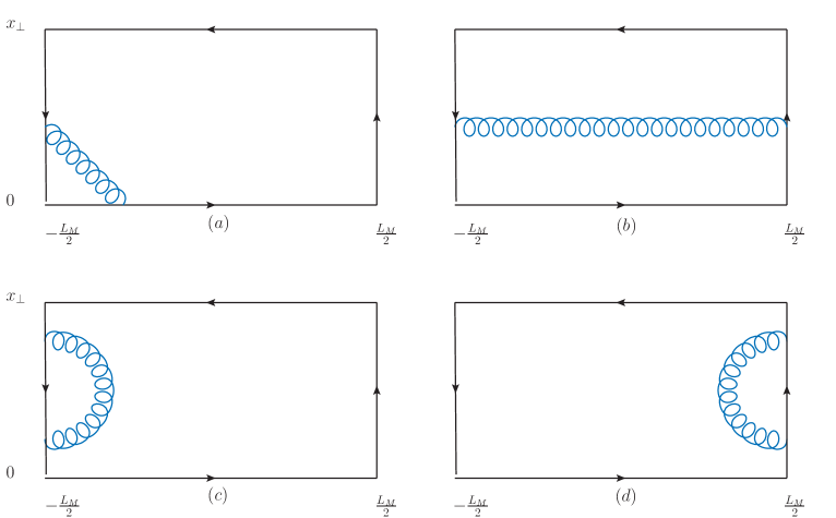
Figure C.1: Diagrams obtained from expanding the Wilson loop to the first non-trivial order, where at least one of the gluon legs are attached to a side rail. In the main text, we argue that none of these diagrams are relevant for the computations performed in this thesis.

Back in Sec. 4.4.1, we showed how to compute the leading order soft contribution to $\hat{q}(\mu_{\perp})$ using the Wilson loop defined in [287]. While carrying out that computation, we only needed to consider the diagrams in Fig. 4.7 where gluons are attached to the horizontal Wilson lines. In this Appendix, we argue why other diagrams, some of which are shown in Fig. C.1 are not relevant for such that calculation, as well as the subsequent ones carried out in Ch. 5.

We start with the top left diagram from Fig. C.1. Using Eqs. (4.91), (4.92), we have

$$(a) =-g^{2}C_{R}\int_{0}^{1}ds\int_{-\frac{L_{M}}{2}}^{\frac{L_{M}}{2}}dx^{+}x_{\perp}\langle G_{>}^{\perp-}(-\frac{L_{M}}{2}-x^{+},0,y_{\perp}s)\rangle$$

$$=-g^{2}C_{R}\int_{0}^{1}ds\int_{-\frac{L_{M}}{2}}^{\frac{L_{M}}{2}}dx^{+}\int_{K}e^{ik^{-}(\frac{L_{M}}{2}+x^{+})}e^{i\mathbf{k}\cdot\mathbf{x}s}x_{\perp}\cdot\langle G_{>}^{\perp-}(K)\rangle,$$ (C.1)

where a sum over the $\perp=x,\,y$ directions is implied. We recognise that $x^{+}$ integration can be rewritten in terms of a delta function, i.e

$$(a)=-g^{2}C_{R}\int_{0}^{1}ds\int_{K}\delta(k^{-})e^{ik^{-}\frac{L_{M}}{2}}e^{i\mathbf{k}\cdot\mathbf{x}s}x_{\perp}\cdot\langle G_{>}^{\perp-}(K)\rangle.$$ (C.2)

Then, upon doing the $k^{-}$ integration, $L_{M}$ will vanish from the entire integrand, implying that this type of diagram will not produce a linear factor of $L_{M}$. Therefore, according to Eq. (4.94), it will furthermore not contribute to $\mathcal{C}(x_{\perp})$.

Moving on to the rest of the diagrams from Fig. C.1, we note that their sum is analogous to the sum of the three diagrams from Fig. 4.7, but in this case with all gluons attached to the side rails

$$\mathcal{C}(x_{\perp})_{\text{side rails}}=-\frac{g^{2}C_{R}}{L_{M}}\int_{1}^{0}ds\int_{1}^{0}dt\int\frac{d^{4}k}{(2\pi)^{4}}e^{-i\mathbf{k}\cdot\mathbf{x}(s+t-1)}(1-e^{-ik^{-}L_{M}})x_{\perp}G^{\perp\perp}_{>}(k)x_{\perp}.$$ (C.3)

The relevant part that we must pay attention to here is

$$\lim_{L_{M}\to\infty}\frac{1}{L_{M}}\int dk^{-}(1-e^{-ik^{-}L_{M}})G^{\perp\perp}_{>}(k).$$ (C.4)

where we have added the limit explicitly because of its particular importance here. For reasons that will soon become clear, it is convenient to divide the integrand by ${k^{-}}^{2}$. Then, by making a change of variable $z=k^{-}L_{M}$ and noting that $G^{\perp\perp}_{>}(z/L_{M})$ is regular as $L_{M}\to\infty$ (in the Coulomb gauge) we can write

$$\lim_{L_{M}\to\infty}\frac{1}{L^{2}}\int dz\frac{1-e^{-iz}}{\frac{z^{2}}{L_{M}^{2}}}G^{\perp\perp}_{rr}(\frac{z}{L_{M}})= \int dz\frac{1-e^{-iz}}{z^{2}}G^{\perp\perp}_{>}(0)$$

$$=G^{\perp\perp}_{>}(0)\int dz\frac{1-\cos(z)}{z^{2}}$$

$$=\pi G^{\perp\perp}_{>}(0)$$ (C.5)

where the final integral over $z$ can be calculated using residue methods. We have just shown that (now it is clear why we divided the integrand by ${k^{-}}^{2}$) Eq. C.4 is indeed proportional to the integral of ${k^{-}}^{2}\delta(k^{-})$, which indeed justifies why we need not worry about these kinds of diagrams, where gluons are attached to the side rails. This clarifies why, throughout the main body of the thesis, the only diagrams that are included are ones where gluons are attached to the horizontal, $\mathcal{W}$ Wilson lines.

C.2 Hard Semi-Collinear Subtraction

In this Appendix, we will show how the second term in Eq. (5.37) is automatically taken into account if we add the hard contribution to $\hat{q}(\mu_{\perp})$ from [174]. Indeed, that paper computes the contribution to $\hat{q}(\mu_{\perp})$ for $\sqrt{ET}\gg k_{\perp}\gg gT$ at leading order, i.e. through elastic Coulomb scatterings with the light quarks and gluons of the medium. The incoming and outgoing momenta for such scatterers are named $P_{2}$ and $P_{2}-Q$ there. We can then identify $P_{2}$ with our $L$ and $Q$ with $-K$. In order to obtain the contribution to $\mathcal{C}(k_{\perp})$ and thence $\hat{q}(\mu_{\perp})$, [174] integrates over all values and orientations of $p_{2}$. In so doing, it ends up including the slice where $p_{2}\sim gT$, $k_{\perp}\sim\sqrt{g}T$, which is precisely the semi-collinear scaling we investigated in Sec. 5.4. As explained there, we need to subtract this limit of [174], so as to avoid double countings.

Our starting point is Eq. (3.8) of [174], where we have specialised to the case of scattering off a soft gluon ($n_{\text{B}}(l^{0})\approx T/l^{0}$) and undone a couple of auxiliary integrals (see (3.7) there), as well as applied the dictionary just described. We then have

$$\delta\mathcal{C}(k_{\perp})^{\text{hard}} =\frac{2g^{4}C_{R}C_{A}}{k_{\perp}^{4}}\int\frac{dk^{0}}{2\pi}\int\frac{dk^{z}}{2\pi}\int\frac{d^{4}L}{(2\pi)^{4}}(l^{0}-l^{z})^{2}\frac{T}{l^{0}}(1+n_{\text{B}}(l^{0}+k^{0}))$$

$$\times 2\pi\delta(k^{0}-k^{z})2\pi\delta((L+K)^{2})2\theta(l^{0}+k^{0})2\theta(l^{0})2\pi\delta(L^{2}).$$ (C.6)

For a soft gluon $L\sim gT$ we can simplify the expression above as

$$\delta\mathcal{C}(k_{\perp})^{\text{hard}} =\frac{2g^{4}C_{R}C_{A}}{k_{\perp}^{4}}\int\frac{dk^{+}}{2\pi}\int\frac{d^{4}L}{(2\pi)^{4}}\frac{Tl^{-2}}{l^{+}+l^{-}/2}(1+n_{\text{B}}(k^{+}))$$

$$\times 2\pi\delta(2k^{+}l^{-}-k_{\perp}^{2})2\theta(k^{+})2\theta(l^{+}+l^{-}/2)2\pi\delta(L^{2}).$$ (C.7)

We can set up the $\delta$ function to fix $l^{+}$, i. e.

$$\delta\mathcal{C}(k_{\perp})^{\text{hard}} =\frac{2g^{4}C_{R}C_{A}}{k_{\perp}^{4}}\int\frac{dk^{+}}{2\pi}\int\frac{d^{4}L}{(2\pi)^{4}}\frac{Tl^{-2}}{l^{+}+l^{-}/2}(1+n_{\text{B}}(k^{+}))\frac{\theta(k^{+})}{k^{+}}$$

$$\times 2\pi\delta\left(l^{-}-\frac{k_{\perp}^{2}}{2k^{+}}\right)\frac{\theta(l^{+}+l^{-}/2)}{\absolutevalue{l^{-}}}2\pi\delta\left(l^{+}-\frac{l_{\perp}^{2}}{2l^{-}}\right).$$ (C.8)

This finally yields

$$\delta\mathcal{C}(k_{\perp})^{\text{hard}}=\frac{g^{2}C_{R}}{\pi k_{\perp}^{4}}\int\frac{dk^{+}}{k^{+}}(1+n_{\text{B}}(k^{+}))\theta(k^{+})\int\frac{d^{2}l_{\perp}}{(2\pi)^{2}}\frac{g^{2}C_{A}T\;2l^{-2}}{l_{\perp}^{2}+l^{-2}}\bigg{|}_{l^{-}=\frac{k_{\perp}^{2}}{2k^{+}}}.$$ (C.9)

It is encouraging to see the resemblance of this result to that of the second term of Eq. (5.37) when plugged in Eq. (5.36). However, to get the two results to match exactly, we need to compute the same result with same integral with instead $L\to L-K$ and $L+K\to L$ keeping $L$ soft, that is, a soft outgoing gluon scatterer. This second integral will give the negative $k^{+}$ contribution, and the integrals’ sum will indeed yield

$$\delta\mathcal{C}(k_{\perp})_{\mathrm{semi}}^{\text{hard}}=\frac{g^{2}C_{R}}{\pi k_{\perp}^{4}}\int\frac{dk^{+}}{k^{+}}(1+n_{\text{B}}(k^{+}))\hat{q}_{\text{\cite[cite]{[\@@bibref{Number}{Arnold:2008vd}{}{}]}}}\left(\rho_{\perp};\frac{k_{\perp}^{2}}{2k^{+}}\right).$$ (C.10)

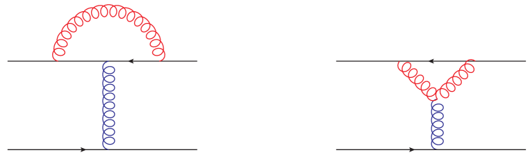
Figure C.2: Diagrams whose cuts correspond to virtual processes.

C.3 Partially Virtual Diagrams

We start from the first diagram in Fig. C.2. As was the case for the real II and X diagrams, the $C_{R}^{2}$-proportional, abelian part of this diagram vanishes with the counterparts, not shown in the figure, where the coft gluon does not straddle the soft one. Accounting for this and for the symmetric diagrams with the coft gluon attached to the other Wilson line we have

$$\delta\mathcal{C}(l_{\perp})^{\mathrm{virt}}_{\widehat{\mathrm{T}}}=-g^{4}C_{R}C_{A}\int\frac{d^{4}K}{(2\pi)^{4}}\int\frac{dl^{+}}{2\pi}\frac{1}{(k^{-}+i\epsilon)^{2}}G_{>}^{--}(L)G_{rr}^{--}(K)\Big{|}_{l^{-}=0},$$ (C.11)

where we have labeled this diagram $\widehat{\mathrm{T}}$ following its topology. We note that the Wilson line integration forces $l^{-}=0$, differently from the real processes. In this case too we defer the evaluation of this expression until after the second diagram has been evaluated. Its contribution, together with that of its symmetric counterpart with two vertices on the bottom Wilson line, is

$$\delta\mathcal{C}(x_{\perp})^{\mathrm{virt}}_{{\mathrm{Y}}}= \frac{g^{4}C_{R}C_{A}}{2}\int\frac{d^{4}K}{(2\pi)^{4}}\int\frac{d^{4}L}{(2\pi)^{4}}\frac{-i}{k^{-}-i\epsilon}e^{i\mathbf{l}\cdot\mathbf{x}}G_{>}^{\beta-}(L)2\pi\delta(l^{-})$$

$$\times\big{(}G_{F}^{-\delta}(K)G_{F}^{-\alpha}(K{+}L)-G_{\bar{F}}^{-\delta}(K)G_{\bar{F}}^{-\alpha}(K{+}L)\big{)}(g_{\delta\beta}(K{-}L)+g_{\beta\alpha}(2L{+}K)_{\delta}-g_{\alpha\delta}(2K{+}L)_{\beta}).$$ (C.12)

We can use the analogue of Eq. (5.10) for the anti-time-ordered propagator, i.e.

$$G_{\bar{F}}(K)=-\frac{1}{2}\Big{(}G_{R}(K)+G_{A}(K)\Big{)}+G_{rr}(K)$$ (C.13)

Using these definitions, we get

$$\delta\mathcal{C}(l_{\perp})^{\mathrm{virt}}_{{\mathrm{Y}}}= g^{4}C_{R}C_{A}\int\frac{d^{4}K}{(2\pi)^{4}}\int\frac{dl^{+}dl^{-}}{2\pi}\frac{i}{k^{-}-i\epsilon}G_{>}^{\beta-}(L)\delta(l^{-})$$

$$\times\big{(}G_{rr}^{-\delta}(K)G_{R}^{-\alpha}(K+L)+G_{R}^{-\delta}(K)G_{rr}^{-\alpha}(K+L)\big{)}(g_{\delta\beta}(K{-}L)+g_{\beta\alpha}(2L{+}K)_{\delta}-g_{\alpha\delta}(2K{+}L)_{\beta}).$$ (C.14)

The virtual contribution is given by the sum of the two, that is

$$\delta\mathcal{C}(l_{\perp})^{\mathrm{virt}}=\delta\mathcal{C}(l_{\perp})^{\mathrm{virt}}_{\widehat{\mathrm{T}}}+\delta\mathcal{C}(l_{\perp})^{\mathrm{virt}}_{{\mathrm{Y}}}.$$ (C.15)

In this case we do not enforce a semi-collinear scaling for the coft gluon, since, as we shall show, there is no double-logarithmic contribution. Furthermore, the Wilson line integrations set $l^{-}=0$, thus making the interaction with the medium instantaneous. We rather assume $l^{+}\sim l_{\perp}\sim k_{\perp}\sim gT\ll k^{+}$, leading to

$$\delta\mathcal{C}(l_{\perp})^{\mathrm{virt}}= 2g^{4}C_{R}C_{A}\int\frac{dl^{+}}{2\pi}\int\frac{dk^{+}d^{2}k_{\perp}}{(2\pi)^{3}}\frac{\frac{1}{2}+n_{\text{B}}(k^{+})}{k^{+}}\frac{G^{--}_{>}(l^{+},l_{\perp})}{k_{\perp}^{2}+m_{\infty\,g}^{2}}$$

$$\times\bigg{[}\frac{k_{\perp}^{2}+\mathbf{k}\cdot\mathbf{l}}{(\mathbf{k}+\mathbf{l})^{2}+m_{\infty\,g}^{2}}-\frac{k_{\perp}^{2}}{k_{\perp}^{2}+m_{\infty g}^{2}}\bigg{]}.$$ (C.16)

The asymptotic masses at the denominator have been included since we assumed $k_{\perp}\sim gT$. They arise from the $k^{+}\sim T$, $K^{2}\sim g^{2}T^{2}$ limit of the HTL propagators in Sec. 4.2.4. The $l^{+}$ integration can be carried out through the mapping to EQCD, as was demonstrated in Sec. 4.4.1. It leads to

$$\delta\mathcal{C}(l_{\perp})^{\mathrm{virt}}= 2g^{4}C_{R}C_{A}\int\frac{dk^{+}d^{2}k_{\perp}}{(2\pi)^{3}}\frac{\frac{1}{2}+n_{\text{B}}(k^{+})}{k^{+}}\frac{Tm_{D}^{2}}{l_{\perp}^{2}(l_{\perp}^{2}+m_{D}^{2})}\frac{1}{k_{\perp}^{2}+m_{\infty\,g}^{2}}$$

$$\times\bigg{[}\frac{k_{\perp}^{2}+\mathbf{k}\cdot\mathbf{l}}{(\mathbf{k}+\mathbf{l})^{2}+m_{\infty\,g}^{2}}-\frac{k_{\perp}^{2}}{k_{\perp}^{2}+m_{\infty\,g}^{2}}\bigg{]}.$$ (C.17)

We recognise that this expression is proportional to the leading-order, adjoint soft scattering kernel $\mathcal{C}(l_{\perp})^{\mathrm{LO}}_{\mathrm{soft}}$, Eq. (3.24). From this expression and its associated $\hat{q}$ contribution one can see that the $|\mathbf{k}+\mathbf{l}|\gg l_{\perp}$ single-scattering region is free of double-logarithmic enhancements, as found in [1]. Furthermore, for $k_{\perp}\sim l_{\perp}\sim gT$, which we have used for our derivation, the lifetime of the virtual coft fluctuation is long, so that multiple soft scatterings can occur within it. Hence, Eq. (C.17) should just be considered as the $\mathcal{N}=1$ term in the opacity expansion of the virtual contribution to Eq. (5.75). Indeed, we have checked that Eq. (C.17) can also be obtained from the virtual terms in Eq. (5.76), i.e. those proportional to $\exp(i\mathbf{x}\cdot\mathbf{l})$, further confirming the soundness of Eqs. (5.73) and (5.75).

Appendix D $Z_{g}$ Computation

This appendix contains some extra details relevant for the calculation in Ch. 6.

D.1 Amputated Self-Energies

It is pointed out in [166] that using KMS relations [263, 264], one can show that amputated self-energies of thermal propagators obey

$$\Pi^{aa}(K) =\left(\frac{1}{2}+n_{\text{B}}(k^{0})\right)\Big{[}\Pi^{R}(K)-\Pi^{A}(K)\Big{]}$$ (D.1)

$$\Pi^{>}(K) =\left(1+n_{\text{B}}(k^{0})\right)\Big{[}\Pi^{R}(K)-\Pi^{A}(K)\Big{]}$$ (D.2)

$$\Pi^{<}(K) =n_{\text{B}}(k^{0})\Big{[}\Pi^{R}(K)-\Pi^{A}(K)\Big{]},$$ (D.3)

where

$$\Pi^{R}(K) =\Pi^{ar}$$ (D.4)

$$\Pi^{A}(K) =\Pi^{ra}.$$ (D.5)

We then define the amputated self-energy-like objects

$$\widetilde{\Pi^{T}}(Q) \equiv G^{F}(K)G^{F}(Q-K),$$ (D.6)

$$\widetilde{\Pi^{<}}(Q) \equiv G^{<}(K)G^{<}(Q-K),$$ (D.7)

$$\widetilde{\Pi^{>}}(Q) \equiv G^{>}(K)G^{>}(Q-K),$$ (D.8)

$$\widetilde{\Pi^{R}}(Q) \equiv G^{rr}(K)G^{R}(Q-K)+G^{rr}(Q-K)G^{R}(K),$$ (D.9)

$$\widetilde{\Pi^{A}}(Q) \equiv G^{rr}(K)G^{A}(Q-K)+G^{rr}(Q-K)G^{A}(K),$$ (D.10)

$$\widetilde{\Pi^{aa}}(Q) \equiv G^{rr}(K)G^{rr}(Q-K)+\frac{1}{4}G^{R}(Q-K)G^{R}(K)+\frac{1}{4}D^{A}(Q-K)D^{A}(K).$$ (D.11)

Strictly speaking, there should be a $K$ integral on the right-hand side of the equations above. However, this would then greatly muddle the notation in and around Eq. (6.18), for instance, where these identities are employed. In the end, it does not matter as we only use these relations to help combine the different assignments; in doing the actual loop integration, we always rewrite everything in terms of the propagators.

D.2 One-Loop Self Energies

In this appendix, we list some finite-temperature one-loop self energies that are needed for the computation in Ch. 6. We essentially copy them from Chapter $8$ of [281] but rewrite them here in such a way that is more suited to our computation.

To start, the gluonic part of the retarded, transverse self-energy reads

$$\Pi_{T}^{R}(K)_{G} =\frac{g^{2}C_{A}}{16\pi^{2}k^{3}}\int_{0}^{\infty}dq\,n_{\mathrm{B}}(q)\bigg{[}8qk\left(k^{2}+k_{0}^{2}\right)$$

$$-K^{2}\left(4q^{2}+4k^{2}+K^{2}\right)\left(\ln\left(\frac{k^{0}+k-2q+i\varepsilon}{k^{0}-k-2q+i\varepsilon}\right)+\ln\left(\frac{k^{0}-k+2q+i\varepsilon}{k^{0}+k+2q+i\varepsilon}\right)\right)$$

$$-4qk^{0}K^{2}\left(2\ln\left(\frac{k^{0}+k+i\varepsilon}{k^{0}-k+i\varepsilon}\right)+\ln\left(\frac{k^{0}-k+2q+i\varepsilon}{k^{0}+k+2q+i\varepsilon}\right)-\ln\left(\frac{k^{0}+k-2q+i\varepsilon}{k^{0}-k-2q+i\varepsilon}\right)\right)\bigg{]}.$$ (D.12)

The finite-temperature, gluonic part of the longitudinal retarded self-energy is instead

$$\Pi_{L}^{R}(K)_{G}= -\frac{g^{2}C_{A}K^{2}}{8\pi^{2}k^{3}}\int_{0}^{\infty}dq\,n_{\mathrm{B}}(q)\bigg{[}8qk$$

$$-\left(4q^{2}-2k^{2}+k_{0}^{2}\right)\bigg{[}\ln\frac{k^{0}+k-2q+i\varepsilon}{k^{0}-k-2q+i\varepsilon}+\ln\frac{k^{0}-k+2q+i\varepsilon}{k^{0}+k+2q+i\varepsilon}\bigg{]}$$

$$-4qk^{0}\bigg{[}2\ln\frac{k^{0}+k+i\varepsilon}{k^{0}-k+i\varepsilon}+\ln\frac{k^{0}-k+2q+i\varepsilon}{k^{0}+k+2q+i\varepsilon}-\ln\frac{k^{0}+k-2q+i\varepsilon}{k^{0}-k-2q+i\varepsilon}\bigg{]}\bigg{]}.$$ (D.13)

It is also worthwhile to have the difference of these two quantities on hand

$$\Pi_{L}^{R}(K)_{G}-\Pi_{T}^{R}(K)_{G}= \frac{g^{2}C_{A}}{16\pi^{2}k^{3}}\int_{0}^{\infty}dq\,n_{\mathrm{B}}(q)\bigg{[}-8qk(3k_{0}^{2}-k^{2})$$

$$+K^{2}\left(12q^{2}-k^{2}+3k_{0}^{2}\right)\bigg{[}\ln\frac{k^{0}+k-2q+i\varepsilon}{k^{0}-k-2q+i\varepsilon}+\ln\frac{k^{0}-k+2q+i\varepsilon}{k^{0}+k+2q+i\varepsilon}\bigg{]}$$

$$+12qk^{0}K^{2}\bigg{[}2\ln\frac{k^{0}+k+i\varepsilon}{k^{0}-k+i\varepsilon}+\ln\frac{k^{0}-k+2q+i\varepsilon}{k^{0}+k+2q+i\varepsilon}-\ln\frac{k^{0}+k-2q+i\varepsilon}{k^{0}-k-2q+i\varepsilon}\bigg{]}.\bigg{]}.$$ (D.14)

The fermionic part of the transverse self-energy is then

$$\Pi^{R}_{T}(K)_{F}= \frac{g^{2}T_{F}N_{F}}{8\pi^{2}k^{3}}\int_{0}^{\infty}dq\,n_{\mathrm{F}}(q)\bigg{[}8qk\left(k^{2}+k_{0}^{2}\right)$$

$$-K^{2}\left(4q^{2}+k^{2}+k_{0}^{2}\right)\bigg{[}\ln\frac{k^{0}+k-2q+i\varepsilon}{k^{0}-k-2q+i\varepsilon}+\ln\frac{k^{0}-k+2q+i\varepsilon}{k^{0}+k+2q+i\varepsilon}\bigg{]}$$

$$-4qk^{0}K^{2}\bigg{[}2\ln\frac{k^{0}+k+i\varepsilon}{k^{0}-k+i\varepsilon}+\ln\frac{k^{0}-k+2q+i\varepsilon}{k^{0}+k+2q+i\varepsilon}-\ln\frac{k^{0}+k-2q+i\varepsilon}{k^{0}-k-2q+i\varepsilon}\bigg{]}\bigg{]}.$$ (D.15)

The longitudinal counterpart is instead

$$\Pi_{L}^{R}(K)_{F}= -\frac{g^{2}T_{F}N_{F}K^{2}}{4\pi^{2}k^{3}}\int_{0}^{\infty}dq\,n_{\mathrm{F}}(q)\bigg{[}8qk$$

$$-\left(4q^{2}-k^{2}+k_{0}^{2}\right)\bigg{[}\ln\frac{k^{0}+k-2q+i\varepsilon}{k^{0}-k-2q+i\varepsilon}+\ln\frac{k^{0}-k+2q+i\varepsilon}{k^{0}+k+2q+i\varepsilon}\bigg{]}$$

$$-4qk^{0}\bigg{[}2\ln\frac{k^{0}+k+i\varepsilon}{k^{0}-k+i\varepsilon}+\ln\frac{k^{0}-k+2q+i\varepsilon}{k^{0}+k+2q+i\varepsilon}-\ln\frac{k^{0}+k-2q+i\varepsilon}{k^{0}-k-2q+i\varepsilon}\bigg{]}\bigg{]},$$ (D.16)

For further use we then have

$$\Pi_{L}^{R}(K)_{F}-\Pi_{T}^{R}(K)_{F}= \frac{g^{2}T_{F}N_{F}}{8\pi^{2}k^{3}}\int_{0}^{\infty}dq\,n_{\mathrm{F}}(q)\bigg{[}-8qk(3k_{0}^{2}-k^{2})$$

$$+K^{2}\left(12q^{2}-k^{2}+3k_{0}^{2}\right)\bigg{[}\ln\frac{k^{0}+k-2q+i\varepsilon}{k^{0}-k-2q+i\varepsilon}+\ln\frac{k^{0}-k+2q+i\varepsilon}{k^{0}+k+2q+i\varepsilon}\bigg{]}$$

$$+12qk^{0}K^{2}\bigg{[}2\ln\frac{k^{0}+k+i\varepsilon}{k^{0}-k+i\varepsilon}+\ln\frac{k^{0}-k+2q+i\varepsilon}{k^{0}+k+2q+i\varepsilon}-\ln\frac{k^{0}+k-2q+i\varepsilon}{k^{0}-k-2q+i\varepsilon}\bigg{]}\bigg{]},$$ (D.17)

We additionally need the vacuum part of the self-energy: The bare vacuum part is [21]

$$\Pi_{L}^{R}(K)_{\text{vac}}=\Pi_{T}^{R}(K)_{\text{vac}}=\frac{\alpha_{s}}{4\pi}K^{2}\bigg{[}\bigg{(}\frac{1}{\epsilon}-\gamma_{E}+\ln(4\pi)-\ln(-K^{2})\bigg{)}\bigg{(}\frac{5}{3}C_{A}-\frac{4}{3}T_{F}N_{F}\bigg{)}+\frac{31}{9}C_{A}-\frac{20}{9}T_{F}N_{F}\bigg{]}.$$ (D.18)

Whereas in the $\overline{MS}$ scheme we have

$$\Pi_{L}^{R}(K)_{\text{vac}\,\overline{MS}}=\Pi_{T}^{R}(K)_{\text{vac}\,\overline{MS}}=\frac{\alpha_{s}}{4\pi}K^{2}\bigg{[}-\ln\frac{k^{2}-(k^{0}+i\varepsilon)^{2}}{\bar{\mu}^{2}}\bigg{(}\frac{5}{3}C_{A}-\frac{4}{3}T_{F}N_{F}\bigg{)}+\frac{31}{9}C_{A}-\frac{20}{9}T_{F}N_{F}\bigg{]}.$$ (D.19)

D.3 Details on Diagram $(c)$ Evaluation

We pack many of the technical details related to the computation in Sec. 6.5 into this appendix.

D.3.1 Fermionic Contribution: $k^{-2}$ Piece

Looking to Eq. (D.15), we start with the simplest terms, i.e. those that do not multiply any log, i.e.

$$\Pi^{R}_{T}(K)_{F\,\text{no log}}= \frac{g^{2}}{16\pi^{2}k^{3}}\int_{0}^{\infty}dq\bigg{[}2T_{F}N_{F}n_{\text{F}}(q)8qk\left(k^{2}+k_{0}^{2}\right)\bigg{]}=\frac{g^{2}T_{F}N_{F}T^{2}}{12k^{2}}\left(k^{2}+k_{0}^{2}\right),$$ (D.20)

Hence

$$Z_{g\,k^{-2}\,F\,\text{ no log}}^{(c)}=i\frac{g^{2}T_{F}N_{F}T^{2}}{6}\int_{K}\Big{(}1+n_{\mathrm{B}}(k^{0})\Big{)}\bigg{[}\frac{(1+k_{0}^{2}/k^{2})}{(K^{2}+i\varepsilon k^{0})^{2}}-\text{adv.}\bigg{]}.$$ (D.21)

We can do the $k^{0}$ integration using contour methods: since the terms in the square brackets have the desired $\text{ret.}-\text{adv}$ structure, we can close the contour in the upper (lower) half-plane to integrate over the retarded (advanced) piece. We find

$$Z_{g\,k^{-2}\,F\,\text{ no log}}^{(c)}= \frac{g^{2}T_{F}N_{F}T^{2}}{6}\int_{K}\Big{(}\frac{1}{2}+n_{\mathrm{B}}(k^{0})\Big{)}\bigg{[}\frac{i(1+k_{0}^{2}/k^{2})}{(K^{2}+i\varepsilon k^{0})^{2}}-\frac{i(1+k_{0}^{2}/k^{2})}{(K^{2}-i\varepsilon k^{0})^{2}}\bigg{]}$$

$$=-\frac{g^{2}T_{F}N_{F}T^{2}}{6}T\sum_{n}\int_{k}\frac{1-\omega_{n}^{2}/k^{2}}{(-k^{2}-\omega_{n}^{2})^{2}}=\frac{g^{2}T_{F}N_{F}T^{2}}{24\pi^{2}}$$ (D.22)

Note that in going from Eq. (D.21), we have rewritten $\big{(}1+n_{\mathrm{B}}(k^{0})\big{)}\rightarrow\big{(}\frac{1}{2}+n_{\mathrm{B}}(k^{0})\big{)}$, which is allowed, because the vacuum part is scaleless and vanishes in DR anyway. The $1/2$ accompanying the statistical function is inserted, precisely because it is the proper term for analytical continuation, and because $1/2+n_{\mathrm{B}}(k^{0})$ is odd, thus complementing the odd expression in square brackets.

Now we move on to the terms with logarithms, starting with the “HTL log” contribution, which is obtained by expanding for $Q\gg K$ in Eq. (D.15)

$$\Pi^{R}_{T}(K)_{F}\bigg{|}_{\text{HTL log}}= -\frac{g^{2}T_{F}N_{F}}{\pi^{2}k^{3}}\int_{0}^{\infty}dq\,n_{\mathrm{F}}(q)qk^{0}K^{2}\ln\frac{k^{0}+k+i\varepsilon}{k^{0}-k+i\varepsilon}$$

$$= -g^{2}T_{F}N_{F}T^{2}\frac{k^{0}K^{2}}{12k^{3}}\ln\frac{k^{0}+k+i\varepsilon}{k^{0}-k+i\varepsilon}.$$ (D.23)

The contribution from this log to $Z_{g}$ reads

$$Z_{g\,k^{-2}\,F\,\text{ HTL log}}^{(c)}=-i\frac{g^{2}T_{F}N_{F}T^{2}}{6}\int_{K}\Big{(}\frac{1}{2}+n_{\mathrm{B}}(k^{0})\Big{)}\bigg{[}\frac{k^{0}}{k^{3}(K^{2}+i\varepsilon k^{0})}\ln\frac{k^{0}+k+i\varepsilon}{k^{0}-k+i\varepsilon}-\text{adv.}\bigg{]}.$$ (D.24)

The reason this term is dealt with separately is that the strategy of separating out a $\delta(K^{2})$ contribution and a $\Theta$-function contribution from the imaginary part of the log in the retarded-advanced difference would in this case give rise to two contributions that are separately divergent on the light-cone at $K^{2}=0$.

We can proceed by re-introducing the auxiliary angular integral and then using analyticity to get the Matsubara modes, i.e.

$$Z_{g\,k^{-2}\,F\,\text{ HTL log}}^{(c)}= -i\frac{g^{2}T_{F}N_{F}T^{2}}{6}\int_{K}\int_{-1}^{1}dx\,\Big{(}\frac{1}{2}+n_{\mathrm{B}}(k^{0})\Big{)}\bigg{[}\frac{k^{0}}{k^{2}(K^{2}+i\varepsilon k^{0})}\frac{1}{k^{0}-kx+i\varepsilon}-\text{adv.}\bigg{]}$$

$$= \frac{g^{2}T_{F}N_{F}T^{2}}{6}T\sum_{n}\int_{k}\int_{-1}^{1}dx\frac{i\omega_{n}}{k^{2}(-\omega_{n}^{2}-k^{2})}\frac{1}{i\omega_{n}-kx}$$

$$= -\frac{g^{2}T_{F}N_{F}T^{2}}{6}T\sum_{n}\int_{k}\int_{-1}^{1}dx\frac{i\omega_{n}}{k^{2}(\omega_{n}^{2}+k^{2})}\frac{-i\omega_{n}+kx}{\omega_{n}^{2}+k^{2}x^{2}}$$ (D.25)

If we keep the even part only of the integer sum we find

$$Z_{g\,F\,\text{HTL log}}^{(c)}= -\frac{g^{2}T_{F}N_{F}T^{2}}{6}T\sum_{n}\int_{k}\int_{-1}^{1}dx\frac{\omega_{n}^{2}}{k^{2}(\omega_{n}^{2}+k^{2})(\omega_{n}^{2}+k^{2}x^{2})}$$

$$= -\frac{g^{2}T_{F}N_{F}T^{2}}{24\pi^{2}}\bigg{[}\frac{\ln(2)}{\epsilon}+\left(-\ln(4)\ln\left(2\frac{4\pi Te^{-\gamma_{E}}}{\bar{\mu}}\right)+\frac{\pi^{2}}{12}+2\ln^{2}(2)+\ln(4)\right)\bigg{]}.$$ (D.26)

Let us now move on to the other $k^{-2}\Pi^{T}$-proportional terms in the fermion contribution, i.e.

$$Z_{g\,k^{-2}\,F\,\text{ non-HTL }}^{(c)}= \frac{ig^{2}T_{F}N_{F}}{4\pi^{2}}\int_{K}\bigg{\{}\frac{1+n_{\mathrm{B}}(k^{0})}{k^{3}(K^{2}+i\varepsilon k^{0})}\int_{0}^{\infty}dq\,n_{\mathrm{F}}(q)\bigg{[}$$

$$-\left(4q^{2}+k^{2}+k_{0}^{2}\right)\bigg{(}\ln\frac{k^{0}+k-2q+i\varepsilon}{k^{0}-k-2q+i\varepsilon}+\ln\frac{k^{0}-k+2q+i\varepsilon}{k^{0}+k+2q+i\varepsilon}\bigg{)}$$

$$-4qk^{0}\bigg{(}\ln\frac{k^{0}-k+2q+i\varepsilon}{k^{0}+k+2q+i\varepsilon}-\ln\frac{k^{0}+k-2q+i\varepsilon}{k^{0}-k-2q+i\varepsilon}\bigg{)}\bigg{]}-\text{adv.}\bigg{\}}.$$ (D.27)

We can split this into a pole part ($\propto\delta(K^{2})$) and a cut part ($\propto\mathbb{P}1/K^{2}$, with $\mathbb{P}$ the principal value). The former reads

$$Z_{g\,k^{-2}\,F\,\text{pole}}^{(c)}= \frac{g^{2}T_{F}N_{F}}{4\pi^{2}}\int_{K}\frac{\frac{1}{2}+n_{\mathrm{B}}(|k^{0}|)}{k^{3}}2\pi\delta(K^{2})\int_{0}^{\infty}dq\,n_{\mathrm{F}}(q)\bigg{[}$$

$$-\left(4q^{2}+k^{2}+k_{0}^{2}\right)\bigg{(}\ln\left|\frac{k^{0}+k-2q}{k^{0}-k-2q}\right|+\ln\left|\frac{k^{0}-k+2q}{k^{0}+k+2q}\right|\bigg{)}$$

$$-4qk^{0}\bigg{(}\ln\left|\frac{k^{0}-k+2q}{k^{0}+k+2q}\right|-\ln\left|\frac{k^{0}+k-2q}{k^{0}-k-2q}\right|\bigg{)}\bigg{]}.$$ (D.28)

This becomes

$$Z_{gk^{-2}\,F\,\text{pole}}^{(c)}= \frac{g^{2}T_{F}N_{F}}{2\pi^{2}}\int_{k}\frac{\frac{1}{2}+n_{\mathrm{B}}(k)}{k^{4}}\int_{0}^{\infty}dq\,n_{\mathrm{F}}(q)\bigg{[}\left(2q^{2}+k^{2}\right)\ln\frac{k+q}{|k-q|}+2qk\ln\frac{|k^{2}-q^{2}|}{q^{2}}\bigg{]}.$$ (D.29)

Let us split this into regions

$$Z_{gk^{-2}\,F\,\text{pole}}^{(c)}= \frac{g^{2}T_{F}N_{F}}{2\pi^{2}}\int_{0}^{\infty}dq\,n_{\mathrm{F}}(q)\int_{k}\frac{\frac{1}{2}+n_{\mathrm{B}}(k)}{k^{4}}$$

$$\times\bigg{\{}\Theta(q-k)\bigg{[}\left(2q^{2}+k^{2}\right)\ln\frac{q+k}{q-k}+2qk\ln\left(1-\frac{k^{2}}{q^{2}}\right)\mp\frac{4qkT}{k\left(\frac{1}{2}+n_{\mathrm{B}}(k)\right)}\bigg{]}$$

$$+\Theta(k-q)\bigg{[}\left(2q^{2}+k^{2}\right)\ln\frac{k+q}{k-q}+2qk\ln\frac{k^{2}-q^{2}}{q^{2}}\bigg{]}\bigg{\}}.$$ (D.30)

The strategy is as follows: on the second line we have introduced a subtraction term, $-4qk$, which renders the integration IR finite, so that we can do it numerically. We then add back $+4qkT/k\left(\frac{1}{2}+n_{\mathrm{B}}(k)\right)$ and do it in DR. For the third line, we instead do the thermal part numerically and the vacuum part analytically in DR. We then find

$$Z_{gk^{-2}\,F\,\text{pole}}^{(c)}=\frac{g^{2}T_{F}N_{F}T^{2}}{96\pi^{2}}\bigg{[}\underbrace{4.4713}_{q>k\text{ num}}\quad\underbrace{-\frac{96\ln 2}{\pi^{2}}}_{q>k\text{ subtr}}\quad\underbrace{+3.7933}_{k>q\text{ therm.}}$$

$$+\frac{1}{\epsilon^{2}}+\frac{2\ln\frac{\bar{\mu}}{8\pi T}+24\ln A+1}{\epsilon}+(48\ln(A)+2)\ln\frac{\bar{\mu}}{8\pi T}+\frac{12\zeta^{\prime\prime}(2)}{\pi^{2}}+2\ln^{2}\frac{\bar{\mu}}{8\pi T}-\frac{\pi^{2}}{12}$$

$$-2\Big{[}2\gamma_{E}(-12\ln(A)+\ln(2\pi))-12(1+2\ln(2\pi))\ln(A)-1+\gamma_{E}^{2}+\ln(2)(\ln(8)-1)$$

$$+\ln(\pi)\ln(4\pi)\Big{]}\bigg{]}.$$ (D.31)

Here $\ln(A)$ is the logarithm of Glaisher’s constant and the terms on the second, third and and fourth lines come from the DR-evaluated vacuum contribution for $k>q$.

Going back to Eq. (D.27) the cut piece on the other hand reads

$$Z_{gk^{-2}\,F\,\text{cut}}^{(c)}= \frac{g^{2}T_{F}N_{F}}{4\pi^{2}}\int_{K}(2\pi)\mathbb{P}\frac{1+n_{\mathrm{B}}(k^{0})}{k^{3}K^{2}}\int_{0}^{\infty}dq\,n_{\mathrm{F}}(q)\bigg{[}$$

$$-\left(4q^{2}+k^{2}+k_{0}^{2}\right)\bigg{(}\Theta(k^{2}-(2q-k^{0})^{2})-\Theta(k^{2}-(2q+k^{0})^{2})\bigg{)}$$

$$+4qk^{0}\bigg{(}\Theta(k^{2}-(2q+k^{0})^{2})+\Theta(k^{2}-(2q-k^{0})^{2})\bigg{)}\bigg{]}$$

$$= \frac{g^{2}T_{F}N_{F}}{4\pi^{2}}\int_{K}(2\pi)\mathbb{P}\frac{\frac{1}{2}+n_{\mathrm{B}}(k^{0})}{k^{3}K^{2}}\int_{0}^{\infty}dq\,n_{\mathrm{F}}(q)\bigg{[}$$

$$-\Theta(k^{2}-(2q-k^{0})^{2})\left((2q-k^{0})^{2}+k^{2}\right)+\Theta(k^{2}-(2q+k^{0})^{2})\left((2q+k^{0})^{2}+k^{2}\right)\bigg{]}.$$ (D.32)

For the cut piece, the strategy is as follows: we exploit the frequency evenness to restrict the frequency integral to twice the positive range.

For the $n_{\mathrm{B}}(k^{0})$-proportional part we first perform the $k$ integration analytically, using the PV prescription for the $k=k^{0}$ singularities. The $k^{0}$ and $q$ integrals can then be done numerically and are free of IR divergences. The $1/2$-proportional part is carried out by first performing the $k^{0}$ integration, to be then followed by the $k$ and $q$ ones. The $k$ integration is divergent and needs to be regulated appropriately. This then yields

$$Z_{gk^{-2}\,F\,\text{cut}}^{(c)}= \frac{g^{2}T_{F}N_{F}T^{2}}{96\pi^{2}}\bigg{\{}-\frac{1}{\epsilon^{2}}-\frac{2\ln\frac{A^{12}\bar{\mu}}{32\pi T}+1}{\epsilon}-2\ln^{2}\frac{A^{12}\bar{\mu}}{32\pi T}-2\ln\frac{A^{12}\bar{\mu}}{32\pi T}$$

$$-\frac{12\zeta^{\prime\prime}(2)}{\pi^{2}}+\frac{72\zeta^{\prime}(2)^{2}}{\pi^{4}}+\frac{7\pi^{2}}{12}-6+8\ln^{2}2-4\ln 2+1.70118\bigg{\}}.$$ (D.33)

Here all terms come from the $1/2$-proportional vacuum part with the exception of the final term, coming from the numerical integrations. Summing the cut and pole contribution yields

$$Z_{g\,k^{-2}\,F\,\text{ non-HTL}}^{(c)}= \frac{g^{2}T_{F}N_{F}T^{2}}{96\pi^{2}}\bigg{\{}\underbrace{4.4713}_{q>k\text{ num}}\quad\underbrace{-\frac{96\ln 2}{\pi^{2}}}_{q>k\text{ subtr}}\quad\underbrace{+3.7933}_{k>q\text{ therm.}}+1.70118$$

$$+\frac{4\ln 2}{\epsilon}+8\ln 2\ln\frac{A^{12}\bar{\mu}}{8\pi T}+\frac{\pi^{2}}{2}-4+2\ln(2)(1-2\ln 2)\bigg{\}}$$ (D.34)

The total contribution from the $k^{-2}$-proportional part in the fermion contribution is, from Eqs. (D.22),  (D.26), and  (D.34) therefore

$$Z_{g\,k^{-2}\,F}^{(c)}= \frac{g^{2}T_{F}N_{F}T^{2}}{96\pi^{2}}\bigg{\{}-3\left(4\ln(2)\ln\left(\frac{2}{A^{8}}\right)+2\ln(2)\right)+\frac{\pi^{2}}{6}-8\gamma_{E}\ln 2$$

$$+4.4713-\frac{96\ln 2}{\pi^{2}}+3.7933+1.70118\bigg{\}}.$$ (D.35)

We can thus see that the entire $k^{-2}$-proportional contribution is finite. The result has been confirmed, by numerically performing the sum over the Matusbara modes associated with $K$.

D.3.2 Fermionic Contribution: $\Pi_{L}-\Pi_{T}$ Piece

Let us start from the HTL subset of the full contribution

$$Z_{g\,F\,\text{ L-T HTL}}^{(c)}=i\int_{K}\frac{1+n_{\mathrm{B}}(k^{0})}{(k^{-}-i\varepsilon)^{2}}\bigg{[}\frac{k_{\perp}^{2}(\Pi_{L}^{R}(K)-\Pi_{T}^{R}(K))_{\mathrm{HTL}}}{k^{2}(K^{2}+i\varepsilon k^{0})}-\text{adv}\bigg{]}.$$ (D.36)

From Eq. (D.17) we then have

$$\Pi_{L}^{R}(K)_{F\,\mathrm{HTL}}-\Pi_{T}^{R}(K)_{F\,\mathrm{HTL}}= \frac{g^{2}T_{F}N_{F}T^{2}}{12}\bigg{[}-\frac{(6k_{0}^{2}-4k^{2})}{k^{2}}+3\frac{k^{0}K^{2}}{k^{3}}\ln\frac{k^{0}+k+i\varepsilon}{k^{0}-k+i\varepsilon}\bigg{]}.$$ (D.37)

The pole contribution is then

$$Z_{g\,F\,\text{ L-T HTL pole}}^{(c)}=-\frac{g^{2}T_{F}N_{F}T^{2}}{12}\int_{K}\frac{\frac{1}{2}+n_{\mathrm{B}}(|k^{0}|)}{(k^{-}-i\varepsilon)^{2}}\frac{(6k_{0}^{2}-4k^{2})}{k^{2}}\bigg{[}\frac{k_{\perp}^{2}}{k^{2}}2\pi\delta(K^{2})\bigg{]}.$$ (D.38)

The vacuum part is scale-free, so in DR, we have

$$Z_{g\,F\,\text{ L-T HTL pole}}^{(c)}=-\frac{g^{2}T_{F}N_{F}T^{2}}{6}\int_{k}\frac{n_{\mathrm{B}}(k)}{2k}\bigg{[}\frac{1}{(k-k^{z}-i\varepsilon)^{2}}+\frac{1}{(-k-k^{z}-i\varepsilon)^{2}}\bigg{]}\frac{k_{\perp}^{2}}{k^{2}}.$$ (D.39)

We drop the $i\varepsilon$ prescription, because DR can make the $x$ integration convergent in the appropriate number of dimensions, i.e.

$$Z_{g\,F\,\text{ L-T HTL pole}}^{(c)}= -\frac{g^{2}T_{F}N_{F}T^{2}}{6}\Big{(}\frac{\bar{\mu}^{2}e^{\gamma_{E}}}{4\pi}\Big{)}^{\epsilon}\frac{2\pi^{d/2-1/2}}{\Gamma(d/2-1/2)(2\pi)^{d}}\int_{0}^{\infty}dk\,k^{d-4}n_{\mathrm{B}}(k)$$

$$\times\int_{-1}^{1}dx(1-x^{2})^{d/2-3/2}\frac{1+x^{2}}{1-x^{2}}.$$

$$= -\frac{g^{2}T_{F}N_{F}T^{2}}{6}\Big{(}\frac{\bar{\mu}^{2}e^{\gamma_{E}}}{4\pi}\Big{)}^{\epsilon}\frac{2\pi^{d/2-1/2}}{\Gamma(d/2-1/2)(2\pi)^{d}}T^{d-3}\zeta(d-3)\Gamma(d-3)$$

$$\frac{\sqrt{\pi}(d-1)\Gamma\left(\frac{d-3}{2}\right)}{2\Gamma\left(\frac{d}{2}\right)}$$

$$=\frac{g^{2}T_{F}N_{F}T^{2}}{48\pi^{2}}\bigg{[}\frac{1}{\epsilon^{2}}+\frac{2\ln\frac{\bar{\mu}\exp(\gamma_{E}+1/2)}{4\pi T}}{\epsilon}+2\ln^{2}\frac{\bar{\mu}\exp(\gamma_{E}+1/2)}{4\pi T}-4\gamma_{1}+\frac{\pi^{2}}{4}-2\gamma_{E}^{2}+\frac{3}{2}\bigg{]}.$$ (D.40)

The cut contribution of the HTL piece is instead

$$Z_{g\,F\,\text{ L-T HTL cut}}^{(c)}=\frac{g^{2}T_{F}N_{F}T^{2}}{4}\int_{K}\frac{1+n_{\mathrm{B}}(k^{0})}{(k^{-}-i\varepsilon)^{2}}\frac{k_{\perp}^{2}k^{0}}{k^{5}}2\pi\Theta(k^{2}-k_{0}^{2}).$$ (D.41)

To simplify things, let us symmetrise the frequency integration

$$Z_{g\,F\,\text{ L-T HTL cut}}^{(c)}=\frac{g^{2}T_{F}N_{F}T^{2}}{4}\int_{K}\frac{k_{\perp}^{2}k^{0}}{k^{5}}2\pi\Theta(k^{2}-k_{0}^{2})\frac{1}{2}\bigg{[}\frac{1+n_{\mathrm{B}}(k^{0})}{(k^{0}-k^{z}-i\varepsilon)^{2}}-\frac{-n_{\mathrm{B}}(k^{0})}{(-k^{0}-k^{z}-i\varepsilon)^{2}}\bigg{]}.$$ (D.42)

As this integral is now even, we can restrict over twice the positive range, i.e.

$$Z_{g\,F\,\text{ L-T HTL cut}}^{(c)}=\frac{g^{2}T_{F}N_{F}T^{2}}{4}\int_{0}^{\infty}\frac{dk^{0}}{2\pi}\int_{k}\frac{k_{\perp}^{2}k^{0}}{k^{5}}2\pi\Theta(k^{2}-k_{0}^{2})\bigg{[}\frac{1+n_{\mathrm{B}}(k^{0})}{(k^{0}-k^{z}-i\varepsilon)^{2}}+\frac{n_{\mathrm{B}}(k^{0})}{(k^{0}+k^{z}+i\varepsilon)^{2}}\bigg{]}.$$ (D.43)

The $n_{\mathrm{B}}$-independent part is now scale-free, while the rest can be done in a somewhat similar way to the pole piece

$$Z_{g\,F\,\text{ L-T HTL cut}}^{(c)}=\frac{g^{2}T_{F}N_{F}T^{2}}{4}\Big{(}\frac{\bar{\mu}^{2}e^{\gamma_{E}}}{4\pi}\Big{)}^{\epsilon}\frac{2\pi^{d/2-1/2}}{\Gamma(d/2-1/2)(2\pi)^{d-1}}\int_{0}^{\infty}\frac{dk^{0}}{2\pi}k^{0}n_{\mathrm{B}}(k^{0})$$

$$\times\int_{k_{0}}^{\infty}dkk^{d-4}\int_{-1}^{1}dx(1-x^{2})^{d/2-1/2}\bigg{[}\frac{1}{(k^{0}-kx-i\varepsilon)^{2}}+\frac{1}{(k^{0}+kx+i\varepsilon)^{2}}\bigg{]}.$$ (D.44)

Our strategy here is to do the following subtraction: $n_{\mathrm{B}}(k^{0})\to n_{\mathrm{B}}(k^{0})\mp(T/k^{0}-\Theta(T-k^{0})/2)$. In this way, the subtraction is finite, and then we re-evaluate the addition in DR. For the finite part, we can first perform the angular and momentum integration, i.e.

$$Z_{g\,F\,\text{ L-T HTL cut finite}}^{(c)}=\frac{g^{2}T_{F}N_{F}T^{2}}{4}\frac{1}{2\pi}\int_{0}^{\infty}\frac{dk^{0}}{2\pi}k^{0}\bigg{[}n_{\mathrm{B}}(k^{0})-\frac{T}{k^{0}}+\frac{\Theta(T-k^{0})}{2}\bigg{]}$$

$$\times\int_{k^{0}}^{\infty}\frac{dk}{k}\int_{-1}^{1}dx(1-x^{2})\bigg{[}\frac{1}{(k^{0}-kx-i\varepsilon)^{2}}+\frac{1}{(k^{0}+kx+i\varepsilon)^{2}}\bigg{]}$$

$$= \frac{g^{2}T_{F}N_{F}T^{2}}{4}\frac{1}{2\pi}\int_{0}^{\infty}\frac{dk^{0}}{2\pi}k^{0}\bigg{[}n_{\mathrm{B}}(k^{0})-\frac{T}{k^{0}}+\frac{\Theta(T-k^{0})}{2}\bigg{]}$$

$$\times\int_{k^{0}}^{\infty}\frac{dk}{k}\bigg{[}\frac{4k^{0}\tanh^{-1}\left(\frac{2kk^{0}}{k^{2}+k_{0}^{2}}\right)}{k^{3}}-\frac{8}{k^{2}}\bigg{]}$$

$$= \frac{2g^{2}T_{F}N_{F}T^{2}}{3}(\ln 2-1)\frac{1}{(2\pi)^{2}}\int_{0}^{\infty}\frac{dk^{0}}{k^{0}}\bigg{[}n_{\mathrm{B}}(k^{0})-\frac{T}{k^{0}}+\frac{\Theta(T-k^{0})}{2}\bigg{]}$$

$$= \frac{g^{2}T_{F}N_{F}T^{2}}{12\pi^{2}}\ln\frac{T}{\omega_{\text{T}}}(\ln 2-1),$$ (D.45)

where $\omega_{\text{T}}=2\pi T\exp(-\gamma_{E})$. For the DR part subtracted part we can instead do frequency first and forget about the zero-mode subtraction, because it will be scale-free. Then

$$Z_{g\,F\,\text{ L-T HTL cut div}}^{(c)}=-\frac{g^{2}T_{F}N_{F}T^{2}}{4}\Big{(}\frac{\bar{\mu}^{2}e^{\gamma_{E}}}{4\pi}\Big{)}^{\epsilon}\frac{2\pi^{d/2-1/2}}{\Gamma(d/2-1/2)(2\pi)^{d-1}}\int_{0}^{\infty}dkk^{d-4}$$

$$\times\int_{0}^{k}\frac{dk^{0}}{2\pi}k^{0}\frac{\Theta(T-k^{0})}{2}\int_{-1}^{1}dx(1-x^{2})^{d/2-1/2}\bigg{[}\frac{1}{(k^{0}-kx-i\varepsilon)^{2}}+\frac{1}{(k^{0}+kx+i\varepsilon)^{2}}\bigg{]}.$$ (D.46)

We can continue splitting this in the $k>T$ and $k<T$ ranges, i.e.

$$Z_{g\,F\,\text{ L-T HTL cut div}}^{(c)}=-\frac{g^{2}T_{F}N_{F}T^{2}}{8}\Big{(}\frac{\bar{\mu}^{2}e^{\gamma_{E}}}{4\pi}\Big{)}^{\epsilon}\frac{2\pi^{d/2-1/2}}{\Gamma(d/2-1/2)(2\pi)^{d}}$$

$$\times\int_{0}^{\infty}dkk^{d-4}\int_{-1}^{1}dx(1-x^{2})^{d/2-1/2}\bigg{\{}\Theta(T-k)\bigg{[}-\mathbb{P}\frac{2}{1-x^{2}}+\ln\frac{1-x^{2}}{x^{2}}\bigg{]}$$

$$+\Theta(k-T)\bigg{[}\ln\frac{\left|T^{2}-k^{2}x^{2}\right|}{k^{2}x^{2}}-\mathbb{P}\frac{2T^{2}}{T^{2}-k^{2}x^{2}}\bigg{]}\bigg{\}},.$$ (D.47)

where we have used the fact that the imaginary parts of the frequency integral are odd in $x$ and thus vanish. The principal value arises from the $\varepsilon\to 0$ limit. The $k>T$ slice is finite, since the $k$ integration is IR divergent, while the $T>k$ part is IR divergent and needs regularisation. We then have

$$Z_{g\,F\,\text{ L-T HTL cut div}}^{(c)}=-\frac{g^{2}T_{F}N_{F}T^{2}}{8}\Big{(}\frac{\bar{\mu}^{2}e^{\gamma_{E}}}{4\pi}\Big{)}^{\epsilon}\frac{2\pi^{d/2-1/2}}{\Gamma(d/2-1/2)(2\pi)^{d}}$$

$$\times\bigg{\{}\int_{-1}^{1}dx(1-x^{2})^{d/2-1/2}\frac{T^{d-3}}{d-3}\bigg{[}-\mathbb{P}\frac{2}{1-x^{2}}+\ln\frac{1-x^{2}}{x^{2}}\bigg{]}$$

$$+\int_{-1}^{1}dx(1-x^{2})\bigg{[}\frac{\text{Li}_{2}\left(x^{2}\right)}{2}+\ln\left(\frac{x^{2}}{1-x^{2}}\right)+\ln^{2}|x|-\frac{\pi^{2}}{6}\bigg{]}\bigg{\}},$$ (D.48)

which yields

$$Z_{g\,F\,\text{ L-T HTL cut div}}^{(c)}=-\frac{g^{2}T_{F}N_{F}T^{2}}{8}\Big{(}\frac{\bar{\mu}^{2}e^{\gamma_{E}}}{4\pi}\Big{)}^{\epsilon}\frac{2\pi^{d/2-1/2}}{\Gamma(d/2-1/2)(2\pi)^{d}}$$

$$\times\bigg{\{}\frac{T^{d-3}}{d-3}\frac{\sqrt{\pi}\Gamma\left(\frac{d}{2}+\frac{1}{2}\right)\left(\psi^{(0)}\left(\frac{d}{2}-\frac{1}{2}\right)+\gamma-2+2\ln(2)\right)}{\Gamma\left(\frac{d}{2}+1\right)}$$

$$+\frac{1}{9}\left(-8-\pi^{2}+8\ln 2)\right)\bigg{\}}$$

$$= -\frac{g^{2}T_{F}N_{F}T^{2}}{8}\bigg{[}\frac{1-\ln 2}{3\pi^{2}\epsilon}+\frac{(1-\ln 2)(2\ln\frac{\bar{\mu}}{2T}+1)}{3\pi^{2}}\bigg{]},$$ (D.49)

so that finally

$$Z_{g\,F\,\text{ L-T HTL cut}}^{(c)}=\frac{g^{2}T_{F}N_{F}T^{2}}{24\pi^{2}}(\ln(2)-1)\bigg{[}\frac{1}{\epsilon}+2\ln\frac{\bar{\mu}\exp(\gamma_{E}+1/2)}{4\pi T}\bigg{]}.$$ (D.50)

Let us now consider the non-HTL piece, i.e

$$\delta\Pi_{L}^{R}(K)_{F}-\delta\Pi_{T}^{R}(K)_{F}=\frac{g^{2}T_{F}N_{F}K^{2}}{8\pi^{2}k^{3}}\int_{0}^{\infty}dq\,n_{\mathrm{F}}(q)\bigg{[}24qk$$

$$+\left(12q^{2}-k^{2}+3k_{0}^{2}\right)\bigg{[}\ln\frac{k^{0}+k-2q+i\varepsilon}{k^{0}-k-2q+i\varepsilon}+\ln\frac{k^{0}-k+2q+i\varepsilon}{k^{0}+k+2q+i\varepsilon}\bigg{]}$$

$$+12qk^{0}\bigg{[}\ln\frac{k^{0}-k+2q+i\varepsilon}{k^{0}+k+2q+i\varepsilon}-\ln\frac{k^{0}+k-2q+i\varepsilon}{k^{0}-k-2q+i\varepsilon}\bigg{]}\bigg{]},$$ (D.51)

where $\delta\Pi=\Pi-\Pi_{\text{HTL}}$. This then gives

$$Z_{g\,F\,\text{ L-T non-HTL}}^{(c)}=\frac{g^{2}T_{F}N_{F}}{4\pi}\int_{0}^{\infty}dq\,n_{\mathrm{F}}(q)\int_{K}\frac{\frac{1}{2}+n_{\mathrm{B}}(k^{0})}{(k^{-}-i\varepsilon)^{2}}\frac{k_{\perp}^{2}}{k^{5}}$$

$$\times\bigg{[}\Theta(k^{2}-(k^{0}-2q)^{2})\left(3(2q-k^{0})^{2}-k^{2}\right)-\Theta(k^{2}-(k^{0}+2q)^{2})\left(3(2q+k^{0})^{2}-k^{2}\right)\bigg{]}.$$ (D.52)

Here we used the fact that the 1/2 piece vanishes to restrict to the purely odd $1/2+n_{\mathrm{B}}(k^{0})$ component. Let us again symmetrise and restrict to twice the positive frequency range:

$$Z_{g\,F\,\text{ L-T non-HTL}}^{(c)}=\frac{g^{2}T_{F}N_{F}}{4\pi}\int_{0}^{\infty}dq\,n_{\mathrm{F}}(q)\int_{0}^{\infty}\frac{dk^{0}}{2\pi}\int_{k}\frac{k_{\perp}^{2}}{k^{5}}\bigg{[}\frac{\frac{1}{2}+n_{\mathrm{B}}(k^{0})}{(k^{0}-k^{z}-i\varepsilon)^{2}}+\frac{\frac{1}{2}+n_{\mathrm{B}}(k^{0})}{(k^{0}+k^{z}+i\varepsilon)^{2}}\bigg{]}$$

$$\times\bigg{[}\Theta(k^{2}-(k^{0}-2q)^{2})\left(3(2q-k^{0})^{2}-k^{2}\right)-\Theta(k^{2}-(k^{0}+2q)^{2})\left(3(2q+k^{0})^{2}-k^{2}\right)\bigg{]}.$$ (D.53)

This corresponds to

$$Z_{g\,F\,\text{ L-T non-HTL}}^{(c)}=\frac{g^{2}T_{F}N_{F}}{4\pi}\int_{0}^{\infty}dq\,n_{\mathrm{F}}(q)\int_{0}^{\infty}\frac{dk^{0}}{2\pi}\int_{k}\frac{k_{\perp}^{2}}{k^{5}}\bigg{[}\frac{1/2+n_{\mathrm{B}}(k^{0})}{(k^{0}-k^{z}-i\varepsilon)^{2}}+\frac{1/2+n_{\mathrm{B}}(k^{0})}{(k^{0}+k^{z}+i\varepsilon)^{2}}\bigg{]}$$

$$\times\bigg{\{}\Theta(k-2q)\bigg{[}\left(3(2q-k^{0})^{2}-k^{2}\right)\Theta(2q+k-k^{0})-\left(3(2q+k^{0})^{2}-k^{2}\right)\Theta(k-2q-k^{0})\bigg{]}$$

$$+\Theta(2q-k)\left(3(2q-k^{0})^{2}-k^{2}\right)\Theta(2q+k-k^{0}))\Theta(k^{0}+k-2q)\bigg{\}}.$$ (D.54)

We start by dealing with the vacuum part

$$Z_{g\,F\,\text{ L-T non-HTL vac}}^{(c)}=\frac{g^{2}T_{F}N_{F}}{8\pi}\int_{0}^{\infty}dq\,n_{\mathrm{F}}(q)\int_{0}^{\infty}\frac{dk^{0}}{2\pi}\int_{k}\frac{k_{\perp}^{2}}{k^{5}}\bigg{[}\frac{1}{(k^{0}-k^{z}-i\varepsilon)^{2}}+\frac{1}{(k^{0}+k^{z}+i\varepsilon)^{2}}\bigg{]}$$

$$\times\bigg{\{}\Theta(k-2q)\bigg{[}\left(3(2q-k^{0})^{2}-k^{2}\right)\Theta(k+2q-k^{0})-\left(3(2q+k^{0})^{2}-k^{2}\right)\Theta(k-2q-k^{0})\bigg{]}$$

$$+\Theta(2q-k)\left(3(2q-k^{0})^{2}-k^{2}\right)\Theta(2q+k-k^{0})\Theta(k^{0}-2q+k)\bigg{\}},$$ (D.55)

which we can simplify as

$$Z_{g\,F\,\text{ L-T non-HTL vac}}^{(c)}=\frac{g^{2}T_{F}N_{F}}{8\pi}\int_{0}^{\infty}dq\,n_{\mathrm{F}}(q)\int_{0}^{\infty}\frac{dk^{0}}{2\pi}\int_{k}\frac{k_{\perp}^{2}}{k^{5}}\bigg{[}\frac{1}{(k^{0}-k^{z}-i\varepsilon)^{2}}+\frac{1}{(k^{0}+k^{z}+i\varepsilon)^{2}}\bigg{]}$$

$$\times\bigg{\{}\Theta(k-2q)\bigg{[}\left(3(2q-k^{0})^{2}-k^{2}\right)\Theta(k+2q-k^{0})\Theta(k^{0}-k+2q)-24qk^{0}\Theta(k-2q-k^{0})\bigg{]}$$

$$+\Theta(2q-k)\left(3(2q-k^{0})^{2}-k^{2}\right)\Theta(2q+k-k^{0})\Theta(k^{0}-2q+k)\bigg{\}},$$ (D.56)

The strategy here is the following: we further symmetrise the expression in $k^{z}$, to perform the $k^{0}$ integrations. After that one can take $\varepsilon\to 0$. Logarithmic pieces will see their argument change to its absolute value, while possible imaginary parts will cancel out due to $k^{z}$ symmetrisation (in essence, the imaginary part is odd in $k^{z}$ and thus vanishing). Non-logarithmic pieces present poles on the $k^{z}$ integration range. If we restrict to twice the positive $k^{z}$ range, these occur at $-|2q-k|+k^{z}=0$ and are turned into a PV prescription by the $\varepsilon\to 0$ limit. We can thus proceed to the $k^{z}$ integral in the two ranges $2q>k$ and $k>2q$. In the latter case, we find two subranges, one for $k_{\perp}<2q$ and one for $k_{\perp}>2q$. This last one has to be carried out in DR, since it contains a UV divergence. We then find

$$Z_{g\,F\,\text{ L-T non-HTL vac}}=\frac{g^{2}T_{F}N_{F}T^{2}}{48\pi^{2}}\bigg{\{}\frac{1}{\epsilon^{2}}+\frac{2}{\epsilon}\ln\frac{\bar{\mu}A^{12}e^{-1/2}}{16\pi T}+2\ln^{2}\frac{\bar{\mu}A^{12}e^{-1/2}}{16\pi T}$$

$$+48\ln(A)(\gamma_{E}+\ln(2\pi)-6\ln(A))+\frac{12\zeta^{\prime\prime}(2)}{\pi^{2}}+\frac{1}{2}\text{Li}_{2}\left(\frac{2}{3}\right)+\frac{1}{4}\text{Li}_{2}\left(\frac{3}{4}\right)$$

$$-\frac{1}{2}-\frac{11}{2}\ln^{2}(2)-2\ln(\pi)\ln(4\pi)-2\gamma_{E}\left(\gamma_{E}+\ln\left(4\pi^{2}\right)\right)-\frac{1}{2}\ln(3)\coth^{-1}(7)\bigg{\}}.$$ (D.57)

For the thermal part we have instead

$$Z_{g\,F\,\text{ L-T non-HTL th}}^{(c)}=\frac{g^{2}T_{F}N_{F}}{2\pi}\int_{0}^{\infty}dq\,n_{\mathrm{F}}(q)\int_{0}^{\infty}\frac{dk^{0}}{2\pi}\int_{0}^{\infty}\frac{dk}{4\pi^{2}}\frac{n_{\mathrm{B}}(k^{0})}{k}$$

$$\times\bigg{[}\frac{2k^{0}\tanh^{-1}\left(\frac{2kk^{0}}{k^{2}+k_{0}^{2}}\right)}{k^{3}}-\frac{4}{k^{2}}\bigg{]}$$

$$\times\bigg{\{}\Theta(k-2q)\bigg{[}\left(3(2q-k^{0})^{2}-k^{2}\right)\Theta(2q+k-k^{0})-\left(3(2q+k^{0})^{2}-k^{2}\right)\Theta(k-2q-k^{0})\bigg{]}$$

$$+\Theta(2q-k)\left(3(2q-k^{0})^{2}-k^{2}\right)\Theta(2q+k-k^{0}))\Theta(k^{0}+k-2q)\bigg{\}}.$$ (D.58)

Here we instead perform $k$ first analytically, followed by $k^{0}$ and $q$ numerically. We find

$$Z_{g\,F\,\text{ L-T non-HTL th}}^{(c)}=\frac{g^{2}T_{F}N_{F}T^{2}}{48\pi^{2}}\bigg{[}\underbrace{-0.438129}_{k<2q}+\underbrace{1.97382}_{k>2q}\bigg{]}.$$ (D.59)

Putting everything together we find

$$Z_{g\,F\,\text{ L-T }}^{(c)}=\frac{g^{2}T_{F}N_{F}T^{2}}{48\pi^{2}}\bigg{\{}\frac{2}{\epsilon^{2}}+\frac{2\ln\frac{\bar{\mu}\exp(\gamma_{E}+1/2)}{4\pi T}+2(\ln(2)-1)+2\ln\frac{\bar{\mu}A^{12}e^{-1/2}}{16\pi T}}{\epsilon}$$

$$+2\ln^{2}\frac{\bar{\mu}\exp(\gamma_{E}+1/2)}{4\pi T}-4\gamma_{1}+\frac{\pi^{2}}{4}-2\gamma_{E}^{2}+\frac{3}{2}$$

$$+2(\ln(2)-1)\bigg{[}2\ln\frac{\bar{\mu}\exp(\gamma_{E}+1/2)}{4\pi T}\bigg{]}$$

$$+2\ln^{2}\frac{\bar{\mu}A^{12}e^{-1/2}}{16\pi T}$$

$$+48\ln(A)(\gamma_{E}+\ln(2\pi)-6\ln(A))+\frac{12\zeta^{\prime\prime}(2)}{\pi^{2}}+\frac{1}{2}\text{Li}_{2}\left(\frac{2}{3}\right)+\frac{1}{4}\text{Li}_{2}\left(\frac{3}{4}\right)$$

$$-\frac{1}{2}-\frac{11}{2}\ln^{2}(2)-2\ln(\pi)\ln(4\pi)-2\gamma_{E}\left(\gamma_{E}+\ln\left(4\pi^{2}\right)\right)-\frac{1}{2}\ln(3)\coth^{-1}(7)$$

$$\underbrace{-0.438129}_{k<2q}+\underbrace{1.97382}_{k>2q}\bigg{\}}.$$ (D.60)

In contrast to the $k^{-2}$ piece, this contribution is indeed divergent. Moreover, we hammer home the point that these divergences are not cancelled by opposing ones coming from the soft sector, as EQCD is a theory of gluons only.

D.3.3 Gluonic Contribution: $k^{-2}$ Piece

We persevere with the full contribution to diagram $(c)$, starting with the gluonic $k^{-2}$ piece, as we did for the fermionic counterpart in Sec. D.3.1.

Our starting point is Eq. (6.47): we need to be aware that there may be divergences, other than the zero-mode contribution, Eq. (6.49). Upon computing the contribution of the non-zero Matsubara modes numerically, we see a (logarithmic) divergence appearing. In order to isolate the finite contribution, we perform a subtraction on Eq. (6.47) so that we are essentially left with the equivalent fermionic expression (up to the factor of $n_{B}(k)$), which was finite. This leaves us with

$$Z^{(c)}_{g\,k^{-2}\,G\,n\neq 0\,\text{finite}}=-\frac{g^{2}C_{A}T}{8\pi^{2}}\sum_{n\neq 0}\int_{k}\int_{0}^{\infty}dq\frac{1}{k^{3}}n_{\text{B}}(q)\frac{1}{(-\omega_{n}^{2}-k^{2})^{2}}\Bigg{(}8qk(k^{2}-\omega_{n}^{2})$$

$$-(-\omega_{n}^{2}-k^{2})(4q^{2}+k^{2}-\omega_{n}^{2})\left(\ln\frac{i\omega_{n}+k-2q}{i\omega_{n}-k-2q}+\ln\frac{i\omega_{n}-k+2q}{i\omega_{n}+k+2q}\right)$$

$$-4iq\omega_{n}(-\omega_{n}^{2}-k^{2})\left(2\ln\frac{i\omega_{n}+k}{i\omega_{n}-k}+\ln\frac{i\omega_{n}-k+2q}{i\omega_{n}+k+2q}-\ln\frac{i\omega_{n}+k-2q}{i\omega_{n}-k-2q}\right)\Bigg{)}$$

$$=-\frac{g^{2}C_{A}T^{2}}{32\pi^{2}}\times 0.00380658$$ (D.61)

The divergent part then reads

$$Z^{(c)}_{g\,k^{-2}\,G\,n\neq 0\,\text{div}} =-\frac{g^{2}C_{A}T}{4\pi^{2}}\sum_{n\neq 0}\int_{k}\int_{0}^{\infty}dq\frac{n_{B}(q)}{k(\omega_{n}^{2}+k^{2})}\left(\ln\frac{i\omega_{n}+k-2q}{i\omega_{n}-k-2q}+\ln\frac{i\omega_{n}-k+2q}{i\omega_{n}+k+2q}\right).$$ (D.62)

This can be integrated by rephrasing it back in Minkowskian signature and separating $1/2+n_{\mathrm{B}}(|k^{0}|)$ into a vacuum part, $1/2$, and a zero-mode subtracted thermal part $n_{\mathrm{B}}(|k^{0}|)-T/|k^{0}|$, so as to avoid double-counting the zero mode. The integration proceeds in much the same way as for the fermion case except here, the vacuum part is UV divergent. The total reads

$$Z^{(c)}_{g\,k^{-2}\,G\,n\neq 0\,\text{div}} =\frac{g^{2}C_{A}T^{2}}{48\pi^{2}}\left(\frac{1}{\epsilon}-2\ln\frac{4\pi T}{A^{12}\bar{\mu}}-2.44147-2.44091\right),$$ (D.63)

where the last two numbers come from the $n_{\mathrm{B}}(|k^{0}|)-T/|k^{0}|$ contribution in the pole and cut channels respectively. Unlike the fermion $k^{-2}$ piece, the gluonic one contains a divergence coming from both the zero-mode and the non-zero modes.

Note that the gluonic “no log” equivalent (see Eq. (D.22)) is split here between the zero-mode contribution, Eq. (6.49) and finite contribution from the non-zero modes, Eq. (6.74).

D.3.4 Gluonic Contribution: $\Pi_{L}-\Pi_{T}$ Piece

For the HTL part, the $q$ integrand is given by $q\,n_{\text{B}}(q)$. Therefore, given that

$$\int_{0}^{\infty}dqqn_{\text{B}}(q)=2\int_{0}^{\infty}dqqn_{\text{F}}(q)=\frac{\pi^{2}T}{6},$$ (D.64)

we may simply make the replacement $2N_{F}T_{F}\rightarrow C_{A}$ in Eq. (D.26) to obtain the gluonic equivalent. This yields

$$Z_{g\,\text{G L-T HTL}}^{(c)}= \frac{g^{2}C_{A}T^{2}}{48\pi^{2}}\bigg{[}\frac{1}{\epsilon^{2}}+\frac{2\ln\frac{\bar{\mu}\exp(\gamma_{E}+1/2)}{4\pi T}}{\epsilon}+2\ln^{2}\frac{\bar{\mu}\exp(\gamma_{E}+1/2)}{4\pi T}-4\gamma_{1}+\frac{\pi^{2}}{4}-2\gamma_{E}^{2}+\frac{3}{2}\bigg{]}$$

$$+\frac{g^{2}C_{A}T^{2}}{24\pi^{2}}(\ln(2)-1)\bigg{[}\frac{1}{\epsilon}+2\ln\frac{\bar{\mu}\exp(\gamma_{E}+1/2)}{4\pi T}\bigg{]}.$$ (D.65)

For the vacuum part of the non-HTL contribution we have instead

$$Z_{g\,\text{G L-T non-HTL vac}}^{(c)}=\frac{g^{2}C_{A}}{16\pi}\int_{0}^{\infty}dq\,n_{\mathrm{B}}(q)\int_{0}^{\infty}\frac{dk^{0}}{2\pi}\int_{k}\frac{k_{\perp}^{2}}{k^{5}}\bigg{[}\frac{1}{(k^{0}-k^{z}-i\varepsilon)^{2}}+\frac{1}{(k^{0}+k^{z}+i\varepsilon)^{2}}\bigg{]}$$

$$\times\bigg{\{}\Theta(k-2q)\bigg{[}\left(3(2q-k^{0})^{2}-k^{2}\right)\Theta(k+2q-k^{0})\Theta(k^{0}-k+2q)-24qk^{0}\Theta(k-2q-k^{0})\bigg{]}$$

$$+\Theta(2q-k)\left(3(2q-k^{0})^{2}-k^{2}\right)\Theta(2q+k-k^{0})\Theta(k^{0}-2q+k)\bigg{\}}.$$ (D.66)

Using the methods of Sec. D.3.2 this gives

$$Z_{g\,\text{G L-T non-HTL vac}}^{(c)}=\frac{g^{2}C_{A}T^{2}}{48\pi^{2}}\bigg{\{}\frac{1}{\epsilon^{2}}+\frac{2}{\epsilon}\ln\frac{\bar{\mu}A^{12}e^{-1/2}}{8\pi T}+2\ln^{2}\frac{\bar{\mu}A^{12}e^{-1/2}}{8\pi T}$$

$$+48\ln(A)(\gamma_{E}+\ln(2\pi)-6\ln(A))+\frac{12\zeta^{\prime\prime}(2)}{\pi^{2}}+\frac{1}{2}\text{Li}_{2}\left(\frac{2}{3}\right)+\frac{1}{4}\text{Li}_{2}\left(\frac{3}{4}\right)$$

$$-\frac{1}{2}-\frac{3}{2}\ln^{2}(2)-2\ln(\pi)\ln(4\pi)-2\gamma_{E}\left(\gamma_{E}+\ln\left(4\pi^{2}\right)\right)-\frac{1}{2}\ln(3)\coth^{-1}(7)\bigg{\}}.$$ (D.67)

For the thermal part we have instead to subtract the zero mode, which is evaluated in Eq. (6.53). No zero-mode subtraction is necessary in the HTL part, since the zero mode is scale-free there. This yields

$$Z_{g\,\text{G L-T non-HTL th}}^{(c)}=\frac{g^{2}C_{A}}{4\pi}\int_{0}^{\infty}dq\,n_{\mathrm{B}}(q)\int_{0}^{\infty}\frac{dk^{0}}{2\pi}\int_{0}^{\infty}\frac{dk}{4\pi^{2}}\frac{1}{k}\bigg{[}n_{\mathrm{B}}(k^{0})-\frac{T}{k^{0}}\bigg{]}$$

$$\times\bigg{[}\frac{2k^{0}\tanh^{-1}\left(\frac{2kk^{0}}{k^{2}+k_{0}^{2}}\right)}{k^{3}}-\frac{4}{k^{2}}\bigg{]}\bigg{\{}\Theta(k-2q)\bigg{[}\left(3(2q-k^{0})^{2}-k^{2}\right)\Theta(2q+k-k^{0})$$

$$-\left(3(2q+k^{0})^{2}-k^{2}\right)\Theta(k-2q-k^{0})\bigg{]}$$

$$+\Theta(2q-k)\left(3(2q-k^{0})^{2}-k^{2}\right)\Theta(2q+k-k^{0}))\Theta(k^{0}+k-2q)\bigg{\}}.$$ (D.68)

Here we instead perform $k$ first analytically, followed by $k^{0}$ and $q$ numerically. We find

$$Z_{g\,\text{G L-T non-HTL th}}^{(c)}=\frac{g^{2}C_{A}T^{2}}{48\pi^{2}}\bigg{[}\underbrace{0.145277}_{k<2q}\underbrace{-5.13832}_{k>2q}\bigg{]}.$$ (D.69)

The total is then

$$Z_{g\,\text{G L-T }}^{(c)}=\frac{g^{2}C_{A}T^{2}}{48\pi^{2}}\bigg{\{}\frac{2}{\epsilon^{2}}+\frac{2\ln\frac{\bar{\mu}\exp(\gamma_{E}+1/2)}{4\pi T}+2(\ln(2)-1)+2\ln\frac{\bar{\mu}A^{12}e^{-1/2}}{8\pi T}}{\epsilon}$$

$$+2\ln^{2}\frac{\bar{\mu}\exp(\gamma_{E}+1/2)}{4\pi T}-4\gamma_{1}+\frac{\pi^{2}}{4}-2\gamma_{E}^{2}+\frac{3}{2}$$

$$+2(\ln(2)-1)\bigg{[}2\ln\frac{\bar{\mu}\exp(\gamma_{E}+1/2)}{4\pi T}\bigg{]}$$

$$+2\ln^{2}\frac{\bar{\mu}A^{12}e^{-1/2}}{8\pi T}$$

$$+48\ln(A)(\gamma_{E}+\ln(2\pi)-6\ln(A))+\frac{12\zeta^{\prime\prime}(2)}{\pi^{2}}+\frac{1}{2}\text{Li}_{2}\left(\frac{2}{3}\right)+\frac{1}{4}\text{Li}_{2}\left(\frac{3}{4}\right)$$

$$-\frac{1}{2}-\frac{3}{2}\ln^{2}(2)-2\ln(\pi)\ln(4\pi)-2\gamma_{E}\left(\gamma_{E}+\ln\left(4\pi^{2}\right)\right)-\frac{1}{2}\ln(3)\coth^{-1}(7)$$

$$+\underbrace{0.145277}_{k<2q}\underbrace{-5.13832}_{k>2q}\bigg{\}}.$$ (D.70)

See pages 2 of Cover.pdf

References

- [1] T. Liou, A.H. Mueller and B. Wu, Radiative -broadening of high-energy quarks and gluons in QCD matter, Nucl. Phys. A 916 (2013) 102 [1304.7677].
- [2] J.-P. Blaizot, F. Dominguez, E. Iancu and Y. Mehtar-Tani, Probabilistic picture for medium-induced jet evolution, JHEP 06 (2014) 075 [1311.5823].
- [3] J.D. Bjorken, Energy Loss of Energetic Partons in Quark - Gluon Plasma: Possible Extinction of High p(t) Jets in Hadron - Hadron Collisions, .
- [4] PHENIX collaboration, Suppression of hadrons with large transverse momentum in central Au+Au collisions at = 130-GeV, Phys. Rev. Lett. 88 (2002) 022301 [nucl-ex/0109003].
- [5] STAR collaboration, Disappearance of back-to-back high hadron correlations in central Au+Au collisions at = 200-GeV, Phys. Rev. Lett. 90 (2003) 082302 [nucl-ex/0210033].
- [6] A.H. Mueller, B. Wu, B.-W. Xiao and F. Yuan, Probing Transverse Momentum Broadening in Heavy Ion Collisions, Phys. Lett. B 763 (2016) 208 [1604.04250].
- [7] L. Chen, G.-Y. Qin, S.-Y. Wei, B.-W. Xiao and H.-Z. Zhang, Probing Transverse Momentum Broadening via Dihadron and Hadron-jet Angular Correlations in Relativistic Heavy-ion Collisions, Phys. Lett. B 773 (2017) 672 [1607.01932].
- [8] CMS collaboration, Study of Jet Quenching with Correlations in Pb-Pb and Collisions at , Phys. Rev. Lett. 119 (2017) 082301 [1702.01060].
- [9] F. Ringer, B.-W. Xiao and F. Yuan, Can we observe jet -broadening in heavy-ion collisions at the LHC?, Phys. Lett. B 808 (2020) 135634 [1907.12541].
- [10] Y.-T. Chien, R. Rahn, D.Y. Shao, W.J. Waalewijn and B. Wu, Precision boson-jet azimuthal decorrelation at hadron colliders, JHEP 02 (2023) 256 [2205.05104].
- [11] S. Caron-Huot, O(g) plasma effects in jet quenching, Phys. Rev. D 79 (2009) 065039 [0811.1603].
- [12] G.D. Moore and N. Schlusser, Transverse momentum broadening from the lattice, Phys. Rev. D 101 (2020) 014505 [1911.13127].
- [13] G.D. Moore, S. Schlichting, N. Schlusser and I. Soudi, Non-perturbative determination of collisional broadening and medium induced radiation in QCD plasmas, JHEP 10 (2021) 059 [2105.01679].
- [14] S. Schlichting and I. Soudi, Splitting rates in QCD plasmas from a nonperturbative determination of the momentum broadening kernel C(q), Phys. Rev. D 105 (2022) 076002 [2111.13731].
- [15] G.D. Moore and N. Schlusser, The nonperturbative contribution to asymptotic masses, Phys. Rev. D 102 (2020) 094512 [2009.06614].
- [16] J. Ghiglieri, G.D. Moore, P. Schicho and N. Schlusser, The force-force-correlator in hot QCD perturbatively and from the lattice, JHEP 02 (2022) 058 [2112.01407].
- [17] S. Caron-Huot, Heavy quark energy losses in the quark-gluon plasma : beyond leading order, Master’s thesis, McGill U., 2007.
- [18] J. Ghiglieri and E. Weitz, Classical vs quantum corrections to jet broadening in a weakly-coupled Quark-Gluon Plasma, JHEP 11 (2022) 068 [2207.08842].
- [19] C.-N. Yang and R.L. Mills, Conservation of Isotopic Spin and Isotopic Gauge Invariance, Phys. Rev. 96 (1954) 191.
- [20] H. Fritzsch, M. Gell-Mann and H. Leutwyler, Advantages of the Color Octet Gluon Picture, Phys. Lett. B 47 (1973) 365.
- [21] M.E. Peskin and D.V. Schroeder, An Introduction to quantum field theory, Addison-Wesley, Reading, USA (1995).
- [22] M. Srednicki, Quantum field theory, Cambridge University Press (1, 2007).
- [23] M.D. Schwartz, Quantum Field Theory and the Standard Model, Cambridge University Press (3, 2014).
- [24] H.D. Politzer, Reliable Perturbative Results for Strong Interactions?, Phys. Rev. Lett. 30 (1973) 1346.
- [25] D.J. Gross and F. Wilczek, Ultraviolet Behavior of Nonabelian Gauge Theories, Phys. Rev. Lett. 30 (1973) 1343.
- [26] P.A. Baikov, K.G. Chetyrkin and J.H. Kühn, Five-Loop Running of the QCD coupling constant, Phys. Rev. Lett. 118 (2017) 082002 [1606.08659].
- [27] T. Luthe, A. Maier, P. Marquard and Y. Schröder, Towards the five-loop Beta function for a general gauge group, JHEP 07 (2016) 127 [1606.08662].
- [28] T. Luthe, A. Maier, P. Marquard and Y. Schroder, The five-loop Beta function for a general gauge group and anomalous dimensions beyond Feynman gauge, JHEP 10 (2017) 166 [1709.07718].
- [29] K.G. Chetyrkin, G. Falcioni, F. Herzog and J.A.M. Vermaseren, Five-loop renormalisation of QCD in covariant gauges, JHEP 10 (2017) 179 [1709.08541].
- [30] Particle Data Group collaboration, Review of Particle Physics, Phys. Rev. D 98 (2018) 030001.
- [31] S.L. Adler, Axial-vector vertex in spinor electrodynamics, Phys. Rev. 177 (1969) 2426.
- [32] K. Fujikawa, Path Integral Measure for Gauge Invariant Fermion Theories, Phys. Rev. Lett. 42 (1979) 1195.
- [33] L. Giusti, F. Rapuano, M. Talevi and A. Vladikas, The QCD chiral condensate from the lattice, Nucl. Phys. B 538 (1999) 249 [hep-lat/9807014].
- [34] R.P. Feynman, The behavior of hadron collisions at extreme energies, Conf. Proc. C 690905 (1969) 237.
- [35] E.C. Poggio, H.R. Quinn and S. Weinberg, Smearing method in the quark model, Phys. Rev. D 13 (1976) 1958.
- [36] J.-P. Blaizot and Y. Mehtar-Tani, Jet Structure in Heavy Ion Collisions, Int. J. Mod. Phys. E 24 (2015) 1530012 [1503.05958].
- [37] R.K. Ellis, W.J. Stirling and B.R. Webber, QCD and collider physics, vol. 8, Cambridge University Press (2, 2011), 10.1017/CBO9780511628788.
- [38] J.R. Ellis, M.K. Gaillard and G.G. Ross, Search for Gluons in e+ e- Annihilation, Nucl. Phys. B 111 (1976) 253.
- [39] B.H. Wiik, First Results from PETRA, Conf. Proc. C 7906181 (1979) 113.
- [40] S. Höche, Introduction to parton-shower event generators, in Theoretical Advanced Study Institute in Elementary Particle Physics: Journeys Through the Precision Frontier: Amplitudes for Colliders, pp. 235–295, 2015, DOI [1411.4085].
- [41] C. Bierlich et al., A comprehensive guide to the physics and usage of PYTHIA 8.3, 2203.11601.
- [42] J. Bellm et al., Herwig 7.2 release note, Eur. Phys. J. C 80 (2020) 452 [1912.06509].
- [43] Sherpa collaboration, Event Generation with Sherpa 2.2, SciPost Phys. 7 (2019) 034 [1905.09127].
- [44] J.M. Campbell et al., Event Generators for High-Energy Physics Experiments, in Snowmass 2021, 3, 2022 [2203.11110].
- [45] Y.L. Dokshitzer, G.D. Leder, S. Moretti and B.R. Webber, Better jet clustering algorithms, JHEP 08 (1997) 001 [hep-ph/9707323].
- [46] S. Catani, Y.L. Dokshitzer, M.H. Seymour and B.R. Webber, Longitudinally invariant clustering algorithms for hadron hadron collisions, Nucl. Phys. B 406 (1993) 187.
- [47] M. Cacciari, G.P. Salam and G. Soyez, The anti- jet clustering algorithm, JHEP 04 (2008) 063 [0802.1189].
- [48] G.P. Salam and G. Soyez, A Practical Seedless Infrared-Safe Cone jet algorithm, JHEP 05 (2007) 086 [0704.0292].
- [49] G.P. Salam, Towards Jetography, Eur. Phys. J. C 67 (2010) 637 [0906.1833].
- [50] ATLAS collaboration, Search for dark matter and other new phenomena in events with an energetic jet and large missing transverse momentum using the ATLAS detector, JHEP 01 (2018) 126 [1711.03301].
- [51] CMS collaboration, Search for new physics in final states with an energetic jet or a hadronically decaying or boson and transverse momentum imbalance at , Phys. Rev. D 97 (2018) 092005 [1712.02345].
- [52] ATLAS collaboration, Search for dark matter in events with a hadronically decaying vector boson and missing transverse momentum in collisions at TeV with the ATLAS detector, JHEP 10 (2018) 180 [1807.11471].
- [53] CMS collaboration, Search for new particles in events with energetic jets and large missing transverse momentum in proton-proton collisions at , .
- [54] ATLAS collaboration, Search for non-resonant production of semi-visible jets using Run~2 data in ATLAS, 2305.18037.
- [55] H. Elfner and B. Müller, The exploration of hot and dense nuclear matter: introduction to relativistic heavy-ion physics, J. Phys. G 50 (2023) 103001 [2210.12056].
- [56] G. Gamow, Mass defect curve and nuclear constitution, Proceedings of The Royal Society A: Mathematical, Physical and Engineering Sciences 126 (1930) 632.
- [57] C.F.V. Weizsacker, Zur Theorie der Kernmassen, Z. Phys. 96 (1935) 431.
- [58] V.A. Karnaukhov et al., Critical temperature for the nuclear liquid gas phase transition, Phys. Rev. C 67 (2003) 011601 [nucl-ex/0302006].
- [59] R. Hagedorn, Statistical thermodynamics of strong interactions at high-energies, Nuovo Cim. Suppl. 3 (1965) 147.
- [60] N. Cabibbo and G. Parisi, Exponential Hadronic Spectrum and Quark Liberation, Phys. Lett. B 59 (1975) 67.
- [61] K. Fukushima and C. Sasaki, The phase diagram of nuclear and quark matter at high baryon density, Prog. Part. Nucl. Phys. 72 (2013) 99 [1301.6377].
- [62] C.S. Fischer, QCD at finite temperature and chemical potential from Dyson–Schwinger equations, Prog. Part. Nucl. Phys. 105 (2019) 1 [1810.12938].
- [63] F. Gelis, Some Aspects of the Theory of Heavy Ion Collisions, Rept. Prog. Phys. 84 (2021) 056301 [2102.07604].
- [64] A.M. Polyakov, Compact Gauge Fields and the Infrared Catastrophe, Phys. Lett. B 59 (1975) 82.
- [65] J. Kuti, J. Polonyi and K. Szlachanyi, Monte Carlo Study of SU(2) Gauge Theory at Finite Temperature, Phys. Lett. B 98 (1981) 199.
- [66] L.D. McLerran and B. Svetitsky, Quark Liberation at High Temperature: A Monte Carlo Study of SU(2) Gauge Theory, Phys. Rev. D 24 (1981) 450.
- [67] Wuppertal-Budapest collaboration, Is there still any mystery in lattice QCD? Results with physical masses in the continuum limit III, JHEP 09 (2010) 073 [1005.3508].
- [68] F.R. Brown, F.P. Butler, H. Chen, N.H. Christ, Z. Dong, W. Schaffer et al., On the existence of a phase transition for qcd with three light quarks, Phys. Rev. Lett. 65 (1990) 2491.
- [69] HotQCD collaboration, Chiral crossover in QCD at zero and non-zero chemical potentials, Phys. Lett. B 795 (2019) 15 [1812.08235].
- [70] K. Nagata, Finite-density lattice QCD and sign problem: Current status and open problems, Prog. Part. Nucl. Phys. 127 (2022) 103991 [2108.12423].
- [71] P. Hasenfratz and F. Karsch, Chemical Potential on the Lattice, Phys. Lett. B 125 (1983) 308.
- [72] M.G. Alford, A. Kapustin and F. Wilczek, Imaginary chemical potential and finite fermion density on the lattice, Phys. Rev. D 59 (1999) 054502 [hep-lat/9807039].
- [73] S. Hands, J.B. Kogut, M.-P. Lombardo and S.E. Morrison, Symmetries and spectrum of SU(2) lattice gauge theory at finite chemical potential, Nucl. Phys. B 558 (1999) 327 [hep-lat/9902034].
- [74] Z. Fodor and S.D. Katz, A New method to study lattice QCD at finite temperature and chemical potential, Phys. Lett. B 534 (2002) 87 [hep-lat/0104001].
- [75] S. Gupta, Lattice QCD with chemical potential: Evading the fermion-sign problem, Pramana 63 (2004) 1211.
- [76] K. Fukushima, Chiral effective model with the Polyakov loop, Phys. Lett. B 591 (2004) 277 [hep-ph/0310121].
- [77] C. Ratti, M.A. Thaler and W. Weise, Phases of QCD: Lattice thermodynamics and a field theoretical model, Phys. Rev. D 73 (2006) 014019 [hep-ph/0506234].
- [78] S. Borsanyi, Z. Fodor, C. Hoelbling, S.D. Katz, S. Krieg and K.K. Szabo, Full result for the QCD equation of state with 2+1 flavors, Phys. Lett. B 730 (2014) 99 [1309.5258].
- [79] M.G. Alford, K. Rajagopal and F. Wilczek, QCD at finite baryon density: Nucleon droplets and color superconductivity, Phys. Lett. B 422 (1998) 247 [hep-ph/9711395].
- [80] J. Berges and K. Rajagopal, Color superconductivity and chiral symmetry restoration at nonzero baryon density and temperature, Nucl. Phys. B 538 (1999) 215 [hep-ph/9804233].
- [81] D.T. Son, Superconductivity by long range color magnetic interaction in high density quark matter, Phys. Rev. D 59 (1999) 094019 [hep-ph/9812287].
- [82] M.G. Alford, A. Schmitt, K. Rajagopal and T. Schäfer, Color superconductivity in dense quark matter, Rev. Mod. Phys. 80 (2008) 1455 [0709.4635].
- [83] E. Annala, T. Gorda, A. Kurkela, J. Nättilä and A. Vuorinen, Evidence for quark-matter cores in massive neutron stars, Nature Phys. 16 (2020) 907 [1903.09121].
- [84] LIGO Scientific Collaboration and Virgo Collaboration collaboration, Gw170817: Observation of gravitational waves from a binary neutron star inspiral, Phys. Rev. Lett. 119 (2017) 161101.
- [85] The LIGO Scientific Collaboration and the Virgo Collaboration collaboration, Gw170817: Measurements of neutron star radii and equation of state, Phys. Rev. Lett. 121 (2018) 161101.
- [86] E.V. Shuryak, Quantum Chromodynamics and the Theory of Superdense Matter, Phys. Rept. 61 (1980) 71.
- [87] F.G. Gardim, G. Giacalone, M. Luzum and J.-Y. Ollitrault, Thermodynamics of hot strong-interaction matter from ultrarelativistic nuclear collisions, Nature Phys. 16 (2020) 615 [1908.09728].
- [88] E. Iancu, QCD in heavy ion collisions, in 2011 European School of High-Energy Physics, pp. 197–266, 2014, DOI [1205.0579].
- [89] W. Busza, K. Rajagopal and W. van der Schee, Heavy Ion Collisions: The Big Picture, and the Big Questions, Ann. Rev. Nucl. Part. Sci. 68 (2018) 339 [1802.04801].
- [90] J.D. Bjorken, Highly Relativistic Nucleus-Nucleus Collisions: The Central Rapidity Region, Phys. Rev. D 27 (1983) 140.
- [91] L.D. McLerran and R. Venugopalan, Computing quark and gluon distribution functions for very large nuclei, Phys. Rev. D 49 (1994) 2233 [hep-ph/9309289].
- [92] L.D. McLerran and R. Venugopalan, Gluon distribution functions for very large nuclei at small transverse momentum, Phys. Rev. D 49 (1994) 3352 [hep-ph/9311205].
- [93] F. Gelis, E. Iancu, J. Jalilian-Marian and R. Venugopalan, The Color Glass Condensate, Ann. Rev. Nucl. Part. Sci. 60 (2010) 463 [1002.0333].
- [94] R. Baier, A.H. Mueller, D. Schiff and D.T. Son, ’Bottom up’ thermalization in heavy ion collisions, Phys. Lett. B 502 (2001) 51 [hep-ph/0009237].
- [95] A. Kurkela, A. Mazeliauskas, J.-F. Paquet, S. Schlichting and D. Teaney, Effective kinetic description of event-by-event pre-equilibrium dynamics in high-energy heavy-ion collisions, Phys. Rev. C 99 (2019) 034910 [1805.00961].
- [96] ATLAS collaboration, Observation of a Centrality-Dependent Dijet Asymmetry in Lead-Lead Collisions at TeV with the ATLAS Detector at the LHC, Phys. Rev. Lett. 105 (2010) 252303 [1011.6182].
- [97] CMS collaboration, Observation and studies of jet quenching in PbPb collisions at nucleon-nucleon center-of-mass energy = 2.76 TeV, Phys. Rev. C 84 (2011) 024906 [1102.1957].
- [98] X.-N. Wang, Effect of jet quenching on high hadron spectra in high-energy nuclear collisions, Phys. Rev. C 58 (1998) 2321 [hep-ph/9804357].
- [99] P. Shukla, Glauber model for heavy ion collisions from low-energies to high-energies, nucl-th/0112039.
- [100] R. Stock, ROY GLAUBER: In Memoriam the Glauber Model in High Energy Nucleus-Nucleus Collisions, Springer Proc. Phys. 250 (2020) 3.
- [101] L. Cunqueiro and A.M. Sickles, Studying the QGP with Jets at the LHC and RHIC, Prog. Part. Nucl. Phys. 124 (2022) 103940 [2110.14490].
- [102] L. Apolinário, Y.-J. Lee and M. Winn, Heavy quarks and jets as probes of the QGP, Prog. Part. Nucl. Phys. 127 (2022) 103990 [2203.16352].
- [103] T. Matsui and H. Satz, Suppression by Quark-Gluon Plasma Formation, Phys. Lett. B 178 (1986) 416.
- [104] Z. Tang, Z.-B. Tang, W. Zha, W.-M. Zha, Y. Zhang and Y.-F. Zhang, An experimental review of open heavy flavor and quarkonium production at RHIC, Nucl. Sci. Tech. 31 (2020) 81 [2105.11656].
- [105] ATLAS collaboration, Measurement of the nuclear modification factor for inclusive jets in Pb+Pb collisions at TeV with the ATLAS detector, Phys. Lett. B 790 (2019) 108 [1805.05635].
- [106] ALICE collaboration, Direct photon production in Pb-Pb collisions at 2.76 TeV, Phys. Lett. B 754 (2016) 235 [1509.07324].
- [107] C. Gale, Photon Production in Hot and Dense Strongly Interacting Matter, Landolt-Bornstein 23 (2010) 445 [0904.2184].
- [108] U.A. Wiedemann, HIP and HEP, PoS ICHEP2020 (2021) 046 [2101.01971].
- [109] ATLAS collaboration, Measurement of the azimuthal anisotropy for charged particle production in TeV lead-lead collisions with the ATLAS detector, Phys. Rev. C 86 (2012) 014907 [1203.3087].
- [110] J.-Y. Ollitrault, Anisotropy as a signature of transverse collective flow, Phys. Rev. D 46 (1992) 229.
- [111] K. Dusling and D. Teaney, Simulating elliptic flow with viscous hydrodynamics, Phys. Rev. C 77 (2008) 034905 [0710.5932].
- [112] H. Song and U.W. Heinz, Causal viscous hydrodynamics in 2+1 dimensions for relativistic heavy-ion collisions, Phys. Rev. C 77 (2008) 064901 [0712.3715].
- [113] B.H. Alver, C. Gombeaud, M. Luzum and J.-Y. Ollitrault, Triangular flow in hydrodynamics and transport theory, Phys. Rev. C 82 (2010) 034913 [1007.5469].
- [114] PHENIX collaboration, Elliptic flow of identified hadrons in Au+Au collisions at s(NN)**(1/2) = 200-GeV, Phys. Rev. Lett. 91 (2003) 182301 [nucl-ex/0305013].
- [115] STAR collaboration, Azimuthal anisotropy in Au+Au collisions at s(NN)**(1/2) = 200-GeV, Phys. Rev. C 72 (2005) 014904 [nucl-ex/0409033].
- [116] ALICE collaboration, Higher harmonic anisotropic flow measurements of charged particles in Pb-Pb collisions at =2.76 TeV, Phys. Rev. Lett. 107 (2011) 032301 [1105.3865].
- [117] CMS collaboration, Multiplicity and Transverse Momentum Dependence of Two- and Four-Particle Correlations in pPb and PbPb Collisions, Phys. Lett. B 724 (2013) 213 [1305.0609].
- [118] ALICE collaboration, Correlated event-by-event fluctuations of flow harmonics in Pb-Pb collisions at TeV, Phys. Rev. Lett. 117 (2016) 182301 [1604.07663].
- [119] G. Policastro, D.T. Son and A.O. Starinets, The Shear viscosity of strongly coupled N=4 supersymmetric Yang-Mills plasma, Phys. Rev. Lett. 87 (2001) 081601 [hep-th/0104066].
- [120] P. Kovtun, D.T. Son and A.O. Starinets, Holography and hydrodynamics: Diffusion on stretched horizons, JHEP 10 (2003) 064 [hep-th/0309213].
- [121] P. Kovtun, D.T. Son and A.O. Starinets, Viscosity in strongly interacting quantum field theories from black hole physics, Phys. Rev. Lett. 94 (2005) 111601 [hep-th/0405231].
- [122] J.M. Maldacena, The Large N limit of superconformal field theories and supergravity, Adv. Theor. Math. Phys. 2 (1998) 231 [hep-th/9711200].
- [123] P.B. Arnold, G.D. Moore and L.G. Yaffe, Transport coefficients in high temperature gauge theories. 1. Leading log results, JHEP 11 (2000) 001 [hep-ph/0010177].
- [124] P.B. Arnold, G.D. Moore and L.G. Yaffe, Transport coefficients in high temperature gauge theories. 2. Beyond leading log, JHEP 05 (2003) 051 [hep-ph/0302165].
- [125] J. Ghiglieri, G.D. Moore and D. Teaney, QCD Shear Viscosity at (almost) NLO, JHEP 03 (2018) 179 [1802.09535].
- [126] CMS collaboration, Observation of Long-Range Near-Side Angular Correlations in Proton-Proton Collisions at the LHC, JHEP 09 (2010) 091 [1009.4122].
- [127] J.L. Nagle and W.A. Zajc, Small System Collectivity in Relativistic Hadronic and Nuclear Collisions, Ann. Rev. Nucl. Part. Sci. 68 (2018) 211 [1801.03477].
- [128] J. Polchinski and M.J. Strassler, Hard scattering and gauge / string duality, Phys. Rev. Lett. 88 (2002) 031601 [hep-th/0109174].
- [129] J. Erlich, E. Katz, D.T. Son and M.A. Stephanov, QCD and a holographic model of hadrons, Phys. Rev. Lett. 95 (2005) 261602 [hep-ph/0501128].
- [130] L. Da Rold and A. Pomarol, Chiral symmetry breaking from five dimensional spaces, Nucl. Phys. B 721 (2005) 79 [hep-ph/0501218].
- [131] R. Casero, E. Kiritsis and A. Paredes, Chiral symmetry breaking as open string tachyon condensation, Nucl. Phys. B 787 (2007) 98 [hep-th/0702155].
- [132] U. Gursoy and E. Kiritsis, Exploring improved holographic theories for QCD: Part I, JHEP 02 (2008) 032 [0707.1324].
- [133] U. Gursoy, E. Kiritsis and F. Nitti, Exploring improved holographic theories for QCD: Part II, JHEP 02 (2008) 019 [0707.1349].
- [134] M. Jarvinen and E. Kiritsis, Holographic Models for QCD in the Veneziano Limit, JHEP 03 (2012) 002 [1112.1261].
- [135] T. Alho, M. Järvinen, K. Kajantie, E. Kiritsis and K. Tuominen, On finite-temperature holographic QCD in the Veneziano limit, JHEP 01 (2013) 093 [1210.4516].
- [136] M. Connors, C. Nattrass, R. Reed and S. Salur, Jet measurements in heavy ion physics, Rev. Mod. Phys. 90 (2018) 025005 [1705.01974].
- [137] X.-N. Wang and X.-f. Guo, Multiple parton scattering in nuclei: Parton energy loss, Nucl. Phys. A 696 (2001) 788 [hep-ph/0102230].
- [138] A. Majumder, The In-medium scale evolution in jet modification, 0901.4516.
- [139] P. Caucal, E. Iancu, A.H. Mueller and G. Soyez, Vacuum-like jet fragmentation in a dense QCD medium, Phys. Rev. Lett. 120 (2018) 232001 [1801.09703].
- [140] P. Caucal, E. Iancu and G. Soyez, Deciphering the distribution in ultrarelativistic heavy ion collisions, JHEP 10 (2019) 273 [1907.04866].
- [141] P. Caucal, E. Iancu, A.H. Mueller and G. Soyez, Nuclear modification factors for jet fragmentation, JHEP 10 (2020) 204 [2005.05852].
- [142] M.H. Thoma and M. Gyulassy, Quark Damping and Energy Loss in the High Temperature QCD, Nucl. Phys. B 351 (1991) 491.
- [143] S. Mrowczynski, Energy loss of a high-energy parton in the quark - gluon plasma, Phys. Lett. B 269 (1991) 383.
- [144] M. Djordjevic, Collisional energy loss in a finite size QCD matter, Phys. Rev. C 74 (2006) 064907 [nucl-th/0603066].
- [145] E. Braaten and M.H. Thoma, Energy loss of a heavy fermion in a hot plasma, Phys. Rev. D 44 (1991) 1298.
- [146] S. Peigne and A. Peshier, Collisional Energy Loss of a Fast Muon in a Hot QED Plasma, Phys. Rev. D 77 (2008) 014015 [0710.1266].
- [147] S. Peigne and A.V. Smilga, Energy losses in a hot plasma revisited, Phys. Usp. 52 (2009) 659 [0810.5702].
- [148] R. Baier, D. Schiff and B.G. Zakharov, Energy loss in perturbative QCD, Ann. Rev. Nucl. Part. Sci. 50 (2000) 37 [hep-ph/0002198].
- [149] B.G. Zakharov, Parton energy loss in an expanding quark-gluon plasma: Radiative versus collisional, JETP Lett. 86 (2007) 444 [0708.0816].
- [150] P.B. Arnold, G.D. Moore and L.G. Yaffe, Photon emission from ultrarelativistic plasmas, JHEP 11 (2001) 057 [hep-ph/0109064].
- [151] P.B. Arnold, G.D. Moore and L.G. Yaffe, Photon emission from quark gluon plasma: Complete leading order results, JHEP 12 (2001) 009 [hep-ph/0111107].
- [152] P.B. Arnold, G.D. Moore and L.G. Yaffe, Photon and gluon emission in relativistic plasmas, JHEP 06 (2002) 030 [hep-ph/0204343].
- [153] P.B. Arnold, G.D. Moore and L.G. Yaffe, Effective kinetic theory for high temperature gauge theories, JHEP 01 (2003) 030 [hep-ph/0209353].
- [154] S. Jeon and G.D. Moore, Energy loss of leading partons in a thermal QCD medium, Phys. Rev. C 71 (2005) 034901 [hep-ph/0309332].
- [155] P. Aurenche, F. Gelis, R. Kobes and H. Zaraket, Bremsstrahlung and photon production in thermal QCD, Phys. Rev. D 58 (1998) 085003 [hep-ph/9804224].
- [156] L.D. Landau and I. Pomeranchuk, Limits of applicability of the theory of bremsstrahlung electrons and pair production at high-energies, Dokl. Akad. Nauk Ser. Fiz. 92 (1953) 535.
- [157] L.D. Landau and I. Pomeranchuk, Electron cascade process at very high-energies, Dokl. Akad. Nauk Ser. Fiz. 92 (1953) 735.
- [158] A.B. Migdal, Bremsstrahlung and pair production in condensed media at high-energies, Phys. Rev. 103 (1956) 1811.
- [159] S. Caron-Huot and C. Gale, Finite-size effects on the radiative energy loss of a fast parton in hot and dense strongly interacting matter, Phys. Rev. C 82 (2010) 064902 [1006.2379].
- [160] G. Altarelli and G. Parisi, Asymptotic Freedom in Parton Language, Nucl. Phys. B 126 (1977) 298.
- [161] P.B. Arnold and C. Dogan, QCD Splitting/Joining Functions at Finite Temperature in the Deep LPM Regime, Phys. Rev. D 78 (2008) 065008 [0804.3359].
- [162] L. Apolinário, N. Armesto, J.G. Milhano and C.A. Salgado, Medium-induced gluon radiation and colour decoherence beyond the soft approximation, JHEP 02 (2015) 119 [1407.0599].
- [163] J.H. Isaksen and K. Tywoniuk, Precise description of medium-induced emissions, JHEP 09 (2023) 049 [2303.12119].
- [164] P.B. Arnold, Simple Formula for High-Energy Gluon Bremsstrahlung in a Finite, Expanding Medium, Phys. Rev. D 79 (2009) 065025 [0808.2767].
- [165] P. Arnold and S. Iqbal, The LPM effect in sequential bremsstrahlung, JHEP 04 (2015) 070 [1501.04964].
- [166] J. Ghiglieri, A. Kurkela, M. Strickland and A. Vuorinen, Perturbative Thermal QCD: Formalism and Applications, Phys. Rept. 880 (2020) 1 [2002.10188].
- [167] A. Peshier, QCD running coupling and collisional jet quenching, J. Phys. G 35 (2008) 044028.
- [168] P. Aurenche, F. Gelis and H. Zaraket, A Simple sum rule for the thermal gluon spectral function and applications, JHEP 05 (2002) 043 [hep-ph/0204146].
- [169] G. Moliere, Theorie der Streuung schneller geladener Teilchen I. Einzelstreuung am abgeschirmten Coulomb-Feld, Z. Naturforsch. A 2 (1947) 133.
- [170] G. Moliere, Theory of the scattering of fast charged particles. 2. Repeated and multiple scattering, Z. Naturforsch. A 3 (1948) 78.
- [171] G.-Y. Qin, J. Ruppert, C. Gale, S. Jeon, G.D. Moore and M.G. Mustafa, Radiative and collisional jet energy loss in the quark-gluon plasma at RHIC, Phys. Rev. Lett. 100 (2008) 072301 [0710.0605].
- [172] B. Schenke, C. Gale and S. Jeon, MARTINI: An Event generator for relativistic heavy-ion collisions, Phys. Rev. C 80 (2009) 054913 [0909.2037].
- [173] M. Gyulassy and X.-n. Wang, Multiple collisions and induced gluon Bremsstrahlung in QCD, Nucl. Phys. B 420 (1994) 583 [nucl-th/9306003].
- [174] P.B. Arnold and W. Xiao, High-energy jet quenching in weakly-coupled quark-gluon plasmas, Phys. Rev. D 78 (2008) 125008 [0810.1026].
- [175] P.B. Arnold, Quark-Gluon Plasmas and Thermalization, Int. J. Mod. Phys. E 16 (2007) 2555 [0708.0812].
- [176] N. Armesto et al., Comparison of Jet Quenching Formalisms for a Quark-Gluon Plasma ’Brick’, Phys. Rev. C 86 (2012) 064904 [1106.1106].
- [177] R. Baier, Y.L. Dokshitzer, S. Peigne and D. Schiff, Induced gluon radiation in a QCD medium, Phys. Lett. B 345 (1995) 277 [hep-ph/9411409].
- [178] R. Baier, Y.L. Dokshitzer, A.H. Mueller, S. Peigne and D. Schiff, The Landau-Pomeranchuk-Migdal effect in QED, Nucl. Phys. B 478 (1996) 577 [hep-ph/9604327].
- [179] R. Baier, Y.L. Dokshitzer, A.H. Mueller, S. Peigne and D. Schiff, Radiative energy loss of high-energy quarks and gluons in a finite volume quark - gluon plasma, Nucl. Phys. B 483 (1997) 291 [hep-ph/9607355].
- [180] R. Baier, Y.L. Dokshitzer, A.H. Mueller, S. Peigne and D. Schiff, Radiative energy loss and p(T) broadening of high-energy partons in nuclei, Nucl. Phys. B 484 (1997) 265 [hep-ph/9608322].
- [181] B.G. Zakharov, Fully quantum treatment of the Landau-Pomeranchuk-Migdal effect in QED and QCD, JETP Lett. 63 (1996) 952 [hep-ph/9607440].
- [182] B.G. Zakharov, Radiative energy loss of high-energy quarks in finite size nuclear matter and quark - gluon plasma, JETP Lett. 65 (1997) 615 [hep-ph/9704255].
- [183] B.G. Zakharov, Light cone path integral approach to the Landau-Pomeranchuk-Migdal effect, Phys. Atom. Nucl. 61 (1998) 838 [hep-ph/9807540].
- [184] R. Baier, Y.L. Dokshitzer, A.H. Mueller and D. Schiff, Medium induced radiative energy loss: Equivalence between the BDMPS and Zakharov formalisms, Nucl. Phys. B 531 (1998) 403 [hep-ph/9804212].
- [185] C.A. Salgado and U.A. Wiedemann, Calculating quenching weights, Phys. Rev. D 68 (2003) 014008 [hep-ph/0302184].
- [186] N. Armesto, C.A. Salgado and U.A. Wiedemann, Medium induced gluon radiation off massive quarks fills the dead cone, Phys. Rev. D 69 (2004) 114003 [hep-ph/0312106].
- [187] M. Gyulassy, P. Levai and I. Vitev, Reaction operator approach to nonAbelian energy loss, Nucl. Phys. B 594 (2001) 371 [nucl-th/0006010].
- [188] M. Gyulassy, P. Levai and I. Vitev, Jet tomography of Au+Au reactions including multigluon fluctuations, Phys. Lett. B 538 (2002) 282 [nucl-th/0112071].
- [189] U.A. Wiedemann, Gluon radiation off hard quarks in a nuclear environment: Opacity expansion, Nucl. Phys. B 588 (2000) 303 [hep-ph/0005129].
- [190] Y. Mehtar-Tani, Gluon bremsstrahlung in finite media beyond multiple soft scattering approximation, JHEP 07 (2019) 057 [1903.00506].
- [191] G. Ovanesyan and I. Vitev, Medium-induced parton splitting kernels from Soft Collinear Effective Theory with Glauber gluons, Phys. Lett. B 706 (2012) 371 [1109.5619].
- [192] M.D. Sievert and I. Vitev, Quark branching in QCD matter to any order in opacity beyond the soft gluon emission limit, Phys. Rev. D 98 (2018) 094010 [1807.03799].
- [193] M. Djordjevic and U.W. Heinz, Radiative energy loss in a finite dynamical QCD medium, Phys. Rev. Lett. 101 (2008) 022302 [0802.1230].
- [194] J.H. Isaksen, A. Takacs and K. Tywoniuk, A unified picture of medium-induced radiation, JHEP 02 (2023) 156 [2206.02811].
- [195] Y. Mehtar-Tani and K. Tywoniuk, Improved opacity expansion for medium-induced parton splitting, JHEP 06 (2020) 187 [1910.02032].
- [196] J.a. Barata, Y. Mehtar-Tani, A. Soto-Ontoso and K. Tywoniuk, Revisiting transverse momentum broadening in dense QCD media, Phys. Rev. D 104 (2021) 054047 [2009.13667].
- [197] J.a. Barata, Y. Mehtar-Tani, A. Soto-Ontoso and K. Tywoniuk, Medium-induced radiative kernel with the Improved Opacity Expansion, JHEP 09 (2021) 153 [2106.07402].
- [198] C. Andres, L. Apolinário and F. Dominguez, Medium-induced gluon radiation with full resummation of multiple scatterings for realistic parton-medium interactions, JHEP 07 (2020) 114 [2002.01517].
- [199] Y. Mehtar-Tani, C.A. Salgado and K. Tywoniuk, Anti-angular ordering of gluon radiation in QCD media, Phys. Rev. Lett. 106 (2011) 122002 [1009.2965].
- [200] Y. Mehtar-Tani, C.A. Salgado and K. Tywoniuk, Jets in QCD Media: From Color Coherence to Decoherence, Phys. Lett. B 707 (2012) 156 [1102.4317].
- [201] Y. Mehtar-Tani and K. Tywoniuk, Jet coherence in QCD media: the antenna radiation spectrum, JHEP 01 (2013) 031 [1105.1346].
- [202] J.-P. Blaizot, F. Dominguez, E. Iancu and Y. Mehtar-Tani, Medium-induced gluon branching, JHEP 01 (2013) 143 [1209.4585].
- [203] J.-P. Blaizot, E. Iancu and Y. Mehtar-Tani, Medium-induced QCD cascade: democratic branching and wave turbulence, Phys. Rev. Lett. 111 (2013) 052001 [1301.6102].
- [204] E. Blanco, K. Kutak, W. Płaczek, M. Rohrmoser and R. Straka, Medium induced QCD cascades: broadening and rescattering during branching, JHEP 04 (2021) 014 [2009.03876].
- [205] E. Blanco, K. Kutak, W. Placzek, M. Rohrmoser and K. Tywoniuk, System of evolution equations for quark and gluon jet quenching with broadening, Eur. Phys. J. C 82 (2022) 355 [2109.05918].
- [206] S.P. Adhya, K. Kutak, W. Płaczek, M. Rohrmoser and K. Tywoniuk, Transverse momentum broadening of medium-induced cascades in expanding media, Eur. Phys. J. C 83 (2023) 512 [2211.15803].
- [207] P. Arnold, H.-C. Chang and S. Iqbal, The LPM effect in sequential bremsstrahlung 2: factorization, JHEP 09 (2016) 078 [1605.07624].
- [208] P. Arnold, H.-C. Chang and S. Iqbal, The LPM effect in sequential bremsstrahlung: dimensional regularization, JHEP 10 (2016) 100 [1606.08853].
- [209] P. Arnold and S. Iqbal, In-medium loop corrections and longitudinally polarized gauge bosons in high-energy showers, JHEP 12 (2018) 120 [1806.08796].
- [210] P. Arnold, S. Iqbal and T. Rase, Strong- vs. weak-coupling pictures of jet quenching: a dry run using QED, JHEP 05 (2019) 004 [1810.06578].
- [211] P. Arnold, Landau-Pomeranchuk-Migdal effect in sequential bremsstrahlung: From large- QCD to =3 via the SU() analog of Wigner 6- symbols, Phys. Rev. D 100 (2019) 034030 [1904.04264].
- [212] P. Arnold, T. Gorda and S. Iqbal, The LPM effect in sequential bremsstrahlung: nearly complete results for QCD, JHEP 11 (2020) 053 [2007.15018].
- [213] P. Arnold, T. Gorda and S. Iqbal, The LPM effect in sequential bremsstrahlung: analytic results for sub-leading (single) logarithms, JHEP 04 (2022) 085 [2112.05161].
- [214] P. Arnold and O. Elgedawy, The LPM Effect in sequential bremsstrahlung: corrections, 2202.04662.
- [215] P. Arnold, T. Gorda and S. Iqbal, The LPM effect in sequential bremsstrahlung: incorporation of “instantaneous” interactions for QCD, JHEP 11 (2022) 130 [2209.03971].
- [216] P. Arnold, O. Elgedawy and S. Iqbal, Are gluon showers inside a quark-gluon plasma strongly coupled? a theorist’s test, 2212.08086.
- [217] P. Arnold, O. Elgedawy and S. Iqbal, The LPM effect in sequential bremsstrahlung: gluon shower development, 2302.10215.
- [218] B. Wu, On -broadening of high energy partons associated with the LPM effect in a finite-volume QCD medium, JHEP 10 (2011) 029 [1102.0388].
- [219] J.-P. Blaizot and F. Dominguez, Radiative corrections to the jet quenching parameter in dilute and dense media, Phys. Rev. D 99 (2019) 054005 [1901.01448].
- [220] E. Iancu, The non-linear evolution of jet quenching, JHEP 10 (2014) 095 [1403.1996].
- [221] E. Iancu and D.N. Triantafyllopoulos, Running coupling effects in the evolution of jet quenching, Phys. Rev. D 90 (2014) 074002 [1405.3525].
- [222] P. Caucal and Y. Mehtar-Tani, Anomalous diffusion in QCD matter, Phys. Rev. D 106 (2022) L051501 [2109.12041].
- [223] P. Caucal and Y. Mehtar-Tani, Universality aspects of quantum corrections to transverse momentum broadening in QCD media, JHEP 09 (2022) 023 [2203.09407].
- [224] B. Wu, Radiative energy loss and radiative -broadening of high-energy partons in QCD matter, JHEP 12 (2014) 081 [1408.5459].
- [225] J.-P. Blaizot and Y. Mehtar-Tani, Renormalization of the jet-quenching parameter, Nucl. Phys. A 929 (2014) 202 [1403.2323].
- [226] A. Pich, Effective field theory: Course, in Les Houches Summer School in Theoretical Physics, Session 68: Probing the Standard Model of Particle Interactions, pp. 949–1049, 6, 1998 [hep-ph/9806303].
- [227] I. W.Stewart, Effective field theory lecture notes, .
- [228] A.V. Manohar, Introduction to Effective Field Theories, 1804.05863.
- [229] W.E. Caswell and G.P. Lepage, Effective Lagrangians for Bound State Problems in QED, QCD, and Other Field Theories, Phys. Lett. B 167 (1986) 437.
- [230] N. Brambilla, A. Pineda, J. Soto and A. Vairo, Potential NRQCD: An Effective theory for heavy quarkonium, Nucl. Phys. B 566 (2000) 275 [hep-ph/9907240].
- [231] C.W. Bauer, S. Fleming, D. Pirjol and I.W. Stewart, An Effective field theory for collinear and soft gluons: Heavy to light decays, Phys. Rev. D 63 (2001) 114020 [hep-ph/0011336].
- [232] C.W. Bauer and I.W. Stewart, Invariant operators in collinear effective theory, Phys. Lett. B 516 (2001) 134 [hep-ph/0107001].
- [233] C.W. Bauer, D. Pirjol and I.W. Stewart, Soft collinear factorization in effective field theory, Phys. Rev. D 65 (2002) 054022 [hep-ph/0109045].
- [234] C.W. Bauer, S. Fleming, D. Pirjol, I.Z. Rothstein and I.W. Stewart, Hard scattering factorization from effective field theory, Phys. Rev. D 66 (2002) 014017 [hep-ph/0202088].
- [235] M. Beneke, A.P. Chapovsky, M. Diehl and T. Feldmann, Soft collinear effective theory and heavy to light currents beyond leading power, Nucl. Phys. B 643 (2002) 431 [hep-ph/0206152].
- [236] S. Weinberg, Phenomenological Lagrangians, Physica A 96 (1979) 327.
- [237] J. Gasser and H. Leutwyler, Chiral Perturbation Theory to One Loop, Annals Phys. 158 (1984) 142.
- [238] W. Buchmuller and D. Wyler, Effective Lagrangian Analysis of New Interactions and Flavor Conservation, Nucl. Phys. B 268 (1986) 621.
- [239] B. Grzadkowski, M. Iskrzynski, M. Misiak and J. Rosiek, Dimension-Six Terms in the Standard Model Lagrangian, JHEP 10 (2010) 085 [1008.4884].
- [240] M. Beneke and V.A. Smirnov, Asymptotic expansion of Feynman integrals near threshold, Nucl. Phys. B 522 (1998) 321 [hep-ph/9711391].
- [241] V.A. Smirnov, Applied asymptotic expansions in momenta and masses, Springer Tracts Mod. Phys. 177 (2002) 1.
- [242] M.L. Bellac, Thermal Field Theory, Cambridge Monographs on Mathematical Physics, Cambridge University Press (3, 2011), 10.1017/CBO9780511721700.
- [243] R.P. Feynman and A.R. Hibbs, Quantum mechanics and path integrals, International series in pure and applied physics, McGraw-Hill, New York, NY (1965).
- [244] T. Matsubara, A New approach to quantum statistical mechanics, Prog. Theor. Phys. 14 (1955) 351.
- [245] J.I. Kapusta, Finite Temperature Field Theory, Cambridge Monographs on Mathematical Physics, Cambridge University Press, Cambridge (1989).
- [246] A.D. Linde, Infrared Problem in Thermodynamics of the Yang-Mills Gas, Phys. Lett. B 96 (1980) 289.
- [247] E. Braaten and A. Nieto, Effective field theory approach to high temperature thermodynamics, Phys. Rev. D 51 (1995) 6990 [hep-ph/9501375].
- [248] E. Braaten and A. Nieto, Free energy of QCD at high temperature, Phys. Rev. D 53 (1996) 3421 [hep-ph/9510408].
- [249] K. Kajantie, M. Laine, K. Rummukainen and M.E. Shaposhnikov, Generic rules for high temperature dimensional reduction and their application to the standard model, Nucl. Phys. B 458 (1996) 90 [hep-ph/9508379].
- [250] K. Kajantie, M. Laine, K. Rummukainen and M.E. Shaposhnikov, 3-D SU(N) + adjoint Higgs theory and finite temperature QCD, Nucl. Phys. B 503 (1997) 357 [hep-ph/9704416].
- [251] M. Laine and Y. Schroder, Two-loop QCD gauge coupling at high temperatures, JHEP 03 (2005) 067 [hep-ph/0503061].
- [252] I. Ghisoiu, J. Moller and Y. Schroder, Debye screening mass of hot Yang-Mills theory to three-loop order, JHEP 11 (2015) 121 [1509.08727].
- [253] K. Kajantie, M. Laine, K. Rummukainen and Y. Schroder, The Pressure of hot QCD up to g6 ln(1/g), Phys. Rev. D 67 (2003) 105008 [hep-ph/0211321].
- [254] A. Vuorinen, The Pressure of QCD at finite temperatures and chemical potentials, Phys. Rev. D 68 (2003) 054017 [hep-ph/0305183].
- [255] K. Kajantie, M. Laine, K. Rummukainen and Y. Schroder, Four loop vacuum energy density of the SU(N(c)) + adjoint Higgs theory, JHEP 04 (2003) 036 [hep-ph/0304048].
- [256] A. Hietanen, K. Kajantie, M. Laine, K. Rummukainen and Y. Schroder, Plaquette expectation value and gluon condensate in three dimensions, JHEP 01 (2005) 013 [hep-lat/0412008].
- [257] F. Di Renzo, M. Laine, V. Miccio, Y. Schroder and C. Torrero, The Leading non-perturbative coefficient in the weak-coupling expansion of hot QCD pressure, JHEP 07 (2006) 026 [hep-ph/0605042].
- [258] L. Dolan and R. Jackiw, Symmetry Behavior at Finite Temperature, Phys. Rev. D 9 (1974) 3320.
- [259] J.S. Schwinger, Brownian motion of a quantum oscillator, J. Math. Phys. 2 (1961) 407.
- [260] L.V. Keldysh, Diagram technique for nonequilibrium processes, Zh. Eksp. Teor. Fiz. 47 (1964) 1515.
- [261] A. Niemi and G. Semenoff, Finite-temperature quantum field theory in minkowski space, Annals of Physics 152 (1984) 105.
- [262] A.J. Niemi and G.W. Semenoff, Thermodynamic Calculations in Relativistic Finite Temperature Quantum Field Theories, Nucl. Phys. B 230 (1984) 181.
- [263] R. Kubo, Statistical mechanical theory of irreversible processes. 1. General theory and simple applications in magnetic and conduction problems, J. Phys. Soc. Jap. 12 (1957) 570.
- [264] P.C. Martin and J. Schwinger, Theory of many-particle systems. i, Phys. Rev. 115 (1959) 1342.
- [265] K.-c. Chou, Z.-b. Su, B.-l. Hao and L. Yu, Equilibrium and Nonequilibrium Formalisms Made Unified, Phys. Rept. 118 (1985) 1.
- [266] E. Braaten and R.D. Pisarski, Soft Amplitudes in Hot Gauge Theories: A General Analysis, Nucl. Phys. B 337 (1990) 569.
- [267] E. Braaten and R.D. Pisarski, Simple effective Lagrangian for hard thermal loops, Phys. Rev. D 45 (1992) R1827.
- [268] J. Frenkel and J.C. Taylor, High Temperature Limit of Thermal QCD, Nucl. Phys. B 334 (1990) 199.
- [269] J. Frenkel and J.C. Taylor, Hard thermal QCD, forward scattering and effective actions, Nucl. Phys. B 374 (1992) 156.
- [270] J.C. Taylor and S.M.H. Wong, The Effective Action of Hard Thermal Loops in QCD, Nucl. Phys. B 346 (1990) 115.
- [271] S. Caron-Huot, Hard thermal loops in the real-time formalism, JHEP 04 (2009) 004 [0710.5726].
- [272] F. Karsch, M. Oevers and P. Petreczky, Screening masses of hot SU(2) gauge theory from the 3-d adjoint Higgs model, Phys. Lett. B 442 (1998) 291 [hep-lat/9807035].
- [273] A. Cucchieri, F. Karsch and P. Petreczky, Magnetic screening in hot nonAbelian gauge theory, Phys. Lett. B 497 (2001) 80 [hep-lat/0004027].
- [274] H.A. Weldon, Covariant Calculations at Finite Temperature: The Relativistic Plasma, Phys. Rev. D 26 (1982) 1394.
- [275] G. Baym, H. Monien, C.J. Pethick and D.G. Ravenhall, Transverse Interactions and Transport in Relativistic Quark - Gluon and Electromagnetic Plasmas, Phys. Rev. Lett. 64 (1990) 1867.
- [276] R.D. Pisarski, Resummation and the gluon damping rate in hot QCD, Nucl. Phys. A 525 (1991) 175.
- [277] E. Braaten and R.D. Pisarski, Calculation of the gluon damping rate in hot QCD, Phys. Rev. D 42 (1990) 2156.
- [278] R.D. Pisarski, Renormalized Fermion Propagator in Hot Gauge Theories, Nucl. Phys. A 498 (1989) 423C.
- [279] O.K. Kalashnikov and V.V. Klimov, Polarization Tensor in QCD for Finite Temperature and Density, Sov. J. Nucl. Phys. 31 (1980) 699.
- [280] S. Caron-Huot, On supersymmetry at finite temperature, Phys. Rev. D 79 (2009) 125002 [0808.0155].
- [281] J.I. Kapusta and C. Gale, Finite-temperature field theory: Principles and applications, Cambridge Monographs on Mathematical Physics, Cambridge University Press (2011), 10.1017/CBO9780511535130.
- [282] S. Caron-Huot and G.D. Moore, Heavy quark diffusion in QCD and N=4 SYM at next-to-leading order, JHEP 0802 (2008) 081 [0801.2173].
- [283] J. Ghiglieri, J. Hong, A. Kurkela, E. Lu, G.D. Moore and D. Teaney, Next-to-leading order thermal photon production in a weakly coupled quark-gluon plasma, JHEP 05 (2013) 010 [1302.5970].
- [284] J. Ghiglieri and D. Teaney, Parton energy loss and momentum broadening at NLO in high temperature QCD plasmas, Int. J. Mod. Phys. E 24 (2015) 1530013 [1502.03730].
- [285] J. Casalderrey-Solana and D. Teaney, Transverse Momentum Broadening of a Fast Quark in a N=4 Yang Mills Plasma, JHEP 04 (2007) 039 [hep-th/0701123].
- [286] F. D’Eramo, M. Lekaveckas, H. Liu and K. Rajagopal, Momentum Broadening in Weakly Coupled Quark-Gluon Plasma (with a view to finding the quasiparticles within liquid quark-gluon plasma), JHEP 05 (2013) 031 [1211.1922].
- [287] M. Benzke, N. Brambilla, M.A. Escobedo and A. Vairo, Gauge invariant definition of the jet quenching parameter, JHEP 02 (2013) 129 [1208.4253].
- [288] M. Panero, K. Rummukainen and A. Schäfer, Lattice Study of the Jet Quenching Parameter, Phys. Rev. Lett. 112 (2014) 162001 [1307.5850].
- [289] M. Laine and A. Rothkopf, Light-cone Wilson loop in classical lattice gauge theory, JHEP 07 (2013) 082 [1304.4443].
- [290] T. Becher, M. Neubert, L. Rothen and D.Y. Shao, Effective Field Theory for Jet Processes, Phys. Rev. Lett. 116 (2016) 192001 [1508.06645].
- [291] M. Peter, The Static potential in QCD: A Full two loop calculation, Nucl. Phys. B 501 (1997) 471 [hep-ph/9702245].
- [292] M. Berwein, N. Brambilla, J. Ghiglieri and A. Vairo, Renormalization of the cyclic Wilson loop, JHEP 03 (2013) 069 [1212.4413].
- [293] Y.V. Kovchegov and E. Levin, Quantum Chromodynamics at High Energy, vol. 33, Oxford University Press (2013), 10.1017/9781009291446.
- [294] J. Ghiglieri, G.D. Moore and D. Teaney, Jet-Medium Interactions at NLO in a Weakly-Coupled Quark-Gluon Plasma, JHEP 03 (2016) 095 [1509.07773].
- [295] U.W. Heinz, K. Kajantie and T. Toimela, Gauge Covariant Linear Response Analysis of QCD Plasma Oscillations, Annals Phys. 176 (1987) 218.
- [296] C. Manuel, J. Soto and S. Stetina, On-shell effective field theory: A systematic tool to compute power corrections to the hard thermal loops, Phys. Rev. D 94 (2016) 025017 [1603.05514].
- [297] S. Carignano, C. Manuel and J. Soto, Power corrections to the HTL effective Lagrangian of QED, Phys. Lett. B 780 (2018) 308 [1712.07949].
- [298] P.B. Arnold, High-energy gluon bremsstrahlung in a finite medium: harmonic oscillator versus single scattering approximation, Phys. Rev. D 80 (2009) 025004 [0903.1081].
- [299] C. Andres, F. Dominguez and M. Gonzalez Martinez, From soft to hard radiation: the role of multiple scatterings in medium-induced gluon emissions, JHEP 03 (2021) 102 [2011.06522].
- [300] J. Ghiglieri, G.D. Moore, P. Schicho, N. Schlusser and E. Weitz, Hard parton dispersion in the quark-gluon plasma, non-perturbatively, in 11th International Conference on Hard and Electromagnetic Probes of High-Energy Nuclear Collisions: Hard Probes 2023, 7, 2023 [2307.09297].
- [301] R.M. Yazdi, S. Shi, C. Gale and S. Jeon, Leading order, next-to-leading order, and nonperturbative parton collision kernels: Effects in static and evolving media, Phys. Rev. C 106 (2022) 064902 [2206.05855].
- [302] S. Shi, R. Modarresi Yazdi, C. Gale and S. Jeon, Comparing the martini and cujet models for jet quenching: Medium modification of jets and jet substructure, Phys. Rev. C 107 (2023) 034908 [2212.05944].