GR-Athena++  : General-relativistic magnetohydrodynamics simulations of neutron star spacetimes

Abstract

We present the extension of GR-Athena++ to general-relativistic magnetohydrodynamics (GRMHD) for applications to neutron star spacetimes. The new solver couples the constrained transport implementation of Athena++ to the Z4c formulation of the Einstein equations to simulate dynamical spacetimes with GRMHD using oct-tree adaptive mesh refinement. We consider benchmark problems for isolated and binary neutron star spacetimes demonstrating stable and convergent results at relatively low resolutions and without grid symmetries imposed. The code correctly captures magnetic field instabilities in non-rotating stars with total relative violation of the divergence-free constraint of $10^{-16}$. It handles evolutions with a microphysical equation of state and black hole formation in the gravitational collapse of a rapidly rotating star. For binaries, we demonstrate correctness of the evolution under the gravitational radiation reaction and show convergence of gravitational waveforms. We showcase the use of adaptive mesh refinement to resolve the Kelvin-Helmholtz instability at the collisional interface in a merger of magnetised binary neutron stars. GR-Athena++ shows strong scaling efficiencies above $80\%$ in excess of $10^{5}$ CPU cores and excellent weak scaling is shown up to $\sim 5\times 10^{5}$ CPU cores in a realistic production setup. GR-Athena++ allows for the robust simulation of GRMHD flows in strong and dynamical gravity with exascale computers.

1 Introduction

The detection of the gravitational wave (GW) signal GW170817, combined with the associated observation of the electromagnetic (EM) counterpart, a short Gamma Ray burst (SGRB), GRB 170817A, alongside a kilonova, from the merger of a Binary Neutron Star (BNS) system marked the beginning of the era of multimessenger astronomy (Abbott et al., 2017a; Goldstein et al., 2017; Savchenko et al., 2017). The near simultaneous detections of these two signals confirmed BNSs as progenitors of SGRBs, and provided an insight both into fundamental physics questions within General Relativity (GR) and the astrophysical origins of such high energy phenomena (Abbott et al., 2017b).

The end products of BNS mergers have long been viewed as candidates for the launching of relativistic jets which give rise to SGRBs such as GRB 170817A (Blinnikov et al., 1984; Paczynski, 1986; Goodman, 1986; Eichler et al., 1989; Narayan et al., 1992), though the precise mechanism through which these jets are launched is still an open question. The presence of large magnetic fields in the post merger remnant, either in a highly magnetised magnetar neutron star (NS) or in the vicinity of an accreting Black Hole (BH), may however play a role in the formation of the jet , see e.g. (Piran, 2004; Kumar & Zhang, 2014; Ciolfi, 2018) for reviews. Such large fields can be produced through amplifications arising as the result of magnetohydrodynamic (MHD) instabilities during the inspiral such as the Kelvin-Helmholtz instability (KHI) (Rasio & Shapiro, 1999; Price & Rosswog, 2006; Kiuchi et al., 2015), magnetic winding, and the Magneto-Rotational Instability (MRI) (Balbus & Hawley, 1991), which also lead to a rearrangement of the initial magnetic field structure, possibly driving turbulence in the remnant disc.

Even before the merger of two magnetised NSs however, certain magnetic field configurations within an isolated NS are known to be susceptible to various instabilities, specifically in the case of an initially poloidal magnetic field (Tayler, 1957, 1973; Wright, 1973; Markey & Tayler, 1973, 1974; Flowers & Ruderman, 1977). Consequently the early time configuration of magnetic fields within a BNS system during the inspiral phase is also an open question, with long-term simulations of isolated stars in static and dynamical spacetimes suggesting that higher resolution is required to understand reasonable initial configurations for the magnetic fields (Kiuchi et al., 2008; Ciolfi et al., 2011; Ciolfi & Rezzolla, 2013; Lasky et al., 2011; Pili et al., 2014, 2017; Sur et al., 2022), while thermal effects, such as those summarised in Pons & Viganò (2019), also play a key role in the evolution of the field.

As well as driving the production of SGRBs, the distribution and nature of matter outflowing from a BNS merger may be influenced by the presence of magnetic fields during the merger (Siegel et al., 2014; Kiuchi et al., 2014; Siegel & Metzger, 2017; Mösta et al., 2020; Curtis et al., 2022; Combi & Siegel, 2023a; de Haas et al., 2022; Kiuchi et al., 2022; Combi & Siegel, 2023b). These outflows determine the nature of the long lived EM signal that follows the BNS merger, such as AT2017gfo which accompanied GW170817 (Abbott et al., 2017c; Coulter et al., 2017; Soares-Santos et al., 2017; Arcavi et al., 2017), known as the kilonova (Li & Paczynski, 1998; Kulkarni, 2005; Metzger et al., 2010), as well as the r-process nucleosynthesis responsible for heavy element production that occurs in the neutron rich matter that is ejected from the system (Pian et al., 2017; Kasen et al., 2017).

To approach a full understanding of a BNS system from its late inspiral, through merger, to the post-merger evolution; we must model a broad range of physical processes, including GR, General Relativistic Magnetohydrodynamics (GRMHD), weak nuclear processes leading to neutrino emission and reabsorption, and the finite temperature behaviour of dense nuclear matter. Fully modelling such a challenging problem on varying length and time scales requires the use of a numerical approach with adaptive mesh refinement (AMR).

Such simulations of BNS spacetimes with numerical relativity codes evolving the Einstein and Euler equations, increasingly in combination with Maxwell’s equations in the ideal MHD approximation, have been extensively performed over the last 25 years, with a wide variety of codes developed for this purpose over this period, (Shibata, 1999; Font et al., 2000; Shibata & Uryu, 2000; Duez et al., 2003; Baiotti et al., 2005; Duez et al., 2005; Shibata & Sekiguchi, 2005; Anderson et al., 2006, 2008; Giacomazzo & Rezzolla, 2007; Duez et al., 2008; Etienne et al., 2010; Liebling et al., 2010; Foucart et al., 2011; Thierfelder et al., 2011a; East et al., 2012; Löffler et al., 2012; Mösta et al., 2014; Radice et al., 2014a; Etienne et al., 2015; Kidder et al., 2017; Palenzuela et al., 2018; Viganò et al., 2018; Cipolletta et al., 2020; Cheong et al., 2021; Rosswog & Diener, 2021; Shankar et al., 2023). These codes couple free evolution schemes for the Einstein equations to GRMHD evolutions.

For the solution of the Einstein equations common modern approaches are given by the BSSN (Shibata & Nakamura, 1995; Baumgarte & Shapiro, 1999), Z4c (Bernuzzi & Hilditch, 2010; Ruiz et al., 2011; Weyhausen et al., 2012; Hilditch et al., 2013), and CCZ4 formulations (Alic et al., 2012, 2013), with moving puncture gauge conditions (Brandt & Brügmann, 1997; Campanelli et al., 2006; Baker et al., 2006); and the Generalised Harmonic Gauge approach (Pretorius, 2005a, b). The equations of GRMHD are generally written in a conservative formulation, where conservative schemes are key to ensure that shocks are correctly captured and mass is conserved (Anile, 1990; Marti et al., 1991; Banyuls et al., 1997; Balsara, 1998; Komissarov, 1999; Gammie et al., 2003; Anninos et al., 2005; Komissarov, 2005; Anton et al., 2006; Del Zanna et al., 2007), with a thorough review provided by Font (2007).

The numerical scheme used to ensure that the divergence-free condition on the magnetic field is preserved varies also between codes. Schemes employed include the Constrained Transport (CT) algorithm of Evans & Hawley (1988); Ryu et al. (1998); Londrillo & Del Zanna (2004) with face centred magnetic field discretisation; the Flux-CT method (Tóth, 2000), with a cell centred magnetic field discretisation; casting the equations in terms of the vector potential $A$, e.g. Etienne et al. (2012) ; and divergence cleaning, where divergence violations are propagated and damped through a hyperbolic equation (Dedner et al., 2002).

In this paper we demonstrate the ability of the code GR-Athena++ to evolve GRMHD problems in dynamically evolving spacetimes for the first time. GR-Athena++ is built on top of the GRMHD code Athena++ (Stone et al., 2020), removing its restriction to stationary spacetimes, with the evolution of the Einstein Equations detailed in Daszuta et al. (2021), allowing the evolution of dynamical problems such as the merger of magnetised BNSs. This code allows us to exploit the infrastructure and numerical schemes implemented in Athena++ designed for accurate evolution of the GRMHD system, with minimal violation of the divergence-free condition on the magnetic field.

Athena++ uses a block-based, oct-tree AMR structure, which forgoes the need for synchronisation calls required in the Berger-Oliger time subcycling algorithm present in codes with AMR structures featuring nested grids, as well as task-based parallelism for executing the evolution loop. This allows Athena++ to scale on up to $\mathcal{O}(10^{5})$ CPU cores, allowing us to make efficient use of exascale High Performance Computing (HPC) architecture.

The flexible nature of this block-based AMR allows us to efficiently resolve features developing during the BNS merger, such as small scale structures in the magnetic field instabilities, without requiring large scale refinement of coarser features.

To validate the performance of our code, we perform a series of tests on known physical configurations, demonstrating the evolution of the configuration in line with expected results, in various challenging regimes, as well as convergence properties of the code. We also investigate the comparative performance of various choices of methods available within GR-Athena++.

In Section 2 we introduce the equations of GRMHD in the form that GR-Athena++ solves, along with key diagnostic quantities. In Section 3 we describe the key features of our numerical approach to solve these equations, recapping the structure of GR-Athena++ and describing new additions to the code base. In Section 4 we describe the results of tests of GR-Athena++ on spacetimes with single NSs, both static and rotating, with and without magnetic fields, and investigate the long-term evolution of isolated magnetised stars. In Section 5 we describe the results of tests on an unstable single star spacetime which collapses to form a BH. In Section 6 we perform BNS mergers, comparing our results with the established BAM code, and demonstrating the ability of GR-Athena++ to efficiently capture magnetic field amplifications using AMR. In Section 7 we show strong and weak scaling tests for GR-Athena++ for various problems, on multiple machines.

Note that in all that follows we use cgs units, with the exception of quantities derived from gravitational wave strains and black hole masses, which use geometric units with $G=c={\rm M_{\odot}}=1$, as specified in the captions of the relevant figures.

2 GRMHD Equations

In order to evolve dynamical neutron star spacetimes, we evolve the Einstein Equations in the Z4c formulation, coupled with the General Relativistic Euler Equations written in conservation law form, to exploit high resolution shock capturing techniques. In addition, magnetic fields are evolved with the Maxwell equations in the ideal MHD approximation. In Daszuta et al. (2021) we have already discussed the implementation of the Z4c formulation of the Einstein Equations within GR-Athena++, and we refer the reader there for a detailed explanation, while here we will discuss the implementation of the equations describing first General Relativistic Hydrodynamics (GRHD), and then GRMHD, within GR-Athena++, and the coupling of spacetime to matter evolution.

2.1 GRHD Equations

We work within the standard $(3+1)D$ decomposition of a $4D$ spacetime, $(\mathcal{M},g_{\mu\nu})$  by defining a scalar field $t$ and 3 dimensional spacelike hypersurfaces $\Sigma_{t}$ of constant $t$ with normal vector $n^{\mu}$. In adapted coordinates, the induced spatial metric is $\gamma_{ij}$ ($i,j=1,2,3$) and the extrinsic curvature arising from their embedding in the 4D manifold is $K_{ij}$. The lapse function and shift vector are indicated as $\alpha$ and $\beta^{i}$ respectively.

With the spacetime, we consider a perfect fluid described by the stress energy tensor,

$$T^{\mu\nu}=\rho hu^{\mu}u^{\nu}+pg^{\mu\nu},$$ (1)

characterised by the fluid 4-velocity, a timelike 4-vector, $u^{\mu}$; the fluid rest mass density $\rho$; the fluid pressure $p$; and the fluid relativistic specific enthalpy $h=1+\epsilon+\frac{p}{\rho}$, where $\epsilon$ is the specific internal energy of the fluid. The fluid evolution equations are given by the conservation of rest mass density and the conservation of the stress-energy tensor through the Bianchi identities,

$$\nabla_{\mu}(\rho u^{\mu}) = 0,$$ (2)

$$\nabla_{\mu}T^{\mu\nu} = 0.$$ (3)

By projecting these equations onto and normal to $\Sigma_{t}$ we can write these equations in conservation law form (Banyuls et al., 1997)

$$\partial{}_{t}\mathbf{q}+\partial{}_{i}\mathbf{F}^{i}=\mathbf{s},$$ (4)

where the conservative variables are associated to the Eulerian observer, moving along $n^{\mu}$,

$$\mathbf{q}=(D,S_{i},\tau)=\sqrt{\gamma}\left(\rho W,\rho hW\tilde{u}_{i},\rho hW^{2}-\rho W-p\right),$$

the flux vectors are,

$$\mathbf{F}^{i}=\begin{pmatrix}&D\alpha\tilde{v}^{i}\\ &S_{j}\alpha\tilde{v}^{i}+\delta^{i}_{j}p\alpha\sqrt{\gamma}\\ &\tau\alpha\tilde{v}^{i}+\alpha\sqrt{\gamma}pv^{i}\end{pmatrix},$$ (6)

and the source terms are,

$$\mathbf{s}=\alpha\sqrt{\gamma}\begin{pmatrix}&0\\ &T^{00}\left(\frac{1}{2}\beta^{i}\beta^{j}\partial{}_{k}\gamma_{ij}-\alpha\partial{}_{k}\alpha\right)+T^{0i}\beta^{j}\partial{}_{k}\gamma_{ij}+T^{0}_{i}\partial{}_{k}\beta^{i}+\frac{1}{2}T^{ij}\partial{}_{k}\gamma_{ij}\\ &T^{00}\left(\beta^{i}\beta^{j}K_{ij}-\beta^{i}\partial{}_{i}\alpha\right)+T^{0i}\left(2\beta^{j}K_{ij}-\partial{}_{i}\alpha\right)+T^{ij}K_{ij}\end{pmatrix}.$$

Here we have defined $\gamma=\mathrm{det}(\gamma_{ij})$, and the Lorentz factor between Eulerian and comoving fluid observers $W=-n_{\mu}u^{\mu}$. Further, we can write the fluid 4-velocity as $u^{\mu}=(u^{0},u^{i})$, with the spatial components as projected onto $\Sigma_{t}$ defined as,

$$\tilde{u}^{i}=\bot^{i}_{\mu}u^{\mu}=u^{i}+\frac{W\beta^{i}}{\alpha}\,,$$ (8)

with the projection operator $\bot^{i}_{\mu}=\delta^{i}_{\mu}+n^{i}n_{\mu}$. Following common notation in the literature we also define the fluid 3-velocity $v^{i}=\frac{\tilde{u}^{i}}{W}$ and $\tilde{v}^{i}=v^{i}-\frac{\beta^{i}}{\alpha}$. The fluxes, Eq. (6), depend on a set of primitive variables defined in the comoving fluid frame. Here we take as our fundamental primitive variables $\mathbf{w}=(\rho,\tilde{u}^{i},p)$, and derive other fluid variables from this set.

We note that in Athena++ the spacetime metric is assumed to be stationary, and so the implementation of these equations in conservation law form can be simplified. First, the densitisation of the conservative variables by $\sqrt{\gamma}$ can be removed since the determinant can be pulled out of the time derivative in Eq. (4) and multiplied as a time independent factor after the time integration. Second, by choosing the conservative variables as the components of the stress-energy tensor $T_{0}^{\mu}$, the source terms for $T_{0}^{0}$ become only time derivatives of the metric, which vanish. In order to evolve GRMHD problems in dynamical spacetimes we switch to the more general formulation presented above.

Since the stress-energy tensor Eq. (1) enters the right hand side of the Einstein equations, the projections of this tensor enter the right hand sides of the Z4c equations, specifically Eqs (10-13) of Daszuta et al. (2021). For the perfect fluid stress-energy tensor these are given by,

$$\rho_{\mathrm{ADM}} = \rho hW^{2}-p,$$ (9a)

$$S_{i~{}\mathrm{ADM}} = \rho hW^{2}v_{i},$$ (9b)

$$S_{ij~{}\mathrm{ADM}} = \rho hW^{2}v_{i}v_{j}+p\gamma_{ij}\,.$$ (9c)

Note the addition of the subscript ADM here in contrast to Daszuta et al. (2021) to avoid confusion with other variables used in this paper.

2.2 GRMHD Equations

In order to extend the above system to GRMHD, we introduce the antisymmetric electromagnetic tensor $F_{\mu\nu}$, which can be decomposed with respect to an Eulerian observer’s 4-velocity $n^{\mu}$ as follows,

$$F^{\mu\nu}=n^{\mu}\mathcal{E}^{\nu}-\mathcal{E}^{\mu}n^{\nu}-\epsilon^{\mu\nu\rho\sigma}n_{\rho}\mathcal{B}_{\sigma}\,,$$ (10)

where $\mathcal{E}^{\mu},\mathcal{B}^{\mu}$ are the electric and magnetic field measured by the Eulerian observers, and $\epsilon^{\mu\nu\rho\sigma}$ is the 4 dimensional Levi-Civita tensor. The electromagnetic tensor can be similarly decomposed along the fluid 4-velocity $u^{\mu}$, in order to obtain the magnetic field components for a comoving observer, given by the 4-vector $b^{\mu}=u_{\nu}{}^{*}F^{\mu\nu}$, with the dual tensor ${}^{*}F_{\mu\nu}=\frac{1}{2}\epsilon^{\mu\nu\rho\sigma}F_{\rho\sigma}$. The relationship between the two representations of the magnetic field is,

$$b^{0} = \frac{W\mathcal{B}^{i}v_{i}}{\alpha},$$ (11a)

$$b^{i} = \frac{\mathcal{B}^{i}+\alpha b^{0}W\tilde{v}^{i}}{W},$$ (11b)

$$b^{2} = g_{\mu\nu}b^{\mu}b^{\nu}=\frac{(\alpha b^{0})^{2}+\mathcal{B}^{i}\mathcal{B}^{j}\gamma_{ij}}{W^{2}}\,.$$ (11c)

The full stress-energy tensor for the fluid and electromagnetic fields is,

$$T^{\mu\nu}=(\rho h+b^{2})u^{\mu}u^{\nu}+\left(p+\frac{b^{2}}{2}\right)g^{\mu\nu}-b^{\mu}b^{\nu}\,.$$ (12)

We note that a factor of $\sqrt{4\pi}$ has been absorbed into the magnetic field definition.

We work in the limit of ideal MHD, where resistivity is zero, and so consequently in the comoving fluid frame the electric field vanishes, i.e. $u^{\mu}F_{\mu\nu}=0$. Under this assumption Maxwell’s equations are

$$\nabla_{\mu}{}^{*}F^{\mu\nu}=0.$$ (13)

By projecting Eq. (13) into $\Sigma_{t}$ we obtain Maxwell’s equations in conservation law form and the full GRMHD system. The primitive variables become $\mathbf{w}=(\rho,\tilde{u}^{i},p,B^{i})$, and the conservatives,

$$\mathbf{q} = (D,S_{j},\tau,B^{k})$$ (14)

$$= \sqrt{\gamma}(\rho W,(\rho h+b^{2})W\tilde{u}_{j}-\alpha b^{0}b_{j},$$

$$(\rho h+b^{2})W^{2}-\rho W-\left(p+\frac{b^{2}}{2}\right)-(\alpha b^{0})^{2},\mathcal{B}^{k})\,.$$

The flux vector becomes

$$\mathbf{F}^{i}=\begin{pmatrix}&D\alpha\tilde{v}^{i}\\ &S_{j}\alpha\tilde{v}^{i}+\delta^{i}_{j}\left(p+\frac{b^{2}}{2}\right)\alpha\sqrt{\gamma}-\frac{\alpha\sqrt{\gamma}b_{j}\mathcal{B}^{i}}{W}\\ &\tau\alpha\tilde{v}^{i}+\alpha\sqrt{\gamma}\left(\left(p+\frac{b^{2}}{2}\right)v^{i}-\frac{\alpha b^{0}\mathcal{B}^{i}}{W}\right)\\ &\alpha(B^{k}\tilde{v}^{i}-B^{i}\tilde{v}^{k})\end{pmatrix}.$$ (16)

We note that the expression for the sources Eq. (2.1) remains valid, with the stress energy tensor now given by Eq. (12) and the sources for the magnetic field components zero. The ADM sources are,

$$\rho_{\mathrm{ADM}} = (\rho h+b^{2})W^{2}-\left(p+\frac{b^{2}}{2}\right)-(\alpha b^{0})^{2},$$ (17a)

$$S_{i~{}\mathrm{ADM}} = (\rho h+b^{2})W^{2}v_{i}-b^{0}b_{i}\alpha,$$ (17b)

$$S_{ij~{}\mathrm{ADM}} = (\rho h+b^{2})W^{2}v_{i}v_{j}+\left(p+\frac{b^{2}}{2}\right)\gamma_{ij}-b_{i}b_{j}\,.$$

The final additional equation to consider is the elliptic equation obtained by projecting Eq. (13) normal to $\Sigma_{t}$,

$$\partial{}_{i}B^{i}=0\,,$$ (18)

i.e. the divergence-free constraint on $B^{i}$. This will be automatically enforced by the discretisation of the equations as detailed in Section 3.3.

We note that for the GRMHD system we calculate the sound speeds following Gammie et al. (2003) with an approximated quadratic dispersion relation.

2.2.1 EOS

The above system of conservation laws determines the evolution of 5 (7) degrees of freedom for GR(M)HD. However, the fluid is determined by 6 (8) primitive variables $(\rho,p,\epsilon,\tilde{u}^{i},B^{i})$ (with one degree of freedom in the magnetic field constrained by Eq. (18)) . The system is closed by an equation of state (EOS) that establishes the thermodynamical relationship between $(\rho,p,\epsilon)$. In this study, we restrict our attention to the cases of an ideal gas and a 3-dimensional tabulated equation of state. For the ideal gas the pressure is described by the Gamma law EOS,

$$p=\rho\epsilon(\Gamma-1),$$ (19)

where $\Gamma$ is related to the adiabatic index $n$ of the fluid through the relation $\Gamma=1-1/n$. In order to initialise the pressure we also use a barotropic equation of state,

$$p=K\rho^{\Gamma},$$ (20)

with the dimensionful parameter $K$ introducing a mass scale for the fluid. In this paper $\Gamma=2$ always, while $K$ will vary from problem to problem.

For finite-temperature tabulated EOSs we use the temperature $T$ instead of $\epsilon$ as the “thermal” primitive variable so as to make better contact with nuclear physics calculations. We also introduce a number of species fractions $Y_{i}$ to track the composition of the fluid, following the CMA scheme of Plewa & Mueller (1999). In this work, we limit these species fractions to only the electron fraction $Y_{\mathrm{e}}$, which, for a charge neutral fluid composed of neutrons, protons, and electrons, is given by

$$Y_{\mathrm{e}}=\frac{n_{\mathrm{e}}}{n_{\mathrm{b}}}=\frac{n_{\mathrm{p}}}{n_{\mathrm{b}}}=Y_{\mathrm{q}}\,,$$ (21)

where $n_{\mathrm{e}}$, $n_{\mathrm{b}}$, and $n_{\mathrm{p}}$ are the electron, baryon, and proton number densities respectively, and $Y_{\mathrm{q}}$ is the charge fraction. With this extra degree of freedom ($Y_{\mathrm{e}}$) we require an extra evolved variable in the GRMHD equations, namely $DY_{\mathrm{e}}=D\cdot Y_{\mathrm{e}}$. The flux term for this extra variable is obtained by multiplying the corresponding equations for the conserved density by the electron fraction, and the source term remains zero. The pressure relationship for this equation of state becomes

$$p=p\left(\rho,T,Y_{\mathrm{e}}\right)\,,$$ (22)

where the right hand side is calculated by 3-dimensional linear interpolation of $\log p$ tabulated in $(\log\rho,\log T,Y_{\mathrm{e}})$. In addition to the pressure, other thermodynamic variables required throughout the simulation (namely energy density $e$, defined through $\log e=\log(\rho(1+\epsilon))$ and the squared sound speed $c^{2}_{s}$) are also tabulated in this manner. Our EOS implementation supports tables in the form used by the CompOSE database (Typel et al., 2015) converted to the HDF5 format and modified to include the sound speed by the PyCompOSE tool .

2.3 Diagnostic quantities

We list here common diagnostic quantities referred to in later sections. The baryon mass is defined as

$$M_{b}=\int_{\Sigma_{t}}D{\rm d}^{3}x\,,$$ (23)

and it is a conserved quantity. The integral is calculated on the entire computational domain.

We measure various energy contributions to the GRMHD system as follows

$$E_{\rm Kin} = \frac{1}{2}\int_{\Sigma_{t}}\frac{S_{i}S^{i}}{D}{\rm d}^{3}x,$$ (24a)

$$E_{B} = \frac{1}{2}\int_{\Sigma_{t}}\sqrt{\gamma}Wb^{2}{\rm d}^{3}x,$$ (24b)

$$E_{\rm int} = \int_{\Sigma_{t}}D\epsilon{\rm d}^{3}x\,.$$ (24c)

The gravitational wave strain is decomposed in multipoles $h_{\ell m}(t)$ as

$$h_{+}-ih_{\times}=\frac{G}{D_{L}}\sum_{\ell\geq 2}\sum_{m=-\ell}^{\ell}h_{\ell m}(t)\,{}_{-2}Y_{\ell m}(\theta,\phi)\,,$$ (25)

where ${}_{-2}Y_{\ell m}(\theta,\phi)$ are the spin-weighted spherical harmonics on the sphere following the convention of Goldberg et al. (1967) up to a Condon-Shortley phase factor of $(-1)^{m}$ , and $D_{L}=(1+z)R$ is the luminosity distance of a source located at distance $R$ to the observer and at redshift $z$. The GW are extracted on coordinate spheres centered at the grid origin sampled using geodesic spheres constructed with $n_{Q}=10$ levels of refinement, see Daszuta et al. (2021) for details.

We define also the convergence factor,

$$Q_{n}=\frac{\delta x_{c}^{n}-\delta x_{m}^{n}}{\delta x_{c}^{n}-\delta x_{f}^{n}}$$ (26)

used to demonstrate self convergence for a set of coarse, medium and fine runs with finest grid spacings $(\delta x_{c},\delta x_{m},\delta x_{f})$ respectively at order $n$.

3 Methods

3.1 Mesh

Athena++ uses a block-based oct-tree AMR to construct its computational domain, known as the Mesh. The structure of this Mesh is detailed in Stone et al. (2020); Daszuta et al. (2021), and so here we simply recall the key parameters controlling the structure of the Mesh which will be referred to throughout the paper. Before any mesh refinement is performed, the Mesh of predetermined coordinate extent is sampled by $[N^{x},N^{y},N^{z}]$ cells. This Mesh is then subdivided into MeshBlocks which consist of $[N^{x}_{B},N^{y}_{B},N^{z}_{B}]$ cells, where $N^{i}_{B}|N^{i}$. For most of the applications below we select $N^{x}=N^{y}=N^{z}:=N$ and $N^{x}_{B}=N^{y}_{B}=N^{z}_{B}:=N_{B}=16$. Note that the number of vertices in a MeshBlock is always one larger than the number of cells. When mesh refinement occurs, a MeshBlock is replaced with (in 3D) 8 child MeshBlocks, with the same number of cells as the parent block, but half the coordinate extent in each direction, thus doubling the spatial resolution. In this way MeshBlocks can be refined multiple times to achieve a target resolution, with the only restriction that neighbouring MeshBlocks may only differ by at most 1 level of refinement. Finally, we emphasise that $N$ is the parameter that controls the base resolution of the unrefined grid, and so is the parameter we use below during tests to characterise resolution in convergent series.

Each grid cell exists on only one MeshBlock, with the exception of shared outer vertices, with no Berger-Oliger time subcycling employed for evolutions with mesh refinement. We fix the CFL factor to 0.25, setting a global timestep $\delta t$ as determined by the grid spacing $\delta x$ on the finest MeshBlock.

3.2 Intergrid communication

As detailed in Daszuta et al. (2021), GR-Athena++ uses a vertex-centred (VC) grid upon which the Z4c variables are discretised, in order to allow for efficient performance of restriction and prolongation operations between neighbouring refinement levels when using high-order operators on a refined mesh. In contrast Athena++ uses a cell centred (CC) grid to discretise the volume averaged conserved quantities of the Euler equations, in order to employ standard conservative Godunov based Finite Volume methods used in order to capture shocks forming in the fluid. Further, Athena++ uses a face centred (FC) and edge centred (EC) discretisation of the magnetic and electric fields respectively, in order to use the Constrained Transport algorithm in the evolution of the magnetic field equations while preserving Eq. (18). Since the MHD equations require the value of metric variables to perform densitisations, and the Z4c equations require MHD variables to calculate the sources in the stress-energy tensor, we interpolate these variables between these representations using Lagrangian interpolation, the order of which we are able to vary between variables.

3.3 Constrained Transport scheme

In order to evolve the magnetic field while preserving the divergence-free constraint in Eq. (18), Athena++ uses the Constrained Transport algorithm initially developed by Evans & Hawley (1988), and further developed and utilised in Gardiner & Stone (2005, 2008); Stone et al. (2008); Beckwith & Stone (2011) . The specific implementation considered follows Section 3.5 of White et al. (2016) , as included in Athena++ for stationary spacetimes. The implementation in GR-Athena++ matches this, with the exception of volume elements appropriately included in variable definitions as opposed to face area or edge length weightings, as discussed in Section 2.

To ensure preservation of this constraint through simulations with AMR, where magnetic field quantities must be interpolated to new MeshBlocks as they are dynamically created, Athena++ uses the curl and divergence preserving restriction and prolongation operators of Tóth & Roe (2002) and implements corrections to fluxes and electric fields as detailed in Section (2.1.4-2.1.5) of Stone et al. (2020).

3.4 Reconstruction

In order to evaluate the numerical fluxes at the cell interfaces, we reconstruct the primitive variables from their cell centred to a face centred representation. In order to perform this reconstruction while avoiding introducing an increase in total variation, we employ a variety of limited schemes. Within this paper we will present results obtained using the Piecewise Linear Method (PLM) (van Leer, 1974), and Piecewise Parabolic Method (PPM) (Colella et al., 2011; McCorquodale et al., 2015), as implemented in Athena++ (Stone et al., 2020), as well as 2 implementations of the Weighted Essentially Non-Oscillatory (WENO) schemes (Liu et al., 1994), WENO5 (Jiang & Shu, 1996) and WENOZ (Borges et al., 2008), following the implementation in the BAM code (Thierfelder et al., 2011a).

3.5 Conservative-To-Primitive Variable Inversion

In order to evaluate the fluxes in Eq. (4) we convert the conservative variables, $\mathbf{q}$ to their primitive representation $\mathbf{w}$ by inverting the definitions of $\mathbf{q}$ in Eq. (2.1). This results in a non-linear system of equations which must be solved numerically for the primitive variables, for which there are a number of commonly employed strategies, see Siegel et al. (2018) for a summary and comparison of a selection of approaches.

To perform this inversion, GR-Athena++ implements both the external library RePrimAnd (Kastaun et al., 2021) and a similar custom implementation called PrimitiveSolver described in Appendix A. The conservative-to-primitive inversion operates on a pointwise basis and so operates independently of the structure of the Mesh  of GR-Athena++. In our simulations we employ a tolerance of $10^{-10}$ in the bracketing algorithm of RePrimAnd, and find that robust performance requires a ceiling of 20 on the velocity variable $\tilde{u}$. Points for which the conserved to primitive variable inversion fails, or at which the ceiling values of variables are exceeded are set to atmosphere values (see below).

Physically we expect a NS to have a well defined, sharp, surface, over which the fluid density drops to zero. Resolving such a sharp feature can introduce numerical instabilities, and the presence of a region with zero fluid density will cause weak solutions to the Euler equations to become ill-defined. To avoid these issues we follow the standard technique of introducing a low-density fluid atmosphere which fills the entire computational domain outside of the NS. The primitive variables within the atmosphere are set by,

$$\rho_{\mathrm{atm}} = f_{\mathrm{atm}}\rho_{\mathrm{max}},$$ (27a)

$$p_{\mathrm{atm}} = p(\rho_{\mathrm{atm}}),$$ (27b)

$$\tilde{u}^{i}_{\mathrm{atm}} = 0\,,$$ (27c)

with $\rho_{\mathrm{max}}$ the maximum value of the fluid density in the initial data, and $f_{\mathrm{atm}}$ a parameter chosen for the specific problem. We do not alter the value of the magnetic field in atmosphere. As the initial data evolves, the fluid profile of the NS will begin to spread out due either to numerical dissipative effects, or due to physical disruption of the star. Here, the fluid can flow into atmosphere regions, and it is necessary to define a criterion to tag given numerical cells as atmosphere. We set a cell to atmosphere if the fluid density falls below the value

$$\rho_{\mathrm{thr}}=f_{\mathrm{thr}}\rho_{\mathrm{atm}},$$ (28)

where again $f_{\mathrm{thr}}$ is a free parameter. We also set atmosphere values in the case that the conservative-to-primitive variable conversion fails to converge to a solution, or when the upper bound on the velocity is reached. When atmosphere values are set, we recalculate the conservative variables from the atmosphere primitives and metric variables. Within this paper we set $f_{\mathrm{thr}}=1$ always, while $f_{\mathrm{atm}}$ varies between $10^{-13}-10^{-18}$.

4 Single Neutron Star spacetimes

This section presents tests that involve the evolution of stable NS spacetimes. We first discuss the evolution of static and rotating NSs, the convergence of various diagnostics and the performances of reconstruction schemes in maintaining the initial equilibria configurations. We then present long-term simulations of magnetic field instabilities extending our previous work in the Cowling approximation in Sur et al. (2022).

We note that in all the tests presented below in Sections 4 - 7 we use a 3rd order Runge-Kutta time integrator, 6th order accurate finite differencing operators in the right-hand side of the Einstein equations, set the damping parameters in the Z4c equations $\kappa_{1}=0.02,\kappa_{2}=0$, and set the magnitude of Kreiss-Oliger dissipation with the parameter $\sigma_{KO}=0.5$, parameters which are defined in Daszuta et al. (2021).

4.1 GRHD evolution of Static Neutron Star

We start with the evolution of initial data made of a static NS of baryon mass $M_{b}=1.506{\rm M_{\odot}}$ and gravitational mass $M=1.4{\rm M_{\odot}}$. The initial data is computed by solving the Tolman-Oppenheimer-Volkoff (TOV) equations using a central rest-mass density of $\rho_{c}=7.905\times 10^{14}{\rm g\,cm^{-3}}$, using an ideal gas EOS with $\Gamma=2$, with the initial pressure set with the polytropic EOS with $K=100$. This NS model is called A0 and has been used in several previous code tests, e.g. (Font et al., 2002; Thierfelder et al., 2011a).

The outer boundaries of GR-Athena++ grid are placed at $[\pm 378.0,\pm 378.0,\pm 378.0]$ km, with 6 levels of static mesh refinement centred on the star. The innermost level has extension $[\pm 14.8,\pm 14.8,\pm 14.8]$ km and covers the NS entirely. We consider simulations at resolutions $N=32,48,64,128$, corresponding to a grid spacing on the finest level of $[369,246,185,92.3]$ m and various reconstruction schemes.

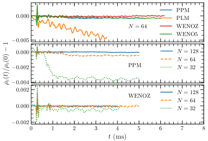
Figure 1: GRHD Evolution of central rest-mass density of the static star A0 model. Top: varying reconstruction at constant resolution $N=64$. Central: varying resolution for PPM reconstruction. Bottom: varying resolution for WENOZ reconstruction. Some data is cut to $5$ ms for visualization purposes.

Figure 1 shows the evolution of the central rest-mass density $\rho_{c}(t)$ for various reconstructions schemes and (for PPM and WENOZ reconstructions) for various resolutions. All the evolutions are stable over a period of several crossing times. The central rest-mass density shows the characteristic oscillations triggered by truncation errors. The latter are larger at the star surface, where a non-zero velocity field develops quickly. The oscillation frequencies extracted from the power spectra are compatible with the first three radial modes, namely $\nu_{F}=1462,3938$ and $5928$ Hz as computed in linear perturbation theory (Baiotti et al., 2009). The oscillations’ amplitude is below the percent level and converge to zero with increasing resolution. Low resolutions typically result in an unphysical expansion of the star beyond its initial radius. The use of the PLM reconstruction produces the largest expansion of the star, and it is effectively the least accurate scheme as noted also elsewhere, e.g. (Thierfelder et al., 2011a). The PPM scheme shows also a prominent drift in $\rho_{c}(t)$ at low resolutions ($N=32$) but for higher resolutions it retains a similar accuracy to the WENO schemes.

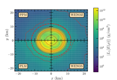
Figure 2: $L_{1}$ norm on the $x-y$ plane of the rest-mass density error of the static star model A0 for varying reconstruction. The dashed red line corresponds to the initial NS radius, contour levels corresponds to rest-mass densities of $\rho=[10^{4},10^{6},10^{8},10^{10},10^{12},10^{13},5\times 10^{13},10^{14},5\times 10^{14}]~{}{\rm g\,cm^{-3}}$. Data refer to GRHD evolutions at time $t=3.45$ ms and at at constant resolution $N=64$.

In Figure 2 we visualise the $L_{1}$ normed error of $\rho$,

$$L_{1}[E(\rho)](\mathbf{x},t):=|\rho(\mathbf{x},t)-\rho(\mathbf{x},0)|,$$ (29)

as a two-dimensional slice for the 4 different reconstruction schemes and $N=64$. This plot shows complementary information to the central density oscillation. The error of the PLM scheme is at all times worse than that in the other three schemes. The PPM scheme performs the worst at preserving the sharp star surface at early times (not shown in the plot), but at later times it has an overall lower error both at the surface and within the star itself away from the centre than the WENO schemes.

Figure 3: Convergence of $L_{1}[E(\rho)]$ norm of static star model A0 at $t=2.96$ ms. Data refer to GRHD evolutions and various reconstruction schemes. The modulus of the slopes, corresponding to the order of convergence is $1.85,1.76,1.87$ for PPM, WENOZ, WENO5 respectively.

The convergence of some of these results in the $L_{1}[E(\rho)]$ norm integrated on the whole computational domain are shown in Figure 3, with dashed lines showing linear extrapolations from the first two data points, the slopes of which indicate the order of convergence. All errors in the simulations converge at approximately second order rate. Consistent with the above discussion, the PPM scheme has the lowest absolute errors at the considered resolutions, with the convergent behaviour most consistent at all resolutions in the WENO simulations, especially WENOZ. At the lowest resolutions the WENO results stay within the convergent regime for the full duration of the simulation, whereas this does not happen for the lowest resolution PPM simulation, as seen in the lower two panels of Figure 1.

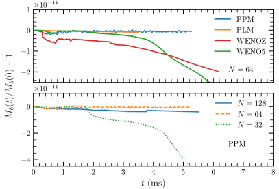
Figure 4: Baryon mass conservation along the GRHD evolution of static star model A0. The mass conservation can be violated due to the artificial low-density atmosphere as the fluid expands beyond the computational domain.

Figure 4 reports the relative violation of the baryon mass conservation within the simulation. The mass is conserved at the $10^{-11}$ relative level for all the schemes at the considered resolutions. The mass conservation is slightly violated due to the artificial low-density atmosphere and as the fluid expands beyond the computational domain. Hence, higher resolutions can reduce the violation by better resolving the surface and reducing the star’s expansion. In this respect, the PPM scheme performs best among those explored.

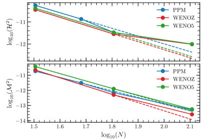
Figure 5: Top: Convergence of the $L_{1}$ norm of the Hamiltonian constraint of static star model A0. Bottom: Convergence of the $L_{1}$ norm of the momentum constraint of static star model A0. Data is evaluated at $t=2.96$ ms. The modulus of the slopes, corresponding to the order of convergence in the Hamiltonian (momentum) constraint is $3.51(4.41),3.65(5.46),3.64(4.88)$ for PPM, WENOZ, WENO5 respectively.

Finally, we inspect the convergence of the constraints in Einstein’s equations (see Eqs 18-20 in Daszuta et al. (2021)). The key property of the Z4c system is to propagate and damp the constraints during the evolution (Bernuzzi & Hilditch, 2010; Hilditch et al., 2013). For example, the norm of the Hamiltonian constraint is of order ${\sim}10^{-11}$ (${\sim}10^{-14}$) for the lowest $N=32$ (highest $N=128$) resolutions by end of the simulations. This value is typically several orders of magnitude smaller than the constraint violation in the initial data. For this reason, convergence properties might be difficult to interpret. Figure 5 shows the $L_{1}$-norm convergence of the Hamiltonian and momentum constraints by the end of the simulations. The observed convergence is approximately 4th or 5th order, depending on the reconstruction method, indicating that the finite differencing scheme used in the evaluation of the RHS of the Z4c equations is a significant source of error at this time.

4.2 GRHD evolution of Rotating Neutron Star

Next, we consider the evolution of a stable uniformly rotating equilibrium configuration close to the mass shedding limit. Specifically, we evolve the model AU4 of Dimmelmeier et al. (2006) that is rotating at a frequency of 655 Hz, with a corresponding rotational period of 1.53   ms. The initial data has baryon mass $M_{b}=1.506{\rm M_{\odot}}$ and gravitational mass $M=1.415{\rm M_{\odot}}$, and the same EOS as in Section 4.1. Initial data are generated using the RNS code of Stergioulas & Friedman (1995), which is incorporated into GR-Athena++ as an external shared library . The model is characterised by a central density of $\rho_{c}=5.453\times 10^{14}{\rm g\,cm^{-3}}$ and a polar-to-equatorial coordinate axis ratio of $r_{p}/r_{e}=0.698$. This is a challenging test where all the metric-matter source terms are non-zero and involving a sharp velocity profile at the star surface.

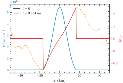
Figure 6: Profiles of velocity component $\tilde{u}^{y}$ and rest-mass density $\rho$ along the $x$ direction at the initial time and after two rotational periods. Data refer to resolution $N=32$ with PPM reconstruction. Note that velocity is plotted in geometric units.

Here we use the same grid set up as in Section 4.1 with the highest refinement level fully covering the star. The hydrodynamics evolution uses the PPM and WENOZ reconstructions. We do not consider magnetic fields in this test.

Figure 6 shows one-dimensional profiles of the rest-mass density and the velocity component $\tilde{u}^{y}$ for the lowest resolution $N=32$. For each quantity we show two profiles: the initial data (representing also the exact solution at each period) and the evolved data after the second rotational period. The density profile is well maintained within our evolution, and is visually indistinguishable from the initial profile. The velocity profile is well-simulated up to the lowest density regions, while the sharp spikes at the surface are not captured. Since no cutoff above the level of the atmosphere is used ($f_{\rm thr}=1$), fluid elements near the surface expand beyond the initial star radius. This is a common deficit of Cartesian finite-volume codes that can be improved with more sophisticated flux and reconstruction schemes (Kastaun, 2006; Guercilena et al., 2017; Doulis et al., 2022). Note that however, the overall angular momentum profile is largely unaffected by this inaccuracy.

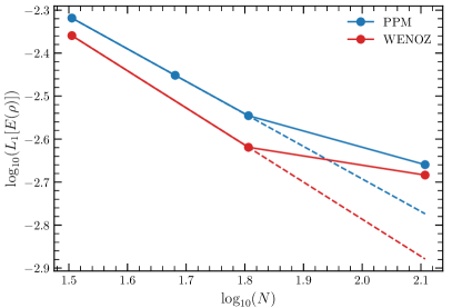
Figure 7: Convergence of $L_{1}$ norm of the error of the rest-mass density of rotating star AU4. Data refer to an evolution time of $t=3.06$ ms (second rotational period). The modulus of the slopes, corresponding to the order of convergence is $0.75,0.86$ for PPM, WENOZ, respectively.

Figure 7 shows the convergence of the $L_{1}$ norm of the difference between the rest-mass density profile and the initial density profile. The convergence rate is approximately first order, as expected since the surface dynamics dominate the error source. Mass conservation is in-line with the static star tests; relative variations are of order ${\sim}10^{-11}$ during the entire evolution for the lowest resolution.

4.3 Finite-temperature EOS evolution of Static Neutron Star

We now consider the SFHo EOS of Steiner et al. (2013) from the CompOSE database (Typel et al., 2015) to obtain a configuration similar to the A0 model described above. Taking a constant initial temperature of $T=0.1\ \mathrm{MeV}$ and assuming cold $\beta$-equilibrium ($\mu_{\mathrm{n}}=\mu_{\mathrm{p}}+\mu_{\mathrm{e}}$) gives us a 1-dimensional slice of the full table, which we use with a central density of $\rho_{c}=8.523\times 10^{14}\ {\rm g\,cm^{-3}}$ to solve the TOV equations. The result is a star with baryon mass $M_{b}=1.555\ {\rm M_{\odot}}$ and gravitational mass $M=1.4\ {\rm M_{\odot}}$. For the evolution we use the same grid setup as that described in Section 4.1, the PPM reconstruction method, and the PrimitiveSolver conservative-to-primitive library.

As with the baryon mass in Figure 4 we want to know to what degree the conservation of the scalar is violated. Analogously to Eq. (23), we define the “proton mass” $M_{p}$,

$$M_{p}=\int_{\Sigma_{t}}DY_{\mathrm{e}}{\rm d}^{3}x\,.$$ (30)

Note that this is conserved only because there are no reactions present in the simulation, and we use the name “proton mass” only as a parallel to $M_{b}$. As we expect this to be coupled strongly to violations in the conservation of baryon mass, we take the relative error of each quantity, $\mathrm{err}(Q,t)=(Q(t)/Q(0))-1$ for $Q=M_{b},M_{p}$, and then plot the ratio of these errors.

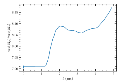
Figure 8: Ratio of the relative error in the baryon mass, $M_{b}$ (as defined in Eq. 23), to the “proton mass”, $M_{p}$ (Eq. 30), for $\sim 5\ \rm{ms}$ of evolution of a $M=1.4\ {\rm M_{\odot}}$ TOV star using the SFHo (Steiner et al., 2013) EOS.

Figure 8 shows the ratio of these errors for the aforementioned simulation setup. We see that the ratio of errors varies by $\sim 20\%$ through the course of the simulation, therefore the conservation of the scalar is maintained to approximately the same degree as the conservation of mass. If the relative error in the scalar came entirely from the error in the mass we would expect this error ratio to be $1$, whereas if there were some constant error of the same magnitude in $M_{b}$ and $M_{p}$ we would expect the ratio to be around $1/Y_{\mathrm{e}}$, which is $\sim 2$ in the atmosphere (most of the domain by volume), and $\sim 20$ in the core (where most of the mass lies) The rest-mass averaged value would be $\sim M_{b}/M_{p}\approx 17$. We see that the error falls within the range of expected values.

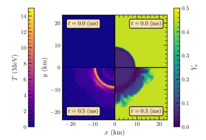
Figure 9: Temperature $T$ (left) and electron fraction $Y_{\mathrm{e}}$ (right) of the initial configuration (top) and after $0.5\ (\rm{ms})$ of evolution (bottom) of a $M=1.4\ {\rm M_{\odot}}$ TOV star using the SFHo (Steiner et al., 2013) EOS.

In Figure 9 we show the temperature, $T$, and electron fraction, $Y_{\mathrm{e}}$, of the fluid at the initial timestep, and after $\sim 10$ light crossing times of the star ($\sim 0.5\ \rm{ms}$). For the temperature we see the constant $T=0.1\ \rm{MeV}$ of the initial data at $t=0$, however after the evolution we see some heating on the surface of the star, causing it to reach $T\approx 15\ \rm{MeV}$. This effect (seen in many other simulations, e.g. (Perego et al., 2019; Endrizzi et al., 2020; Prakash et al., 2021)) is driven by artificial shock heating as the sound speed falls off towards the edge of the star (Gundlach & Leveque, 2011). Additionally, we see a smaller increase in temperature in the core of the star, reaching around $T\approx 5\ \rm{MeV}$ in places. This effect comes from the poor condition number of the temperature with respect to the conserved energy $\tau$ (Hammond et al., 2021): small errors in $\tau$ due to, for example, interpolation of the spherically symmetric initial data onto the cartesian grid used in the evolution can be amplified by many orders of magnitude into errors in $T$ at high densities and low temperatures as the total energy of the fluid is very weakly dependent on $T$ under these conditions. For the electron fraction, we see at $t=0$ the expected equilibrium configuration of the electron fraction: a low $Y_{\mathrm{e}}\approx 0.05-0.1$ core surrounded by a higher $Y_{\mathrm{e}}\approx 0.45-0.5$ atmosphere. After the evolution we see that some of the low $Y_{\mathrm{e}}$ matter has begun to boil off the surface of the star, which, as mentioned in Section 4.2, is a common artefact seen in simulations of this kind. The increase we see in Figure 8 is likely due to this effect.

4.4 Long-term Magnetic field dynamics in Static Neutron Star

The dynamics and re-configuration of an initially poloidal magnetic field in a static NS remains an open problem in neutron star physics. A poloidal magnetic field configuration is unstable on Alfven timescales e.g.  (Tayler, 1957, 1973; Wright, 1973; Markey & Tayler, 1973, 1974; Flowers & Ruderman, 1977; Braithwaite & Spruit, 2006) and understanding magnetic field topology and energy re-distribution requires long-term numerical relativity evolutions, e.g. (Kiuchi et al., 2008; Lasky et al., 2011; Ciolfi et al., 2011; Pili et al., 2017; Sur et al., 2022).

Here, we consider GRMHD evolutions of model A0 with a superposed poloidal magnetic field given by the vector potential (Liu et al., 2008)

$$(A_{x},A_{y},A_{z})=(-yA_{\varphi},xA_{\varphi},0)$$ (31a)

$$A_{\varphi}:=A_{b}\max(p-0.04\,p_{\rm max},0)$$ (31b)

where $p_{\mathrm{max}}$ is the maximum value of the pressure within the star. The parameter $A_{b}$ controls the magnitude of the magnetic field, and is set to obtain a maximum value of $1.84\times 10^{16}$ G inside the star. We use the WENOZ scheme and the same grid setup as for the model A0 in Section 4.1. We observe similar features for the performance of the code in the case of GRMHD as in the above GRHD simulations. We do not repeat here the discussion and instead, discuss GRMHD effects following Sur et al. (2022). In contrast to the simulations presented in Sur et al. (2022) which were performed in the Cowling approximation, we now evolve the full dynamical spacetime. Due to the lack of implemented constraint preserving boundary conditions for the Z4c equations, we must adopt a different grid configuration to our previous simulations, with outer boundaries pushed further away. Consequently we use the same grid set up as in Section 4, with resolutions $N=32,64,128$ closely matching the resolution over the NS itself in simulations pS64, pS128, pS256 respectively in Sur et al. (2022).

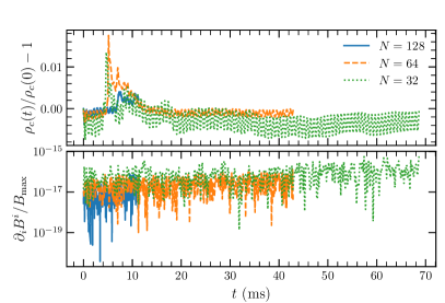
Figure 10: Top: Evolution of central rest-mass density of the static star A0 model with superposed poloidal magnetic field with WENOZ reconstruction. Bottom: Integrated divergence of magnetic field (Eq. (18)) normalised by maximum value of the magnetic field.

In the upper panel of Figure 10 we see the oscillations of the central density of the star. Excited by the superposed magnetic field these are larger in magnitude than those in Figure 1, with a peak in the oscillations corresponding to the saturation of the growth of $b^{\phi}$ as seen below.

The constrained transport algorithm is designed to preserve the divergence-free condition on the magnetic field on the face centred grid. As a first check, we show this is indeed the case for our simulations. The lower panel of Figure 10 shows the integrated value of the divergence-free constraint over time at different resolutions as normalised by the maximum value of $|B|$. The total relative violations oscillate at the level of ${{\sim}10^{-16}}$ at the lowest resolution.

We observe the onset of the well known “varicose” and “kink” instabilities by visualising the evolution of magnetic field streamlines in the equatorial plane. In Figure 11 we track the evolution of streamlines seeded on a circle in the equatorial plane of radius $5.91$ km. After $4.93$ ms (left panel) we see the rotational invariance of the magnetic streamlines is broken, with the onset of the varicose instability altering the cross sectional area of these streamlines. As the evolution progresses further we see some signs that the streamlines are further disrupted orthogonal to the equatorial plane in the onset of the kink instability, which we identify with the saturation of the growth in $b^{\phi}$ (see below), as can be seen by $12.8$ ms (middle panel). We finally show the late time appearance of the field after its non-linear rearrangement, at $44.3$ ms (right panel). Here while we see an overall poloidal structure, the field configuration has grown clear toroidal components.

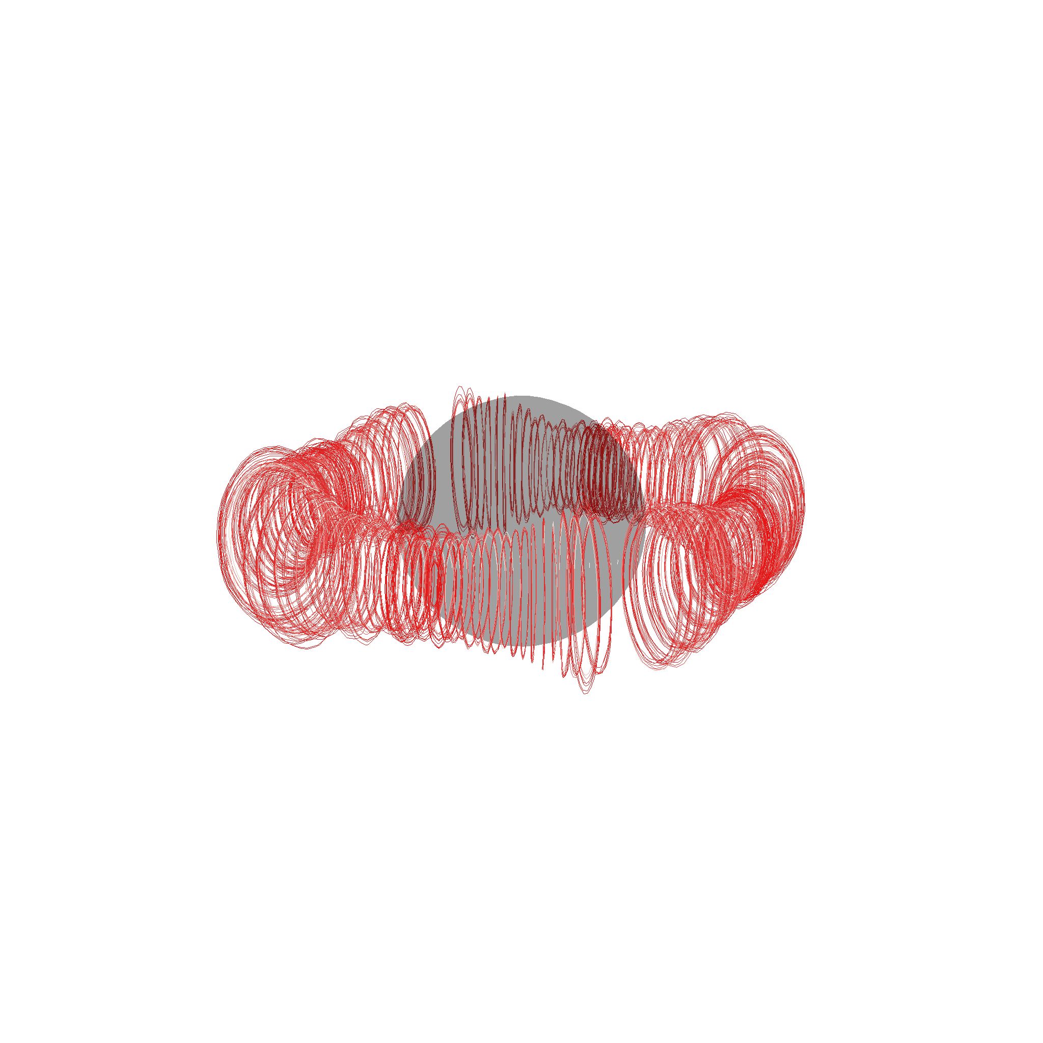
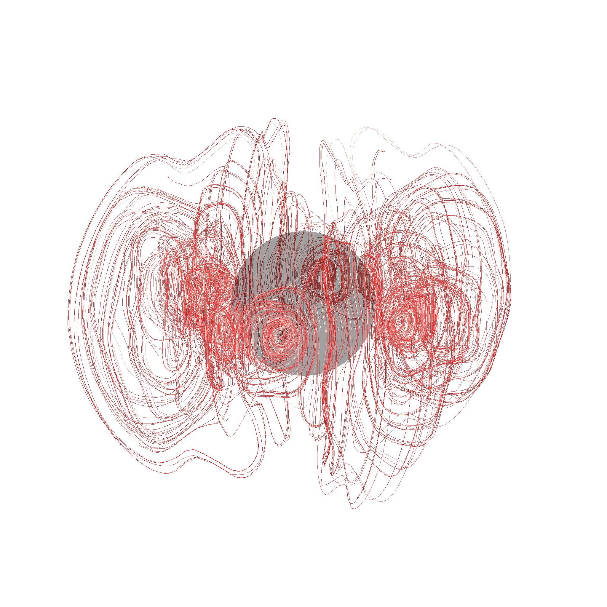
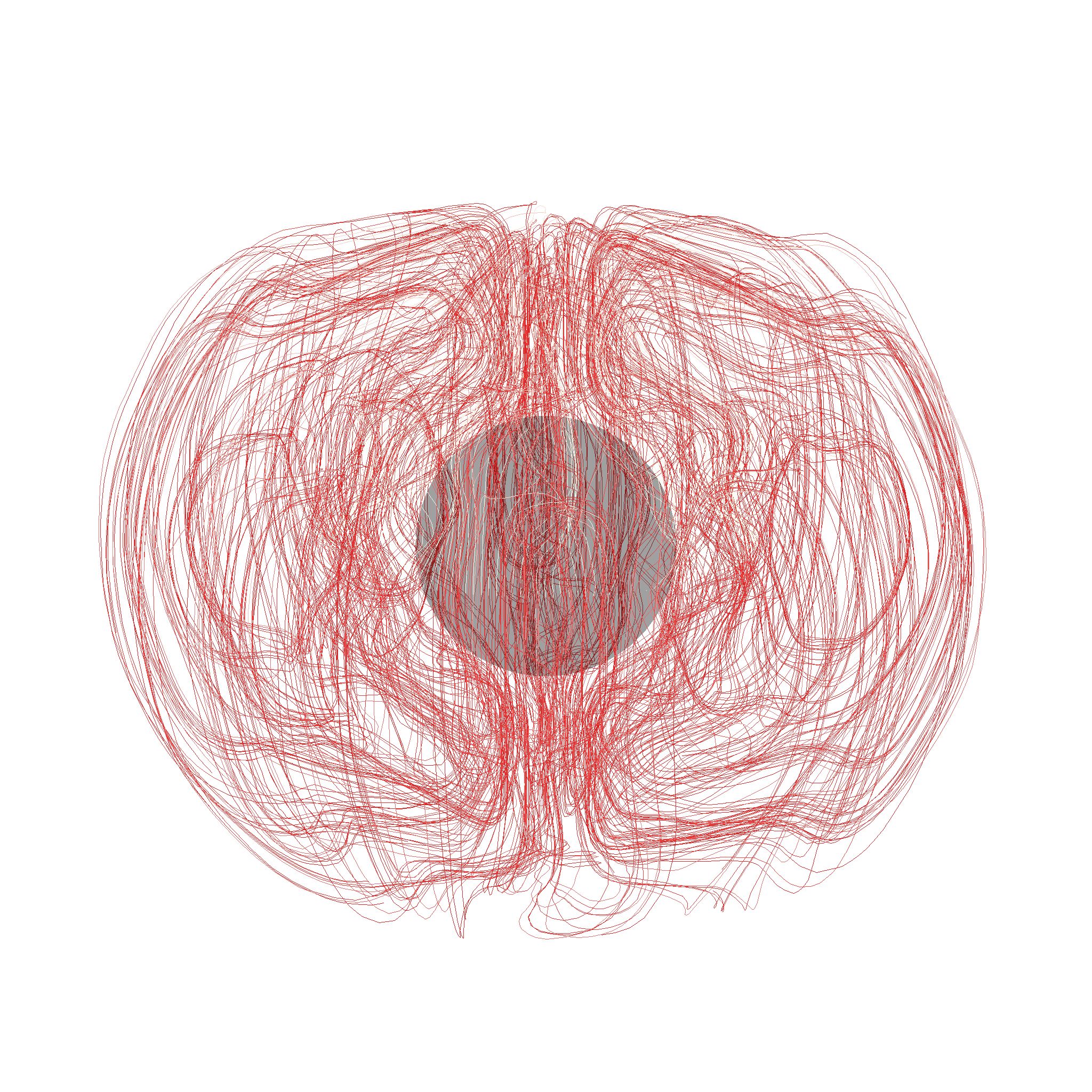
Figure 11: Evolution of magnetic streamlines seeded in equatorial plane at radius $5.91$ km. Gray isocontour shows surface of $\rho=6.18\times 10^{14}{\rm g\,cm^{-3}}$. Left: Varicose instability at $t=4.93$ ms. Middle: Kink instability at $t=12.8$ ms. Right: Late time non-linear field arrangement $t=44.3$ ms.

The initially poloidal magnetic field is unstable, and so we observe the growth of the toroidal component of the magnetic field, measured by $b^{\phi}b_{\phi}$. In the upper panel of Figure 12 we see that, after $\sim{}16$ ms, the toroidal component grows to form $\sim{}10\%$ of the total magnetic field energy, with the onset of the growth of this component delayed as a function of resolution. This behaviour matches previously observed behaviour in the Cowling approximation, demonstrated in Figure 3 of Sur et al. (2022).

In the lower panel of Figure 12 we track the relative changes in the energies arising from kinetic energy $E_{\mathrm{Kin}}$, magnetic energy $E_{B}$, internal energy $E_{\mathrm{int}}$ and the rest mass $D$. We see that as the magnetic field instabilities drive the rearrangement of the field, the kinetic energy of the fluid correspondingly increases, with local maxima in the kinetic energy corresponding to local maxima in the growing toroidal field, corresponding also to a loss in overall magnetic energy. We note also that the internal energy is well preserved in this simulation, in contrast to the enthalpy which was seen to grow in Figure 5 of Sur et al. (2022). We attribute this to an improved atmosphere treatment, and the increased grid size in comparison to the previous simulations.

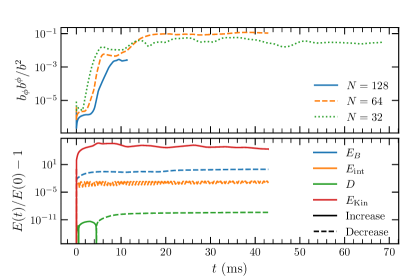
Figure 12: Top: Growth of the toroidal component of magnetic field energy as a fraction of total magnetic field energy. Bottom: relative change in magnetic energy, internal energy, mass and kinetic energy for $N=64$. Solid lines denote a positive change in energy, dashed lines denote a negative change.

5 Gravitational collapse of Rotating Neutron Star

In this section we benchmark GR-Athena++ against the gravitational collapse of a rotating NS to a BH. Initial data are the unstable, uniformly rotating D4 equilibrium configuration previously studied in several works, e.g. (Baiotti et al., 2005; Reisswig et al., 2013; Dietrich & Bernuzzi, 2015). The D4 model is spinning close to the mass-shedding limit at a frequency of $1276$ Hz and it has baryon mass and gravitational mass of, respectively, $M_{b}=2.0443{\rm M_{\odot}}$ $M=1.8604{\rm M_{\odot}}$. The initial data are calculated using the RNS code and imposing a central density of $\rho_{c}=1.924388\times 10^{15}{\rm g\,cm^{-3}}$ and a polar-to-equatorial coordinate axis ratio of $r_{p}/r_{e}=0.65$. Collapse is triggered by adding a $0.5\%$ perturbation to the fluid pressure as in Dietrich & Bernuzzi (2015).

We perform simulations at multiple grid resolutions for the PPM reconstruction method. The grid is composed of eight static refinement levels with $N=32,64,128$ and reaching a maximum resolution of $92.2,46.1,23.1$ m respectively. The outer boundaries of the grid are the same as in Section 4.1, while the innermost 3 refinement levels are located within the initial radius of the star. In contrast to previous work we do not employ any grid symmetry. Both reconstructions successfully handle BH formation and the subsequent evolution of the latter without the use of excision.

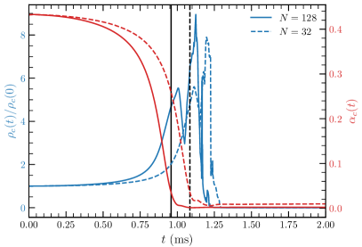
Figure 13: Evolution of central rest-mass density and lapse of collapsing D4 model. Data from PPM simulations are shown at different resolutions. Vertical black lines denote collapse time for each simulation. We note that the oscillatory behaviour occurs within the horizon, after collapse.

Figure 13 shows the central density and lapse during the collapse. As the density increases toward the central region, the curvature increases and the lapse collapses as a result of the gauge conditions. Black hole formation is handled by the moving puncture gauge conditions adopted for the simulations (Thierfelder et al., 2011b). For this simulation we employ no excision of the hydrodynamical variables within the horizon, in contrast to e.g. (Bernuzzi et al., 2020), with mass loss from the grid occurring as the determinant of the spatial metric blows up at the origin. An apparent horizon  (AH) is found at about one millisecond from the start of the simulation. Until this point, the run shows excellent mass conservation with a relative error of $10^{-13}$ up to collapse. We note that, since the initial grid configuration contains refinement levels within the star, this provides a robust test of the mass conservation provided by the flux correction operators described in (Stone et al., 2020). Afterwards, baryon mass is lost as shown in Figure 14. The AH returns a Christodoulou mass (Christodoulou, 1970) of $M_{\rm BH}=1.857{\rm M_{\odot}}$ and an angular momentum $J_{\rm BH}=1.884{\rm M_{\odot}}^{2}$G/c. These values are affected by relative uncertainties of order $10^{-3}$ for the lowest resolution simulation $N=32$, which improves as a function of resolution. These results favourably compare to the results presented in (Reisswig et al., 2013; Dietrich & Bernuzzi, 2015).

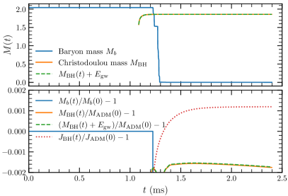
Figure 14: Top: Evolution of baryon mass and black hole (Christodoulou) mass in collapsing D4 model for $N=32$. The dashed line shows the sum of the black hole mass and the gravitational-wave energy in the $(2,0)$ mode extracted at the coordinate sphere. Bottom: Baryon mass and angular momentum conservation and relative differences of Christodoulou mass and with respect to the initial ADM mass.

Finally, we calculate the gravitational waveforms associated to the collapse. Figure 15 shows the $(\ell,m)=(2,0)$ multipole of the strain reconstructed from the Weyl scalar (Daszuta et al., 2021) using a time integration and corrected by a polynomial drift (Baiotti et al., 2009). Waveforms are extracted at coordinate spheres centered at the origin of the Cartesian grid, constructed by sampling geodesic spheres, and of radius $R=221$ km. They are shown as a function of the retarded time to the extraction spheres, given by $t-r_{*}$ with $r_{*}=r+2M\log(r/2M-1)$, and $r(R)$ the areal radius of the spheres of coordinate radius $R$ (the isotropic Schwarzschild radius).

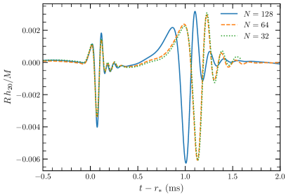
Figure 15: Gravitational waveforms of collapsing D4 model. Data from PPM simulations are shown at all resolutions for the dominant $(\ell,m)=(2,0)$ multipole of the strain. The waveform is shown as a function of the retarded time to the extraction sphere. At $N=32$ the resolution is too low to observe convergent behaviour, though at higher resolutions we do see convergence in the waveforms at approximate first order. Note the y-axis is plotted in geometric units.

After an initial burst of physically spurious so-called “junk” radiation, the waveform has the well-known “precursor-burst-ringdown” morphology expected for the collapse. The amplitude’s relative maximum at around $t-r_{*}\simeq 1$ ms corresponds to AH formation, while the amplitude’s absolute maximum is produced after BH formation. The black hole’s quasi normal ringing follows the waveform peak and is consistent with a perturbed Kerr metric (Dietrich & Bernuzzi, 2015). Overall, these tests indicate GR-Athena++ can handle gravitational collapse and delivers reliable results at relatively low resolutions and without grid symmetries.

6 Binary Neutron Star spacetimes

This section presents tests that involve BNS spacetimes. We discuss simulations of a quasi-circular, equal-mass merger with and without magnetic fields. Irrotational constraint-satisfying initial data are generated for a binary of baryon mass $M_{b}=3.2500{\rm M_{\odot}}$ and gravitational mass $M=3.0297{\rm M_{\odot}}$ at an initial separation of $45$ km. The Arnowitt-Deser-Misner (ADM) mass of the binary is $M_{\rm ADM}=2.9984{\rm M_{\odot}}$, the angular momentum $J_{\rm ADM}=8.83542{\rm M_{\odot}}^{2}$G/c, and the initial orbital frequency is $f_{0}\simeq 294$ Hz. These data are computed with the Lorene library (Gourgoulhon et al., 2001) and are publicly available . Here we use the ideal gas EOS with $K=124$. For magnetised binaries, the magnetic field in each star is initialised as in the single star case with the vector potential in Eq. (31b), with $A_{b}$ chosen to give a maximum value of $1.77\times 10^{15}G$. We first benchmark GRHD evolutions and GWs against similar results obtained with the BAM code (Brügmann, 1996; Brügmann et al., 2008; Thierfelder et al., 2011a). We then focus on GRMHD evolutions and showcase the use of GR-Athena++’s AMR for investigating the Kelvin-Helmholtz instability developing at the merger’s collisional interface.

For all purely hydrodynamical runs described in this section, the grid outer boundaries are set at $[\pm 2268,\pm 2268,(0,2268)]$ km, with bitant symmetry enforced in the $z$ direction. For GRMHD simulations, no symmetry is enforced, and the outer boundaries are set at $[\pm 2268,\pm 2268,\pm 2268]$ km. Initially a refined static grid is defined consisting of 7 levels of refinement, with the innermost grid covering both stars, extending from $[\pm 37,\pm 37,\pm 37]$ km, or $(0,37)$ km in the $z$ direction if bitant symmetry is enforced across the $z=0$ plane. We perform runs at three base level resolutions, $N=64,96,128$, corresponding to a grid spacing on the finest refinement level of $(554,369,277)$ m respectively. Simulations are performed with the WENOZ reconstruction, and hydrodynamical variables are excised within the apparent horizon for runs with GRMHD.

6.1 Benchmark against BAM

The binary revolves for about three orbits before forming a massive remnant that undergoes gravitational collapse after about ${\sim}19$ ms from the beginning of the simulation for the lowest resolution simulation with GRHD. We demonstrate 3 snapshots of the evolution of a magnetised binary in Figure 16; at $t=5.96$ ms, shortly before merger; $t=7.83$ ms, approximately the moment of merger; and $t=16$ ms, shortly before gravitational collapse to a BH, at which point an apparent horizon is found. We overlay the structure of the Mesh, with each black square representing a single MeshBlock of $16^{3}$ cells. The baryon mass conservation is shown in Figure 17 for both the GRHD and GRMHD evolutions and for different resolutions. We find somewhat larger violations of mass conservation with respect to the single star test, however, the maximum relative variation remains at ${\sim}10^{-6}$ level at the lowest resolution. This value is more than sufficient to robustly study mass ejecta and comparable to other state-of-the-art Eulerian codes at the considered resolutions, e.g. (Radice et al., 2018). Our experiments with the atmosphere parameters highlighted that simulations with the best mass conservation are obtained by setups that lead to a mass increase (rather than decrease).

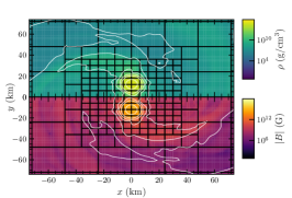
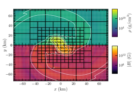
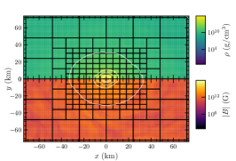
Figure 16: Snapshots of rest-mass density (upper half) and magnetic field strength (lower half) in the orbital plane. The snapshots correspond to the final orbit ($t=5.96$ms), the moment of merger ($t=7.83$ms), conventionally defined as the moment at which the $(\ell,m)=(2,2)$ mode of the gravitational wave has the amplitude peak, and a late stage shortly before gravitational collapse $t=16$ms. White contours are lines of constant density at values $\rho=(6.18\times 10^{14},3.09\times 10^{14},6.18\times 10^{13},6.18\times 10^{12},6.18\times 10^{10},6.18\times 10^{8},6.18\times 10^{6},6.18\times 10^{4}){\rm g\,cm^{-3}}$

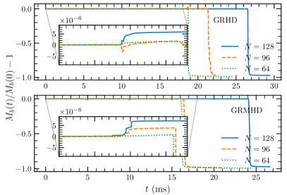
Figure 17: Baryon mass conservation along the GRHD and GRMHD evolutions of the binary neutron star model. To the moment of merger, $t\simeq 7.5$ ms, the maximum relative violation is of the order $10^{-7}$. After merger, the violation increases to the $10^{-6}$ level. Note the mass typically increases rather than decreasing due to the accretion of the atmosphere. The sudden drop of the mass at late times is due to black hole formation.

The GR-Athena++ evolutions are in qualitative agreement with previous BAM simulations (Thierfelder et al., 2011a). For a quantitative benchmark, we perform here two new BAM simulations using six refinement levels, two of which are moving following the stars. The finest refinement level covers entirely the star at a resolution of ${\sim}461$ m, that is comparable with GR-Athena++ $N=64$. One BAM simulation uses a finite volume method similar to GR-Athena++ and based on the WENOZ reconstruction (Bernuzzi et al., 2012). The other uses the entropy flux-limited (EFL) scheme of Doulis et al. (2022), which is a fifth-order accurate finite-differencing scheme also making use of the WENOZ reconstruction. This run is conducted with the best hydrodynamics scheme available to date for these binary simulations.

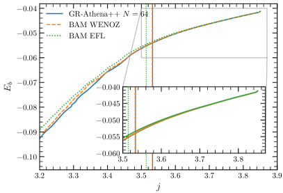
Figure 18: Binding energy vs angular momentum curves $E_{b}(j)$ for GR-Athena++ and BAM simulations. These quantities are computed following Damour et al. (2012); Bernuzzi et al. (2012); they are rescaled by the mass, and shown in geometric units. The moment of merger of each dataset is shown as vertical line. The inset zooms-in on the energetics during the orbital phase, prior to the moment of merger. Note the initial adjustment related to the use of conformally flat initial data and “junk” radiation.

A gauge-invariant description of the dynamics of binary spacetimes is given by curves of binding energy and angular momentum (Damour et al., 2012; Bernuzzi et al., 2012), which we use to compare evolutions. In line with the above references we define the binding energy $E_{b}=(M_{\mathrm{ADM}}-E_{\mathrm{GW}})\nu/(M-1)$ and the angular momentum $j=(J_{\mathrm{ADM}}-J_{\mathrm{GW}})/(M^{2}\nu)$, with $\nu$ the symmetric mass ratio, $\nu=q/(1+q)^{2}$, $q>1$ the mass ratio and quantities suffixed with $\mathrm{GW}$ the contributions radiated away in gravitational waves.

The energy curves for our simulations are shown in Figure 18; note these quantities are commonly shown in geometric units. The evolution proceeds from right to left, as the binary loses angular momentum and becomes more bound. The agreement between GR-Athena++ and BAM is excellent, already at these low resolutions. Differences between the simulations are more evident towards the moment of merger (vertical lines) and afterwards. As is clear from the comparison of the two BAM simulations, these differences are mainly due to the hydrodynamics scheme and are in particular affected by the choice of the reconstruction scheme. We note that a key difference between BAM and GR-Athena++’s implementation of the hydrodynamics schemes comes in the choice of the reconstructed primitive variables. GR-Athena++ reconstructs the fluid pressure $p$, while BAM reconstructs the specific internal energy $\epsilon$. Experimentation with this reconstruction choice in GR-Athena++ leads to noticeable variations in the evolution as expected, though we find more robust performance in GR-Athena++ when reconstructing the pressure. GR-Athena++ also requires the intergrid interpolations discussed in Section 3.2 absent in BAM, which uses a cell centred grid for evolving the Einstein equations. Finally the grid structures between these two codes are different, with BAM utilising a nested box-in-box style refinement approach, as opposed to the block-based oct-tree structure of GR-Athena++.

Finally, we compare the gravitational waveforms by discussing in Figure 19 the dominant $(\ell,m)=(2,2)$ mode of the radiation. The different simulations mostly differ in the waveform phase. At the lowest considered resolution the GR-Athena++ simulation merges slightly earlier than the BAM WENOZ and EFL. This possibly indicates that the overall GR-Athena++ scheme and grid choice leads to more numerical dissipation than the BAM runs (Bernuzzi et al., 2012; Radice et al., 2014b), however, the time of collapse of all three runs happens within a time interval of ${\sim}2.5$ ms, indicating a substantial agreement of the computations. The gravitational frequencies at the moment of merger (middle panel) are very close to each other, $\omega_{22}\simeq 1340$ Hz for GR-Athena++ and BAM WENOZ and $\omega_{22}\simeq 1360$ Hz for BAM EFL; as are the remnants’ frequency evolution. After collapse, the quasi normal mode frequencies of the remnant black hole are poorly resolved for all three runs at the considered resolution, but are compatible with the fundamental mode frequency $\nu_{\rm QNM}\sim 6.5$ kHz ($M\omega_{22}\simeq 0.57$ in geometric units).

The bottom panel of Figure 19 quantifies the phase differences of the GR-Athena++ $N=64$ run with respect to the BAM runs and the GR-Athena++ runs at higher resolutions. The difference between the $N=64$ and $N=128$ runs is rescaled according to Eq. (26) to compare to the difference between the $N=64$ and $N=96$ run assuming second order convergence. These curves closely match up to merger suggesting second order convergence during the inspiral phase. Further, the difference to the BAM runs significantly reduces at higher resolutions.

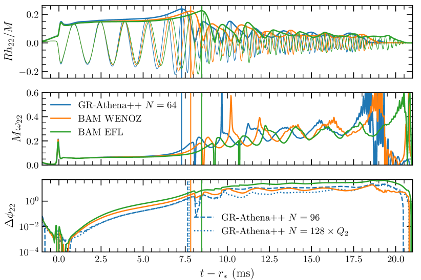
Figure 19: Waveform analysis and comparison with BAM. Top: Real part and amplitude of the $(\ell,m)=(2,2)$ mode of the strain. We show GR-Athena++ data with WENOZ reconstruction and $N=64$ and BAM data with finite volume scheme and WENOZ reconstruction and with the EFL scheme at a similar resolution. The y-axis is plotted in geometric units. Middle: Instantaneous frequency of the waves for the three datasets. The y-axis is plotted in geometric units. Bottom: phase differences between the GR-Athena++ data $N=64$ and GR-Athena++ data at higher resolution $N=96$ (dashed) and $N=128$ (dotted lines), and BAM data. GR-Athena++ phase difference data at $N=128$ is rescaled assuming second order convergence, matching with the $N=96$ data up to merger. The moment of merger of each dataset is shown as vertical line.

6.2 Kelvin-Helmholtz instability

During the merger of a BNS the magnetic field in the initial NSs can be amplified through a variety of instabilities triggered throughout the merger process. These amplifications can lead to the large magnetic fields present in the remnant star which may be required to launch relativistic jets that can be the source of the observed gamma ray bursts from the BNS merger associated to GW170817. One such instability is the Kelvin-Helmholtz instability (KHI), triggered when a shearing interface between the two stars is created, at the moment of first contact between the stars. This creates small scale vortex like structures in the fluid, associated to an amplification in the magnetic field (Price & Rosswog, 2006). Such amplifications have been extensively studied through numerical simulations (Kiuchi et al., 2015, 2018; Palenzuela et al., 2022; Aguilera-Miret et al., 2023). Here we aim to use the flexible AMR of GR-Athena++ to efficiently resolve the KHI, with a targeted refinement criterion. Here we present the results of four simulations, two with static grids set up as described in Section 6, with resolution $N=64,128$, referred to here as SMR64 and SMR128, and two AMR runs initialised from the SMR64 run at $t=4.93$ms, but allowed to refine by one further level, thus matching the resolution of the SMR128 run on the finest grid level. The magnetic fields are initialised as in Section 6. The first criterion for refinement is given by the maximum value of $|B|$ on the MeshBlock, with a block refined if $|B_{\mathrm{max}}|$ exceeds $8.35\times 10^{13}$G and derefined if lower than this value. We refer to this run as AMRB. The second criterion is determined by the quantity

$$\sigma=\sqrt{((\Delta_{x}\tilde{u}^{y})^{2}+(\Delta_{y}\tilde{u}^{x})^{2})},$$ (32)

with $\Delta_{i}$ the undivided difference operator in the $i$th coordinate direction, which monitors the shear of the fluid velocity. MeshBlocks are refined if $\sigma>4.50\times 10^{9}cm/s$ anywhere within the block, and if the maximum density within the block exceeds a threshold value, in order to avoid overrefining unphysical low-density regions, and they are derefined if $\sigma<2.25\times 10^{9}cm/s$. We refer to this run as AMR$\sigma$. In both cases, derefinement is only permitted as long as the resolution does not drop below that of SMR64. Threshold values of $|B_{\mathrm{max}}|$ and $\sigma$ employed are determined by numerical experimentation.

We demonstrate the appearance of the grid evolution in Figure 20, a snapshot at approximately the moment of merger at $t=7.88$ms of run AMR$\sigma$. Here the grid structure and density isocontours are shown for values of $\rho>10^{11}{\rm g\,cm^{-3}}$, with the $z>0,~{}y<0$ quadrant cut away for visualisation purposes. We see that, at the interface between the stars, higher resolution MeshBlocks have been generated in the region where the KHI driven amplification can be expected to occur.

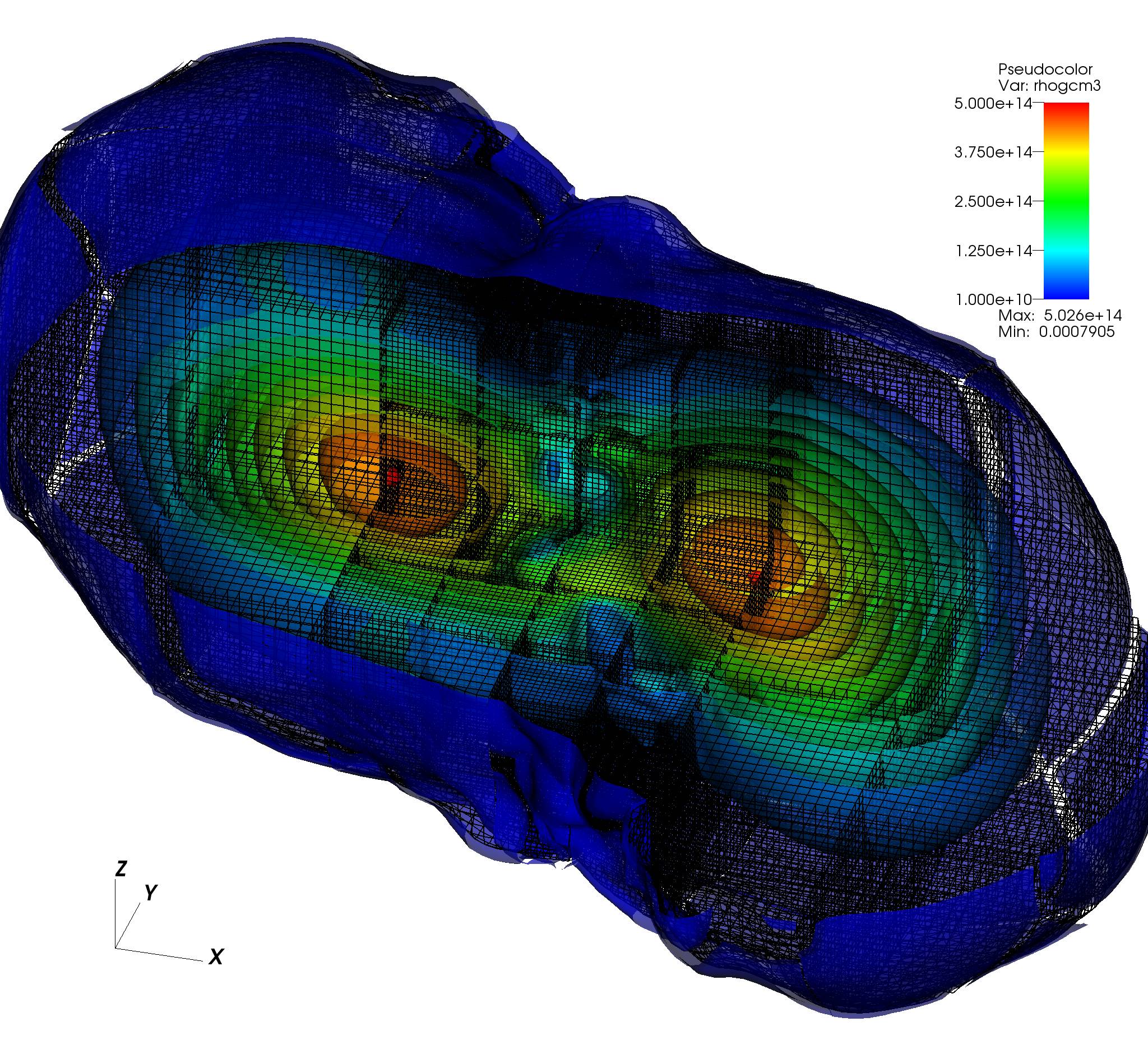
Figure 20: Snapshot of Mesh structure at $t=7.88$ms shortly before merger in run AMR$\sigma$. Isocontours of density are also shown for $\rho>10^{11}{\rm g\,cm^{-3}}$. For visualisation purposes the $z>0,~{}y<0$ quadrant has been cut out.

To measure the effectiveness of the AMR criteria we demonstrate the amplification of the magnetic field $|B^{2}|$, as a measure of the magnetic energy, for the four runs described above, as well as the growth of the number of MeshBlocks in the AMR runs, which serves as a measure of computational cost. We note that, due to the global timestep of Athena++, as soon as the AMR runs create a block on the highest refinement level, the global timestep drops to match that of the run SMR128.

In the upper panel of Figure 21 we see the amplification of the magnetic field energy. For SMR128 we see that the energy is amplified by a factor of over 25 after the moment of merger, at $t\sim 10.2~{}$ms, through the KHI. The AMR simulations manage to capture some of this amplification, with AMRB capturing an amplification of a factor of 7.85, while AMR$\sigma$ only captures a factor of 3.26. We note that Kiuchi et al. (2015), at considerably higher resolutions of $17.5$m see a much larger amplification, of 6 orders of magnitude, from a much weaker initial magnetic field profile, of initial strength order $10^{13}$G. We expect that the addition of further levels of mesh refinement may be able to capture such larger amplifications, as well as the possibility of improved performance through fine-tuning of the threshold values used in the AMR criteria.

We also demonstrate the number of MeshBlocks generated in each simulation, as a measure for the computational cost, in the middle panel of Figure 21. We see that the run AMRB generates considerably fewer MeshBlocks than the run SMR128 during the amplification of the field, with a factor of 1.79 fewer MeshBlocks at the time of the peak in magnetic energy, and a factor 1.91 fewer at the moment of merger itself. This suggests that targeted use of AMR in GR-Athena++ can allow us to resolve small features without drastically increasing the computational cost, in contrast to a SMR grid configuration. In contrast we see that the criterion based on $\sigma$ captures less of the magnetic field amplification, and generates more MeshBlocks than the SMR128 run. This criterion seems less suited to purely capturing the magnetic field amplification, but generates extra MeshBlocks in lower density regions, at the star surface, and in the vicinity of matter disrupted from the binary system. In this simulation however, we see superior conservation of mass, compared to both the SMR and other AMR runs, and note that such an AMR criterion may prove useful in tracking ejected matter for simulations with microphysical EOSs.

In the lower panel of Figure 21 we see the violation of the divergence-free condition on the magnetic field, Eq. (18), integrated over the computational domain, as normalised by the maximum value of $|B|$, similar to the lower panel of Figure 10. Through the AMR runs we see at worst a total relative error of $10^{-14}$ in this constraint. This value is larger by an order of magnitude than those for the SMR runs, but is maintained at a low level even though MeshBlocks are continually created and destroyed as can be seen in the middle panel, verifying that the divergence and curl preserving restriction and prolongation operators implemented in (Stone et al., 2020) of (Tóth & Roe, 2002), are sufficient for the accurate performance of long-term BNS evolutions with magnetic fields and AMR.

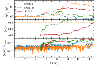
Figure 21: Top: Amplification of total magnetic field strength $|B^{2}|$ in BNS merger for SMR with resolution $N=64,128$ and AMR criteria based on the maximum $B$ field (AMRB) and velocity shear $\sigma$, (AMR$\sigma$). Middle: Total number of MeshBlocks present in each run. Bottom: $\partial_{i}B^{i}$ integrated over the computational domain, normalised by the maximum value of the magnetic field.

7 Scaling tests

In order to demonstrate the performance of GR-Athena++ on large problems we perform scaling tests on several target machines, namely SuperMUC-NG (hereafter SuperMUC), HLRS-HAWK (hereafter HAWK) and Frontera, running with both OpenMP and MPI parallelizations. We consider SMR grid setups and different problems, namely a single TOV star and a binary system consisting of two boosted TOV stars; both problems are run with and without magnetic fields. When magnetic fields are included, the configuration matches that in Eq. (31b). Scaling performance is important for both problems; for the binary problem we want to be able to efficiently run at high resolution during the inspiral for the extraction of highly accurate gravitational waveforms, while, at late times, high resolution simulations of GRMHD processes in the post merger remnant require quality scaling on a grid setup tuned to a single star. In all the scaling tests presented $N_{B}=16$, and we evolve 20 timesteps.

7.1 Strong scaling tests

The strong scaling tests are conducted as follows. We construct a cubic SMR grid with the same physical extent as in Section 6 with the same initial configuration of NSs. We perform several strong scaling series by selecting different resolutions, allowing us to explore the scaling properties at different numbers of cores. Each series is then labelled by $N$, which corresponds to a given resolution. For each resolution the extent of the most refined region is tuned in order to achieve similar MeshBlock/core ratios across all resolutions. We present results obtained by utilising all the available cores in a node, namely using 48 cores (12 MPI tasks per node and 4 OpenMP threads per task) for SuperMUC and 128 cores (32 MPI tasks per node and 4 OpenMP threads per task) for HAWK. We discuss the scaling properties, calculating the scaling efficiency as

$$\mathrm{~{}Efficiency~{}~{}}=1-\frac{t-t_{\mathrm{ideal}}}{t_{\mathrm{ideal}}},$$ (33)

where $t$ is the elapsed wallclock time and $t_{\mathrm{ideal}}$ is the time expected if the code had perfect strong scaling, halving exactly when resources were doubled.

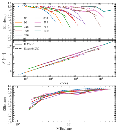
Figure 22: Scaling efficiency (see Eq. (33)) for the binary neutron star configuration with MHD. Results for both HAWK and SuperMUC are included, up to $\mathcal{O}(10^{5})$ cores. Top: efficiency versus number of cores. Middle: zone cycles per second ($Z$) versus number of cores. Bottom: efficiency in terms of the MeshBlocks/core ratio.

In Figure 22 we show the scaling efficiency calculated from our strong scaling tests for the magnetised binary, performed on both SuperMUC and HAWK clusters. In the top panel we demonstrate very good strong scaling efficiencies for all resolutions, i.e.in all regimes of number of cores. In particular, we find efficiencies in excess of $80\%$ up to $\sim 10^{5}$ cores (gray and teal lines) for both SuperMUC (dashed lines) and HAWK (solid lines). In the scaling tests on HAWK, for some resolutions (e.g.pink and brown lines), we observe a faster initial drop in efficiency compared to the tests on SuperMUC. After this drop, however, the efficiency settles at a constant value $\sim 85\%$ and decreases again to $\sim 70\%$ only when the load goes below 4 MeshBlocks/core (see third panel). The bottom panel of Figure 22 shows that the efficiency on SuperMUC is $\gtrsim 90\%$ as long as $\mathrm{\texttt{MeshBlock}s/core}\gtrsim 6$. We attribute such different behaviours to the different architectures of the two computer clusters. This causes a difference in the raw performance in terms of zone cycles per second ($Z$) (middle panel), where we note that runs on HAWK are a factor $\gtrsim 2$ faster than the runs on SuperMUC.

We note that we find comparable results also for the binary problem without magnetic field evolution, and the single star evolution with and without magnetic fields.

7.2 Weak scaling tests

We measure the performance of weak scaling by measuring the zone cycles per second $Z$ performed by the code, with the expectation that for perfect scaling, this should double every time the computational load and resources are concurrently doubled. We measure the efficiency of this process by

$$\mathrm{~{}Weak~{}Efficiency~{}~{}}=1-\frac{Z-Z_{\mathrm{ideal}}}{Z_{\mathrm{ideal}}}.$$ (34)

In Figure 23 we show the weak scaling performance of GR-Athena++ for a variety of problems, on various machines. We test a single star both with and without magnetic fields on HAWK and Frontera, and perform binary tests on HAWK and SuperMUC. We see weak scaling maintained up to $\sim{}5\times 10^{5}$ CPU cores for the single star test at 89% efficiency on Frontera, with efficiencies dropping to, at worst 72% on HAWK. For binary tests we see an efficiency $\gtrsim 90\%$ up to $\sim{}5\times 10^{4}$ cores on SuperMUC-NG, with slightly lower efficiencies seen on HAWK for the same problem. These results are consistent with our previous results from the vacuum case of Daszuta et al. (2021) and those for stationary spacetimes in Stone et al. (2020).

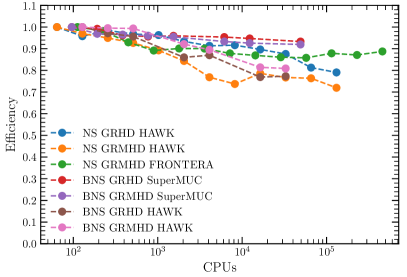
Figure 23: Weak scaling (Eq. (34)) for a single star and a binary neutron star configuration (NS and BNS, respectively) with and without magnetic fields (GRHD and GRMHD, respectively) for grids with SMR, comparing results on different target machines.

8 Conclusion

This paper presents an extension of GR-Athena++ that allows us to perform GRMHD simulations of astrophysical flows on dynamical spacetimes. The code implements 3+1 Eulerian GRMHD in conservative form and couples it to the Z4c metric solver presented in Daszuta et al. (2021). The MHD solver is a direct extension of Athena++’s constrained-transport scheme (Stone et al., 2020), implemented on an oct-tree mesh with block-based AMR. Other novel technical aspects introduced with respect to the original codebase are grid-to-grid operators between cell, vertex and face centered grid variables, WENO reconstruction schemes, a generic EOS interface and a new conservative-to-primitive solver.

The code is mainly targeted to astrophysical applications involving neutron star spacetimes. We have demonstrated it can successfully pass a standard set of challenging benchmarks, including the long-term stable evolution of isolated equilibrium neutron star configurations, the gravitational collapse of an unstable rotating neutron star to a black hole (and the subsequent black hole evolution), and binary neutron star mergers from inspiral to merger remnants. For the latter tests, we have demonstrated gravitational waveforms that are convergent and consistent with the BAM code. Notably, most of the performed tests involve no grid symmetries and rather low resolutions, while still providing quantitatively correct results.

Anticipating full-scale applications, we have discussed novel simulations of magnetic field instabilities in both isolated and merging neutron stars. We have performed long-term evolutions of isolated magnetised neutron stars with initially poloidal fields up to 68.7 ms extending our previous simulations in Sur et al. (2022) to include full dynamical spacetime evolution. Here we find similar results for the growth of a toroidal field component, saturating at approximately $10\%$ of the total magnetic field energy, while finding a superior conservation of the internal energy of the neutron star, and total relative violations of the divergence-free condition on the magnetic field of order $10^{-16}$.

We have also performed mergers of magnetised binary neutron stars utilising the full AMR capabilities of Athena++ to efficiently resolve the Kelvin-Helmholtz instability, investigating the efficiency and performance of two refinement strategies based on dynamically evolving field values. Even at initially low resolutions we find an amplification of a factor $\sim{}8$ when refining by 1 extra level based on the magnitude of the magnetic field, while utilising a factor $\sim{}2$ fewer MeshBlocks at the moment of merger, compared to an SMR resolution of the same resolution at the NSs.

The scaling properties of GR-Athena++ have been tested on a variety of machines and for differing problems, with strong scaling efficiencies in excess of $80\%$ shown up to $10^{5}$ CPU cores, and weak scaling efficiency in excess of $90\%$ as far as our tests have extended, up to $\sim{}5\times 10^{4}$ CPU cores for a magnetised binary neutron star evolution. For a single star we also tested the scaling behaviour, with weak scaling holding at efficiencies of up to $89\%$ on $\sim{}5\times 10^{5}$ CPU cores. This scaling efficiency will allow us to tackle large GRMHD problems without symmetries.

Work is ongoing on further improving some algorithmic aspects and physics modules of GR-Athena++. A code version employing cell-centered metric fields and high-order restrict-prolong operators is also under testing. A future paper will report on a detailed comparison of the performances of vertex-centered and cell-centered metric representation for vacuum and neutron star spacetimes. For the computation of accurate gravitational waveforms we are implementing high-order schemes which have proven to be essential for waveform convergence and overall quality (Radice et al., 2014b; Bernuzzi & Dietrich, 2016; Doulis et al., 2022). Further, the accuracy of computations of merger remnants and other strong-gravity phenomena depends crucially on the detailed simulation of microphysics. To this aim, we are porting into GR-Athena++ the neutrino transport scheme developed by Radice et al. (2022) together with a physically improved implementation of weak reactions and reaction rates. We also plan to couple to GR-Athena++ the sophisticated radiation solvers recently developed in the Athena++ framework by Bhattacharyya & Radice (2022); White et al. (2023).

Appendix A PrimitiveSolver

PrimitiveSolver is a new conserved-to-primitive library based on the algorithm of Kastaun et al. (2021) (hereafter KKC). However, it implements a small number of changes.

First, temperature is treated as a fundamental thermodynamic variable over the specific internal energy, $\epsilon$. While the distinction is trivial for an ideal gas, this convention coincides better with the nuclear EOS tables commonly employed in core-collapse supernova and BNS simulations. In principle this also means that common thermodynamic expressions which require expensive root solves on tables can now be written as lookup operations, though in practice this is not always the case.

Secondly, internal PrimitiveSolver calculations use the total energy density $e=\rho(1+\epsilon)$ in place of $\epsilon$. This offers a small computational advantage, as the estimate of $e$ from the root solver, $\hat{e}$, requires fewer floating-point operations than the calculation of $\hat{\epsilon}$ as described by KKC, without any significant round-off error for velocities near zero. Certain intermediate calculations can also be carried through, resulting in approximately five fewer floating-point operations for a single root iteration.

PrimitiveSolver passes an extensive set of unit tests to demonstrate self-consistency between the primitive-to-conserved and conserved-to-primitive procedures, typically maintaining a relative error of $10^{-10}$ or less for all but the most extreme situations ($W\sim 10^{3}$ for an ideal gas, $W\sim 10^{2}$ for a tabulated EOS). We have additionally validated our implementation against the reference implementation of KKC in RePrimAnd in systematic benchmarks, and we find that our algorithmic changes do not result in any noticeable difference in accuracy. We also find that the root solver in PrimitiveSolver is more robust and often converges faster, particularly for large $W$, than RePrimAnd.

The most important difference between PrimitiveSolver and RePrimAnd, however, is architectural: the latter utilizes a more traditional polymorphic design, with each EOS inheriting from an abstract interface class and implementing specific EOS behavior through virtual functions. PrimitiveSolver instead uses a templated policy-based design; the base EOS interface accepts a specific equation of state as a template parameter and inherits directly from that class. While adding an element of complexity to the interface class, this change eliminates the need for virtual functions, which has benefits for vectorizing the code and porting it to other architectures, such as GPUs.

In addition to the EOS, PrimitiveSolver also templates over the error policy, which includes both the atmosphere treatment and responses to problems occurring during the primitive solve. The standard policy used in GR-Athena++ defines an atmosphere with $\rho=\rho_{\textrm{atm}}$, $T=T_{\textrm{atm}}$, and $v^{i}=0$. If either $\rho$ or $D$ falls below $\rho_{\textrm{atm}}f_{\textrm{thr}}$, where $f_{\textrm{thr}}$ is a thresholding coefficient, all hydrodynamical variables are reset to atmosphere. If $T$ falls below $T_{\textrm{atm}}$, $T$ is reset, and the pressure is recalculated. During the conserved-to-primitive inversion, a density and composition-dependent floor assuming $T=0$ is calculated for $\tau$. If $\tau$ falls below this value, it is reset, but all other variables are left untouched.

Because the GRMHD equations become ill-conditioned when $B^{2}/D\gg 1$ or $W\gg 1$, limits are imposed on these variables during the conserved-to-primitive inversion. If $B^{2}/D>M_{\textrm{max}}$, $D$ is rescaled to $B^{2}/M_{\textrm{max}}$. If $W>W_{\textrm{max}}$, $W$ is reset to $W_{\textrm{max}}$ without modifying the conserved variables, effectively increasing $\rho$.

Lastly, during the root solve step for the inversion procedure, it can happen that the calculated values of $\rho$, $e$, or $T$ fall outside the bounds permitted by the EOS, particularly when using a tabulated EOS. In these circumstances, the quantity is simply reset to the nearest permissible value.

References

- Abbott et al. (2017a) Abbott, B. P., et al. 2017a, Phys. Rev. Lett., 119, 161101, doi: 10.1103/PhysRevLett.119.161101
- Abbott et al. (2017b) —. 2017b, Astrophys. J., 848, L13, doi: 10.3847/2041-8213/aa920c
- Abbott et al. (2017c) —. 2017c, Astrophys. J., 848, L12, doi: 10.3847/2041-8213/aa91c9
- Aguilera-Miret et al. (2023) Aguilera-Miret, R., Palenzuela, C., Carrasco, F., & Viganò, D. 2023. https://arxiv.org/abs/2307.04837
- Alcubierre et al. (2000) Alcubierre, M., Brandt, S., Bruegmann, B., et al. 2000, Class. Quant. Grav., 17, 2159, doi: 10.1088/0264-9381/17/11/301
- Alic et al. (2012) Alic, D., Bona-Casas, C., Bona, C., Rezzolla, L., & Palenzuela, C. 2012, Phys.Rev., D85, 064040, doi: 10.1103/PhysRevD.85.064040
- Alic et al. (2013) Alic, D., Kastaun, W., & Rezzolla, L. 2013, Phys. Rev., D88, 064049, doi: 10.1103/PhysRevD.88.064049
- Anderson et al. (2006) Anderson, M., Hirschmann, E., Liebling, S. L., & Neilsen, D. 2006, Class.Quant.Grav., 23, 6503, doi: 10.1088/0264-9381/23/22/025
- Anderson et al. (2008) Anderson, M., Hirschmann, E. W., Lehner, L., et al. 2008, Phys.Rev., D77, 024006, doi: 10.1103/PhysRevD.77.024006
- Anile (1990) Anile, A. M. 1990, Relativistic Fluids and Magneto-fluids
- Anninos et al. (2005) Anninos, P., Fragile, P. C., & Salmonson, J. D. 2005, Astrophys. J., 635, 723, doi: 10.1086/497294
- Anton et al. (2006) Anton, L., Zanotti, O., Miralles, J. A., et al. 2006, Astrophys.J., 637, 296, doi: 10.1086/498238
- Arcavi et al. (2017) Arcavi, I., et al. 2017, Nature, 551, 64, doi: 10.1038/nature24291
- Baiotti et al. (2009) Baiotti, L., Bernuzzi, S., Corvino, G., De Pietri, R., & Nagar, A. 2009, Phys. Rev., D79, 024002, doi: 10.1103/PhysRevD.79.024002
- Baiotti et al. (2005) Baiotti, L., Hawke, I., Montero, P. J., et al. 2005, Phys.Rev., D71, 024035, doi: 10.1103/PhysRevD.71.024035
- Baker et al. (2006) Baker, J. G., Centrella, J., Choi, D.-I., Koppitz, M., & van Meter, J. 2006, Phys. Rev. Lett., 96, 111102, doi: 10.1103/PhysRevLett.96.111102
- Balbus & Hawley (1991) Balbus, S. A., & Hawley, J. F. 1991, ApJ, 376, 214, doi: 10.1086/170270
- Balsara (1998) Balsara, D. S. 1998, ApJS, 116, 133, doi: 10.1086/313093
- Banyuls et al. (1997) Banyuls, F., Font, J. A., Ibanez, J. M. A., Marti, J. M. A., & Miralles, J. A. 1997, Astrophys. J., 476, 221
- Baumgarte & Shapiro (1999) Baumgarte, T. W., & Shapiro, S. L. 1999, Phys. Rev., D59, 024007, doi: 10.1103/PhysRevD.59.024007
- Beckwith & Stone (2011) Beckwith, K., & Stone, J. M. 2011, Astrophys. J. Suppl., 193, 6, doi: 10.1088/0067-0049/193/1/6
- Bernuzzi & Dietrich (2016) Bernuzzi, S., & Dietrich, T. 2016, Phys. Rev., D94, 064062, doi: 10.1103/PhysRevD.94.064062
- Bernuzzi & Hilditch (2010) Bernuzzi, S., & Hilditch, D. 2010, Phys. Rev., D81, 084003, doi: 10.1103/PhysRevD.81.084003
- Bernuzzi et al. (2012) Bernuzzi, S., Nagar, A., Thierfelder, M., & Brügmann, B. 2012, Phys.Rev., D86, 044030, doi: 10.1103/PhysRevD.86.044030
- Bernuzzi et al. (2020) Bernuzzi, S., et al. 2020, Mon. Not. Roy. Astron. Soc., doi: 10.1093/mnras/staa1860
- Bhattacharyya & Radice (2022) Bhattacharyya, M. K., & Radice, D. 2022, doi: 10.1016/j.jcp.2023.112365
- Blinnikov et al. (1984) Blinnikov, S. I., Novikov, I. D., Perevodchikova, T. V., & Polnarev, A. G. 1984, Soviet Astronomy Letters, 10, 177, doi: 10.48550/arXiv.1808.05287
- Borges et al. (2008) Borges, R., Carmona, M., Costa, B., & Don, W. S. 2008, Journal of Computational Physics, 227, 3191, doi: 10.1016/j.jcp.2007.11.038
- Braithwaite & Spruit (2006) Braithwaite, J., & Spruit, H. C. 2006, Astron. Astrophys., 450, 1097, doi: 10.1051/0004-6361:20041981
- Brandt & Brügmann (1997) Brandt, S., & Brügmann, B. 1997, Phys. Rev. Lett., 78, 3606, doi: 10.1103/PhysRevLett.78.3606
- Brügmann (1996) Brügmann, B. 1996, Phys. Rev., D54, 7361, doi: 10.1103/PhysRevD.54.7361
- Brügmann et al. (2008) Brügmann, B., Gonzalez, J. A., Hannam, M., et al. 2008, Phys.Rev., D77, 024027, doi: 10.1103/PhysRevD.77.024027
- Campanelli et al. (2006) Campanelli, M., Lousto, C. O., Marronetti, P., & Zlochower, Y. 2006, Phys. Rev. Lett., 96, 111101, doi: 10.1103/PhysRevLett.96.111101
- Cheong et al. (2021) Cheong, P. C.-K., Lam, A. T.-L., Ng, H. H.-Y., & Li, T. G. F. 2021, Mon. Not. Roy. Astron. Soc., 508, 2279, doi: 10.1093/mnras/stab2606
- Christodoulou (1970) Christodoulou, D. 1970, Phys. Rev. Lett., 25, 1596, doi: 10.1103/PhysRevLett.25.1596
- Ciolfi (2018) Ciolfi, R. 2018, Int. J. Mod. Phys. D, 27, 1842004, doi: 10.1142/S021827181842004X
- Ciolfi et al. (2011) Ciolfi, R., Lander, S. K., Manca, G. M., & Rezzolla, L. 2011, Astrophys.J., 736, L6, doi: 10.1088/2041-8205/736/1/L6
- Ciolfi & Rezzolla (2013) Ciolfi, R., & Rezzolla, L. 2013, Mon. Not. Roy. Astron. Soc., 435, L43, doi: 10.1093/mnrasl/slt092
- Cipolletta et al. (2020) Cipolletta, F., Kalinani, J. V., Giacomazzo, B., & Ciolfi, R. 2020, Class. Quant. Grav., 37, 135010, doi: 10.1088/1361-6382/ab8be8
- Colella et al. (2011) Colella, P., Dorr, M. R., Hittinger, J. A. F., & Martin, D. F. 2011, Journal of Computational Physics, 230, 2952, doi: 10.1016/j.jcp.2010.12.044
- Combi & Siegel (2023a) Combi, L., & Siegel, D. M. 2023a, Astrophys. J., 944, 28, doi: 10.3847/1538-4357/acac29
- Combi & Siegel (2023b) —. 2023b. https://arxiv.org/abs/2303.12284
- Coulter et al. (2017) Coulter, D. A., et al. 2017, Science, doi: 10.1126/science.aap9811
- Curtis et al. (2022) Curtis, S., Mösta, P., Wu, Z., et al. 2022, Mon. Not. Roy. Astron. Soc., 518, 5313, doi: 10.1093/mnras/stac3128
- Damour et al. (2012) Damour, T., Nagar, A., Pollney, D., & Reisswig, C. 2012, Phys.Rev.Lett., 108, 131101, doi: 10.1103/PhysRevLett.108.131101
- Daszuta et al. (2021) Daszuta, B., Zappa, F., Cook, W., et al. 2021, Astrophys. J. Supp., 257, 25, doi: 10.3847/1538-4365/ac157b
- de Haas et al. (2022) de Haas, S., Bosch, P., Mösta, P., Curtis, S., & Schut, N. 2022. https://arxiv.org/abs/2208.05330
- Dedner et al. (2002) Dedner, A., Kemm, F., Kröner, D., et al. 2002, Journal of Computational Physics, 175, 645, doi: 10.1006/jcph.2001.6961
- Del Zanna et al. (2007) Del Zanna, L., Zanotti, O., Bucciantini, N., & Londrillo, P. 2007, Astron. Astrophys., 473, 11, doi: 10.1051/0004-6361:20077093
- Dietrich & Bernuzzi (2015) Dietrich, T., & Bernuzzi, S. 2015, Phys.Rev., D91, 044039, doi: 10.1103/PhysRevD.91.044039
- Dimmelmeier et al. (2006) Dimmelmeier, H., Stergioulas, N., & Font, J. A. 2006, Mon. Not. Roy. Astron. Soc., 368, 1609, doi: 10.1111/j.1365-2966.2006.10274.x
- Doulis et al. (2022) Doulis, G., Atteneder, F., Bernuzzi, S., & Brügmann, B. 2022, Phys. Rev. D, 106, 024001, doi: 10.1103/PhysRevD.106.024001
- Duez et al. (2008) Duez, M. D., Foucart, F., Kidder, L. E., et al. 2008, Phys. Rev., D78, 104015, doi: 10.1103/PhysRevD.78.104015
- Duez et al. (2005) Duez, M. D., Liu, Y. T., Shapiro, S. L., & Stephens, B. C. 2005, Phys. Rev., D72, 024028, doi: 10.1103/PhysRevD.72.024028
- Duez et al. (2003) Duez, M. D., Marronetti, P., Shapiro, S. L., & Baumgarte, T. W. 2003, Phys. Rev., D67, 024004, doi: 10.1103/PhysRevD.67.024004
- East et al. (2012) East, W. E., Pretorius, F., & Stephens, B. C. 2012, Phys.Rev., D85, 124010, doi: 10.1103/PhysRevD.85.124010
- Eichler et al. (1989) Eichler, D., Livio, M., Piran, T., & Schramm, D. N. 1989, Nature, 340, 126, doi: 10.1038/340126a0
- Endrizzi et al. (2020) Endrizzi, A., Perego, A., Fabbri, F. M., et al. 2020, Eur. Phys. J. A, 56, 15, doi: 10.1140/epja/s10050-019-00018-6
- Etienne et al. (2010) Etienne, Z. B., Liu, Y. T., & Shapiro, S. L. 2010, Phys. Rev., D82, 084031, doi: 10.1103/PhysRevD.82.084031
- Etienne et al. (2015) Etienne, Z. B., Paschalidis, V., Haas, R., Mösta, P., & Shapiro, S. L. 2015, Class. Quant. Grav., 32, 175009, doi: 10.1088/0264-9381/32/17/175009
- Etienne et al. (2012) Etienne, Z. B., Paschalidis, V., Liu, Y. T., & Shapiro, S. L. 2012, Phys.Rev., D85, 024013, doi: 10.1103/PhysRevD.85.024013
- Evans & Hawley (1988) Evans, C. R., & Hawley, J. F. 1988, Astrophys. J., 332, 659, doi: 10.1086/166684
- Flowers & Ruderman (1977) Flowers, E., & Ruderman, M. A. 1977, ApJ, 215, 302, doi: 10.1086/155359
- Font (2007) Font, J. A. 2007, Living Rev. Rel., 11, 7
- Font et al. (2000) Font, J. A., Miller, M. A., Suen, W.-M., & Tobias, M. 2000, Phys. Rev., D61, 044011
- Font et al. (2002) Font, J. A., et al. 2002, Phys. Rev., D65, 084024, doi: 10.1103/PhysRevD.65.084024
- Foucart et al. (2011) Foucart, F., Duez, M. D., Kidder, L. E., & Teukolsky, S. A. 2011, Phys. Rev., D83, 024005, doi: 10.1103/PhysRevD.83.024005
- Gammie et al. (2003) Gammie, C. F., McKinney, J. C., & Toth, G. 2003, Astrophys.J., 589, 444, doi: 10.1086/374594
- Gardiner & Stone (2005) Gardiner, T. A., & Stone, J. M. 2005, Journal of Computational Physics, 205, 509, doi: 10.1016/j.jcp.2004.11.016
- Gardiner & Stone (2008) Gardiner, T. A., & Stone, J. M. 2008, J. Comput. Phys., 227, 4123, doi: 10.1016/j.jcp.2007.12.017
- Giacomazzo & Rezzolla (2007) Giacomazzo, B., & Rezzolla, L. 2007, Class. Quant. Grav., 24, S235, doi: 10.1088/0264-9381/24/12/S16
- Goldberg et al. (1967) Goldberg, J. N., MacFarlane, A. J., Newman, E. T., Rohrlich, F., & Sudarshan, E. C. G. 1967, J. Math. Phys., 8, 2155
- Goldstein et al. (2017) Goldstein, A., et al. 2017, Astrophys. J., 848, L14, doi: 10.3847/2041-8213/aa8f41
- Goodman (1986) Goodman, J. 1986, ApJ, 308, L47, doi: 10.1086/184741
- Gourgoulhon et al. (2001) Gourgoulhon, E., Grandclement, P., Taniguchi, K., Marck, J.-A., & Bonazzola, S. 2001, Phys.Rev., D63, 064029, doi: 10.1103/PhysRevD.63.064029
- Guercilena et al. (2017) Guercilena, F., Radice, D., & Rezzolla, L. 2017, Comput. Astrophys. Cosmol., 4, 3, doi: 10.1186/s40668-017-0022-0
- Gundlach (1998) Gundlach, C. 1998, Phys. Rev. D, 57, 863, doi: 10.1103/PhysRevD.57.863
- Gundlach & Leveque (2011) Gundlach, C., & Leveque, R. J. 2011, J. Fluid Mech., 676, 237, doi: 10.1017/jfm.2011.42
- Hammond et al. (2021) Hammond, P., Hawke, I., & Andersson, N. 2021, Phys. Rev. D, 104, 103006, doi: 10.1103/PhysRevD.104.103006
- Hilditch et al. (2013) Hilditch, D., Bernuzzi, S., Thierfelder, M., et al. 2013, Phys. Rev., D88, 084057, doi: 10.1103/PhysRevD.88.084057
- Jiang & Shu (1996) Jiang, G.-S., & Shu, C.-W. 1996, Journal of Computational Physics, 126, 202, doi: 10.1006/jcph.1996.0130
- Kasen et al. (2017) Kasen, D., Metzger, B., Barnes, J., Quataert, E., & Ramirez-Ruiz, E. 2017, Nature, doi: 10.1038/nature24453
- Kastaun (2006) Kastaun, W. 2006, Phys. Rev. D, 74, 124024, doi: 10.1103/PhysRevD.74.124024
- Kastaun et al. (2021) Kastaun, W., Kalinani, J. V., & Ciolfi, R. 2021, Phys. Rev. D, 103, 023018, doi: 10.1103/PhysRevD.103.023018
- Kidder et al. (2017) Kidder, L. E., et al. 2017, J. Comput. Phys., 335, 84, doi: 10.1016/j.jcp.2016.12.059
- Kiuchi et al. (2015) Kiuchi, K., Cerdá-Durán, P., Kyutoku, K., Sekiguchi, Y., & Shibata, M. 2015, Phys. Rev. D, 92, 124034, doi: 10.1103/PhysRevD.92.124034
- Kiuchi et al. (2022) Kiuchi, K., Fujibayashi, S., Hayashi, K., et al. 2022. https://arxiv.org/abs/2211.07637
- Kiuchi et al. (2018) Kiuchi, K., Kyutoku, K., Sekiguchi, Y., & Shibata, M. 2018, Phys. Rev., D97, 124039, doi: 10.1103/PhysRevD.97.124039
- Kiuchi et al. (2014) Kiuchi, K., Kyutoku, K., Sekiguchi, Y., Shibata, M., & Wada, T. 2014, Phys.Rev., D90, 041502, doi: 10.1103/PhysRevD.90.041502
- Kiuchi et al. (2008) Kiuchi, K., Shibata, M., & Yoshida, S. 2008, Phys. Rev., D78, 024029, doi: 10.1103/PhysRevD.78.024029
- Komissarov (1999) Komissarov, S. S. 1999, Mon. Not. Roy. Astron. Soc., 303, 343, doi: 10.1046/j.1365-8711.1999.02244.x
- Komissarov (2005) Komissarov, S. S. 2005, Mon. Not. Roy. Astron. Soc., 359, 801, doi: 10.1111/j.1365-2966.2005.08974.x
- Kulkarni (2005) Kulkarni, S. R. 2005. https://arxiv.org/abs/astro-ph/0510256
- Kumar & Zhang (2014) Kumar, P., & Zhang, B. 2014, Phys. Rept., 561, 1, doi: 10.1016/j.physrep.2014.09.008
- Lasky et al. (2011) Lasky, P. D., Zink, B., Kokkotas, K. D., & Glampedakis, K. 2011, Astrophys. J. Lett., 735, L20, doi: 10.1088/2041-8205/735/1/L20
- Li & Paczynski (1998) Li, L.-X., & Paczynski, B. 1998, Astrophys.J., 507, L59, doi: 10.1086/311680
- Liebling et al. (2010) Liebling, S. L., Lehner, L., Neilsen, D., & Palenzuela, C. 2010, Phys. Rev., D81, 124023, doi: 10.1103/PhysRevD.81.124023
- Liu et al. (1994) Liu, X.-D., Osher, S., & Chan, T. 1994, Journal of Computational Physics, 115, 200 , doi: http://dx.doi.org/10.1006/jcph.1994.1187
- Liu et al. (2008) Liu, Y. T., Shapiro, S. L., Etienne, Z. B., & Taniguchi, K. 2008, Phys. Rev., D78, 024012, doi: 10.1103/PhysRevD.78.024012
- Löffler et al. (2012) Löffler, F., et al. 2012, Class. Quant. Grav., 29, 115001, doi: 10.1088/0264-9381/29/11/115001
- Londrillo & Del Zanna (2004) Londrillo, P., & Del Zanna, L. 2004, J.Comput.Phys., 195, 17, doi: 10.1016/j.jcp.2003.09.016
- Markey & Tayler (1973) Markey, P., & Tayler, R. J. 1973, MNRAS, 163, 77, doi: 10.1093/mnras/163.1.77
- Markey & Tayler (1974) —. 1974, MNRAS, 168, 505, doi: 10.1093/mnras/168.3.505
- Marti et al. (1991) Marti, J. M., Ibanez, J. M., & Miralles, J. A. 1991, Phys. Rev., D43, 3794, doi: 10.1103/PhysRevD.43.3794
- McCorquodale et al. (2015) McCorquodale, P., Dorr, M. R., Hittinger, J. A. F., & Colella, P. 2015, Journal of Computational Physics, 288, 181, doi: 10.1016/j.jcp.2015.01.006
- Metzger et al. (2010) Metzger, B., Martinez-Pinedo, G., Darbha, S., et al. 2010, Mon.Not.Roy.Astron.Soc., 406, 2650, doi: 10.1111/j.1365-2966.2010.16864.x
- Mösta et al. (2014) Mösta, P., Mundim, B. C., Faber, J. A., et al. 2014, Class.Quant.Grav., 31, 015005, doi: 10.1088/0264-9381/31/1/015005
- Mösta et al. (2020) Mösta, P., Radice, D., Haas, R., Schnetter, E., & Bernuzzi, S. 2020, Astrophys. J. Lett., 901, L37, doi: 10.3847/2041-8213/abb6ef
- Narayan et al. (1992) Narayan, R., Paczynski, B., & Piran, T. 1992, Astrophys. J., 395, L83. https://arxiv.org/abs/astro-ph/9204001
- Paczynski (1986) Paczynski, B. 1986, Astrophys. J., 308, L43
- Palenzuela et al. (2022) Palenzuela, C., Aguilera-Miret, R., Carrasco, F., et al. 2022, Phys. Rev. D, 106, 023013, doi: 10.1103/PhysRevD.106.023013
- Palenzuela et al. (2018) Palenzuela, C., Miñano, B., Viganò, D., et al. 2018, Class. Quant. Grav., 35, 185007, doi: 10.1088/1361-6382/aad7f6
- Perego et al. (2019) Perego, A., Bernuzzi, S., & Radice, D. 2019, Eur. Phys. J., A55, 124, doi: 10.1140/epja/i2019-12810-7
- Pian et al. (2017) Pian, E., et al. 2017, Nature, doi: 10.1038/nature24298
- Pili et al. (2014) Pili, A. G., Bucciantini, N., & Del Zanna, L. 2014, Mon. Not. Roy. Astron. Soc., 439, 3541, doi: 10.1093/mnras/stu215
- Pili et al. (2017) —. 2017, Mon. Not. Roy. Astron. Soc., 470, 2469, doi: 10.1093/mnras/stx1176
- Piran (2004) Piran, T. 2004, Rev. Mod. Phys., 76, 1143, doi: 10.1103/RevModPhys.76.1143
- Plewa & Mueller (1999) Plewa, T., & Mueller, E. 1999, Astron. Astrophys., 342, 179. https://arxiv.org/abs/astro-ph/9807241
- Pons & Viganò (2019) Pons, J. A., & Viganò, D. 2019, doi: 10.1007/s41115-019-0006-7
- Prakash et al. (2021) Prakash, A., Radice, D., Logoteta, D., et al. 2021, Phys. Rev. D, 104, 083029, doi: 10.1103/PhysRevD.104.083029
- Pretorius (2005a) Pretorius, F. 2005a, Class.Quant.Grav., 22, 425, doi: 10.1088/0264-9381/22/2/014
- Pretorius (2005b) —. 2005b, Phys. Rev. Lett., 95, 121101, doi: 10.1103/PhysRevLett.95.121101
- Price & Rosswog (2006) Price, D., & Rosswog, S. 2006, Science, 312, 719, doi: 10.1126/science.1125201
- Radice et al. (2022) Radice, D., Bernuzzi, S., Perego, A., & Haas, R. 2022, Mon. Not. Roy. Astron. Soc., 512, 1499, doi: 10.1093/mnras/stac589
- Radice et al. (2018) Radice, D., Perego, A., Hotokezaka, K., et al. 2018, Astrophys. J., 869, 130, doi: 10.3847/1538-4357/aaf054
- Radice et al. (2014a) Radice, D., Rezzolla, L., & Galeazzi, F. 2014a, Class.Quant.Grav., 31, 075012, doi: 10.1088/0264-9381/31/7/075012
- Radice et al. (2014b) —. 2014b, Mon.Not.Roy.Astron.Soc., 437, L46, doi: 10.1093/mnrasl/slt137
- Rasio & Shapiro (1999) Rasio, F. A., & Shapiro, S. L. 1999, Classical and Quantum Gravity, 16, R1, doi: 10.1088/0264-9381/16/6/201
- Reisswig et al. (2013) Reisswig, C., Haas, R., Ott, C. D., et al. 2013, Phys. Rev., D87, 064023, doi: 10.1103/PhysRevD.87.064023
- Rosswog & Diener (2021) Rosswog, S., & Diener, P. 2021, Class. Quant. Grav., 38, 115002, doi: 10.1088/1361-6382/abee65
- Ruiz et al. (2011) Ruiz, M., Hilditch, D., & Bernuzzi, S. 2011, Phys. Rev., D83, 024025, doi: 10.1103/PhysRevD.83.024025
- Ryu et al. (1998) Ryu, D., Miniati, F., Jones, T. W., & Frank, A. 1998, Astrophys. J., 509, 244, doi: 10.1086/306481
- Savchenko et al. (2017) Savchenko, V., et al. 2017, Astrophys. J., 848, L15, doi: 10.3847/2041-8213/aa8f94
- Shankar et al. (2023) Shankar, S., Mösta, P., Brandt, S. R., et al. 2023, Class. Quant. Grav., 40, 205009, doi: 10.1088/1361-6382/acf2d9
- Shibata (1999) Shibata, M. 1999, Phys. Rev., D60, 104052, doi: 10.1103/PhysRevD.60.104052
- Shibata & Nakamura (1995) Shibata, M., & Nakamura, T. 1995, Phys. Rev., D52, 5428, doi: 10.1103/PhysRevD.52.5428
- Shibata & Sekiguchi (2005) Shibata, M., & Sekiguchi, Y.-i. 2005, Phys. Rev., D72, 044014, doi: 10.1103/PhysRevD.72.044014
- Shibata & Uryu (2000) Shibata, M., & Uryu, K. 2000, Phys. Rev., D61, 064001, doi: 10.1103/PhysRevD.61.064001
- Siegel et al. (2014) Siegel, D. M., Ciolfi, R., & Rezzolla, L. 2014, Astrophys. J., 785, L6, doi: 10.1088/2041-8205/785/1/L6
- Siegel & Metzger (2017) Siegel, D. M., & Metzger, B. D. 2017, Phys. Rev. Lett., 119, 231102, doi: 10.1103/PhysRevLett.119.231102
- Siegel et al. (2018) Siegel, D. M., Mösta, P., Desai, D., & Wu, S. 2018, Astrophys. J., 859, 71, doi: 10.3847/1538-4357/aabcc5
- Soares-Santos et al. (2017) Soares-Santos, M., et al. 2017, Astrophys. J., 848, L16, doi: 10.3847/2041-8213/aa9059
- Steiner et al. (2013) Steiner, A. W., Hempel, M., & Fischer, T. 2013, Astrophys. J., 774, 17, doi: 10.1088/0004-637X/774/1/17
- Stergioulas & Friedman (1995) Stergioulas, N., & Friedman, J. L. 1995, Astrophys. J., 444, 306, doi: 10.1086/175605
- Stone et al. (2008) Stone, J. M., Gardiner, T. A., Teuben, P., Hawley, J. F., & Simon, J. B. 2008, Astrophys. J. Suppl., 178, 137, doi: 10.1086/588755
- Stone et al. (2020) Stone, J. M., Tomida, K., White, C. J., & Felker, K. G. 2020, Astrophys. J. Suppl., 249, 4, doi: 10.3847/1538-4365/ab929b
- Sur et al. (2022) Sur, A., Cook, W., Radice, D., Haskell, B., & Bernuzzi, S. 2022, Mon. Not. Roy. Astron. Soc., 511, 3983, doi: 10.1093/mnras/stac353
- Tayler (1957) Tayler, R. J. 1957, Proceedings of the Physical Society B, 70, 31, doi: 10.1088/0370-1301/70/1/306
- Tayler (1973) —. 1973, MNRAS, 161, 365, doi: 10.1093/mnras/161.4.365
- Thierfelder et al. (2011a) Thierfelder, M., Bernuzzi, S., & Brügmann, B. 2011a, Phys.Rev., D84, 044012, doi: 10.1103/PhysRevD.84.044012
- Thierfelder et al. (2011b) Thierfelder, M., Bernuzzi, S., Hilditch, D., Brügmann, B., & Rezzolla, L. 2011b, Phys.Rev., D83, 064022, doi: 10.1103/PhysRevD.83.064022
- Tóth & Roe (2002) Tóth, G., & Roe, P. L. 2002, Journal of Computational Physics, 180, 736, doi: 10.1006/jcph.2002.7120
- Typel et al. (2015) Typel, S., Oertel, M., & Klähn, T. 2015, Phys. Part. Nucl., 46, 633, doi: 10.1134/S1063779615040061
- Tóth (2000) Tóth, G. 2000, Journal of Computational Physics, 161, 605 , doi: 10.1006/jcph.2000.6519
- van Leer (1974) van Leer, B. 1974, Journal of Computational Physics, 14, 361, doi: 10.1016/0021-9991(74)90019-9
- Viganò et al. (2018) Viganò, D., Martínez-Gómez, D., Pons, J. A., et al. 2018, doi: 10.1016/j.cpc.2018.11.022
- Weyhausen et al. (2012) Weyhausen, A., Bernuzzi, S., & Hilditch, D. 2012, Phys. Rev., D85, 024038, doi: 10.1103/PhysRevD.85.024038
- White et al. (2023) White, C. J., Mullen, P. D., Jiang, Y.-F., et al. 2023, Astrophys. J., 949, 103, doi: 10.3847/1538-4357/acc8cf
- White et al. (2016) White, C. J., Stone, J. M., & Gammie, C. F. 2016, Astrophys. J. Suppl., 225, 22, doi: 10.3847/0067-0049/225/2/22
- Wright (1973) Wright, G. A. E. 1973, MNRAS, 162, 339, doi: 10.1093/mnras/162.4.339