Deep Hashing via Householder Quantization

Abstract

Hashing is at the heart of large-scale image similarity search, and recent methods have been substantially improved through deep learning techniques. Such algorithms typically learn continuous embeddings of the data. To avoid a subsequent costly binarization step, a common solution is to employ loss functions that combine a similarity learning term (to ensure similar images are grouped to nearby embeddings) and a quantization penalty term (to ensure that the embedding entries are close to binarized entries, e.g., , -1 or 1). Still, the interaction between these two terms can make learning harder and the embeddings worse. We propose an alternative quantization strategy that decomposes the learning problem in two stages: first, perform similarity learning over the embedding space with no quantization; second, find an optimal orthogonal transformation of the embeddings so each coordinate of the embedding is close to its sign, and then quantize the transformed embedding through the sign function. In the second step, we parametrize orthogonal transformations using Householder matrices to efficiently leverage stochastic gradient descent. Since similarity measures are usually invariant under orthogonal transformations, this quantization strategy comes at no cost in terms of performance. The resulting algorithm is unsupervised, fast, hyperparameter-free and can be run on top of any existing deep hashing or metric learning algorithm. We provide extensive experimental results showing that this approach leads to state-of-the-art performance on widely used image datasets, and, unlike other quantization strategies, brings consistent improvements in performance to existing deep hashing algorithms.

1 Introduction

With the massive growth of image databases [13, 39, 11, 28], there has been an increasing need for fast image retrieval methods. Traditionally, hashing has been employed to quickly perform approximate nearest neighbor search while retaining good retrieval quality. For example, Locality-Sensitive Hashing (LSH) [2, 17, 21] assigns compact binary hash codes to images such that similar items receive similar hash codes, so the search can be conducted over hashes rather than images. Still, LSH methods are agnostic to the nature of the underlying data, often leading to sub-optimal performance.

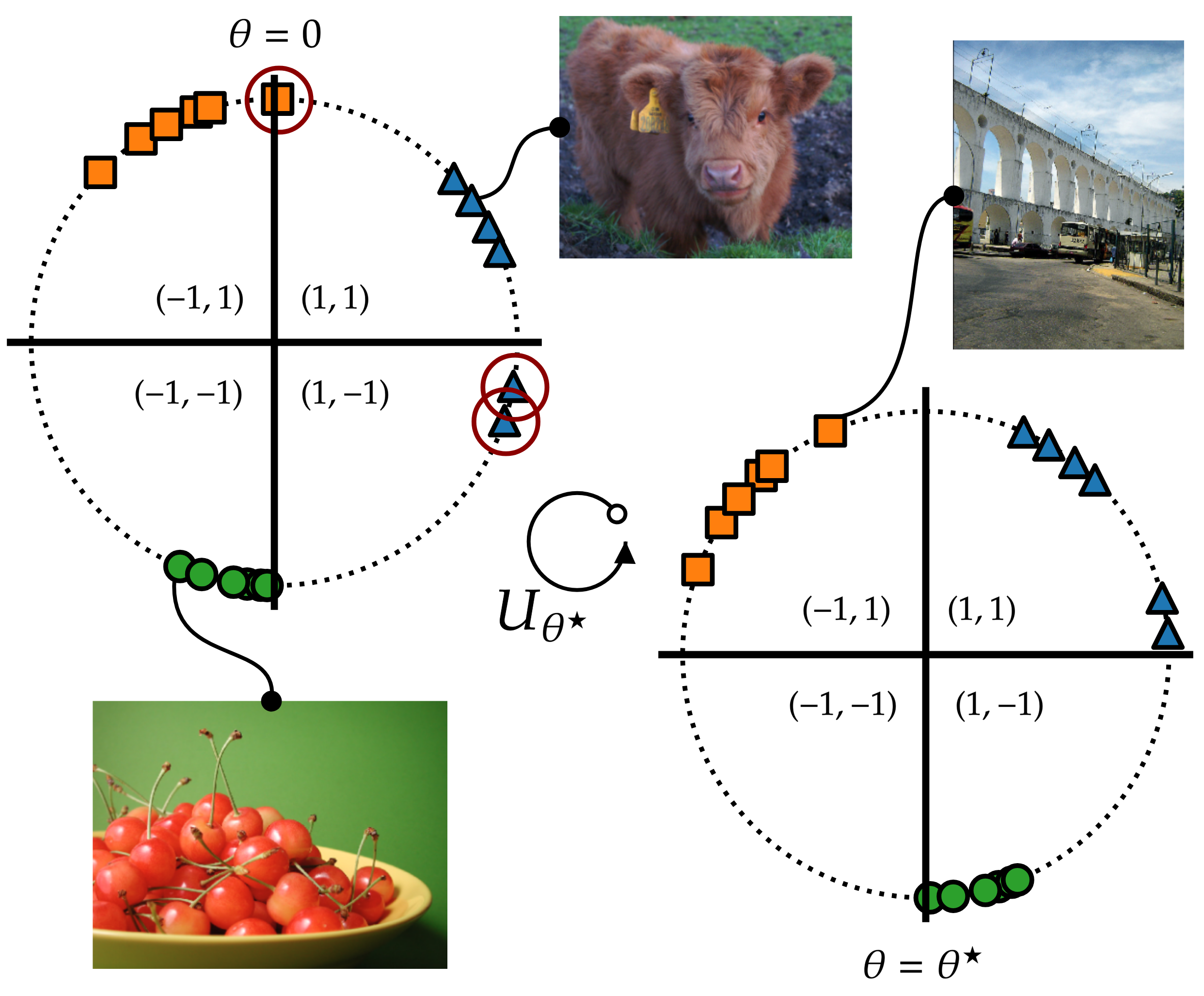
Figure 1: Deep hashing methods usually train low-dimensional embedding maps and obtain hashes by taking the sign of the embeddings coordinate-wise. To avoid a lossy discretization, a two-term loss $L=L_{S}+\lambda L_{Q}$ is used, where $L_{S}$ is a similarity term and $L_{Q}$ is a quantization term. In contrast, we first let $\lambda=0$, obtaining good similarity-preserving embeddings and then train an orthogonal transformation $U_{\theta}$ parametrized by $\theta\in\Theta$ to binarize the embedding via the coordinate-wise sign. As similarity losses are typically invariant under $U_{\theta}$, the term $L_{S}$ remains unchanged as an optimal discretization is found through the choice of $\theta$.

Indeed, many data-aware methods have recently been proposed, giving rise to the learning to hash literature [53] and substantially improving the results for the image retrieval problem. In unsupervised learning to hash [56, 54, 44, 42, 19], one uses only feature information (i.e., the image itself), while in supervised hashing [47, 43] one also employs additional available label information (e.g., a class the image belongs to) to capture semantic relationships between data points. With the significant advances brought about by deep learning in image tasks, deep hashing methods [45, 50] have become state-of-the-art methods in the field.

While hashing is discrete in nature, optimizing directly over binary hashes is usually intractable [55]. To overcome this, one alternative is to simply learn efficient embeddings through a similarity-learning term in the loss function, and then binarize the embedding (typically by using the coordinate-wise sign of the embedding, so they become either $-1$ or $1$). However, this quantization process can significantly decrease the retrieval quality, so most deep hashing methods try to account for it in the learning process. That is, deep hashing methods look for solutions such that (i) the learned embeddings preserve similarity well, which is solved through a similarity learning strategy; (ii) the error between the embedding and its binarized version is small, which calls for a quantization strategy. Most deep hashing methods combine the similarity learning and quantization strategies in a single two-termed loss function where one term accounts for similarity learning and the other term penalizes quantization error. As it turns out, the experiments in this paper show that learning similarity and quantization at the same time is often sub-optimal.

We propose to decouple the problem in two independent stages. First, we minimize the similarity term of the deep hashing method (e.g., , [59, 7, 6, 63, 36]) with no quantization penalty to obtain a continuous embedding for the images. Then, our quantization strategy consists in training a rotation (or, more generally an orthogonal transformation) that when applied to the previously obtained embeddings minimizes the distance between the embeddings and their binary discretization. Because similarity learning losses in deep hashing are invariant under rotations, this quantization strategy is effectively independent from the similarity step, so each step can be solved optimally.

More broadly, the process of optimizing an orthogonal transformation to reduce lossy compression from the quantization may be applied to any pre-trained embedding. We provide comprehensive experimental results to show that this two-step learning process significantly increases the performance metrics for most deep hashing methods, beating current state-of-the-art solutions, at a very low computation cost and with no hyperparameter tuning. In summary, our main contributions are:

• We propose a new quantization method called Householder hashing quantization (H²Q), which turns pre-trained embeddings into efficient hashes. The hash is created in two steps: (i) finding a good embedding of the data through some similarity learning strategy, and (ii) quantizing it after using optimal orthogonal transformations via Householder transforms (see Figure 1).

• While existing deep hashing methods often combine the two steps through a quantization term in the loss function, the strategy above typically yields better results by exploring an invariance in the similarity term to orthogonal transformations (see Section 3). Thus, for state-of-the-art hashing methods such as HyP², Householder quantization uniformly improves performance; this is not the case for other quantization strategies (see Sections 4.2 and 4.3).

• Our algorithm is unsupervised, fast and linear in the size of the data (Section 4.5). In contrast to most current quantization strategies, our method does not require hyperparameters. It can also be run atop any existing deep hashing or metric learning algorithm.

• In several experiments with NUS WIDE, MS COCO, CIFAR 10 and ImageNet datasets, we show that Householder quantization significantly helps the best performing hashing methods in the literature, delivering state-of-the-art results versus current benchmarks (Section 4.1).

2 Related Work

There is a vast literature on unsupervised hashing methods for image retrieval. An important early example is Locality-Sensitive Hashing [17, 2, 21], a data-agnostic framework that builds random hash functions such that similar images are mapped to similar hashes and so retrieval achieves sub-linear time complexity. Still, it is usually possible to build better hashes by learning the hash functions from the data under consideration, so many learning to hash methods have been proposed. For example, Spectral Hashing [56] and Semi-Supervised Hashing (SSH) [54] build on principal component analysis (PCA) to create data-aware embeddings which are then binarized using the sign function.

More recently, deep hashing methods have significantly advanced the state-of-the-art results for fast image retrieval. These methods compose the last layer of pre-trained convolutional neural network (CNN) architectures, such as AlexNet [30], VGG-11 and VGG-16 [48], with a sequence of fully connected layers to be fine-tuned. By using pre-trained architectures, they exploit the enriched features and start the training procedure with an embedding that already encodes a high level of semantic similarity between images. Convolutional Neural Network Hashing (CNNH) [57] was one of the first methods of this type; it first finds a binary encoding that approximates the similarity between data points, and then trains a CNN to map the original data points into this binary encoding. Deep Supervised Hashing (DSH) [41] considers a loss function with a similarity term which is analogous to the contrastive squared losses used in metric learning [32, 10] while adding a penalization term in terms of the $L_{1}$ loss. On the other hand, Deep Hashing Network (DHN) [63] considers a pairwise cross-entropy loss for the similarity term, while using the same $L_{1}$ quantization term. HashNet [7] builds on DHN by adding weights to counter the imbalance between the number of positive and negative paris, and also applies a hyperbolic tangent to the embedding to continuously approximate the sign function used in the binarization step. Deep Cauchy Hashing [6] and alternatives [51, 25, 37, 8] follow a similar strategy with variations on the choice of the similarity and penalization terms and the weights. Methods such as Pairwise Correlation Discrete Hashing (PCDH) [9] and Deep Supervised Discrete Hashing (DSDH) [38] additionally consider how well the hash codes can reconstruct available labels by using a classifier. An alternative to training with pairwise similarity losses is to use a triplet loss, as is the case for Deep Neural Networks Hashing (DNNH) [33]. Another alternative are proxy-based methods [20, 60, 16] such as OrthoHash [20] which maximizes the cosine similarity between data points and pre-defined target hash codes associated with each class. Fixing target hash codes might miss semantic relationships between class labels, so [3, 26] consider the hash centers as parameters to be learned. More recently, HyP²[58] combined a proxy-based loss with a pairwise similarity term, harnessing the power from both approaches to obtain state-of-the-art performance. This suggests that reducing quantization error through a penalty term is not a requirement for good performance in deep hashing methods.

Indeed, we build on these latest deep hashing methods by introducing a novel quantization strategy that exploits the gains in similarity learning at no cost in terms of quantization. It consists of efficiently binarizing the learned embeddings after applying an optimal orthogonal transformations obtained via stochastic gradient descent [46], based on a parametrization using Householder matrices. The orthogonal transformation is optimized to make the embedding entries as close to $-1,1$ as possible before the coordinate-wise sign function is applied. This approach is similar in spirit to other quantization strategies developed before deep hashing (e.g., , Iterative Quantization [19] and similar methods [22, 23, 55]), but with important differences. In [22], the authors propose using random orthogonal transformations to improve hash codes, and, in [23], the authors quantize database vectors with centroids using orthogonal Householder reflections. Both [19] and [55] propose iterative algorithms to learn orthogonal transformations under an $L_{2}$ loss. They iteratively solve an orthogonal Procrustes problem for fixed hash codes, and then find the binarized hash code given the orthogonal transformation found. More recently, HWSD [15] replaces each deep hashing method’s penalty term by a sliced Wasserstein distance. Our method differs from earlier rotation-based schemes [19, 22, 23, 55] since it is not iterative and exploits the capabilities of SGD to avoid spurious local minima; it also differs from HWSD because we do not jointly optimize embeddings and quantization. Furthermore, while previous quantization strategies sometimes degrade the embeddings learned by deep hashing algorithms, our proposed quantization strategy uniformly improves them (see Tables 1 and 2, and Figure 2).

3 Householder Hashing Quantization (H²Q)

In learning to hash, we are given a set of images $\{x_{i}\}_{i=1}^{n}$, $x_{i}\in\mathbb{R}^{d}$, and a notion of similarity between pairs of images $\mathcal{S}=(s_{ij})_{i,j\in[n]}$ taken to be $1$ for similar images (e.g., , from the same object or class) and $0$ for dissimilar ones. The goal is to learn a hash function $h_{\theta}:\mathbb{R}^{d}\mapsto\{-1,1\}^{k}$, with associated hash codes $b_{i}=h_{\theta}(x_{i})$, such that the Hamming distance $d_{H}(b_{i},b_{j})$ between $b_{i}$ and $b_{j}$,

$$d_{H}(b_{i},b_{j})=\sum_{l=1}^{k}\textbf{1}_{[b_{il}\neq b_{jl}]},$$

is small for similar pairs (i.e., , $s_{ij}=1$) and big for dissimilar ones ($s_{ij}=0$). Since optimizing over $b_{i}\in\{-1,1\}^{k}$ is computationally intractable [55], one usually learns a continuous embedding $f_{\theta}:\mathbb{R}^{d}\to\mathbb{R}^{k}$, with $\theta\in\Theta$ a parameter to be learned, and then binarize it via $h_{\theta}=\operatorname*{sign}\circ f_{\theta}$.

3.1 Deep Hashing Losses

In deep hashing, $\theta$ represents the weights of a neural network $f_{\theta}$, to be learned by stochastic gradient descent (SGD) using some loss function. Generally, one would like to directly optimize them in terms of $d_{ij}(\theta)=d_{H}(h_{\theta}(x_{i}),h_{\theta}(x_{j}))$, solving the minimization problem

$$\min_{\theta}\sum_{i,j}s_{ij}l_{S}(d_{ij}(\theta))+(1-s_{ij})l_{D}(d_{ij}(\theta)),$$ (3.1)

where $l_{S}$ and $l_{D}$ are losses for similar and dissimilar pairs of points, respectively. Many alternatives for $l_{S}$ and $l_{D}$ have been proposed (e.g., , [45, 53, 7, 6, 36, 63, 51, 59]).

However, due to the discrete nature of hash functions, the objective function in (3.1) is not differentiable in $\theta$. A common way to overcome this is to consider the identity:

$$\begin{split}d_{H}(b_{i},b_{j})&=\frac{k-\langle b_{i},b_{j}\rangle}{2}=\frac{k}{2}\left(1-\frac{\langle b_{i},b_{j}\rangle}{\|b_{i}\|_{2}\|b_{j}\|_{2}}\right),\end{split}$$ (3.2)

which holds when $b_{i},b_{j}\in\{-1,1\}^{k}$ are hash codes. This identity relates the Hamming distance with the inner product and the cosine similarity. By replacing $b_{i}$ and $b_{j}$ with $f_{i}=f_{\theta}(x_{i})$ and $f_{j}=f_{\theta}(x_{j})$ the last two expressions in (3.2) yield ways to measure the distance between pairs of points in the embedding, generalizing the Hamming distance to a differentiable expression. Thus, letting $\tilde{d}_{ij}(\theta)$ be either $(k-\langle f_{i},f_{j}\rangle)/2$ or $(k/2)\left(1-\langle f_{i},f_{j}\rangle/(\|f_{i}\|_{2}\|f_{j}\|_{2})\right)$, a relaxed version of (3.1) consists in minimizing the objective

$$L_{S}(\theta)=\sum_{i,j}s_{ij}l_{S}\left(\tilde{d}_{ij}(\theta)\right)+(1-s_{ij})l_{D}\left(\tilde{d}_{ij}(\theta)\right).$$ (3.3)

Once the embedding $f_{\theta}$ is learned, one typically binarizes it by taking its coordinate-wise sign (i.e., , $b(x_{i})=\operatorname*{sign}\circ f_{\theta}(x_{i})$), but this can be quite lossy when $f_{\theta}(x_{i})$ is very far from $\{-1,1\}^{k}$. To mitigate this effect, a penalty term is usually introduced to minimize the gap between $f_{i}$ and $b_{i}$. This gives rise to the two-term loss function:

$$L(\theta)=L_{S}(\theta)+\lambda\cdot L_{Q}(\theta),$$ (3.4)

where $L_{S}(\theta)$ takes the form in (3.3), $\lambda\in\mathbb{R}$ and a typical example of $L_{Q}(\theta)$ (e.g., , used in [36, 41, 61, 51]) would be:

$$L_{Q}(\theta)=\frac{1}{n}\sum_{i=1}^{n}\|f_{\theta}(x_{i})-h_{\theta}(x_{i})\|_{2}^{2},$$ (3.5)

Other quantization losses are explored in [63, 6]. Note, however, that this quantization strategy directly affects the learned embedding $f_{\theta}$ since (3.4) trains on both $L_{S}(\theta)$ and $\lambda\cdot L_{Q}(\theta)$, resulting in possibly subpar hashing performance.

3.2 The H²Q Quantization Procedure

We propose instead to decompose the similarity learning and the quantization strategies in two separate steps. First, for a given deep hashing method, set $\lambda=0$ in (3.4) and solve

$$\min_{\theta\in\Theta}L_{S}(\theta)$$ (3.6)

to learn an embedding $f_{\theta}$ that preserves similarity as well as possible. Then, normalize $f_{\theta}(x_{i})$ to obtain

$$\bar{f}_{\theta}(x_{i})=\sqrt{k}\frac{f_{\theta}(x_{i})}{\|f_{\theta}(x_{i})\|_{2}}$$

and, finally, solve the following optimization problem:

$$U^{\star}=\operatorname*{arg\,min}_{U\in O(k)}\frac{1}{n}\sum_{i=1}^{n}\left\|U\bar{f}_{\theta}(x_{i})-\operatorname*{sign}\left(U\bar{f}_{\theta}(x_{i})\right)\right\|_{2}^{2}.$$ (3.7)

Note this is minimizing a quantization error over the group $O(k)$ of orthogonal transformations in $\mathbb{R}^{k}$. We then obtain the final H²Q-quantized hash function $h_{\theta}=\operatorname*{sign}(U^{\star}f_{\theta})$.

Input: embeddings $f_{1},\dots,f_{n}\in\mathbb{R}^{k}$ of images $x_{1},\dots,x_{n}$ trained with a similarity-based loss (3.6).

Procedure

1. Compute $\bar{f_{i}}=\sqrt{k}\frac{f_{i}}{\|f_{i}\|_{2}}$ for $i=1,\ldots,n$;

2. Solve, using SGD,

   $$U^{\star}=\operatorname*{arg\,min}_{U\in O(k)}\frac{1}{n}\sum_{i=1}^{n}\left\|U\bar{f_{i}}-\operatorname*{sign}\left(U\bar{f}_{i}\right)\right\|_{2}^{2},$$

   where $O(k)$ is the orthogonal group parametrized

via Householder matrices (see Section 3.3);

Evaluate $h_{i}=\operatorname*{sign}(U^{\star}f_{i})\in\{-1,1\}^{k}$, $i=1,\ldots,n$; 4. Output hashes $h_{1},\ldots,h_{n}$ for images $x_{1},\ldots,x_{n}$.

Algorithm 1 H²Q quantization strategy.

Our proposed procedure is summarized in Algorithm 1. The normalization is required to avoid excessive penalization towards embeddings $f_{i}$ with larger norms $\|f_{i}\|_{2}$. Still, we note that, once $U^{\star}$ is found, the prediction can be done without normalization. The factor of $\sqrt{k}$ puts the normalized features in the Euclidean sphere containing the hash codes. Finally, the reason we use orthogonal transformations is due to the following result from linear algebra:

Theorem 3.1

A map $U:\mathbb{R}^{k}\mapsto\mathbb{R}^{k}$ preserves inner products if and only if it is a linear orthogonal transformation.

Proof:  See Appendix C in the Supplement.  $\Box$

Since cosine similarity depends only on inner products, it follows that orthogonal transformations also preserve cosine similarity between points. Thus, we are effectively optimizing our quantization strategy over the largest possible set of transformations that make the term $L_{S}$ invariant for the deep hashing. Hence, the quality of the embedding is not sacrificed due to the subsequent quantization.

3.3 Parametrizing Orthogonal Transformations

Finding the right parametrization of the orthogonal group $O(k)$ to solve (3.7) is non-trivial. One may consider, for example, matrix exponentials or Cayley maps [34, 1, 18, 35]. We propose to parametrize the elements of the group $O(k)$ as the product of Householder matrices. Geometrically, a Householder matrix is a reflection about a hyperplane with normal vector $v\in\mathbb{R}^{k}\setminus\{0\}$ and containing the origin, i.e., ,

$$H=I_{k}-2\frac{vv^{\intercal}}{\|v\|_{2}^{2}},$$ (3.8)

where $I_{k}\in\mathbb{R}^{k\times k}$ is the identity. Any orthogonal matrix can be decomposed as a product of Householder matrices:

Theorem 3.2

For every orthogonal matrix $U\in O(k)$, there exists vectors $v_{1},\dots,v_{k}\in\mathbb{R}^{k}\setminus\{0\}$ such that $U$ is the composition of their respective Householder matrices, i.e., ,

$$U=\prod_{i=1}^{k}\left(I_{k}-2\frac{v_{i}v_{i}^{\intercal}}{\|v_{i}\|^{2}}\right).$$ (3.9)

Conversely, every matrix with the form (3.9) is orthogonal.

Proof:  See Appendix C in the Supplement.  $\Box$

Thus, finding an optimal orthogonal transformation is equivalent to finding optimal $v_{1},\dots,v_{k}\in\mathbb{R}^{k}$, which can be thought of as parameters in (3.7), and learned through SGD. Since solving it using SGD requires several batch-evaluations of $U\bar{f_{i}}$, we use the matrix multiplication algorithm in [46] to perform this operation efficiently.

4 Experiments

In this section we present experimental evidence sustaining the following three claims:

1. H²Q is capable of improving state-of-the-art hashing, obtaining the best performance metrics over existing deep hashing alternatives;

2. H²Q always improves the metrics of cosine and inner-product similarity-based losses;

3. In contrast, other quantization strategies, such as ITQ [19], HWSD [15] and penalization terms (e.g., , (3.5)), may deteriorate performance, sometimes significantly.

Moreover, we also provide experiments regarding computational time and an ablation study where variants of (3.7) are discussed. We start by introducing our experimental setup.

Datasets. We consider four popular image retrieval datasets, of varying sizes: CIFAR 10 [29], NUS WIDE [12], MS COCO [40] and ImageNet [14].

CIFAR 10 [29] is an image dataset containing $60,000$ images divided into $10$ mutually exclusive classes. Following the literature [6, 63], we take $500$ images per class for the training set, $100$ images per class for the test and validation sets. The remaining images are used as database images.

NUS WIDE [12] is a web image dataset containing a total of $269,648$ images from flickr.com. Each image contains annotations from a set of 81 possible concepts. Following [59, 62], we first reduce the number of total images to $195,834$ by taking only images with at least one concept from the 21 most frequent ones. We then remove images that were unavailable for download from flickr.com, resulting in a set of $148,332$ images. From this subset we randomly sample $10,500$ images as training set and $2,100$ images for each of the query and validation sets. The remaining images compose our database, as in [59, 62].

MS COCO [40] is a dataset for image segmentation and captioning containing a total of $123,287$ images, $82,783$ from a training set and $40,500$ from a validation set. Each image has annotations from a list of $80$ semantic concepts. Following [6], we randomly sample $10,000$ images as training set, $5,000$ images for each of the query and validation set, and the remaining images are used as database images.

ImageNet [14] is a large image dataset with over $1,200,000$ images in the training set and $50,000$ in the validation set, each having a single label from a list of $1000$ possible categories. We use the same choice of $100$ categories as [7] resulting in the same training set, containing $13,000$ images, and database set, containing $128,503$ images. Finally, we split the $5,000$ images from the test set into $2,500$ images for each of the query and validation sets.

Evaluation metric. The standard metric in learning to hash is mean average precision [50]. It measures not only the precision of the retrieved items, but also the ranking in which the items are retrieved. More precisely, let $q$ be a query image and $D=\{x_{1},\dots,x_{n}\}$ be a database of images. Take $R(q)=(i_{1},i_{2},\dots,i_{n})$ to be a permutation of the indices $1,\dots,n$ corresponding to the sorting of images retrieved for the query $q$. Let $\delta(x;q)=1$ if $x$ is similar to $q$ and $\delta(x;q)=0$ otherwise. The average precision of the first $k\leq n$ entries in the permutation $R(q)$ is

$$AP_{k}(q)=\frac{\sum_{j=1}^{k}P(x_{i_{1}},\dots,x_{i_{j}};q)\delta(x_{i_{j}};q)}{\sum_{j=1}^{k}\delta(x_{i_{j}};q)}$$

where

$$P(x_{i_{1}},\dots,x_{i_{j}};q)=\frac{1}{j}\sum_{l=1}^{j}\delta(x_{i_{l}};q),$$

is the precision up to $j$. For a given set $Q$ of query points, the mean average precision at $k$ is then defined as

$$\texttt{mAP@k}=\frac{1}{|Q|}\sum_{q\in Q}AP_{k}(q).$$

We compute mAP@k with $k=1000$ for ImageNet and $k=5000$ for the remaining datasets, as is common in the field [7]. To evaluate a hashing scheme, we take $R(q)$ to be the ordering given by the Hamming distance between the hashes of $q$ and the hashes of the images in $D$ with ties broken using the cosine distance of the embeddings. High values of mAP@k imply most items returned in the first positions are similar to the query; thus, higher mAP@k is better.

Deep hashing benchmarks. To evaluate the performance of H²Q quantization, we consider its effect on six state-of-the-art benchmarks from the field: DPSH [36], DHN [63], HashNet [7], DCH [6], WGLHH [51], and HyP²[59]. The first three use similarity measures based on the inner product while the last three use cosine similarity. We also consider the classical Cosine Embedding Loss (CEL) [4], which is a classical metric learning algorithm. Each of these methods define a different loss function following (3.4) (see Section A.3 for details).

Quantization strategies. We compare how deep hashing benchmarks fare using the following strategies:

• no quantization, where we take $\lambda=0$ in (3.4);

• the original quantization penalty, which is obtained by taking $\lambda>0$ in (3.4) (see details on Section A.3);

• H²Q, as described in Algorithm 1;

• ITQ [19], where an orthogonal transformation is found through an iterative optimization process;

• HWSD [15], where the $L_{Q}$ term in (3.4) is replaced by their proposed quantization loss based on the sliced Wasserstein distance.

Neural network architectures. Following the learning to hash literature, we employed both AlexNet [31] and VGG-16 [49], and adapted the architectures by replacing the last fully connected layers with softmax by a single fully connected layer with no activation. The weights of the hashing layer were initialized following a centered normal with deviation $0.01$ and the bias initialized with zeros. The weights and bias of all other layers were initialized using the pre-trained weights from IMAGENET1K_V1 available on torchvision. Methods that use a quantization penalty (i.e., , $\lambda>0$ in (3.4)) require a final $\tanh$ activation layer constraining the embeddings to $(0,1)^{k}$ to enforce quantization.

H²Q Optimization. To solve (3.7), we optimize the objective function over $v_{1},\ldots,v_{k}\in\mathbb{R}^{k}$ using (3.9), which can be thought of as trainable vectors. We perform SGD using the Adam optimizer, employing the matrix multiplication algorithm in [46] to quickly evaluate $U\bar{f}_{i}$ in each batch.

Hyperparameters. Each benchmarks uses the recommended set of hyperparameters recommended by the respective authors (see Section A.3; when it is not available, they are picked using a validation set). For all methods, we used the Adam optimizer [27] with learning rate of $10^{-5}$ for all pre-trained layers and $10^{-4}$ for the hash layer. For every set of hyperparameters and quantization strategy, every method was run four times with different initializations; the final metric is the average of the four runs. We train the Householder transformation with the $L_{2}$ loss in (3.7) and a learning rate of $0.1$ using 300 epochs and a batch size of 128 (for other choices, see Section 4.4).

	CIFAR 10				NUS WIDE				MS COCO				ImageNet
number of bits ($k$)	16	32	48	64	16	32	48	64	16	32	48	64	16	32	48	64
ADSH	56.7	71.8	77.3	79.7	74.8	78.4	79.8	80.3	57.9	61.1	63.7	65.0	5.2	8.3	13.4	23.2
CEL	79.8	81.0	81.7	81.3	79.4	80.3	80.7	80.7	64.4	66.3	67.5	68.4	51.8	52.5	53.7	45.6
DHN	81.2	81.1	81.1	81.3	80.6	81.3	81.6	81.7	66.8	67.3	69.2	69.4	25.1	32.4	35.7	38.2
DCH	80.2	80.1	80.0	79.8	78.4	79.1	79.1	79.8	63.8	66.2	67.1	66.7	58.2	58.8	58.9	60.4
DPSH	81.2	81.2	81.5	81.1	81.0	81.9	82.1	82.1	68.0	71.2	71.6	72.4	36.5	42.2	46.0	49.9
HashNet	80.8	82.1	82.3	82.3	79.8	81.5	82.2	82.7	62.9	67.3	68.2	70.2	41.2	54.3	58.8	62.5
WGLHH	79.6	80.0	80.2	79.4	79.9	80.7	80.1	80.5	66.3	67.0	67.7	67.2	55.3	57.1	57.0	56.8
HyP²	80.5	81.1	81.7	81.8	81.9	82.5	83.1	83.0	71.9	74.1	74.8	74.9	54.1	56.9	57.7	56.5
HyP² + H²Q	82.3	82.5	82.9	83.1	82.5	83.2	83.4	83.3	73.9	75.4	75.9	75.7	57.3	60.7	61.5	60.6

Table 1: mAP@k of each benchmark over AlexNet, along with with H²Q improvement over HyP². Numbers in bold indicate that best metric overall for a given choice of method and number of bits. Note H²Q achieves the best performance in all cases, except for two, where it is the second best available (and always better than plain HyP², with improvements of up to 7.4%).

	CIFAR 10				NUS WIDE				MS COCO				ImageNet
number of bits ($k$)	16	32	48	64	16	32	48	64	16	32	48	64	16	32	48	64
CEL ($\lambda=0$)	79.8	81.0	81.7	81.3	79.4	80.3	80.7	80.7	64.4	66.3	67.5	68.4	51.8	52.5	53.7	45.6
CEL + H²Q	82.2	82.4	82.7	82.4	80.6	81.9	82.2	82.3	66.4	68.5	69.6	70.2	54.6	55.0	56.1	48.4
DHN ($\lambda=0$)	78.9	79.5	78.7	79.4	79.6	80.4	80.9	81.3	62.9	65.5	66.5	67.4	24.1	31.8	34.2	36.7
DHN + H²Q	80.5	80.7	79.9	80.5	80.5	81.4	81.5	82.0	64.6	67.2	68.0	68.9	26.0	34.4	36.4	38.8
DCH ($\lambda=0$)	78.3	77.5	77.3	76.3	78.8	78.9	78.5	78.6	62.8	64.1	64.2	64.3	50.9	49.6	48.5	46.5
DCH + H²Q	81.6	80.3	80.1	79.4	79.6	79.9	79.7	80.1	64.3	66.0	66.1	66.1	55.0	53.5	51.9	50.0
WGLHH ($\lambda=0$)	78.3	76.9	75.6	76.1	79.4	79.6	79.4	78.8	64.4	64.0	64.0	64.0	49.8	46.5	47.6	48.4
WGLHH + H²Q	81.6	80.9	80.5	80.2	81.0	81.7	81.2	81.4	66.2	66.5	66.8	66.7	54.4	52.8	53.9	54.7
HyP² ($\lambda=0$)	80.5	81.1	81.7	81.8	81.9	82.5	83.1	83.0	71.9	74.1	74.8	74.9	54.1	56.9	57.7	56.5
HyP² + H²Q	82.3	82.5	82.9	83.1	82.5	83.2	83.4	83.3	73.9	75.4	75.9	75.7	57.3	60.7	61.5	60.6

Table 2: mAP@k improvements over learning to hash benchmarks on AlexNet without quantization vs using H²Q. In all cases the performance metric increased. The overall average improvement is 3.6%, and the maximum improvement is 13.5%.

Experiment Design. For every dataset, every deep hashing method, every neural network architecture and bit size $k\in\{16,32,48,64\}$, we repeat the following experiment:

1. The deep hashing method is trained as proposed in its original publication, i.e., , using quantization penalty ($\lambda>0$) and the $\tanh$ activation layer, when applicable.

2. A version of the deep hashing method is trained with no quantization penalty (i.e., , $\lambda=0$) and no $\tanh$ activation.

3. The deep hashing method is also trained using the quantization term $L_{Q}$ given by the HWSD method.

4. H²Q is trained on top of the embedding map learned by the deep hashing method considered in step 2 above. The same is done for ITQ.

Each combination of deep hashing method, dataset, architecture and number of bit is executed four times and the average mAP@k is obtained and presented below.

4.1 Improvements over Existing Benchmarks

Table 1 shows that applying the H²Q quantization strategy to HyP² [59], a state-of-the-art benchmark, is able to improve it in every case considered, and surpass all other deep hashing algorithms using the AlexNet architecture (see Table A4 for VGG-16). For all number of bits considered and all datasets, H²Q pushes HyP² to have the best mAP@k metric in all but two cases, in which case it is second best. The improvement over HyP² can often be significant, up to 7.4%.

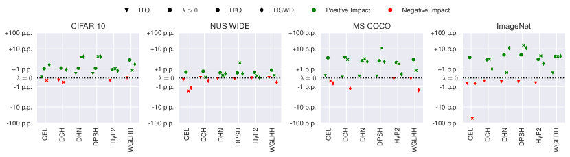
Figure 2: Variation of mAP@k in percentage points (p.p.) of each quantization strategy relative to no quantization ($\lambda=0$) on VGG-16 with $k=16$ bits. Unlike ITQ, HWSD and quantization penalty terms ($\lambda>0$), H²Q always increases the performance metric.

4.2 Improvements over Similarity-based Losses

An important consideration regarding a quantization strategy is whether it can negatively affect the performance of the learned embedding. Table 2 shows that H²Q is always able to improve each of our deep hashing benchmarks relative to the same method without quantization when using the AlexNet architecture. The average improvement is 3.6%, while the maximum improvement is 13.5%. Table A5 contains the results for the VGG-16 architecture, with the same conclusion. (Note that DPSH has the same similarity term as DHN, thus we do not report it to avoid redundancy.)

4.3 Comparison Against Other Quantization Benchmarks

On the other hand, Figure 2 shows that, for the VGG-16 network and $k=16$ bits, all the other quantization strategies considered sometimes hurt performance relative to running the same method with no penalization ($\lambda=0$). Section B.3 contains similar results for other architectures and number of bits. While H²Q systematically improves the metrics and is competitive with other methods, ITQ frequently reduces the mAP@k; when it provides improvements, they are usually smaller than those of H²Q. Using the original penalization terms ($\lambda>0$) is often more competitive than ITQ, but can also reduce the mAP@k and does not outperform H²Q consistently. HWSD performs better than ITQ, but can also reduce the mAP@k and does not outperform H²Q consistently.

4.4 Ablation Study

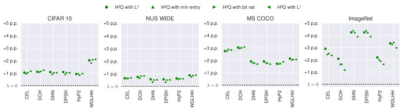
Figure 3: Increase in mAP@k in percentage points (p.p.) after using H²Q as a quantization strategy with different underlying losses, relative to no quantization ($\lambda=0$). On VGG-16 with $k=16$ bits. The increase is consistently positive and generally uniform across loss functions.

In (3.7), we proposed optimizing the $L_{2}$ distance between the rotated embedding $Uf_{\theta}(x_{i})$ and its quantization $\operatorname*{sign}(Uf_{\theta}(x_{i}))$. Still, since we are optimizing via SGD, it is easy to consider any other differentiable metric in the optimization. In this section, we study the effect of using three other reasonable loss functions beyond $L_{2}$ in (3.7). For simplicity, let $z_{i}=z_{i}(U)=Uf_{\theta}(x_{i})$ for every $i=1,\dots,n$ and $z_{i}^{j}$ be the j-th coordinate of $z_{i}$.

$\mathbf{L_{1}}:$ The alternative is to simply replace the $L_{2}$ distance by $L_{1}$. For that we change (3.7) to

$$\min_{v_{1},\dots,v_{k}\in\mathbb{R}^{k}}\frac{1}{n}\sum_{i=1}^{n}\|z_{i}-\operatorname*{sign}\left(z_{i}\right)\|_{1}.$$ (4.1)

As before, this simply measures the distance between the rotated embedding to its quantization.

min entry: Another strategy is to ensure that no coordinate of $z_{i}$ is too close to $0$. Since the LogSumExp (LSE) function is a smooth version of the maximum we can solve

$$\min_{v_{1},\dots,v_{k}\in\mathbb{R}^{k}}\frac{1}{n}\sum_{i=1}^{n}\mbox{LSE}(-(z_{i})^{2}),$$ (4.2)

where the square in $(z_{i})^{2}$ is done entry-wise.

bit var: Another alternative is to guarantee with high probability that no coordinate of $z_{i}$ is too small. Let $\xi$ be a random vector in $\mathbb{R}^{k}$ with i.i.d. entries drawn from a law with cumulative distribution function (CDF) $F$. We minimize the sum of the variance of the components of $\operatorname*{sign}(z_{i}+\xi)$:

$$\min_{v_{1},\dots,v_{k}\in\mathbb{R}^{k}}\frac{1}{n}\sum_{i=1}^{n}\sum_{j=1}^{k}F(z_{i}^{j})(1-F(z_{i}^{j})).$$ (4.3)

The goal is to ensure that $z_{i}$ is far from the regions where there might be a change of sign. In our experiments we take $F=(1+e^{-x})^{-1}$, the CDF of the logistic distribution.

The comparisons between the $L_{2}$ loss and the other three choices are shown in Figure 3. While $L_{2}$ generally outperforms other alternatives, one might still prefer them for specific datasets and similarity losses. For example, WGLHH in CIFAR 10 attains better results using (4.2) or (4.3). The fact that there is little variation across loss function performance suggests that choosing the $L_{2}$ loss is close to the best possible alternative for orthogonal transformations.

4.5 Computational Cost

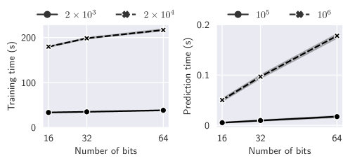
Figure 4: Training and prediction times for different number of bits. We vary the size of the training fold in $\{2\times 10^{3},2\times 10^{4}\}$ and predict $\{10^{5},10^{6}\}$ hashes, respectively. Training time is at most 3 minutes and prediction time is less than a second.

A final concern regarding H²Q is the speed at which this quantization strategy can be executed. First, note that the only trainable parameters are the vectors $v_{1},\cdots,v_{k}\in\mathbb{R}^{k}$ from (3.9), a total of $k^{2}$ parameters. Using 32-bits float representation that gives 1kB, 4kB and 16kB for 16, 32 and 64 bits, respectively, and easily fitting in the L1 cache of any modern CPU. Moreover, a training set of 20,000 embeddings fits in 5MB in the 64-bits case, which fits in L2 cache. Thus, training can be performed without the need of a GPU. Indeed, it is faster to train on CPU to reduce latency.

Figure 4 shows the computational times for training and prediction, using the $L_{2}$ loss (3.7), a batch size of 128 and 300 epochs. Times were evaluated on a i9-13900K CPU (with L1 cache of 1.4MB, L2 of 34MB) with 128GB of RAM. Even on the 64 bits case, training on a CPU with 20,000 sample points takes around 3 minutes and predicting the hashes for $10^{6}$ sample points takes only 0.2 seconds.

5 Conclusion

We propose H²Q, a novel quantization strategy for deep hashing that decomposes the learning to hash problem in two separate steps. First, perform similarity learning in the embedding space; second, optimize an orthogonal transformation to reduce quantization error. This stands in contrast to the prevalent quantization strategy, which jointly optimizes for both the embedding and the quantization error. Because H²Q relies on orthogonal transformations, it is able to minimize the quantization error while degrading the embedding by exploring an invariance in the similarity learning setup. H²Q is fast and hyperparameter-free, and uses a Householder matrix characterization of the orthogonal group along with SGD for quick computation. Unlike other popular quantization strategies, H²Q never hurts the embedding performance, and is able to significantly improve current benchmarks to deliver state-of-the-art performance in image retrieval tasks. A future avenue of work is exploring how H²Q can be combined with state-of-the-art metric learning methods on domains other than image retrieval. We hope our work encourages researchers to explore further invariances available in common loss functions to improve on learning to hash techniques and, more broadly, large-scale similarity search.

Reproducibility

The companion code for this work can be found at https://github.com/Lucas-Schwengber/h2q.

Appendices

Appendix A Setup details

We carefully reproduce the same parameters and training conditions proposed by the original paper of each similarity loss we used in our experiments. Meanwhile, we also needed to standardize our experimental setup. This section exhaustively describes the choices we made.

A.1 Architectures

We adapted two well known CNNs for the image classification problem to learning to hash. The goal of each CNN will be to learn a embedding map that maps an image into a point in $\mathbb{R}^{k}$. The hash is obtained taking the sign point-wise on the embedding. The CNNs adapted were the AlexNet and the VGG-16.

Since the original architectures are built to perform classification in ImageNet their last layer is a FC with output dimension $1000$. We replace this last layer with a new layer with output dimension $k$. We used the implementation of [7], which is available in their GitHub repository.

A.2 Optimization

A.2.1 Learning the Embeddings

We use the Adam optimizer with a learning rate of $10^{-5}$ both to train AlexNet and VGG-16. We also set a weight decay of $5\times 10^{-4}$ for all losses, except for WGLHH that uses $10^{-4}$. This is in line with the recommendation by the original papers of each loss.

The learning rate of the last layer of both adapted architectures (the hash layer), which is not pretrained, is set as $10^{-4}$. The proxies of the HyP² loss are trained with a learning rate of $10^{-3}$.

We also use the validation set to perform validation at the end of each epoch. During the validation we evaluated the mAP metric choosing from the validation set in a set of $100$ queries and a set of $900$ possible retrieval images. To mitigate the effects of randomness we took the average mAP of five random splits. We implemented an early stopping callback to halt the training if there is no observed improvement in the mAP over a span of 20 epochs. The maximum number of epochs was set to 100.

A.2.2 Learning the Orthogonal Transformations

The orthogonal transformations are all trained using the Householder parametrization with the Adam optimizer, as discussed in the main text. The learning rate used for each of the four loss functions presented are different. The $L_{2}$, $L_{1}$ and the min entry losses all use $0.1$, but the bit var loss uses $0.01$. In all cases we use a batch size of $128$ and $300$ epochs.

A.3 Deep Hashing Benchmark Losses

Let $n$ be the size of the mini-batch, $o_{1},\dots,o_{n}\in\mathbb{R}^{l}$ be the embeddings of images $x_{1},\dots,x_{n}$ and let $s_{ij}=1$ if $x_{i}$ and $x_{j}$ are similar and $s_{ij}=0$ otherwise. The cosine-similarity between $o_{i}$ and $o_{j}$ will be denoted by

$$c_{ij}=\frac{\langle o_{i},o_{j}\rangle}{\|o_{i}\|_{2}\|o_{j}\|_{2}},$$

and the generalized hamming distance by

$$d_{ij}=\frac{k}{2}(1-c_{ij}).$$

Another important quantity is $w_{ij}$. This quantity aims to correct the unbalance between the amount of similar and dissimilar pairs. We define:

$$w_{ij}=\frac{s_{ij}}{p}+\frac{1-s_{ij}}{1-p}.$$

where $p$ is the percentage of similar pairs in the training set.

Let $C$ be the number of classes of a dataset and $y_{i}\in\{0,1\}^{C}$ be the one hot labels of $x_{i}$. On CIFAR 10 and ImageNet each $x_{i}$ belong to one and only one class, while in NUS WIDE and MS COCO each $x_{i}$ can be in more than one class at the same time. In both cases the similarity between $i$ and $j$ is given by:

$$s_{ij}=\textbf{1}_{[\langle y_{i},y_{j}\rangle>0]}.$$

We now specialize the expression of the loss function of each benchmark following (3.3).

A.3.1 Cosine Embedding Loss (CEL) [4]

For this loss,

$$L_{S}=\frac{1}{n^{2}}\sum_{i,j}s_{ij}\left(1-c_{ij}\right)+(1-s_{ij})\left(c_{ij}-\delta\right)_{+}$$

and

$$L_{Q}=\frac{1}{n}\sum_{i=1}^{n}\|o_{i}-h_{i}\|_{2}^{2}.$$

The original CEL does not have a penalty term since it is used for metric learning. We add a penalty term to provide comparisons with such type of quantization strategy (i.e., $\lambda>0$). The main parameter is the margin $\delta$ and is taken from [5], the batch size is 128. The penalty used was $\lambda=0.01$.

A.3.2 Deep Cauchy Hashing (DCH) [6]

For this loss,

$$L_{S}=\frac{1}{n^{2}}\sum_{i,j}w_{ij}\left(s_{ij}\log\frac{d_{ij}}{\gamma}+\log\frac{1+\gamma}{d_{ij}}\right)$$

and

$$L_{Q}=\frac{1}{n}\sum_{i=1}^{n}\log\left(1+\gamma^{-1}\frac{k}{2}\left(1-\frac{\langle o_{i},h_{i}\rangle}{\|o_{i}\|_{2}\|h_{i}\|_{2}}\right)\right).$$

We let $\gamma=10$ and a batch size of 256, as recommended in their paper (see Figure 5 of [6]). The penalty $\lambda$ was selected between the values $10^{-5}$, $10^{-3}$, and $10^{-1}$ using the validation set.

A.3.3 Deep Hashing Network (DHN) [63]

For this loss,

$$L_{S}=\frac{1}{n^{2}}\sum_{i,j}s_{ij}\langle o_{i},o_{j}\rangle+\log\frac{1}{1+e^{-\langle o_{i},o_{j}\rangle}}$$

and

$$L_{Q}=\frac{1}{n}\sum_{i=1}^{n}\sum_{l=1}^{k}\log\frac{\cosh|o_{il}|}{e}.$$

We let a batch size of 64, as recommended in their paper. The penalty $\lambda$ was selected between the values $10^{-5}$, $10^{-3}$, and $10^{-1}$ using the validation set.

A.3.4 Deep Pairwise-Supervised Hashing (DPSH) [36]

DPSH has the same similarity loss as DHN,

$$L_{S}=\frac{1}{n^{2}}\sum_{i,j}s_{ij}\langle o_{i},o_{j}\rangle+\log\frac{1}{1+e^{-\langle o_{i},o_{j}\rangle}},$$

but the quantization loss is different:

$$L_{Q}=\frac{1}{n}\sum_{i=1}^{n}\|o_{i}-h_{i}\|_{2}^{2}.$$

We let a batch size of 128. The penalty $\lambda$ was selected between the values $10^{-2}$, $10^{-1}$, and $1$ using the validation set.

A.3.5 Weighted Gaussian Loss Hamming Hashing (WGLHH) [51]

For this loss,

$$L_{S}= \frac{1}{n^{2}}\sum_{i,j}a_{ij}w_{ij}s_{ij}\log\frac{2s_{ij}}{s_{ij}+\exp(-\alpha d_{ij}^{2})}+\frac{1}{n^{2}}\sum_{i,j}a_{ij}w_{ij}\exp(-\alpha d_{ij}^{2})\log\frac{2\exp(-\alpha d_{ij}^{2})}{s_{ij}+\exp(-\alpha d_{ij}^{2})}.$$

with

$$a_{ij}=\exp\left(\frac{s_{ij}-c_{ij}}{2}\right).$$

The quantization loss is

$$L_{Q}=\frac{1}{n}\sum_{i=1}^{n}\|o_{i}-h_{i}\|_{2}^{2}.$$

We let $\alpha=0.1$, a batch size of 64 and $\lambda=0.001$, as recommended in the original paper.

A.3.6 HyP² [59]

For this loss we start defining a first term that is based on the dissimilar pairs:

$$L_{D}=\frac{\sum_{i,j}(1-s_{ij})(c_{ij}-\delta)_{+}}{\sum_{i,j}(1-s_{ij})}.$$

In this case a list of $C$ proxies are also trained. Each proxy stands for a class $1,\dots,C$ and tries to capture the “average embedding” of a class. Let $p_{1},\dots,p_{C}\in\mathbb{R}^{k}$ be the proxies. Define

$$L_{P}= -\frac{\sum_{i=1}^{n}\sum_{l=1}^{C}y_{il}\frac{\langle o_{i},p_{l}\rangle}{\|o_{i}\|\|p_{l}\|}}{\sum_{i=1}^{n}\sum_{l=1}^{C}y_{il}}+\frac{\sum_{i=1}^{n}\sum_{l=1}^{C}(1-y_{il})\left(\frac{\langle o_{i},p_{l}\rangle}{\|o_{i}\|\|p_{l}\|}-\delta\right)_{+}}{\sum_{i=1}^{n}\sum_{l=1}^{C}(1-y_{il})}$$

Finally,

$$L_{S}=L_{P}+\beta L_{D}$$

and

$$L_{Q}=\frac{1}{n}\sum_{i=1}^{n}\|o_{i}-h_{i}\|_{2}^{2}.$$

The quantization loss $L_{Q}$ is not originally proposed in their paper since their paper uses no quantization. We add the $L_{Q}$ loss in our experiments only for the case $\lambda>0$. For benchmarks we consider their original formulation. The parameter $\delta$ is taken from [5]. We followed the recommended batch size of 100. $\beta$ was selected among the values in $[0.5,0.75,1.0,1.25]$, the choice was performed on the validation set to maximize mAP@k. Since the method does not use a quantization penalty term $L_{Q}$, we set $\lambda=0.01$, as it is close to the default value for other methods.

A.3.7 HashNet [7]

HashNet takes another approach to quantization: instead of adding a penalty, they take $\beta\to\infty$ and evaluate their loss in $\tanh(\beta o_{i})$, thus making the quantization error

$$\|\tanh(\beta o_{i})-h_{i}\|_{2}$$

small. This quantization strategy is quite interesting, but is out of the scope of our work. We use HashNet as a hashing benchmark, but we do not experiment with it adding penalties or rotations. Our implementation directly follows the code available in their GitHub repository, the main parameter is $\beta$, which we take as

$$\left(1+\frac{b}{200}\right)^{\frac{1}{2}},$$

where $b$ is the number of batches iterated until a moment (this number accumulates every epoch). The batch size used was $256$.

A.3.8 ADSH [24]

ADSH learns the hash functions in two separate ways. For the points on the database, the hash codes are learned directly, while for out-of-sample extensions the hash codes come from binarizing the output of a neural network. The full optimization problem is formulated as:

$$\begin{split}\min_{V,\Theta}\sum_{i=1}^{m}\sum_{j=1}^{n}\left[\tanh\left(F\left(\textbf{x}_{i},\Theta\right)\right)^{\intercal}\textbf{v}_{j}-cS_{ij}\right]^{2},\\ \text{s.t. }V\in\{-1,+1\}^{n\times k},\end{split}$$ (A.1)

where $n$ is the size of the database and $m$ is the size of a random subset of images from the database. Their learning algorithm iterate between doing gradient descent updates on $\Theta$ using the random subset of the database and then updating the hash codes $V$ for the database points directly using a formula from linear algebra. Since they use the whole database for training, to make fair comparisons with the other methods, which are trained on the training set, we restrict the training step to the training set. The binary representation of each image is obtained using the out-of-sample extension provided by the neural network architecture.

As for the choice of hyper parameters, as in the original paper, we take the maximum number of iterations to be $T_{\text{out}}=50$, the strength of the penalization to be $\gamma=200$, and the number of epochs per iteration to be $T_{\text{in}}=3$. Differently from the original paper, we took the sample size to be $|\Omega|=5000$ and the mini-batch size to be $64$ as this seemed to give better results in our setting. We set the starting learning rate to $10^{-5}$.

A.4 Quantization Benchmarks

In our work we study four main quantization strategies:

• The baseline is to use no quantization strategy, here we train using the the benchmark losses described in Section A.3 with the quantization penalty set to zero;

• The second is to use the original quantization strategy proposed by each deep hashing method, that is to train using some penalty $\lambda>0$;

• We also test our proposed quantization strategy, which consists of learning a rotation on top of the baseline;

• We also use the Iterative Quantization strategy [19], which also tries to learn a rotation on top of the baseline, but using an iterative and less-efficient process;

• Finally, we also add the HSWD quantization strategy proposed in [20] as a benchmark. This strategy simply replaces the original quantization loss term by another fixed quantization loss and train the embedding with the added penalty.

We now describe some implementation details of the previously listed quantization strategies.

A.5 Baseline and Original Quantization Strategies

For the baseline we use no $\tanh$ activation layer and set $\lambda=0$. All other parameters are as described in Section A.3. For the original quantization strategies we use the $\tanh$ activation layer. The penalty parameter $\lambda$ and all the other are as described in Section A.3.

A.5.1 ITQ

Our implementation of ITQ follows this GitHub repository. The ITQ is originally design to obtain the embeddings using PCA decomposition. To adapt the method to be a quantization strategy for deep hashing methods we use the embeddings learned by the baseline as input. The main parameter is the number of iterations, we take it to be $50$. We also experiment if centralizing the embeddings (as is usually done when PCA is performed) would increase the performance, but it was not the case.

A.5.2 HSWD

This method simply exchange the original quantization term $L_{Q}$ of the deep hashing methods by another quantization term. We adapted the original implementation from their GitHub repository. The main parameter is the quantization penalty used, we follow the recommendation presented in their code and use $\lambda=0.1$, we also do not use the $\tanh$ activation. All the other parameters follows the default parameter listed in Section A.3.

Appendix B Experimental Results

	CIFAR 10				NUS WIDE				MS COCO				ImageNet
n bits	16	32	48	64	16	32	48	64	16	32	48	64	16	32	48	64
ADSH	56.7	71.8	77.3	79.7	74.8	78.4	79.8	80.3	57.9	61.1	63.7	65.0	5.2	8.3	13.4	23.2
CEL	79.8	81.0	81.7	81.3	79.4	80.3	80.7	80.7	64.4	66.3	67.5	68.4	51.8	52.5	53.7	45.6
DHN	81.2	81.1	81.1	81.3	80.6	81.3	81.6	81.7	66.8	67.3	69.2	69.4	25.1	32.4	35.7	38.2
DCH	80.2	80.1	80.0	79.8	78.4	79.1	79.1	79.8	63.8	66.2	67.1	66.7	58.2	58.8	58.9	60.4
DPSH	81.2	81.2	81.5	81.1	81.0	81.9	82.1	82.1	68.0	71.2	71.6	72.4	36.5	42.2	46.0	49.9
HashNet	80.8	82.1	82.3	82.3	79.8	81.5	82.2	82.7	62.9	67.3	68.2	70.2	41.2	54.3	58.8	62.5
WGLHH	79.6	80.0	80.2	79.4	79.9	80.7	80.1	80.5	66.3	67.0	67.7	67.2	55.3	57.1	57.0	56.8
HyP²	80.5	81.1	81.7	81.8	81.9	82.5	83.1	83.0	71.9	74.1	74.8	74.9	54.1	56.9	57.7	56.5
HyP² + ITQ	80.2	80.7	81.4	81.8	81.6	82.5	83.0	83.0	71.6	73.9	74.8	74.8	53.5	56.7	57.6	56.3
HyP² + HSWD	82.1	82.3	82.4	82.0	82.0	82.6	83.2	83.1	72.1	74.7	74.9	74.9	56.8	60.2	60.8	58.8
HyP² + H²Q	82.3	82.5	82.9	83.1	82.5	83.2	83.4	83.3	73.9	75.4	75.9	75.7	57.3	60.7	61.5	60.6

Table A3: mAP@k with AlexNet. We compare the best performance metrics of each benchmark with HyP² combined with H²Q.

	CIFAR 10				NUS WIDE				MS COCO				ImageNet
n bits	16	32	48	64	16	32	48	64	16	32	48	64	16	32	48	64
ADSH	64.4	80.3	84.1	85.0	79.1	82.3	83.2	83.5	62.2	65.6	67.5	69.2	10.8	22.7	39.7	56.2
CEL	85.1	85.6	85.8	85.7	82.7	83.1	83.3	82.8	73.3	75.7	76.2	76.4	69.9	72.8	74.4	72.5
DCH	84.0	82.9	82.8	82.9	81.9	81.8	81.1	81.2	75.7	76.0	76.7	76.0	79.8	80.2	79.8	80.1
DHN	86.2	86.6	86.9	86.6	83.2	83.6	83.6	83.7	68.6	70.7	69.9	71.5	45.4	54.4	59.1	62.3
DPSH	86.4	86.8	86.5	86.7	84.5	85.0	85.2	85.5	77.4	79.0	79.7	79.1	61.6	68.8	71.6	74.0
HashNet	85.7	86.1	86.4	86.2	83.2	84.1	84.6	85.0	68.3	72.2	74.3	75.5	65.0	74.7	79.2	80.8
WGLHH	84.5	83.6	84.2	83.3	83.8	83.6	83.4	83.0	78.1	75.9	76.9	76.6	79.6	79.4	79.0	78.2
HyP²	85.0	85.2	85.6	85.7	85.1	85.5	85.9	85.9	79.7	82.0	82.6	82.2	75.7	77.5	79.0	78.8
HyP² + ITQ	84.7	85.0	85.6	85.5	85.1	85.6	85.8	85.9	79.6	81.9	82.6	82.1	75.1	77.0	78.4	78.8
HyP² + HSWD	85.8	85.6	85.8	86.0	85.1	85.4	85.7	85.7	80.1	81.8	82.2	81.6	77.3	79.3	80.0	78.8
HyP² + H²Q	86.0	86.3	86.4	86.4	85.7	86.0	86.1	86.1	81.4	82.7	83.1	82.4	77.9	80.6	81.5	81.5

Table A4: mAP@k with VGG-16. We compare the best performance metrics of each benchmark with HyP² combined with H²Q.

	CIFAR 10				NUS WIDE				MS COCO				ImageNet
n bits	16	32	48	64	16	32	48	64	16	32	48	64	16	32	48	64
CEL ($\lambda=0$)	85.1	85.6	85.8	85.7	82.7	83.1	83.3	82.8	73.3	75.7	76.2	76.4	69.9	72.8	74.4	72.5
CEL + H²Q	86.1	86.5	86.8	86.6	83.4	84.0	84.3	84.1	76.1	78.0	78.5	78.5	72.8	75.8	77.3	75.8
DHN ($\lambda=0$)	83.1	85.5	85.9	85.8	82.9	83.2	83.6	83.3	66.3	69.5	70.0	71.4	44.8	55.6	59.9	62.5
DHN + H²Q	84.2	86.2	86.8	86.8	83.4	83.9	84.1	83.9	68.2	71.7	72.7	73.7	49.1	59.9	64.1	66.1
DCH ($\lambda=0$)	84.5	82.6	80.1	80.2	81.9	81.3	80.5	80.0	73.5	69.4	70.0	68.4	77.5	75.6	72.2	69.6
DCH + H²Q	85.6	83.9	81.9	81.8	82.6	82.3	81.5	80.9	76.5	72.6	72.9	71.3	79.6	78.0	74.7	72.4
WGLHH ($\lambda=0$)	83.6	81.9	80.9	80.6	83.5	82.9	82.6	82.4	77.2	73.8	74.9	75.5	76.2	75.1	75.4	77.0
WGLHH + H²Q	85.6	84.3	83.1	83.3	84.4	83.9	83.4	83.4	79.4	76.0	77.1	77.6	79.6	78.5	78.4	79.2
HyP² ($\lambda=0$)	85.0	85.2	85.6	85.7	85.1	85.5	85.9	85.9	79.7	82.0	82.6	82.2	75.7	77.5	79.0	78.8
HyP² + H²Q	86.0	86.3	86.4	86.4	85.7	86.0	86.1	86.1	81.4	82.7	83.1	82.4	77.9	80.6	81.5	81.5

Table A5: mAP@k with VGG-16. We show the effect of using H²Q on each method after training with no $tanh$ activation and no quantization term ($\lambda=0$).

B.1 Improvements over Existing Benchmarks

Table A3 is an extended version of Table 1 of the main text, and Table A4 is its analogous to the VGG-16 architecture. The HyP²  with our quantization strategy is the winning strategy in the majority of the cases also for the VGG-16.

B.2 Improvements over Similarity-based Losses

Here we extend the discussion provided in Section 4.2 of the main text. Table A5 is the analogous of Table 2 of the main text, but for the VGG-16 architecture. As observed for the AlexNet, we uniformly improved the performance of similarity-based losses also for the VGG-16 architecture. We have an average improvement of $2.6\%$ and a maximum of $9.5\%$.

	CIFAR 10				NUS WIDE				MS COCO				ImageNet
n bits	16	32	48	64	16	32	48	64	16	32	48	64	16	32	48	64
CEL($\lambda=0$)	79.80.6	81.00.4	81.70.3	81.30.2	79.40.2	80.30.2	80.70.2	80.70.3	64.40.5	66.30.6	67.50.3	68.40.4	51.81.1	52.50.3	53.71.1	45.60.5
CEL+ITQ	79.80.5	80.60.4	81.50.1	81.30.3	79.40.1	80.50.3	80.40.2	80.70.4	64.40.3	66.40.4	67.80.3	68.70.2	51.70.9	53.00.5	53.70.8	45.70.5
CEL+$\lambda$	80.20.3	79.11.0	77.80.4	70.72.7	79.20.2	79.80.3	79.60.1	79.00.4	66.10.3	67.10.2	67.30.5	66.90.2	19.10.8	22.20.9	23.30.1	25.50.5
CEL+HSWD	82.00.6	82.40.6	82.80.5	82.90.6	79.90.3	80.60.5	81.00.4	81.10.4	64.30.6	66.30.6	67.60.8	68.30.5	43.80.1	48.10.3	49.50.2	46.90.5
CEL+H²Q($L_{2}$)	82.20.5	82.40.1	82.70.1	82.40.2	80.60.2	81.90.2	82.20.1	82.30.3	66.40.4	68.50.3	69.60.2	70.20.2	54.60.7	55.00.4	56.10.7	48.40.7
CEL+H²Q($L_{1}$)	82.30.6	82.50.2	82.70.2	82.50.3	80.60.2	81.80.2	82.10.1	82.30.3	66.50.4	68.40.3	69.60.2	70.20.2	54.30.7	54.80.5	55.90.6	48.60.7
CEL+H²Q(min)	82.40.4	82.40.2	82.70.2	82.50.4	80.70.2	81.80.3	82.20.1	82.30.3	66.40.3	68.50.4	69.70.2	70.40.2	54.20.7	54.60.7	56.00.7	48.50.5
CEL+H²Q(bit)	82.30.4	82.30.2	82.70.3	82.50.3	80.70.2	81.80.2	82.20.1	82.30.3	66.40.3	68.50.3	69.60.2	70.30.2	53.70.8	54.60.6	55.60.7	48.30.7
DCH($\lambda=0$)	78.30.5	77.51.1	77.30.4	76.31.1	78.80.5	78.90.4	78.50.2	78.60.2	62.81.1	64.10.4	64.20.2	64.30.2	50.92.1	49.61.2	48.51.2	46.51.1
DCH+ITQ	78.40.5	77.10.9	77.20.4	76.51.0	78.50.4	78.80.4	78.20.3	78.70.3	62.50.8	63.80.4	64.50.2	64.60.2	51.21.5	49.60.9	48.21.3	46.91.5
DCH+$\lambda$	80.20.5	80.10.4	80.00.4	79.80.4	78.40.2	79.10.2	79.10.2	79.80.3	63.81.1	66.20.6	67.11.6	66.70.7	58.20.9	58.80.7	58.91.5	60.40.7
DCH+HSWD	81.00.9	80.00.5	79.30.1	78.12.3	79.20.4	78.90.2	78.30.1	78.20.2	62.80.7	63.71.0	64.30.5	63.90.6	56.50.9	52.01.3	50.51.7	48.31.2
DCH+H²Q($L_{2}$)	81.60.5	80.30.6	80.10.3	79.40.6	79.60.4	79.90.2	79.70.1	80.10.3	64.31.3	66.00.2	66.10.1	66.10.1	55.01.3	53.51.0	51.91.1	50.00.7
DCH+H²Q($L_{1}$)	81.60.1	80.30.6	80.10.3	79.20.8	79.70.4	79.90.2	79.60.2	80.00.3	64.51.1	66.00.2	66.10.1	66.20.2	55.01.5	53.01.1	51.30.9	49.21.0
DCH+H²Q(min)	81.70.3	80.40.6	80.00.1	79.10.5	79.70.3	80.00.2	79.70.1	80.10.3	64.71.2	66.00.1	66.10.1	66.20.2	54.81.3	52.60.9	51.01.2	48.50.6
DCH+H²Q(bit)	81.70.3	80.20.4	79.60.3	78.90.6	79.70.4	80.00.2	79.70.1	80.20.4	64.61.1	65.90.2	66.10.1	66.10.2	54.71.3	52.61.0	50.30.9	48.00.9
DHN($\lambda=0$)	78.91.1	79.50.5	78.70.6	79.40.4	79.60.2	80.40.3	80.90.3	81.30.2	62.91.5	65.51.4	66.53.1	67.42.5	24.10.6	31.80.5	34.20.7	36.71.3
DHN+ITQ	79.11.0	79.20.6	78.71.0	79.30.4	79.60.1	80.40.1	81.00.2	81.50.2	63.11.1	65.51.5	66.63.2	67.82.7	24.21.1	31.80.4	34.20.9	36.51.3
DHN+$\lambda$	81.20.3	81.10.6	81.10.3	81.30.3	80.60.4	81.30.2	81.60.2	81.70.2	66.81.4	67.31.0	69.21.4	69.41.1	25.10.6	32.40.4	35.71.2	38.20.3
DHN+HSWD	81.20.7	81.40.5	81.00.7	80.40.4	80.70.1	81.40.3	81.90.2	81.80.0	63.81.0	67.91.7	67.31.5	68.91.2	33.10.7	39.90.6	42.80.3	44.40.5
DHN+H²Q($L_{2}$)	80.50.5	80.70.6	79.90.7	80.50.6	80.50.3	81.40.2	81.50.2	82.00.2	64.61.4	67.21.4	68.03.1	68.92.7	26.01.3	34.40.4	36.41.1	38.81.5
DHN+H²Q($L_{1}$)	80.60.5	80.70.5	80.10.7	80.50.5	80.30.4	81.20.2	81.40.2	81.80.1	64.21.4	66.91.5	67.83.0	68.82.7	25.81.2	34.30.3	36.41.1	38.81.7
DHN+H²Q(min)	80.60.8	80.80.4	80.00.8	80.40.5	80.50.3	81.40.2	81.50.2	81.90.3	64.51.4	67.21.5	68.13.1	69.02.7	25.91.3	34.40.2	36.41.0	38.91.7
DHN+H²Q(bit)	80.70.6	80.80.4	80.10.8	80.50.4	80.50.3	81.40.1	81.70.2	82.00.1	64.41.4	67.11.6	68.13.2	69.02.7	25.61.1	34.30.4	36.20.8	38.51.7
DPSH($\lambda=0$)	78.91.1	79.50.5	78.70.6	79.40.4	79.60.2	80.40.3	80.90.3	81.30.2	62.91.5	65.51.4	66.53.1	67.42.5	24.10.6	31.80.5	34.20.7	36.71.3
DPSH+ITQ	79.11.0	79.20.6	78.71.0	79.30.4	79.60.1	80.40.1	81.00.2	81.50.2	63.11.1	65.51.5	66.63.2	67.82.7	24.21.1	31.80.4	34.20.9	36.51.3
DPSH+$\lambda$	81.20.7	81.20.2	81.50.5	81.10.4	81.00.3	81.90.1	82.10.3	82.10.4	68.01.6	71.20.1	71.61.3	72.40.2	36.51.7	42.21.7	46.01.0	49.90.3
DPSH+HSWD	81.20.7	81.40.5	81.00.7	80.40.4	80.70.1	81.40.3	81.90.2	81.80.0	63.81.0	67.91.7	67.31.5	68.91.2	33.10.7	39.90.6	42.80.3	44.40.5
DPSH+H²Q($L_{2}$)	80.50.5	80.70.6	79.90.7	80.50.6	80.50.3	81.40.2	81.50.2	82.00.2	64.61.4	67.21.4	68.03.1	68.92.7	26.01.3	34.40.4	36.41.1	38.81.5
DPSH+H²Q($L_{1}$)	80.60.5	80.70.5	80.10.7	80.50.5	80.30.4	81.20.2	81.40.2	81.80.1	64.21.4	66.91.5	67.83.0	68.82.7	25.81.2	34.30.3	36.41.1	38.81.7
DPSH+H²Q(min)	80.60.8	80.80.4	80.00.8	80.40.5	80.50.3	81.40.2	81.50.2	81.90.3	64.51.4	67.21.5	68.13.1	69.02.7	25.91.3	34.40.2	36.41.0	38.91.7
DPSH+H²Q(bit)	80.70.6	80.80.4	80.10.8	80.50.4	80.50.3	81.40.1	81.70.2	82.00.1	64.41.4	67.11.6	68.13.2	69.02.7	25.61.1	34.30.4	36.20.8	38.51.7
WGL.($\lambda=0$)	78.30.5	76.90.5	75.60.7	76.10.5	79.40.6	79.60.4	79.40.5	78.80.3	64.41.2	64.00.4	64.00.2	64.00.3	49.81.9	46.50.6	47.62.2	48.41.8
WGL.+ITQ	77.91.0	77.60.6	76.11.1	76.21.2	79.30.4	79.70.5	79.40.6	79.10.4	63.90.7	64.10.3	64.10.2	64.70.3	49.51.7	47.40.9	48.12.5	49.21.8
WGL.+$\lambda$	79.60.8	80.00.2	80.20.2	79.41.7	79.90.2	80.70.5	80.10.4	80.50.7	66.31.9	67.01.4	67.71.4	67.21.4	55.31.3	57.11.1	57.00.9	56.80.7
WGL.+HSWD	79.00.5	79.20.8	77.70.6	76.40.8	79.70.3	79.00.2	78.30.8	78.50.2	65.12.2	67.20.7	65.62.1	65.60.3	55.31.4	52.00.9	47.41.3	47.22.1
WGL.+H²Q($L_{2}$)	81.60.3	80.90.6	80.50.2	80.20.2	81.00.3	81.70.3	81.20.2	81.40.2	66.20.9	66.50.4	66.80.3	66.70.2	54.41.5	52.80.8	53.91.9	54.71.4
WGL.+H²Q($L_{1}$)	81.90.3	81.10.6	80.60.3	80.30.6	81.10.3	81.60.2	81.30.2	81.20.3	66.10.8	66.40.5	66.80.3	66.60.3	54.51.5	52.50.4	53.62.1	53.91.5
WGL.+H²Q(min)	82.00.7	81.00.6	81.00.4	80.70.2	80.90.3	81.70.2	81.40.1	81.30.3	66.20.7	66.50.4	66.80.3	66.70.2	54.11.1	52.70.7	53.71.5	54.11.8
WGL.+H²Q(bit)	81.90.5	81.10.5	81.00.3	80.70.4	81.00.4	81.70.3	81.30.3	81.40.3	66.21.0	66.30.3	66.60.3	66.50.3	53.81.6	52.00.8	53.21.8	53.91.2
HyP²($\lambda=0$)	80.50.8	81.10.5	81.70.3	81.80.5	81.90.1	82.50.2	83.10.1	83.00.2	71.90.4	74.10.4	74.80.2	74.90.6	54.11.4	56.90.4	57.70.5	56.50.2
HyP²+ITQ	80.20.2	80.70.7	81.40.2	81.80.5	81.60.3	82.50.2	83.00.1	83.00.2	71.60.7	73.90.2	74.80.2	74.80.6	53.51.5	56.70.5	57.60.4	56.30.5
HyP²+$\lambda$	82.10.3	82.20.1	82.20.3	82.10.3	82.10.1	82.50.2	82.70.2	82.50.2	73.00.4	73.60.4	72.60.6	71.40.6	58.40.6	62.20.7	62.40.2	61.30.8
HyP²+HSWD	82.10.6	82.30.2	82.40.1	82.00.4	82.00.1	82.60.2	83.20.1	83.10.1	72.10.4	74.70.4	74.90.2	74.90.2	56.80.9	60.20.5	60.80.5	58.80.7
HyP²+H²Q($L_{2}$)	82.30.3	82.50.5	82.90.2	83.10.3	82.50.2	83.20.1	83.40.1	83.30.1	73.90.2	75.40.2	75.90.3	75.70.3	57.30.9	60.70.4	61.50.3	60.60.4
HyP²+H²Q($L_{1}$)	82.30.2	82.60.5	83.00.3	83.10.4	82.50.2	83.10.1	83.30.1	83.30.1	73.80.3	75.30.2	75.80.3	75.60.4	57.00.8	60.50.4	61.20.2	60.70.4
HyP²+H²Q(min)	82.30.2	82.70.5	82.80.2	83.10.3	82.60.2	83.20.2	83.40.1	83.30.2	73.90.3	75.30.2	75.90.2	75.70.3	57.10.9	60.30.3	61.30.4	60.60.3
HyP²+H²Q(bit)	82.30.2	82.70.4	82.90.2	83.00.4	82.50.2	83.20.1	83.40.1	83.30.2	73.70.2	75.30.2	75.90.3	75.60.3	56.80.8	60.00.4	60.90.1	60.20.3

Table A6: Full comparison of mAP@k before (level $\lambda=0$) and after using each quantization strategy on AlexNet. Performance metrics in red indicate a decrease in performance after the quantization strategy and performance metrics in bold indicate which quantization strategy gave the best overall metric. The small superscript numbers indicate the standard deviation of the metrics.

	CIFAR 10				NUS WIDE				MS COCO				ImageNet
n bits	16	32	48	64	16	32	48	64	16	32	48	64	16	32	48	64
CEL($\lambda=0$)	85.10.3	85.60.4	85.80.3	85.70.4	82.70.3	83.10.5	83.30.2	82.80.4	73.30.7	75.70.7	76.20.4	76.40.2	69.90.7	72.80.3	74.40.4	72.50.3
CEL+ITQ	85.20.3	85.70.1	85.50.2	85.60.4	82.50.4	83.20.3	83.30.1	83.00.5	73.50.4	75.70.9	76.30.5	76.40.5	69.30.5	73.00.3	74.20.7	72.70.1
CEL+$\lambda$	84.80.7	85.30.2	82.91.2	64.615.5	81.20.3	81.50.1	81.30.2	81.20.1	73.00.8	73.30.7	73.00.4	72.50.3	19.11.8	21.73.0	25.52.3	29.32.7
CEL+HSWD	86.60.3	86.70.3	86.90.2	87.10.3	81.60.5	82.40.2	82.40.8	82.50.6	72.70.3	75.71.0	76.00.4	75.70.9	69.30.9	72.80.9	73.61.1	71.80.2
CEL+H²Q($L_{2}$)	86.10.1	86.50.4	86.80.1	86.60.5	83.40.2	84.00.3	84.30.1	84.10.2	76.10.3	78.00.5	78.50.4	78.50.4	72.80.8	75.80.2	77.30.5	75.80.4
CEL+H²Q($L_{1}$)	86.10.2	86.60.3	86.80.2	86.50.4	83.40.2	84.00.3	84.30.1	84.00.2	76.10.4	78.00.6	78.50.5	78.50.4	72.41.0	75.70.3	77.10.6	75.80.3
CEL+H²Q(min)	86.10.1	86.60.2	86.80.1	86.60.3	83.30.3	84.10.3	84.30.1	84.10.2	76.20.4	78.00.7	78.50.5	78.50.4	72.41.0	75.50.4	77.00.4	75.50.3
CEL+H²Q(bit)	86.30.2	86.50.2	86.80.1	86.70.3	83.40.3	84.10.3	84.30.1	84.10.2	76.20.4	78.10.6	78.50.5	78.50.4	72.31.1	75.40.3	77.10.4	75.40.4
DCH($\lambda=0$)	84.50.4	82.61.2	80.11.0	80.20.2	81.90.6	81.30.1	80.50.2	80.00.3	73.50.8	69.41.7	70.01.6	68.40.7	77.50.3	75.61.2	72.21.1	69.61.2
DCH+ITQ	84.20.3	82.51.0	80.10.8	80.20.6	81.90.6	81.40.1	80.60.4	80.20.2	73.60.5	70.01.4	70.81.4	69.40.4	77.10.4	75.50.8	72.61.3	70.30.7
DCH+$\lambda$	84.00.6	82.90.6	82.80.9	82.90.2	81.90.2	81.80.4	81.10.2	81.20.2	75.70.8	76.01.2	76.71.2	76.01.2	79.80.3	80.20.5	79.80.3	80.10.5
DCH+HSWD	85.40.5	83.20.6	81.91.7	81.31.2	81.50.2	80.50.2	79.70.2	79.10.1	72.31.3	69.73.5	69.11.3	67.00.7	78.50.6	75.21.0	71.61.6	71.31.4
DCH+H²Q($L_{2}$)	85.60.2	83.90.8	81.90.5	81.80.5	82.60.3	82.30.1	81.50.2	80.90.3	76.50.6	72.61.7	72.91.3	71.30.4	79.60.6	78.00.7	74.70.8	72.40.8
DCH+H²Q($L_{1}$)	85.60.2	84.00.7	81.80.8	81.50.5	82.50.5	82.20.2	81.50.1	80.80.3	76.50.6	72.61.6	72.81.4	71.30.3	79.20.8	77.40.5	74.00.8	71.50.4
DCH+H²Q(min)	85.60.3	84.00.8	81.80.6	81.80.6	82.70.4	82.30.2	81.50.1	80.90.4	76.50.5	72.71.7	72.91.3	71.30.4	79.10.6	77.00.7	73.30.6	70.70.5
DCH+H²Q(bit)	85.70.2	84.10.8	81.80.6	81.50.5	82.70.4	82.40.1	81.60.1	80.90.3	76.60.6	72.61.7	72.91.3	71.20.5	78.70.8	76.60.8	72.80.8	70.00.3
DHN($\lambda=0$)	83.12.3	85.50.5	85.90.5	85.80.3	82.90.2	83.20.3	83.60.1	83.30.3	66.31.3	69.51.4	70.01.0	71.41.1	44.80.6	55.60.8	59.91.0	62.50.8
DHN+ITQ	83.62.1	85.50.5	85.90.5	85.90.4	82.80.3	83.20.3	83.60.1	83.30.3	66.41.3	69.81.3	70.61.1	71.71.0	44.40.6	55.10.5	59.90.8	62.50.5
DHN+$\lambda$	86.20.4	86.60.2	86.90.6	86.60.3	83.20.3	83.60.2	83.60.2	83.70.1	68.62.5	70.71.2	69.90.7	71.51.4	45.40.4	54.41.1	59.10.9	62.31.2
DHN+HSWD	86.30.5	86.90.3	86.90.2	86.50.4	83.30.1	83.70.2	83.90.3	84.10.3	68.12.0	70.31.5	70.51.0	72.81.4	56.00.7	63.90.9	66.50.7	68.10.8
DHN+H²Q($L_{2}$)	84.21.8	86.20.4	86.80.6	86.80.4	83.40.2	83.90.2	84.10.1	83.90.2	68.21.5	71.71.2	72.71.1	73.70.9	49.11.4	59.90.2	64.11.0	66.10.5
DHN+H²Q($L_{1}$)	84.02.0	86.20.4	86.80.6	86.70.5	83.20.4	83.80.2	84.00.1	83.70.2	68.11.5	71.71.4	72.61.0	73.60.8	49.21.3	59.60.2	63.91.1	65.80.6
DHN+H²Q(min)	84.11.8	86.20.3	86.80.6	86.70.4	83.40.2	83.80.2	84.00.1	83.80.3	68.01.4	72.01.3	72.61.1	73.70.9	49.01.1	59.10.6	63.71.1	66.10.7
DHN+H²Q(bit)	84.11.9	86.30.3	86.80.5	86.80.5	83.40.2	83.90.2	84.10.1	83.80.3	68.01.6	71.81.2	72.41.1	73.60.9	48.70.7	59.20.7	63.81.0	66.00.6
DPSH($\lambda=0$)	83.12.3	85.50.5	85.90.5	85.80.3	82.90.2	83.20.3	83.60.1	83.30.3	66.31.3	69.51.4	70.01.0	71.41.1	44.80.6	55.60.8	59.91.0	62.50.8
DPSH+ITQ	83.62.1	85.50.5	85.90.5	85.90.4	82.80.3	83.20.3	83.60.1	83.30.3	66.41.3	69.81.3	70.61.1	71.71.0	44.40.6	55.10.5	59.90.8	62.50.5
DPSH+$\lambda$	86.40.3	86.80.2	86.50.2	86.70.4	84.50.4	85.00.1	85.20.2	85.50.2	77.41.4	79.00.8	79.70.9	79.10.8	61.60.5	68.80.5	71.60.5	74.00.7
DPSH+HSWD	86.30.5	86.90.3	86.90.2	86.50.4	83.30.1	83.70.2	83.90.3	84.10.3	68.12.0	70.31.5	70.51.0	72.81.4	56.00.7	63.90.9	66.50.7	68.10.8
DPSH+H²Q($L_{2}$)	84.21.8	86.20.4	86.80.6	86.80.4	83.40.2	83.90.2	84.10.1	83.90.2	68.21.5	71.71.2	72.71.1	73.70.9	49.11.4	59.90.2	64.11.0	66.10.5
DPSH+H²Q($L_{1}$)	84.02.0	86.20.4	86.80.6	86.70.5	83.20.4	83.80.2	84.00.1	83.70.2	68.11.5	71.71.4	72.61.0	73.60.8	49.21.3	59.60.2	63.91.1	65.80.6
DPSH+H²Q(min)	84.11.8	86.20.3	86.80.6	86.70.4	83.40.2	83.80.2	84.00.1	83.80.3	68.01.4	72.01.3	72.61.1	73.70.9	49.01.1	59.10.6	63.71.1	66.10.7
DPSH+H²Q(bit)	84.11.9	86.30.3	86.80.5	86.80.5	83.40.2	83.90.2	84.10.1	83.80.3	68.01.6	71.81.2	72.41.1	73.60.9	48.70.7	59.20.7	63.81.0	66.00.6
WGL.($\lambda=0$)	83.60.9	81.91.1	80.90.9	80.60.9	83.50.4	82.90.4	82.60.3	82.40.2	77.20.5	73.83.5	74.91.9	75.51.2	76.21.8	75.11.0	75.40.3	77.00.5
WGL.+ITQ	83.60.8	81.91.3	80.81.3	81.20.5	83.50.4	82.90.1	82.60.1	82.70.1	77.10.4	73.93.6	75.31.8	75.91.1	76.71.6	75.10.6	75.90.5	77.00.4
WGL.+$\lambda$	84.50.2	83.60.6	84.20.2	83.31.4	83.80.3	83.60.2	83.40.1	83.00.2	78.10.9	75.92.3	76.90.9	76.63.1	79.61.0	79.40.6	79.00.8	78.21.2
WGL.+HSWD	85.10.5	82.40.6	80.20.7	80.80.9	83.00.3	81.80.5	81.10.4	80.30.7	75.90.6	79.60.4	78.00.6	75.72.2	79.70.5	77.40.4	73.10.6	69.21.6
WGL.+H²Q($L_{2}$)	85.60.6	84.30.9	83.10.8	83.30.3	84.40.2	83.90.2	83.40.1	83.40.2	79.40.4	76.03.3	77.11.7	77.61.0	79.61.3	78.50.5	78.40.2	79.20.6
WGL.+H²Q($L_{1}$)	85.40.5	84.40.9	83.00.6	83.40.4	84.30.3	84.00.2	83.50.1	83.30.3	79.30.4	76.03.3	77.11.5	77.51.1	79.51.3	78.10.7	78.30.4	78.90.3
WGL.+H²Q(min)	85.70.4	84.40.9	83.30.7	83.60.3	84.30.2	84.00.1	83.40.1	83.40.2	79.30.4	76.03.3	77.21.5	77.61.1	79.61.3	77.80.8	78.00.2	78.90.4
WGL.+H²Q(bit)	85.70.3	84.50.9	83.10.7	83.60.4	84.40.2	84.00.1	83.30.1	83.40.3	79.30.4	75.93.4	77.01.7	77.51.1	79.21.3	77.40.7	77.50.3	78.50.3
HyP²($\lambda=0$)	85.00.8	85.20.2	85.60.1	85.70.3	85.10.2	85.50.2	85.90.2	85.90.2	79.71.0	82.00.1	82.60.6	82.20.1	75.70.5	77.50.7	79.00.7	78.80.3
HyP²+ITQ	84.70.5	85.00.3	85.60.5	85.50.5	85.10.3	85.60.1	85.80.1	85.90.2	79.61.0	81.90.2	82.60.6	82.10.3	75.10.3	77.00.6	78.40.4	78.80.5
HyP²+$\lambda$	86.10.6	86.10.3	86.60.1	86.50.5	85.30.1	85.60.1	85.60.2	85.40.1	81.30.4	81.20.5	79.80.5	78.20.2	79.30.8	82.00.4	81.60.6	80.90.1
HyP²+HSWD	85.80.8	85.60.3	85.80.3	86.00.5	85.10.3	85.40.2	85.70.1	85.70.1	80.10.5	81.80.1	82.20.6	81.60.2	77.30.5	79.30.2	80.00.4	78.80.8
HyP²+H²Q($L_{2}$)	86.00.6	86.30.3	86.40.3	86.40.4	85.70.3	86.00.1	86.10.1	86.10.1	81.40.5	82.70.2	83.10.1	82.40.2	77.90.9	80.60.5	81.50.4	81.50.2
HyP²+H²Q($L_{1}$)	86.00.4	86.10.2	86.50.3	86.40.4	85.70.2	85.90.2	86.10.1	86.10.1	81.40.5	82.70.3	83.00.2	82.40.2	77.80.9	80.30.3	81.20.5	81.30.2
HyP²+H²Q(min)	85.90.4	86.30.3	86.40.3	86.30.3	85.70.2	86.00.1	86.10.1	86.10.1	81.40.5	82.70.2	83.10.1	82.40.1	77.60.9	80.20.4	81.10.4	81.30.2
HyP²+H²Q(bit)	86.00.5	86.40.2	86.30.3	86.30.3	85.70.2	86.00.1	86.10.1	86.10.0	81.60.6	82.70.2	83.00.1	82.40.2	77.30.6	79.80.4	80.90.5	81.40.2

Table A7: Full comparison of mAP@k before (level $\lambda=0$) and after using each quantization strategy on VGG-16. Performance metrics in red indicate a decrease in performance after the quantization strategy and performance metrics in bold indicate which quantization strategy gave the best overall metric. The small superscript numbers indicate the standard deviation of the metrics.

B.3 Comparison Between Quantization Strategies

Table A7 shows the full results depicted in Figure 2 and Table A6 contains the analogous results for AlexNet. As discussed in Section Section 4.3 of the main text, H²Q stands out as the only strategy which never decreases performance, regardless of the choice of loss function. ITQ frequently decreases performance metrics, and is never the best overall strategy. ITQ has an average improvement of $0$ percentage points (p.p.) (after rounding) on both architectures. HWSD does not reduce the performance metrics as often as ITQ and it is the best overall strategy in $13$ cases in AlexNet and $16$ cases in VGG-16. Its average improvement is $1.6$ p.p. on AlexNet and $1.0$ p.p. on VGG-16. The use of a penalty term is the overall best strategy in $39$ cases on AlexNet and $34$ cases on VGG-16, but its average improvement is $1.2$ p.p. on AlexNet and $-0.3$ p.p. on VGG-16. Even though it makes substantiall improvements in many cases, it sometimes has a very negative impact on performance metrics, e.g., ImageNet using CEL. At last, H²Q is not always the best overall method, but it wins in $44$ cases on AlexNet and $46$ cases on VGG-16, with the advantage of never decreasing performance, as mentioned earlier. Even if we consider only the $L_{2}$ loss, H²Q is the best overall in $43$ cases on AlexNet and $45$ cases on VGG-16 with an average improvement of $2.09$ p.p. and $1.83$ p.p. respectively.

Moreover, the performances of all losses experimented on our ablation study, i.e., , the $L_{2}$, $L_{1}$, min entry and bit var losses, is close. This points to the fact that, at least among unsupervised losses, the choice of the loss is not a relevant issue. This might not be the case for supervised losses, i.e., , it may be the case that supervised losses can be used to find better rotations. A clear example of this is given in Figure 5, where two classes are given (blue circles and orange rectangles), but the classes are poorly separated. In such a case our proposed quantization strategy would decrease the mAP since it would put the points closer to the $y=x$ line, putting dissimilar points on the same hash. This undesirable behavior could be avoided using H²Q with supervised losses, but since our experiments have shown improvements in all cases (see Tables A6 and A7), we conjecture that ill-posed geometries such as Figure 5 are rare in practice, which is simply to say that the similarity learning strategies available on the literature are capable of provide well-separeted embeddings.

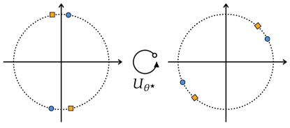
Figure 5: Example of a case where the unsupervised losses could decrease the mAP.

Appendix C Proofs

We now give self-contained proofs of Theorems 3.1 and 3.2.

C.1 Proof of Theorem 3.1

Proof:  Let $f:\mathbb{R}^{k}\to\mathbb{R}^{k}$ be such that $\langle f(u),f(v)\rangle=\langle u,v\rangle$ for all $u,v\in\mathbb{R}^{k}$. Given $\lambda\in\mathbb{R}$ and $u,v\in\mathbb{R}^{k}$ we have that:

$$\begin{split}\|\lambda f(u)-f(\lambda u)\|^{2}&=\lambda^{2}\|f(u)\|^{2}+\|f(\lambda u)\|^{2}\\ &-2\langle\lambda f(u),f(\lambda u)\rangle\\ &=2\lambda^{2}\|u\|^{2}-2\lambda^{2}\langle u,u\rangle\\ &=0.\end{split}$$ (C.1)

Also, note that

$$\begin{split}\|f(u+v)-&f(u)-f(v)\|^{2}\\ &=\|f(u+v)\|^{2}+\|f(u)+f(v)\|^{2}\\ &\,\,\,\,\,\,-2\langle f(u+v),f(u)+f(v)\rangle\\ &=\|u+v\|^{2}+\|u\|^{2}+\|v\|^{2}+2\langle u,v\rangle\\ &\,\,\,\,\,\,-2\left(\langle u+v,u\rangle+\langle u+v,v\rangle\right)\\ &=2\|u+v\|^{2}-2\|u+v\|^{2}\\ &=0.\end{split}$$ (C.2)

This shows that $f$ is linear. The fact that it is orthogonal follows by the fact the it preserves inner products.  $\Box$

C.2 Proof of Theorem 3.2

For Theorem 3.2 we follow [52] and [18]:

Proof:

Given $x\in\mathbb{R}^{k}\setminus\{0\}$, if we take

$$H=I_{k}-2\frac{vv^{T}}{\|v\|_{2}^{2}}$$ (C.3)

with $v=x-\|x\|_{2}e_{1}$, where $e_{1}=(1,0,\ \dots,0)^{T}$, we have

$$Hx=\|x\|_{2}e_{1}.$$ (C.4)

It follows from this that we can transform any $k\times k$ invertible matrix $A$ into an upper-triangular matrix using successive multiplications by Householder matrices. In particular, given $U$ an orthogonal matrix there exists $H_{1},\dots,H_{k-1}$ Householder matrices such that:

$$H_{k-1}\cdots H_{1}U=R,$$ (C.5)

where $R$ is upper-triangular. Since each term on the product on the left hand side of (C.5) is an orthogonal matrix, it follows that $R$ must also be orthogonal, thus $R^{T}R=I_{k}$. Letting $r_{i}$ denote the $i$-th column of $R$, this implies that $\|r_{1}\|^{2}=r^{2}_{11}=1$ so $r_{11}=\pm 1$. Also, $\langle r_{j},r_{1}\rangle=r_{j1}r_{11}=0$ for $j=2,\dots,k$ so $r_{j1}=0$ for $j=2,\dots,k$ since $r_{11}\neq 0$. Repeating this reasoning for the second column and so on we have that $R$ must be diagonal with entries $\pm 1$. We will naturally have that $r_{ii}=1$ for $i=1,\dots,k-1$ by the construction of $H_{i}$. If $r_{kk}=-1$, we do an additional multiplication by $H_{k}=I_{k}-2e^{T}_{k}e_{k}$. Taking $H_{k}=I_{k}$ in case $r_{kk}=1$, it follows that we can write:

$$I_{k}=H_{k}\dots H_{1}U.$$

Since each $H_{i}$ is symmetric and orthogonal, it follows that:

$$H_{1}\dots H_{k}=U.$$

The fact that each product of Householder matrices is orthogonal follows directly from the fact that each Householder matrix is orthogonal and $O(k)$ is closed under multiplications.  $\Box$

References

- [1] P.A. Absil, R. Mahony and R. Sepulchre “Optimization Algorithms on Matrix Manifolds” Princeton University Press, 2009 URL: https://books.google.com.br/books?id=NSQGQeLN3NcC
- [2] Alexandr Andoni, Piotr Indyk, Huy L Nguyen and Ilya Razenshteyn “Beyond locality-sensitive hashing” In Proceedings of the twenty-fifth annual ACM-SIAM symposium on Discrete algorithms, 2014, pp. 1018–1028 SIAM
- [3] Nicolas Aziere and Sinisa Todorovic “Ensemble deep manifold similarity learning using hard proxies” In Proceedings of the IEEE/CVF Conference on Computer Vision and Pattern Recognition, 2019, pp. 7299–7307
- [4] Jane Bromley, Isabelle Guyon, Yann LeCun, Eduard Säckinger and Roopak Shah “Signature verification using a" siamese" time delay neural network” In Advances in neural information processing systems 6, 1993
- [5] A.E. Brouwer and T. Verhoeff “An updated table of minimum-distance bounds for binary linear codes” In IEEE Transactions on Information Theory 39.2, 1993, pp. 662–677 DOI: 10.1109/18.212301
- [6] Yue Cao, Mingsheng Long, Bin Liu and Jianmin Wang “Deep cauchy hashing for hamming space retrieval” In Proceedings of the IEEE Conference on Computer Vision and Pattern Recognition, 2018, pp. 1229–1237
- [7] Zhangjie Cao, Mingsheng Long, Jianmin Wang and Philip S Yu “Hashnet: Deep learning to hash by continuation” In Proceedings of the IEEE international conference on computer vision, 2017, pp. 5608–5617
- [8] Zhangjie Cao, Ziping Sun, Mingsheng Long, Jianmin Wang and Philip S Yu “Deep priority hashing” In Proceedings of the 26th ACM international conference on Multimedia, 2018, pp. 1653–1661
- [9] Yaxiong Chen and Xiaoqiang Lu “Deep discrete hashing with pairwise correlation learning” In Neurocomputing 385 Elsevier, 2020, pp. 111–121
- [10] Sumit Chopra, Raia Hadsell and Yann LeCun “Learning a similarity metric discriminatively, with application to face verification” In 2005 IEEE computer society conference on computer vision and pattern recognition (CVPR’05) 1, 2005, pp. 539–546 IEEE
- [11] Tat-Seng Chua, Jinhui Tang, Richang Hong, Haojie Li, Zhiping Luo and Yantao Zheng “Nus-wide: a real-world web image database from national university of singapore” In Proceedings of the ACM international conference on image and video retrieval, 2009, pp. 1–9
- [12] Tat-Seng Chua, Jinhui Tang, Richang Hong, Haojie Li, Zhiping Luo and Yantao Zheng “Nus-wide: a real-world web image database from national university of singapore” In Proceedings of the ACM international conference on image and video retrieval, 2009, pp. 1–9
- [13] Jia Deng, Wei Dong, Richard Socher, Li-Jia Li, Kai Li and Li Fei-Fei “ImageNet: A large-scale hierarchical image database” In 2009 IEEE Conference on Computer Vision and Pattern Recognition, 2009, pp. 248–255 DOI: 10.1109/CVPR.2009.5206848
- [14] Jia Deng, Wei Dong, Richard Socher, Li-Jia Li, Kai Li and Li Fei-Fei “Imagenet: A large-scale hierarchical image database” In 2009 IEEE conference on computer vision and pattern recognition, 2009, pp. 248–255 Ieee
- [15] Khoa D Doan, Peng Yang and Ping Li “One loss for quantization: Deep hashing with discrete wasserstein distributional matching” In Proceedings of the IEEE/CVF Conference on Computer Vision and Pattern Recognition, 2022, pp. 9447–9457
- [16] Lixin Fan, Kam Woh Ng, Ce Ju, Tianyu Zhang and Chee Seng Chan “Deep Polarized Network for Supervised Learning of Accurate Binary Hashing Codes.” In IJCAI, 2020, pp. 825–831
- [17] Aristides Gionis, Piotr Indyk and Rajeev Motwani “Similarity search in high dimensions via hashing” In Vldb 99.6, 1999, pp. 518–529
- [18] G.H. Golub and C.F. Van Loan “Matrix Computations”, Johns Hopkins Studies in the Mathematical Sciences Johns Hopkins University Press, 1996 URL: https://books.google.com.br/books?id=mlOa7wPX6OYC
- [19] Yunchao Gong, Svetlana Lazebnik, Albert Gordo and Florent Perronnin “Iterative quantization: A procrustean approach to learning binary codes for large-scale image retrieval” In IEEE transactions on pattern analysis and machine intelligence 35.12 IEEE, 2012, pp. 2916–2929
- [20] Jiun Tian Hoe, Kam Woh Ng, Tianyu Zhang, Chee Seng Chan, Yi-Zhe Song and Tao Xiang “One loss for all: Deep hashing with a single cosine similarity based learning objective” In Advances in Neural Information Processing Systems 34, 2021, pp. 24286–24298
- [21] Omid Jafari, Preeti Maurya, Parth Nagarkar, Khandker Mushfiqul Islam and Chidambaram Crushev “A survey on locality sensitive hashing algorithms and their applications” In arXiv preprint arXiv:2102.08942, 2021
- [22] Herve Jegou, Matthijs Douze and Cordelia Schmid “Hamming embedding and weak geometric consistency for large scale image search” In Computer Vision–ECCV 2008: 10th European Conference on Computer Vision, Marseille, France, October 12-18, 2008, Proceedings, Part I 10, 2008, pp. 304–317 Springer
- [23] Hervé Jégou, Matthijs Douze, Cordelia Schmid and Patrick Pérez “Aggregating local descriptors into a compact image representation” In 2010 IEEE computer society conference on computer vision and pattern recognition, 2010, pp. 3304–3311 IEEE
- [24] Qing-Yuan Jiang and Wu-Jun Li “Asymmetric deep supervised hashing” In Proceedings of the AAAI conference on artificial intelligence 32.1, 2018
- [25] Rong Kang, Yue Cao, Mingsheng Long, Jianmin Wang and Philip S Yu “Maximum-margin hamming hashing” In Proceedings of the IEEE/CVF international conference on computer vision, 2019, pp. 8252–8261
- [26] Sungyeon Kim, Dongwon Kim, Minsu Cho and Suha Kwak “Proxy anchor loss for deep metric learning” In Proceedings of the IEEE/CVF conference on computer vision and pattern recognition, 2020, pp. 3238–3247
- [27] Diederik P Kingma and Jimmy Ba “Adam: A method for stochastic optimization” In arXiv preprint arXiv:1412.6980, 2014
- [28] Alex Krizhevsky and Geoffrey Hinton “Learning multiple layers of features from tiny images” Toronto, ON, Canada, 2009
- [29] Alex Krizhevsky, Vinod Nair and Geoffrey Hinton “The CIFAR-10 dataset” In online: http://www. cs. toronto. edu/kriz/cifar. html 55.5, 2014
- [30] Alex Krizhevsky, Ilya Sutskever and Geoffrey E Hinton “Imagenet classification with deep convolutional neural networks” In Advances in neural information processing systems 25, 2012
- [31] Alex Krizhevsky, Ilya Sutskever and Geoffrey E Hinton “Imagenet classification with deep convolutional neural networks” In Advances in neural information processing systems 25, 2012
- [32] Brian Kulis “Metric learning: A survey” In Foundations and Trends® in Machine Learning 5.4 Now Publishers, Inc., 2013, pp. 287–364
- [33] Hanjiang Lai, Yan Pan, Ye Liu and Shuicheng Yan “Simultaneous feature learning and hash coding with deep neural networks” In Proceedings of the IEEE conference on computer vision and pattern recognition, 2015, pp. 3270–3278
- [34] Mario Lezcano Casado “Trivializations for gradient-based optimization on manifolds” In Advances in Neural Information Processing Systems 32, 2019
- [35] Jun Li, Li Fuxin and Sinisa Todorovic “Efficient riemannian optimization on the stiefel manifold via the cayley transform” In arXiv preprint arXiv:2002.01113, 2020
- [36] Wu-Jun Li, Sheng Wang and Wang-Cheng Kang “Feature learning based deep supervised hashing with pairwise labels” In arXiv preprint arXiv:1511.03855, 2015
- [37] Wu-Jun Li, Sheng Wang and Wang-Cheng Kang “Feature learning based deep supervised hashing with pairwise labels” In arXiv preprint arXiv:1511.03855, 2015
- [38] Qi Li, Zhenan Sun, Ran He and Tieniu Tan “Deep supervised discrete hashing” In Advances in neural information processing systems 30, 2017
- [39] Tsung-Yi Lin, Michael Maire, Serge Belongie, James Hays, Pietro Perona, Deva Ramanan, Piotr Dollár and C Lawrence Zitnick “Microsoft coco: Common objects in context” In Computer Vision–ECCV 2014: 13th European Conference, Zurich, Switzerland, September 6-12, 2014, Proceedings, Part V 13, 2014, pp. 740–755 Springer
- [40] Tsung-Yi Lin, Michael Maire, Serge Belongie, James Hays, Pietro Perona, Deva Ramanan, Piotr Dollár and C Lawrence Zitnick “Microsoft coco: Common objects in context” In Computer Vision–ECCV 2014: 13th European Conference, Zurich, Switzerland, September 6-12, 2014, Proceedings, Part V 13, 2014, pp. 740–755 Springer
- [41] Haomiao Liu, Ruiping Wang, Shiguang Shan and Xilin Chen “Deep supervised hashing for fast image retrieval” In Proceedings of the IEEE conference on computer vision and pattern recognition, 2016, pp. 2064–2072
- [42] Wei Liu, Cun Mu, Sanjiv Kumar and Shih-Fu Chang “Discrete graph hashing” In Advances in neural information processing systems 27, 2014
- [43] Wei Liu, Jun Wang, Rongrong Ji, Yu-Gang Jiang and Shih-Fu Chang “Supervised hashing with kernels” In 2012 IEEE conference on computer vision and pattern recognition, 2012, pp. 2074–2081 IEEE
- [44] Wei Liu, Jun Wang, Sanjiv Kumar and Shih-Fu Chang “Hashing with graphs”, 2011
- [45] Xiao Luo, Haixin Wang, Daqing Wu, Chong Chen, Minghua Deng, Jianqiang Huang and Xian-Sheng Hua “A Survey on Deep Hashing Methods” In ACM Trans. Knowl. Discov. Data 17.1 New York, NY, USA: Association for Computing Machinery, 2023 DOI: 10.1145/3532624
- [46] Alexander Mathiasen, Frederik Hvilshoj, Jakob Rodsgaard Jorgensen, Anshul Nasery and Davide Mottin “What If Neural Networks had SVDs?” In NeurIPS, 2020
- [47] Fumin Shen, Chunhua Shen, Wei Liu and Heng Tao Shen “Supervised discrete hashing” In Proceedings of the IEEE conference on computer vision and pattern recognition, 2015, pp. 37–45
- [48] Karen Simonyan and Andrew Zisserman “Very deep convolutional networks for large-scale image recognition” In arXiv preprint arXiv:1409.1556, 2014
- [49] Karen Simonyan and Andrew Zisserman “Very deep convolutional networks for large-scale image recognition” In arXiv preprint arXiv:1409.1556, 2014
- [50] Avantika Singh and Shaifu Gupta “Learning to hash: A comprehensive survey of deep learning-based hashing methods” In Knowledge and Information Systems 64.10 Springer, 2022, pp. 2565–2597
- [51] Rong-Cheng Tu, Xian-Ling Mao, Cihang Kong, Zihang Shao, Ze-Lin Li, Wei Wei and Heyan Huang “Weighted gaussian loss based hamming hashing” In Proceedings of the 29th ACM International Conference on Multimedia, 2021, pp. 3409–3417
- [52] Frank Uhlig “Constructive ways for generating (generalized) real orthogonal matrices as products of (generalized) symmetries” In Linear Algebra and its Applications 332 Elsevier, 2001, pp. 459–467
- [53] Jingdong Wang, Ting Zhang, Nicu Sebe and Heng Tao Shen “A survey on learning to hash” In IEEE transactions on pattern analysis and machine intelligence 40.4 IEEE, 2017, pp. 769–790
- [54] Jun Wang, Sanjiv Kumar and Shih-Fu Chang “Semi-supervised hashing for scalable image retrieval” In 2010 IEEE Computer Society Conference on Computer Vision and Pattern Recognition, 2010, pp. 3424–3431 IEEE
- [55] Qifan Wang, Luo Si and Bin Shen “Learning to hash on structured data” In Proceedings of the AAAI Conference on Artificial Intelligence 29.1, 2015
- [56] Yair Weiss, Antonio Torralba and Rob Fergus “Spectral hashing” In Advances in neural information processing systems 21, 2008
- [57] Rongkai Xia, Yan Pan, Hanjiang Lai, Cong Liu and Shuicheng Yan “Supervised hashing for image retrieval via image representation learning” In Proceedings of the AAAI conference on artificial intelligence 28.1, 2014
- [58] Chengyin Xu, Zenghao Chai, Zhengzhuo Xu, Chun Yuan, Yanbo Fan and Jue Wang “HyP2 Loss: Beyond Hypersphere Metric Space for Multi-Label Image Retrieval” In Proceedings of the 30th ACM International Conference on Multimedia, MM ’22 Lisboa, Portugal: Association for Computing Machinery, 2022, pp. 3173–3184 DOI: 10.1145/3503161.3548032
- [59] Chengyin Xu, Zenghao Chai, Zhengzhuo Xu, Chun Yuan, Yanbo Fan and Jue Wang “Hyp2 loss: Beyond hypersphere metric space for multi-label image retrieval” In Proceedings of the 30th ACM International Conference on Multimedia, 2022, pp. 3173–3184
- [60] Li Yuan, Tao Wang, Xiaopeng Zhang, Francis EH Tay, Zequn Jie, Wei Liu and Jiashi Feng “Central similarity quantization for efficient image and video retrieval” In Proceedings of the IEEE/CVF conference on computer vision and pattern recognition, 2020, pp. 3083–3092
- [61] Hanwang Zhang, Na Zhao, Xindi Shang, Huanbo Luan and Tat-seng Chua “Discrete image hashing using large weakly annotated photo collections” In Proceedings of the AAAI Conference on Artificial Intelligence 30.1, 2016
- [62] Zheng Zhang, Qin Zou, Yuewei Lin, Long Chen and Song Wang “Improved Deep Hashing With Soft Pairwise Similarity for Multi-Label Image Retrieval” In IEEE Transactions on Multimedia 22.2, 2020, pp. 540–553 DOI: 10.1109/TMM.2019.2929957
- [63] Han Zhu, Mingsheng Long, Jianmin Wang and Yue Cao “Deep hashing network for efficient similarity retrieval” In Proceedings of the AAAI conference on Artificial Intelligence 30.1, 2016