Elastic and resonance structures of the nucleon from hadronic tensor in lattice QCD: implications for neutrino-nucleon scattering and hadron physics

Abstract

Understanding the transitions of nucleons into various resonance structures through electromagnetic interactions plays a pivotal role in advancing our comprehension of the strong interactions within the domain of quark confinement. Furthermore, gaining precise insights into the elastic and resonance structures of nucleons is indispensable for deciphering the physics from neutrino-nucleus scattering cross sections experimental data, which remain theoretically challenging, even in the context of neutrino-nucleon interactions whose profound understanding is imperative for the neutrino oscillation experiments. One promising avenue involves the direct evaluation of the lepton-nucleon scattering cross sections across quasi-elastic, resonance, shallow-inelastic, and deep inelastic regions, which can be achieved through the hadronic tensor formalism in lattice QCD. In this work, we present the determination of the nucleon’s Sachs electric form factor using the hadronic tensor formalism and verify that it is consistent with that from the conventional three-point function calculation. We additionally obtain the transition form factor from the nucleon to its first radial excited state within a finite volume. Consequently, we identify the latter with the nucleon-to-Roper transition form factor $G_{E}^{*}(Q^{2})$, determine the corresponding longitudinal helicity amplitude $S_{1/2}(Q^{2})$ and compare our findings with experimental measurements, for the first time using the hadronic tensor formalism. The limitations and systematic improvements of the approach are also discussed.

I Introduction

Understanding the hadronic tensor occupies a central and indispensable role in the domains of particle and nuclear physics through its relevance in quasi-elastic, resonance, and deep inelastic scattering experiments. A profound knowledge of hadronic tensors is essential to discern valuable information about the internal structure of hadrons and the distribution of quarks and gluons within hadrons, and to gain insights into the strong interactions. Lattice quantum chromodynamics (QCD) determinations of the hadronic tensor [1, 2] offer an opportunity to significantly influence our comprehension of the neutrino-nucleon interactions and can provide valuable complementary theoretical constraints while interpreting data from the neutrino oscillation experiments. Furthermore, understanding the excitation spectrum of baryons and mesons, as well as characterizing the effective degrees of freedom in various QCD coupling regimes, stand as some of the most important and undeniably challenging endeavors within the field of hadronic physics where hadronic tensor can provide direct information on these transition spectra and spectral weights. The potential of this approach was promptly acknowledged in the white papers relevant to neutrino physics [3, 4]. It was highlighted that the scattering cross-section for neutrino-nucleon ($\nu-N$) interactions can be obtained by utilizing both the leptonic and hadronic tensors, with the nonperturbative hadronic tensor computable through the first-principles lattice QCD calculations.

The investigation of the hadronic tensor within lattice QCD will offer a significant influence on our comprehension of the findings from the Deep Underground Neutrino Experiment (DUNE) [5] and Hyper-K [6] experiments. Neutrino oscillation experiments are performed using scattering on nuclear targets, and it is crucial to construct appropriate models for neutrino-nucleus ($\nu-A$) interactions, which involve modifications to $\nu-N$ interactions due to nuclear effects. These model buildings are essential to effectively analyze the data and accurately reproduce and interpret the observed cross sections, enabling the investigation of neutrino oscillations. This task requires the direct incorporation of scattering amplitudes at the nucleon level. Gaining precise knowledge of the $\nu-N$ scattering cross-section within the few-GeV range is indispensable for exploring charge-parity (CP) symmetry violation in the leptonic sector. Furthermore, the total cross sections for $\nu-N$ or $\nu-A$ scattering at various neutrino beam energies are due to contributions from quasi-elastic (QE), resonance (RES), shallow inelastic (SIS), and deep inelastic scattering (DIS) processes, as discussed in [7]. At energies below $1$ GeV, in which a nucleon is knocked out of the target nucleus, QE scattering ($\nu_{l}+n\to l^{-}+p$, $\overline{\nu}_{l}+p\to l^{+}+n$) primarily governs the scattering cross-section, which can be derived using the hadronic tensor formalism. On the contrary, within the RES, SIS, and DIS energy ranges, the cross section incorporates inputs from inelastic neutrino-nucleon interactions. In the region of resonant pion production, the contribution of the $\Delta$-resonance to the neutrino cross section is the most prominent one. However, the contributions coming from the second resonance region, which includes three isospin-$\frac{1}{2}$ states: $D_{13}(1520),~{}P_{11}(1440)$ and $S_{11}(1535)$, are also important.

This necessitates the determination of the hadronic tensor to encompass all-inclusive contributions, information that can be obtained from lattice QCD calculations. However, grasping the entirety of the resonant region, which encompasses a spectrum of multi-particle states, poses a formidable challenge. Yet, there is promise in reconstructing these spectral functions through the use of two currents in different channels, enabling the computation of the inclusive hadronic tensor. Furthermore, the SIS region, situated between resonances and deep inelastic scattering, currently lacks a consistent theoretical model for its description [8]. It is likely that future calculations of the hadronic tensor in the SIS region will offer valuable theoretical insights, as suggested in [3]. The desired precision for these measurements, encompassing systematic uncertainties (which presently dominate the pursuit of physics discoveries), lies within the range of $1-4\%$ for the $\nu_{\mu}\to\nu_{e}$ and $\bar{\nu}_{\mu}\to\bar{\nu}_{e}$ oscillation probabilities [8, 3, 4]. Hence, the imperative of directly determining the hadronic tensor through lattice QCD becomes essential to fully harness the potential of new neutrino experimental facilities such as DUNE and Hyper-K.

For instance, in [9], lattice QCD inputs of the strange quark form factors and strange quark contribution to nucleon spin from [10, 11, 12, 13] were utilized. These were then combined with experimental measurements of neutrino-nucleon scattering differential cross sections [14, 15], without considering nuclear effects, in order to determine the neutral current weak axial form factor that remains largely unknown. Conversely, the ultimate objective is to directly determine nucleon-level structure functions crucial for neutrino scattering cross sections from lattice QCD. In this regard, in an ideal scenario where all systematic uncertainties are well-controlled, the computation of the hadronic tensor through lattice QCD can provide predictions for nucleon-level structure functions, encompassing various types of current combinations, such as vector-vector, vector-axial, and axial-axial currents. While the lattice QCD formalism of the hadronic tensor formalism [1, 2] demands considerable computational resources [16] and poses several numerical challenges, the selection of two currents at two different spacetime locations on the lattice provides an opportunity to regulate and achieve desired overlaps into exclusive channels. This contrasts with the real-world experiments where contributions from various channels overlap in a complicated manner, making their disentanglement challenging. The nucleon-level structure functions originating from these different channels from the hadronic tensor are vital and can be integrated into neutrino event generators for building nuclear many-body theory to investigate $\nu-A$ scattering structure functions [4, 17].

The formalism of the hadronic tensor also facilitates the exploration of nucleon resonance excitations that manifest through intermediate processes like $\gamma N\to N^{*}$. Consequently, this approach enables the determination of cross sections in terms of electromagnetic transition form factors or helicity transition amplitudes. Such an application of the hadronic tensor offers useful information to investigate baryon resonances via electromagnetic excitations [18] and the exclusive electroproduction of mesons involving baryon resonances [19] which is directly related to the experimental program of the determination of generalized parton distributions (GPDs) at Jefferson Lab. While the hadronic tensor formalism in lattice QCD directly allows to determination GPDs, they also provide complementary information in the GPD program through their access to the resonance transition form factors. The investigation of nucleon resonances stands as a significant objective for the CEBAF Large Acceptance Spectrometer (CLAS) at Jefferson Lab, as well as for lattice QCD spectroscopy programs [20]. Notably, a comprehensive understanding of the nucleon resonance excitation within electromagnetic interactions yields crucial insights into the dynamics of strong interactions within the realm of quark confinement [21]. In addition, the determination of the transition amplitudes in a wide range of momentum transfer allows to map out the quark transverse charge distributions that induce these transitions [22, 23, 21]. Notably, the hadronic tensor formalism [1, 2] also allows one to determine the $x$-dependent structure functions, being complementary to other lattice QCD formalisms proposed in [24, 25, 26, 27, 28, 29].

It is worth mentioning that the initial proposals of the hadronic tensor [30, 31] allowed for the study of connected and disconnected sea partons, thereby realizing the violation of the Gottfried sum rule [32] in [1, 33]. Additionally, by numerically computing different topologies of the quark lines in the four-point current-current correlator, the hadronic tensor enables the direct estimation of contributions from higher-twist “cat’s ears” diagrams, as well as the leading-twist “hand-bag” diagram in the DIS processes. This opens up an avenue for studying higher-twist contributions in DIS processes from first principles, which are usually estimated through some parametrization in phenomenological studies and global fits. Such a calculation using the Compton amplitude formalism can be found in [34] and an exploratory calculation using the hadronic tensor formalism can be found in [35].

Considering the promising implications for physics, we commence by outlining the distinctive advantages of computing the hadronic tensor through lattice QCD and point out some comparisons and its complementarity with other lattice formalisms in Sec. II. Subsequently, we will delve into the challenges associated with extracting physics information in Minkowski space. In Sec. III, we briefly discuss the hadronic tensor formalism and its implementation on the lattice in Sec. IV. We provide details of the extraction of the matrix elements for the elastic (both using the conventional three-point function and hadronic tensor formalism) and transition form factors in Sec. V and draw comparisons with the experimental data. In Sec. VI, we highlight forthcoming directions, along with potential theoretical uncertainties and limitations associated with the current method, all aimed at attaining the precision goal in future calculations and then conclude our paper.

II Unique features and challenges in computing hadronic tensor

One significantly important aspect of the simplicity of the hadronic tensor formalism [1, 2] is that the hadronic tensor is scale-independent and the structure functions are frame-independent. Unlike several technical challenges associated with renormalizing the equal-time matrix elements of bilocal operators in quasi [25] and pseudo [28] PDFs approaches, which have received considerable attention in recent years [36, 37, 24, 38, 39], the lattice QCD calculation of the hadronic tensor offers unique advantages in that it does not necessitate renormalization stemming from spatial Wilson line operators.

There are several lattice QCD formalisms involving two-currents. Notably, a noteworthy distinction between the hadronic tensor and the spatially-separated two-currents approach [40, 41, 42, 29, 43, 44, 45] lies in the fact that the hadronic tensor involves two currents that are both spatially and temporally separated. On the other hand, the Compton amplitude approach [27, 46] also employs two currents at different spacetime points, akin to the hadronic tensor, but it computes the lattice matrix elements in the unphysical region, suppressing the intermediate states between the two currents from going on-shell. Conversely, the hadronic tensor in our work is evaluated in the physical region where the intermediate states are physical.

The insertion of two currents in the evaluation of the hadronic tensor on the lattice involves a Euclidean temporal separation, which presents a major challenge: converting the lattice-calculated hadronic tensor from Euclidean space to Minkowski space. This conversion poses a formidable inverse problem, notable not only for the challenges arising from the discrete nature of data and its limited quantity but also for the intricacies involved in constructing the spectral density encompassing various elastic, inelastic scatterings, and resonance structures that collectively contribute to the hadronic tensor. However, it offers a unique opportunity to directly probe the physics of intermediate states that propagate between the currents, enabling the study of transitions from the nucleon to its various resonance states. Additionally, it is important to note that elastic and resonance structures are significantly suppressed in the DIS region. When analyzed within the DIS framework, the hadronic formalism provides an alternative avenue for investigating the nucleon’s partonic structure. This approach complements lattice QCD calculations conducted through different methodologies, where substantial progress has already been achieved (for many recent developments and results, see [47, 48, 49, 50] and the references therein). In principle, the hadronic tensor serves as a framework that enables the investigation of hadron structure across the elastic, resonance, and DIS regions, including the challenging transition regions that lie in between them.

III Calculation of elastic and transition form factors from hadronic tensor formalism on the lattice

The response of the target nucleon to the photon probe is characterized by a hadronic tensor. The hadronic tensor involved in the inclusive lepton-nucleon scattering cross section is the imaginary part of the Compton amplitude $T_{\mu\nu}$ and can be written in the following form for spin-averaged nucleon states:

$$W_{\mu\nu}(q^{2},\nu)=\frac{1}{\pi}T_{\mu\nu}(q^{2},\nu)=\frac{1}{2}\sum_{n}\int\prod_{i=1}^{n}\bigg{[}\frac{\differential^{3}p_{i}}{(2\pi)^{3}2Ep_{i}}\bigg{]}\bra{N(p)}J_{\mu}(0)\ket{n}\bra{n}J_{\nu}(0)\ket{N(p)}(2\pi)^{3}\delta^{4}(p_{n}-p-q),$$ (1)

where $p$ and $p_{n}$ are the 4-momentum of the nucleon and $n$-th intermediate states, $q$ is the momentum transfer ($q^{2}=-Q^{2}$), and $\nu$ is the energy transfer. Being an inclusive reaction, the hadronic tensor in the lepton-nucleon scattering includes all intermediate states as shown in Eq. (1). $W_{\mu\nu}$ cannot be calculated in perturbation theory. It parametrizes our ignorance of the nucleon when analyzing experimentally measured cross sections.

Formally, the hadronic tensor formalism expressed as in Eq. (1), can be obtained in the Euclidean space by calculating a four-point correlation of two currents on the lattice. This Euclidean hadronic tensor $W^{E}_{\mu\nu}$ can be converted into the hadronic tensor in Minkowski space $W^{M}_{\mu\nu}$ by employing the inverse Laplace transform, wherein $\tau$ is treated as a continuous dimensionful variable:

$$W^{M}_{\mu\nu}(\vec{p},\vec{q},\nu)=\frac{1}{2m_{N}i}\int_{c-i\infty}^{c+i\infty}\differential\tau\,e^{\nu\tau}W^{E}_{\mu\nu}(\vec{p},\vec{q},\tau),$$ (2)

with $c>0$. However, since there is no lattice data at imaginary $\tau$, it is not a feasible approach to execute the transformation as indicated in Eq. (2). On the other hand, this can be cast into an inverse problem in the form of a Laplace transform [51]:

$$W^{E}_{\mu\nu}(\vec{p},\vec{q},\tau)=\int\differential\nu~{}e^{-\nu\tau}W^{M}_{\mu\nu}(\vec{p},\vec{q},\nu)$$ (3)

However, in this work, we are interested in the nucleon elastic form factor and the transition form factor of the first radial excitation in the finite volume. In order to extract these form factors or structure functions, it is necessary to evaluate the nucleon two-point (2pt) and four-point (4pt) correlation functions. We can start by expressing the 2pt correlation function as follows:

$$C^{2{\rm pt}}_{\alpha\beta}(\vec{p}_{f}=\vec{p},t_{f},\vec{p}_{i}=\vec{p},t_{0})=\sum_{\vec{x}_{0}}e^{i\vec{p}\cdot\vec{x}_{0}}\sum_{\vec{x}}e^{-i\vec{p}\cdot\vec{x}}\bra{0}\chi^{N}_{\alpha}(\vec{x},t_{f})\overline{\chi}^{N}_{\beta}(\vec{x}_{0},t_{0})\ket{0},$$ (4)

where $\chi^{N}(\overline{\chi}^{N})$ is the nucleon annihilation(creation) interpolation field and $\vec{p}_{i},x_{0},t_{0}$ and $\vec{p}_{f},x,t_{f}$ are nucleon momenta, spatial, and temporal positions of the source and sink, respectively. In the limit where $(t_{f}-t_{0})$ is large, taking the trace for positive parity projection, we can write

$$\Tr(\Gamma_{e}G^{2{\rm pt}})(\vec{p}_{f},t_{f},\vec{p}_{i},t_{0})\xrightarrow[]{(t_{f}-t_{0})\gg 0}\overline{Z}_{i}Z_{f}\frac{(E_{N,\vec{p}}+m_{N})}{E_{N,\vec{p}}}e^{-E_{N,\vec{p}}(t_{f}-t_{0})},$$ (5)

where $Z$ is the transition matrix element $\bra{0}\chi^{N}\ket{N}$ and $\Gamma_{e}=(1+\gamma_{4})/2$. The Euclidean hadronic tensor $W^{E}_{\mu\nu}$ can be constructed from the following 4pt correlation function with current insertions at two different space-time positions $(\vec{x}_{2},t_{2})$ and $(\vec{0},t_{1})$ and momentum transfer $\vec{q}$ between the currents. The nucleon 4pt correlation function can be written as:

$$C^{4{\rm pt}}_{\alpha\beta}(\vec{p}_{f}=\vec{p},t_{f},\vec{q},t_{2},t_{1},\vec{p}_{i}=\vec{p},t_{0})=\sum_{\vec{x}_{0}}e^{i\vec{p}\cdot\vec{x}_{0}}\sum_{\vec{x}}e^{-i\vec{p}\cdot\vec{x}}\bra{0}\chi^{N}_{\alpha}(\vec{x},t_{f})\sum_{\vec{x}_{2}}e^{-i\vec{q}\cdot\vec{x}_{2}}J_{\mu}(\vec{x}_{2},t_{2})J_{\nu}(\vec{0},t_{1})\overline{\chi}^{N}_{\beta}(\vec{x}_{0},t_{0})\ket{0}.$$ (6)

The current associated with the matrix element of the nucleon form factors in the elastic region can be parameterized in terms of the Dirac $F_{1}$, and Pauli $F_{2}$, form factors:

$$\bra{N(p)}J_{\mu}\ket{N(p^{\prime})}=\bar{u}(p)[\gamma_{\mu}F_{1}(-q^{2})-\sigma_{\mu\nu}q_{\nu}\frac{F_{2}(-q^{2})}{2m}]u(p^{\prime}),$$ (7)

where $q=p-p^{\prime}$, $\sigma_{\mu\nu}=\frac{1}{2i}[\gamma_{\mu},\gamma_{\nu}]$. Here all the matrices are in Euclidean notation and we will also continue using these notations in the subsequent parts of the calculation. On the other hand, a Lorentz decomposition of the $\gamma^{*}N\to N^{*}$ transition matrix element associated with the electromagnetic current can be written as [52, 23, 53]:

$$\bra{N^{*}(p)}J_{\mu}\ket{N{(p^{\prime})}}=\bar{u}_{N^{*}}(p)\bigg{[}(\gamma_{\mu}-\frac{q_{\mu}\not{q}}{q^{2}})F^{*}_{1}(-q^{2})-\frac{\sigma_{\mu\alpha}q_{\alpha}}{m_{N}+m^{*}}F^{*}_{2}(-q^{2})\bigg{]}u_{N}(p^{\prime}).$$ (8)

Note that the structure of the current, which closely resembles its nucleonic counterpart, with the exception of the $q_{\mu}\not{q}$ component. In the case of the nucleon, the form factor related to this operator must vanish to maintain current conservation. However, this requirement does not hold for the Roper, given the difference in mass between the nucleon and Roper, with $m^{*}\neq m_{N}$. In this work, we concentrate on the electric form factors, such as the nucleon Sachs electric form factor, $G_{E}$, and the nucleon to its radial excitation electric transition form factor, $G_{E}^{*}$, only. Therefore, we will explicitly choose $\mu=\nu=4$ in the above expressions for currents and matrix elements. In this calculation, we consider the source and sink to be at rest, $\vec{p}_{f}=\vec{p}_{i}=\vec{0}$ and consider various momentum transfers at the currents. For this case, after inserting a complete set of intermediate states and with nucleon-to-nucleon (N-N) and nucleon to its first radial excitation, (N-R) scattering included, we can write Eq. (6) as the following:

$$\begin{aligned} \mathrm{Tr}[\Gamma_{e}G^{\rm 4pt}(\vec{p}_{f}=\vec{0},t_{f},\vec{q},t_{2},t_{1},\vec{p}_{i}=\vec{0},t_{0})]&\xrightarrow[t_{1}\gg t_{0}]{t_{f}\gg t_{2}\gg t_{1}}(\Gamma_{e})_{\beta\alpha}\sum_{m,n,l}\sum_{\vec{s},\vec{s}_{i},\vec{s}_{f}}\bra{0}\chi_{\alpha}^{N}\ket{m,\vec{s}_{f}}\frac{m_{m}m_{n}}{E_{m,\vec{p}_{f}}E_{n,\vec{p}_{i}}}\frac{m_{l}}{E_{l,\vec{q}}}\\ &\quad\quad\quad\quad\quad\times\bra{m,\vec{s}_{f}}J_{\mu}\ket{l,\vec{q},\vec{s}}\bra{l,\vec{q},\vec{s}}J_{\nu}\ket{n,\vec{s}_{i}}\\ &\quad\quad\quad\quad\quad\times\bra{n,\vec{s}_{i}}\overline{\chi}^{N}_{\beta}\ket{0}e^{-E_{n,\vec{q}}(t_{2}-t_{1})}e^{-E_{m,\vec{p}}(t_{f}-t_{2})-E_{n,\vec{p}}(t_{1}-t_{0})}\\ &\xrightarrow[n=m=N]{l=N,R}(\Gamma_{e})_{\beta\alpha}\sum_{\vec{s},\vec{s}_{i},\vec{s}_{f}}\bra{0}\chi_{\alpha}^{N}\ket{N,\vec{s}_{f}}\frac{m_{N}^{2}}{(E_{N,\vec{p}})^{2}}\frac{m_{N}}{(E_{N,\vec{q}})}e^{-E_{N,\vec{p}}(t_{f}-t_{0})}\\ &\quad\quad\quad\quad\quad\times\bra{N,\vec{s}_{f}}J_{\mu}\ket{N,\vec{q},\vec{s}}\bra{N,\vec{q},\vec{s}}J_{\nu}\ket{N,\vec{s}_{f}}\\ &\quad\quad\quad\quad\quad\times\bra{N,\vec{s}_{f}}\overline{\chi}^{N}_{\beta}\ket{0}e^{-(E_{N,\vec{q}}~{}-~{}E_{N,\vec{p}})(t_{2}-t_{1})}\\ &\quad\quad\quad\quad+\sum_{\vec{s},\vec{s}_{i},\vec{s}_{f}}\bra{0}\chi_{\alpha}^{N}\ket{N,\vec{s}_{f}}\frac{m_{N}^{2}}{(E_{N,\vec{p}})^{2}}\frac{m_{R}}{(E_{R,\vec{q}})}e^{-E_{N,\vec{p}}(t_{f}-t_{0})}\\ &\quad\quad\quad\quad\quad\times\bra{N,\vec{s}_{f}}J_{\mu}\ket{R,\vec{q},\vec{s}}\bra{R,\vec{q},\vec{s}}J_{\nu}\ket{N,\vec{s}_{f}}\\ &\quad\quad\quad\quad\quad\times\bra{N,\vec{s}_{f}}\overline{\chi}^{N}_{\beta}\ket{0}e^{-(E_{R,\vec{q}}~{}-~{}E_{N,\vec{p}})(t_{2}-t_{1})}+...\\ &=\overline{Z}_{i}Z_{f}e^{-E_{N,\vec{p}}(t_{f}-t_{0})}\Bigg{\{}\frac{E_{N,\vec{q}}+m_{N}}{E_{q}}G_{E}^{2}e^{-(E_{N,\vec{q}}~{}-~{}E_{N,\vec{p}})\tau}\\ &+\frac{E_{R}+m_{R}}{E_{R}}\bigg{[}\frac{(E_{R}-m_{R})(m_{N}+m_{R})}{q^{2}}\bigg{]}^{2}(G^{*}_{E})^{2}e^{-(E_{R,\vec{q}}~{}-~{}E_{N,\vec{p}})\tau}\Bigg{\}}+...,\end{aligned}$$ (9)

where we have written the temporal dependence of the two currents as a function of Euclidean time separation, $\tau=t_{2}-t_{1}$. Here, we have defined $G_{E}(Q^{2})=F_{1}(Q^{2})-\frac{Q^{2}}{4m_{N}^{2}}F_{2}(Q^{2})$ for the nucleon elastic form factor. Similarly, $G_{E}^{*}(Q^{2})$ can be defined from the matrix element definition (8) as a function of $F_{1}^{*}(Q^{2})$ and $F_{2}^{*}(Q^{2})$. As we will discuss in the numerical details, our lattice has a relatively heavy pion mass at 371 MeV and a lattice size of 1.92 fm. Therefore, the expected first $\pi N$ state is $\sim 200$ MeV higher than the Roper. Thus, we shall not consider the potential $\pi N$ state contribution in the present calculation of the hadronic tensor. The form factors $G_{E}$ and $G_{E}^{*}$ can be determined from the ratio of the nucleon 4pt to 2pt functions and we obtain

$$R^{\rm 4pt/2pt}(\vec{p}_{f}=\vec{0},t_{f},\vec{q},t_{2},t_{1},\vec{p}_{i}=\vec{0},t_{0}) = \frac{1}{2}\Bigg{(}{\frac{E_{N,\vec{q}}+m_{N}}{E_{N,\vec{q}}}}G_{E}^{2}e^{-(E_{N,\vec{q}}~{}-~{}m_{N})\tau}$$ (10)

$$+ \frac{E_{R}+m_{R}}{E_{R}}\bigg{[}\frac{(E_{R}-m_{R})(m_{N}+m_{R})}{q^{2}}\bigg{]}^{2}(G^{*}_{E})^{2}e^{-(E_{R,\vec{q}}~{}-~{}m_{N})\tau}\Bigg{)},$$

where we have used $E_{N,\vec{0}}=m_{N}$. In the following, the mass $m_{R}$ associated with the transition matrix elements will be denoted by $m^{*}$ and various energy differences in Eq. (10) will be denoted by $\Delta E_{n}$.

IV Description of numerical setups

For the numerical calculation of the hadronic tensor on the lattice, one needs to calculate several topologically different diagrams (both the connected insertions and disconnected insertions) as depicted in Fig. 1. Different Wick contractions for the 4pt function lead to these diagrams in the Euclidean path-integral formulation. However, for this calculation, we only concentrate on the connected insertion contributions as depicted in the first row of Fig. 1 and ignore the disconnected insertions (in the second row of Fig. 1).

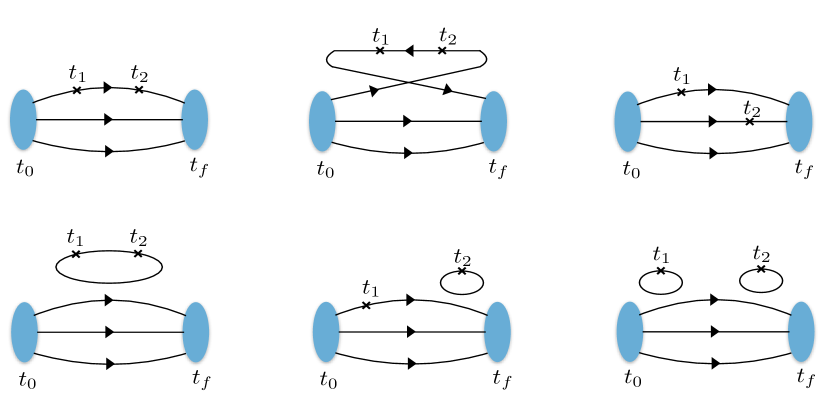
Figure 1: Topologically distinct diagrams in the Euclidean-path integral formulation of the nucleon hadronic tensor. The flavors of the quark lines are not specified in the figure. The first row shows the connected insertion and the second row shows the disconnected insertion contributions.

In general, the Wick contraction in the third column of the first row in Fig. 1, known as the cat’s ear diagram in the DIS jargon describes nonperturbative interactions between the struck quark and the spectator quarks in DIS process. In the DIS, the matrix elements of the cat ear diagram yield contributions of the structure functions that are suppressed by $1/Q^{2}$ and are often ignored. However, as we investigate the QE and RES regions at low energies and low $Q^{2}$, the contribution from this diagram is not negligible [35] and we include it in this calculation.

We adopt similar numerical techniques from the work in Ref. [54] for the lattice QCD implementation of this calculation. Our calculations are conducted on the RBC/UKQCD domain wall lattice, 32Ifine [55], characterized by a lattice spacing of approximately $0.06$ fm. The tadpole improved clover coefficient $c_{\rm sw}=1.033$ is used to generate the clover term of the clover action for the valence quarks. The pion mass is tuned to be close to the unitary point $m_{\pi}=371$ MeV. A fast fermion smearing scheme [56] is employed on both the source and sink sides to enhance the ground-state overlap. We use two sequential propagators for constructing the 4pt correlation function with one starting at the nucleon source location $t_{0}$ through the first current at $t_{1}$ to the second current at $t_{2}$. The second one starts from $t_{0}$ and goes through the nucleon sink position $t_{f}$ to $t_{2}$. Therefore, for each calculation, the source point $t_{0}$ and the two sequential points $t_{1}$ and $t_{f}$ are fixed. This allows us to have variable $t_{2}$ for the second current insertion time. For this calculation, we choose $t_{0}=0$, $t_{1}=4$ and $t_{f}=20$ in the lattice units. We therefore have $t_{2}$ in the range of $0-16$ in lattice units. We also perform the calculation with $t_{1}=5$ and $6$ in the lattice units to investigate the excited-state contamination from the nucleon source to the first current temporal separation. As discussed earlier, since we are interested in the elastic and transition electric form factors, we choose $\mu=\nu=4$ for the choice of currents in Eqs. (7) and (8). We keep the nucleon source and sinks at rest $\vec{p}_{i}=\vec{p}_{f}=\vec{0}$ and insert seven momentum transfers at the currents with $\vec{q}=[(0,0,0),(0,0,1),(0,1,1),(1,1,1),(0,0,2),(0,1,2),(1,1,2)]$ in the lattice units.

V Matrix elements extraction for the elastic and transition form factors

As with any other lattice QCD calculations of the hadron structure, one of the most challenging parts is to reliably extract the desired matrix elements from the nucleon correlation functions. In practice, one can determine the energy spectrum from fits to the 2pt functions, and then feed these results into the 3pt or 4pt function analyses or sometimes use them as a Bayesian prior for the 3pt or 4pt correlation fits. On the other hand, we emphasize that the underlying assumption of the lattice QCD hadronic tensor is that the intermediate states between the currents are induced by the specific currents and lead to overlap on the desired channel of the matrix elements.

In this work, we opt to fit the 4pt/2pt correlation ratio, thereby determining the nucleon mass across various momentum transfers. We then compare these findings with the nucleon mass extracted from the 2pt correlation. On the other hand, in an ideal case, these values of $(E_{R,\vec{q}}~{}-~{}E_{N,\vec{p}})$ and $(E_{N,\vec{q}}~{}-~{}E_{N,\vec{p}})$ depend on the momentum transfer insertion $\vec{q}$ to the currents according to the dispersion relation and the choice of currents. We also investigate if such expectations are achieved in the extraction of the matrix elements.

In what follows, prior to employing the fit to the 4pt/2pt correlation function, we initially employ Bayesian reconstruction (BR) [57] for reconstructing the spectral functions based on the 4pt/2pt correlation. This approach allows us to investigate the energy spectrum and determine the values of spectral function peaks at various $\Delta E_{n}$ values. These results can then be compared with the extraction of $\Delta E_{n}$ values obtained from fitting the 4pt/2pt correlation. Subsequently, we perform exponential fits to the 4pt/2pt correlation and use this as a consistency check, qualitatively comparing the resulting energy spectrum with that obtained through BR.

V.1 Bayesian reconstruction of spectral functions

Bayesian inference can be used to address the ill-posed inverse problem by systematically incorporating additional prior information available. In the context of handling the inverse problem for the two-current correlation, the Backus-Gilbert method [58] was introduced in [59] and [54]. Furthermore, as a Bayesian method, the maximum entropy method [60] was also applied to solve the inverse problem in [54]. It was observed that this method produced a similar outcome for reconstructing the flat spectral region, while qualitatively enhancing the reconstruction of spectral peaks when compared to the Backus-Gilbert method. Additionally, there are proposals in [61, 62] for the reconstruction of smeared spectral functions from Euclidean correlation functions. For example, a formalism in [59] was proposed to determine various transition rates from the nucleon 4pt function calculations by extracting smeared spectral functions from appropriately constructed finite-volume Euclidean correlation functions such that a well-defined infinite-volume limit exists. Reconstructing these smeared spectral functions from Euclidean correlation functions, as proposed in these prior works [59, 61, 62], is an important direction that we plan to investigate in the future. In this study, to assess the consistency of $\Delta E_{n}$ determination between the inversion method and exponential fitting, we will employ Bayesian reconstruction [57]. Previous lattice QCD calculations of the hadronic tensor [54] have demonstrated that the BR method exhibits the highest resolution for extracting peak structures in the low-momentum transfer regions. While the BR method incorporates all the essential properties of the maximum entropy method [60] for reconstructing positive spectral functions from lattice QCD data, it also ensures scale-invariance by enforcing that the posterior does not depend on the units of the spectral function, leading to only ratios between the parameters of interest related to the unknown process and the default model. We briefly discuss the essential features of the BR method in the following and demonstrate its applications on the lattice data. A detailed discussion on the BR method and its comparison with Backus-Gilbert and the maximum entropy method can be found in the latest review article [63].

According to the Bayesian reconstruction method developed in [57] the Bayesian probability is

$$P[\omega|D,\alpha,m]\propto\exp[S_{\rm BR}(\omega)].$$ (11)

Here, $P[\omega|D,\alpha,m]$ is the probability that $\omega$ is the solution given lattice data $D$, $m$ is the prior information (called the default model), and $\alpha$ is a hyper parameter. $\omega=\{\omega_{1},\omega_{2},\cdots,\omega_{l}\}$ denotes a specified combination of the fitted parameters; ${\rm P}({\rm data})$ is called evidence. The essential goal of using Bayesian inference is to get an estimation of the unknown parameters $\omega_{l}$, for example, that govern the generation of the input lattice QCD data, $D_{i}$, and unobserved future data sets. In Eq. (11), the regulator $S_{\rm BR}$ is

$$S_{\rm BR}=\alpha S^{\prime}-L-\gamma(L-N_{\tau})^{2}$$ (12)

and

$$S^{\prime}=\sum_{l}\bigg{[}1-\frac{\omega_{l}(\mu_{l})}{m_{l}(\mu_{l})}+\ln\bigg(\frac{\omega_{l}(\mu_{l})}{m_{l}(\mu_{l})}\bigg{missing})\bigg{]}\Delta\mu_{l}.$$ (13)

In the above equation, $m_{l}$ is the maximum of each normal distribution with the uncertainty of the width equal to $1/\alpha_{l}$, and the Euclidean correlator from the lattice $D_{i}$ is known at $N_{\tau}$ discrete points $\tau_{i}$. In the absence of the simulation data, $m_{l}$ denotes the most probable a priori value of $\omega_{l}$ with intrinsic uncertainty $1/\alpha_{l}$. $\Delta\mu_{l}$ is the width of the discretized lattice data at frequencies $\mu_{l}$ along $N_{\mu}$ equidistant frequency bins. One important feature of the above ratio is that the logarithm requires none of the $\omega_{l}$ and $m_{l}$ be zero. The ratios between the parameters of the unknown process and the default model ensure that the posterior does not depend on the units of the spectral function. $\Delta\mu_{l}$ can be absorbed in the re-definition of $\alpha$ and after integrating out the hyper-parameter $\alpha$, we get,

$$P[\omega|D,m]=\frac{P[D|\omega,I]}{P[D,m]}\int\differential\alpha P[\alpha|D,m],$$ (14)

where $I$ is the prior information and $P[D|\omega,I]$ can be determined in terms of the likelihood function $L$. $L=\frac{1}{2}\sum_{i,j}(c(\tau_{i})-c^{\omega}(\tau_{i}))C^{-1}_{ij}(c(\tau_{j})-c^{\omega}(\tau_{j}))$ is determined with $c^{\omega}(\tau_{i})$ being the correlator reconstructed using $c(\tau_{i})=\sum_{j}k(\tau_{i},\nu_{j})\omega(\nu_{j})\Delta\nu_{j}$ with discretized target function $\omega(\nu)$. Here, $k(\tau_{i},\nu)$ is the integral kernel of $c(\tau_{i})$.

As mentioned above, we can now use the hadronic tensor formalism to extract the form factors from the 4pt/2pt correlation functions. We use the BR method in the following to explore the reconstruction of the spectral weights from these 4pt/2pt correlation functions. Following the functional form in Eq. (10), the ratio of 4pt to 2pt correlation functions can be expressed in the following functional form:

$$\begin{aligned} R^{\rm 4pt/2pt}(\vec{p}_{f}=\vec{0},t_{f},\vec{q},t_{2},t_{1},\vec{p}_{i}=\vec{0},t_{0})&\xrightarrow[n=m=N]{t\gg\tau\gg 0}\sum_{n}W_{n}(\vec{q})e^{-(E_{n,\vec{q}}~{}-~{}E_{N,\vec{p}})\tau}.\end{aligned}$$ (15)

To determine the values of $W_{n}(\vec{q})$ required for extracting the form factors, one encounters the challenge of selecting suitable prior values, particularly when prior knowledge of the spectral weight of the excited states is lacking. On the contrary, the selection of a prior can introduce unknown systematic uncertainties. Nevertheless, the BR method does not explicitly depend on the knowledge of physics and does not necessitate the provision of priors associated with the physical state parameters. Below, we demonstrate how the ratio of 4pt to 2pt correlation functions can be transformed into a continuous form suitable for applying the BR method. If written in a continuous form, we have from Eq. (15):

$$\begin{aligned} R^{\rm 4pt/2pt}(\vec{p}_{f}=\vec{0},t_{f},\vec{q},t_{2},t_{1},\vec{p}_{i}=\vec{0},t_{0})&\xrightarrow[n=m=N]{t\gg\tau\gg 0}\int d\omega\rho(\omega;\vec{q})e^{-\omega\tau},\end{aligned}$$ (16)

where $\omega=E_{n,\vec{q}}~{}-~{}E_{N,\vec{p}}$ and we assume that there is no degeneracy of states in terms of energy so that

$$\rho_{n}(\omega;\vec{q})=W_{n}(\vec{q})\delta(\omega-(E_{n,\vec{q}}-E_{N,\vec{p}})).$$ (17)

However, the spectral weight will be affected by the discretization, and integration over the peak region should give an approximate weight for each discrete state. It is important to mention that the spectral functions in the BR method are twice differentiable and it gradually approximates well-defined peaks in the spectral function as the quality of the input data improves. We illustrate four such reconstructions of spectral weights and qualitative features of the various $\omega$-peaks in Fig. 2. We provide examples of these reconstructions for four momentum transfers represented as $\vec{q}=(0,0,1),(0,1,1),(1,1,1),(0,1,2)$ in the lattice units.

Figure 2: The spectral weights obtained from the 4pt/2pt ratio using the Bayesian Reconstruction method for up and down quarks at various momentum transfers, $\vec{q}=(0,0,1),(0,1,1),(1,1,1),(0,1,2)$. The upper panel shows BR of the spectral weights for $\vec{q}=(0,0,1),(1,1,1)$ associated with the down quark. The lower panel shows such reconstruction for $\vec{q}=(0,1,1),(0,1,2)$ for the up quark.

Notably, we observe a significant physical insight stemming from these Bayesian reconstructions. Specifically, at small momentum transfers, the first peak associated with the ground-state nucleon and its radial excitation exhibits sharper characteristics. As we will elaborate below, when the momentum transfer $\vec{q}$ increases, the corresponding $Q^{2}$ associated with the nucleon’s elastic spectral weight becomes substantially larger than that of the nucleon’s transition to its radial excitation’s spectral weight. Consequently, with increasing $\vec{q}$, the nucleon’s elastic peak experiences more pronounced suppression compared to the peaks associated with the nucleon’s transition to its radial excitation. It is important to note that the precision and resolution of the lattice data do not enable BR to discern a third peak. As the momentum transfer $\vec{q}$ increases, causing the elastic structure to become more suppressed, BR becomes less effective in providing accurate estimates for $\omega_{n}$ and $\rho_{n}$. Consequently, in the subsequent analyses aimed at determining the nucleon’s elastic and resonance structures, we rely on exponential fitting as the preferred approach. Depending on the situation, one may use the results from the BR method as priors for the exponential fits in the future.

V.2 Matrix elements extraction from fits to the correlation functions

In this section, we determine the spectral weights $W_{n}$ and $\Delta E_{n}(\vec{p},\vec{q})=E_{n,\vec{q}}~{}-~{}E_{N,\vec{p}}$ by fitting the 4pt/2pt correlation functions using an exponential form, as can be read from Eqs. (10) or (15). As indicated in the BR method discussed in Sec. V.1, the current state of lattice data lacks the resolution to distinguish between two closely situated peaks. Motivated by our knowledge of the nucleon and its first two radial excitations in the positive parity channel [64], we perform a fitting procedure on the lattice data by truncating the exponential form in Eq. (15) up to $n=3$ and call it $R^{\rm 4pt/2pt}_{\rm truncated}$. Writing $R^{\rm 4pt/2pt}(\vec{p},\vec{q},\tau)\equiv R^{\rm 4pt/2pt}(\vec{p}_{f}=\vec{0},t_{f},\vec{q},t_{2},t_{1},\vec{p}_{i}=0)$ for simplicity,

$$R^{\rm 4pt/2pt}_{\rm truncated}(\vec{p},\vec{q},\tau)=\sum_{n=1}^{3}W_{n}(\tau,Q^{2})e^{-\Delta E_{n}(\vec{p},\vec{q})}.$$ (18)

We make some important remarks here. First, we do not use any value of $\Delta E_{n}$ from the position of the peaks in the BR fits as a prior for the exponential fits. Since we are interested in the nucleon elastic form factor and the nucleon to its first radial excitation transition form factor, we choose $n=3$. We do not impose any prior or constraint on the values of $\Delta E_{n}$ or the energy gap between them. The only prior that we use is that while fitting the 4pt/2pt correlation functions, we impose a prior width of $300$ MeV on the nucleon mass, $m_{N}=1.190(7)$ GeV determined from the nucleon 2pt function. This prior translates into the fitted parameter $\Delta E_{1}$ at a given value of $\vec{q}$ through the dispersion relation and makes the fit result stable for the largest three $Q^{2}$ data involved in this calculation across any $\tau$-window starting from $\tau=2$ in the lattice units. This can be understood from the fact that for a given 3-momentum transfer $\vec{q}$, the four-momentum transfer squared $Q^{2}$ for the nucleon to its first excited state is much smaller than that of the nucleon elastic form factor. Therefore the nucleon ground state is more suppressed compared to the first radial excitation which has a smaller $Q^{2}$ for the same values of $\vec{q}$ as shown in Sec. V.1 using the BR method. This can be understood, for example, by assuming that the nucleon elastic form factor has a dipole form which falls off as $Q^{2}$ increases. At larger values of $Q^{2}$, the peak associated with the nucleon elastic form factor is more suppressed compared to the peak associated with the radial excitations. As we will see from the fit parameters in the following, with the largest values of $\vec{q}=(1,2,2)$ in the lattice units, the four-momentum transfer associated with the nucleon elastic form factor is $Q^{2}=1.62(22)$ GeV², whereas for the transition form factor, the value of $Q^{2}=0.53(23)$ GeV² is much smaller compared to that of the elastic structure.

Figure 3: Investigation of excited-state contamination as a function of nucleon source to first current temporal separation $t_{1}$ for $\vec{q}=(0,0,1)$ and $(0,1,2)$. Three different $t_{1}=4,5,6$ for which the maximum values of $\tau$ are $16,15,14$ have been chosen for comparison. The deviation of the lattice data points at $\tau=0$ and $\tau=14$ (for $t_{1}=6$) reflect the effect contact points. The left-upper panel figure shows such a comparison for up-quark correlation function, labeled by $R^{\rm 4pt/2pt}\,{(u-\rm quark)}$ for $\vec{q}=(0,0,1)$ and the right-upper panel shows such a comparison for the down-quark correlation, $R^{\rm 4pt/2pt}\,{(d-\rm quark)}$. The lower-panel figures show comparison for $\vec{q}=(0,1,2)$.

As discussed in Sec. III, we have chosen to fix the temporal position of the first current at $t_{1}=4$ in the lattice units. However, it is essential to ascertain whether the potential contamination arising from the excited states, originating from the temporal separation between the nucleon source and the first current at $t_{1}$, remains sufficiently small. This determination is crucial to justify our decision to maintain $t_{1}$ at a specific value for subsequent analysis. To address this concern, we calculate the matrix elements at two different momentum transfers, $\vec{q}=(0,0,1)$ and $(0,1,2)$, and investigate the level of excited-state contamination as a function of temporal separations between the nucleon source and the first current, specifically by varying the position of the first current at $t_{1}=4,5,6$ both for the current insertions at the $u$ and $d$-quark propagators. Fig. 3 clearly illustrates that the excited-state contamination stemming from the nucleon source to the first current is nearly negligible. Moreover, the matrix elements remain consistent across different values of $t_{1}$ with respect to $\tau$. Consequently, this validates our choice of $t_{1}=4$ for use in subsequent analyses.

We show two examples of exponential fits in Fig. 4 below for the determination of the form factors. To be specific, the fit form is

$$R^{\rm 4pt/2pt}_{\rm truncated}(\vec{p},\vec{q},\tau)=W_{1}(\tau,Q^{2})e^{-\Delta E_{1}(\vec{p},\vec{q})\tau}+W_{2}(\tau,Q^{2})e^{-\Delta E_{2}(\vec{p},\vec{q})\tau}+W_{3}(\tau,Q^{2})e^{-\Delta E_{3}(\vec{p},\vec{q})\tau}.$$ (19)

Figure 4: Extraction of spectral weights $W_{n}$ and energy gap $\Delta E_{n}$ between the ground-state nucleon and its excited states due to momentum transfer. The figure in the left panel shows fit to the down-quark 4pt/2pt correlation function $R^{\rm 4pt/2pt}\,{(d-\rm quark)}$ for three momentum transfer $\vec{q}=(1,1,1)$ in the lattice units. The figure in the right panel shows fit to the up-quark 4pt/2pt correlation function $R^{\rm 4pt/2pt}\,{(u-\rm quark)}$ for three momentum transfer $\vec{q}=(0,1,2)$. The cyan bands show the fitted band constructed from the parameters using fit Eq. (19) and the $\chi^{2}/{\rm d.o.f}$ for each fit is shown in the figures.

The positions of the spectral weight peaks obtained from these fits yield consistent results when compared to the BR method in Sec. V.1. In the absence of additional priors on either $W_{2}$, $W_{3}$, $\Delta E_{2}$, or $\Delta E_{3}$, neither the BR method nor the exponential fits can differentiate between the two closely situated radial excitations of the nucleon. As a result, the exponential fits yield similar values for $\Delta E_{2}$ and $\Delta E_{3}$ within the uncertainty range. Nevertheless, we assign the slightly smaller central value of the energy gap to $\Delta E_{2}$ and the slightly larger one to $\Delta E_{3}$. Nonetheless, it is evident from the extracted masses of the first and second radial excitations obtained from the fit parameters in Table 1 that we cannot effectively distinguish between the two nearby peaks with the current resolution of the lattice data. This results in numerically equivalent values of the excited state masses for $m_{2}^{*}$ and $m_{3}^{*}$ across all momentum transfers within uncertainty, where the mass of the first radial excitation, $m_{2}^{*}$ is determined from $\Delta E_{2}$ and $m_{3}^{*}$ is determined from $\Delta E_{3}$.

We note that since the $W_{2}$ and $W_{3}$ are practically indistinguishable within the statistical uncertainty (or $\Delta E_{2}$ and $\Delta E_{3}$ are degenerate). Consequently, if we had opted for a two-exponential fit instead of the three-exponential fit in Eq. (18), the resulting fit would still effectively capture the lattice data that we have verified numerically. In this scenario, the determination of $W_{2}$ and $\Delta E_{2}$ would be more precise and the associated $G_{E}^{*}(Q^{2})$ would be increased approximately by a scaling factor of $\sqrt{2}$. This can be understood from Eq. (10), as the spectral weights are linked to the square of the $G_{E}^{*}(Q^{2})$ form factor.

In the next section, we present the results of the nucleon elastic and transition form factors based on these fit parameters of $W_{n}$ and $\Delta E_{n}$.

$\vec{q}=(q_{x},q_{y},q_{z})$	$m_{1}=m_{N}$ (GeV)	$m_{2}^{*}$ (GeV)	$m_{3}^{*}$ (GeV)
(0,0,1)	$1.30(13)$	$1.92(13)$	$1.94(12)$
(0,1,1)	$1.23(14)$	$1.94(17)$	$1.96(13)$
(1,1,1)	$1.30(18)$	$2.02(25)$	$2.09(19)$
(0,0,2)	$1.24(18)$	$1.90(29)$	$1.99(23)$
(0,1,2)	$1.23(31)$	$2.04(42)$	$2.07(37)$
(1,1,2)	$1.04(17)$	$1.81(26)$	$1.84(32)$

Table 1: Nucleon and its radial excitation masses extracted from the fits to the 4pt/2pt correlation function using the functional form in Eq. (19). The $\Delta E_{n}$ values are converted to masses in the unit of GeV.

V.3 Elastic form factor

Various components of the hadronic tensor, when computed on the lattice, provide valuable insights into different nucleon properties. This includes the determination of the electromagnetic and axial form factors, as well as insights into nucleon dynamics through response functions or structure functions. In this lattice QCD calculation, one of the primary objectives is to determine the nucleon form factor by evaluating the hadronic tensor in both the elastic and resonance regions, which are relevant for the lepton-nucleon scattering studies. The extraction of the electric form factor not only serves as proof of the correctness of the calculation but also lays the foundation for future computations of the nucleon’s axial form factor using hadronic tensor formalism. In this article, our focus is primarily on the electric form factor, and we plan to address the magnetic and axial form factors in a forthcoming work, while also delving into the investigation of the nucleon-to-Delta transition form factors.

In this section, we compare the flavor-separated nucleon Sachs electric form factor determined from the conventional nucleon three-point function calculation to that obtained from the hadronic tensor. First, we briefly mention the $G_{E}(Q^{2})$ calculation from the traditional approach of the nucleon 3pt function calculation. We determine flavor-separated $G_{E}(Q^{2})$ for the first four momentum transfers (including the zero momentum transfer) to compare with those determined from the hadronic tensor calculation as a consistency check of the hadronic tensor formalism. In the computation of the nucleon 3pt function, we do not include the disconnected $u/d$-quarks insertions as their contributions were found to be much smaller in previous calculations [11, 65, 66, 67]. Here we briefly discuss the calculation of $G_{E}(Q^{2})$ from the nucleon 3pt function calculation.

For the nucleon, with the source at rest, the ratio of the 3pt to the 2pt function can be used for the determination of $G_{E}(Q^{2})$. Following Ref. [68], the functional form with first excited state terms can be written as:

$$\begin{aligned} R^{\rm 3pt/2pt}(t,\tau;\vec{p}_{i}=\vec{0},\vec{p}_{f})&=\frac{C_{N,3pt}^{S_{i}S_{f}}(t,\tau;\vec{p}_{i}=\vec{0},\vec{p}_{f})}{C_{N,2pt}^{S_{f}}(t;\vec{p}_{f})}\sqrt{\frac{C_{N,2pt}^{S_{i}}(t-\tau;\vec{p}_{i})C_{N,2pt}^{S_{f}}(t;\vec{p}_{f})C_{N,2pt}^{S_{f}}(\tau;\vec{p}_{f})}{C_{N,2pt}^{S_{f}}(t-\tau;\vec{p}_{f})C_{N,2pt}^{S_{i}}(t;\vec{p}_{i})C_{N,2pt}^{S_{i}}(\tau;\vec{p}_{i})}}\\ &\approx G_{E}(Q^{2})\sqrt{\frac{m_{N}+E_{\vec{p}_{f}}}{2E_{\vec{p}_{f}}}}+C^{\prime}_{1}e^{-\Delta E^{1}_{i}\tau}+C^{\prime}_{2}e^{-\Delta E^{1}_{f}(t-\tau)}+C^{\prime}_{3}e^{-\Delta E^{1}_{i}\tau-\Delta E^{1}_{f}(t-\tau)},\end{aligned}$$ (20)

where, $\vec{p}_{i}$ and $\vec{p}_{f}$ are the source and sink momenta and $\vec{q}=\vec{p}_{f}-\vec{p}_{i}$ is the three-momentum injected by the current, and $\tau$ is current insertion time. We perform 3pt calculations for 6 source-sink separations: $t=10,12,14,16,18,20$ in the lattice units. We fit the ratios in Eq. (20) in two ways: the constant fit and the reduced ratio fit with first excited state terms (Eq. (20)) for multiple source-sink separations. Here we use the priors to the first excited state terms using $\Delta E$ values obtained from the nucleon 2pt correlator fits. We present examples of the ratios and the fitted results in Figs. 5 and 6 separately for these two fitting procedures. The results exhibit consistency among themselves, reflected in a goodness-of-fit statistic of $\chi^{2}/d.o.f\sim 1$. To facilitate a comparison, we incorporate the fitted values obtained from the constant fit at $t=18$. We calculate the differences for the constant fits at $t=14,16$, summing them in quadrature to estimate the systematic uncertainty, as illustrated in Fig. 7. Since the excited-state fit results have smaller uncertainties and are mostly affected by smaller source-sink separation data, due to lack of the ability to pin down the excited state, we choose the constant fit at $t=18$ which has error much larger than the excited-state fit. However, the 3pt function calculation here is for demonstration purposes only and we do not invest more computing time to a precise estimation of these 3pt function calculations. A precise and high statistics determination of the nucleon elastic form factor with proper estimation of systematic uncertainty using 3pt function is an active research area in lattice QCD [69], which is not the focus of our calculation.

Figure 5: Examples of the $G_{E}$ form factor fitted with the ratio method with the first excited-state terms included for the up quark. The colored bands are reconstructed ratios using the fitting results for each separation and the grey band is the fitted form factors.

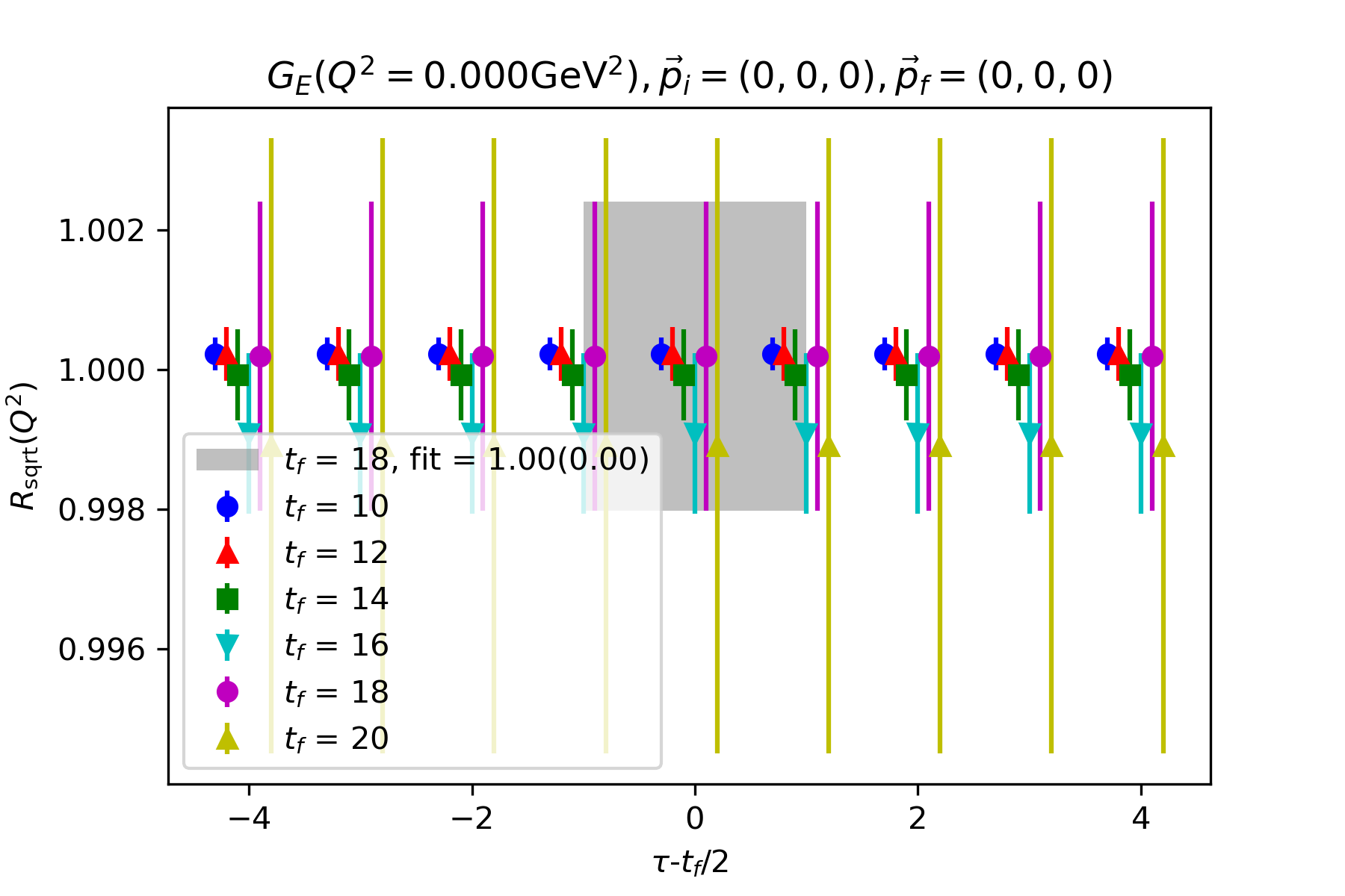
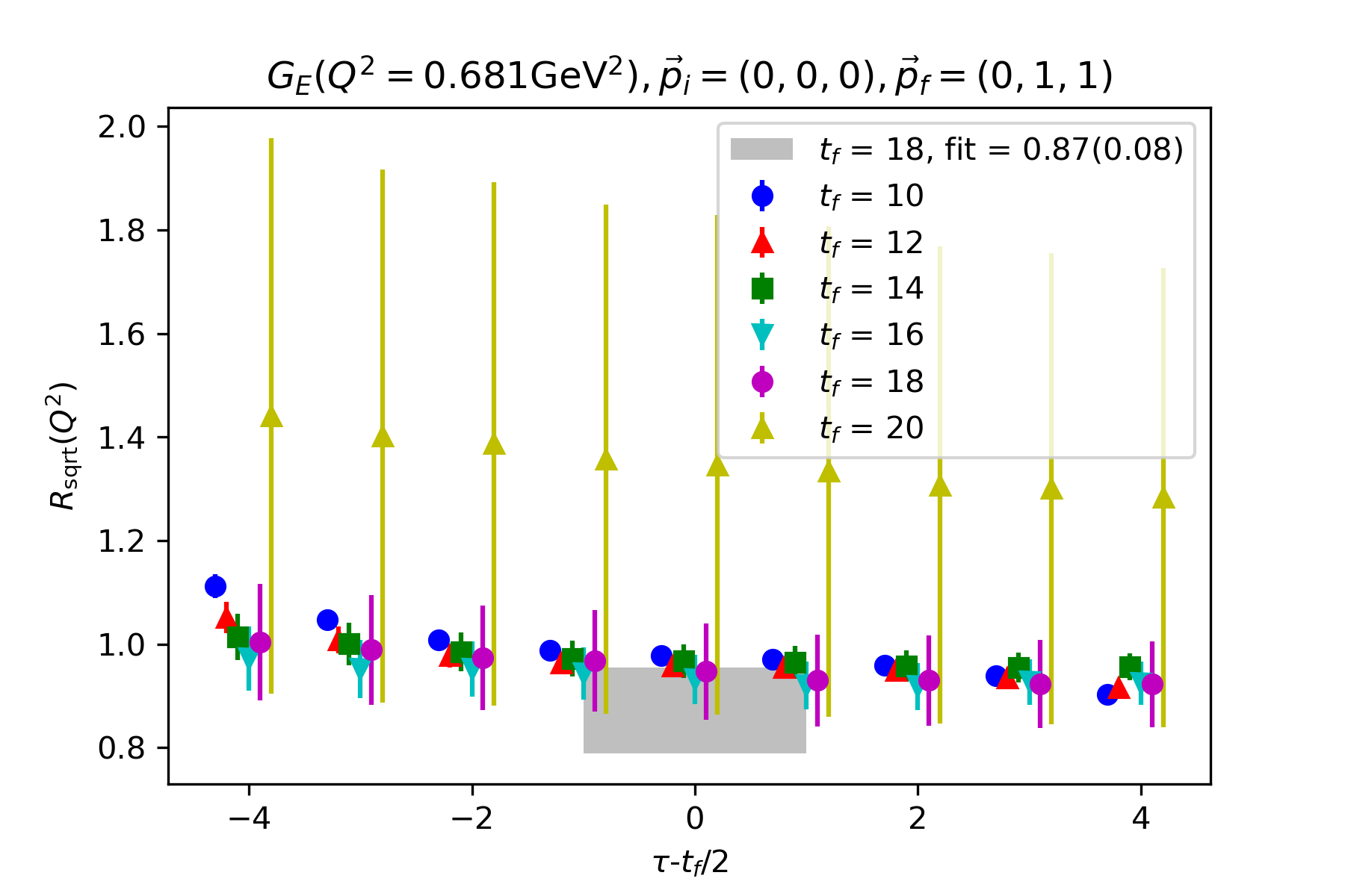
Figure 6: Examples of the $G_{E}$ form factor fitted with constant fit for the up quark at source-sink separation = 18 in the lattice units. The grey bands represent the fitted form factors. The figure in the left and right panels show fit to the down, $d$-quark and up, $u$-quark form factors respectively.

Next, we discuss the determination of the nucleon elastic form factor $G_{E}(Q^{2})$ using the fit described in Sec. V.2 using the hadronic tensor formalism. The $G_{E}(Q^{2})$ form factor can be extracted from the fitted parameter of the spectral weight $W_{1}$ by fitting the matrix element using the fit form (19). All the kinematic factors in Eq. (19) are obtained from the fit parameter $\Delta E_{1}$ for a given $\vec{q}$ and are listed in Table 1. In Fig. 7, we show the determination of the $G_{E}(Q^{2})$ form factor obtained from the hadronic tensor in the range of $Q^{2}\in[0,1.62]$ GeV². Note that, the four-momentum transfers, $Q^{2}$ in the hadronic tensor formalism are obtained from the fitted parameters $\Delta E_{n}$ and that is why they have uncertainty along the $x$-axis in Fig. 7.

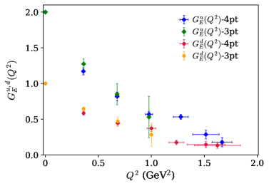
Figure 7: Determination of the nucleon Sachs electric form factor $G_{E}(Q^{2})$ in the range of $Q^{2}\in[0,1.62]$ GeV² using the hadronic tensor formalism. For comparison purposes, $G_{E}(Q^{2})$ form factors obtained from the nucleon 3pt function are also plotted for the first three nonzero momentum transfers including $Q^{2}=0$ GeV². The error bars in the determination of $G_{E}(Q^{2})$ from the 3pt function encompass both statistical and systematic uncertainties, which are added in quadrature.

We present a comparison of $G_{E}(Q^{2})$ determined from the 4pt and 3pt functions in Fig. 7. It is important to note that the $Q^{2}$-values obtained for the nucleon 3pt function calculation derived from the nucleon mass and the three-momentum transfer $\vec{q}$ through the dispersion relation may not necessarily coincide with those obtained in the 4pt functional calculation. However, they are found to be consistent within the uncertainty range of the $Q^{2}$-values obtained through the hadronic tensor formalism. Consequently, for the sake of a schematic comparison in Fig. 7, we align the central values of the $Q^{2}$ from the nucleon 3pt function with those obtained from the hadronic tensor formalism. As mentioned earlier, we have incorporated the differences between the fitting values at $t=18$ and those at $t=14,16$ to estimate the systematic uncertainty in the determination of the $G_{E}$ form factor through the 3pt function calculation. It is worth noting that the fit to the matrix elements at $t=18$ for $Q^{2}=0.68$ and $0.98$ GeV² exhibit larger uncertainties compared to those at $t=14,16$. This can be seen from the $G_{E}^{u}(Q^{2})$ at $Q^{2}=0.68$ GeV², determined from $t=18$ data points as illustrated using the fit band in Fig. 6. Along with these large uncertainties coming from the fit to the matrix elements at $t=18$, the differences from the fits at $t=14,16$ are included in the systematic uncertainties and are reflected as large error bars in the $G_{E}(Q^{2})$ at $Q^{2}=0.68$ and $0.98$ GeV² in Fig. 7. However, as can be seen from the right panel in Fig. 6, the matrix elements at $t=18$ are still statistically consistent with the lattice data points at $t=14,16$ which have much smaller uncertainties. Given that we applied a constant fit to the $t=18$ data points due to our inability to perform a proper excited-state fit to the 3pt functions, as a conservative approach, we present these constant fits at $t=18$ with a larger uncertainty as our final results. The numerical agreement observed in the $G_{E}(Q^{2})$ values between the 3pt and the 4pt extractions affirms the reliability of extracting form factors using the hadronic tensor formalism and our method to extract it using the fit form in Eq. (19).

V.4 Nucleon to its radial excitation transition form factor

In this section, we present the results of the nucleon’s transition to its finite-volume radial excitations from the $W_{2}$ spectral weights, as determined according to Eq. (19). All kinematic factors are determined from the fitted parameters $\Delta E_{n}$. Given that we employed the fit form described in Eq. (19) for fitting the hadronic tensor, our expectation is to determine the properties of both the first and the second finite-volume radial excitations of the nucleon. However, as previously discussed, the current statistics of the lattice data do not allow distinguishing two closely situated states, where the separation might be on the order of approximately $300$ MeV. Consequently, we obtain similar transition form factors associated with states having masses $m_{2}^{*}$ and $m_{3}^{*}$. Aside from not being able to resolve states 2 and 3, in a three-state fit, the highest state result is not reliable because of the contamination from much higher states.

We note that for $\vec{q}=(0,0,1)$ and $(0,1,1)$ the four-momentum transfers $Q^{2}$ determined from $\Delta E_{n}$ are negative. In this work , we shall focus on the cases for the positive momentum transfers in Fig. 8. For comparison, a previous lattice QCD study of the nucleon-to-Roper transition form factors simulated at a pion mass of approximately $720$ MeV can be found in [70].

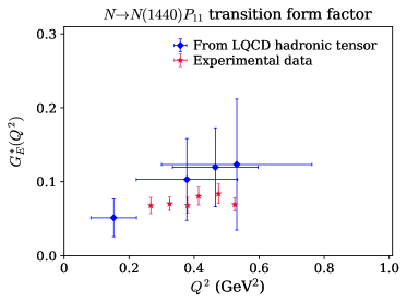
Figure 8: Determination of the nucleon to its finite-volume first radial excitation transition electric form factor in the momentum transfer range of $Q^{2}\in[0.15,0.53]$ GeV². Based on the discussion in the main text, this state is identified with the Roper state in comparison with the experimental data and labeled as the $N\to N(1440)P_{11}$ transition form factor. The experimental data points are extracted from Ref. [71] only in a limited range of $Q^{2}$ for comparison with the lattice QCD calculation within the hadronic tensor formalism.

From Fig. 8, we see that the $G_{E}^{*}(Q^{2})$ form factor tends to go to zero as $Q^{2}\to 0$ as expected from [52, 72]. Although we do not explicitly insert the current in Eq. (8) in the determination of the hadronic tensor, the expected behavior of $G_{E}^{*}(Q^{2})$ clearly demonstrates that the inclusive hadronic tensor allows us to probe the nucleon to its radial excitation transition form factors from a lattice QCD calculation. We compare the lattice QCD determination of $G_{E}^{*}(Q^{2})$ with that extracted from the experimental data [73, 71] and observe good qualitative agreement within (albeit, rather large) uncertainty.

To draw a connection between the lattice QCD determination of the transition form factor and the experimental determination of the relevant quantity, we first discuss how the nucleon to Roper transition form factor is extracted from the experimental data which are plotted in Fig. 8 in a limited $Q^{2}$ range, determined from experimental data in [71]. Through the nucleon electroexcitation reactions, $eN\to e^{\prime}N^{*}$, the excitation of nucleon resonances occurs through the intermediate processes $\gamma^{*}N\to N^{*}$, where $\gamma^{*}$ is a virtual photon, and the cross sections of the processes can usually be expressed in terms of the electromagnetic transition form factors, or helicity amplitudes $S_{1/2}(Q^{2})$ and $A_{1/2}(Q^{2})$. For this calculation, the relevant amplitude is the longitudinal helicity amplitude, $S_{1/2}(Q^{2})$, which measures the resonance response to the longitudinal component of the virtual photon:

$$S_{1/2}(Q^{2})=\sqrt{2\pi\alpha\frac{Q^{2}+(m_{2}^{*}-m_{N})^{2}}{m_{N}(m_{2}^{*2}-m_{N}^{2})}}\frac{m_{2}^{*}+m_{N}}{2\sqrt{2}Q^{2}m_{2}^{*}}\sqrt{[Q^{2}+(m_{2}^{*}-m_{N})^{2}][Q^{2}+(m_{2}^{*}+m_{N})^{2}]}~{}G_{E}^{*}(Q^{2}),$$ (21)

where $\alpha=1/137$ is the fine structure constant. The results on $Q^{2}$-dependence of the $\gamma_{v}pN^{*}$ electrocouplings extracted from the experimental data are not able to provide direct access to the Roper wave function and a model for Roper resonance structure is needed that relates the Roper resonance wave function to the results on $Q^{2}$ evolution of $N(1440)1/2^{+}$ electrocouplings. For these purposes, the continuum Schwinger method (CSM) approach has been used [74, 75] in Ref. [71]. This approach has described successfully, within the common framework, the experimental results of pion and nucleon elastic form factors, and $\gamma_{v}pN^{*}$ electrocouplings of $\Delta(1232)3/2^{+}$, $N(1440)1/2^{+}$, $\Delta(1600)3/2^{+}$ electrocouplings for $Q^{2}<5.0$ GeV². This approach predicts a node in the Roper wave function and gives very good agreement with the results on $N(1440)1/2^{+}$ electrocouplings at $Q^{2}>2.0$ GeV². The range of $Q^{2}>2.0$ GeV² corresponds to the distances where the contribution from 3 dressed/constituent quarks is the biggest in the Fock-space wavefunction (in comparison with meson-baryon cloud contribution) and where CSM predictions can be directly confronted with the results on $\gamma_{v}pN^{*}$ electrocouplings. The fat that a good description of the $Q^{2}$ dependence of the $N(1440)1/2^{+}$ electrocouplings experimental data achieved within the CSM approach [75] can most likely be interpreted as the existence of the node in the $N(1440)1/2^{+}$ wave function.  Moreover, as described in the PDG [64], at high $Q^{2}$, both the helicity amplitudes for $N(1440)1/2^{+}$ are qualitatively described by the light front quark models [76]. In fact, the existence of the radial node of the Roper resonance wavefunction has been observed in the lattice QCD calculations [77, 78, 79, 80], indicating the Roper as a predominantly first radial excitation of the $3q$ ground state. For various interpretations and model calculations on the Roper resonance, see Refs. [21, 73, 81, 82, 83, 84, 85, 86, 87, 88, 89, 90, 19, 91, 92, 93].

At this point, we compare the helicity amplitude, denoted as $S_{1/2}(Q^{2})$ [Eq. (21)], determined from the hadronic tensor formalism with the corresponding values extracted the from experimental data, as depicted in Fig. 9. It is crucial to acknowledge that the presence of $Q^{2}$ in the denominator of $S_{1/2}$ in Eq. (21) results in large uncertainties in the lattice data points, especially when the values of $Q^{2}$ are small in the present calculation. Nonetheless, the data presented in Fig. 9 underscores the significant impact of the lattice QCD calculations in determining the helicity amplitudes at very small $Q^{2}$, particularly near the real photon point where the longitudinal helicity amplitude $S_{1/2}$ is maximal. This contribution from lattice QCD calculations is particularly valuable in complementing the low $Q^{2}\to 0$ region where there are not ample data points available from experiments.

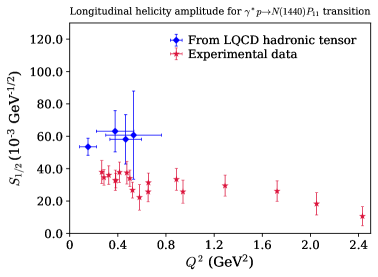
Figure 9: Comparison of the longitudinal helicity amplitude, $S_{1/2}(Q^{2})$ associated with the nucleon to Roper transition form factor. The estimation of the $S_{1/2}$ amplitude in lattice QCD is based on the $G_{E}^{*}(Q^{2})$ form factor, as detailed in the main text. The red data points represent the experimental extraction of $S_{1/2}$, compiled from the reference [71]. As explained in the text, the helicity amplitude depicted in Fig. 9 will progressively approach the experimental determination as the lattice QCD calculation approaches the physical quark mass.

It is expected that the helicity amplitude in Fig. 9 will shift towards the experimental determination as one moves towards the physical quark mass in the lattice QCD calculation. This can be readily understood from the definition of $S_{1/2}$ in Eq. (21). For instance, when considering momentum transfer represented by $\vec{q}=(1,1,1)$, leading to a value of $Q^{2}\approx 0.15$ GeV², the kinematic factor associated with $G_{E}^{*}$ in the equation for $S_{1/2}$ is approximately 25% smaller when calculated using the physical values of nucleon mass, $m_{N}=0.938$ GeV and Roper mass, $m_{2}^{*}=1.440$ GeV, in contrast to kinematic factor obtained from the heavier $m_{N}$ and $m_{2}^{*}$ from the fit to the lattice data as indicated in Table 1. Furthermore, as previously discussed in Sec. V.2, had we employed a two-exponential fit instead of a three-exponential fit on the lattice data, both the $G_{E}^{*}(Q^{2})$ form factor and the corresponding $S_{1/2}(Q^{2})$ would have seen an approximate increase by a factor of $\sqrt{2}$. This effect can be regarded as a systematic uncertainty arising from our inability to differentiate between states 2 and 3 in the context of the three exponential fits.

VI Discussions and conclusions

In this paper, we present the results of a lattice QCD investigation into the determination of the nucleon’s elastic and resonance structure through a single calculation, employing the hadronic tensor formalism. While this study represents a preliminary exploration in this direction, the semi-quantitative agreement observed with the experimental data is both promising and motivating, despite the fact that the lattice is small and the pion mass is not at the physical point. It underscores the prospective utility of the future development of the hadronic tensor formalism in understanding nucleon’s low-lying resonance structures and in offering crucial constraints on the physics involved in modeling many-body nuclear theory, especially in the context of studying neutrino oscillation experiments. In particular, the hadronic tensor formalism includes the inclusive contribution of all the intermediate states which is crucial to providing information for the neutrino scattering experiments at low energies. Furthermore, the utilization of the hadronic tensor formalism extends to the investigation of nucleon deep inelastic structure functions. This feature enhances the comprehensiveness of our approach, enabling the simultaneous examination of the nucleon’s elastic, resonance, and deep inelastic structures within a unified framework.

It is worthwhile pointing out that there are current-induced $N\pi$ states contamination for the nucleon excited states with $q^{3}$ interpolation field [94, 95, 96]. This affects mostly the pseudo-scalar and axial currents. In the present work, we studied the charge current which should not have such a concern. This needs to be investigated in future calculations involving the axial current. The nucleon interpolating operator couples not only to the nucleon itself but also to its excitations and multi-hadron states with the same quantum numbers. Investigations in this direction to improve the interpolating operator coupling to multi-hadron states are essential for properly identifying both the spectrum and the nature of states such as the radial excitations of the nucleon and $P$-wave $N\pi$ states [97, 98, 99, 20, 100]. Moreover, we should mention that the Roper is a resonance which decays into $N\pi,N\pi\pi,\cdots$ and to find its pole mass and width on the lattice, one should perform the scattering phase shift calculation including the $N\pi$ channel using the Lüscher method [101, 102, 103], such as in Ref. [98]. This also requires more theoretical developments [99, 17]. Certainly, these represent crucial avenues for future research in comprehending the impacts of multi-hadron states in the development of nucleon interpolation fields and the investigation of the relevant spectra of the hadronic states.

We also plan to extend this formalism for the determination of the magnetic and the axial structures of the nucleon in the elastic and resonance regions and the deep-inelastic structure functions. In particular, we plan to extend this calculation for testing the feasibility of $N\to\Delta$ transition form factors. At intermediate energies, above $0.5$ GeV, one pion production becomes relevant. The knowledge of the elementary process $\nu+N\to l+N^{\prime}+\pi$ is not so well established. Most of the theoretical models assume the dominance of the $\Delta(1232)$ resonance mechanisms [104, 105, 106, 107, 108]. The major uncertainties of these models appear in the $N\to\Delta$ transition axial form factors that are fitted, with some theoretical ansatz to the available data. While $N\to\Delta$ transition form factor was calculated in lattice QCD [109, 110, 111] about a decade ago, it is desirable to obtain nucleon axial and $N\to\Delta$ transition form factor using the hadronic tensor formalism. As noted in a recent publication [112], the lack of precise knowledge of the $N\to\Delta$ transition form factor results in unconstrained uncertainties in the two-body current contributions to the flux-averaged cross sections. Therefore, a lattice QCD calculation of this transition form factor using the hadronic tensor formalism can provide the theoretical constraints needed for the construction of the two-body current operator.

Finally, while our work represents a significant step forward, we acknowledge its limitations and emphasize the necessity for various systematic improvements in future researches. These enhancements are crucial for directly impacting the nuclear physics programs aimed at studying the resonance structures and advancing the neutrino oscillation experiments. As emphasized above, it is of fundamental importance to comprehensively investigate various sources of systematic uncertainties, including the removal of the potential contamination from the $N\pi$ scattering states to obtain the nucleon state, pion mass, lattice spacing, and finite volume effects, before arriving at robust conclusions. In future studies, we aim to investigate a number of ways that the present calculation can be improved and confidence in estimating the systematic uncertainties involved in the calculation of the hadronic tensor on the lattice can be increased. However, the notable agreement between the lattice data and the experimental results is quite encouraging, particularly for this initial feasibility study aimed at exploring the resonance structure of the nucleon through the hadronic tensor formalism.

VII Acknowledgement

We would like to thank all the members of the $\chi$QCD collaboration for fruitful and stimulating exchanges. We are grateful to A. Rothkoph for letting us use his code for the Bayesian Reconstruction. K.F.L. wishes to thank S. Brodsky H. Meyer and J.W. Qiu for fruitful discussions. R.S.S. acknowledges A. Hanlon, T. Izubuchi, L. Leskovec, A. Meyer, S. Mukherjee, and V. Mokeev for helpful discussions. This work is supported in part by the Office of Science of the U.S. Department of Energy under Grant No. DE-SC0013065 and No. DE-AC05-06OR23177, which is within the framework of the TMD Topical Collaboration. R.S.S. is supported by the Special Postdoctoral Researchers Program of RIKEN and RIKEN-BNL Research Center. The authors also acknowledge partial support by the U.S. Department of Energy, Office of Science, Office of Nuclear Physics under the umbrella of the Quark-Gluon Tomography (QGT) Topical Collaboration with Award DE-SC0023646. This work used Stampede time under the Extreme Science and Engineering Discovery Environment (XSEDE), which is supported by National Science Foundation Grant No. ACI-1053575. We also used resources on Frontera at Texas Advanced Computing Center (TACC). We also thank the National Energy Research Scientific Computing Center (NERSC) for providing HPC resources that have contributed to the research results reported within this paper. We acknowledge the facilities of the USQCD Collaboration used for this research in part, which are funded by the Office of Science of the U.S. Department of Energy.

References

- Liu and Dong [1994] K.-F. Liu and S.-J. Dong, Phys. Rev. Lett. 72, 1790 (1994), arXiv:hep-ph/9306299 .
- Liu [2000] K.-F. Liu, Phys. Rev. D 62, 074501 (2000), arXiv:hep-ph/9910306 .
- Kronfeld et al. [2019] A. S. Kronfeld, D. G. Richards, W. Detmold, R. Gupta, H.-W. Lin, K.-F. Liu, A. S. Meyer, R. Sufian, and S. Syritsyn (USQCD), Eur. Phys. J. A 55, 196 (2019), arXiv:1904.09931 [hep-lat] .
- Ruso et al. [2022] L. A. Ruso et al., (2022), arXiv:2203.09030 [hep-ph] .
- Abi et al. [2020] B. Abi et al. (DUNE), JINST 15, T08008 (2020), arXiv:2002.02967 [physics.ins-det] .
- Abe et al. [2018] K. Abe et al. (Hyper-Kamiokande), (2018), arXiv:1805.04163 [physics.ins-det] .
- Formaggio and Zeller [2012] J. A. Formaggio and G. P. Zeller, Rev. Mod. Phys. 84, 1307 (2012), arXiv:1305.7513 [hep-ex] .
- Alvarez-Ruso et al. [2018] L. Alvarez-Ruso et al. (NuSTEC), Prog. Part. Nucl. Phys. 100, 1 (2018), arXiv:1706.03621 [hep-ph] .
- Sufian et al. [2020a] R. S. Sufian, K.-F. Liu, and D. G. Richards, JHEP 01, 136 (2020a), arXiv:1809.03509 [hep-ph] .
- Sufian et al. [2017a] R. S. Sufian, Y.-B. Yang, A. Alexandru, T. Draper, J. Liang, and K.-F. Liu, Phys. Rev. Lett. 118, 042001 (2017a), arXiv:1606.07075 [hep-ph] .
- Sufian et al. [2017b] R. S. Sufian, Y.-B. Yang, J. Liang, T. Draper, and K.-F. Liu, Phys. Rev. D 96, 114504 (2017b), arXiv:1705.05849 [hep-lat] .
- Sufian [2017] R. S. Sufian, Phys. Rev. D 96, 093007 (2017), arXiv:1611.07031 [hep-ph] .
- Liang et al. [2018a] J. Liang, Y.-B. Yang, T. Draper, M. Gong, and K.-F. Liu, Phys. Rev. D 98, 074505 (2018a), arXiv:1806.08366 [hep-ph] .
- Aguilar-Arevalo et al. [2010] A. A. Aguilar-Arevalo et al. (MiniBooNE), Phys. Rev. D 82, 092005 (2010), arXiv:1007.4730 [hep-ex] .
- Aguilar-Arevalo et al. [2015] A. A. Aguilar-Arevalo et al. (MiniBooNE), Phys. Rev. D 91, 012004 (2015), arXiv:1309.7257 [hep-ex] .
- Liang et al. [2018b] J. Liang, K.-F. Liu, and Y.-B. Yang, EPJ Web Conf. 175, 14014 (2018b), arXiv:1710.11145 [hep-lat] .
- Meyer et al. [2022] A. S. Meyer, A. Walker-Loud, and C. Wilkinson, (2022), 10.1146/annurev-nucl-010622-120608, arXiv:2201.01839 [hep-lat] .
- Burkert [2005] V. D. Burkert, Prog. Part. Nucl. Phys. 55, 108 (2005).
- Aznauryan et al. [2013] I. G. Aznauryan et al., Int. J. Mod. Phys. E 22, 1330015 (2013), arXiv:1212.4891 [nucl-th] .
- Detmold et al. [2019] W. Detmold, R. G. Edwards, J. J. Dudek, M. Engelhardt, H.-W. Lin, S. Meinel, K. Orginos, and P. Shanahan (USQCD), Eur. Phys. J. A 55, 193 (2019), arXiv:1904.09512 [hep-lat] .
- Aznauryan and Burkert [2012a] I. G. Aznauryan and V. D. Burkert, Prog. Part. Nucl. Phys. 67, 1 (2012a), arXiv:1109.1720 [hep-ph] .
- Carlson and Vanderhaeghen [2008] C. E. Carlson and M. Vanderhaeghen, Phys. Rev. Lett. 100, 032004 (2008), arXiv:0710.0835 [hep-ph] .
- Tiator and Vanderhaeghen [2009] L. Tiator and M. Vanderhaeghen, Phys. Lett. B 672, 344 (2009), arXiv:0811.2285 [hep-ph] .
- Braun et al. [2019] V. M. Braun, A. Vladimirov, and J.-H. Zhang, Phys. Rev. D 99, 014013 (2019), arXiv:1810.00048 [hep-ph] .
- Ji [2013] X. Ji, Phys. Rev. Lett. 110, 262002 (2013), arXiv:1305.1539 [hep-ph] .
- Ji [2014] X. Ji, Sci. China Phys. Mech. Astron. 57, 1407 (2014), arXiv:1404.6680 [hep-ph] .
- Chambers et al. [2017] A. J. Chambers, R. Horsley, Y. Nakamura, H. Perlt, P. E. L. Rakow, G. Schierholz, A. Schiller, K. Somfleth, R. D. Young, and J. M. Zanotti, Phys. Rev. Lett. 118, 242001 (2017), arXiv:1703.01153 [hep-lat] .
- Radyushkin [2017] A. V. Radyushkin, Phys. Rev. D 96, 034025 (2017), arXiv:1705.01488 [hep-ph] .
- Ma and Qiu [2018a] Y.-Q. Ma and J.-W. Qiu, Phys. Rev. Lett. 120, 022003 (2018a), arXiv:1709.03018 [hep-ph] .
- Liu [2020] K.-F. Liu, Phys. Rev. D 102, 074502 (2020), arXiv:2007.15075 [hep-ph] .
- Liu et al. [1999] K. F. Liu, S. J. Dong, T. Draper, D. Leinweber, J. H. Sloan, W. Wilcox, and R. M. Woloshyn, Phys. Rev. D 59, 112001 (1999), arXiv:hep-ph/9806491 .
- Gottfried [1967] K. Gottfried, Phys. Rev. Lett. 18, 1174 (1967).
- Hou et al. [2022] T.-J. Hou, M. Yan, J. Liang, K.-F. Liu, and C. P. Yuan, Phys. Rev. D 106, 096008 (2022), arXiv:2206.02431 [hep-ph] .
- Batelaan et al. [2023] M. Batelaan et al. (QCDSF/UKQCD/CSSM, CSSM, UKQCD, QCDSF), Phys. Rev. D 107, 054503 (2023), arXiv:2209.04141 [hep-lat] .
- Liang and Liu [2020] J. Liang and K.-F. Liu (QCD), PoS LATTICE2019, 046 (2020), arXiv:2008.12389 [hep-lat] .
- Constantinou and Panagopoulos [2017] M. Constantinou and H. Panagopoulos, Phys. Rev. D 96, 054506 (2017), arXiv:1705.11193 [hep-lat] .
- Chen et al. [2018] J.-W. Chen, T. Ishikawa, L. Jin, H.-W. Lin, Y.-B. Yang, J.-H. Zhang, and Y. Zhao, Phys. Rev. D 97, 014505 (2018), arXiv:1706.01295 [hep-lat] .
- Ji et al. [2021a] X. Ji, Y. Liu, A. Schäfer, W. Wang, Y.-B. Yang, J.-H. Zhang, and Y. Zhao, Nucl. Phys. B 964, 115311 (2021a), arXiv:2008.03886 [hep-ph] .
- Huo et al. [2021] Y.-K. Huo et al. (Lattice Parton Collaboration (LPC)), Nucl. Phys. B 969, 115443 (2021), arXiv:2103.02965 [hep-lat] .
- Detmold and Lin [2006] W. Detmold and C. J. D. Lin, Phys. Rev. D 73, 014501 (2006), arXiv:hep-lat/0507007 .
- Braun and Müller [2008] V. Braun and D. Müller, Eur. Phys. J. C 55, 349 (2008), arXiv:0709.1348 [hep-ph] .
- Ma and Qiu [2018b] Y.-Q. Ma and J.-W. Qiu, Phys. Rev. D 98, 074021 (2018b), arXiv:1404.6860 [hep-ph] .
- Bali et al. [2018] G. S. Bali, V. M. Braun, B. Gläßle, M. Göckeler, M. Gruber, F. Hutzler, P. Korcyl, A. Schäfer, P. Wein, and J.-H. Zhang, Phys. Rev. D 98, 094507 (2018), arXiv:1807.06671 [hep-lat] .
- Sufian et al. [2019] R. S. Sufian, J. Karpie, C. Egerer, K. Orginos, J.-W. Qiu, and D. G. Richards, Phys. Rev. D 99, 074507 (2019), arXiv:1901.03921 [hep-lat] .
- Sufian et al. [2020b] R. S. Sufian, C. Egerer, J. Karpie, R. G. Edwards, B. Joó, Y.-Q. Ma, K. Orginos, J.-W. Qiu, and D. G. Richards, Phys. Rev. D 102, 054508 (2020b), arXiv:2001.04960 [hep-lat] .
- Can et al. [2020] K. U. Can et al., Phys. Rev. D 102, 114505 (2020), arXiv:2007.01523 [hep-lat] .
- Cichy and Constantinou [2019] K. Cichy and M. Constantinou, Adv. High Energy Phys. 2019, 3036904 (2019), arXiv:1811.07248 [hep-lat] .
- Constantinou et al. [2021] M. Constantinou et al., Prog. Part. Nucl. Phys. 121, 103908 (2021), arXiv:2006.08636 [hep-ph] .
- Ji et al. [2021b] X. Ji, Y.-S. Liu, Y. Liu, J.-H. Zhang, and Y. Zhao, Rev. Mod. Phys. 93, 035005 (2021b), arXiv:2004.03543 [hep-ph] .
- Constantinou et al. [2022] M. Constantinou et al., (2022), arXiv:2202.07193 [hep-lat] .
- Liu [2016] K.-F. Liu, PoS LATTICE2015, 115 (2016), arXiv:1603.07352 [hep-ph] .
- Weber [1990] H. J. Weber, Phys. Rev. C 41, 2783 (1990).
- Aznauryan et al. [2008] I. G. Aznauryan, V. D. Burkert, and T. S. H. Lee, (2008), arXiv:0810.0997 [nucl-th] .
- Liang et al. [2020] J. Liang, T. Draper, K.-F. Liu, A. Rothkopf, and Y.-B. Yang (XQCD), Phys. Rev. D 101, 114503 (2020), arXiv:1906.05312 [hep-ph] .
- Blum et al. [2016] T. Blum et al. (RBC, UKQCD), Phys. Rev. D 93, 074505 (2016), arXiv:1411.7017 [hep-lat] .
- Lee et al. [2023] C. Lee, T. Draper, J. Hua, J. Liang, K.-F. Liu, J. Shi, N. Wang, and Y.-b. Yang, (2023), arXiv:2310.02179 [hep-lat] .
- Burnier and Rothkopf [2013] Y. Burnier and A. Rothkopf, Phys. Rev. Lett. 111, 182003 (2013), arXiv:1307.6106 [hep-lat] .
- Backus and Gilbert [1970] G. Backus and F. Gilbert, Philosophical Transactions of the Royal Society of London A: Mathematical, Physical and Engineering Sciences 266 (1970), doi.org/10.1098/rsta.1970.0005.
- Hansen et al. [2017] M. T. Hansen, H. B. Meyer, and D. Robaina, Phys. Rev. D 96, 094513 (2017), arXiv:1704.08993 [hep-lat] .
- Asakawa et al. [2001] M. Asakawa, T. Hatsuda, and Y. Nakahara, Prog. Part. Nucl. Phys. 46, 459 (2001), arXiv:hep-lat/0011040 .
- Bailas et al. [2020] G. Bailas, S. Hashimoto, and T. Ishikawa, PTEP 2020, 043B07 (2020), arXiv:2001.11779 [hep-lat] .
- Alexandrou et al. [2023] C. Alexandrou et al. (Extended Twisted Mass Collaboration (ETMC)), Phys. Rev. Lett. 130, 241901 (2023), arXiv:2212.08467 [hep-lat] .
- Rothkopf [2022] A. Rothkopf, Front. Phys. 10, 1028995 (2022), arXiv:2208.13590 [hep-lat] .
- Workman et al. [2022] R. L. Workman et al. (Particle Data Group), PTEP 2022, 083C01 (2022).
- Alexandrou et al. [2018] C. Alexandrou, M. Constantinou, K. Hadjiyiannakou, K. Jansen, C. Kallidonis, G. Koutsou, and A. Vaquero Avilés-Casco, Phys. Rev. D 97, 094504 (2018), arXiv:1801.09581 [hep-lat] .
- Alexandrou et al. [2019] C. Alexandrou, S. Bacchio, M. Constantinou, J. Finkenrath, K. Hadjiyiannakou, K. Jansen, G. Koutsou, and A. Vaquero Aviles-Casco, Phys. Rev. D 100, 014509 (2019), arXiv:1812.10311 [hep-lat] .
- Djukanovic et al. [2023] D. Djukanovic, G. von Hippel, H. B. Meyer, K. Ottnad, M. Salg, and H. Wittig, (2023), arXiv:2309.06590 [hep-lat] .
- Wang et al. [2021] G. Wang, J. Liang, T. Draper, K.-F. Liu, and Y.-B. Yang (chiQCD), Phys. Rev. D 104, 074502 (2021), arXiv:2006.05431 [hep-ph] .
- Park et al. [2022] S. Park, R. Gupta, B. Yoon, S. Mondal, T. Bhattacharya, Y.-C. Jang, B. Joó, and F. Winter (Nucleon Matrix Elements (NME)), Phys. Rev. D 105, 054505 (2022), arXiv:2103.05599 [hep-lat] .
- Lin et al. [2008] H.-W. Lin, S. D. Cohen, R. G. Edwards, and D. G. Richards, Phys. Rev. D 78, 114508 (2008), arXiv:0803.3020 [hep-lat] .
- Mokeev et al. [2023] V. I. Mokeev, P. Achenbach, V. D. Burkert, D. S. Carman, R. W. Gothe, A. N. Hiller Blin, E. L. Isupov, K. Joo, K. Neupane, and A. Trivedi, Phys. Rev. C 108, 025204 (2023), arXiv:2306.13777 [nucl-ex] .
- Wilson et al. [2012] D. J. Wilson, I. C. Cloet, L. Chang, and C. D. Roberts, Phys. Rev. C 85, 025205 (2012), arXiv:1112.2212 [nucl-th] .
- Burkert and Roberts [2019] V. D. Burkert and C. D. Roberts, Rev. Mod. Phys. 91, 011003 (2019), arXiv:1710.02549 [nucl-ex] .
- Segovia et al. [2015] J. Segovia, B. El-Bennich, E. Rojas, I. C. Cloet, C. D. Roberts, S.-S. Xu, and H.-S. Zong, Phys. Rev. Lett. 115, 171801 (2015), arXiv:1504.04386 [nucl-th] .
- Isupov et al. [2017] E. L. Isupov et al. (CLAS), Phys. Rev. C 96, 025209 (2017), arXiv:1705.01901 [nucl-ex] .
- Aznauryan [2003] I. G. Aznauryan, Phys. Rev. C 67, 015209 (2003), arXiv:nucl-th/0206033 .
- Chen [2007] Y. Chen, Mod. Phys. Lett. A 22, 583 (2007).
- Roberts et al. [2013] D. S. Roberts, W. Kamleh, and D. B. Leinweber, Phys. Lett. B 725, 164 (2013), arXiv:1304.0325 [hep-lat] .
- Roberts et al. [2014] D. S. Roberts, W. Kamleh, and D. B. Leinweber, Phys. Rev. D 89, 074501 (2014), arXiv:1311.6626 [hep-lat] .
- Sun et al. [2020] M. Sun et al. (xQCD), Phys. Rev. D 101, 054511 (2020), arXiv:1911.02635 [hep-ph] .
- Mai et al. [2022] M. Mai, M. Döring, C. Granados, H. Haberzettl, J. Hergenrather, U.-G. Meißner, D. Rönchen, I. Strakovsky, and R. Workman (Jülich-Bonn-Washington), Phys. Rev. C 106, 015201 (2022), arXiv:2111.04774 [nucl-th] .
- Suzuki et al. [2010] N. Suzuki, T. Sato, and T. S. H. Lee, Phys. Rev. C 82, 045206 (2010), arXiv:1006.2196 [nucl-th] .
- Mokeev and Carman [2022] V. I. Mokeev and D. S. Carman (CLAS), Few Body Syst. 63, 59 (2022), arXiv:2202.04180 [nucl-ex] .
- Brodsky et al. [2020] S. J. Brodsky et al., Int. J. Mod. Phys. E 29, 2030006 (2020), arXiv:2006.06802 [hep-ph] .
- Kamano [2018] H. Kamano, Few Body Syst. 59, 24 (2018).
- Barabanov et al. [2021] M. Y. Barabanov et al., Prog. Part. Nucl. Phys. 116, 103835 (2021), arXiv:2008.07630 [hep-ph] .
- Cano and Gonzalez [1998] F. Cano and P. Gonzalez, Phys. Lett. B 431, 270 (1998), arXiv:nucl-th/9804071 .
- Giannini and Santopinto [2015] M. M. Giannini and E. Santopinto, Chin. J. Phys. 53, 020301 (2015), arXiv:1501.03722 [nucl-th] .
- Capstick and Roberts [2000] S. Capstick and W. Roberts, Prog. Part. Nucl. Phys. 45, S241 (2000), arXiv:nucl-th/0008028 .
- Obukhovsky et al. [2019] I. T. Obukhovsky, A. Faessler, D. K. Fedorov, T. Gutsche, and V. E. Lyubovitskij, Phys. Rev. D 100, 094013 (2019), arXiv:1909.13787 [hep-ph] .
- Aznauryan and Burkert [2012b] I. G. Aznauryan and V. D. Burkert, Phys. Rev. C 85, 055202 (2012b), arXiv:1201.5759 [hep-ph] .
- de Teramond and Brodsky [2012] G. F. de Teramond and S. J. Brodsky, AIP Conf. Proc. 1432, 168 (2012), arXiv:1108.0965 [hep-ph] .
- Ramalho and Peña [2023] G. Ramalho and M. T. Peña, (2023), arXiv:2306.13900 [hep-ph] .
- Bar [2019a] O. Bar, Phys. Rev. D 99, 054506 (2019a), arXiv:1812.09191 [hep-lat] .
- Bar [2019b] O. Bar, Phys. Rev. D 100, 054507 (2019b), arXiv:1906.03652 [hep-lat] .
- Jang et al. [2020] Y.-C. Jang, R. Gupta, B. Yoon, and T. Bhattacharya, Phys. Rev. Lett. 124, 072002 (2020), arXiv:1905.06470 [hep-lat] .
- Lang and Verduci [2013] C. B. Lang and V. Verduci, Phys. Rev. D 87, 054502 (2013), arXiv:1212.5055 [hep-lat] .
- Lang et al. [2017] C. B. Lang, L. Leskovec, M. Padmanath, and S. Prelovsek, Phys. Rev. D 95, 014510 (2017), arXiv:1610.01422 [hep-lat] .
- Briceno et al. [2018] R. A. Briceno, J. J. Dudek, and R. D. Young, Rev. Mod. Phys. 90, 025001 (2018), arXiv:1706.06223 [hep-lat] .
- Mai et al. [2023] M. Mai, U.-G. Meißner, and C. Urbach, Phys. Rept. 1001, 1 (2023), arXiv:2206.01477 [hep-ph] .
- Luscher [1986a] M. Luscher, Commun. Math. Phys. 104, 177 (1986a).
- Luscher [1986b] M. Luscher, Commun. Math. Phys. 105, 153 (1986b).
- Luscher and Wolff [1990] M. Luscher and U. Wolff, Nucl. Phys. B 339, 222 (1990).
- Adler [1968] S. L. Adler, Annals Phys. 50, 189 (1968).
- Schreiner and Von Hippel [1973] P. A. Schreiner and F. Von Hippel, Phys. Rev. Lett. 30, 339 (1973).
- Alvarez-Ruso et al. [1998] L. Alvarez-Ruso, S. K. Singh, and M. J. Vicente Vacas, Phys. Rev. C 57, 2693 (1998), arXiv:nucl-th/9712058 .
- Paschos et al. [2004] E. A. Paschos, J.-Y. Yu, and M. Sakuda, Phys. Rev. D 69, 014013 (2004), arXiv:hep-ph/0308130 .
- Lalakulich and Paschos [2005] O. Lalakulich and E. A. Paschos, Phys. Rev. D 71, 074003 (2005), arXiv:hep-ph/0501109 .
- Alexandrou et al. [2011] C. Alexandrou, G. Koutsou, J. W. Negele, Y. Proestos, and A. Tsapalis, Phys. Rev. D 83, 014501 (2011), arXiv:1011.3233 [hep-lat] .
- Alexandrou et al. [2013a] C. Alexandrou, E. B. Gregory, T. Korzec, G. Koutsou, J. W. Negele, T. Sato, and A. Tsapalis, Phys. Rev. D 87, 114513 (2013a), arXiv:1304.4614 [hep-lat] .
- Alexandrou et al. [2013b] C. Alexandrou, J. W. Negele, M. Petschlies, A. Strelchenko, and A. Tsapalis, Phys. Rev. D 88, 031501 (2013b), arXiv:1305.6081 [hep-lat] .
- Simons et al. [2022] D. Simons, N. Steinberg, A. Lovato, Y. Meurice, N. Rocco, and M. Wagman, (2022), arXiv:2210.02455 [hep-ph] .