Tunable photon-photon correlations in waveguide QED systems with giant atoms

Abstract

We investigate the scattering processes of two photons in a one-dimensional (1D) waveguide coupled to two giant atoms. By adjusting the accumulated phase shifts between the coupling points, we are able to effectively manipulate the characteristics of these scattering photons. Utilizing the Lippmann-Schwinger (LS) formalism, we derive analytical expressions for the wavefunctions describing two photon interacting in separate, braided and nested configurations. Based on these wavefunctions, we also obtian analytical expressions for the incoherent power spectra and second-order correlation functions. In contrast to small atoms, the incoherent spectrum, which is defined by the correlation of the bound state, can exhibit four distinct peaks and a wider frequency range. Additionally, the second order correlation functions in the transmission and reflection fields could be tuned to exhibit either bunching or antibunching upon resonant driving, a behavior that is not possible with small atoms. These unique features offered by the giant atoms in waveguide QED could benefit the generation of non-classical itinerant photons in quantum networks.

I Introduction

Waveguide quantum electrodynamics (QED) have garnered significant interest due to the emergence of unique physical phenomena when atom-photon coupling to a continuum of modes limited to a single dimension [1, 2], as well as for their applications in quantum networks [3, 4, 5, 6]. With advancements in technology, strong coupling has been realized between atomic degrees of freedom (including natural and artificial atoms) and propagating photonic modes within waveguide QED[7, 8]. Strong coupling is characterized by a large Purcell factor, where energy dissipation from the atom into the waveguide surpasses that into modes other than the waveguide [9]. By entering the strong coupling regime, qubits can function as high-quality quantum emitters, enabling demonstration of primitives of quantum networks [10, 11]. Furthermore, there has been a shift towards investigating multi-qubit phenomena in waveguide QED, such as correlated dissipation, waveguide-mediated interactions between multiple qubits, and many-body phenomena [12, 13, 14, 15]. Another interesting effect in waveguide QED is related to photonic modes. The optical nonlinearity becomes apparent on the scale of a few photons, allowing for observation of quantum nonlinear phenomena through optical correlation functions [16, 17, 18, 19, 20, 21]. One manifestation of the nonlinearity is the presence of two- and higher-order photon bound states [22, 9]. In these bound states, photons exhibit strongly correlations, meaning that once one photon is detected, the arrival of another photon is much more likely compared to a random time. It is important to note that photon bound states are distinct from bunched photon states. Photon bound states are quasiparticles with their own dispersion and are eigenstates of the underlying Hamiltonian that describes the nonlinear medium.

In recent years, a new paradigm in quantum optics has emerged, beyond the dipole approximation in the light-atom interaction. This paradigm challenges the assumption that the size of atoms is significantly smaller than the wavelength of the interaction light, giving rise to the concept of “giant atoms”. Giant atoms can couple to light or other bosonic fields at multiple points, which may be spaced wavelengths apart. Such systems can be implemented both with superconducting qubits coupled either to microwave transmission lines [23] or surface acoustic waves [24]. The study of giant atom can be divided into two categories: Markovian and non-Markovian regimes. In the Markovian case, the propagation time for radiation across the atom is much shorter than the rate of interaction with the atom. Multiple coupling points in giant atoms give rise to interference effects, allowing for a coherent exchange interaction between atoms mediated by a waveguide. This can result in effects such as frequency-dependent couplings, Lamb shifts, and relaxation rates [25, 26]. On the other hand, giant atoms in the non-Markovian regime interact with the radiation field at a rate much faster than the time it takes for radiation to propagate across the atom, results in effects such as nonexponential decay [27, 28, 29, 30] and oscillating bound states [31]. Extending the concept of multiple qubits to multiple giant atoms enables the exploration of a diverse and rich range of phenomena. These include waveguide-mediated decoherence-free subspaces [32, 33] and the enhanced spontaneous sudden birth of entanglement [34]. The simplest configuration for studying these phenonmena involves two giant atoms interacting to a waveguide with two coupling points. These layouts can be catagorized into three distinct configurations based on the arrangement of the coupling points: separate, braided, and nested [32]. While most studies have focused on the atomic degrees of freedom [35, 36, 34, 32, 33], there have been some investigations into the photonic degrees of freedom. However, these studies primarily explore the single-excitation subspace [37, 38, 39]. To the best of our knowledge, the optical nonlinearity involving two or multiple photons in giant atoms is less investigated.

The phenomenon of a single two-level atom not being able to emit two photons simultaneously is widely known. This limitation arises due to the fact that the atom can absorb only one photon at a time, resulting in $g^{(2)}(0)=0$ in the reflection channel [40, 41]. By introducing multiple atoms, the constraint can be overcome, and it become possible to manipulate the correlation between photons [42]. This occurs because when one photon becomes trapped within the first atom, there is a probability that the second photon will propagate to and reflect off the subsequent atom. This process leads to the simulated emission of the first photon, effectively allowing the simultaneous emission of two photons. Therefore, the probability of two photons being emitted together is not completely prohibited. A similar scenario unfolds with two giant atoms, exhibiting even more pronounced effects. In this work, we employ the Lippmann-Schwinger (LS) formalism [43, 44, 45] to analyze the two-photon scattering processes involving two giant atoms coupled to a one-dimensional (1D) waveguide, which contains separate, braided, and nested configurations. By utilizing this approach, we are able to obtain the analytical two-photon interacting scattering wavefunctions for these systems. Additionally, the incoherent power spectrum is derived from the correlation of the bound state, with its total flux serving as an indicator of photon-photon correlation. The second-order correlation function provides a direct measure of photon-photon correlation. Through our analysis, we find that the accumulated phase shifts can be utilized to manipulate the photon-photon correlation and the evolution of the second-order correlation for photons scattered by the giant atoms.

The paper is organized as follows. In Sec. II, we present the physical model that describes the waveguide QED system with two giant atoms. Sections III and IV derive the single photon scattering eigenstates and two-photon interacting eigenstates in the three configurations. Sections V and VI analyze the incoherent power spectra and the second-order correlation functions. The conclusions drawn from our study are given in Sec. VII.

II Physical model

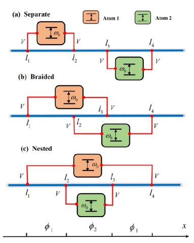
Figure 1: Schematic illustration of two two-level giant atoms with a one-dimensional (1D) waveguide in three distinct configurations: (a) separate, (b) braided, (c) nested. The coupling between the atomic transitions and the waveguide modes occurs at four specific points denoted as $l_{k}$, where $k=1,2,3,4$. The strength of the coupling is represented by $V$. Additionally, the phase shifts acquired between neighboring points are represented by $\phi_{1}$ and $\phi_{2}$.

We consider a waveguide QED system composed of two two-level giant atoms coupled to an open 1D waveguide. Each giant atom only interacts with the waveguide at two specific points, allowing for three distinct configurations: separate, braided, and nested, as illustrated in Fig. 1. The Hamiltonian describing the system in real space is given by ($\hbar=1$ hereafter):

$$\hat{H}^{c}= \left(\omega_{0}-i\frac{\gamma_{e}}{2}\right)\sum_{j=1}^{2}\hat{\sigma}^{+}_{j}\hat{\sigma}^{-}_{j}$$

$$-iv_{g}\int dx\left[\hat{a}_{R}^{\dagger}(x)\partial_{x}\hat{a}_{R}(x)-\hat{a}_{L}^{\dagger}(x)\partial_{x}\hat{a}_{L}(x)\right]$$

$$+\sum_{\alpha=R,L}\sum_{j=1}^{2}V\int dxQ_{j}^{c}(x)\left[\hat{a}_{\alpha}^{\dagger}(x)\hat{\sigma}_{j}^{-}+\hat{a}_{\alpha}(x)\hat{\sigma}_{j}^{+}\right],$$ (1)

where $c=s,b,n$ denotes the separate, braided and nested configurations, respectively. Here the two giant atoms are assumed to be identical with the same transition frequency $\omega_{0}$ and dissipation rate $\gamma_{e}$. The excited and ground states of the $j$th giant atom are represented by $\left|{e}\right\rangle_{j}$ and $\left|{g}\right\rangle_{j}$, respectively. The atomic raising and lowering operators are denoted as $\hat{\sigma}_{j}^{+}=\left|{e}\right\rangle_{jj}\left\langle{g}\right|$ and $\hat{\sigma}_{j}^{-}=\left|{g}\right\rangle_{jj}\left\langle{e}\right|$, respectively. Additionally, $\hat{a}_{R}(x)$ and $\hat{a}_{L}(x)$ correspond to the annihilation operators of right-moving and left-moving photons in the waveguide, and $\nu_{g}$ is the group velocity. For simplicity, we set $\nu_{g}=1$ in the following. The coupling between the giant atoms and the waveguide occurs at specific points identified by $Q_{j}^{c}(x)$, with a common coupling strength $V$. In the case of separate configuration, $Q_{1}^{s}(x)=\delta(x-l_{1})+\delta(x-l_{2})$ refers to the coupling points $l_{1}$ and $l_{2}$ of the first giant atom, while $Q_{2}^{s}(x)=\delta(x-l_{3})+\delta(x-l_{4})$ refers to the coupling points $l_{3}$ and $l_{4}$ of the second giant atom. Similarly, for the braided configuration, $Q_{1}^{b}(x)=\delta(x-l_{1})+\delta(x-l_{3})$, and $Q_{2}^{b}(x)=\delta(x-l_{2})+\delta(x-l_{4})$. In the nested configuration, $Q_{1}^{n}(x)=\delta(x-l_{1})+\delta(x-l_{4})$ and $Q_{2}^{n}(x)=\delta(x-l_{2})+\delta(x-l_{3})$. To exploit the benefits of parity symmetry, the positions of the atoms can be deliberately selected to exhibit symmetry with respect to the origin, i.e. $l_{1}=-l_{4}$ and $l_{2}=-l_{3}$. The phase shifts acquired between neighboring coupling points are given by $\phi_{1}=k(l_{2}-l_{1})=k(l_{4}-l_{3})$ and $\phi_{2}=k(l_{3}-l_{2})$.

The total excitation number of the system is conserved in the interaction, and thus in the single-excitation subspace the eigenstate is

$$|\Phi_{1}^{c}(k)\rangle_{\alpha}= \Bigg{\{}\int dx\left[{\phi_{R}^{\alpha}}(k,x)\hat{a}^{\dagger}_{R}(x)+{\phi_{L}^{\alpha}}(k,x)\hat{a}_{L}(x)\right]$$

$$+\sum_{j=1}^{2}e_{j\alpha}^{c}(k)\hat{\sigma}_{j}^{\dagger}\Bigg{\}}|0\rangle,$$ (2)

where $\alpha$ refers to the direction of incoming photons, and $\phi_{R/L}^{\alpha}(k,x)$ denote the probability amplitudes of creating the right-moving and left-moving photons in real space for the $\alpha$-direction incident photon with wavevector $k$, respectively. Furthermore, $e_{j\alpha}^{c}(k)$ is the excitation amplitude of the $j$th atom in the $c$-configuration, and $\left|{0}\right\rangle$ represents the vacuum state of the system. The probability amplitudes are determined by the Schrödinger equation $\hat{H}^{c}|\Phi_{1}^{c}(k)\rangle_{\alpha}=k|\Phi_{1}^{c}(k)\rangle_{\alpha}$, which fulfill

$$\left(\omega_{0}-i\frac{\gamma_{e}}{2}-k\right)e_{1\alpha}^{c}(k)+V\sum_{\alpha^{\prime}}\int dxQ_{1}^{c}(x)\phi_{\alpha^{\prime}}^{\alpha}(k,x)=0,$$

$$\left(\omega_{0}-i\frac{\gamma_{e}}{2}-k\right)e_{2\alpha}^{c}(k)+V\sum_{\alpha^{\prime}}\int dxQ_{2}^{c}(x)\phi_{\alpha^{\prime}}^{\alpha}(k,x)=0,$$

$$\left(-i\partial_{x}-k\right)\phi_{R}^{\alpha}(k,x)+V\sum_{j=1}^{2}Q_{j}^{c}(x)e_{j\alpha}^{c}(k)=0,$$

$$\left(i\partial_{x}-k\right)\phi_{L}^{\alpha}(k,x)+V\sum_{j=1}^{2}Q_{j}^{c}(x)e_{j\alpha}^{c}(k)=0.$$ (3)

The solutions of three different configurations will be presented explicitly in the following.

III Single-photon scattering eigenstates

In this section, we present the eigenstates of single-photon scattering for each of the three coupling configurations. These eigenstates contain the amplitudes of atomic excitation, as well as the amplitudes for single-photon transmission and reflection.

III.1 Separate-coupling case

In the separate configuration depicted in Fig. 1(a), when a photon is injected in the right-moving direction (i.e., $\alpha=R$) with wavevector $k$, the amplitudes can be concretely expressed in the form

$$\phi_{R}^{R}(k,x)= \frac{e^{ikx}}{\sqrt{2\pi}}\Bigg{[}\theta(l_{1}-x)+\sum_{i=1}^{3}t_{i}^{s}(k)\theta(x-l_{i})\theta(l_{i+1}-x)$$

$$+t_{4}^{s}(k)\theta(x-l_{4})\Bigg{]},$$

$$\phi_{L}^{R}(k,x)= \frac{e^{-ikx}}{\sqrt{2\pi}}\Bigg{[}r_{1}^{s}(k)\theta(l_{1}-x)$$

$$+\sum_{i=2}^{4}r_{i}^{s}(k)\theta(x-l_{i-1})\theta(l_{i}-x)\Bigg{]}.$$ (4)

Within the symmetric topology, by substituting these coefficients into Eqs. (3), we can derive the solutions for transmission and reflection amplitudes as well as atomic excitation amplitudes as follows

$$t_{4}^{s}(k)= (k-\omega_{0}-\Gamma\sin\phi_{1})^{2}/D^{s},$$

$$r_{1}^{s}(k)= -4i\Gamma\cos^{2}\frac{\phi_{1}}{2}\big{\{}(k-\omega_{0})\cos(\phi_{1}+\phi_{2})$$

$$+\Gamma[\sin\phi_{2}+\sin(\phi_{1}+\phi_{2})]\big{\}}/D^{s},$$

$$e_{1R}^{s}(k)= \frac{e^{-i\phi_{2}/2}}{2}\sqrt{\frac{\Gamma}{\pi}}(1+e^{-i\phi_{1}})\Big{\{}k-\omega_{0}+i\Gamma(1+e^{i\phi_{1}})$$

$$-i\frac{\tilde{\Gamma}_{s}}{2}e^{i(\phi_{1}+\phi_{2})}\Big{\}}/D^{s},$$

$$e_{2R}^{s}(k)= \frac{e^{i\phi_{2}/2}}{2}\sqrt{\frac{\Gamma}{\pi}}(1+e^{i\phi_{1}})(k-\omega_{0}-\Gamma\sin\phi_{1})/D^{s},$$

$$D^{s}= \left[\omega_{0}-k-i\Gamma(1+e^{i\phi_{1}})\right]^{2}+\frac{{{\tilde{\Gamma}_{s}}^{2}}}{4},$$ (5)

where $\Gamma=2V^{2}$ represents the decay rate of atomic dissipation to the waveguide continuum, and $\tilde{\Gamma}_{s}=\Gamma e^{i\phi_{2}}(1+e^{i\phi_{1}})^{2}$. In the strong coupling regime [46], the spontaneous decay rate to the waveguide dominates over the decay to other modes, which implies that the Purcell factor is significantly larger, i.e., $\Gamma\gg\gamma_{e}$. Consequently, $\gamma_{e}$ can been ignored in the following discussions.

According to the parity symmetry, for a photon injected in the left-moving direction (i.e., $\alpha=L$), the transmission and reflection amplitudes are equivalent to those of the right-moving case. In addition, the atomic excitation amplitudes also follow this symmetry, which fulfill

$$e_{2L}^{s}(k)=e_{1R}^{s}(k),\hskip 5.0pte_{1L}^{s}(k)=e_{2R}^{s}(k).$$ (6)

III.2 Braided-coupling case

Next, let us consider the braided-coupling case, as shown in Fig. 1(b). In this configuration, the coupling points are given by $Q_{j}^{b}(x)$. Following the same procedure employed in the separate-coupling case, one can determine the corresponding transmission and reflection amplitudes, as well as the atomic excitation amplitudes, which are

$$t_{4}^{b}(k)= \big{[}(k-\omega_{0})^{2}-2\Gamma(k-\omega_{0})\sin(\phi_{1}+\phi_{2})$$

$$+\Gamma^{2}\sin\phi_{1}(\sin\phi_{1}-2\sin\phi_{2})\big{]}/D^{b},$$

$$r_{1}^{b}(k)= -4i\Gamma\cos^{2}\frac{\phi_{1}+\phi_{2}}{2}\big{[}(k-\omega_{0})\cos\phi_{1}$$

$$+\Gamma\sin\phi_{1}\big{]}/D^{b},$$

$$e_{1R}^{b}(k)= \frac{e^{i\phi_{2}/2}}{2}\sqrt{\frac{\Gamma}{\pi}}\left[1+e^{-i(\phi_{1}+\phi_{2})}\right]\Big{[}k-\omega_{0}$$

$$-i\frac{\Gamma}{2}\left(-1+e^{i2\phi_{1}}\right)\left(2+e^{i(\phi_{1}+\phi_{2})}\right)\Big{]}/D^{b},$$

$$e_{2R}^{b}(k)= \frac{e^{i\phi_{2}/2}}{2}\sqrt{\frac{\Gamma}{\pi}}\left[1+e^{-i(\phi_{1}+\phi_{2})}\right]\Big{[}e^{i\phi_{1}}(k-\omega_{0})$$

$$+i\frac{\Gamma}{2}e^{i\phi_{2}}\left(-1+e^{i2\phi_{1}}\right)\Big{]}/D^{b},$$

$$D^{b}= \left[\omega_{0}-k-i\Gamma\left(1+e^{i(\phi_{1}+\phi_{2})}\right)\right]^{2}+\frac{\tilde{\Gamma}_{b}^{2}}{4}.$$ (7)

where $\tilde{\Gamma}_{b}=\Gamma\left[2e^{i\phi_{1}}+e^{i\phi_{2}}+e^{i(2\phi_{1}+\phi_{2})}\right]$. Also owing to the presence of parity symmetry, for the case of left-moving photon injection, the transmission and reflection amplitudes remain equivalent to those in the right-moving scenario. The atomic excitation amplitudes manifest as $e_{2L}^{b}(k)=e_{1R}^{b}(k)$ and $e_{1L}^{b}(k)=e_{2R}^{b}(k)$.

III.3 Nested-coupling case

Finally, we turn to the nested-coupling case, as shown in Fig. 1(c). In this configuration, the corresponding coupling points are denoted by $Q_{j}^{n}(x)$. Employing the same procedure, we can derive the transmission and reflection amplitudes, as well as atomic excitation amplitudes as

$$t_{4}^{n}(k)= \Big{\{}\left(k-\omega_{0}-\Gamma\sin\phi_{2}\right)\left[k-\omega_{0}-\Gamma\sin(2\phi_{1}+\phi_{2})\right]$$

$$-\Gamma^{2}\left[\sin\phi_{1}+\sin(\phi_{1}+\phi_{2})\right]^{2}\Big{\}}/D^{n},$$

$$r_{1}^{n}(k)= -2i\Gamma\Big{\{}(k-\omega_{0})\left[1+\cos\phi_{1}\cos(\phi_{1}+\phi_{2})\right]$$

$$+\Gamma\sin\phi_{1}\left[\cos\phi_{1}+\cos(\phi_{1}+\phi_{2})\right]\Big{\}}/D^{n},$$

$$e_{1R}^{n}(k)= \sqrt{\frac{\Gamma}{\pi}}\Big{[}(k-\omega_{0})\cos\left(\phi_{1}+\frac{\phi_{2}}{2}\right)$$

$$+2\Gamma\sin\phi_{1}\cos\frac{\phi_{2}}{2}\Big{]}/D^{n},$$

$$e_{2R}^{n}(k)= \sqrt{\frac{\Gamma}{\pi}}(k-\omega_{0})\cos\frac{\phi_{2}}{2}/D^{n},$$

$$D^{n}= \left[\omega_{0}-k-i\frac{\Gamma}{2}\left(2+e^{i\phi_{2}}+e^{i(2\phi_{1}+\phi_{2})}\right)\right]^{2}+\frac{\tilde{\Gamma}_{n}^{2}}{4}.$$ (8)

where $\tilde{\Gamma}_{n}=\Gamma\sqrt{e^{i2\phi_{2}}(1+e^{i2\phi_{1}})^{2}+4e^{i2\phi_{1}}(1+2e^{i\phi_{2}})}$. In the presence of parity symmetry, for the left-moving injection of a photon, i.e., $\alpha=L$, the transmission and reflection amplitudes are the equivalent to those of right-moving case. Additionally, the atomic excitation amplitudes satisfy $e_{1L}^{n}(k)=e_{1R}^{n}(k)$ and $e_{2L}^{n}(k)=e_{2R}^{n}(k)$, which differ from those obtained in the separate-coupling and braided-coupling cases. This is because in the nested configuration, the atoms remain unchanged for the left-moving incident photon, whereas they are exchanged in the separate and braided configurations. Concretely, by defining a parity operator $\hat{P}$, $\hat{P}\hat{\sigma}_{j}\hat{P}^{\dagger}=\hat{\sigma}_{3-j}$ for the separate and braided cases, while $\hat{P}\hat{\sigma}_{j}\hat{P}^{\dagger}=\hat{\sigma}_{j}$ for the nested case [47].

IV Two-photon interacting scattering eigenstates

By utilizing the obtained eigenstates for the single-photon excitation, we can proceed to construct the eigenstates for two-photon interaction employing LS techniques [48, 44, 45]. The construction is given by

$$|\Psi_{2}^{c}(k_{1},k_{2})\rangle_{\alpha_{1}\alpha_{2}}= |\Phi_{2}^{c}(k_{1},k_{2})\rangle_{\alpha_{1}\alpha_{2}}$$

$$+\hat{G}^{R}(E)\hat{V}_{on}|\Phi_{2}^{c}(k_{1},k_{2})_{\alpha_{1}\alpha_{2}}.$$ (9)

Here, $\hat{G}^{R}(E)$ represents the retarded Green function, and $E=k_{1}+k_{2}$ corresponds to the total energy of two incident photons. Moreover, $\hat{V}_{on}$ denotes the on-site interaction in the bosonic representation of the atoms. In real space, this construction can be expressed as

$${}_{\alpha_{1}^{\prime}\alpha_{2}^{\prime}}\left\langle{x_{1}x_{2}}\right|\Psi_{2}^{c}(k_{1},k_{2})\rangle_{\alpha_{1}\alpha_{2}}=_{\alpha_{1}^{\prime}\alpha_{1}^{\prime}}\left\langle{x_{1}x_{2}}\right|\Phi_{2}^{c}(k_{1},k_{2})\rangle_{\alpha_{1}\alpha_{2}}$$

$$-\sum_{i,j=1}^{2}G_{i,c}^{\alpha_{1}^{\prime}\alpha_{2}^{\prime}}(x_{1},x_{2})(G_{c}^{-1})_{ij}\left\langle{d_{j}d_{j}}\right|\Phi_{2}^{c}(k_{1},k_{2})_{\alpha_{1}\alpha_{2}},$$ (10)

where $\left|{\Phi_{2}^{c}(k_{1},k_{2})}\right\rangle_{\alpha_{1}\alpha_{2}}=\frac{1}{\sqrt{2}}\left|{\Phi_{1}^{c}(k_{1})}\right\rangle_{\alpha_{1}}\otimes\left|{\Phi_{1}^{c}(k_{2})}\right\rangle_{\alpha_{2}}$ is the two-photon non-interacting eigenstate. In order to obtain the interacting eigenstates, it is crucial to derive the elements of the Green function, which are provided as follows:

$$G_{i,c}^{\alpha_{1}\alpha_{2}}(x_{1},x_{2})=\sum_{\alpha_{1}^{\prime}\alpha_{2}^{\prime}}\int dk_{1}dk_{2}$$

$$\times\frac{{}_{\alpha_{1}\alpha_{2}}\left\langle{x_{1}x_{2}}\right|\Phi_{2}^{c}(k_{1},k_{2})\rangle_{\alpha_{1}^{\prime}\alpha_{2}^{\prime}}\left\langle{\Phi_{2}^{c}(k_{1},k_{2})}\right|d_{i}d_{i}\rangle}{E-k_{1}-k_{2}+i0^{+}},$$

$$G_{ij}^{c}=\sum_{\alpha_{1}\alpha_{2}}\int dk_{1}dk_{2}$$

$$\times\frac{\langle d_{i}d_{i}|\Phi_{2}^{c}(k_{1},k_{2})\rangle_{\alpha_{1},\alpha_{2}}\langle\Phi_{2}^{c}(k_{1},k_{2})|d_{j}d_{j}\rangle}{E-k_{1}-k_{2}+i0^{+}},$$

$$G^{-1}_{c}=\left(\begin{array}[]{cc}G_{11}^{c}&G_{12}^{c}\\ G_{21}^{c}&G_{22}^{c}\end{array}\right)^{-1}.$$ (13)

It should be noted that $x_{1}$ and $x_{2}$ refer to the positions of the photons. Upon examining the structure of these Green functions, one can find the presence of two distinct components which are

$$\langle d_{i}d_{i}\left|{\Phi_{2}^{c}(k_{1},k_{2})}\right\rangle_{\alpha_{1}\alpha_{2}}= e_{i{\alpha_{1}}}^{c}(k_{1})e_{i{\alpha_{2}}}^{c}(k_{2}),$$

$${}_{\alpha_{1}^{\prime}\alpha_{2}^{\prime}}\langle x_{1}x_{2}\left|{\Phi_{2}^{c}(k_{1},k_{2})}\right\rangle_{\alpha_{1}\alpha_{2}}= \frac{1}{2}\Big{[}\phi_{\alpha_{1}^{\prime}}^{\alpha_{1}}(k_{1},x_{1})\phi_{\alpha_{2}^{\prime}}^{\alpha_{2}}(k_{2},x_{2})$$

$$+\phi_{\alpha_{1}^{\prime}}^{\alpha_{2}}(k_{2},x_{1})\phi_{\alpha_{2}^{\prime}}^{\alpha_{1}}(k_{1},x_{2})\Big{]}.$$ (14)

In principle, the accumulated phase shifts between the coupling points are dependent on the wavevector, which introduces significant complexity into the photon scattering processes [48, 49, 47]. However, for the purposes of this study, we focus on the Markovian approximation $\tau\Gamma\ll 1$ [49], where $\tau$ is the propagation time across the giant atom. Consequently, we explicitly substitute the frequency with the atomic transition frequency $\omega_{0}$, resulting in phase factors denoted as $\phi_{1}=k_{0}(l_{2}-l_{1})=k_{0}(l_{4}-l_{3})$ and $\phi_{2}=k_{0}(l_{3}-l_{2})$ where $k_{0}=\omega_{0}/\nu_{g}$. Finally, under the assumption of $x_{1}>l_{4}$ and $x_{2}=x_{1}+x$ (with $x>0$), the two-photon interacting eigenstate in the right direction can be expressed as

$$\left|{\Psi_{2}^{c}(k_{1},k_{2})}\right\rangle_{RR}= \int dx_{1}dx_{2}\Bigg{[}\frac{f_{RR}^{c}(x_{1},x_{2})}{\sqrt{2}}\hat{a}^{\dagger}_{R}(x_{1})\hat{a}^{\dagger}_{R}(x_{2})$$

$$+f_{RL}^{c}(x_{1},x_{2})\hat{a}^{\dagger}_{R}(x_{1})\hat{a}^{\dagger}_{L}(x_{2})$$

$$+\frac{f_{LL}^{c}(x_{1},x_{2})}{\sqrt{2}}\hat{a}^{\dagger}_{L}(x_{1})\hat{a}^{\dagger}_{L}(x_{2})\Bigg{]}\left|{0}\right\rangle.$$ (15)

The coefficients $f_{\alpha_{1}\alpha_{2}}^{c}(x_{1},x_{2})$ can be written in a common form, which consists of a two-particle plane wave with rearranged momenta of the photons and a bound state. The emergence of the plane wave is attributed to coherent scattering, while the bound state arises from incoherent scattering. It is worth noting that the bound state exhibits exponential decay as the distance between the two photons increases. This phenomenon is closely related to the two-particle irreducible T-matrix in scattering theory [50]. Therefore, the two-photon transmission and reflection amplitudes can be written in the form

$$f_{RR}^{c}(x_{1},x_{2})= \frac{e^{iEx_{c}}}{\sqrt{2}\pi}\left[t_{4}^{c}(k_{1})t_{4}^{c}(k_{2})\cos\Delta_{1}x+B_{k_{1}k_{2}}^{RR,c}(x)\right],$$

$$f_{LL}^{c}(x_{1},x_{2})= \frac{e^{-iEx_{c}}}{\sqrt{2}\pi}\left[r_{1}^{c}(k_{1})r_{1}^{c}(k_{2})\cos\Delta_{1}x+B_{k_{1}k_{2}}^{LL,c}(x)\right],$$

where $x_{c}=(x_{1}+x_{2})/2$ is the center position of the two photons, and $\Delta_{1}=(k_{1}-k_{2})/2$ represents half of the energy difference between the two incident photons.

IV.1 Separate-coupling case

The elements of Green functions can be obtained by performing a double integral using standard contour integral techniques. In the separate configuration, the elements are explicitly derived as

$$G_{11}^{s}=\frac{2\eta_{s}^{2}+\tilde{\Gamma}_{s}^{2}}{2\eta_{s}\left(\eta_{s}^{2}+\tilde{\Gamma}_{s}^{2}\right)},\hskip 5.0ptG_{12}^{s}=\frac{-\tilde{\Gamma}_{s}^{2}}{2\eta_{s}\left(\eta_{s}^{2}+\tilde{\Gamma}_{s}^{2}\right)},$$

$$G_{1,s}^{RR}(x_{1},x_{2})=-C_{s}\left(\Upsilon_{1}^{s}e^{-\tilde{\Gamma}x/2}+\Upsilon_{2}^{s}e^{\tilde{\Gamma}x/2}\right),$$

$$G_{2,s}^{RR}(x_{1},x_{2})=-C_{s}\left(\Upsilon_{3}^{s}e^{-\tilde{\Gamma}x/2}+\Upsilon_{4}^{s}e^{\tilde{\Gamma}x/2}\right),$$

$$G_{1,s}^{RL}(x_{1},-x_{2})=-C_{s}\left(\Upsilon_{3}^{s}e^{-\tilde{\Gamma}x/2}-\Upsilon_{4}^{s}e^{\tilde{\Gamma}x/2}\right),$$

$$G_{2,s}^{RL}(x_{1},-x_{2})=-C_{s}\left(\Upsilon_{1}^{s}e^{-\tilde{\Gamma}x/2}-\Upsilon_{2}^{s}e^{\tilde{\Gamma}x/2}\right),$$ (17)

where

$$\eta_{s}= E-2\omega_{0}+2i\Gamma(1+e^{i\phi_{1}}),$$

$$C_{s}= \Gamma\cos^{2}\frac{\phi_{1}}{2}e^{i(\eta_{s}x/2+Ex_{c})},$$

$$\Upsilon_{1}^{s}= \frac{2\eta_{s}+i\tilde{\Gamma}_{s}-2i\Gamma(1+\cos\phi_{1})}{2\eta_{s}(\eta_{s}+i\tilde{\Gamma}_{s})}\left[e^{i(\phi_{1}+\phi_{2})}+1\right],$$

$$\Upsilon_{2}^{s}= \frac{2\eta_{s}-i\tilde{\Gamma}_{s}-2i\Gamma(1+\cos\phi_{1})}{2\eta_{s}(\eta_{s}-i\tilde{\Gamma}_{s})}\left[e^{i(\phi_{1}+\phi_{2})}-1\right],$$

$$\Upsilon_{3}^{s}= \frac{2\eta_{s}+i\tilde{\Gamma}_{s}\left[1-e^{i(\phi_{1}+\phi_{2})}\right]}{2\eta_{s}(\eta_{s}+i\tilde{\Gamma}_{s})}\left[e^{-i(\phi_{1}+\phi_{2})}+1\right],$$

$$\Upsilon_{4}^{s}= \frac{2\eta_{s}-i\tilde{\Gamma}_{s}(1+e^{i(\phi_{1}+\phi_{2})})}{2\eta_{s}(\eta_{s}-i\tilde{\Gamma}_{s})}\left[e^{-i(\phi_{1}+\phi_{2})}-1\right].$$ (18)

According to the parity symmetry $\hat{P}\hat{\sigma}_{j}\hat{P}^{\dagger}=\hat{\sigma}_{3-j}$, the following equalities hold: $G_{21}^{s}=G_{12}^{s}$, $G_{22}^{s}=G_{11}^{s}$, $G_{1,s}^{LL}(-x_{1},-x_{2})=G_{2,s}^{RR}(x_{1},x_{2})$ and $G_{2,s}^{LL}(-x_{1},-x_{2})=G_{1,s}^{RR}(x_{1},x_{2})$. Additionally, it can be proven that $G_{2,s}^{RL}(x_{1},-x_{2})=G_{1,s}^{LR}(-x_{1},x_{2})$, and $G_{2,s}^{LR}(-x_{1},x_{2})=G_{1,s}^{RL}(x_{1},-x_{2})$. Then, following the Eq. (10), the bound-state terms in transmission and reflection amplitudes can be expressed in the form

$$B_{k_{1}k_{2}}^{RR,s}(x)= Z_{1}^{s}e^{(i\eta_{s}-\tilde{\Gamma}_{s})\left|{x}\right|/2}+Z_{2}^{s}e^{(i\eta_{s}+\tilde{\Gamma}_{s})\left|{x}\right|/2},$$

$$B_{k_{1}k_{2}}^{LL,s}(x)= Z_{3}^{s}e^{(i\eta_{s}-\tilde{\Gamma}_{s})\left|{x}\right|/2}+Z_{4}^{s}e^{(i\eta_{s}+\tilde{\Gamma}_{s})\left|{x}\right|/2},$$ (19)

where the coefficients are

$$Z_{1}^{s}= \frac{\sqrt{2}\pi\Gamma\cos^{2}\frac{\phi_{1}}{2}}{{G_{11}^{s}}^{2}-{G_{12}^{s}}^{2}}\Big{[}e_{1R}^{s}(k_{1})e_{1R}^{s}(k_{2})(\Upsilon_{1}^{s}G_{11}^{s}-\Upsilon_{3}^{s}G_{12}^{s})$$

$$+e_{2R}^{s}(k_{1})e_{2R}^{s}(k_{2})(\Upsilon_{3}^{s}G_{11}^{s}-\Upsilon^{s}_{1}G_{12}^{s})\Big{]},$$

$$Z_{2}^{s}= \frac{\sqrt{2}\pi\Gamma\cos^{2}\frac{\phi_{1}}{2}}{{G_{11}^{s}}^{2}-{G_{12}^{s}}^{2}}\Big{[}e_{1R}^{s}(k_{1})e_{1R}^{s}(k_{2})(\Upsilon_{2}^{s}G_{11}^{s}-\Upsilon_{4}^{s}G_{12}^{s})$$

$$+e_{2R}^{s}(k_{1})e_{2R}^{s}(k_{2})(\Upsilon_{4}^{s}G_{11}^{s}-\Upsilon_{2}^{s}G_{12}^{s})\Big{]},$$

$$Z_{3}^{s}= \frac{\sqrt{2}\pi\Gamma\cos^{2}\frac{\phi_{1}}{2}}{{G_{11}^{s}}^{2}-{G_{12}^{s}}^{2}}\Big{[}e_{1R}^{s}(k_{1})e_{1R}^{s}(k_{2})(\Upsilon_{3}^{s}G_{11}^{s}-\Upsilon_{1}^{s}G_{12}^{s})$$

$$+e_{2R}^{s}(k_{1})e_{2R}^{s}(k_{2})(\Upsilon_{1}^{s}G_{11}^{s}-\Upsilon_{3}^{s}G_{12}^{s})\Big{]},$$

$$Z_{4}^{s}= \frac{\sqrt{2}\pi\Gamma\cos^{2}\frac{\phi_{1}}{2}}{{G_{11}^{s}}^{2}-{G_{12}^{s}}^{2}}\Big{[}e_{1R}^{s}(k_{1})e_{1R}^{s}(k_{2})(\Upsilon_{4}^{s}G_{11}^{s}-\Upsilon_{2}^{s}G_{12}^{s})$$

$$+e_{2R}^{s}(k_{1})e_{2R}^{s}(k_{2})(\Upsilon_{2}^{s}G_{11}^{s}-\Upsilon_{4}^{s}G_{12}^{s})\Big{]}.$$ (20)

IV.2 Braided-coupling case

Following the same procedure, in the braided-coupling configuration the bound-state terms can also be expressed as

$$B_{k_{1}k_{2}}^{RR,b}(x)= Z_{1}^{b}e^{(i\eta_{b}-\tilde{\Gamma}_{b})\left|{x}\right|/2}+Z_{2}^{b}e^{(i\eta_{b}+\tilde{\Gamma}_{b})\left|{x}\right|/2},$$

$$B_{k_{1}k_{2}}^{LL,b}(x)= Z_{3}^{b}e^{(i\eta_{b}-\tilde{\Gamma}_{b})\left|{x}\right|/2}+Z_{4}^{b}e^{(i\eta_{b}+\tilde{\Gamma}_{b})\left|{x}\right|/2}.$$ (21)

Here the coefficients are

$$Z_{1}^{b}= \frac{\sqrt{2}\pi\Gamma\cos^{2}\left(\frac{\phi_{1}+\phi_{2}}{2}\right)}{{G_{11}^{b}}^{2}-{G_{12}^{b}}^{2}}\Big{[}e_{1R}^{b}(k_{1})e_{1R}^{b}(k_{2})(\Upsilon_{1}^{b}G_{11}^{b}$$

$$-\Upsilon_{3}^{b}G_{12}^{b})+e_{2R}^{b}(k_{1})e_{2R}^{b}(k_{2})(\Upsilon_{3}^{b}G_{11}^{b}-\Upsilon_{1}^{b}G_{12}^{b})\Big{]},$$

$$Z_{2}^{b}= \frac{\sqrt{2}\pi\Gamma\cos^{2}\left(\frac{\phi_{1}+\phi_{2}}{2}\right)}{{G_{11}^{b}}^{2}-{G_{12}^{b}}^{2}}\Big{[}e_{1R}^{b}(k_{1})e_{1R}^{b}(k_{2})(\Upsilon_{2}^{b}G_{11}^{b}$$

$$-\Upsilon_{4}^{b}G_{12}^{b})+e_{2R}^{b}(k_{1})e_{2R}^{b}(k_{2})(\Upsilon_{4}^{b}G_{11}^{b}-\Upsilon_{2}^{b}G_{12}^{b})\Big{]},$$

$$Z_{3}^{b}= \frac{\sqrt{2}\pi\Gamma\cos^{2}\left(\frac{\phi_{1}+\phi_{2}}{2}\right)}{{G_{11}^{b}}^{2}-{G_{12}^{b}}^{2}}\Big{[}e_{1R}^{b}(k_{1})e_{1R}^{b}(k_{2})(\Upsilon_{3}^{b}G_{11}^{b}$$

$$-\Upsilon_{1}^{b}G_{12}^{b})+e_{2R}^{b}(k_{1})e_{2R}^{b}(k_{2})(\Upsilon_{1}^{b}G_{11}^{b}-\Upsilon_{3}^{b}G_{12}^{b})\Big{]},$$

$$Z_{4}^{b}= \frac{\sqrt{2}\pi\Gamma\cos^{2}\left(\frac{\phi_{1}+\phi_{2}}{2}\right)}{{G_{11}^{b}}^{2}-{G_{12}^{b}}^{2}}\Big{[}e_{1R}^{b}(k_{1})e_{1R}^{b}(k_{2})(\Upsilon_{4}^{b}G_{11}^{b}$$

$$-\Upsilon_{2}^{b}G_{12}^{b})+e_{2R}^{b}(k_{1})e_{2R}^{b}(k_{2})(\Upsilon_{2}^{b}G_{11}^{b}-\Upsilon_{4}^{b}G_{12}^{b})\Big{]},$$

where the parameters involved in these expressions are

$$\eta_{b}= E-2\omega_{0}+2i\Gamma\left[1+e^{i(\phi_{1}+\phi_{2})}\right],$$

$$G_{11}^{b}= \frac{2\eta_{b}^{2}+\tilde{\Gamma}_{b}^{2}}{2\eta_{b}\left(\eta_{b}^{2}+\tilde{\Gamma}_{b}^{2}\right)},\hskip 5.0ptG_{12}^{b}=\frac{-\tilde{\Gamma}_{b}^{2}}{2\eta_{b}\left(\eta_{b}^{2}+\tilde{\Gamma}_{b}^{2}\right)},$$

$$\Upsilon_{1}^{b}= \frac{2\eta_{b}+i\tilde{\Gamma}_{b}-2i\Gamma(1+e^{i\phi_{2}}\cos\phi_{1})}{2\eta_{b}(\eta_{b}+i\tilde{\Gamma}_{b})}\left(e^{i\phi_{1}}+1\right),$$

$$\Upsilon_{2}^{b}= \frac{2\eta_{b}-i\tilde{\Gamma}_{b}-2i\Gamma(1+e^{i\phi_{2}}\cos\phi_{1})}{2\eta_{b}(\eta_{b}-i\tilde{\Gamma}_{b})}\left(e^{i\phi_{1}}-1\right),$$

$$\Upsilon_{3}^{b}= \frac{2\eta_{b}+i\tilde{\Gamma}_{b}(1-e^{i\phi_{1}})}{2\eta_{b}(\eta_{b}+i\tilde{\Gamma}_{b})}\left(e^{-i\phi_{1}}+1\right),$$

$$\Upsilon_{4}^{b}= \frac{2\eta_{b}-i\tilde{\Gamma}_{b}(1+e^{i\phi_{1}})}{2\eta_{b}(\eta_{b}-i\tilde{\Gamma}_{b})}\left(e^{-i\phi_{1}}-1\right).$$ (23)

IV.3 Nested-coupling case

Also, following the same procedure, the bound-state terms in the nested-coupling configuration can be expressed as

$$B_{k_{1}k_{2}}^{RR,n}(x)= Z_{1}^{n}e^{(i\eta_{n}-\tilde{\Gamma}_{n})\left|{x}\right|/2}+Z_{2}^{n}e^{(i\eta_{n}+\tilde{\Gamma}_{n})\left|{x}\right|/2},$$

$$B_{k_{1}k_{2}}^{LL,n}(x)= Z_{3}^{n}e^{(i\eta_{n}-\tilde{\Gamma}_{n})\left|{x}\right|/2}+Z_{4}^{n}e^{(i\eta_{n}+\tilde{\Gamma}_{n})\left|{x}\right|/2},$$ (24)

and the coefficients are

$$Z_{1}^{n}= \frac{-i2\sqrt{2}\pi\Gamma}{G_{11}^{n}G_{22}^{n}-{G_{12}^{n}}^{2}}\Big{[}e_{1R}^{n}(k_{1})e_{1R}^{n}(k_{2})(\Upsilon_{1}^{n}G_{22}^{n}-\Upsilon_{3}^{n}G_{12}^{n})$$

$$+e_{2R}^{n}(k_{1})e_{2R}^{n}(k_{2})(\Upsilon_{3}^{n}G_{11}^{n}-\Upsilon_{1}^{n}G_{12}^{n})\Big{]},$$

$$Z_{2}^{n}= \frac{i2\sqrt{2}\pi\Gamma}{G_{11}^{n}G_{22}^{n}-{G_{12}^{n}}^{2}}\Big{[}e_{1R}^{n}(k_{1})e_{1R}^{n}(k_{2})(\Upsilon_{2}^{n}G_{22}^{n}-\Upsilon_{4}^{n}G_{12}^{n})$$

$$+e_{2R}^{n}(k_{1})e_{2R}^{n}(k_{2})(\Upsilon_{4}^{n}G_{11}^{n}-\Upsilon_{2}^{n}G_{12}^{n})\Big{]}.$$ (25)

Here $Z_{3}^{n}=Z_{1}^{n}$ and $Z_{4}^{n}=Z_{2}^{n}$ due to the fact that the atoms remain unchanged for the right-moving and left-moving incident photons, i.e., $\hat{P}\hat{\sigma}_{j}\hat{P}^{\dagger}=\hat{\sigma}_{j}$. The involved parameters in these expressions are given as

$$\eta_{n}= E-2\omega_{0}+2i\Gamma\left[1+\cos\phi_{1}e^{i(\phi_{1}+\phi_{2})}\right],$$

$$G_{11}^{n}= \frac{\eta_{n}^{2}+i\Gamma\eta_{n}e^{i\phi_{2}}\left(1-e^{i2\phi_{1}}\right)+2\Gamma^{2}e^{i2\phi_{1}}\left(1+e^{i\phi_{2}}\right)^{2}}{\eta_{n}(\eta_{n}^{2}+\tilde{\Gamma}_{n}^{2})},$$

$$G_{22}^{n}= \frac{\eta_{n}^{2}-i\Gamma\eta_{n}e^{i\phi_{2}}\left(1-e^{i2\phi_{1}}\right)+2\Gamma^{2}e^{i2\phi_{1}}\left(1+e^{i\phi_{2}}\right)^{2}}{\eta_{n}(\eta_{n}^{2}+\tilde{\Gamma}_{n}^{2})},$$

$$G_{12}^{n}= \frac{-2\Gamma^{2}e^{i2\phi_{1}}\left(1+e^{i\phi_{2}}\right)^{2}}{\eta_{n}(\eta_{n}^{2}+\tilde{\Gamma}_{n}^{2})},$$ (26)

and

$$\Upsilon_{1}^{n}= \Big{\{}\Gamma^{2}\cos^{2}\left(\frac{\phi_{2}}{2}\right)(e^{i2\phi_{1}}-1)(e^{i\phi_{2}}+1)$$

$$-\eta_{n}\Gamma\sin\phi_{1}[\cos\phi_{1}+\cos(\phi_{1}+\phi_{2})]$$

$$+\eta_{n}(\omega_{0}-\lambda_{2}^{n})\cos^{2}\left(\phi_{1}+\frac{\phi_{2}}{2}\right)\Big{\}}$$

$$/[\eta_{n}\tilde{\Gamma}_{n}(\eta_{n}+i\tilde{\Gamma}_{n})],$$

$$\Upsilon_{2}^{n}= \Big{\{}\Gamma^{2}\cos^{2}\left(\frac{\phi_{2}}{2}\right)(e^{i2\phi_{1}}-1)(e^{i\phi_{2}}+1)$$

$$-\eta_{n}\Gamma\sin\phi_{1}[\cos\phi_{1}+\cos(\phi_{1}+\phi_{2})]$$

$$+\eta_{n}(\omega_{0}-\lambda_{1}^{n})\cos^{2}\left(\phi_{1}+\frac{\phi_{2}}{2}\right)\Big{\}}$$

$$/[\eta_{n}\tilde{\Gamma}_{n}(\eta_{n}-i\tilde{\Gamma}_{n})],$$

$$\Upsilon_{3}^{n}= \cos^{2}\left(\frac{\phi_{2}}{2}\right)\frac{\eta_{n}(\omega_{0}-\lambda_{2}^{n})-\Gamma^{2}(e^{i2\phi_{1}}-1)(e^{i\phi_{2}}+1)}{\eta_{n}\tilde{\Gamma}_{n}(\eta_{n}+i\tilde{\Gamma}_{n})},$$

$$\Upsilon_{4}^{n}= \cos^{2}\left(\frac{\phi_{2}}{2}\right)\frac{\eta_{n}(\omega_{0}-\lambda_{1}^{n})-\Gamma^{2}(e^{i2\phi_{1}}-1)(e^{i\phi_{2}}+1)}{\eta_{n}\tilde{\Gamma}_{n}(\eta_{n}-i\tilde{\Gamma}_{n})}.$$ (27)

Here, $\lambda_{1,2}^{n}$ are the roots of $D^{n}$ and given by

$$\lambda_{1,2}^{n}= \omega_{0}-i\frac{\Gamma}{2}\left[2+e^{i\phi_{2}}+e^{i(2\phi_{1}+\phi_{2})}\right]\pm i\frac{\tilde{\Gamma}_{n}}{2}.$$ (28)

V Incoherent power spectrum

The two-photon interacting eigenstate comprises two components, namely the plane wave resulting from coherent scattering and the bound state arising from photon-photon interactions. In order to examine the effect of the bound state on scattering processes, our initial focus is directed towards the power spectrum or resonance fluorescence, which can be obtained by performing a Fourier transform of the first-order correlation function,

$$S^{\alpha,c}(\omega)=\int dte^{-i\omega t}\left\langle{\Psi_{2}^{c}}\right|\hat{a}^{\dagger}_{\alpha}(x_{0})\hat{a}_{\alpha}(x_{0}+t)\left|{\Psi_{2}^{c}}\right\rangle,$$ (29)

where $x_{0}$ represents the position of a distant detector located outside the scattering region. $S^{\alpha,c}(\omega)$ accounts for the spectral decomposition of the photons in the interacting two-photon wavefunction $\left|{\Psi_{2}^{c}}\right\rangle$. In general, the power spectrum consists of the coherent and incoherent parts, i.e., $S^{\alpha,c}(\omega)=S^{\alpha,c}_{\text{coh}}(\omega)+S^{\alpha,c}_{\text{incoh}}(\omega)$. The contribution from coherent scattering manifests as a $\delta$-function, while the correlation of the bound state within the wavefunction accounts for the incoherent scattering,

$$S^{\alpha,c}_{\text{incoh}}(\omega)= \frac{1}{\pi^{2}}\int dtdxe^{i(E/2-\omega)t}{B_{k_{1}k_{2}}^{\alpha\alpha*}}(x)B_{k_{1}k_{2}}^{\alpha\alpha}(x-t).$$ (30)

The incoherent power spectra in the transmission and reflection can be written in the form

$$S^{R,c}_{\text{incoh}}(\omega)=\frac{1}{\pi^{2}}\left|{M_{R}^{c}(\omega)}\right|^{2},\hskip 5.0ptS^{L,c}_{\text{incoh}}(\omega)=\frac{1}{\pi^{2}}\left|{M_{L}^{c}(\omega)}\right|^{2},$$ (31)

where

$$M_{R}^{c}(\omega)= Z_{1}^{c}A_{1}^{c}(\omega)+Z_{2}^{c}A_{2}^{c}(\omega),$$

$$M_{L}^{c}(\omega)= Z_{3}^{c}A_{1}^{c}(\omega)+Z_{4}^{c}A_{2}^{c}(\omega),$$ (32)

and

$$A_{1}^{c}(\omega)= \frac{1}{i(E/2-\omega)-i\eta_{c}/2+\tilde{\Gamma}_{c}/2}$$

$$-\frac{1}{i(E/2-\omega)+i\eta_{c}/2-\tilde{\Gamma}_{c}/2},$$

$$A_{2}^{c}(\omega)= \frac{1}{i(E/2-\omega)-i\eta_{c}/2-\tilde{\Gamma}_{c}/2}$$

$$-\frac{1}{i(E/2-\omega)+i\eta_{c}/2+\tilde{\Gamma}_{c}/2}.$$ (33)

To investigate physical implications of the incoherent power spectra, we perform a transformation of the transmitted and reflected states from real space to frequency space. In frequency space, these states can be expressed as $t_{4}^{c}(\omega_{1})t_{4}^{c}(\omega_{2})\hat{a}_{R}(\omega_{1})\hat{a}_{R}(\omega_{2})\left|{0}\right\rangle+\frac{1}{2\pi}\int d\omega M_{R}^{c}(\omega)\hat{a}_{R}(E-\omega)\hat{a}_{R}(\omega)\left|{0}\right\rangle$ in transmission and $r_{1}^{c}(\omega_{1})r_{1}^{c}(\omega_{2})\hat{a}_{L}(\omega_{1})\hat{a}_{L}(\omega_{2})\left|{0}\right\rangle+\frac{1}{2\pi}\int d\omega M_{L}^{c}(\omega)\hat{a}_{L}(E-\omega)\hat{a}_{L}(\omega)\left|{0}\right\rangle$ in reflection. In each of these expressions, the first term describes the independent propagation of the two photons, while the second term represents the formation of the bound state between the two photons after undergoing inelastic scattering. According to the principle of energy conservation, the scattered photons are always generated in pairs with frequencies of opposite signs. The coefficients $M_{R}^{c}(\omega)$ and $M_{L}^{c}(\omega)$ quantify the production of these photon pairs in the transmission and reflection processes [51]. Therefore, the incoherent power spectrum can provide a direct measure of the generation of photon pairs at the frequency $\omega$.

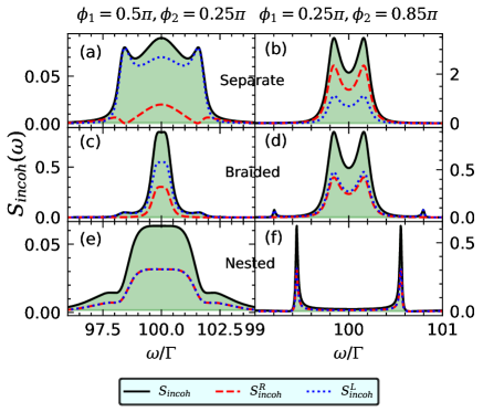
Figure 2: Incoherent power spectra in the three different configurations as a function of frequency $\omega$ with different values of $\phi_{1}$ and $\phi_{2}$. The first row corresponds to the separate case, the second row corresponds to the braided case, and the third row corresponds to the nested case. In addition, the black solid line denotes the total incoherent power spectrum, the red dashed line denotes the incoherent power spectrum in transmission, and the blue dotted line denotes the incoherent power spectrum in reflection. The other parameters are $k=\omega_{0}=100\Gamma$.

Under the assumption of a narrow bandwidth of incident photons, where the spectral width of the wave packet is significantly smaller than $\Gamma$, the wave packet can be approximated as a $\delta$ function. This implies that the incident photons have an equal frequency $k_{1}=k_{2}=k=E/2$. In this case, the incoherent power spectra, including transmission $S^{R,c}_{\text{incoh}}(\omega)$, reflection $S^{L,c}_{\text{incoh}}(\omega)$, and total spectrum $S^{c}_{\text{incoh}}(\omega)=\sum_{\alpha}S^{\alpha,c}_{\text{incoh}}(\omega)$ (transmission + reflection), are plotted in Fig. 2 as a function of $\omega$.

In the waveguide QED system with two small atoms, the incoherent power spectrum exhibits a doublet feature [42, 12, 13], which is a clear signature of the photon-mediated interaction between the atoms. It can be verified that the doublet’s location corresponds to the two real parts of the roots of the denominators in $A_{1}^{c}(\omega)$ and $A_{2}^{c}(\omega)$, under the condition of $\phi_{1}=0$. However, for the two giant atoms, the shape of the incoherent power spectrum can be adjusted by the accumulated phase shifts. Also, the structure of the incoherent power spectra can be explained by the roots of the denominators in $A_{1}^{c}(\omega)$ and $A_{2}^{c}(\omega)$, which are given by

$$\omega_{1}^{c}= E/2-\eta_{c}/2-i\tilde{\Gamma}_{c}/2,$$

$$\omega_{2}^{c}= E/2+\eta_{c}/2+i\tilde{\Gamma}_{c}/2$$ (34)

for $A_{1}^{c}(\omega)$, and

$$\omega_{3}^{c}= E/2-\eta_{c}/2+i\tilde{\Gamma}_{c}/2,$$

$$\omega_{4}^{c}= E/2+\eta_{c}/2-i\tilde{\Gamma}_{c}/2$$ (35)

for $A_{2}^{c}(\omega)$. Here, the real part determines the peak location, while the imaginary part determines the peak width. The magnitude of the peak is inversely proportional to the imaginary part. The roots corresponding to the given parameters in Fig. 2 are listed in the table 1. An important distinction compared to the case of a single giant atom is that the incoherent power spectra differ in the transmission and reflection in the separate and braided configuration. This results from the exchange of atomic excitations in atoms for right-moving and left-moving incident photons due to the parity symmetry $\hat{P}\hat{\sigma}_{j}\hat{P}^{\dagger}=\hat{\sigma}_{3-j}$. This behavior is also consistent with the small atoms system [42, 12, 13]. In the nested configuration, their incoherent power spectra are the same because of the unchanged atomic excitations for the right-moving and left-moving incident photons, in which the parity symmetry is $\hat{P}\hat{\sigma}_{j}\hat{P}^{\dagger}=\hat{\sigma}_{j}$.

Table 1: The roots of the denominators in $A_{1}^{c}(\omega)$ and $A_{2}^{c}(\omega)$ for the three configurations. The numerical values are expressed in units of $\Gamma$.

	$\phi_{1}=0.5\pi$, $\phi_{2}=0.25\pi$	$\phi_{1}=0.25\pi$, $\phi_{2}=0.85\pi$
	$\omega_{1}^{s}=101.7-0.3i$	$\omega_{1}^{s}=100.2-0.08i$
Separate	$\omega_{2}^{s}=98.3+0.3i$	$\omega_{2}^{s}=99.8+0.08i$
	$\omega_{3}^{s}=100.3-1.7i$	$\omega_{3}^{s}=101.2-3.3i$
	$\omega_{4}^{s}=99.7+1.7i$	$\omega_{4}^{s}=98.8+3.3i$
	$\omega_{1}^{b}=101.7-0.3i$	$\omega_{1}^{b}=100.2-0.08i$
Braided	$\omega_{2}^{b}=98.3+0.3i$	$\omega_{2}^{b}=99.8+0.08i$
	$\omega_{3}^{b}=99.7-0.3i$	$\omega_{3}^{b}=99.2-0.014i$
	$\omega_{4}^{b}=100.3+0.3i$	$\omega_{4}^{b}=100.8+0.014i$
	$\omega_{1}^{n}=98.4-1.4i$	$\omega_{1}^{n}=99-0.64i$
Nested	$\omega_{2}^{n}=101.6+1.4i$	$\omega_{2}^{n}=101+0.64i$
	$\omega_{3}^{n}=101.6-0.56i$	$\omega_{3}^{n}=100.6-0.013i$
	$\omega_{4}^{n}=98.4+0.56i$	$\omega_{4}^{n}=99.4+0.013i$

In the separate configuration shown in Fig. 2(a), there are peaks located at $101.7$ and $98.3$, which have relatively narrow widths due to their smaller imaginary parts. Additionally, a broader peak around $100$ emerges as a result of the overlapping peaks at $99.7$ and $100.3$. Consequently, it becomes feasible to generate photon pairs over a broad frequency range. In Fig. 2(b), the peaks are positioned at $99.8$ and $100.2$, both characterized by identical widths, whereas the peaks at $99.8$ and $101.2$ vanish due to the diminutive values of $Z_{2,4}^{s}$ for the given parameters, which are also divided by a large imaginary parts. In the braided configuration shown in Fig. 2(c), there are peaks located at $101.7$ and $98.3$. A little broader width around $100$ also takes shape due to the overlapping peaks at $99.7$ and $100.3$. In Fig. 2(d), four peaks appear at $100.2$, $99.8$, $99.2$, and $100.8$, respectively. The smaller peaks at $99.2$ and $100.8$ emerge because of the small values of $Z_{2,4}^{b}$ but divided by much smaller imaginary parts. In the nested configuration shown in Fig. 2(e), there are two slightly dips at $98.4$ and $101.6$. This arises from the fact that $Z_{1}^{n}$ and $Z_{3}^{n}$ exhibit opposite signs for the given parameters, akin to the destructive interference. The central broad peak is also formed from overlapping peaks contributed by $Z_{1}^{n}$ at $98.4$ and $101.6$, while contribution from $Z_{2}^{n}$ is negligible due to its small value. In Fig. 2(f), the peaks are located at $99.4$ and $100.6$ with narrower widths. The peaks at $99$ and $101$ disappear because of the small values of $Z_{1}^{n}$ for the given parameters but divided by a relatively large imaginary component.

Furthermore, the overall incoherent power spectrum is defined as

$$F^{c}(k)= \int d\omega S^{c}_{\text{incoh}}(\omega)$$

$$= \frac{2}{\pi}\int dx\left[\left|{B_{k_{1}k_{2}}^{RR,c}(x)}\right|^{2}+\left|{B_{k_{1}k_{2}}^{LL,c}(x)}\right|^{2}\right].$$ (36)

This provides a measure of the overall strength of correlations and a direct measurement of the bound-state term. When $k_{1}=k_{2}=k$, after integration, the expression for the overall incoherent power spectrum can be obtained as

$$F^{c}(k) =\frac{8}{\pi}\Bigg{[}\frac{\left|{Z_{1}^{c}}\right|^{2}+\left|{Z_{3}^{c}}\right|^{2}}{i\eta_{c}^{*}-i\eta_{c}+\tilde{\Gamma}_{c}^{*}+\tilde{\Gamma}_{c}}+\frac{\left|{Z_{2}^{c}}\right|^{2}+\left|{Z_{4}^{c}}\right|^{2}}{i\eta_{c}^{*}-i\eta_{c}-\tilde{\Gamma}_{c}^{*}-\tilde{\Gamma}_{c}}$$

$$+\frac{Z_{1}^{c*}Z_{2}^{c}+Z_{3}^{c*}Z_{4}^{c}}{i\eta_{c}^{*}-i\eta_{c}+\tilde{\Gamma}_{c}^{c*}-\tilde{\Gamma}_{c}}+\frac{Z_{1}^{c}Z_{2}^{c*}+Z_{3}^{c}Z_{4}^{c*}}{i\eta_{c}^{*}-i\eta_{c}-\tilde{\Gamma}_{c}^{*}+\tilde{\Gamma}_{c}}\Bigg{]}.$$ (37)

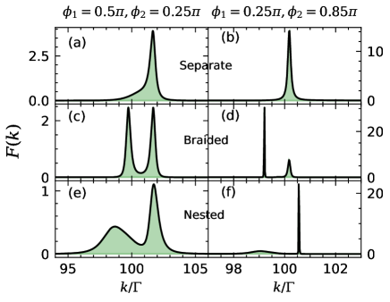
Figure 3: Overall incoherent power spectra in the three different configurations as a function of $k$ with different values of $\phi_{1}$ and $\phi_{2}$. The first row corresponds to the separate case, the second row corresponds to the braided case, and the third row corresponds to the nested case. The other parameter is $\omega_{0}=100\Gamma$.

The overall incoherent power spectra for the three configurations $F^{c}(k)$ as a function of the incident frequency $k$ is shown in Fig. 3. A large value of $F^{c}(k)$ indicates strong correlation effects, since the incoherent scattering arises from the correlation of the bound state. Therefore, the peak value indicates the strongest correlation, and the corresponding $k_{\text{peak}}$ represents the optimal incident frequency to obtain photon-photon correlation. The shape of $F^{c}(k)$ varies with the accumulated phase shifts $\phi_{1}$ and $\phi_{2}$. Physically, the position and width of the peaks can be explained by the poles of the system, which correspond to the roots of $D^{c}$. Denoting the poles as $z=\tilde{\omega}-i\tilde{\Gamma}$, the real part $\tilde{\omega}$ represents the eigenfrequency, and $\tilde{\Gamma}$ denotes the collective decay rate [47, 30]. The position of the peak aligns with the eigenfrequency $\tilde{\omega}$, while its width is determined by $\tilde{\Gamma}$. Moreover, the peak value is inversely proportional to $\tilde{\Gamma}$. In the separate configuration in Fig. 3(a), two poles are $100.3-1.7i$ and $101.7-0.3i$. Consequently, the primary peak is located at $101.7$, while the other peak is negligible due to its large imaginary part. In Fig. 3(b), the two poles are $101.2-3.3i$ and $100.2-0.08i$, leading to main peak being located at $100.2$ with a narrow width. Similarly, for the braided configuration in Fig. 3(c), the two poles are $99.7-0.3i$ and $101.7-0.3i$. Hence, there are two peaks located at $99.7$ and $101.7$, both with equal widths. Also, in Fig. 3(d), the poles correspond to $99.2-0.014i$ and $100.2-0.08i$. This results in the main peak being located at $99.2$ with a narrow width, while the other smaller peak is located at $100.2$. For the nested configuration in Fig. 3(e), the two poles are $101.6-0.56i$ and $98.4-1.43i$. So the main peak is located at $101.6$, while the other smaller peak is at $98.4$, exhibiting a wider width. In Fig. 3(f), the poles are $100.6-0.013i$ and $99-0.64i$. Hence the main peak is located at $100.6$ with a narrow width, while the other negligible peak is located at $99$.

VI Second-order correlation function

Next, we utilize the second-order correlation function to demonstrate the spatial interaction between photons [52]. The second-order correlation functions of the transmitted and reflected fields ($x_{1}>d/2$, $x_{2}>d/2$ and $x=x_{2}-x_{1}$) are defined as follows:

$${G_{\alpha}^{c}}^{(2)}(x)= \left\langle{\Psi_{2}^{c}}\right|\hat{a}^{\dagger}_{\alpha}(x_{1})\hat{a}^{\dagger}_{\alpha}(x_{2})\hat{a}_{\alpha}(x_{2})\hat{a}_{\alpha}(x_{1})\left|{\Psi_{2}^{c}}\right\rangle$$

$$=2\left|{f_{\alpha\alpha}^{c}(x_{1},x_{2})}\right|^{2}.$$ (38)

This correlation function represents the probability of detecting a photon at $x_{2}$ after detecting the first one at $x_{1}$. The expression is directly proportional to the rate at which two photons are transmitted or reflected, and is determined by the interference between the plane-wave term and the bound-state term. In order to briefly illustrate the effect of the bound state, we examine the second-order differential correlaiton function [53, 54, 55, 56], which is the difference between the probability of two-photon detection and the independent single-photon detection when $x=0$. Concretely, under the condition that $k_{1}=k_{2}=k$, the differential correlation function are

$$\chi_{R}^{c}=2\pi^{2}\left|{f_{RR}^{c}(0)}\right|^{2}-\left|{t_{2}^{c}(k)}\right|^{4}$$ (39)

for the transmitted field and

$$\chi_{L}^{c}=2\pi^{2}\left|{f_{LL}^{c}(0)}\right|^{2}-\left|{r_{1}^{c}(k)}\right|^{4}$$ (40)

for the reflected field. If $\chi_{R}>0$, it indicates that the bound state enhances the transmission of two photons, resulting in a phenomenon known as photon-induced tunneling, which serves as a signature of photon bunching. Conversely, if $\chi_{R}<0$, it implies that the bound state can suppress the transmission of two photons, leading to photon blockade [57, 58]. The second-order differential correlation functions for the three configurations are numerically plotted in Fig. 4.

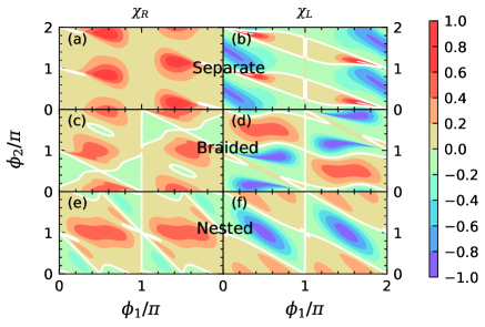
Figure 4: Second-order differential correlation functions in the three different configurations as functions of $\phi_{1}$ and $\phi_{2}$. The first row corresponds to the separate configuration, the second row corresponds to the braided configuration, and the third row corresponds to the nested configuration. Moreover, the first column represents the transmission, and the second column represents the reflection. The white lines indicate that the differential correlation functions equal to zero. The other parameters are $k=\omega_{0}=100\Gamma$.

Although the photon correlation can be enhanced by adjusting the phase shift for the single giant atom, it is unable to switch between bunching and antibunching [59]. This limitation arises because a single two-level atom can absorb only one photon at a time and cannot emit two photons simultaneously. Hence, in the case of reflection from a single giant atom, the second-order correlation function $g^{(2)}(0)=0$. However, this constraint can be overcome by incorporating additional two-level atoms, as it allows for the tuning of $g^{(2)}(0)$. The presence of multiple two-level atoms enables the possibility of one photon being absorbed by the first atom while the other photon propagates to the subsequent atom and gets reflected, thereby triggering the stimulated emission of the first photon. As a result, the probability of two photons being emitted together is not completely suppressed. This phenomenon becomes even more pronounced when two giant atoms are present. In the case of transmission for the two giant atoms, we find that the transmitted photons exhibit bunching behavior when the atoms are in the separate configuration, similar to small atoms. However, the transmitted photons can display either bunching or antibunching behavior by adjusting the phase shifts $\phi_{1}$ and $\phi_{2}$ in the braided and nested cases. As for the reflection, the reflected photons can exhibit either bunching or antibunching behavior by adjusting the phase shifts $\phi_{1}$ and $\phi_{2}$ in all three cases.

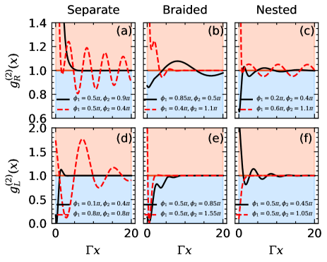
Figure 5: Normalized second-order correlation functions in the three different configurations as a function of $x$ with different values of $\phi_{1}$ and $\phi_{2}$. The first row corresponds to the transmission, and the second row corresponds to the reflection. Additionally, the first column represents the separate case, the second column represents the braided case, and the third column represents the nested case. The other parameters are $k=\omega_{0}=100\Gamma$.

The differential correlation function provides a clear measure of the probability of generating two photons simultaneously. However, it is less sensitive to single-photon transmission and reflection. To address this, it is helpful to introduce the normalized second-order correlation function [44, 60, 61, 62]

$${g_{\alpha}^{c}}^{(2)}(x)=\frac{{G^{c}_{\alpha}}^{(2)}(x)}{\left|{{}_{\alpha}\langle x_{1}\left|{\Phi_{1}^{c}(k_{1})}\right\rangle_{R}}\right|^{2}\left|{{}_{\alpha}\langle x_{2}\left|{\Phi_{1}^{c}(k_{2})}\right\rangle_{R}}\right|^{2}}.$$ (41)

This function is normalized by the single-photon transmission and reflection probabilities. After performing calculations, the normalized second-order correlation functions in transmission and reflection can be expressed in the form

$${g_{R}^{c}}^{(2)}(x)= \bigg{|}1+\frac{Z_{1}^{c}}{t_{4}^{c}(k_{1})t_{4}^{c}(k_{2})}e^{(i\eta_{c}-\tilde{\Gamma}_{c})\left|{x}\right|/2}$$

$$+\frac{Z_{2}^{c}}{t_{4}^{c}(k_{1})t_{4}^{c}(k_{2})}e^{(i\eta_{c}+\tilde{\Gamma}_{c})\left|{x}\right|/2}\bigg{|}^{2},$$

$${g_{L}^{c}}^{(2)}(x)= \bigg{|}1+\frac{Z_{3}^{c}}{r_{1}^{c}(k_{1})r_{1}^{c}(k_{2})}e^{(i\eta_{c}-\tilde{\Gamma}_{c})\left|{x}\right|/2}$$

$$+\frac{Z_{4}^{c}}{r_{1}^{c}(k_{1})r_{1}^{c}(k_{2})}e^{(i\eta_{c}+\tilde{\Gamma}_{c})\left|{x}\right|/2}\bigg{|}^{2}.$$ (42)

These correlation functions are shown in Fig. 5. Here we choose the frequency of the input field to be resonant with the atomic transition frequency, i.e., $k_{1}=k_{2}=k=\omega_{0}$. It should be noted that, consistent with Fig. 4, in Fig 5(a), the transmission correlations both exhibit bunching behavior (${g_{R}^{s}}^{(2)}(0)>0$) in the separate configuration. However, in the braided and nested configurations shown in Figs. 5(b) and (c), the initial bunching ${g_{R}^{b/n}}^{(2)}(0)>0$ and antibunching ${g_{R}^{b/n}}^{(2)}(0)<0$ can be manipulated by adjusting the phase shifts $\phi_{1}$ and $\phi_{2}$. As for reflection, the correlation can either display bunching or antibunching behavior in all three configurations by adjusting the phase shifts.

Besides, it is important to note that the initial value ${g_{\alpha}^{c}}^{(2)}(x)$ cannot predict the overall photon-photon correlation due to the complex nature of the function. This complexity arises from the beating between the incident frequency and the two eigenfrequencies $(\eta_{c}\pm i\tilde{\Gamma}_{c})/2$, which correspond to the complete set of collective decay rates [47, 30]. The long-distance behavior is determined by the most sub-radiant pole [42]. For example, in the separate configuration shown in Fig. 5(a), the imaginary of the most sub-radiant pole is $0.7$ for $\phi_{1}=0.5\pi$ and $\phi_{2}=0.9\pi$ (black solid line), while it is $0.05$ for $\phi_{1}=0.5\pi$ and $\phi_{2}=0.4\pi$ (red-dashed line), which exhibits the long-distance oscillation. A similar analysis can be applied to the other sub-figures as well. In the limit of large $x$, the contribution of the bound state becomes negligible, and the second-order correlation function approaches to $1$.

VII Conclusions

In conclusion, we have instigated the two-photon scattering processes involving two giant atoms coupled to a 1D waveguide. We study three different configurations including the separate, braided, and nested using the LS formalism. The approach enables us to obtain analytical expressions for the two-photon interacting scattering wavefunctions under the Markovian approximation. Based on the analytical results, we further derive the incoherent power spectrum arising from the correlation of the bound state, which characterizes the generation of correlated photon pairs. Distinct from small atoms, we find the presence of more peak values and a broader frequency band. Furthermore, the total flux serving as a measure of photon-photon correlation, can be modified by the phase shifts, and explained by the poles of the system. The second-order correlation function provides a direct measure of photon-photon correlation, and our analysis reveal that the accumulated phase shifts can be effectively utilized to qualitatively tune the photon-photon correlation, such as manipulating of either initial bunching or initial antibunching behavior in the transmission and reflection. Lastly, the long-distance evolution of the second-order correlation is possible from the most sub-radiant poles. This work offers possiblities for generating tunable nonclassical photon source, which may have potential applications in the construction of quantum networks based on the giant-atom waveguide-QED systems.

References

• Lodahl et al. [2015] P. Lodahl, S. Mahmoodian, and S. Stobbe, Interfacing single photons and single quantum dots with photonic nanostructures, Rev. Mod. Phys. 87, 347 (2015).
• Facchi et al. [2016] P. Facchi, M. S. Kim, S. Pascazio, F. V. Pepe, D. Pomarico, and T. Tufarelli, Bound states and entanglement generation in waveguide quantum electrodynamics, Phys. Rev. A 94, 043839 (2016).
• Kimble [2008] H. J. Kimble, The quantum internet, Nature 453, 1023 (2008).
• Bermel et al. [2006] P. Bermel, A. Rodriguez, S. G. Johnson, J. D. Joannopoulos, and M. Soljačić, Single-photon all-optical switching using waveguide-cavity quantum electrodynamics, Phys. Rev. A 74, 043818 (2006).
• Kannan et al. [2020a] B. Kannan, D. L. Campbell, F. Vasconcelos, R. Winik, D. K. Kim, M. Kjaergaard, P. Krantz, A. Melville, B. M. Niedzielski, J. L. Yoder, T. P. Orlando, S. Gustavsson, and W. D. Oliver, Generating spatially entangled itinerant photons with waveguide quantum electrodynamics, Science Advances 6, eabb8780 (2020a).
• Politi et al. [2008] A. Politi, M. J. Cryan, J. G. Rarity, S. Yu, and J. L. O’Brien, Silica-on-silicon waveguide quantum circuits, Science 320, 646 (2008).
• Mirhosseini et al. [2019] M. Mirhosseini, E. Kim, X. Zhang, A. Sipahigil, P. B. Dieterle, A. J. Keller, A. Asenjo-Garcia, D. E. Chang, and O. Painter, Cavity quantum electrodynamics with atom-like mirrors, Nature 569, 692 (2019).
• Kannan et al. [2023] B. Kannan, A. Almanakly, Y. Sung, A. Di Paolo, D. A. Rower, J. Braumüller, A. Melville, B. M. Niedzielski, A. Karamlou, K. Serniak, A. Vepsäläinen, M. E. Schwartz, J. L. Yoder, R. Winik, J. I.-J. Wang, T. P. Orlando, S. Gustavsson, J. A. Grover, and W. D. Oliver, On-demand directional microwave photon emission using waveguide quantum electrodynamics, Nature Physics 19, 394 (2023).
• Sheremet et al. [2023] A. S. Sheremet, M. I. Petrov, I. V. Iorsh, A. V. Poshakinskiy, and A. N. Poddubny, Waveguide quantum electrodynamics: Collective radiance and photon-photon correlations, Rev. Mod. Phys. 95, 015002 (2023).
• Hoi et al. [2011] I.-C. Hoi, C. M. Wilson, G. Johansson, T. Palomaki, B. Peropadre, and P. Delsing, Demonstration of a single-photon router in the microwave regime, Phys. Rev. Lett. 107, 073601 (2011).
• Hoi et al. [2013] I.-C. Hoi, C. M. Wilson, G. Johansson, J. Lindkvist, B. Peropadre, T. Palomaki, and P. Delsing, Microwave quantum optics with an artificial atom in one-dimensional open space, New Journal of Physics 15, 025011 (2013).
• Lalumière et al. [2013] K. Lalumière, B. C. Sanders, A. F. van Loo, A. Fedorov, A. Wallraff, and A. Blais, Input-output theory for waveguide qed with an ensemble of inhomogeneous atoms, Phys. Rev. A 88, 043806 (2013).
• van Loo et al. [2013] A. F. van Loo, A. Fedorov, K. Lalumière, B. C. Sanders, A. Blais, and A. Wallraff, Photon-mediated interactions between distant artificial atoms, Science 342, 1494 (2013).
• Nie et al. [2021] W. Nie, T. Shi, F. Nori, and Y.-x. Liu, Topology-enhanced nonreciprocal scattering and photon absorption in a waveguide, Phys. Rev. Appl. 15, 044041 (2021).
• Dong et al. [2021] Y. Dong, J. Taylor, Y. S. Lee, H. R. Kong, and K. S. Choi, Waveguide-qed platform for synthetic quantum matter, Phys. Rev. A 104, 053703 (2021).
• Shi and Fan [2013] T. Shi and S. Fan, Two-photon transport through a waveguide coupling to a whispering-gallery resonator containing an atom and photon-blockade effect, Phys. Rev. A 87, 063818 (2013).
• Poshakinskiy and Poddubny [2016] A. V. Poshakinskiy and A. N. Poddubny, Biexciton-mediated superradiant photon blockade, Phys. Rev. A 93, 033856 (2016).
• Roy [2010] D. Roy, Few-photon optical diode, Phys. Rev. B 81, 155117 (2010).
• Roy [2011a] D. Roy, Two-photon scattering by a driven three-level emitter in a one-dimensional waveguide and electromagnetically induced transparency, Phys. Rev. Lett. 106, 053601 (2011a).
• Gu et al. [2022] W.-j. Gu, L. Wang, Z. Yi, and L.-h. Sun, Generation of nonreciprocal single photons in the chiral waveguide-cavity-emitter system, Phys. Rev. A 106, 043722 (2022).
• Yi et al. [2023] Z. Yi, H. Huang, Y. Yan, L. Sun, and W. Gu, Correlated two-photon scattering in a 1d waveguide coupled to an n-type four-level emitter, Annalen der Physik 535, 2200512 (2023).
• Shen and Fan [2007a] J.-T. Shen and S. Fan, Strongly correlated two-photon transport in a one-dimensional waveguide coupled to a two-level system, Phys. Rev. Lett. 98, 153003 (2007a).
• Kannan et al. [2020b] B. Kannan, M. J. Ruckriegel, D. L. Campbell, A. Frisk Kockum, J. Braumüller, D. K. Kim, M. Kjaergaard, P. Krantz, A. Melville, B. M. Niedzielski, A. Vepsäläinen, R. Winik, J. L. Yoder, F. Nori, T. P. Orlando, S. Gustavsson, and W. D. Oliver, Waveguide quantum electrodynamics with superconducting artificial giant atoms, Nature 583, 775 (2020b).
• Gustafsson et al. [2014] M. V. Gustafsson, T. Aref, A. F. Kockum, M. K. Ekström, G. Johansson, and P. Delsing, Propagating phonons coupled to an artificial atom, Science 346, 207 (2014).
• Vadiraj et al. [2021] A. M. Vadiraj, A. Ask, T. G. McConkey, I. Nsanzineza, C. W. S. Chang, A. F. Kockum, and C. M. Wilson, Engineering the level structure of a giant artificial atom in waveguide quantum electrodynamics, Phys. Rev. A 103, 023710 (2021).
• Frisk Kockum et al. [2014] A. Frisk Kockum, P. Delsing, and G. Johansson, Designing frequency-dependent relaxation rates and lamb shifts for a giant artificial atom, Phys. Rev. A 90, 013837 (2014).
• Andersson et al. [2019] G. Andersson, B. Suri, L. Guo, T. Aref, and P. Delsing, Non-exponential decay of a giant artificial atom, Nature Physics 15, 1123 (2019).
• Longhi [2020] S. Longhi, Photonic simulation of giant atom decay, Opt Lett 45, 3017 (2020).
• Guo et al. [2020a] S. Guo, Y. Wang, T. Purdy, and J. Taylor, Beyond spontaneous emission: Giant atom bounded in the continuum, Phys. Rev. A 102, 033706 (2020a).
• Qiu et al. [2023] Q.-Y. Qiu, Y. Wu, and X.-Y. Lü, Collective radiance of giant atoms in non-markovian regime, Science China Physics, Mechanics & Astronomy 66, 224212 (2023).
• Guo et al. [2020b] L. Guo, A. F. Kockum, F. Marquardt, and G. Johansson, Oscillating bound states for a giant atom, Phys. Rev. Res. 2, 043014 (2020b).
• Kockum et al. [2018] A. F. Kockum, G. Johansson, and F. Nori, Decoherence-free interaction between giant atoms in waveguide quantum electrodynamics, Phys. Rev. Lett. 120, 140404 (2018).
• Carollo et al. [2020] A. Carollo, D. Cilluffo, and F. Ciccarello, Mechanism of decoherence-free coupling between giant atoms, Phys. Rev. Res. 2, 043184 (2020).
• Santos and Bachelard [2023] A. C. Santos and R. Bachelard, Generation of maximally entangled long-lived states with giant atoms in a waveguide, Phys. Rev. Lett. 130, 053601 (2023).
• Yin et al. [2022] X.-L. Yin, W.-B. Luo, and J.-Q. Liao, Non-markovian disentanglement dynamics in double-giant-atom waveguide-qed systems, Phys. Rev. A 106, 063703 (2022).
• Yin and Liao [2023] X.-L. Yin and J.-Q. Liao, Generation of two-giant-atom entanglement in waveguide-qed systems, Phys. Rev. A 108, 023728 (2023).
• Feng and Jia [2021] S. L. Feng and W. Z. Jia, Manipulating single-photon transport in a waveguide-qed structure containing two giant atoms, Phys. Rev. A 104, 063712 (2021).
• Peng and Jia [2023] Y. P. Peng and W. Z. Jia, Single-photon scattering from a chain of giant atoms coupled to a one-dimensional waveguide, Phys. Rev. A 108, 043709 (2023).
• Zhou et al. [2023] J. Zhou, X.-L. Yin, and J.-Q. Liao, Chiral and nonreciprocal single-photon scattering in a chiral-giant-molecule waveguide-qed system, Phys. Rev. A 107, 063703 (2023).
• Shen and Fan [2007b] J.-T. Shen and S. Fan, Strongly correlated multiparticle transport in one dimension through a quantum impurity, Phys. Rev. A 76, 062709 (2007b).
• Chang et al. [2007] D. E. Chang, A. S. Sørensen, E. A. Demler, and M. D. Lukin, A single-photon transistor using nanoscale surface plasmons, Nature Physics 3, 807 (2007).
• Fang and Baranger [2015] Y.-L. L. Fang and H. U. Baranger, Waveguide qed: Power spectra and correlations of two photons scattered off multiple distant qubits and a mirror, Phys. Rev. A 91, 053845 (2015).
• Zheng and Baranger [2013a] H. Zheng and H. U. Baranger, Persistent quantum beats and long-distance entanglement from waveguide-mediated interactions, Phys. Rev. Lett. 110, 113601 (2013a).
• Fang et al. [2014] Y.-L. L. Fang, H. Zheng, and H. U. Baranger, One-dimensional waveguide coupled to multiple qubits: photon-photon correlations, EPJ Quantum Technology 1, 3 (2014).
• Roy [2011b] D. Roy, Correlated few-photon transport in one-dimensional waveguides: Linear and nonlinear dispersions, Phys. Rev. A 83, 043823 (2011b).
• Roy et al. [2017] D. Roy, C. M. Wilson, and O. Firstenberg, Colloquium: Strongly interacting photons in one-dimensional continuum, Rev. Mod. Phys. 89, 021001 (2017).
• Dinc et al. [2019] F. Dinc, İ. Ercan, and A. M. Brańczyk, Exact Markovian and non-Markovian time dynamics in waveguide QED: collective interactions, bound states in continuum, superradiance and subradiance, Quantum 3, 213 (2019).
• Zheng and Baranger [2013b] H. Zheng and H. U. Baranger, Persistent quantum beats and long-distance entanglement from waveguide-mediated interactions, Phys. Rev. Lett. 110, 113601 (2013b).
• Guo et al. [2017] L. Guo, A. Grimsmo, A. F. Kockum, M. Pletyukhov, and G. Johansson, Giant acoustic atom: A single quantum system with a deterministic time delay, Phys. Rev. A 95, 053821 (2017).
• Xu et al. [2013a] S. Xu, E. Rephaeli, and S. Fan, Analytic properties of two-photon scattering matrix in integrated quantum systems determined by the cluster decomposition principle, Phys. Rev. Lett. 111, 223602 (2013a).
• Law et al. [2000] C. K. Law, I. A. Walmsley, and J. H. Eberly, Continuous frequency entanglement: Effective finite hilbert space and entropy control, Phys. Rev. Lett. 84, 5304 (2000).
• Loudon [2000] R. Loudon, The quantum theory of light (Oxford University Press, 2000).
• Kubanek et al. [2008] A. Kubanek, A. Ourjoumtsev, I. Schuster, M. Koch, P. W. H. Pinkse, K. Murr, and G. Rempe, Two-photon gateway in one-atom cavity quantum electrodynamics, Phys. Rev. Lett. 101, 203602 (2008).
• Majumdar et al. [2012] A. Majumdar, M. Bajcsy, and J. Vučković, Probing the ladder of dressed states and nonclassical light generation in quantum-dot–cavity qed, Phys. Rev. A 85, 041801 (2012).
• Xu et al. [2013b] X.-W. Xu, Y.-J. Li, and Y.-x. Liu, Photon-induced tunneling in optomechanical systems, Phys. Rev. A 87, 025803 (2013b).
• Kowalewska-Kudłaszyk et al. [2019] A. Kowalewska-Kudłaszyk, S. I. Abo, G. Chimczak, J. Peřina, F. Nori, and A. Miranowicz, Two-photon blockade and photon-induced tunneling generated by squeezing, Phys. Rev. A 100, 053857 (2019).
• Zheng et al. [2011] H. Zheng, D. J. Gauthier, and H. U. Baranger, Cavity-free photon blockade induced by many-body bound states, Phys. Rev. Lett. 107, 223601 (2011).
• Zheng et al. [2012] H. Zheng, D. J. Gauthier, and H. U. Baranger, Strongly correlated photons generated by coupling a three- or four-level system to a waveguide, Phys. Rev. A 85, 043832 (2012).
• Gu et al. [2023] W. Gu, H. Huang, Z. Yi, L. Chen, L. Sun, and H. Tan, Correlated two-photon scattering in a 1d waveguide coupled to two- or three-level giant atoms, arXiv:2306.13836  (2023), preprint.
• Vinu and Roy [2023] A. Vinu and D. Roy, Single photons versus coherent-state input in waveguide quantum electrodynamics: Light scattering, kerr, and cross-kerr effect, Phys. Rev. A 107, 023704 (2023).
• Vinu and Roy [2020] A. Vinu and D. Roy, Amplification and cross-kerr nonlinearity in waveguide quantum electrodynamics, Phys. Rev. A 101, 053812 (2020).
• Liang et al. [2018] Q.-Y. Liang, A. V. Venkatramani, S. H. Cantu, T. L. Nicholson, M. J. Gullans, A. V. Gorshkov, J. D. Thompson, C. Chin, M. D. Lukin, and V. Vuletić, Observation of three-photon bound states in a quantum nonlinear medium, Science 359, 783 (2018).