On convergence analysis of feedback control with integral action and discontinuous relay perturbation

Abstract

We consider third-order dynamic systems which have integral feedback action and discontinuous relay disturbance. More specifically for applications, our focus is on the integral plus state-feedback control of motion systems with discontinuous Coulomb-type friction. We resume the attractive stiction region, where the hybrid system has also solutions in Filippov sense and the motion trajectories remain in an idle state (that we call ‘stiction’) until the sliding-mode condition becomes violated by an integral action. We analyze the conditions for occurrence of the slowly converging stick-slip cycles. We also show that the hybrid system is globally but only asymptotically and almost always not exponentially stable. A particular case of exponential convergence can appear for some initial values, assuming the characteristic equation of the linear subsystem has only the real roots. Illustrative numerical examples are provided alongside with the developed analysis.

I Introduction

Discontinuous relays in feedback are frequently appearing in dynamic systems, thus leading to the (hybrid) switching systems, cf. e.g. [17], and as a particular class to the systems with sliding modes, cf. e.g. [11]. The latter require usually the solutions in Filippov’s sense [5] of the differential equations with discontinuous right-hand-side – the methodology of which we will make use also in the present study. Several works considered extensively both, existence of the fast switches and limit cycles in relay feedback systems, see [15, 16]. It has been discussed, e.g. in [16], that ‘if the linear part of the relay feedback system has pole excess one and certain other conditions are fulfilled, then the system has a limit cycle with sliding mode.’ At the same time, a very common application example of the integral plus state-feedback control of the motion systems with discontinuous Coulomb-type friction has pole excess one, while being usually understood as globally asymptotically stable for the properly assigned linear feedback gains, see e.g. [3, 4, 9]. The complex, and rather parasitic, effects of friction on the feedback controlled dynamic systems are since long studied in systems and control communities, see e.g. [2]. The summarized basics of kinetic friction affecting the feedback controlled systems can be found, for instance, in the recent work [10]. Also experimental studies disclosing the impact of Coulomb friction in vicinity to the control settling point, e.g. [8], can be viewed for traceability. How a feedback controlled second-order system (i.e. without integral control action) comes to the so-called sticking due to the relay-type Coulomb friction was analyzed in [1]. A possible appearance of the friction-induced limit cycles were formerly addressed in e.g. [7, 6]. The source of such persistent limit cycles is, however, not trivial and requires more than the relay-type Coulomb friction. According to the focused studies [3, 4, 9], the global asymptotic stability of a proportional-integral-derivative controlled system with relay-type Coulomb friction is given, and the slowly converging stick-slip cycles appear instead of persistent limit cycles.

Given the above background, the present work aims to further contribute to the convergence analysis of feedback control with integral action when a discontinuous relay occurs in feedback as a known perturbation. Below, the problem statement is formulated, followed by the main results placed in section II. The dedicated illustrative numerical examples are provided in section III. Section IV summarizes the paper and highlight several points for discussion. The particular solutions in use are detailed in Appendix.

Problem statement

We consider the following class of third-order systems

$$\dddot{y}(t)+a\,\ddot{y}(t)+b\,\dot{y}(t)+c\,y(t)=-\gamma\,\mathrm{sign}(\ddot{y}(t)),$$ (1)

where $a,\,b,\,c>0$ are the design parameters, and $\gamma>0$ is the gain of the discontinuous relay function assumed to be known. The latter, described by the sign operator, is defined in the Filippov sense [5] on the closed interval in zero, i.e.

$$\mathrm{sign}(z)=\left\{\begin{array}[]{ll}1,&\;z>0,\\ \left[-1,1\right],&\;z=0,\\ -1,&\;z<0.\\ \end{array}\right.$$ (2)

Remark 1

The system class (1) can equally describe the second-order state-feedback controlled motion with discontinuous Coulomb friction, cf. [9, 10], and integral output regulation. This case, the constants $a$ and $b$ capture both, the state feedback gains and structural parameters of a motion system, while $c$ and $\gamma$ contain the integral feedback gain and the Coulomb friction coefficient, respectively. Moreover, all parameters are normalized by a positive inertial mass.

Further we note that generally

$$y(0)=C_{1},\quad\dot{y}(0)=C_{2},\quad\ddot{y}(0)=C_{3},$$ (3)

where $C_{1},C_{2},C_{3}\in\mathbb{R}$, while for an application case $C_{1}=C_{3}=0$ and $C_{2}\neq 0$ are often assumed. The objectives targeted in the following are to

1. provide a simple prove of the global asymptotic stability (GAS), cf. with [4, 9], of the system (1) and show the parametric conditions that guarantee GAS property;

2. provided (i), to show where (in state-space) and when the system (1) becomes transiently sticking, i.e. $\ddot{y}(t)=0$ for all $t\in[t_{i}^{s},\,t_{i}^{c}]$ with $0\leq t_{i}^{s}<t_{i}^{c}<\infty$ and $i\in\mathbb{N}^{+}$, and how it depends on the system parameters;

3. provided (i) and (ii), to analyze the asymptotic convergence in period stick-slip cycles, while a slipping phase is characterized by $\ddot{y}(t)\neq 0$ for all $t\in[t_{i}^{c},\,t_{i+1}^{s}]$ with $0\leq t_{i}^{c}<t_{i+1}^{s}<\infty$.

II Main results

II-A Global asymptotic stability

From the structural viewpoint, the system (1) can be represented as a feedback loop with the discontinuous relay (2) as shown in Fig. 1. The linear subsystem

$$G(s)=\frac{y(s)s^{2}}{u(s)}=C(sI-A)^{-1}B$$ (4)

is third-order and minimum-phase, with

$$A=\left(\begin{array}[]{ccc}0&1&0\\ 0&0&1\\ -c&-b&-a\\ \end{array}\right),B=\left(\begin{array}[]{c}0\\ 0\\ \gamma\\ \end{array}\right),C^{\top}=\left(\begin{array}[]{c}0\\ 0\\ 1\\ \end{array}\right),$$ (5)

which are the system matrix and input and output coupling vectors, respectively. The $3\times 3$ identity matrix is denote by $I$, and $s$ is obviously the complex Laplace variable. The corresponding state-space vector is $x\equiv[x_{1},\,x_{2},\,x_{3}]^{\top}=[y,\,\dot{y},\,\ddot{y}]^{\top}$. Note that the feedback relay acts as an input perturbation of $G(s)$.

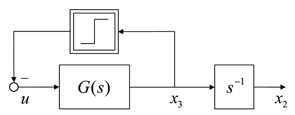
Figure 1: Structure of the third-order system with feedback relay perturbation.

We are now in the position to formulate and prove the GAS properties of the system (1), (2).

Theorem 1

The system (1), (2) with $a,\,b,\,c,\,\gamma>0$ is globally asymptotically stable if

$$ab>c.$$ (6)

Proof:

The proof is carried out by showing the strict passivity of the system (4), (5) with the input $u=-\mathrm{sign}(x_{3})$ and output $v=x_{3}$. Such input-output system is said to be strictly passive if, cf. [12, Definition 6.3],

$$uv\geq\dot{V}+\psi(x)$$ (7)

is valid for some positive definite function $\psi(x)$ and continuously differentiable positive semidefinite function $V(x)$, which is called the storage function. Without loss of generality, assume a quadratic Lyapunov function

$$V(x)=x^{\top}Px\quad\hbox{with}\quad P=P^{\top}.$$ (8)

Let us use the fact that if $A$ is Hurwitz, i.e.

$$\mathrm{Re}\{\lambda_{j}\}<0$$

for all eigenvalues $\lambda_{j}$ of $A$, then $P$ is the unique solution of

$$PA+A^{\top}P=-Q,$$ (9)

for a given positive definite symmetric matrix $Q$, cf. [12, Theorem 4.6] and [13, Lemma 4.28]. In other words, let us find a positive definite symmetric matrix $P$ satisfying (9). One can show that assuming $Q=I$, the Lyapunov equation (9) has the analytic solution $P$, given in Appendix A. Now, following [12, Theorem 4.6], let us derive the parametric conditions for which $A$ is Hurwitz, which is then that implying the found $P$ is the unique solution of (9) and, also, positive definite. Applying the algebraic criterion of Routh-Hurwitz (cf. e.g. [14]) to the characteristic polynomial

$$s^{3}+as^{2}+bs+c=0$$ (10)

of the system (4), (5), one obtains (6). Then, substituting the time derivative of the Lyapunov function (8), i.e. $\dot{V}=-x^{\top}Qx$, into (7) and evaluating $uv$ we obtain

$$-|x_{3}|\geq-x_{1}^{2}-x_{2}^{2}-x_{3}^{2}+\psi(x).$$ (11)

Owing to the quadratic terms on the right-hand-side of (11), there is always some positive definite function $\psi(x)$ so that (11) holds for all $x\in\mathbb{R}^{3}$. This proves the feedback system (4), (5) as in Fig. 1, and so also (1), (2), is strictly passive. Therefore, since the storage function $V(x)$ is radially unbounded, cf. (8), the system (1), (2) is also globally asymptotically stable in accord with [12, Lemma 6.7]. ∎

Remark 2

Note that the GAS condition (6) is conservative, since the passive relay in feedback, cf. Fig. 1, provides an additional system damping, i.e. energy dissipation in $\dot{V}(t)$, during each slipping phase defined by (iii) in section I.

II-B Properties of stiction region

Despite the system (1), (2) proved to be GAS, when the Theorem 1 is satisfied, the $(x_{2},x_{3})$ trajectories can temporarily come to stiction, i.e. $x_{3}=0$, due to the impact of switching relay, cf. [9]. Defining the switching surface

$$S=Cx(t)=0,$$ (12)

the state trajectories can either cross it or stay on it (i.e. being in a sliding-mode) depending on the vector fields of the corresponding differential inclusion, cf. [17],

$$\dot{x}\in F(x)\equiv Ax-B\,\mathrm{sign}(x_{3}).$$ (13)

in vicinity of $S$. Here the relay value depends on whether $x\rightarrow S$ from $x\in\mathbb{R}^{3}_{+}\equiv\{\mathbb{R}^{3}\backslash S\,:\>x_{3}>0\}$ or from $x\in\mathbb{R}^{3}_{-}\equiv\{\mathbb{R}^{3}\backslash S\,:\>x_{3}<0\}$. Let us establish the condition and prove the appearance of the sliding-mode for (1), (2).

Theorem 2

The system (1), (2) with $a,\,b,\,c,\,\gamma>0$ is sticking when $\ddot{y}=0$ and has an unique solution in the Filippov sense [5] if and only if

$$\gamma>\bigl{|}b\dot{y}+cy\bigr{|}.$$ (14)

Proof:

The proof is carried out by using the standard existence condition for the sliding-modes. The state vector notation $x(t)$, defined in section II-A, will be further used instead of the $y(t)$ variable and its derivatives.

Excluding the global attractiveness property (that will be analyzed later) we use the condition

$$S\dot{S}<0\quad\hbox{for}\quad S\neq 0,$$

and more specifically the sufficient condition

$$\underset{S\rightarrow 0^{+}}{\lim}\,\dot{S}<0\quad\hbox{and}\quad\underset{S\rightarrow 0^{-}}{\lim}\,\dot{S}>0$$ (15)

for the sliding-mode to exist, cf. [18]. Taking the time derivative of (12) and evaluating it we obtain

$$\dot{S}=-\bigl{(}ax_{3}+bx_{2}+cx_{1}+\gamma\,\mathrm{sign}(x_{3})\bigr{)}.$$ (16)

Substituting (16) into (15) and evaluating both limits, while $\mathrm{sign}(S)=\mathrm{sign}(x_{3})$, results in

$$\gamma>\left\{\begin{array}[]{ll}-(bx_{2}+cx_{1}),&\hbox{ if }S\rightarrow 0^{+},\\[2.84526pt] bx_{2}+cx_{1},&\hbox{ if }S\rightarrow 0^{-}.\end{array}\right.$$ (17)

The inequality (17) is equivalent to (14) for $S=0$ when $x_{3}\equiv\ddot{y}=0$; that completes the proof. ∎

Remark 3

The derived condition (14) is equivalent to the set of attraction $\{x\in S:|CAx|<|CB|\}$ if $CB>0$ in a relay feedback system; the latter was demonstrated in [15, Section 4] in context of a necessary and sufficient condition for the system to have consecutive fast relay switches.

The parametric condition (14) is graphically well interpretable as shown in Fig. 2.

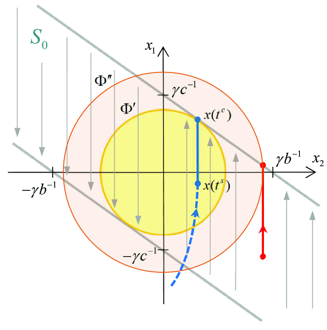
Figure 2: Stiction region $S_{0}$ in $\bigl{(}x_{2},x_{1}\bigr{)}$ coordinates.

The stiction region

$$S_{0}\equiv\{x\in\mathbb{R}^{3}\,:\>x_{3}=0,\,|bx_{2}+cx_{1}|<\gamma\}$$ (18)

lies in the $(x_{2},x_{1})$ plane, bounded by two straight lines which cross the $x_{2}$ and $x_{1}$ axes in $\pm\gamma b^{-1}$ and $\pm\gamma c^{-1}$, respectively. During the system sticking, the vector field $F$ is: (i) lying between both lines satisfying (18), (ii) orthogonal to $x_{2}$-axis, and (iii) unambiguously directed towards the growing $x_{1}$ values for $x_{2}>0$ and towards the falling $x_{1}$ values for $x_{2}<0$, cf. grey arrows shown in Fig. 2.

In the following, the time instants of reaching $S_{0}$ will be denoted by $t_{i}^{s}$ and the time instants of leaving $S_{0}$ by $t_{i}^{c}$ for $\forall\;i\in\mathbb{N}^{+}$, cf. Problem statement in section I.

Remark 4

Once reaching $S_{0}$ at some $0\leq t^{s}<\infty$, the system remains sticking, i.e. $x(t)\in S_{0}$, only as long as

$$x_{1}(t)=x_{1}(t^{s})+x_{2}(t^{s})\int\limits_{t^{s}}^{t^{c}}dt$$ (19)

does not violate (14). That means the state trajectories will always leave $S_{0}$ at some $t^{c}<\infty$ and always on one of the bounding straight lines (cf. Fig. 2) given by $|bx_{2}+cx_{1}|=\gamma$.

Remark 5

The integral control parameter has the following impact. (i) If $c\rightarrow 0^{+}$, the bounding straight lines tend to align parallel to the $x_{1}$-axis and, thereupon, $(t^{c}-t^{s})\rightarrow\infty$. This is in accord with the analysis performed for a second-order control system with relay (2) and without integral feedback, cf. [1, 10]. (ii) If $c\rightarrow\infty$, the bounding straight lines tend to collapse with the $x_{2}$-axis and, thereupon, $(t^{c}-t^{s})\rightarrow 0$. Although this eliminates the stiction region as such, it also leads to a violation of the GAS condition (6).

Worth noting is that the above description of the stiction region $S_{0}$ and, in particular, Remark 5 are well in accord with the sliding-mode dynamics once the system is on the switching surface inside of $S_{0}$. Staying in the sliding-mode (correspondingly on the switching surface $S=0$) requires

$$\dot{S}=CAx+CBu=0\quad\hbox{for all}\quad t^{s}<t<t^{c}.$$ (20)

Solving (20) with respect to $u$ we obtain the so-called equivalent control, see e.g. [11, 18], as

$$u_{e}=-(CB)^{-1}CAx.$$ (21)

Worth reminding is that an equivalent control is the linear one required to maintain the system in an ideal sliding-mode without fast-switching. Thus, substituting (21) instead of $u$, cf. (4), results in an equivalent system dynamics

$$\dot{\bar{x}}=\bigl{[}I-B(CB)^{-1}C\bigr{]}A\bar{x}=\Omega\,A\bar{x}.$$ (22)

Following to that, an equivalent state trajectory $\bar{x}=(x_{1},x_{2},0)^{\top}$ is driven by (22) as long as the system remains in sliding-mode, i.e. (14) is satisfied. Also recall that $\Omega$ serves as a projection operator of the original system dynamics, while satisfying the properties $C\Omega=0$ and $\Omega B=0$. Evaluating (22) reveals the equivalent system dynamics equal

$$\left(\begin{array}[]{c}\dot{x}_{1}\\ \dot{x}_{2}\\ \dot{x}_{3}\\ \end{array}\right)=\left(\begin{array}[]{ccc}0&1&0\\ 0&0&1\\ 0&0&0\\ \end{array}\right)\left(\begin{array}[]{c}x_{1}(t^{s})\\ x_{2}(t^{s})\\ 0\\ \end{array}\right)$$ (23)

when $x(t)\in S_{0},\;\forall\;\>0<t<\infty$.

For any $x_{2}(t_{i}^{s})$ of entering the stiction region $S_{0}$, the integral state of leaving $S_{0}$ is given by

$$x_{1}(t_{i}^{c})=\frac{\gamma\bigl{|}x_{2}(t_{i}^{s})\bigr{|}^{-1}-b}{c}\,x_{2}(t_{i}^{s}),$$ (24)

while $x_{2}(t_{i}^{c})=x_{2}(t_{i}^{s})$, cf. Fig. 2. Considering the Euclidian state norm $\Phi=\|x\|(t)$ of an unperturbed system (4), (5), during it is sticking, one can recognize that the norm can either increase or decrease between two time instants $t_{i}^{s}<t_{i}^{c}$ depending on the state value $\bigl{(}x_{1}(t_{i}^{s}),x_{2}(t_{i}^{s}),0\bigr{)}$ when entering $S_{0}$. This is exemplified by two stiction trajectories shown by the blue and red solid lines and the corresponding sphere projection (circles $\Phi^{\prime}$ and $\Phi^{\prime\prime}$) in Fig. 2. After leaving $S_{0}$, the state norm is always decreasing (until the next sticking) since the system is GAS, while the corresponding shrinking sphere is given by

$$\Phi^{c}=\biggl{(}\Bigl{(}x_{1}\pm\frac{\gamma}{c}\Bigr{)}^{2}+x_{2}^{2}+x_{3}^{2}\biggr{)}^{\frac{1}{2}}.$$ (25)

Note that the coordinate $(\pm\gamma/c,0,0)$ of the center of the sphere results from both attraction points of the equilibria, i.e. $\dot{x}=0\>\Rightarrow\>cx_{1}=\pm\gamma$, cf. (1), (4), (5).

From the above background, we are now to analyze possible scenarios of the asymptotic $x(t)$ convergence, including the appearance of the stick-slip cycles.

II-C Analysis of stick-slip convergence

While the set of equilibria

$$\bar{S}\equiv\biggl{\{}x\in\mathbb{R}^{3}\>:\;x_{1}\in\Bigl{[}-\frac{\gamma}{c},\frac{\gamma}{c}\Bigr{]},\,x_{2}=0,\,x_{3}=0\biggr{\}}.$$ (26)

is globally asymptotically attractive (see also [4]), the convergence to $\bar{S}$ can appear with an infinite number of the stick-slip cycles, or exponentially, or exponentially after experiencing at leats one sticking phase, cf. [3, 4, 9]. The former are characterized by an alternating entering and leaving of $S_{0}$, while closer to $\bar{S}$ a stiction trajectory $x(t)$ with $t_{i}^{s}<t<t_{i}^{c}$ proceeds, longer period has the corresponding sticking phase, i.e. $|x_{2}(t_{i}^{s})|\searrow\;\>\Rightarrow\;\>(t_{i}^{c}-t_{i}^{s})\nearrow$, cf. (19), (24). While the analytic solutions of (1) for both sub-spaces $\mathbb{R}^{3}_{+}$ and $\mathbb{R}^{3}_{-}$ which are divided by $S$ cf. (12) are available, see Appendix B, their conditions and exact analytic form are largely depending on the set of $\{a,b,c,\gamma,C_{1},C_{2},C_{3}\}$. Especially, the initial conditions $(C_{1},C_{2},C_{3})$ for $t=0$ or $t=t_{i}^{s}$ can evoke the appearance of the stick-slip cycles, examples of which we will shown in illustrative numerical tests later in section III.

In the following, let us qualitatively analyze a particular case of the state trajectories, during a slipping phase after leaving $S_{0}$. That means the system was at least once in the sticking phase, and the initial conditions $(C_{1},C_{2},C_{3})=\bigl{(}x_{1}(t_{i}^{c}),x_{2}(t_{i}^{c}),0\bigr{)}$ are unambiguously given, see. (24). We consider for instance $x\in\mathbb{R}^{3}_{-}$, this without loss of generality since the trajectories are symmetrical, with respect to the origin, for $x_{3}<0$ and $x_{3}>0$. Then, the slipping trajectories are limited by a ball $\mathcal{B}<\Phi^{c}$, cf. (25), as shown by the $(x_{1},x_{2})$ projection in Fig. 3. Note that for the times $t_{i}^{c}\leq t<\{t_{i+1}^{s}\,\vee\,\infty\}$, the attractor of all possible trajectories is $\bar{S}_{+}=(\gamma c^{-1},0,0)$, cf. (26) and Fig. 3.

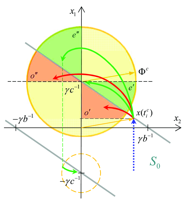
Figure 3: Slipping phases after leaving $S_{0}$.

The radius of the sphere, cf. (25), which is enclosing the ball

$$\|(x_{1}-\gamma c^{-1},x_{2},x_{3})\|<\Phi^{c}$$

is determined by $\Phi^{c}=\|x(t_{i}^{c})\|$, meaning at the point where the trajectory leaves $S_{0}$, see orange vector drawn in Fig. 3. It is evident that for any trajectory outgoing from $x(t_{i}^{c})$, the $x_{1}(t)$-value is growing as long as $x_{2}>0$, and is then falling when $x_{2}<0$. Just as obvious is that $x_{2}(t)$-value is decreasing only if $x(t)\in\mathbb{R}^{3}_{-}$, the case we are considering, and can start to increase only after zero-crossing of $x_{3}$. Furthermore, we note that even though $x(t_{i}^{c})$ lies outside the ball $\Phi^{c}$, a trajectory $x(t)$ is always attracted towards the ball $\mathcal{B}$. This is due to the fact that upon leaving $S_{0}$ the $\dot{x}_{3}<0$, being driven by the energy provided by the $(x_{1},x_{2})$ vector, while $\Gamma<0$, cf. (27). Thus, any trajectory cannot escape from the ball $\mathcal{B}$ since the system (27) is GAS.

Whether the system comes again to a stiction phase, thus producing a stick-slip cycle, depends on whether the trajectory has $x_{3}$-zero-crossing inside of the one of ‘oscillation’ regions $o^{\prime}$ or $o^{\prime\prime}$, red-colored in Fig. 3. Then, $x(t_{i+1}^{s})\in S_{0}$ and a new stick-slip cycle sets on. Note that whether a trajectory experiences an overshoot and comes into the $o^{\prime\prime}$ region depends also on the $\gamma$ and state initial values. Hence also a non-oscillatory linear sub-dynamics, i.e. all roots of the characteristic equation (10) are real, can leads to trajectories landing in the $o^{\prime\prime}$ region, see numerical examples provided in section III. On the contrary, if a trajectory $x(t)$ does not leave one of the ‘exponential’ regions $e^{\prime}$ or $e^{\prime\prime}$, green-colored in Fig. 3, then $x(t)\in\mathbb{R}^{3}\backslash S_{0}$ and there is no stick-slip cycle occurring. Also we note that if overshooting into $e^{\prime\prime}$, then there is a $x_{3}$-zero-crossing and the state attractor changes to $\bar{S}_{-}=(-\gamma c^{-1},0,0)$, cf. Fig. 3.

Following numerical examples show various asymptotic convergence scenarios with and without stick-slip cycles.

III Numerical examples

The numerical simulations of the system (1), (2) are performed by using its state-space realization (4), (5) and a standard discrete-time numerical solver of MATLAB. The sampling time is set to 0.001 sec. Note that during the slipping phases (i.e. for all times between $t_{i}^{c}$ and $t_{i+1}^{s}$) the explicit solutions of trajectories, see Appendix B, are used. During the sticking phases (i.e. for all times between $t_{i}^{s}$ and $t_{i}^{c}$), the trajectories are computed by using the equivalent system dynamics (23). This way, all trajectories are consistent and there is no solver-related issues for simulating the sign discontinuity (2). Three configurations of the system parameters $a,b,c,\gamma$. The first two parameter sets are the same as used in [4, section IV], one with three distinguished roots, and another one with one real (faster) root and two conjugate complex roots close to the origin. The third parameter set is assigned to be similar to the second one (i.e. one real and two conjugate complex roots), but with difference that the real root becomes dominant, i.e. being closer to zero. The fourth parameter set (that is similar to Example 3 in [9] is assigned so that allow for slipping phase to end in the $o^{\prime}$ region, see Fig. 3.

III-A Three distinct real roots as in [4]

Three distinct real roots $\lambda_{1,2,3}=\{-0.2,-0.5,-0.8\}$ are assigned that correspond to $a=1.5$, $b=0.66$, $c=0.08$, the relay gain is $\gamma=1$, cf. [4]. Different initial conditions given in Table I are tested.

TABLE I: Initial conditions

	con. 1	con. 2	con. 3	con. 4	con. 5	con. 6
$C_{1}$	0	12.5	0	0	12.5	6.25
$C_{2}$	0.5	0.5	1.5152	2.5	2.5	2.5
$C_{3}$	0	0	0	0	0	-4.5

Note that the boundary $\gamma/b=1.5152$ has also been used, and for one set of initial conditions (con. 1) $x(0)\in S_{0}$. The phase portraits in the $(x_{2},x_{1})$ coordinates are shown in Fig. 4. One can notice that for different initial conditions the trajectories experience one stick-slip cycle, after which converging exponentially to one of the attraction points $(\pm\gamma c^{-1},0,0)$.

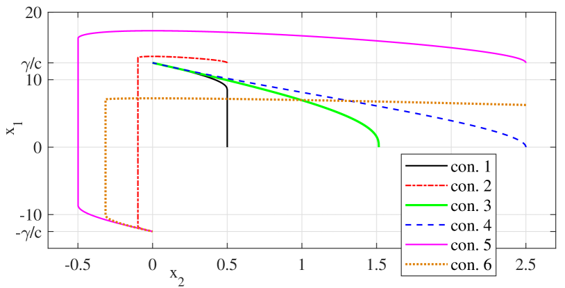
Figure 4: Phase portraits in the $(x_{2},x_{1})$ coordinates.

The corresponding time series of the $x_{2}$ state of interest (as relative displacement in case of a motion control) are shown in Fig. 5. One can recognize the largely varying period of the sticking phase, depending on $x(t^{s})$ where the trajectory entered $S_{0}$.

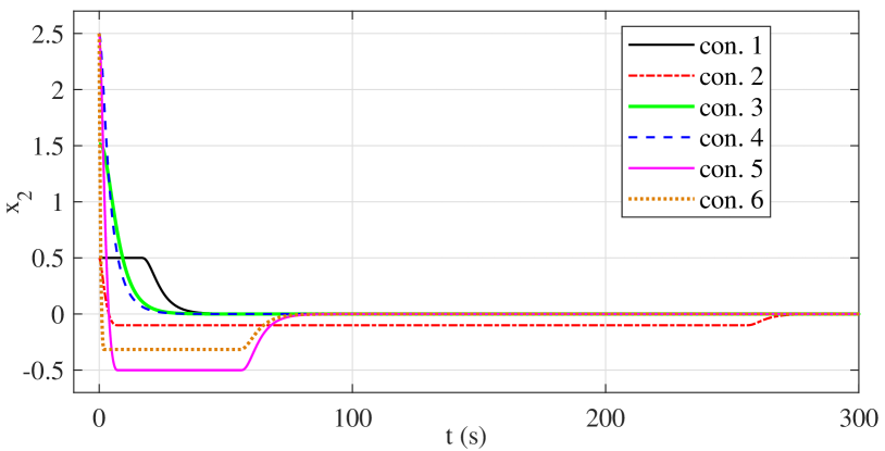
Figure 5: Time series of the $x_{2}$ state.

III-B One real and two conjugate complex roots

One real root and two conjugate complex roots $\lambda_{1,2,3}=\{-6.01,-0.19\pm j0.79\}$ are assigned that correspond to $a=6.4$, $b=3$, $c=4$, the relay gain is $\gamma=1$, cf. [4]. The pair of the conjugate complex roots corresponds to the eigenfrequency $\omega_{0}=0.8125$ and damping ratio $\delta=0.2338$, cf. Appendix B. One can recognize that the conjugate complex roots clearly dominate over the real one, since lying much closer to the origin (in the complex plane).

In addition, another configuration of the conjugate complex roots with $\omega_{0}=2$ and the same $\delta=0.2338$ was assigned. Here the real root was selected to be clearly dominating over the conjugate complex pair, thus resulting in $\{-0.2,-0.468\pm j1.94\}$. The relay gain has the same $\gamma=1$ value, while the resulted coefficients are $a=1.135$, $b=4.187$, $c=0.8$.

For both configurations of the parameters, the phase portraits are shown in Fig. 6 in the $(x_{2},x_{1})$ coordinates, and the corresponding time series of the $x_{2}$ state are shown in Fig. 7.

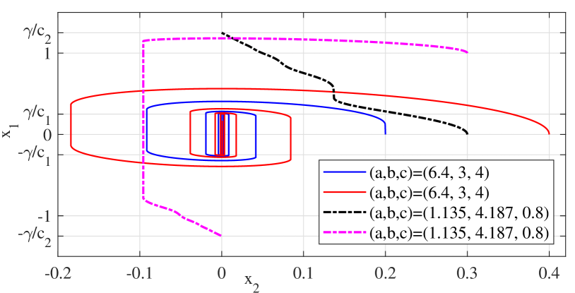
Figure 6: Phase portraits in the $(x_{2},x_{1})$ coordinates.

The first configuration of parameters is depicted by the solid lines, with two sets of the initial values $(C1,C2,C3)=\{(0,0.2,0),\>(0,0.4,0)\}$, one starting inside and other outside of $S_{0}$. The second configuration of parameters is depicted by the dash-dotted lines, with two sets of the initial values $(C1,C2,C3)=\{(0,0.3,0),\>(1,0.3,0)\}$, both starting outside of $S_{0}$.

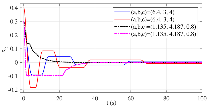
Figure 7: Time series of the $x_{2}$ state.

One can recognize that the first configuration of parameters (with the dominant conjugate complex roots) comes always to sustained stick-slip, circulating around both attraction points $(\pm\gamma c_{1}^{-1},0,0)$. On the contrary, the second configuration of parameters (with the dominant real root), although oscillatory, comes to only one stick-slip cycle, after which the trajectories are converging exponentially to one of the attraction points $(\pm\gamma c_{2}^{-1},0,0)$.

III-C Conjugate complex roots as in [9]

One real root and two conjugate complex roots $\lambda_{1,2,3}=\{-7.82,-1.09\pm j32\}$ are assigned that correspond to $a=10$, $b=1040$, $c=8000$, the relay gain is $\gamma=100$, cf. [9]. The pair of the conjugate complex roots corresponds to the eigenfrequency $\omega_{0}=32$ and damping ratio $\delta=0.034$. One can recognize that while the conjugate complex roots dominate over the real one, the otherwise highly oscillatory (with respect to $\delta$) system is largely damped by the nonlinear relay action. Thus, it is expected to come repeatedly into $S_{0}$ within $o^{\prime}$ region, in a close vicinity to $x_{2}=0$, cf. Fig. 3.

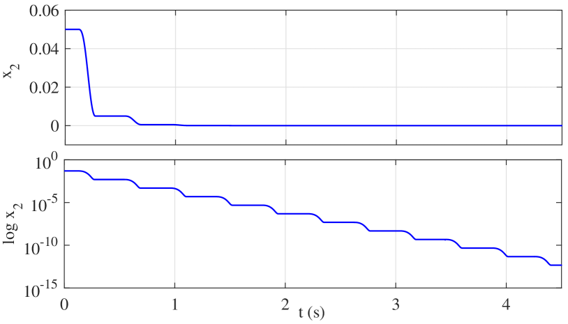
Figure 8: Time series of the $x_{2}$ state.

The time series of the $x_{2}$ state are shown in Fig. 8, once on the linear and once on the logarithmic scale.

IV Summary and discussion

In this work, a simple to follow analysis of the convergence behavior of the third-order dynamic systems which have integral feedback action and discontinuous relay disturbance was presented. The GAS property of the system was proven and the so-called stiction regime in a well-defined region of the state-space was specified and analyzed by using the sliding-mode principles. The corresponding equivalent dynamics was established and conditions for entering into and leaving from the stiction region were described. The possible scenarios of a stick-slip convergence were addressed and illustrated by the dedicated numerical examples. Following can be summarized and brought into discussion. For the real roots of characteristic polynomial of the linear subsystem, only one stick-slip cycle can appear (depending on the initial conditions) before the exponential convergence takes place towards one of the two symmetrical points of attraction. For the conjugate complex roots, the appearance of persistent stick-slip cycles can depend on whether the conjugate complex roots dominate over the real one. If such system is predominantly damped by the relay feedback action, the persistent stick-slip cycles can appear even without overshoot, see example shown in section III-C. If, otherwise, the real root dominates over the conjugate complex pair, certain low number of the stick-slip cycles (but not a persistent series) is expected before entering into the exponential convergence. However, those statements made above require a more detailed analytic analysis of both, the polynomial coefficients and the initial conditions, also taking into account the relay gain value. The latter enters directly into the particular solutions shown in the Appendix B. At large, the present work, in addition to the previously published works [3, 4, 9], should provide further insight into the problem of state feedback plus integral control behavior for the motion systems in presence of the discontinuous Coulomb friction.

Appendix

IV-A Solution of Lyapunov equation

For $Q=I$ and $A$ as given by (5), the unique solution of (9) is the $3\times 3$ symmetric matrix $P$ with the elements

$$p_{1,1} = -\frac{c(a^{2}+ac-b+c^{2})}{2c(c-ab)},$$

$$p_{1,2} = -\frac{a^{2}b+c^{2}(b+1)}{2c(c-ab)},$$

$$p_{1,3} = \frac{1}{2c},$$

$$p_{2,2} = -\frac{a(a^{2}+ac+c^{2})+c(b^{2}+b+1)}{2c(c-ab)},$$

$$p_{2,3} = -\frac{a(a+c)+c^{2}}{2c(c-ab)},$$

$$p_{3,3} = -\frac{a+c(b+1)}{2c(c-ab)}.$$

IV-B Particular solutions during the system slipping

For the system (1), (2), equivalently (4), (5), the particular solutions during slipping, i.e. for $\ddot{y}=x_{3}\neq 0$, are those of the following nonhomogeneous differential equation

$$\begin{split}\dot{x}_{3}(t)+a\,x_{3}(t)+b\,x_{2}(t)+c\,x_{1}(t)=-\Gamma,\\[1.42262pt] \qquad\forall\;\;t_{i}^{c}\leq t\,\left\{\begin{array}[]{ll}\leq t_{0}&\hbox{if }x_{3}(t_{0})=0,\\ <\infty&\hbox{if }x_{3}(t)\neq 0,\\ \end{array}\right.\end{split}$$ (27)

where the constant exogenous right-hand-side $\Gamma\equiv\gamma\,\mathrm{sign}(x_{3})$ of (27) is assigned for the particular solutions of $x\in\mathbb{R}^{3}_{-}\vee\mathbb{R}^{3}_{+}$. Next, we need to distinguish whether the corresponding characteristic polynomial (10) has all real roots or a pair of conjugate complex roots.

IV-B1 Three distinct real roots

Assume that (10) has three distinct real roots $\lambda_{1}\neq\lambda_{2}\neq\lambda_{3}$ while the dynamic system (27) is asymptotically stable, i.e. $\lambda_{1},\lambda_{2},\lambda_{3}>0$ and the inequality (6) holds for

$$a=\lambda_{1}+\lambda_{2}+\lambda_{3},\;b=\lambda_{2}\lambda_{3}+\lambda_{1}\lambda_{2}+\lambda_{1}\lambda_{3},\;c=\lambda_{1}\lambda_{2}\lambda_{3}.$$ (28)

Then, the particular solution of (27) is given by

$$x_{1}(t)=-\frac{\Gamma}{\lambda_{1}\lambda_{2}\lambda_{3}}+K_{1}e^{-\lambda_{1}t}-K_{2}e^{-\lambda_{1}t}+K_{3}e^{-\lambda_{1}t},$$ (29)

with the coefficients

$$K_{1} = \frac{\Gamma+C_{3}\lambda_{1}+C_{2}\lambda_{1}(\lambda_{2}+\lambda_{3})+C_{1}\lambda_{1}\lambda_{2}\lambda_{3}}{\lambda_{1}(\lambda_{1}-\lambda_{2})(\lambda_{1}-\lambda_{3})},$$

$$K_{2} = \frac{\Gamma+C_{3}\lambda_{2}+C_{2}\lambda_{2}(\lambda_{1}+\lambda_{3})+C_{1}\lambda_{1}\lambda_{2}\lambda_{3}}{\lambda_{2}(\lambda_{1}-\lambda_{2})(\lambda_{2}-\lambda_{3})},$$

$$K_{3} = \frac{\Gamma+C_{3}\lambda_{3}+C_{2}\lambda_{3}(\lambda_{1}+\lambda_{2})+C_{1}\lambda_{1}\lambda_{2}\lambda_{3}}{\lambda_{3}(\lambda_{1}-\lambda_{3})(\lambda_{2}-\lambda_{3})}.$$

Respectively,

$$x_{2}(t)=\dot{x}_{1}(t),\quad x_{3}(t)=\ddot{x}_{1}(t).$$ (30)

IV-B2 One real and two conjugate complex roots

Assume that (10) has one real root $\lambda_{1}$ and a pair of conjugate complex roots $\lambda_{2,3}=-\delta\omega_{0}\pm j\omega_{0}\sqrt{1-\delta^{2}}$ which are parameterized by the eigenfrequency $\omega_{0}>0$ and damping ratio $0<\delta\leq 1$. Recall that the case of the double real roots $\lambda_{2}=\lambda_{3}$ is covered by $\delta=1$. The dynamic system (27) is asymptotically stable, i.e. $\lambda_{1},\lambda_{2},\lambda_{3}>0$ and the inequality (6) holds for

$$a=2\delta\omega_{0}+\lambda_{1},\;\;b=2\delta\omega_{0}\lambda_{1}+\omega_{0}^{2},\;\;c=\lambda_{1}\omega_{0}^{2}.$$ (31)

Then, the particular solution of (27) is given by

$$x_{1}(t) = -\frac{\gamma}{\lambda_{1}\,{\omega_{0}}^{2}}$$

$$+ \frac{{\mathrm{e}}^{-\lambda_{1}\,t}\,\left(C_{1}\,\lambda_{1}\,{\omega_{0}}^{2}+2\,C_{2}\,\delta\,\lambda_{1}\,\omega_{0}+\gamma+C_{3}\,\lambda_{1}\right)}{\lambda_{1}\,\left({\lambda_{1}}^{2}-2\,\delta\,\lambda_{1}\,\omega_{0}+{\omega_{0}}^{2}\right)}$$

$$+ \frac{K_{4}{\mathrm{e}}^{-\omega_{0}\,t\,\left(\delta-\sqrt{\delta^{2}-1}\right)}}{2\,{\omega_{0}}^{2}\,\sqrt{1-\delta}\,\sqrt{-\delta-1}\,\left(\lambda_{1}-\delta\,\omega_{0}+\omega_{0}\,\sqrt{\delta^{2}-1}\right)}$$

$$+ \frac{K_{5}{\mathrm{e}}^{-\omega_{0}\,t\,\left(\delta+\sqrt{1-\delta}\,\sqrt{-\delta-1}\right)}}{2\,{\omega_{0}}^{2}\,\sqrt{1-\delta}\,\sqrt{-\delta-1}\,\left(\delta\,\omega_{0}-\lambda_{1}+\omega_{0}\,\sqrt{\delta^{2}-1}\right)},$$

with the coefficients

$$K_{4} = C_{3}\,\omega_{0}+\delta\,\gamma+\gamma\,\sqrt{\delta^{2}-1}+C_{2}\,\lambda_{1}\,\omega_{0}+C_{2}\,\delta\,{\omega_{0}}^{2}$$

$$+ C_{2}\,{\omega_{0}}^{2}\,\sqrt{\delta^{2}-1}+C_{1}\,\lambda_{1}\,{\omega_{0}}^{2}\Bigl{(}\delta+\sqrt{\delta^{2}-1}\Bigr{)},$$

$$K_{5} = C_{3}\,\omega_{0}+\delta\,\gamma-\gamma\,\sqrt{\delta^{2}-1}+C_{2}\,\lambda_{1}\,\omega_{0}+C_{2}\,\delta\,{\omega_{0}}^{2}$$

$$- C_{2}\,{\omega_{0}}^{2}\,\sqrt{\delta^{2}-1}+C_{1}\,\lambda_{1}\,{\omega_{0}}^{2}\Bigl{(}\delta-\sqrt{\delta^{2}-1}\Bigr{)}.$$

Respectively, (30) applies as well.

References

- [1] J. Alvarez, I. Orlov, and L. Acho, “An invariance principle for discontinuous dynamic systems with application to a Coulomb friction oscillator,” Journal of Dynamic Systems, Measurement, and Control, vol. 122, no. 4, pp. 687–690, 2000.
- [2] B. Armstrong, P. Dupont, and C. De Wit, “A survey of models, analysis tools and compensation methods for the control of machines with friction,” Automatica, vol. 30, pp. 1083–1138, 1994.
- [3] B. Armstrong and B. Amin, “PID control in the presence of static friction: A comparison of algebraic and describing function analysis,” Automatica, vol. 32, no. 5, pp. 679–692, 1996.
- [4] A. Bisoffi, M. Da Lio, A. Teel, and L. Zaccarian, “Global asymptotic stability of a PID control system with Coulomb friction,” IEEE Tran. on Automatic Control, vol. 63, no. 8, pp. 2654–2661, 2017.
- [5] A. Filippov, Differential Equations with Discontinuous Right-hand Sides, 1st ed. Dordrecht: Kluwer Academic Publishers, 1988.
- [6] H. Olsson and K. J. Astrom, “Friction generated limit cycles,” IEEE Tran. on Control Systems Technology, vol. 9, no. 4, pp. 629–636, 2001.
- [7] C. J. Radcliffe and S. C. Southward, “A property of stick-slip friction models which promotes limit cycle generation,” in American Control Conference, 1990, 1990, pp. 1198–1205.
- [8] M. Ruderman and M. Iwasaki, “Analysis of linear feedback position control in presence of presliding friction,” IEEJ Journal of Industry Applications, vol. 5, no. 2, pp. 61–68, 2016.
- [9] M. Ruderman, “Stick-slip and convergence of feedback-controlled systems with Coulomb friction,” Asian Journal of Control, vol. 24, no. 6, pp. 2877–2887, 2022.
- [10] M. Ruderman, Analysis and Compensation of Kinetic Friction in Robotic and Mechatronic Control Systems, 1st ed. CRC Press, 2023.
- [11] Y. Shtessel, C. Edwards, L. Fridman, and A. Levant, Sliding mode control and observation, 1st ed. Springer, 2014.
- [12] H. Khalil, Nonlinear Systems, 3rd ed. Prentice Hall, 2002.
- [13] P. Antsaklis and A. Michel, A Linear Systems Primer, 1st ed. Birkhäuser, 2007.
- [14] G. Franklin, J. Powell, and A. Emami-Naeini, Feedback control of dynamic systems, 8th ed. Pearson, 2020.
- [15] K. H. Johansson, A. Rantzer, and K. J. Åström, “Fast switches in relay feedback systems,” Automatica, vol. 35, no. 4, pp. 539–552, 1999.
- [16] K. H. Johansson, A. Barabanov, and K. J. Astrom, “Limit cycles with chattering in relay feedback systems,” IEEE Transactions on Automatic Control, vol. 47, no. 9, pp. 1414–1423, 2002.
- [17] D. Liberzon, Switching in systems and control, 1st ed. Springer, 2003.
- [18] V. Utkin, A. Poznyak, Y. V. Orlov, and A. Polyakov, Road map for sliding mode control design, 1st ed. Springer, 2020.