Generalized Hybrid Search and
Applications to Blockchain and Hash Function Security

Abstract

• In this work we first examine the hardness of solving various search problems by hybrid quantum-classical strategies, namely, by algorithms that have both quantum and classical capabilities. We then construct a hybrid quantum-classical search algorithm and analyze its success probability.

  Regarding the former, for search problems that are allowed to have multiple solutions and in which the input is sampled according to arbitrary distributions we establish their hybrid quantum-classical query complexities—i.e., given a fixed number of classical and quantum queries, determine what is the probability of solving the search task. At a technical level, our results generalize the framework for hybrid quantum-classical search algorithms recently proposed by Rosmanis [32]. Namely, for an arbitrary distribution $D$ on Boolean functions, the probability that an algorithm equipped with $\tau_{c}$ classical queries and $\tau_{q}$ quantum queries succeeds in finding a preimage of $1$ for a function sampled from $D$ is at most $\nu_{D}\cdot(2\sqrt{\tau_{c}}+2\tau_{q}+1)^{2}$, where $\nu_{D}$ captures the average (over $D$) fraction of preimages of $1$.

  As applications of our hardness results, we first revisit and generalize the formal security treatment of the Bitcoin protocol called the Bitcoin backbone [Eurocrypt 2015], to a setting where the adversary has both quantum and classical capabilities, presenting a new hybrid honest majority condition necessary for the protocol to properly operate. Secondly, we re-examine the generic security of hash functions [PKC 2016] against quantum-classical hybrid adversaries.

  Regarding our second contribution, we design a hybrid algorithm which first spends all of its classical queries and in the second stage runs a “modified Grover” in which the initial state depends on the target distribution ${D}$. We then show how to analyze its success probability for arbitrary target distributions and, importantly, its optimality for the uniform and the Bernoulli distribution cases.

1 Introduction

The query model is an elegant abstraction and is widely adopted in cryptography. A notable example is the random oracle (RO) model [7], where a hash function $f$ is modeled as a random black-box function, and all parties including the adversary can evaluate it only by issuing a query $x$ and receiving $f(x)$ in response. Numerous cryptosystems have been designed and analyzed in the random oracle model (e.g., [8, 9, 33, 23, 22]).

Quantum computing brings about a new quantum query model, where superposition queries to the hash function $f$ are permitted in the form of: $\sum_{x,y}\alpha_{x,y}|x\rangle|y\rangle\mapsto\sum_{x,y}\alpha_{x,y}|x\rangle|y\oplus f(x)\rangle$. This equips quantum adversaries with new capabilities. Indeed, some classically secure digital signature and public-key encryption schemes are broken in the quantum random oracle (QRO) model, where a quantum adversary makes superposition queries to $f$ [36]. A significant amount of effort has been devoted to address such quantum-query adversaries (cf., [6, 20, 35, 26, 2, 17, 16, 21, 18]) and often, in order to maintain security, we need to pay a considerable efficiency overhead, such as more complex constructions or larger key sizes.

The threat is alarming, but it requires running a large-scale quantum computer coherently for an extended time. The quantum devices available in the near-to-intermediate term are likely to be computationally restricted as well as expensive [31]. This reality inspires a hybrid query model, where one is granted a quota of both classical and quantum queries, a model which subsumes the classical and fully quantum query models as special cases. Establishing a trade-off between classical and quantum queries allows us to give a more accurate estimation of security and hence optimized parameter choices of a cryptosystem depending on what resources are available to a (near-term) quantum adversary.

Recently, Rosmanis studied the basic unstructured search problem in the hybrid query model [32], where given oracle function $f:X\to\{0,1\}$, one wants to find a “marked” input, i.e., $x$ with $f(x)=1$. This search problem and many variants, such as multiple or randomly chosen marked inputs, are well understood when all queries are quantum [25, 5, 37, 19, 39], where Grover’s quantum algorithm gives a quadratic speedup over classical algorithms and it is also proven optimal. Rosmanis’s work proves the hardness of searching in the domain of a function with a unique marked input $x^{*}$ in the hybrid query model. Specifically, any quantum algorithm with $\tau_{c}$ classical queries and $\tau_{q}$ quantum queries succeeds in finding $x^{*}$ with probability at most $\frac{1}{|X|}\cdot(2\sqrt{\tau_{c}}+2\tau_{q}+1)^{2}$. This hardness bound is also shown in [27] by a new recording technique tailored to the hybrid query model.

1.1 Our Contributions and Technical Overview

Success Probability Lower Bound of any Hybrid Search Algorithm.

In this work, we consider an arbitrary distribution ${D}$ on the function family $\mathcal{F}_{\textsc{}}=\{f:X\to\{0,1\}\}$, and prove a precise upper bound on the probability of finding a preimage $x$ with $f(x)=1$ when $f\leftarrow{D}$, for any algorithm $\mathcal{A}$ spending $\tau_{c}$ classical and $\tau_{q}$ quantum queries. Specifically, we show that:

$$\Pr_{f\leftarrow{D}}[f(x)=1:x\leftarrow\mathcal{A}^{{f}}]\leq\nu_{D}\cdot(2\sqrt{\tau_{c}}+2\tau_{q}+1)^{2}\,,$$

where $\nu_{D}\stackrel{{\scriptstyle\mathrm{def}}}{{=}}\sup_{\varphi:\left\lVert\varphi\right\rVert\leq 1}\left(\mathbb{E}_{f\leftarrow{D}}\left\lVert\left(\sum_{x:f(x)=1}|x\rangle\langle x|\right)\varphi\right\rVert^{2}\right)$ captures the average fraction of preimages of $1$, and is solely determined by the distribution ${D}$.

With our generalized bound, deriving hardness bounds for specific distributions becomes convenient. All we need is to analyze $\nu_{D}$, and this usually can be done by simple combinatorial arguments. For instance, let ${D}$ be the uniform distribution over functions with exactly one marked input. Then we can observe that $\nu_{D}=\Pr_{f\leftarrow{D}}[f(x)=1]={1}/{|X|}$ for an arbitrary $x$, which recovers the result of Rosmanis [32]. The hardness of searching a function with $w>1$ marked items can be similarly derived.

We further demonstrate our result on another distribution ${D}_{\eta}$, where each input is marked according to a Bernoulli trial. Namely, for every $x\in X$, we set $f(x)=1$ with probability $\eta$ independently. By determining $\nu_{D}$ in this case, we derive the hardness of search when the function is drawn from ${D}_{\eta}$. This search problem under ${D}_{\eta}$, which we call Bernoulli Search, is particularly useful in several cryptographic applications. Firstly, we can prove generic security bounds for hash function properties, such as preimage-resistance, second-preimage resistance and their multi-target extensions, against hybrid quantum-classical adversaries. This follows by adapting the reductions in [28], where the hash properties are connected to the Bernoulli Search problem in the fully quantum query setting and then plugging in our hybrid hardness bound of Bernoulli Search. In another application, Bernoulli Search was shown to dictate the security of proofs of work (PoWs) and security properties of Bitcoin-like blockchains in the random oracle model (with fully quantum queries) [14]. This allows us to identify a new honest-majority condition under which the security of Bitcoin blockchain holds against hybrid adversaries with classical and quantum queries.

At a technical level, the proof of our hardness bound follows the overall strategy of [32]. As in the standard optimality proof of Grover’s algorithm [5], one would consider running an adversary’s algorithm with respect to the input function $f\leftarrow{D}$ or a constant-0 function. Then one argues that each query diverges the states in these two cases, which is called a progress measure, by a small amount. On the other hand, in order to find a marked input in $f$, the final states need to differ significantly. Therefore, sufficiently many queries are necessary for the cumulative progress to grow adequately.

Now, when classical queries are mixed with quantum queries, the quantum states would collapse after each classical query and it becomes unclear how to measure the progress. To address this, Rosmanis considers instead an intermediate oracle named pseudo-classical. Namely, consider a quantum query with the output register initialized in $|0\rangle$: $\sum_{x}\alpha_{x}|x\rangle|0\rangle\mapsto\sum_{x}\alpha_{x}|x\rangle|f(x)\rangle$. We can then view a classical query as the result of measuring the input register that collapses to $x$ and receiving $f(x)$, whereas a pseudo-classical oracle measures the output register, resulting in one of two possible outcomes: $\sum_{x:f(x)=0}\alpha_{x}|x\rangle|0\rangle$ (denoted as the 0-outcome branch) or $\sum_{x:f(x)=1}\alpha_{x}|x\rangle|1\rangle$ (denoted as the 1-outcome branch). With this change, one instead tracks the progress between the 0-outcome branch in case of $f\leftarrow{D}$ and the state in case of the constant-0 function (which always stays in the 0-outcome branch). The algorithm fails if its state stays in the 0-outcome branch and is close to the state in the constant-0 case. A key ingredient in our proof is to deliberately separate the evolution of various objects on an individual function and what characteristics of the distribution ${D}$ influence the evolution and in what way. This enables us to obtain a clean and concise lower bound for the generalized hybrid search problem.

Hybrid Search Algorithms: Design and Analysis.

In the second part of our work we construct a hybrid algorithm for the search problem for an arbitrary distribution ${D}$ and show that in several interesting cases (e.g., Bernoulli) algorithm is optimal, hence leading to tight query complexity in the hybrid model. Inspired by our hardness analysis, our algorithm proceeds in a two-stage fashion:

• The first stage is purely classical. We query the $\tau_{c}$ inputs $x$ that are the most likely to be assigned the value 1 under ${D}$. More precisely, for any $x$ in the input domain, let the function $\omega(x)=\sum_{f}D(f)\cdot f(x)$, which can be viewed as the (unnormalized) probability that $f(x)=1$ with $f$ drawn from ${D}$. Let $S$ be the set of inputs whose $\omega(x)$ values are the $\tau_{c}$-highest (ties are broken arbitrarily). Then algorithm queries all the points $x\in S$. If none of them give a solution, we move on to the second stage.

• The second stage is fully quantum. We run a modified Grover’s algorithm $\mathcal{A}$ which is tailored to the prior knowledge on the distribution ${D}$. Instead of starting from an equal superposition of all points in the search space as in the standard Grover’s search algorithm, we construct an initial state in which the amplitude of each point is proportional to $\omega(x)$. Then, for each of the $\tau_{q}$ quantum queries, two reflection operators are applied to rotate the initial state towards a target state encoding the solutions. We give a comprehensive analysis and derive a clean lower bound for the success probability of $\mathcal{A}$ on the distribution ${D}$, which amounts to $\tau_{q}^{2}\cdot\frac{\sum_{x}\omega^{2}(x)}{\sum_{x}\omega(x)}$. To be more clear, for the algorithm in the second stage, we define an induced distribution $\tilde{}{D}$ by restricting and (re-normalizing) ${D}$ to functions $f$ satisfying $f(x)=0$ for all $x\in S$. Then we invoke the quantum algorithm $\mathcal{A}$ on $\tilde{}{D}$ in a modular way.

Note that the hybrid algorithm needs to compute the values $\omega(x)$ from the description of the target distribution ${D}$ and during the quantum procedure, the algorithm will implement a unitary dependent on the $\omega(x)$ values, hence the algorithm needs not be time efficient.

We can show that the success probability of the hybrid algorithm is at least the average of the success probabilities of the classical stage and of the quantum stage. In some special cases, such as the Bernoulli distribution, both the classical probability (i.e., at least one success in $\tau_{c}$ Bernoulli trials) and the weights $w(x)$ (hence the quantum success probability) are easy to derive. We can show that the hybrid algorithm gives matching lower bounds to the hardness bounds that we proved in the first part of our work.

We believe that the hybrid query model is both of theoretical and practical importance. Since near-term quantum computers are limited and expensive, it is to the interest of a party to supplement it with massive classical computational power. This also reflects the fact that those parties who have early access to quantum computers (e.g., big companies and government agencies) largely coincide with those who are capable of employing classical clusters and supercomputers. Next, we discuss some future directions.

One immediate question is to study other problems in the hybrid query model. The work of [27] also proves the hardness of the collision problem by their generalized recording technique in the hybrid query model. It would be useful to further develop techniques and establish more query complexity results.

Our applications to hash functions and Bitcoin blockchains can be seen as analyzing cryptographic constructions in the QRO model against hybrid adversaries. Many block ciphers rely on a different model, known as the ideal cipher model. As a simple example, the Even-Mansour cipher encrypts by $E_{k}:m\mapsto\sigma(k\oplus m)\oplus k$, where $\sigma$ is a random permutation given as an oracle. As it turns out, this classically secure cipher is completely broken when quantum queries are allowed to both $E_{k}$ and $\sigma$ [30]. Since the secret key $k$ is managed by honest users, it is debatable whether superposition access to $E_{k}$ is realistic. There has been progress in re-establishing the cipher’s security under a partially quantum adversary with quantum access to $\sigma$ but classical access to $E_{k}$ [29, 1]. The hybrid query model we consider in this work suggests further relaxing the queries to $\sigma$ to be a hybrid of classical and quantum ones, and it would be valuable to re-examine the security of such schemes in the ideal cipher model.

Querying an oracle also appears more broadly in many other cryptographic scenarios. Security definitions often give some algorithm as an oracle to the adversary, such as an encryption oracle in the chosen-plaintext-attack (CPA) game and a signing oracle in formalizing unforgeability of digital signatures. There has been a considerable effort of settling appropriate definitions and constructions (e.g., quantum-accessible pseudorandom functions, encryption and signatures) when quantum adversaries are granted superposition queries to these oracles (cf. [10, 38, 3, 40, 13]). Extending such efforts to the hybrid-adversary landscape would offer fine-grained security assessments of post-quantum cryptosystems. Finally, in the context of complexity theory, the study of hybrid algorithms is further motivated by related models focusing on the interplay between classical computation and near-future quantum devices [11] and between circuit depth and quantum queries [34, 15, 12].

Updates from previous version (https://eprint.iacr.org/archive/2023/798/20230703:172204) of this paper

: We have added the design and analysis of fully quantum as well as hybrid algorithms for distributional search, and have shown the optimality for special cases. This supplements the hardness results in the previous version.

1.2 Organization of the paper

The rest of the paper is organized as follows. The generalized search problem, which we call Distributional Search, is defined in Section 2.1, and its hybrid quantum-classical hardness is proven in Section 2.2 and Section 2.4. Section 2.3 describes two case studies—Grover-like Search and Bernoulli Search and Section 3 demonstrates applications of the Bernoulli Search results, where we show the generic security of hash functions (Sections 3.1) and the security of the Bitcoin blockchain against hybrid adversaries (Sections 3.2). In Section 4 we construct a quantum search algorithm and establish its probability of success for any target distribution. Section 5 describes our proposed hybrid search algorithm, as well as the approach for the analysis of general distributions, and also shows the optimality of the algorithm for particular distributions.

2 Distributional Search with Hybrid Strategies

2.1 The Distributional Search Problem

The underlying problem we consider is the search for a preimage of $1$ of an arbitrarily distributed black-box boolean function.

Distributional Search Problem (Dist-Search) Let ${D}$ be an arbitrary distribution supported on the function family $\mathcal{F}:=\left\{f:X\to\{0,1\}\right\}$. Given: Black-box access to function $f$ drawn from distribution $D$. Goal: Find $x$ such that $f(x)=1$ if there exists such an $x$.

It is not surprising that the hardness of the problem is crucially influenced by the number of preimages of $1$ on average under ${D}$; however, what is interesting about our study is that we can show a clean quantitative relation. Let $f:X\to\{0,1\}$ be an arbitrary function. Define the projector on the space spanned by preimages of $1$:

$$\pi_{f}\stackrel{{\scriptstyle\mathrm{def}}}{{=}}\sum_{x:f(x)=1}|x\rangle\langle x|\,.$$

Denote $\pi_{f}^{\perp}\stackrel{{\scriptstyle\mathrm{def}}}{{=}}\mathds{1}-\pi_{f}$, and let ${D}$ be a distribution on $\mathcal{F}$. We define the value that captures the average fraction of preimages of $1$ as:

Definition 1 ($\nu_{D}$).

The average fraction of preimages of $1$ is defined as:

$$\nu_{D}\stackrel{{\scriptstyle\mathrm{def}}}{{=}}\sup_{\varphi:\left\lVert\varphi\right\rVert\leq 1}\left(\mathbb{E}_{f\leftarrow{D}}\left\lVert\pi_{f}\varphi\right\rVert^{2}\right)$$ (1)

where $\left\lVert\varphi\right\rVert$ denotes the Euclidean norm of the quantum state $\varphi$.

In this paper, we are able to establish the following bound for the success probability of solving Dist-Search, which constitutes one of our main results:

Theorem 2.1 (Hardness of Dist-Search).

For any algorithm $\mathcal{A}$ making up to $\tau_{c}$ classical queries and $\tau_{q}$ quantum queries, it holds that:

$${\mathsf{Succ}}_{\mathcal{A},{D}}:=\Pr_{f\leftarrow{D}}[f(x)=1:x\leftarrow\mathcal{A}^{{f}}]\leq\nu_{D}\cdot(2\sqrt{\tau_{c}}+2\tau_{q}+1)^{2}\,.$$

Next, we turn to proving the above result.

2.2 Hardness of Dist-Search

2.2.1 Preliminaries and Overview

We first formally describe an oracle function for the case of quantum and pseudo-classical queries.

Definition 2 (Query Operators).

We define the following operators, which describe the actions of quantum and pseudo-classical oracles for a hybrid algorithm given a boolean function $f$.

• A pseudo-classical oracle is described by

  $$P_{f,b}\stackrel{{\scriptstyle\mathrm{def}}}{{=}}\sum_{x:f(x)=b}|x\rangle\langle x|\otimes\mathds{1}\otimes|b\rangle$$

• A quantum oracle is described by

  $$Q_{f}\stackrel{{\scriptstyle\mathrm{def}}}{{=}}\sum_{x,b}|x\rangle\langle x|\otimes\mathds{1}\otimes|b\oplus f(x)\rangle\langle b|$$

We denote $\Pi_{f}\stackrel{{\scriptstyle\mathrm{def}}}{{=}}\pi_{f}\otimes\mathds{1}$ ($\mathds{1}$ operates on the output and ancilla registers) and $\Pi_{f}^{\perp}\stackrel{{\scriptstyle\mathrm{def}}}{{=}}\mathds{1}-\Pi_{f}$ ($\mathds{1}$ operates on the entire system). Then on a pseudo-classical query, the two operators $P_{f,0}=\Pi_{f}^{\perp}\otimes|0\rangle$ and $P_{f,1}=\Pi_{f}\otimes|1\rangle$ correspond to the two possible measurement outcomes. It is more convenient to answer quantum queries by the corresponding phase oracle:

$$Q_{f}\stackrel{{\scriptstyle\mathrm{def}}}{{=}}\mathds{1}-2\Pi_{f}\,.$$

This can be seen as setting the output register of the standard oracle in $|-\rangle$, and as a result, a quantum query flips the signs of the $1$-preimages.

When running a hybrid query algorithm with $f$, we will keep track of the (sub-normalized) pure state $\psi_{f}^{(t)}$, which denotes the state of the algorithm on input $f$ after $t$ queries in the situation where every pseudo-classical query measures $0$ (we will call this the $0$-branch of $\mathcal{A}^{f}$). Namely, consider an arbitrary algorithm with at most $\tau$ queries ($\tau_{q}$ quantum and $\tau_{c}$ pseudo-classical) specified by a sequence of unitary operators $(U^{(0)},U^{(1)},\ldots,U^{(\tau)})$. Let $T_{c}=\{t:\text{$t$-th query is pseudo-classical}\}$ and $T_{q}=\{t:\text{$t$-th query is quantum}\}$. Then $\psi_{f}^{(t)}$ is defined recursively by

$$\psi_{f}^{(t)}\stackrel{{\scriptstyle\mathrm{def}}}{{=}}\begin{cases}U^{(t)}P_{f,0}\psi_{f}^{(t-1)},&\text{if }t\in T_{c}\,;\\ U^{(t)}Q_{f}\psi_{f}^{(t-1)}&\text{if }t\in T_{q}\,.\end{cases}$$ (2)

From this definition, the projection of $\psi_{f}^{(t)}$ under $\Pi_{f}^{\perp}$ characterizes the event that an algorithm fails to find a $1$-preimage.

Lemma 1.

For any algorithm $\mathcal{A}$, the failure probability of finding a $1$-preimage of $f$ after $t$ queries is

$$\delta_{f}^{(t)}=\Pr[f(x)\neq 1:x\leftarrow\mathcal{A}^{f}]\geq\left\lVert\Pi_{f}^{\perp}\psi_{f}^{(t)}\right\rVert^{2}\,.$$

Hence, the failure probability with respect to distribution ${D}$ satisfies

$$\delta_{D}^{(t)}=\mathbb{E}_{f\leftarrow D}\delta_{f}^{(t)}\geq\mathbb{E}_{f\leftarrow{D}}\left\lVert\Pi_{f}^{\perp}\psi_{f}^{(t)}\right\rVert^{2}\,.$$

Thus, our goal becomes lower-bounding $\left\lVert\Pi_{f}^{\perp}\psi_{f}^{(t)}\right\rVert$. To do this, we consider running the same algorithm, but with a null function:

$$f_{\emptyset}:x\mapsto 0,\forall x\in X\,.$$

In this case, a quantum query is equivalent to applying identity (denoted $Q_{\emptyset}\stackrel{{\scriptstyle\mathrm{def}}}{{=}}\mathds{1}$), and a pseudo-classical query does not tamper the input state either, but just appends $|0\rangle$. To be precise, we define

$$P_{\emptyset,0}\stackrel{{\scriptstyle\mathrm{def}}}{{=}}\mathds{1}\otimes|0\rangle\,,$$

and at each step $t\geq 0$, the state of the algorithm denoted by $\phi^{(t)}$ can be described as:

$$\phi^{(t)}=\begin{cases}U^{(t)}P_{\emptyset,0}\phi^{(t-1)},&\text{if }t\in T_{c}\,;\\ U^{(t)}\phi^{(t-1)}&\text{if }t\in T_{q}\,.\end{cases}$$

Without loss of generality we assume initially $\psi_{f}^{(0)}=\phi^{(0)}=|0\rangle$, and hence $\left\lVert\Pi_{f}^{\perp}\psi_{f}^{(0)}\right\rVert=\left\lVert\Pi_{f}^{\perp}\phi^{(0)}\right\rVert=1$. In order to succeed, algorithm $\mathcal{A}^{f}$ needs to move $\psi_{f}^{(t)}$ away from the kernel of $\Pi_{f}^{\perp}$ or reduce its norm. This motivates defining the progress measures below.

Definition 3 (Progress Measures $(A^{(t)},B^{(t)})$).

For any function $f$ and $t\geq 0$, define

$$A_{f}^{(t)}\stackrel{{\scriptstyle\mathrm{def}}}{{=}}\left|\langle\phi^{(t)},\psi_{f}^{(t)}\rangle\right|^{2}\,,\quad B_{f}^{(t)}\stackrel{{\scriptstyle\mathrm{def}}}{{=}}\left\|\psi_{f}^{(t)}\right\|^{2}-\left|\langle\phi^{(t)},\psi_{f}^{(t)}\rangle\right|^{2}\,.$$

Given a distribution ${D}$ on $\mathcal{F}$, define the expected progress measures by

$$A_{D}^{(t)}\stackrel{{\scriptstyle\mathrm{def}}}{{=}}\mathbb{E}_{f\leftarrow{D}}\left(A_{f}^{(t)}\right)\,,\quad B_{D}^{(t)}\stackrel{{\scriptstyle\mathrm{def}}}{{=}}\mathbb{E}_{f\leftarrow{D}}\left(B_{f}^{(t)}\right)\,.$$

Notice that

$$A_{f}^{(t)}+B_{f}^{(t)}=\left\lVert\psi_{f}^{(t)}\right\rVert^{2},\quad A_{f}^{(0)}=1,\quad B_{f}^{(0)}=0\,.$$

We will show that $A_{D}^{(t)}-B_{D}^{(t)}$ essentially lower bounds the failure probability $\delta_{D}^{(t)}$ (Lemma 5). Hence, an algorithm’s objective would be to reduce $A_{D}^{(t)}$ and increase $B_{D}^{(t)}$. However, we can limit how much change can occur after $\tau$ queries (Proposition 1). This is by carefully analyzing the effect of each quantum or pseudo-classical query (Lemmas 7 and 8). Roughly speaking,

• A quantum query reduces $A_{D}^{(t)}$ by at most $4\sqrt{\nu_{D}\cdot B_{D}^{(t)}}$ and increases $B_{D}^{(t)}$ by the same amount (as a quantum query does not affect $\left\lVert\psi_{f}^{(t)}\right\rVert^{2}$), and

• A pseudo-classical query increases $B_{D}^{(t)}$ by at most $\nu_{D}$, while a part $z^{(t)}$ of $B_{D}^{(t)}$ can also be spent to decrease $A_{D}^{(t)}$ by $\sqrt{\nu_{D}\cdot z^{(t)}}$.

$\pi_{f}$	$\sum_{x:f(x)=1}|x\rangle\langle x|$
$\Pi_{f}$	$\pi_{f}\otimes\mathds{1}$ ($\mathds{1}$ on ancilla registers)
$\delta_{f}$	$\Pr[f(x)\neq 1:x\leftarrow\mathcal{A}^{f}]$ (Failure probability with $f$)
$\delta_{D}$	$\mathbb{E}_{D}\delta_{f}$ (Failure probability with $f\leftarrow{D}$)
$\phi^{(0)}=\psi^{(0)}$	Initial state
$\phi^{(t)}$	State after $t$-th query in $\mathcal{A}^{f_{\emptyset}}$
$\psi_{f}^{(t)}$	State on the 0-branch after $t$-th query in $\mathcal{A}^{f}$
$Q_{f}$	$\mathds{1}-2\Pi_{f}$ (quantum oracle of $f$)
$Q_{\emptyset}$	$\mathds{1}$ (quantum oracle of $f_{\emptyset}$)
$P_{f,0}$	$\Pi_{f}^{\perp}\otimes|0\rangle$ (pseudo-classical oracle of $f$)
$P_{f,1}$	$\Pi_{f}\otimes|1\rangle$ (pseudo-classical oracle of $f$)
$P_{\emptyset,0}$	$\mathds{1}\otimes|0\rangle$ (pseudo-classical oracle of $f_{\emptyset}$)
$\gamma_{f}^{(t)}$	$\left\lVert\Pi_{f}\phi^{(t)}\right\rVert^{2}$
$\gamma^{(t)}$	$\mathbb{E}_{D}(\gamma_{f}^{(t)})$

Table 1: Summary of variables and quantities used in our Dist-Search analysis.

2.2.2 Proof of Theorem 2.1

First off, we state the Cauchy-Schwarz inequality for random variables and derive a lemma that is useful in several places.

Lemma 2 (Cauchy-Schwarz).

For any random variables $X$, $Y$, it holds that:

$$\left|\mathbb{E}{[XY]}\right|^{2}\leq\mathbb{E}{[X^{2}]}\cdot\mathbb{E}{[Y^{2}]}.$$

As a direct consequence of the Cauchy-Schwarz inequality, we have the following useful corollary.

Corollary 1.

Let $Z$ be a discrete random variable, and $g(Z)$ and $h(Z)$ be two non-negative functions. Then it holds that:

$$\mathbb{E}_{Z}\left(\sqrt{g(Z)\cdot h(Z)}\right)\leq\sqrt{\mathbb{E}_{Z}g(Z)\cdot\mathbb{E}_{Z}h(Z)}\,.$$

It will be helpful to consider a two-dimensional plane in our analysis, which we now define explicitly.

Definition 4 (Useful 2-D Plane).

For $t\geq 0$, let

$$\phi_{f}^{(t)}\stackrel{{\scriptstyle\mathrm{def}}}{{=}}\frac{\Pi_{f}\phi^{(t)}}{\left\lVert\Pi_{f}\phi^{(t)}\right\rVert}=\Pi_{f}\phi^{(t)}/\sqrt{\gamma_{f}^{(t)}}\,,\qquad\phi_{f}^{(t)\perp}\stackrel{{\scriptstyle\mathrm{def}}}{{=}}\frac{\Pi_{f}^{\perp}\phi^{(t)}}{\left\lVert\Pi_{f}^{\perp}\phi^{(t)}\right\rVert}=\Pi_{f}^{\perp}\phi^{(t)}/\sqrt{1-\gamma_{f}^{(t)}}\,$$

be the normalized vectors resulting of projecting $\phi$ on the orthogonal subspaces spanned by $1$ and $0$ preimages of $f$, respectively, and let $\Phi^{(t)}$ be the $2$-dimensional plane spanned by $\{\phi_{f}^{(t)},\phi_{f}^{(t)\perp}\}$. Then $\phi^{(t)\perp}$ is identified as the normalized state perpendicular to $\phi^{(t)}$ in $\Phi^{(t)}$, i.e.,

$$\phi^{(t)\perp}\stackrel{{\scriptstyle\mathrm{def}}}{{=}}\phi_{f}^{(t)}\sqrt{1-\gamma_{f}^{(t)}}-\phi_{f}^{(t)\perp}\sqrt{\gamma_{f}^{(t)}}\,.$$

It is useful to decompose $\psi_{f}^{(t)}$ with respect to $\Phi^{(t)}$:

Lemma 3 (Decomposition of $\psi_{f}^{(t)}$ wrt $\Phi^{(t)}$).

Let $a$ and $b$ be projecting $\psi_{f}^{(t)}$ on the plane $\Phi^{(t)}$ and then decomposing it under basis $\{\phi^{(t)},\phi^{(t)\perp}\}$, and let $c$ be the remaining component of $\psi_{f}^{(t)}$ orthogonal to $\Phi^{(t)}$, i.e., $c\perp\Phi^{(t)}$. Then $\psi_{f}^{(t)}$ can be expressed as $\psi_{f}^{(t)}=a+b+c$ with

$$a=\phi^{(t)}\sqrt{A_{f}^{(t)}}\,,\qquad b=\omega\sqrt{B_{f}^{(t)}-\left\lVert c\right\rVert^{2}}\cdot\phi^{(t)\perp}\,,$$

where $\omega$ is a complex phase (i.e., $|\omega|=1$) of the vector $\psi_{f}^{(t)}-\langle\psi_{f}^{(t)},\phi_{f}^{(t)}\rangle\cdot\phi^{(t)}-c$. As a result,

$$\Pi_{f}^{\perp}\psi_{f}^{(t)}=\phi_{f}^{(t)\perp}\left(\sqrt{1-\gamma_{f}^{(t)}}\sqrt{A_{f}^{(t)}}-\sqrt{\gamma_{f}^{(t)}}\cdot\omega\sqrt{B_{f}^{(t)}-\left\lVert c\right\rVert^{2}}\right)+c_{f}^{\perp}\,,$$

with $c_{f}^{\perp}:=\Pi_{f}^{\perp}c$.

Intuitively, for the next result, the goal is to relate the failure probability with the progress measures $A$ and $B$. To do so, we will first relate the failure probability with the norm of the non-solution component. By decomposing this norm in terms of the two progress measures A and B and an orthogonal component which can be removed, we can determine a lower bound on the failure probability as a function of the two progress measure after each performed query.

Lemma 4.

For any fixed $f$ and $t\geq 0$,

$$\delta_{f}^{(t)}\geq A_{f}^{(t)}-\gamma_{f}^{(t)}-2\sqrt{\gamma_{f}^{(t)}\cdot B_{f}^{(t)}}\,.$$

Proof.

For convenience, we omit writing the superscript $(t)$ in this proof. We first show that $\left\lVert\pi_{f}^{\perp}\psi_{f}\right\rVert\geq\sqrt{(1-\gamma_{f})A_{f}}-\sqrt{\gamma_{f}B_{f}}$. By Lemma 3, we have that

$$\Pi_{f}^{\perp}\psi_{f}={\phi_{f}^{\perp}}\left(\sqrt{1-\gamma_{f}}\sqrt{A_{f}}-\sqrt{\gamma_{f}}\cdot\omega\sqrt{B_{f}-\left\lVert c\right\rVert^{2}}\right)+c_{f}^{\perp}\,,$$

with $c_{f}^{\perp}:=\pi_{f}^{\perp}c$. Since $c\perp\Phi$, it follows that

$$\langle\phi_{f}^{\perp},c_{f}^{\perp}\rangle=\langle\phi_{f}^{\perp},\Pi_{f}^{\perp}c\rangle=\langle\Pi_{f}^{\perp}\phi_{f}^{\perp},c\rangle=\langle\phi_{f}^{\perp},c\rangle=0\,.$$

We can then obtain:

$$\left\lVert\Pi_{f}^{\perp}\psi_{f}\right\rVert=\left|\sqrt{1-\gamma_{f}}\cdot\sqrt{A_{f}}-\sqrt{\gamma_{f}}\cdot\omega\sqrt{B_{f}-\left\lVert c\right\rVert^{2}}\right|+\left\lVert c_{f}^{\perp}\right\rVert$$

Hence by choosing $c=0,\omega=1$, we get that

$$\left\lVert\Pi_{f}^{\perp}\psi_{f}\right\rVert\geq\sqrt{(1-\gamma_{f})A_{f}}-\sqrt{\gamma_{f}B_{f}}\,.$$

Therefore we can lower bound the failure probability

$$\delta_{f} \geq\left\lVert\pi_{f}^{\perp}\psi_{f}\right\rVert^{2}$$

$$\geq(1-\gamma_{f})A_{f}-2\sqrt{(1-\gamma_{f})\gamma_{f}B_{f}}$$

$$\geq A_{f}-\gamma_{f}-2\sqrt{\gamma_{f}B_{f}}\qquad\text{($A_{f},\gamma_{f}\leq 1$)}$$

∎

Taking the expectation over ${D}$, we can express the failure probability with respect to the distribution.

Lemma 5.

For any distribution ${D}$ and $t\geq 0$,

$$\delta_{D}^{(t)}\geq A^{(t)}-\gamma^{(t)}-2\sqrt{\gamma^{(t)}\cdot B^{(t)}}\,.$$

Proof.

$$\delta_{D}^{(t)} =\mathbb{E}_{f\leftarrow{D}}(\delta_{f}^{(t)})$$

$$\geq\mathbb{E}_{D}(A_{f}^{(t)})-\mathbb{E}_{D}(\gamma_{f}^{(t)})-2\mathbb{E}_{D}\sqrt{\gamma_{f}^{(t)}\cdot B_{f}^{(t)}}\qquad\text{(Linearity of expectation)}$$

$$\geq A^{(t)}-\gamma^{(t)}-2\sqrt{\mathbb{E}_{D}(\gamma_{f}^{(t)})\cdot\mathbb{E}_{D}(B_{f}^{(t)})}\qquad\text{(\lx@cref{creftype~refnum}{lemma:expproduct})}$$

$$=A^{(t)}-\gamma^{(t)}-2\sqrt{\gamma^{(t)}\cdot B^{(t)}}$$

∎

We can also relate $\gamma^{(t)}$ to the value $\nu_{D}$ determined by the distribution ${D}$:

Lemma 6.

For any $t\geq 0$ and any distribution ${D}$, we have: $\gamma^{(t)}\leq\nu_{D}$.

Proof.

$$\begin{split}\gamma^{(t)}&:=\mathbb{E}_{f\leftarrow{D}}\left\lVert\Pi_{f}\phi^{(t)}\right\rVert^{2}=\mathbb{E}_{f\leftarrow{D}}\left\lVert(\pi_{f}\otimes\mathds{1})\phi^{(t)}\right\rVert^{2}\\ \end{split}$$

We write $\phi^{(t)}=\sum_{i}\alpha_{i}|u_{i}\rangle\otimes|v_{i}\rangle$ under the Schmidt decomposition, where $\alpha_{i}\geq 0$ such that $\sum_{i}\alpha_{i}^{2}=1$ are the Schmidt coefficients, and $\{|u_{i}\rangle\}$ are orthonormal states on the system of the input register and $\{|v_{i}\rangle\}$ are orthonormal states on the system of output and ancilla registers.

Then we can rewrite $\gamma^{(t)}$ as

$$\begin{split}\gamma^{(t)}&:=\mathbb{E}_{f\leftarrow{D}}\left\lVert(\pi_{f}\otimes\mathds{1})\phi^{(t)}\right\rVert^{2}=\mathbb{E}_{f\leftarrow{D}}\left\lVert(\pi_{f}\otimes\mathds{1})\left(\sum_{i}\alpha_{i}|u_{i}\rangle\otimes|v_{i}\rangle\right)\right\rVert^{2}\\ &=\mathbb{E}_{f\leftarrow{D}}\left\lVert\sum_{i}\alpha_{i}(\pi_{f}|u_{i}\rangle)\otimes|v_{i}\rangle\right\rVert^{2}\\ &=\mathbb{E}_{f\leftarrow{D}}\sum_{i}\alpha_{i}^{2}\left\lVert(\pi_{f}|u_{i}\rangle)\otimes|v_{i}\rangle\right\rVert^{2}\qquad\text{($|v_{i}\rangle$ are orthogonal)}\\ &=\mathbb{E}_{f\leftarrow{D}}\sum_{i}\alpha_{i}^{2}\left\lVert\pi_{f}|u_{i}\rangle\right\rVert^{2}\cdot\left\lVert|v_{i}\rangle\right\rVert^{2}\qquad\text{($\left\lVert a\otimes b\right\rVert=\left\lVert a\right\rVert\cdot\left\lVert b\right\rVert$)}\\ &=\mathbb{E}_{f\leftarrow{D}}\sum_{i}\alpha_{i}^{2}\left\lVert\pi_{f}|u_{i}\rangle\right\rVert^{2}\\ &=\sum_{i}\alpha_{i}^{2}\mathbb{E}_{f\leftarrow{D}}\left\lVert\pi_{f}|u_{i}\rangle\right\rVert^{2}\\ &\leq\sum_{i}\alpha_{i}^{2}\nu_{D}\qquad\text{(definition of $\nu_{D}$)}\\ &=\nu_{D}\sum_{i}\alpha_{i}^{2}=\nu_{D}\end{split}$$

∎

Proposition 1 (Bounding Progress Measures).

After $\tau=\tau_{c}+\tau_{q}$ queries,

$$A^{(\tau)}\geq 1-4\nu_{D}\cdot(\sqrt{\tau_{c}}+\tau_{q})^{2}\,,\quad B^{(\tau)}\leq\nu_{D}\cdot(\sqrt{\tau_{c}}+2\tau_{q})^{2}\,.$$

Proving Proposition 1 is the most involved step technically speaking. We present the details separately in Section 2.4 and here we apply it to prove Theorem 2.1.

Proof of Theorem 2.1.

Assuming the bounds above on the two progress measures, we obtain that:

$$\delta^{(\tau)} \geq 1-4\gamma^{(\tau)}\cdot(\sqrt{\tau_{c}}+\tau_{q})^{2}-\gamma^{(\tau)}-2\gamma^{(t)}\cdot(\sqrt{\tau_{c}}+2\tau_{q})\qquad\text{(\lx@cref{creftype~refnum}{prop:progressbound})}$$

$$=1-\gamma^{(\tau)}\cdot(4(\sqrt{\tau_{c}}+\tau_{q})+2\sqrt{\tau_{c}}+4\tau_{q}+1)$$

$$\geq 1-\gamma^{(\tau)}\cdot(2(\sqrt{\tau_{c}}+\tau_{q})+1)^{2}\qquad\text{($\tau_{c}\geq 0$)}$$

$$\geq 1-\nu_{D}\cdot(2\sqrt{\tau_{c}}+2\tau_{q}+1)^{2}\qquad\text{($\gamma^{(\tau)}\leq\nu_{D}$~{}\lx@cref{creftype~refnum}{lemma:gammavssolnl})}$$

Therefore,

$${\mathsf{Succ}}_{\mathcal{A},{D}}\leq 1-\delta^{(\tau)}\leq\nu_{D}\cdot(2\sqrt{\tau_{c}}+2\tau_{q}+1)^{2}\,.$$

∎

2.3 Case Studies

In this section, we will apply our main result to two common function distributions. As a common ingredient, it will be helpful to consider the following indicator random variable:

$$\mathds{1}_{x}^{f}\stackrel{{\scriptstyle\mathrm{def}}}{{=}}\begin{cases}1&\text{if }f(x)=1\,;\\ 0&\text{if }f(x)=0\,,\end{cases}$$

for all $f\in\mathcal{F}_{\textsc{}}$ and $x\in X$. Then, for a distribution ${D}$,

$$\mathbb{E}_{f\leftarrow{D}}(\mathds{1}_{x}^{f})=\Pr_{f\leftarrow{D}}[f(x)=1]\,.$$

2.3.1 Grover-like Search

The first interesting case is a general Grover-type search. We consider a distribution ${D}_{w}$ which is uniform over functions that exactly map $w$ inputs to $1$. In other words, drawing $f\leftarrow{D}_{w}$ is equivalent to sampling a subset $S\subseteq X$ with $|S|=w$ uniformly at random and set $f(x)=1$ if and only if $x\in S$. We consider the resulting multi-uniform search problem:

Multi-Uniform Search Given: $f\leftarrow{D}_{w}$, which maps a uniform size-$w$ subset to 1. Goal: Find $x$ such that $f(x)=1$.

Theorem 2.2.

For any adversary $\mathcal{A}$ making up to $\tau_{c}$ classical queries and $\tau_{q}$ quantum queries,

$${\mathsf{Succ}}_{\mathcal{A},{D}_{w}}\leq\frac{w}{M}\cdot(2\sqrt{\tau_{c}}+2\tau_{q}+1)^{2}\,,$$

where $M=|X|$ is the domain size.

Proof.

We just need to show that $\nu_{D}=\sup_{\varphi:\left\lVert\varphi\right\rVert\leq 1}\mathbb{E}_{f\leftarrow{D}_{w}}(\left\lVert\pi_{f}\varphi\right\rVert^{2})\leq\frac{w}{M}$ in this case. Consider an arbitrary unit vector $\varphi=\sum_{x}\alpha_{x}|x\rangle$ with $\sum_{x}|\alpha_{x}|^{2}=1$.

$$\mathbb{E}_{f\leftarrow{D}_{w}}(\left\lVert\pi_{f}\varphi\right\rVert^{2}) =\mathbb{E}_{f\leftarrow{D}_{w}}(\left|\sum_{x}\alpha_{x}\mathds{1}_{x}^{f}|x\rangle\right|^{2})$$

$$=\sum_{x}|\alpha_{x}|^{2}\cdot\mathbb{E}_{f\leftarrow{D}_{w}}(\mathds{1}_{x}^{f})$$

$$=\sum_{x}|\alpha_{x}|^{2}\cdot\Pr_{f\leftarrow{D}_{w}}[f(x)=1]$$

$$=\frac{w}{M}\,.$$

∎

We note two special scenarios. When $w=1$, this reproduces Rosmanis’s result [32], and when $\tau_{c}=0$, our result reproduces the fully quantum query complexity of Grover search with multiple marked items (cf. [5, 37]).

2.3.2 Bernoulli Search

The second interesting case is what we call a Bernoulli distribution ${D}_{\eta}$ on $\mathcal{F}$, as specified below:

Bernoulli Search Given: $f\leftarrow{D}_{\eta}$ drawn via the following sampling procedure: For each $x\in X$, independently set $$f(x)=\left\{\begin{matrix}1,&\text{with probability }\eta\\ 0,&\text{otherwise}\\ \end{matrix}\right.\,.$$ Goal: Find $x$ such that $f(x)=1$.

Theorem 2.3.

For any adversary $\mathcal{A}$ making up to $\tau_{c}$ classical queries and $\tau_{q}$ quantum queries,

$${\mathsf{Succ}}_{\mathcal{A},{D}_{\eta}}\leq\eta\cdot(2\sqrt{\tau_{c}}+2\tau_{q}+1)^{2}\,.$$

Proof.

Consider an arbitrary unit vector $\varphi=\sum_{x}\alpha_{x}|x\rangle$ with $\sum_{x}|\alpha_{x}|^{2}=1$. Again, we just need to show that $\mathbb{E}_{f\leftarrow{D}_{\eta}}(\left\lVert\pi_{f}\varphi\right\rVert^{2})\leq\eta$. Similarly as above,

$$\mathbb{E}_{f\leftarrow{D}_{\eta}}(\left\lVert\pi_{f}\varphi\right\rVert^{2})=\sum_{x}|\alpha_{x}|^{2}\cdot\Pr_{f\leftarrow{D}_{\eta}}[f(x)=1]=\eta\,.$$

∎

Note that when $\tau_{c}=0$, this bound reproduces the complexity of Bernoulli Search using fully quantum queries (cf. [28, 4]).

2.4 Bounding the Progress Measures (Proposition 1)

We repeat the proposition statement for convenience here:

Proposition 1 (Bounding the Progress Measures). After $\tau=\tau_{c}+\tau_{q}$ queries,

$$A^{(\tau)}\geq 1-4\nu_{D}\cdot(\sqrt{\tau_{c}}+\tau_{q})^{2}\,,\quad B^{(\tau)}\leq\nu_{D}\cdot(\sqrt{\tau_{c}}+2\tau_{q})^{2}\,.$$

First, we consider a fixed function $f$, and bound how much each query can possibly reduce $A_{f}^{(t)}$ and increase $B_{f}^{(t)}$.

Lemma 7 (Progress Measures for a Fixed Function).

For every $t$ the progress measures after the $t+1$-th query satisfy the following recurrent relations:

• If the $t+1$-th query is pseudo-classical, then there exists a sequence $\left(z_{f}^{(t)}\right)_{t\geq 0}$, satisfying $0\leq z_{f}^{t}\leq B_{f}^{(t)}$, such that:

  $$\begin{split}A_{f}^{(t+1)}&\geq A_{f}^{(t)}-2\gamma_{f}^{(t)}-2\cdot\sqrt{z_{f}^{(t)}}\cdot\sqrt{\gamma_{f}^{(t)}}\\ B_{f}^{(t+1)}&\leq B_{f}^{(t)}+\gamma_{f}^{(t)}-z_{f}^{(t)}\end{split}$$ (3)

• If the $t+1$-th query is quantum, then:

  $$\begin{split}A_{f}^{(t+1)}&\geq A_{f}^{(t)}-4\gamma_{f}^{(t)}-4\cdot\sqrt{B_{f}^{(t)}}\cdot\sqrt{\gamma_{f}^{(t)}}\\ B_{f}^{(t+1)}&\leq B_{f}^{(t)}+4\gamma_{f}^{(t)}+4\cdot\sqrt{B_{f}^{(t)}}\cdot\sqrt{\gamma_{f}^{(t)}}\end{split}$$ (4)

Proof.

We analyze the two cases separately.

Pseudo-classical query case.

If the $(t+1)$-th query is pseudo-classical, according to the evolution of the state definition (Eq. 2), the states after the $t+1$ query are:

$$\psi_{f}^{(t+1)}=U^{(t+1)}P_{f,0}\psi_{f}^{(t)}\,,\qquad\phi^{(t+1)}=U^{(t+1)}P_{\emptyset,0}\phi^{(t)}\,.$$

Therefore, we have:

$$A_{f}^{(t+1)} =|\langle\phi^{(t+1)},\psi_{f}^{(t+1)}\rangle|^{2}$$

$$=|\langle P_{\emptyset,0}\phi^{(t)},P_{f,0}\psi_{f}^{(t)}\rangle|^{2}$$

$$=|\langle\phi^{(t)}|0\rangle,\Pi_{f}^{\perp}\psi_{f}^{(t)}|0\rangle\rangle|^{2}$$

$$=|\langle\phi^{(t)},\Pi_{f}^{\perp}\psi_{f}^{(t)}\rangle|^{2}$$

By the decomposition of $\psi_{f}^{(t)}$ (Lemma 3), we know that:

$$\Pi_{f}^{\perp}\psi_{f}^{(t)}={\phi_{f}^{(t)\perp}}\left(\sqrt{1-\gamma_{f}^{(t)}}\sqrt{A_{f}^{(t)}}-\sqrt{\gamma_{f}^{(t)}}\cdot\omega\sqrt{B_{f}^{(t)}-\left\lVert c\right\rVert^{2}}\right)+c_{f}^{\perp}\,,$$

where $|\omega|=1$ and $c_{f}^{\perp}:=\Pi_{f}^{\perp}c$ and $c\perp\Phi=\text{span}\{\phi^{(t)},\phi^{(t)\perp}\}$.

Note that $\langle\phi^{(t)},c_{f}^{\perp}\rangle=\langle\phi_{f}^{(t)\perp},c_{f}^{\perp}\rangle=0$ and $\langle\phi^{(t)},\phi_{f}^{(t)\perp}\rangle=\sqrt{1-\gamma_{f}^{(t)}}$. As a result, we obtain:

$$|\langle\phi^{(t)},\Pi_{f}^{\perp}\psi_{f}^{(t)}\rangle|^{2} =\left|\sqrt{1-\gamma_{f}^{(t)}}\sqrt{A_{f}^{(t)}}-\sqrt{\gamma_{f}^{(t)}}\cdot\omega\sqrt{B_{f}^{(t)}-\left\lVert c\right\rVert^{2}}\right|^{2}\cdot(1-\gamma_{f}^{(t)})$$

$$\geq(1-\gamma_{f}^{(t)})^{2}A_{f}^{(t)}-2\cdot\sqrt{\gamma_{f}^{(t)}}\cdot\sqrt{B_{f}^{(t)}-\left\lVert c\right\rVert^{2}}$$

$$\geq A_{f}^{(t)}-2\gamma_{f}^{(t)}-2\cdot\sqrt{\gamma_{f}^{(t)}}\cdot\sqrt{B_{f}^{(t)}-\left\lVert c\right\rVert^{2}}\,.$$

Noting that $||c_{f}^{\perp}||^{2}=||\Pi_{f}^{\perp}c||^{2}=||c-\Pi_{f}c||^{2}\leq||c||^{2}$, we get:

$$A_{f}^{(t+1)}\geq A_{f}^{(t)}-2\gamma_{f}^{(t)}-2\cdot\sqrt{\gamma_{f}^{(t)}}\cdot\sqrt{B_{f}^{(t)}-\left\lVert c_{f}^{\perp}\right\rVert^{2}}$$

Hence, by setting $z_{f}^{(t)}\stackrel{{\scriptstyle\mathrm{def}}}{{=}}B_{f}^{(t)}-\left\lVert c_{f}^{\perp}\right\rVert^{2}\in[0,B_{f}^{(t)}]$, we have that:

$$A_{f}^{(t+1)}\geq A_{f}^{(t)}-2\gamma_{f}^{(t)}-2\sqrt{z_{f}^{(t)}}\cdot\sqrt{\gamma_{f}^{(t)}}\,.$$

Next we analyze $B_{f}^{(t+1)}$. By definition,

$$B_{f}^{(t+1)} =\left\lVert\psi_{f}^{(t+1)}\right\rVert^{2}-A_{f}^{(t+1)}$$

$$=\left\lVert U^{(t+1)}P_{f,0}\psi_{f}^{(t)}\right\rVert^{2}-A_{f}^{(t+1)}$$

$$=\left\lVert\Pi_{f}^{\perp}\psi_{f}^{(t)}\right\rVert^{2}-A_{f}^{(t+1)}\,.$$

Denote $E^{(t)}\stackrel{{\scriptstyle\mathrm{def}}}{{=}}\left|\sqrt{1-\gamma_{f}^{(t)}}\sqrt{A_{f}^{(t)}}-\sqrt{\gamma_{f}^{(t)}}\cdot\omega\sqrt{B_{f}^{(t)}-\left\lVert c\right\rVert^{2}}\right|^{2}$. Observe that:

$$\left\lVert\Pi_{f}^{\perp}\psi_{f}^{(t)}\right\rVert^{2}=\left\lVert\phi_{f}^{\perp}\right\rVert^{2}\cdot E^{(t)}+\left\lVert c_{f}^{\perp}\right\rVert^{2}=E^{(t)}+\left\lVert c_{f}^{\perp}\right\rVert^{2}\,.$$

Meanwhile, from above,

$$A_{f}^{(t+1)}=|\langle\phi^{(t)},\Pi_{f}^{\perp}\psi_{f}^{(t)}\rangle|^{2}=E^{(t)}(1-\gamma_{f}^{(t)})\,.$$

Since $E^{(t)}\leq A_{f}^{(t)}+B_{f}^{(t)}\leq 1$, we have that:

$$B_{f}^{(t+1)}=\left\lVert\Pi_{f}^{\perp}\psi_{f}^{(t+1)}\right\rVert^{2}-A_{f}^{(t+1)}=E^{(t)}\gamma_{f}^{(t)}+\left\lVert c_{f}^{\perp}\right\rVert^{2}\leq B_{f}^{(t)}+\gamma_{f}^{(t)}-z_{f}^{(t)}\,.$$

where recall that the sequence $(z_{f}^{(t)})_{t}$ is equal to $z_{f}^{(t)}:=B_{f}^{(t)}-\left\lVert c_{f}^{\perp}\right\rVert^{2}\in[0,B_{f}^{(t)}]$.

Quantum query case.

If the $(t+1)$-th query is quantum, according to the evolution of the state definition (Eq. 2), the algorithm states after the $t+1$ query are:

$$\begin{split}\psi_{f}^{(t+1)}=U^{(t+1)}Q_{f}\psi_{f}^{(t)}\ \ ;\ \ \phi^{(t+1)}=U^{(t+1)}\phi^{(t)}.\end{split}$$

where $U^{(t+1)}$ is a unitary independent of input, and $Q_{f}=I-2\Pi_{f}$.

Then, we have that:

$$\begin{split}\sqrt{A_{f}^{(t+1)}}&=|\langle\phi^{(t+1)},\psi_{f}^{(t+1)}\rangle|\\ &=|\langle\phi^{(t)}U^{(t+1)},U^{(t+1)}Q_{f}\psi_{f}^{(t)}\rangle|\\ &=|\langle\phi^{(t)},Q_{f}\psi_{f}^{(t)}\rangle|\\ &=|\sqrt{A_{f}^{(t)}}-2\langle\Pi_{f}\phi^{(t)},\Pi_{f}\psi_{f}^{(t)}\rangle|\end{split}$$

By the decomposition of $\psi_{f}^{(t)}$ (Lemma 3), we know that:

$$\psi_{f}^{(t)}=\sqrt{A_{f}^{(t)}}\cdot\phi^{(t)}+\omega\sqrt{B_{f}^{(t)}-||c||^{2}}\cdot\phi^{(t)\perp}+c$$

where $|\omega|=1$ and $c\perp\Phi=\text{span}\{\phi^{(t)},\phi^{(t)\perp}\}$. Then, we have:

$$\begin{split}\langle\Pi_{f}\phi^{(t)},\Pi_{f}\psi_{f}^{(t)}\rangle&=\langle\Pi_{f}\phi^{(t)},\sqrt{A_{f}^{(t)}}\cdot\Pi_{f}\phi^{(t)}+\omega\sqrt{B_{f}^{(t)}-||c||^{2}}\cdot\Pi_{f}\phi^{(t)\perp}+\Pi_{f}c\rangle\\ &=\sqrt{A_{f}^{(t)}}\cdot\gamma_{f}^{(t)}+\omega\sqrt{B_{f}^{(t)}-||c||^{2}}\langle\Pi_{f}\phi^{(t)},\Pi_{f}\phi^{(t)\perp}\rangle\end{split}$$

where in the last equality we used that $\langle\phi^{(t)}|\Pi_{f}c\rangle=0$, Using the definition of the state $\phi^{(t)\perp}$ (Def. 4), we have that:

$$\begin{split}\Pi_{f}\phi^{(t)\perp}&=\Pi_{f}\left(\phi_{f}^{(t)}\sqrt{1-\gamma_{f}^{(t)}}-\phi_{f}^{(t)\perp}\sqrt{\gamma_{f}^{(t)}}\right)=\sqrt{1-\gamma_{f}^{(t)}}\phi_{f}^{(t)}\\ \langle\Pi_{f}\phi^{(t)},\Pi_{f}\phi^{(t)\perp}\rangle&=\langle\sqrt{\gamma_{f}^{(t)}}\phi_{f}^{(t)},\sqrt{1-\gamma_{f}^{(t)}}\phi_{f}^{(t)}\rangle=\sqrt{\gamma_{f}^{(t)}}\cdot\sqrt{1-\gamma_{f}^{(t)}}\end{split}$$

As a result, we can rewrite $A_{f}^{(t+1)}$ as:

$$\begin{split}\sqrt{A_{f}^{(t+1)}}&=\left|(1-2\gamma_{f}^{(t)})\sqrt{A_{f}^{(t)}}-2\omega\sqrt{B_{f}^{(t)}-||c||^{2}}\cdot\sqrt{\gamma_{f}^{(t)}}\cdot\sqrt{1-\gamma_{f}^{(t)}}||\right|\end{split}$$

Using the inequality $|a-b|\geq||a|-|b||\geq|a|-|b|$ for any $a,b$ complex numbers:

$$\begin{split}\sqrt{A_{f}^{(t+1)}}&\geq\left|1-2\gamma_{f}^{(t)}\right|\sqrt{A_{f}^{(t)}}-2|\omega|\cdot\sqrt{\gamma_{f}^{(t)}}\cdot\sqrt{1-\gamma_{f}^{(t)}}\sqrt{B_{f}^{(t)}-||c||^{2}}\\ &\geq\left|1-2\gamma_{f}^{(t)}\right|\sqrt{A_{f}^{(t)}}-2\cdot\sqrt{\gamma_{f}^{(t)}}\sqrt{B_{f}^{(t)}}\end{split}$$

Using that $\sqrt{A_{f}^{(t)}}\leq 1$ and the observation that if $x\geq a-b$, this implies that $x^{2}\geq a(a-2b)$ for any $a,b>0$, we can determine the lower bound on $A_{f}^{(t+1)}$:

$$\begin{split}A_{f}^{(t+1)}&\geq\left|1-2\gamma_{f}^{(t)}\right|\sqrt{A_{f}^{(t)}}\cdot\left(\left|1-2\gamma_{f}^{(t)}\right|\sqrt{A_{f}^{(t)}}-4\cdot\sqrt{\gamma_{f}^{(t)}}\sqrt{B_{f}^{(t)}}\right)\\ &\geq\left(1-2\gamma_{f}^{(t)}\right)^{2}A_{f}^{(t)}-4\left|1-2\gamma_{f}^{(t)}\right|\sqrt{\gamma_{f}^{(t)}}\sqrt{B_{f}^{(t)}}\\ &\geq A_{f}^{(t)}-4\gamma_{f}^{(t)}-4\sqrt{\gamma_{f}^{(t)}}\sqrt{B_{f}^{(t)}}\end{split}$$

As for a quantum query we have: $A_{f}^{(t+1)}+B_{f}^{(t+1)}=A_{f}^{(t)}+B_{f}^{(t)}$, we get:

$$\begin{split}B_{f}^{(t+1)}&=A_{f}^{(t)}+B_{f}^{(t)}-A_{f}^{(t+1)}\leq A_{f}^{(t)}+B_{f}^{(t)}-A_{f}^{(t)}+4\gamma_{f}^{(t)}+4\sqrt{\gamma_{f}^{(t)}}\sqrt{B_{f}^{(t)}}\\ &\leq B_{f}^{(t)}+4\gamma_{f}^{(t)}+4\sqrt{\gamma_{f}^{(t)}}\sqrt{B_{f}^{(t)}}\end{split}$$

∎

Lemma 8 (Progress Measures for Dist-Search).

For every $t$, the progress measures after the $t+1$-th query satisfy the following recurrent relations:

• If the $t+1$-th query is pseudo-classical, there exists $z_{t}\in[0,B^{(t)}]$ such that:

  $$\begin{split}A^{(t+1)}&\geq A^{(t)}-2\nu_{D}-2\sqrt{\nu_{D}}\cdot\sqrt{z_{t}}\\ B^{(t+1)}&\leq B^{(t)}-z_{t}+\nu_{D}\end{split}$$ (5)

• If the $t+1$-th query is quantum, then we have:

  $$\begin{split}A^{(t+1)}&\geq A^{(t)}-4\cdot\nu_{D}-4\cdot\sqrt{\nu_{D}}\cdot\sqrt{B^{(t)}}\\ B^{(t+1)}&\leq B^{(t)}+4\cdot\nu_{D}+4\cdot\sqrt{\nu_{D}}\cdot\sqrt{B^{(t)}}\end{split}$$ (6)

Proof.

Letting $z_{t}\stackrel{{\scriptstyle\mathrm{def}}}{{=}}\mathbb{E}_{f\leftarrow{D}}(z_{f}^{t})$, we can observe that $z_{t}\in[0,B^{(t)}]$. Taking expectations over ${D}$, and applying Corollary 1 ($\mathbb{E}\sqrt{g(Z)\cdot h(Z)}\leq\sqrt{\mathbb{E}g(Z)\cdot\mathbb{E}h(Z)}$) and Lemma 6 ($\gamma^{(t)}\leq\nu_{D}$), the relations for $A^{(t)}$ and $B^{(t)}$ follow.

∎

Next, since we intend to lower bound $A^{(\tau)}$ and upper bound $B^{(\tau)}$, we can change the inequalities to equalities and analyze instead the new sequences $(a_{t},b_{t})$ defined below. It is clear that $A^{(\tau)}\geq a_{\tau}$ and $B^{(\tau)}\leq b_{\tau}$.

Definition 5 (Sequences ${(a_{t})}_{t\geq 0},{(b_{t})}_{t\geq 0}$).

We define the following sequences based on the evolution of the progress measures $A$ and $B$:

$$a_{0} \stackrel{{\scriptstyle\mathrm{def}}}{{=}}A^{(0)}=1$$

$$b_{0} \stackrel{{\scriptstyle\mathrm{def}}}{{=}}B^{(0)}=0$$

$$a_{t+1} \stackrel{{\scriptstyle\mathrm{def}}}{{=}}\begin{cases}a_{t}-2\cdot\nu_{D}-2\cdot\sqrt{\nu_{D}}\cdot\sqrt{z_{t}}\,,\qquad\text{if $t+1\in T_{c}$}\\ a_{t}-4\cdot\nu_{D}-4\cdot\sqrt{\nu_{D}}\cdot\sqrt{b_{t}}\,,\qquad\text{if $t+1\in T_{q}$}\end{cases}$$

$$b_{t+1} \stackrel{{\scriptstyle\mathrm{def}}}{{=}}\begin{cases}b_{t}+\nu_{D}-z_{t}\,,\qquad\qquad\qquad\qquad\text{if $t+1\in T_{c}$}\\ b_{t}+4\cdot\nu_{D}+4\cdot\sqrt{\nu_{D}}\cdot\sqrt{b_{t}}\,,\qquad\text{if $t+1\in T_{q}$}\end{cases}$$

where $(z_{t})_{t\geq 1}$ is the sequence defined in the proof of Lemma 8, which satisfies $0\leq z_{t}\leq B^{(t)}$ for any $t$.

Lemma 9 (Bounding $a_{\tau}$ and $b_{\tau}$).

$$a_{\tau}\geq 1-4\nu_{D}\cdot(\sqrt{\tau_{c}}+\tau_{q})^{2}\,,\qquad b_{\tau}\leq\nu_{D}\cdot(\sqrt{\tau_{c}}+2\tau_{q})^{2}\,.$$ (7)

Proof.

The proof consists of four steps.

(1) First we show that $b_{\tau}\leq\left(\sqrt{\tau_{c}}+2\tau_{q}\right)^{2}\cdot\nu_{D}$.

To get an upper bound for each term of this sequence, we can let $z_{t}=0$ and instead consider the sequence:

$$\begin{split}d_{t+1}\stackrel{{\scriptstyle\mathrm{def}}}{{=}}\begin{cases}d_{t}+\nu_{D}\,,\qquad\qquad\qquad\qquad\qquad\text{ if $t+1\in T_{c}$}\\ d_{t}+4\cdot\nu_{D}+4\cdot\sqrt{\nu_{D}}\cdot\sqrt{d_{t}}\,,\qquad\text{ if $t+1\in T_{q}$}\end{cases}\end{split}$$

As a result we have: $b_{t}\leq d_{t}$ for any $t\in[\tau]$.

Our task is to bound the last term $d_{\tau}$ in the sequence. Every hybrid strategy $A$ that uses $\tau_{c}$ classical queries and $\tau_{q}$ quantum queries can be expressed by $A=[x_{1},\cdots,x_{\tau}]$, where if $x_{i}=0$ (resp. $x_{i}=1$) indicates that the $i$-th query of $A$ is classical (resp. quantum), and there are exactly $\tau_{c}$ values of $0$ and $\tau_{q}$ values of $1$. Therefore, the sequence $(d_{t})_{t}$ parameterized by the strategy $A$, denoted as $(d_{t}^{A})_{t}$, can be re-written as:

$$\begin{split}d_{t+1}^{A}\stackrel{{\scriptstyle\mathrm{def}}}{{=}}\begin{cases}d_{t}^{A}+\nu_{D}\,,\qquad\qquad\qquad\qquad\qquad\text{ if $x_{t+1}=0$}\\ d_{t}^{A}+4\cdot\nu_{D}+4\cdot\sqrt{\nu_{D}}\cdot\sqrt{d_{t}}\,,\qquad\text{ if $x_{t+1}=1$}\end{cases}\end{split}$$ (8)

Our task then becomes determining the strategy $A^{*}$ which achieves the maximum $d_{\tau}^{A^{*}}$. We claim that

$$A^{*}\stackrel{{\scriptstyle\mathrm{def}}}{{=}}[0,\cdots,0,1,\cdots,1]\,,$$

namely the strategy of making all classical queries upfront is optimal. This follows from a greedy argument.

Consider two arbitrary strategies $A=[x_{1},\cdots,x_{i},x_{i+1},\cdots,x_{\tau}]$ and $B=[y_{1},\cdots,y_{i},$ $y_{i+1},\cdots,y_{\tau}]$ which only differ in the $i$ and $i+1$-th queries. Namely, $x_{i}=0$, $x_{i+1}=1$ and $y_{i}=1$, $y_{i+1}=0$ and $x_{j}=y_{j}$ for $j\in\{1,\cdots,\tau\}-\{i,i+1\}$. We next show that $d_{\tau}^{A}>d_{\tau}^{B}$. As $x_{1}=y_{1},\cdots x_{i-1}=y_{i-1}$, this implies directly that $d_{i-1}^{A}=d_{i-1}^{B}$. Then for the $i$-th and $i+1$ terms of the two sequences we have:

$$\begin{split}d_{i}^{A}&=d_{i-1}^{A}+\nu_{D}\qquad\qquad\qquad\ \ \ \ \ \ ;\ \ \ \ d_{i+1}^{A}=d_{i-1}^{A}+5\nu_{D}+4\sqrt{\nu_{D}}\sqrt{d_{i-1}^{A}+\nu_{D}}\\ d_{i}^{B}&=d_{i-1}^{B}+4\nu_{D}+4\sqrt{\nu_{D}}\sqrt{d_{i-1}^{B}}\ \ \ ;\ \ \ d_{i+1}^{B}=d_{i-1}^{B}+5\nu_{D}+4\sqrt{\nu_{D}}\sqrt{d_{i-1}^{B}}\end{split}$$

Then, as $d_{i-1}^{A}=d_{i-1}^{B}$ it is clear that $d_{i+1}^{A}>d_{i+1}^{B}$. As $x_{j}=y_{j}$ for all $i+2\leq j\leq\tau$, this also implies that $d_{\tau}^{A}>d_{\tau}^{B}$.

Denote the following swap operation on strategies. Given as input a strategy $A=[x_{1},...,x_{i},x_{i+1},\cdots,x_{\tau}]$ the function $\mathsf{swap}_{i}$ outputs a strategy $A^{\prime}$:

$$\mathsf{swap}_{i}(A)=A^{\prime}\text{ where }A^{\prime}=[x_{1},...,x_{i+1},x_{i},\cdots,x_{\tau}]$$

Our previous argument implies that for a strategy $A$ such that $x_{i}=0$ and $x_{i+1}=1$, we have: $d_{\tau}^{A}>d_{\tau}^{\mathsf{swap}_{i}(A)}$. Therefore, we can see that any strategy $A=[x_{1},...,x_{\tau}]$ can be obtained from a sequence of applications of $\mathsf{swap}_{i}$ on $A^{*}$.

$$A^{*}\stackrel{{\scriptstyle\mathrm{def}}}{{=}}[0,\cdots,0,1,\cdots,1]\xrightarrow{\mathsf{swap}_{i_{1}}}\cdots\xrightarrow{\mathsf{swap}_{i_{k}}}A\ \ \text{for some indices $i_{1},...,i_{k}$}\,.$$

It hence follows that $d_{\tau}^{A^{*}}\geq d_{\tau}^{A}$, i.e., $A^{*}$ is the optimal strategy.

Now, let us compute the last term of the optimal strategy, i.e.: $d_{\tau}^{A^{*}}$. We can rewrite the sequence $d_{t}$ as:

$$\begin{split}d_{t+1}^{A^{*}}=\begin{cases}d_{t}^{A^{*}}+\nu_{D}\,,\qquad\qquad\qquad\qquad\qquad\qquad\qquad\qquad\qquad\qquad\text{ if $0\leq t<\tau_{c}$}\\ d_{t}^{A^{*}}+4\cdot\nu_{D}+4\cdot\sqrt{\nu_{D}}\cdot\sqrt{d_{t}^{A^{*}}}=\left(\sqrt{d_{t}^{A^{*}}}+2\sqrt{\nu_{D}}\right)^{2}\,,\ \ \ \text{ if $\tau_{c}\leq t<\tau$}\end{cases}\end{split}$$

As $d_{0}^{A^{*}}=0$, it is clear that we have: $d_{\tau_{c}}^{A^{*}}=\tau_{c}\cdot\nu_{D}$. For $\tau_{c}\leq t\leq\tau$, we will prove by induction that:

$$d_{t}^{A^{*}}=\left(\sqrt{\tau_{c}}+2(t-\tau_{c})\right)^{2}\cdot\nu_{D}$$

For the base case $t=\tau_{c}$, we already showed that $d_{\tau_{c}}^{A^{*}}=\tau_{c}\cdot\nu_{D}$. For the inductive step, we have that:

$$\begin{split}d_{t+1}^{A^{*}}&=\left(\sqrt{\left(\sqrt{\tau_{c}}+2(t-\tau_{c})\right)^{2}\cdot\nu_{D}}+2\sqrt{\nu_{D}}\right)^{2}\\ &=\left(\sqrt{\tau_{c}}+2(t-\tau_{c}+1)\right)\cdot\nu_{D}\end{split}$$

which concludes the inductive proof. Hence, by putting things together we have:

$$b_{\tau}\leq d_{\tau}\leq d_{\tau}^{A^{*}}=\left(\sqrt{\tau_{c}}+2\tau_{q}\right)^{2}\cdot\nu_{D}$$ (9)

(2) Secondly, we show that $\sum_{t\in T_{q}}\sqrt{b_{t-1}}\leq\sqrt{\nu_{D}}\cdot\tau_{q}(\sqrt{\tau_{c}}+\tau_{q}-1)$.

As for $b_{\tau}$, to get an upper bound we let $z_{t}=0$ and use the sequence $(d_{t}^{A})_{t}$. From the definition of the sequence (Equation 8), it is clear that $(d_{t}^{A})_{t}$ is a strictly increasing sequence for any strategy $A$. This also implies that for any strategy $A$ we have:

$$\sum_{t\in T_{q}}\sqrt{d_{t-1}^{A}}\leq\sum_{\tau_{c}\leq t\leq\tau}\sqrt{d_{t}^{A}}$$

In other words, $\sum_{t\in T_{q}}\sqrt{d_{t-1}^{A}}$ is maximized when the strategy performs first all $\tau_{c}$ classical queries and then the $\tau_{q}$ quantum queries. Hence, the maximum is achieved for the strategy described above by the sequence $(d_{t}^{A^{*}})_{t}$.

Using the previous result in Equation 9:

$$\sum_{\tau_{c}\leq t\leq\tau}d_{t}^{A^{*}}=\nu_{D}\cdot\sum_{\tau_{c}\leq t\leq\tau}\left(\sqrt{\tau_{c}}+2(t-\tau_{c})\right)^{2}$$

This gives us:

$$\sum_{t\in T_{q}}\sqrt{b_{t-1}}\leq\sum_{\tau_{c}\leq t\leq\tau}\sqrt{d_{t}^{A^{*}}} =\sqrt{\nu_{D}}\sum_{\tau_{c}\leq t\leq\tau}\sqrt{\tau_{c}}+2(t-\tau_{c})$$

$$\leq\sqrt{\nu_{D}}\left(\tau_{q}(\sqrt{\tau_{c}}-2\tau_{c})+2\sum_{\tau_{c}\leq t\leq\tau}t\right)$$

$$=\sqrt{\nu_{D}}\left(\tau_{q}\sqrt{\tau_{c}}(1-2\sqrt{\tau_{c}}+2\sqrt{\tau_{c}})+2\cdot\frac{(\tau_{q}-1)\tau_{q}}{2}\right)$$

$$=\sqrt{\nu_{D}}\tau_{q}(\sqrt{\tau_{c}}+\tau_{q}-1)$$

(3) Thirdly, we show that $\sum_{t\in T_{c}}\sqrt{z_{t-1}}\leq\sqrt{\nu_{D}}\cdot(\tau_{c}+2\sqrt{\tau_{c}}\tau_{q})$.

By definition of the sequence $z_{t}$ (Def. 5), we know that for $t\in T_{c}$:

$$\sum_{t\in T_{c}}z_{t-1}=\nu_{D}\cdot\tau_{c}+\sum_{t\in T_{c}}(b_{t-1}-b_{t})$$

It hence suffices to derive an upper bound on $\sum_{t\in T_{c}}(b_{t-1}-b_{t})$. We can rewrite $b_{\tau}$ as:

$$\begin{split}b_{\tau}&=b_{0}+\sum_{t=1}^{\tau}(b_{t}-b_{t-1})=\sum_{b_{t}\geq b_{t-1}}(b_{t}-b_{t-1})+\sum_{b_{t}<b_{t-1}}(b_{t}-b_{t-1})\end{split}$$

As a result, we have that:

$$\begin{split}\sum_{t\in T_{c}\ \wedge\ b_{t}<b_{t-1}}(b_{t-1}-b_{t})<\sum_{b_{t}<b_{t-1}}(b_{t-1}-b_{t})=\sum_{b_{t}\geq b_{t-1}}(b_{t}-b_{t-1})-b_{\tau}\end{split}$$

In other words we also have:

$$\sum_{t\in T_{c}\ \wedge\ b_{t}<b_{t-1}}(b_{t-1}-b_{t})<\sum_{t\in T_{c}\ \wedge\ b_{t}\geq b_{t-1}}(b_{t}-b_{t-1})+\sum_{t\in T_{q}\ \wedge\ b_{t}\geq b_{t-1}}(b_{t}-b_{t-1})$$

For $t\in T_{q}$, from the sequence definition (Def. 5), we have that $b_{t}>b_{t-1}$ and hence:

$$\begin{split}\sum_{t\in T_{c}\ \wedge\ b_{t}<b_{t-1}}(b_{t-1}-b_{t})<\sum_{t\in T_{c}\ \wedge\ b_{t}\geq b_{t-1}}(b_{t}-b_{t-1})+4\tau_{q}\cdot\nu_{D}+4\sqrt{\nu_{D}}\sum_{t\in T_{q}}\sqrt{b_{t-1}}\end{split}$$

By applying step (2), we get:

$$\sum_{t\in T_{c}\ \wedge\ b_{t}<b_{t-1}}(b_{t-1}-b_{t})<\sum_{t\in T_{c}\ \wedge\ b_{t}\geq b_{t-1}}(b_{t}-b_{t-1})+4\nu_{D}\tau_{q}+4\nu_{D}\tau_{q}(\sqrt{\tau_{c}}+\tau_{q}-1)$$

By subtracting the first sum from the right hand side we get:

$$\sum_{t\in T_{c}}z_{t-1}=\nu_{D}\cdot\tau_{c}+\sum_{t\in T_{c}}(b_{t-1}-b_{t})<\nu_{D}\cdot\left(\tau_{c}+4\tau_{q}^{2}+4\tau_{q}\sqrt{\tau_{c}}\right)$$

Finally, by using the Cauchy-Schwarz inequality:

$$\begin{split}\sum_{t\in T_{c}}\sqrt{z_{t-1}}\leq\sqrt{\nu_{D}\cdot\left(\tau_{c}+4\tau_{q}^{2}+4\tau_{q}\sqrt{\tau_{c}}\right)}\cdot\sqrt{\tau_{c}}\leq\sqrt{\nu_{D}}\cdot(\tau_{c}+2\tau_{q}\sqrt{\tau_{c}})\end{split}$$

(4) In the final step, we show that $a_{\tau}\geq 1-4\nu_{D}(\sqrt{\tau_{c}}+\tau_{q})^{2}$ .

From the definition of $a_{t}$ (Def. 5):

$$a_{\tau} =a_{0}+\sum_{t=1}^{\tau}(a_{t}-a_{t-1})$$

$$=1-\sum_{t\in T_{c}}\left(2\nu_{D}+2\sqrt{\nu_{D}}\cdot\sqrt{z_{t-1}}\right)-\sum_{t\in T_{q}}\left(4\nu_{D}+4\sqrt{\nu_{D}}\cdot\sqrt{b_{t-1}}\right)$$

$$=1-2\tau_{c}\nu_{D}-4\tau_{q}\nu_{D}-2\sqrt{\nu_{D}}\sum_{t\in T_{c}}\sqrt{z_{t-1}}-4\sqrt{\nu_{D}}\sum_{t\in T_{q}}\sqrt{b_{t-1}}$$

Using the bounds derived in steps (2) and (3), we get :

$$a_{\tau} \geq 1-2\tau_{c}\nu_{D}-4\tau_{q}\nu_{D}-2\nu_{D}\cdot(\tau_{c}+2\sqrt{\tau_{c}}\tau_{q})-4\nu_{D}\cdot\tau_{q}(\sqrt{\tau_{c}}+\tau_{q}-1)$$

$$=1-4\nu_{D}(\sqrt{\tau_{c}}+\tau_{q})^{2}$$

∎

3 Applications of Bernoulli Search

3.1 Generic Security of Hash Functions against Hybrid Adversaries

In this section we apply our hardness result on the Bernoulli Search problem to establish important security properties of hash functions against hybrid adversaries. We adapt the techniques developed in [28] against full quantum adversaries, and our proof proceeds as follows:

• Reduce the hash security properties to the Bernoulli Search problem. More concretely, show how an instance of the Bernoulli Search problem can be turned into an instance of the security experiment.

• Determine the number of classical and quantum queries in the reduction.

• Apply our hardness bound on the Bernoulli Search problem (Theorem 2.3) to bound the success probability of breaking the security properties of hash functions.

We now formally introduce the security properties of hash functions to be analyzed in the hybrid model.

3.1.1 Hash Functions Background

Let $n\in\mathbb{N}$ be the security parameter, $m=\mathsf{poly}(n)$, $k=\mathsf{poly}(n)$, and $\mathcal{H}_{n}:=\{H_{K}:\{0,1\}^{m}\rightarrow\{0,1\}^{n}\}_{K\in\{0,1\}^{k}}$ be a family of hash functions, where $K$ denotes the index of the hash function. We will denote by $M$ the input of the hash function.

Definition 6 ($\mathsf{OW}$).

For any $\mathsf{QPT}$ adversary $\mathcal{A}$, we define the probability of success of breaking the one-wayness ($\mathsf{OW}$) of a family of hash functions ${\mathcal{H}_{n}}$ as:

$$\begin{split}{\mathsf{Succ}}^{\mathsf{OW}}_{\mathcal{H}_{n}}(\mathcal{A})&=\Pr[K\leftarrow\{0,1\}^{k}\ ,\ M\leftarrow\{0,1\}^{m},Y\leftarrow H_{K}(M)\ ;\\ &M^{\prime}\leftarrow\mathcal{A}(K,Y):Y=H_{K}(M^{\prime})]\end{split}$$

Similarly, we define single-function, multi-target preimage resistance ($\mathsf{SM_{p}-OW}$):

$$\begin{split}{\mathsf{Succ}}^{p-\mathsf{SM_{p}-OW}}_{\mathcal{H}_{n}}(\mathcal{A})&=\Pr[K\leftarrow\{0,1\}^{k}\ ,\ M_{i}\leftarrow\{0,1\}^{m}\ ,Y_{i}\leftarrow H_{K}(M_{i})\,\ 0<i\leq p;\\ &M^{\prime}\leftarrow\mathcal{A}(K,(Y_{1},\cdots,Y_{p})):\exists 0<i\leq p,Y_{i}=H_{K}(M^{\prime})]\end{split}$$

And we also define multi-function, multi-target preimage resistance ($\mathsf{MM_{p}-OW}$):

$$\begin{split}{\mathsf{Succ}}^{\mathsf{MM_{p}-OW}}_{\mathcal{H}_{n}}(\mathcal{A})&=\Pr[K_{i}\leftarrow\{0,1\}^{k}\ ,\ M_{i}\leftarrow\{0,1\}^{m}\ ,\ Y_{i}\leftarrow H_{K_{i}}(M_{i})\ ,\ 0<i\leq p\\ &(j,M^{\prime})\leftarrow\mathcal{A}((K_{1},Y_{1}),\cdots,(K_{p},Y_{p}))\ :\ Y_{j}=H_{K_{j}}(M^{\prime})]\end{split}$$

Definition 7 ($\mathsf{SPR}$).

For any $\mathsf{QPT}$ adversary $\mathcal{A}=(\mathcal{A}_{1},\mathcal{A}_{2})$, we define the probability of success of breaking the second-preimage resistance ($\mathsf{SPR}$) of a family of hash functions ${\mathcal{H}_{n}}$ as:

$$\begin{split}{\mathsf{Succ}}^{\mathsf{SPR}}_{\mathcal{H}_{n}}(\mathcal{A})&=\Pr[K\leftarrow\{0,1\}^{k}\ ,\ M\leftarrow\{0,1\}^{m}\ ;\\ &M^{\prime}\leftarrow\mathcal{A}(K,M):M^{\prime}\neq M\text{ and }H_{K}(M)=H_{K}(M^{\prime})]\end{split}$$

Definition 8 ($\mathsf{eTCR}$).

For any $\mathsf{QPT}$ adversary $\mathcal{A}$, we define the probability of success of breaking the extended target collision-resistance ($\mathsf{eTCR}$) of a family of hash functions ${\mathcal{H}_{n}}$ as:

$$\begin{split}{\mathsf{Succ}}^{\mathsf{eTCR}}_{\mathcal{H}_{n}}(\mathcal{A})&=\Pr[M\leftarrow\mathcal{A}_{1}(1^{n})\ ,\ K\leftarrow\{0,1\}^{k};\\ &(M^{\prime},K^{\prime})\leftarrow\mathcal{A}_{2}(K,M):M^{\prime}\neq M\text{ and }H_{K}(M)=H_{K^{\prime}}(M^{\prime})]\end{split}$$

Second-preimage resistance and extended target collision-resistance can be extended to the $\mathsf{SM}$ (single-function, multi-target) and $\mathsf{MM}$ (multi-function, multi-target) versions analogous to the one-wayness case.

3.1.2 Hybrid Security of Hash Functions

Lemma 10 (Hybrid Security of $\mathsf{OW}$).

Let $m=cn$ for $c>1$ constant and $p=o(2^{n})$. For any hybrid classical-quantum algorithm $\mathcal{A}$ with $\tau_{c}$ classical queries and $\tau_{q}$ quantum queries we have:

$${\mathsf{Succ}}^{\mathsf{OW}}_{\mathcal{H}_{n}}(\mathcal{A}) \leq\frac{1}{2^{n}}\cdot(2\sqrt{\tau_{c}}+4\tau_{q}+1)^{2}\,,$$

$${\mathsf{Succ}}^{\mathsf{SM_{p}-OW}}_{\mathcal{H}_{n}}(\mathcal{A}) \leq p\cdot\frac{1}{2^{n}}\cdot(2\sqrt{\tau_{c}}+4\tau_{q}+1)^{2}\,,$$

$${\mathsf{Succ}}^{\mathsf{MM_{p}-OW}}_{\mathcal{H}_{n}}(\mathcal{A}) \leq\frac{1}{2^{n}}\cdot(2\sqrt{\tau_{c}}+4\tau_{q}+1)^{2}\,.$$

Lemma 11 (Hybrid Security of $\mathsf{SPR}$).

For any hybrid classical-quantum algorithm $\mathcal{A}$ with $\tau_{c}$ classical queries and $\tau_{q}$ quantum queries we have:

$${\mathsf{Succ}}^{\mathsf{SPR}}_{\mathcal{H}_{n}}(\mathcal{A}) \leq\frac{1}{2^{n}}\cdot(2\sqrt{\tau_{c}}+4\tau_{q}+1)^{2}\,,$$

$${\mathsf{Succ}}^{\mathsf{SM_{p}-SPR}}_{\mathcal{H}_{n}}(\mathcal{A}) \leq p\cdot\frac{1}{2^{n}}\cdot(2\sqrt{\tau_{c}}+4\tau_{q}+1)^{2}\,,$$

$${\mathsf{Succ}}^{\mathsf{MM_{p}-SPR}}_{\mathcal{H}_{n}}(\mathcal{A}) \leq\frac{1}{2^{n}}\cdot(2\sqrt{\tau_{c}}+4\tau_{q}+1)^{2}\,.$$

Lemma 12 (Hybrid Security of $\mathsf{eTCR}$).

For any hybrid classical-quantum algorithm $\mathcal{A}$ with $\tau_{c}$ classical queries and $\tau_{q}$ quantum queries we have:

$${\mathsf{Succ}}^{\mathsf{eTCR}}_{\mathcal{H}_{n}}(\mathcal{A}) \leq\frac{1}{2^{n}}\cdot(2\sqrt{\tau_{c}}+4\tau_{q}+1)^{2}+\frac{8(\tau_{c}+\tau_{q})^{2}}{2^{k}}\,,$$

$${\mathsf{Succ}}^{\mathsf{MM_{p}-eTCR}}_{\mathcal{H}_{n}}(\mathcal{A}) \leq p\cdot\left(\frac{1}{2^{n}}\cdot(2\sqrt{\tau_{c}}+4\tau_{q}+1)^{2}+\frac{8(\tau_{c}+\tau_{q})^{2}}{2^{k}}\right)\,.$$

The results are compared with the classical and quantum adversary settings in Table 2.

	$\begin{array}[]{lcl}\text{Classical}\\ \text{Adversary}\end{array}$	$\begin{array}[]{lcl}\text{Quantum}\\ \text{Adversary}\end{array}$	$\begin{array}[]{lcl}\text{Hybrid}\\ \text{Adversary}\end{array}$
$\begin{array}[]{lcl}\mathsf{OW},\mathsf{MM_{p}-OW},\\ \mathsf{SPR},\mathsf{MM_{p}-SPR}\end{array}$	$\frac{q+1}{2^{n}}$	$O(\frac{(q+1)^{2}}{2^{n}})$	$O(\frac{(\sqrt{\tau_{c}}+\tau_{q}+1)^{2}}{2^{n}})$
$\begin{array}[]{lcl}\mathsf{SM_{p}-OW},\\ \mathsf{SM_{p}-SPR}\end{array}$	$p\cdot\frac{q+1}{2^{n}}$	$O(p\frac{(q+1)^{2}}{2^{n}})$	$O(\frac{p(\sqrt{\tau_{c}}+\tau_{q}+1)^{2}}{2^{n}})$
$\mathsf{eTCR}$	$\frac{q+1}{2^{n}}+\frac{q}{2^{k}}$	$O(\frac{(q+1)^{2}}{2^{n}}+\frac{q^{2}}{2^{k}})$	$O(\frac{(\sqrt{\tau_{c}}+\tau_{q}+1)^{2}}{2^{n}}+\frac{(\tau_{c}+\tau_{q})^{2}}{2^{k}})$
$\begin{array}[]{lcl}\mathsf{MM_{p}-eTCR}\end{array}$	$p\cdot\left(\frac{q+1}{2^{n}}+\frac{q}{2^{k}}\right)$	$O(p\frac{(q+1)^{2}}{2^{n}}+p\frac{q^{2}}{2^{k}})$	$O(\frac{p(\sqrt{\tau_{c}}+\tau_{q}+1)^{2}}{2^{n}}+\frac{p(\tau_{c}+\tau_{q})^{2}}{2^{k}})$

Table 2: Security of hash functions $\mathcal{H}_{n}:=\{H_{K}:\{0,1\}^{m}\rightarrow\{0,1\}^{n}\}_{K\in\{0,1\}^{k}}$ against generic classical, quantum and hybrid adversaries. Entries represent the probability of success of classical adversaries equipped with $q$ classical queries, quantum adversaries equipped with $q$ quantum queries, respectively hybrid classical-quantum adversaries equipped with $\tau_{c}$ classical and $\tau_{q}$ quantum queries.

We give an example proof for the one-wayness, the rest follows similarly.

Proof of Lemma 10 ($\mathsf{OW}$).

Given an Bernoulli Search instance, we will show how to construct an instance of one-wayness ($\mathsf{OW}$).

[boxed,center,space=1em] [linenumbering] Bernoulli Search to $\mathsf{OW}$ Reduction Input: f : {0,1}^m →{0,1} sampled from distribution ${D}$_$\eta$. Set $\eta$= 12n;
Sample uniformly y ∈{0,1}^n;
Let random function g : {0,1}^m →{0,1}^n - {y};
Construct function G: {0,1}^m →{0,1}^n defined as:
G(x) = y        , if f(x) = 1
G(x) = g(x)    , else
Output: $\mathsf{OW}$ instance (y, G).

[linenumbering,mode=text]$\mathsf{OW}$ Adversary Input: Given $y$ and oracle access to $G$
Task: Find $x\in\{0,1\}^{m}$ such that $G(x)=y$

Analysis of the reduction. We first argue that the reduction outputs $(y,G)$ a valid instance of the $\mathsf{OW}$ experiment except with negligible discrepancy. Observe that $(y,G)$ is distributed identically to the distribution $D_{1}=\{(z,H)\}$, where $z$ is sampled uniformly at random from $\{0,1\}^{n}$ and $H:\{0,1\}^{m}\rightarrow\{0,1\}^{n}$ random function. On the other hand, the distribution $D_{0}:=\{(H(x),H)\}$ in the $\mathsf{OW}$ experiment is obtained by choosing $H$ uniformly at random and $x$ uniformly from domain $\{0,1\}^{m}$. Then:

$$\mathsf{SD}(D_{0},D_{1})=\frac{1}{2}\sum_{z,H}\left|\Pr_{z,H}[z,H]-\Pr_{x,H}[H(x),H]\right|=\frac{1}{2}\sum_{z}\sum_{H}\frac{1}{|\mathcal{H}|}\left|\frac{|H^{-1}(z)}{2^{m}}-\frac{1}{2^{n}}\right|\,.$$

By Jensen’s inequality we get that $\mathsf{SD}(D_{0},D_{1})\leq\frac{1}{2}\cdot\sqrt{\frac{2^{n}}{2^{m}}}$, which is negligibly small when setting $m\geq 2n$.

Implementation of $G$ using $f$. Now we show how to implement oracle $G$ using oracle access to $f$ and knowledge of $g$ and $y$.

• Quantum query to $G$: $\sum_{x,z}a_{x,z}|x,z\rangle\xrightarrow{G}\sum_{x,z}a_{x,z}|x,z+G(x)\rangle$.

  $$\sum_{x,z}a_{x,z}|x\rangle|z\rangle|0\rangle\quad\text{(initial state to be queried) }$$

  $$\mapsto \sum_{x,z}a_{x,z}|x\rangle|z\rangle|f(x)\rangle\quad\text{(evaluate $f$)}$$

  $$\mapsto \sum_{x,z}a_{x,z}|x\rangle|z+f(x)\cdot y+(1-f(x))\cdot g(x)\rangle|f(x)\rangle$$

  $$= \sum_{x,z}a_{x,z}|x\rangle|z+G(x)\rangle|f(x)\rangle$$

  $$\mapsto \sum_{x,z}a_{x,z}|x\rangle|z+G(x)\rangle|0\rangle\quad\text{(uncompute $f$)}$$

  It is clear that a quantum query to $G$ requires two quantum queries to the Bernoulli function $f$.

• Classical query to $G$:

  $$x\mapsto f(x)\cdot y+(1-f(x))\cdot g(x)=G(x)\,.$$

  A classical query to $G$ requires a classical query to Bernoulli function $f$.

Therefore, a hybrid adversary against $\mathsf{OW}$ with $\tau_{c}$ classical queries and $\tau_{q}$ quantum queries would give rise to a hybrid algorithm that solves the Bernoulli Search problem using $\tau_{c}$ classical queries and $2\cdot\tau_{q}$ quantum queries. By our hardness bound on the Bernoulli Search (Theorem 2.3, with $\eta=\frac{1}{2^{n}}$), we conclude that:

$${\mathsf{Succ}}^{\mathsf{OW}}_{\mathcal{H}_{n}}(\mathcal{A})\leq\frac{1}{2^{n}}\cdot(2\sqrt{\tau_{c}}+4\tau_{q}+1)^{2}\,.$$

∎

3.2 The Bitcoin Blockchain in the Presence of Hybrid Adversaries

In this section, we apply our hardness bound on the Bernoulli search to derive a query complexity of proofs of work in the Bitcoin blockchain against hybrid adversaries, which in turn enables us to establish the hybrid security of the Bitcoin backbone protocol based on existing analysis in the classical and fully quantum setting [24, 14].

3.2.1 The Bitcoin Backbone Protocol

A proof of work (PoW) enables a party to convince other parties that considerable effort has been invested in solving a computational task. In the blockchain setting, the objective of a PoW is to confirm new transactions to be included in the blockchain. To successfully create a PoW in Bitcoin, one needs to find a value (“witness”) such that evaluating a hash function (SHA-256) on this value together with (the hash of) the last block and new transactions to be incorporated, yields an output below a threshold. A party who produces such a PoW gets to append a new block to the blockchain and is rewarded. A blockchain hence consists of a sequence of such blocks. Each party maintains such a blockchain, and attempts to extend it via solving a PoW.

Definition 9 (Blockchain PoW—Informal).

Given a hash function $h$, a positive integer $T$, and a string $z$ representing the hash value of the previous block, the goal is to find a value $ctr$ such that $h(ctr,z)\leq T$.

It is shown in [24] that the blockchain data structure built by the Bitcoin backbone protocol satisfies a number of basic properties when $h$ is modelled as a random oracle. One important one, called common prefix, requires the existence and persistence of a common prefix of blocks among the chains of honest parties. Another one, called chain quality, stipulates the proportion of honest blocks in any portion of some honest party’s chain.

Definition 10 (Common Prefix).

The common prefix property with parameter $k\in\mathbb{N}$, states that for any pair of honest players $P_{1},P_{2}$ adopting chains $\mathcal{C}_{1},\mathcal{C}_{2}$ at rounds $r_{1}\leq r_{2}$, it holds that $\mathcal{C}_{1}^{\lceil k}\preceq\mathcal{C}_{2}$ (the chain resulting from pruning the $k$ rightmost blocks of $\mathcal{C}_{1}$ is a prefix of $\mathcal{C}_{2}$).

Definition 11 (Chain Quality).

The chain quality property with parameters $\mu\in\mathbb{R}$ and $l\in\mathbb{N}$, states that for any honest party $P$ with chain $\mathcal{C}$, it holds that for any $l$ consecutive blocks of $\mathcal{C}$, the ratio of blocks created by honest players is at least $\mu$.

Parameters and random variables.

Next, we recall some important notions in the Bitcoin backbone protocol setting.

• $\tau_{c}$ and $\tau_{q}$ denotes the number of adversarial classical queries respectively quantum queries per round;

• $f$ is the probability that at least one honest party generates a PoW in a round;

• $\epsilon$ will be used for the concentration quality of random variables;

• $\kappa$ denotes the security parameter;

• $k$ denotes the number of blocks for common prefix property and $\mu$ denotes the chain quality parameter;

• $s$ refers to the total number of rounds;

• $p=\frac{T}{2^{\kappa}}$, where $T$ denotes the difficulty parameter for solving a PoW. $p$ can be understood as the probability of success of generating a PoW using a single classical query;

• $f$ denotes the probability that at least one honest player generates a PoW in a single round (e.g., in the Bitcoin system, $f$ is about $2-3\%$).

3.2.2 Hybrid Security of the Bitcoin Backbone Protocol

Theorem 3.1.

Under the following condition, which we call the hybrid honest-majority condition:

$$\sqrt{\tau_{c}}+2\tau_{q}\leq\frac{1}{\sqrt{f(1-f)p}}\cdot\mathsf{negl}(\kappa)\,,$$

the desired properties of a blockchain hold with probability $1-\mathsf{negl}(\kappa)$:

• The common prefix property of the Bitcoin backbone protocol holds with parameter $k\geq 2sf$, for any $s\geq\frac{2}{f}$ consecutive rounds;

• the chain quality property holds with parameter $l\geq 2sf$ and ratio of honest blocks $\mu$ with $\mu=f$.

Proof.

From [14] it is known that the common prefix and chain quality properties hold as long as in any round, the number of solved PoWs using $\tau_{c}$ classical queries and $\tau_{q}$ quantum queries is at most $E:=(1-\epsilon)f(1-f)$. It should be clear from Definition 9 that solving a single PoW is equivalent to solving the Bernoulli Search problem with distribution ${D}_{\eta}$, where we set $\eta=p=\frac{T}{2^{\kappa}}$. Then, the probability that a hybrid classical-quantum algorithm equipped with $\tau_{c}$ classical and $\tau_{q}$ quantum queries to solve $E$ PoWs is at most:

$$P_{{\mathsf{Succ}}}^{\text{PoW}}\leq E\cdot{\mathsf{Succ}}_{\mathcal{A},{D}_{\eta}}\leq E\cdot p\cdot(2\sqrt{\tau_{c}}+4\tau_{q}+1)^{2}.$$

As a result, the probability that the two security properties hold under the hybrid honest-majority is:

$$\begin{split}P_{\mathsf{sec}}&=1-P_{{\mathsf{Succ}}}^{\text{PoW}}\geq 1-(1-\epsilon)f(1-f)p\cdot(2\sqrt{\tau_{c}}+4\tau_{q}+1)^{2}\\ &\geq 1-\mathsf{negl}(\kappa)\end{split}$$

∎

4 A Quantum Algorithm for Distributional Search

In this section, we describe a quantum search algorithm that is takes into account a given distribution ${D}$ by adapting Grover’s algorithm. For convenience, we first introduce some new notations, and derive an alternative characterization the $\nu_{D}$ parameter.

4.1 Characterization of $\nu_{D}$

Recall that $\nu_{D}=\max_{\phi}\mathbb{E}_{f\leftarrow{D}}{\left\lVert\pi_{f}\phi\right\rVert^{2}}$. We write down the truth table to represent each $f:[m]\rightarrow\{0,1\}$ as a bit-string $x\in\{0,1\}^{m}$. ${D}$ becomes a distribution on $\{0,1\}^{m}$ and we write $d_{x}:=D(x)$. Then

$$\nu_{D}=\max_{\phi}\mathbb{E}_{x\leftarrow{D}}{\left\lVert\pi_{x}\phi\right\rVert^{2}}\,,\quad\text{where }\pi_{x}:=\sum_{i:x_{i}=1}|i\rangle\langle i|\,.$$

Let $\phi:=\sum_{i=1}^{m}\alpha_{i}|i\rangle$, with $\left\lVert\alpha\right\rVert=1$. We have

$$\nu_{D}= \max_{\alpha:\left\lVert\alpha\right\rVert=1}\mathbb{E}_{x\leftarrow{D}}{\sum_{i:x_{i}=1}\alpha_{i}^{2}}$$

$$= \max_{\alpha:\left\lVert\alpha\right\rVert=1}\sum_{i=1}^{m}\alpha_{i}^{2}\cdot\sum_{x\in\{0,1\}^{m}}d_{x}\cdot x_{i}$$

$$= \max_{\alpha:\left\lVert\alpha\right\rVert=1}\sum_{i=1}^{m}\alpha_{i}^{2}\cdot\omega_{i}\,,$$

where for each $i\in[m]$, we define

$$\omega_{i}:=\sum_{x\in\{0,1\}^{m}}d_{x}\cdot x_{i}\,.$$

In other words, $\omega_{i}$ captures the likelihood that $x_{i}$ is assigned to $1$ under ${D}$. Then it becomes clear that the maximum is achieved by a vector $\alpha$ having 0 entries except taking $1$ on $i^{*}$ where $\omega_{i^{*}}$ is maximized. Therefore,

$$\nu_{D}=\omega_{i^{*}}=\max_{i\in[m]}\omega_{i}\,.$$ (10)

This matches our earlier analysis in the special cases. We also note that for any $i\in[m]$, $\omega_{i}/\omega$, where $\omega:=\sum_{i}\omega_{i}$, can be viewed as the probability that $x_{i}=1$ when $x$ is sampled according to ${D}$.

4.2 Quantum Search Algorithm on ${D}$

We are now ready to describe our search algorithm. A main distinction from standard Grover is that the amplitudes in our initial state are proportional to the weight $\omega_{i}$ rather than a uniform superposition.

Quantum Search Algorithm $\mathcal{A}$ for an arbitrary distribution ${D}$ Given: $x\in\{0,1\}^{m}$ drawn from ${D}$ as a black-box function. Goal: find $i\in[m]$ such that $x_{i}=1$ making $\tau_{q}$ quantum queries to $x$. Initialization: $\mathcal{A}$ constructs a unitary $U_{D}$ such that $$|\phi_{0}\rangle:=U_{D}|0\rangle=\frac{1}{\sqrt{\omega}}\sum_{i}\sqrt{\omega_{i}}|i\rangle\,.$$ Modified Grover iteration: Repeatedly apply $G:=R_{0}R_{x}$, where $\displaystyle R_{0}$ $\displaystyle:=-(\mathds{1}-2|\phi_{0}\rangle\langle\phi_{0}|)\,,$ $\displaystyle R_{x}|i\rangle$ $\displaystyle:=(-1)^{x_{i}}|i\rangle\,.$ Output: Measure the state in the computational basis and output the measurement outcome $i$.

Note that once $U_{D}$ is available $R_{0}=-U_{D}(\mathds{1}-|0\rangle\langle 0|)U_{D}^{\dagger}$ can be implemented easily, and one application of $R_{x}$ can be realized by one query to $x$.

For any fixed $x$, we let $\varepsilon_{x}$ denote the probability that $\mathcal{A}$ finds a solution (i.e,. some $i$ with $x_{i}=1$), and $\varepsilon:=\mathbb{E}_{x\leftarrow{D}}\varepsilon_{x}$ represents the success probability of $\mathcal{A}$ averaged over the distribution ${D}$.

Theorem 4.1.

Algorithm $\mathcal{A}$ with $\tau_{q}$ quantum queries finds an $i$ with $x_{i}=1$ with probability:

$$\varepsilon\geq\tau_{q}^{2}\cdot\frac{\sum_{i}\omega_{i}^{2}}{\omega}\,.$$

Proof.

We adapt the geometric analysis of standard Grover’s algorithm to analyze $\mathcal{A}$. First for any $x$, define two states below:

$$|A_{x}\rangle:=\frac{1}{\sqrt{\alpha_{x}}}\sum_{i:x_{i}=1}\sqrt{\omega_{i}}|i\rangle\,,\quad|B_{x}\rangle:=\frac{1}{\sqrt{\beta_{x}}}\sum_{i:x_{i}=0}\sqrt{\omega_{i}}|i\rangle\,,$$

with normalization factors

$$\alpha_{x}:=\sum_{i:x_{i}=1}\omega_{i}=\sum_{i}\omega_{i}x_{i},\quad\text{and}\quad\beta_{x}:=\sum_{i:x_{i}=0}\omega_{i}=\sum_{i}\omega_{i}(1-x_{i})\,.$$

We will focus on the two dimensional plane spanned by $|A_{x}\rangle$ and $|B_{x}\rangle$. Observe that $\phi_{0}$ belongs to this plane, and can be decomposed under the basis $\{|A_{x}\rangle,|B_{x}\rangle\}$:

$$|\phi_{0}\rangle:=\sin\theta|A_{x}\rangle+\cos\theta|B_{x}\rangle\,,$$

where

$$\sin^{2}\theta=\left|\langle\phi_{0}|A_{x}\rangle\right|^{2}=\frac{1}{\omega\cdot\alpha_{x}}(\sum_{i}\omega_{i}x_{i})^{2}=\frac{\alpha_{x}}{\omega}\,.$$

We then show that on the two dimensional plane, $R_{0}$ is a reflection about $|\phi_{0}\rangle$ and $R_{x}$ is a reflection $|B_{x}\rangle$. We introduce a state $|\phi_{0}^{\perp}\rangle$ on the plane orthogonal to $|\phi_{0}\rangle$, which can be written as

$$|\phi_{0}^{\perp}\rangle=\cos\theta|A_{x}\rangle-\sin\theta|B_{x}\rangle\,.$$

Clearly $\{\phi_{0},\phi_{0}^{\perp}\}$ forms another basis on the plane, under which we can express $|A_{x}\rangle$ and $|B_{x}\rangle$ as below.

$$|A_{x}\rangle =\sin\theta|\phi_{0}\rangle+\cos\theta|\phi_{0}^{\perp}\rangle\,,$$

$$|B_{x}\rangle =\cos\theta|\phi_{0}\rangle-\sin\theta|\phi_{0}^{\perp}\rangle\,.$$

It then becomes easy to verify that

$$R_{0}|A_{x}\rangle =\sin\theta|\phi_{0}\rangle-\cos\theta|\phi_{0}^{\perp}\rangle\,,$$

$$R_{0}|B_{x}\rangle =\cos\theta|\phi_{0}\rangle+\sin\theta|\phi_{0}^{\perp}\rangle\,.$$

Hence $R_{0}$ reflects about $\phi_{0}$. Similarly, $R_{x}$ reflects about $|B_{x}\rangle$ as can be seen below.

$$R_{x}|\phi_{0}\rangle =-\sin\theta|A_{x}\rangle+\cos\theta|B_{x}\rangle\,,$$

$$R_{0}|\phi_{0}^{\perp}\rangle =-\sin\theta|\phi_{0}\rangle-\cos\theta|\phi_{0}^{\perp}\rangle\,.$$

As a consequence, $G=R_{0}R_{x}$ composes two reflections and effectively amounts to an rotation of $2\theta$.

Therefore, after $\tau_{q}$ iterations, the state becomes

$$|\phi_{\tau_{q}}\rangle:=\sin((2\tau_{q}+1)\theta)|A_{x}\rangle+\cos((2\tau_{q}+1)\theta)|B_{x}\rangle\,.$$

This is illustrated in Figure 1.

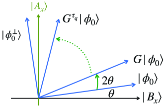
Figure 1: Illustration of the evolution in the two-dimensional plane.

When measuring $|\phi_{\tau_{q}}\rangle$, an outcome $i$ with $x_{i}=1$ occurs with probability

$$\varepsilon_{x}=\sin^{2}((2\tau_{q}+1)\theta)\geq\left(\frac{2\tau_{q}+1}{2}\theta\right)^{2}\geq\tau_{q}^{2}\sin^{2}\theta=\tau_{q}^{2}\frac{\alpha_{x}}{\omega}\,.$$

Thus

$$\varepsilon=\mathbb{E}_{x\leftarrow{D}}\varepsilon_{x}\geq\tau_{q}^{2}\frac{\mathbb{E}_{x}\alpha_{x}}{\omega}=\tau_{q}^{2}\frac{\sum_{i}\omega_{i}\sum_{x}d_{x}x_{i}}{\omega}=\tau_{q}^{2}\frac{\sum_{i}\omega_{i}^{2}}{\omega}\,.$$

∎

Optimality for permutation-invariant distributions.

Consider a special family of distributions, where $\omega_{i}$ are identical for all $i\in[m]$ implying that every $i$ is mapped to $1$ with equal probability. We call such a distribution ${D}$ permutation invariant, and in this case our quantum algorithm $\mathcal{A}$ becomes identical to the standard Grover’s algorithm. It also follows immediately Eq. 10 that for any $i,\omega_{i}=\nu_{D}$. Therefore we obtain that

$$\frac{\sum_{i}\omega_{i}^{2}}{\omega}=\frac{\sum_{i}\omega_{i}^{2}}{\sum_{i}\omega_{i}}=\frac{m\nu_{D}^{2}}{m\nu_{D}}=\nu_{D}\,.$$

As a result, the quantum algorithm $\mathcal{A}$ succeeds with probability $\Omega(\tau_{q}^{2}\nu_{D})$ in the case of permutation-invariant distribution, which is in turn optimal by our hardness bound (Theorem 2.1). This also reproves the tight quantum query complexity for multi-uniform search and Bernoulli search. We summarize it below.

Corollary 2.

For a permutation-invariant distribution ${D}$, the quantum algorithm $\mathcal{A}$ coincides with the standard Grover’s algorithm, and it succeeds with probability $\Omega(\tau_{q}^{2}\cdot\nu_{D})$ with $\tau_{q}$ quantum queries which is tight.

In particular, multi-uniform search and Bernoulli search have tight quantum query complexity $\Theta(\tau_{q}^{2}\frac{w}{m})$ and $\Theta(\tau_{q}^{2}\eta)$ for quantum algorithms with $\tau_{q}$ queries.

5 A Hybrid Algorithm for Distributional Search

We are now ready to describe a hybrid algorithm equipped with $\tau_{c}$ classical queries and $\tau_{q}$ quantum queries. The idea is simple: Given the distribution ${D}$, let $S=\{i_{1},...,i_{\tau_{c}}\}\subseteq[m]$ be the set of indices with the $\tau_{c}$ largest values of $\omega_{i}$. In case of ties, we break them arbitrarily. Our algorithm will first issue the $\tau_{c}$ classical queries on $S$ to verify if there exists any $i\in S$ such that $x_{i}=1$. If not, we run the quantum search algorithm $\mathcal{A}$ from before, but on the reduced search space $[m]-S$.

To run the quantum algorithm in a modular fashion, we can define an induced distribution $\tilde{D}$ on $\{0,1\}^{m-\tau_{c}}$. We will denote here by $x_{T}$ the substring of $x$ of size $|T|$ obtained from concatenating the bits $x_{i}$ for all $i\in T$ and we denote by $\bar{S}$ the set defined as $\bar{S}=[m]\backslash S$.

To define ${\tilde{}{D}}$, we first define $d:=\sum_{x\in\{0,1\}^{m}:x_{S}=0}d_{x}$. Then for each $\textbf{x}\in\{0,1\}^{m-\tau_{c}}$, we will define ${\tilde{d}}_{\textbf{x}}:=\frac{d_{x}}{d}$, where $x$ is the unique string with $x_{S}=0$ and $x_{\bar{S}}=\textbf{x}$. Note that there is a fixed mapping that matches every index $\textbf{i}\in\bar{S}$ with an index $i\in[m]$ such that $\textbf{x}_{\textbf{i}}=1$ if and only if $x_{i}=1$. We assume this mapping is performed implicitly whenever necessary. Therefore for every $\textbf{i}\in\bar{S}$, we can write the weight under ${\tilde{}{D}}$,

$${\tilde{\omega}}_{\textbf{i}}=\sum_{\textbf{x}\in\{0,1\}^{m-\tau_{c}}}{\tilde{d}}_{\textbf{x}}\cdot{\textbf{x}}_{\textbf{i}}=\frac{\sum_{x:x_{S}=0}d_{x}\cdot x_{i}}{\sum_{x:x_{S}=0}d_{x}}\,.$$

Our hybrid algorithm can now be described as follows. Hybrid Search Algorithm $\mathcal{A}_{h}$ for an arbitrary distribution ${D}$ Given: $x\in\{0,1\}^{m}$ drawn from ${D}$ as a black-box function. Goal: find $i\in[m]$ such that $x_{i}=1$ making $\tau_{c}$ classical queries $\tau_{q}$ and quantum queries to $x$. Classical Stage. $\mathcal{A}$ makes classical queries for each $i\in S$, where $S$ as defined above consists of the indices with the $\tau_{c}$ largest $\omega_{i}$. If some $x_{i}=1$, output $i$ and abort. Otherwise, continue. Quantum Stage. Run the quantum algorithm $\mathcal{A}$ on the induced distribution ${\tilde{}{D}}$.

The success probability can be split into analyzing the classical and quantum stages separately as we show below. First, we define the following binary random variables:

• $Z_{c}^{x}=1$ if and only if $x_{i}=1$ for some $i\in S$ (the classical stage succeeds);

• $Z_{q}^{x}=1$ if and only if the quantum stage is successful.

Lemma 13.

For any distribution ${D}$, the probability that hybrid algorithm $\mathcal{A}_{h}$ succeeds is

$$\Pr[\mathsf{Hybrid\ Success}]\geq\frac{1}{2}\left(\mathbb{E}_{x\leftarrow{D}}[Z_{c}^{x}]+\mathbb{E}_{x\leftarrow{D}}[Z_{q}^{x}]\right)\,.$$

Proof.

The algorithm fails if both classical and quantum stages fail. Hence the failure probability is

$$\mathbb{E}_{x\leftarrow{D}}[(1-Z_{c}^{x})(1-Z_{q}^{x})]=1-\mathbb{E}_{x\leftarrow{D}}[Z_{c}^{x}]-\mathbb{E}_{x\leftarrow{D}}[Z_{q}^{x}]+\mathbb{E}_{x\leftarrow{D}}[Z_{c}^{x}\cdot Z_{q}^{x}]\,.$$

Then by using the Cauchy-Schwartz inequality (Lemma 2) and as $Z_{c}^{x}$ and $Z_{q}^{x}$ are both binary variables, we have

$$\mathbb{E}_{x\leftarrow{D}}[Z_{c}^{x}\cdot Z_{q}^{x}] \leq\sqrt{\mathbb{E}_{x\leftarrow{D}}[Z_{c}^{x}]\cdot\mathbb{E}_{x\leftarrow{D}}[Z_{q}^{x}]}$$

$$\leq\frac{1}{2}(\mathbb{E}_{x\leftarrow{D}}[Z_{c}^{x}]+\mathbb{E}_{x\leftarrow{D}}[Z_{q}^{x}])\,.$$

We can then conclude that the algorithm’s success probability is

$$\Pr[\mathsf{Hybrid\ Success}]=1-\mathbb{E}_{x\leftarrow{D}}[(1-Z_{c}^{x})(1-Z_{q}^{x})]\geq\frac{1}{2}\left(\mathbb{E}_{x\leftarrow{D}}[Z_{c}^{x}]+\mathbb{E}_{x\leftarrow{D}}[Z_{q}^{x}]\right)\,.$$

∎

By Theorem 4.1, we can immediately give an expression for the quantum success probability. Namely,

$$\mathbb{E}_{x\leftarrow{D}}[Z_{q}^{x}]\geq\tau_{q}^{2}\frac{\sum_{\textbf{i}\in\bar{S}}{\tilde{\omega}}_{\textbf{i}}^{2}}{\sum_{\textbf{i}\in\bar{S}}{\tilde{\omega}}_{\textbf{i}}}\,.$$

5.1 Success Probability for Special Distributions

We now show that for some special cases the hybrid algorithm above is optimal. We note that in these cases, the quantum stage actually coincides with the standard Grover search, and the quantum success probability can be obtained by the known result. Our analysis can be viewed as an alternative approach following the general result of Theorem 4.1.

When $x\leftarrow{D}$ assigns a single $i$ with $x_{i}=1$ uniformly at random, ${\tilde{}{D}}$ can be seen as the same distribution but restricting to $x$ with $x_{S}=0$. For all $\textbf{i}\in\bar{S}$, we have ${\tilde{\omega}}_{\textbf{i}}=\frac{1}{m-c}$, and hence:

$$\mathbb{E}_{x\leftarrow{D}}[Z_{q}^{x}]=\tau_{q}^{2}\cdot\frac{\sum_{\textbf{i}\in\bar{S}}{\tilde{\omega}}_{\textbf{i}}^{2}}{\sum_{\textbf{i}\in\bar{S}}{\tilde{\omega}}_{\textbf{i}}}=\tau_{q}^{2}\frac{1}{m-c}\,.$$

It is also easy to observe that $\mathbb{E}_{x\leftarrow{D}}[Z_{c}^{x}]=\tau_{c}\frac{1}{m}$.

Lemma 14 (Uniform Hybrid Query Complexity).

When ${D}$ is the uniform distribution, our hybrid algorithm equipped with $\tau_{c}$ classical queries and $\tau_{q}$ quantum queries succeeds with probability

$$\Pr[\mathsf{Hybrid\ Success}]\geq\frac{1}{2}\left(\frac{\tau_{c}}{m}+\frac{\tau_{q}^{2}}{m-\tau_{c}}\right).$$

Modulo constant factors and lower order terms, this matches the hardness bound, and hence the hybrid query complexity is $\Theta\left(\frac{1}{m}(\tau_{c}+\tau_{q}^{2})\right)$.

Similarly, we can obtain a tight bound for the Bernoulli distribution, by the observation that ${\tilde{}{D}}$ in this case is just another Bernoulli with the same $\eta$. Hence

$$\mathbb{E}_{x\leftarrow{D}}[Z_{q}^{x}]=\eta\cdot\tau_{q}^{2}\,.$$

On the other hand,

$$\mathbb{E}_{x\leftarrow{D}}[Z_{c}^{x}]=1-(1-\eta)^{\tau_{c}}\geq\frac{1}{2}\eta\cdot\tau_{c}\,.$$

Lemma 15 (Bernoulli Hybrid Success and Optimality).

When ${D}$ is the Bernoulli distribution, our hybrid algorithm equipped with $\tau_{c}$ classical queries and $\tau_{q}$ quantum queries succeeds with probability at least:

$$\Pr[\mathsf{Hybrid\ Success}]\geq\frac{1}{2}\eta\left(\frac{1}{2}\tau_{c}+\tau_{q}^{2}\right)\,.$$

Hence the hybrid query complexity for the Bernoulli distribution is $\Theta(\eta(\tau_{c}+\tau_{q}^{2}))$.

References

• ABKM [22] Gorjan Alagic, Chen Bai, Jonathan Katz, and Christian Majenz. Post-quantum security of the even-mansour cipher. In Advances in Cryptology – EUROCRYPT 2022, pages 458–487. Springer, 2022.
• AHU [19] Andris Ambainis, Mike Hamburg, and Dominique Unruh. Quantum security proofs using semi-classical oracles. In Advances in Cryptology – CRYPTO 2019, pages 269–295. Springer, 2019.
• AMRS [20] Gorjan Alagic, Christian Majenz, Alexander Russell, and Fang Song. Quantum-secure message authentication via blind-unforgeability. In Advances in Cryptology – EUROCRYPT 2020. Springer, 2020.
• ARU [14] Andris Ambainis, Ansis Rosmanis, and Dominique Unruh. Quantum attacks on classical proof systems: The hardness of quantum rewinding. In 2014 IEEE 55th Annual Symposium on Foundations of Computer Science, pages 474–483. IEEE, 2014.
• BBBV [97] Charles H Bennett, Ethan Bernstein, Gilles Brassard, and Umesh Vazirani. Strengths and weaknesses of quantum computing. SIAM journal on Computing, 26(5):1510–1523, 1997.
• BDF+ [11] Dan Boneh, Özgür Dagdelen, Marc Fischlin, Anja Lehmann, Christian Schaffner, and Mark Zhandry. Random oracles in a quantum world. In Advances in Cryptology – ASIACRYPT 2011, pages 41–69. Springer, 2011.
• BR [93] Mihir Bellare and Phillip Rogaway. Random oracles are practical: A paradigm for designing efficient protocols. In Proceedings of the 1st ACM conference on Computer and Communications Security, pages 62–73, 1993.
• BR [94] Mihir Bellare and Phillip Rogaway. Optimal asymmetric encryption. In Advances in Cryptology–EUROCRYPT 1994, pages 92–111. Springer, 1994.
• BR [96] Mihir Bellare and Phillip Rogaway. The exact security of digital signatures-how to sign with rsa and rabin. In Advances in Cryptology–Eurocrypt 1996, pages 399–416. Springer, 1996.
• BZ [13] Dan Boneh and Mark Zhandry. Secure signatures and chosen ciphertext security in a quantum computing world. In Advances in Cryptology – CRYPTO 2013, pages 361–379. Springer, 2013.
• CCHL [22] Sitan Chen, Jordan Cotler, Hsin-Yuan Huang, and Jerry Li. The complexity of nisq, 2022.
• CCL [23] Nai-Hui Chia, Kai-Min Chung, and Ching-Yi Lai. On the need for large quantum depth. J. ACM, 70(1), jan 2023.
• CEV [23] Céline Chevalier, Ehsan Ebrahimi, and Quoc-Huy Vu. On security notions for encryption in a quantum world. In Progress in Cryptology – INDOCRYPT 2022, pages 592–613. Springer, 2023.
• CGK+ [23] Alexandru Cojocaru, Juan Garay, Aggelos Kiayias, Fang Song, and Petros Wallden. Quantum Multi-Solution Bernoulli Search with Applications to Bitcoin’s Post-Quantum Security. Quantum, 7:944, 2023.
• CM [20] Matthew Coudron and Sanketh Menda. Computations with greater quantum depth are strictly more powerful (relative to an oracle). In Proceedings of the 52nd Annual ACM SIGACT Symposium on Theory of Computing, STOC 2020, page 889–901, New York, NY, USA, 2020. Association for Computing Machinery.
• CMS [19] Alessandro Chiesa, Peter Manohar, and Nicholas Spooner. Succinct arguments in the quantum random oracle model. In 17th International Theory of Cryptography Conference – TCC 2019, pages 1–29. Springer, 2019.
• DFMS [19] Jelle Don, Serge Fehr, Christian Majenz, and Christian Schaffner. Security of the Fiat-Shamir transformation in the quantum random-oracle model. In Advances in Cryptology – CRYPTO 2019, pages 356–383. Springer, 2019.
• DFMS [22] Jelle Don, Serge Fehr, Christian Majenz, and Christian Schaffner. Online-extractability in the quantum random-oracle model. In Advances in Cryptology – EUROCRYPT 2022, pages 677–706. Springer, 2022.
• DH [09] Cătălin Dohotaru and Peter Høyer. Exact quantum lower bound for grover’s problem. Quantum Information & Computation, 9(5):533–540, 2009.
• ES [15] Edward Eaton and Fang Song. Making Existential-unforgeable Signatures Strongly Unforgeable in the Quantum Random-oracle Model. In 10th Conference on the Theory of Quantum Computation, Communication and Cryptography – TQC 2015, volume 44 of Leibniz International Proceedings in Informatics (LIPIcs), pages 147–162. Schloss Dagstuhl–Leibniz-Zentrum fuer Informatik, 2015.
• ES [20] Edward Eaton and Fang Song. A note on the instantiability of the quantum random oracle. In International Conference on Post-Quantum Cryptography, pages 503–523. Springer, 2020.
• FO [13] Eiichiro Fujisaki and Tatsuaki Okamoto. Secure integration of asymmetric and symmetric encryption schemes. Journal of Cryptology, 26(1):80–101, 2013. Preliminary version in CRYPTO 1999.
• FOPS [04] Eiichiro Fujisaki, Tatsuaki Okamoto, David Pointcheval, and Jacques Stern. RSA-OAEP is secure under the rsa assumption. Journal of Cryptology, 17(2):81–104, 2004. Preliminary version in CRYPTO 2001.
• GKL [15] Juan Garay, Aggelos Kiayias, and Nikos Leonardos. The bitcoin backbone protocol: Analysis and applications. In Advances in Cryptology – EUROCRYPT 2015, pages 281–310. Springer, 2015.
• Gro [96] Lov K Grover. A fast quantum mechanical algorithm for database search. In Proceedings of the twenty-eighth annual ACM symposium on Theory of computing, pages 212–219. ACM, 1996.
• HHK [17] Dennis Hofheinz, Kathrin Hövelmanns, and Eike Kiltz. A modular analysis of the fujisaki-okamoto transformation. In 15th International Theory of Cryptography Conference – TCC 2017, pages 341–371. Springer, 2017.
• HLS [22] Yassine Hamoudi, Qipeng Liu, and Makrand Sinha. Quantum-classical tradeoffs in the random oracle model, 2022.
• HRS [16] Andreas Hülsing, Joost Rijneveld, and Fang Song. Mitigating multi-target attacks in hash-based signatures. In 19th IACR International Conference on Public-Key Cryptography — PKC 2016, pages 387–416. Springer, 2016.
• JST [21] Joseph Jaeger, Fang Song, and Stefano Tessaro. Quantum key-length extension. In 19th International Theory of Cryptography Conference – TCC 2021, pages 209–239. Springer, 2021.
• KM [10] Hidenori Kuwakado and Masakatu Morii. Quantum distinguisher between the 3-round feistel cipher and the random permutation. In 2010 IEEE International Symposium on Information Theory, pages 2682–2685. IEEE, 2010.
• Pre [18] John Preskill. Quantum computing in the NISQ era and beyond. Quantum, 2:79, 2018.
• Ros [22] Ansis Rosmanis. Hybrid quantum-classical search algorithms. arXiv preprint arXiv:2202.11443, 2022.
• Sho [01] Victor Shoup. OAEP reconsidered. In Advances in Cryptology—-CRYPTO 2001, pages 239–259. Springer, 2001.
• SZ [19] Xiaoming Sun and Yufan Zheng. Hybrid decision trees: Longer quantum time is strictly more powerful, 2019.
• Unr [15] Dominique Unruh. Non-interactive zero-knowledge proofs in the quantum random oracle model. In Advances in Cryptology – EUROCRYPT 2015, pages 755–784. Springer, 2015.
• YZ [21] Takashi Yamakawa and Mark Zhandry. Classical vs quantum random oracles. In Advances in Cryptology – EUROCRYPT 2021, pages 568–597. Springer, 2021.
• Zal [99] Christof Zalka. Grover’s quantum searching algorithm is optimal. Physical Review A, 60(4):2746, 1999.
• Zha [15] Mark Zhandry. Secure identity-based encryption in the quantum random oracle model. International Journal of Quantum Information, 13(04):1550014, 2015. Preliminary version in IACR CRYPTO 2012.
• Zha [19] Mark Zhandry. How to record quantum queries, and applications to quantum indifferentiability. In Advances in Cryptology – CRYPTO 2019, pages 239–268. Springer, 2019.
• Zha [21] Mark Zhandry. How to construct quantum random functions. Journal of the ACM (JACM), 68(5):1–43, 2021. Preliminary version in FOCS 2012.