Abstract

We optimize pipeline parallelism for deep neural network (DNN) inference by partitioning model graphs into $k$ stages and minimizing the running time of the bottleneck stage, including communication. We design practical algorithms for this NP-hard problem and show that they are nearly optimal in practice by comparing against strong lower bounds obtained via novel mixed-integer programming (MIP) formulations. We apply these algorithms and lower-bound methods to production models to achieve substantially improved approximation guarantees compared to standard combinatorial lower bounds. For example, evaluated via geometric means across production data with $k=16$ pipeline stages, our MIP formulations more than double the lower bounds, improving the approximation ratio from $2.175$ to $1.058$. This work shows that while max-throughput partitioning is theoretically hard, we have a handle on the algorithmic side of the problem in practice and much of the remaining challenge is in developing more accurate cost models to feed into the partitioning algorithms.

1 Introduction

Large-scale machine learning (ML) workloads rely on distributed systems and specialized hardware, e.g., graphics processing units (GPUs) and tensor processing units (TPUs). Fully utilizing this hardware, however, remains a challenging and increasingly important problem. ML accelerators have both a small amount of fast memory co-located with each computational unit (CU), and a much larger amount of slow memory that is accessed via an interconnect shared among the CUs. Achieving peak performance for deep neural network (DNN) training and inference requires the ML compiler and/or practitioner to pay significant attention to where intermediate data is stored and how it flows between CUs. This work focuses on pipeline partitioning for DNNs to maximize inference throughput and lower bound methods for provable performance guarantees.

ML inference handles two main types of data: model parameters (weights learned during training) and activations (intermediate outputs of the model, e.g., from a hidden layer). Keeping activations in fast memory (e.g., SRAM) is critical, and often treated by ML compilers as a hard constraint. Model parameters can be streamed from slow memory, but caching them in fast memory greatly boosts performance. When we partition an end-to-end inference computation into a linear pipeline with $k$ stages and process each stage on a different CU, we increase the amount of fast memory at our disposal by a factor of $k$, allowing us to cache more parameters and support larger activations (and hence use larger models and/or batch sizes). However, this introduces two main challenges: (1) CUs must send their outputs downstream, often via a slow and contended data channel, so we need to partition the computation graph to minimize communication overhead; and (2) we must balance the running time across all stages of the partition since the overall throughput is governed by the bottleneck stage.

1.1 Our contributions and techniques

We summarize the main contributions of this work:

1. We formalize the max-throughput partitioning problem (MTPP) for pipelined inference, show it is NP-hard, and present a fast and effective algorithm that combines topological sorting, dynamic programming, and a biased random-key genetic algorithm.

2. We formulate a novel mixed-integer program (MIP) for MTPP and sparse relaxations of it to obtain strong lower bounds (Section 4).

3. We present extensive experiments across real and synthetic computation graphs for a wide variety of model architectures and ML workloads (DNNs and more). Using our MIP lower bounds, we prove (a posteriori) that our partitioning algorithms are highly effective in practice, e.g., within 5.8% of optimal for $k\leq 16$ stages on a production benchmark, whereas standard lower bounds provide only a 2.175-approximation.

2 Preliminaries

To build intuition, it is helpful to think of pipelined inference as an assembly line where the model is split into $k$ stages and the inputs for each stage are produced earlier in the assembly line. If $t$ is the running time of the longest (i.e., bottleneck) stage, then each stage can finish its local computation in parallel in time $t$. Every $t$ units of time we can advance each batch one stage forward in the assembly line (Figure 1), so the end-to-end latency for a batch of inferences is $kt$ and the throughput of the system is $\nicefrac{{1}}{{t}}$ (i.e., 1 batch per $t$ units of time). It is therefore critical to partition work to minimize the bottleneck time $t$.

Pipeline parallelism has been used heavily in ML systems to scale up DNN training, e.g., GPipe (Huang et al., 2019) and PipeDream (Narayanan et al., 2019; 2021). See Section 6 for more details. In contrast, our work focuses strictly on partitioning large models to have high inference throughput, so that they can easily be deployed across ML accelerators and used in high-QPS systems.

2.1 Computation graphs

A machine learning model is commonly represented as a computation graph $G=(V,E)$, where $V$ is the set of node operations (called ops) and $E\subseteq V\times V$ is the set of data flow edges. Let $n=|V|$ and $m=|E|$. For simplicity, assume each op $u$ outputs one tensor that is consumed by (possibly many) downstream ops $v$, represented by edges $(u,v)$. This corresponds to a tensorflow.Graph (Abadi et al., 2016), and has MLIR (Lattner et al., 2021), MXNet (Chen et al., 2015), and PyTorch (Paszke et al., 2019) analogs.

We introduce several node weights to help model the cost of pipelined inference:

• $\textnormal{{work}}(v)$ is the running time of $v\in V$. This is typically estimated with an analytic or learned cost model (Kaufman et al., 2021).

• $\texttt{size}_{\texttt{param}}(v)$ is the memory footprint of the model parameters that $v\in V$ uses. For example, if $v$ is a matrix multiplication op, $\texttt{size}_{\texttt{param}}(v)$ is the storage cost for the entries of the matrix.

• $\texttt{size}_{\texttt{out}}(v)$ is the size of the output of $v$ (e.g., in bytes).

We use standard graph theory notation to denote the dependencies between nodes:

• $N^{-}(v)=\{u\in V:(u,v)\in E\}$ is the set of nodes whose output is consumed by $v$.

• $N^{+}(v)=\{w\in V:(v,w)\in E\}$ is the set of nodes that consume the output of $v$.

• $N^{-}(S)=\bigcup_{v\in S}N^{-}(v)\setminus S$ and $N^{+}(S)=\bigcup_{v\in S}N^{+}(v)\setminus S$ extend neighborhood notation to sets of nodes.

The reason for subtracting $S$ from the neighborhoods will become clear when we consider inter-block communication costs for a partition of $G$.

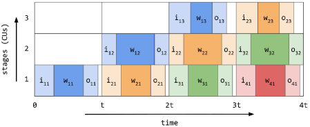
Figure 1: Example pipeline from startup to steady state with $k=3$ stages. Each inference batch is represented with the same color as it advances through the pipeline. The values $\texttt{i}_{b\ell}$, $\texttt{w}_{b\ell}$, $\texttt{o}_{b\ell}$ are the times needed for stage $\ell$ to get its input for batch $b$, process it, and flush its output. Stage $2$ is the bottleneck, i.e., $t=\texttt{i}_{*2}+\texttt{w}_{*2}+\texttt{o}_{*2}$, and limits the system throughput. Empty space (white) denotes that a computational unit is idle.

2.2 Problem statement

Acyclic quotient graph constraint

Let $\mathcal{P}_{k}(G)$ be the set of partitions of $V$ into $k$ blocks (possibly empty) such that the induced quotient graph of $G$ is acyclic. Formally, let $P=\{P_{1},P_{2},\dots,P_{k}\}$ be a partition of $V$, i.e., $P_{1}\cup P_{2}\cup\dots\cup P_{k}=V$ and $P_{i}\cap P_{j}=\varnothing$ for all $i\neq j$. Since $P_{i}$ can be empty, we can alternatively think about partitioning $V$ into at most $k$ blocks. For each $v\in V$, let $[v]_{P}$ denote the block in $P$ containing $v$. The quotient graph $Q=(P,E^{\prime})$ for partition $P$ has the blocks of $P$ as its nodes and reduced edge set $E^{\prime}=\{([u]_{P},[v]_{P}):(u,v)\in E\text{~{}and~{}}[u]_{P}\neq[v]_{P}\}$. We require $Q$ to be acyclic so that we have valid data flow when $G$ is partitioned across different processors.

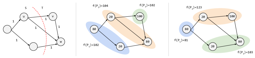
Figure 2: Computation graph partitioning examples: (left) tensor cut property where $\textnormal{{io}}(S,T)=2$ since $v$ and $w$ consume the same data; (middle) invalid partition because blocks $P_{2}$ and $P_{3}$ form a cycle in the quotient graph; (right) valid partition with block costs for $k=3$.

Inter-block communication

Let $B$ be the bandwidth of the interconnect between blocks. For disjoint sets $S,T\subseteq V$, the IO cost (in units of time) from $S$ to $T$ is

$$\textnormal{{io}}(S,T)=\frac{1}{B}\sum_{v\in N^{-}(T)\cap S}\texttt{size}_{\texttt{out}}(v).$$ (1)

We overload singleton notation: $\textnormal{{io}}(u,v)=\textnormal{{io}}(\{u\},\{v\})$.

By summing over the set of producer ops $v\in N^{-}(T)\cap S$, each tensor going from $S$ to $T$ is counted once, even if it has many consumers in $T$. This is different from the cost of the traditional edge-cut set since it considers only one edge in each tensor edge equivalence class (see Figure 2). Refining how communication costs are modeled is where computation graph partitioning starts to deviate from more familiar cut-based graph partitioning problems.

Streaming model parameters

Each block is a computational unit with a fixed amount of fast memory, e.g., SRAM for GPUs and multi-chip packages (Mei & Chu, 2016, Gao et al., 2020, Dasari et al., 2021) or high-bandwidth memory for TPUs (Jouppi et al., 2017; 2023). To achieve peak performance, it is critical that all model parameters assigned to a block are fully cached in fast memory. Otherwise, some of the model parameters must be streamed to the block during each batch of inference from slow memory, e.g., shared DRAM. Inter-block bandwidth is often at least an order of magnitude slower than intra-block bandwidth (Dao et al., 2022), so we ignore communication between ops within a block and refer to the time needed to stream parameters that spill over as the overflow cost of a block.

There are two key factors for deciding if model parameters can be fully cached on a block: (1) the available amount of fast memory, and (2) the peak activation memory. We start by describing the peak memory scheduling problem (Marchal et al., 2019, Paliwal et al., 2020, Ahn et al., 2020, Lin et al., 2021, Vee et al., 2021, Zhang et al., 2022). For a set of ops $P_{i}$, peak memory scheduling asks to find a linear execution order of $v\in P_{i}$ that minimizes the amount of working memory needed for all intermediate computations. Once we know how much fast memory to reserve for activations, we allocate the rest for caching model parameters.

The overflow cost for a set of ops $S\subseteq V$ on a block with $M$ fast memory, peak memory $\texttt{peak}(S)$, and inter-block bandwidth $B$ is

$$\textnormal{{overflow}}(S)=\frac{\left(\texttt{size}_{\texttt{param}}(S)+\texttt{peak}(S)-M\right)^{+}}{B},$$ (2)

where we use the notation $x^{+}=\max(x,0)$.

Overall block cost

The cost of a block with nodes $S\subseteq V$ (i.e., its running time) in a pipeline partition is

$$f(S) =\overbrace{\textnormal{{io}}(V\setminus S,S)}^{\text{input tensors}}+\sum_{v\in S}\textnormal{{work}}(v)+\textnormal{{overflow}}(S)$$

$$+\overbrace{\textnormal{{io}}(S,V\setminus S)}^{\text{output tensors}}.$$ (3)

Eq. Section 2.2 models the higher-order terms in the running time of block $S$. In particular, it ignores intra-block communication between nodes in $S$ since activations are stored in fast memory. The dominant costs are: (1) getting tensor inputs from upstream blocks, (2) processing these inputs and streaming op parameters if not cached, and (3) outputting tensors for downstream stages. Putting everything together, we arrive at the following min-max objective function.

Definition 2.1.

For a computation graph $G$ and number of blocks $k$, the max-throughput partitioning problem (MTPP) is

$$P^{*}=\operatorname*{arg\,min\,}_{P\in\mathcal{P}_{k}(G)}\left\{\max_{i\in[k]}f(P_{i})\right\},$$ (4)

where $[k]=\{1,\dots,k\}$. Let $\textnormal{OPT}=\max_{i\in[k]}f(P^{*}_{i})$ denote the minimum bottleneck cost.

Remark 2.2.

There are many more moving parts to ML performance than graph partitioning—it is just one of many ML compiler passes (e.g., op fusion, tensor sharding, fine-grained subgraph partitioning, peak memory scheduling). However, it is one of the highest-order components with a significant impact on overall system efficiency.

3 Algorithms

Now we present computation graph partitioning algorithms for high-throughput pipelined inference. We start by giving a reduction from the minimum makespan scheduling problem  (Hochbaum & Shmoys, 1987) to show that MTPP is NP-hard and cannot have a fully polynomial-time approximation scheme (FPTAS), unless $\textnormal{P}=\textnormal{NP}$. Then we design a fast and effective heuristic using Kahn’s algorithm, segment trees, and dynamic programming. This approach can also be extended with genetic algorithms. Our algorithms are simple by design so that they can run inside ML compilers with tight latency requirements (e.g., XLA for TensorFlow). In Section 4 and Section 5, we prove that these algorithms are near-optimal in practice by computing novel per-instance approximation guarantees (i.e., certificates) via new mixed-integer programming formulations.

3.1 Hardness

We reduce from minimum makespan scheduling on $k$ identical parallel processors, which is strongly NP-hard.

Theorem 3.1.

For $k=2$, MTPP is NP-hard. Furthermore, there does not exist a fully polynomial-time approximation scheme for MTPP, unless $\textnormal{P}=\textnormal{NP}$.

Proof.

The minimum makespan scheduling problem on $k$ identical parallel processors is as follows. We are given processing times for $n$ jobs $(p_{1},p_{2},\dots,p_{n})$ and asked to find an assignment of jobs to processors so that the completion time (i.e., makespan) is minimized. We reduce to MTPP by constructing a graph $G$ with $n$ vertices and no edges, setting $\textnormal{{work}}(v_{i})=p_{i}$, and computing a max-throughput partition of $G$ to solve the original makespan instance.

For $k=2$, this is the NP-hard partition problem. More generally, minimum makespan scheduling is strongly NP-hard, so there cannot exist an FPTAS, unless $\textnormal{P}=\textnormal{NP}$ (Hochbaum & Shmoys, 1987). ∎

3.2 Reducing to a search over topological orderings

Next, we reduce MTPP to a search over topological orderings as follows:

1. An optimal partition $P^{*}$ in Eq. Equation 4 has a corresponding topological order $\pi^{*}$.

2. There exist node weights $\mathbf{x}^{*}\in[0,1]^{n}$ such that Kahn’s algorithm with tiebreaking (Algorithm 3) on $\mathbf{x}^{*}$ recovers $\pi^{*}$.

3. For any topological order $\pi\in\mathfrak{S}_{V}$, we can efficiently find an optimal “stars-and-bars” partition of $\pi$ with dynamic programming. By slicing a topological order this way, we easily satisfy the acyclicity constraint.

One method for generating different topological orders is to sample random node weights for Item 2. Another approach is to learn good weights using, e.g., genetic algorithms or reinforcement learning. To implement the dynamic program in Item 3 efficiently, we use a data structure for “segment-cost” queries and pseudocode for the SliceGraph algorithm. All of the missing proofs in this section are deferred to Appendix A.

Lemma 3.2.

There is a SegmentCostDataStructure that takes computation graph $G=(V,E)$ and topological order $\pi\in\mathfrak{S}_{V}$ as input, and supports the following operations:

• $\textnormal{{Initialize}}(G,\pi)$: Preprocesses the graph in $O(n^{2}+m\log^{2}(n))$ time.

• $\textnormal{{Query}}(\ell,r)$: Returns $f(\{v_{\pi(\ell)},\dots,v_{\pi(r)}\})$ in Eq. Section 2.2 in constant time, after initialization.

At a high level, SegmentCostDataStructure computes the cost of each $[\ell,r]$ slice of topological order $\pi$ (counting each tensor in a cut once) using a sliding window algorithm and two-dimensional Fenwick tree (Mishra, 2013).

Algorithm 1 Optimal MTPP slicing of topological order $\pi$ into at most $k$ blocks.

1:function SliceGraph($G$, $k$, $\pi$)

2:// Partitions the full topological order $\pi$

3:     Initialize segment_cost data structure for $(G,\pi$)

4:     return $\textnormal{{DP}}(\texttt{segment\_cost},n,k)$

5:function DP(segment_cost, $r$, $k^{\prime}$)

6:// Recursively partitions the first $r$ nodes optimally into $k^{\prime}$ blocks

7:     if $k^{\prime}=1$ then

8:         return $\texttt{segment\_cost}.\texttt{Query}(1,r)$      

9:     $ans\leftarrow\infty$

10:     for $\ell=1$ to $r$ do

11:         $a\leftarrow\textnormal{{DP}}(\texttt{segment\_cost},\ell,k^{\prime}-1)$

12:         $b\leftarrow\texttt{segment\_cost}.\texttt{Query}(\ell+1,r)$

13:         $ans\leftarrow\min(ans,\max(a,b))$      

14:     return $ans$

Lemma 3.3.

SliceGraph runs in time $O(n^{2}k+m\log^{2}(n))$ and finds an optimal stars-and-bars partition for topological order $\pi$ of $G$ into at most $k$ blocks for MTPP.

The correctness of Lemma 3.3 immediately follows from applying dynamic programming to Eq. Equation 4. While the running time might initially seem slow, computation graphs are often small in practice (e.g., $n\leq 1000$ and $m\leq 2000$), even though they can have a massive number of model parameters. It is an interesting algorithmic problem to improve the running time; however, we note that the $\max(a,b)$ in 13 of the recurrence of Algorithm 1 is non-convex in $\ell$, so we cannot use dynamic programming techniques like the “convex hull trick” to reduce the $O(n^{2}k)$ term to $O(nk\log n)$ after initializing the SegmentCostDataStructure.

3.3 Searching over topological orders

Any topological order $\pi\in\mathfrak{S}_{V}$ can be realized using Kahn’s algorithm with the right node priorities $\mathbf{x}\in[0,1]^{n}$ for tie breaking, so we focus on methods for learning good vectors of node weights. Note that we have only recast MTPP into a search over topological orders to ease the acyclic quotient graph constraint so far—it is still provably hard to find an optimal topological order. The following results formalize these observations.

Theorem 3.4.

There exist node priorities $\mathbf{x}^{*}\in[0,1]^{n}$ such that Kahn’s algorithm with tie-breaking outputs a topological order $\pi^{*}$ for which $\textnormal{{SliceGraph}}(G,k,\pi^{*})=\textnormal{OPT}$.

Proof.

Let $P^{*}$ be an optimal MTPP partition of the nodes, and let $Q=(P^{*},E^{\prime})$ be the induced acyclic quotient graph on the blocks. Let $\sigma$ be a topological ordering of the blocks $P^{*}$ in $Q$. Then, set $x^{*}_{v}\leftarrow k-\sigma^{-1}[[v]_{P^{*}}]$ for every $v\in V$, where $[v]_{P}$ denotes the block index $i\in[k]$ of the partition $P=\{P_{1},P_{2},\dots,P_{k}\}$ and $\sigma^{-1}$ is the inverse permutation of $\sigma\in\mathfrak{S}_{P^{*}}$. This means nodes appearing in the first block of $P^{*}$ according to $\sigma$ have highest priority. Running Kahn’s algorithm with $\mathbf{x}^{*}$ recovers a topological order $\pi^{*}\in\mathfrak{S}_{V}$ such that when optimally segmented into $k$ blocks, has an objective value that is equal to partition $P^{*}$. ∎

Kahn’s algorithm

Kahn’s algorithm (Kahn, 1962) is a topological sorting algorithm that iteratively peels off the leaves of a DAG. It is particularly useful since it can output different orderings—if there are multiple leaves, different tie-breaking rules give different topological orders. We use KahnWithNodePriorities (Algorithm 3), which takes a vector $\mathbf{x}\in[0,1]^{n}$ of node priorities as input and runs in time $O(n\log n+m)$ when implemented with a heap-based priority queue for the active set of leaves.

Heuristics for node priorities

Since it is NP-hard to find an optimal topological order $\pi^{*}$, we present heuristics that are provably close to optimal on our real-world datasets.

Random weights. Each node weight $x_{i}\sim U(0,1)$ is drawn independently and uniformly at random. In Section 5, we show this is surprisingly effective in practice due to the typical structure of DNN computation graphs. This is not the same as sampling topological orders uniformly at random, which has its own rich history (Matthews, 1991, Karzanov & Khachiyan, 1991, Bubley & Dyer, 1999, Wilson, 2004, Huber, 2006, Bhakta et al., 2017, García-Segador & Miranda, 2019).

Biased random-key genetic algorithm (BRKGA). BRKGA is a problem-agnostic metaheuristic that evolves real-valued vectors $\mathbf{x}\in[0,1]^{N}$ called chromosomes using a decoder function that links BRKGA’s evolutionary rules to the problem at hand (Gonçalves & Resende, 2011). We use BRKGA to learn good node priorities by evaluating the quality of each induced partition $P(\mathbf{x})$. In the language of genetic algorithms, the fitness of $\mathbf{x}$ is the MTPP objective value $\max_{i\in[k]}f_{P(\mathbf{x})}(i)$. We present this decoder in Algorithm 2.

Algorithm 2 BRKGA decoder using Kahn’s algorithm and SliceGraph to partition $G$.

1:function BrkgaSortAndSliceDecoder($G$, $k$, chromosome $\mathbf{x}\in[0,1]^{n}$ of node priorities)

2:     $\pi\leftarrow\textnormal{{KahnWithNodePriorities}}(G,\mathbf{x})$

3:     return $\textnormal{{SliceGraph}}(G,k,\pi)$

In contrast, however, even with optimal topological order slicing, there exist worst-case instances $(k,G,\pi)$, for any $k\geq 2$, that can be as bad as the trivial MTPP algorithm that puts all nodes into the same block.

Lemma 3.5.

For any $k\geq 2$, there is a computation graph $G$ and topological order $\pi$ such that when optimally sliced, $\textnormal{{SliceGraph}}(G,k,\pi)=k\cdot\textnormal{OPT}$.

We give these graph construction in Appendix A.

4 Lower bounds via mixed-integer programming

Figure 3: Exact MIP for solving MTPP, where variables $x_{vb}\in\{0,1\}$ indicate whether node $v\in V$ is assigned to block $b\in[k]$.

In this section, we formulate a novel MIP to solve MTPP in Eq. Equation 4. Even for medium-sized models and moderate values of $k$, this program pushes the limits of MIP solvers. We then show how to relax the formulation to give strong lower bounds with fewer variables, constraints, and non-zeros. The exact MIP and the lower bound relaxations are the main theoretical contribution of this work, allowing us to prove offline per-instance approximation guarantees.

To simplify our presentation, we ignore the overflow terms in Eq. Section 2.2 since $\texttt{peak}(S)$ depends on how the ops in a block are scheduled (Paliwal et al., 2020). This is equivalent to setting aside an activation buffer for each block and treating the remaining amount of fast memory as the new budget.

4.1 Exact MIP formulation

Here we present a MIP for solving MTPP (Figure 3). The main idea is to number the blocks from $1$ to $k$ in DAG order (i.e., a topological order of the induced quotient graph) and use binary decision variables to assign nodes to blocks.

Decision variables

There are $O(nk)$ binary decision variables:

• $x_{vb}$ indicates whether node $v\in V$ is assigned to block $b\in[k]$.

• $y_{vb}$ indicates whether node $v\in V$ is assigned to some block at or before $b$. For any feasible assignment, this means $y_{vk}=1$, for all $v\in V$, and $y_{v(b-1)}\leq y_{vb}$, for all $v\in V,b\in[k]$, where we let $y_{v0}=0$ for notational convenience.

• $c_{ub}$ indicates whether any of the edges $(u,v)\in E$, corresponding to the tensor that $u$ produces, flow into or out of block $b$.

All of the decision variables are nominally binary in Eq. Equation 12, but we can relax the $x$ and $c$ variables to $[0,\infty)$ since they naturally lie in $\{0,1\}$ whenever the $y$ variables do.

The $x$ and $y$ variables represent the same information in two ways, and hence are redundant, but using both allows us to express some constraints more naturally. In our code, we use Eq. Equation 11 to eliminate each occurrence of $x_{vb}$. Doing so offers two advantages relative to eliminating the $y$ variables. First, the tensor cut constraints require $O(mk^{2})$ non-zeros if expressed purely in terms of the $x$ variables. Second, and more crucial, branching on the $y$ variables works in tandem with the acyclicity constraints to impose more asymmetry in the branch-and-bound process, allowing the MIPs to solve much faster compared to branching on the $x$ variables.

Next, we describe the objective value and constraints in Equation 5 before stating the main theorem.

Objective value

The auxiliary bottleneck variable allows us to minimize the max block cost via constraint Equation 6. The $\textnormal{{block}}_{b}$ variables defined in Equation 7 capture the total node cost assigned to block $b$ plus the induced cut costs, counting each tensor edge in the cut-set exactly once.

DAG constraints

Given the “completed-by-block $b$” variables $y_{vb}$, we use constraint Equation 8 to force the quotient graph to be acyclic. If $(u,v)\in E$ and $v$ is assigned to block $b$ or earlier, the DAG constraints guarantee $u$ is also assigned to block $b$ or earlier, so Equation 8 holds, and conversely.

Tensor edge-cut constraints

Each tensor $\tau$ can be represented by multiple edges in $G$, each with the same source node $u(\tau)$. If any of these edges is cut by block $b$, we must set $c_{ub}=1$. Constraint Equation 9 captures the case where an edge $(u,v)$ flows into block $b$ from the left—namely that when $v$ is assigned to block $b$ (i.e., $x_{vb}=1$) and $u$ is assigned to an earlier block (i.e., $y_{u(b-1)}=1$), then $c_{ub}$ is forced to be 1, and otherwise it is not. For outgoing edges, if $u$ is assigned to block $b$ (i.e., $x_{ub}=1$) and $v$ is assigned to a later block (i.e., $y_{vb}=0$), then constraint Equation 10 forces $c_{ub}=1.$

Theorem 4.1.

The mixed-integer program in Eq. Equation 5 solves the max-throughput partitioning problem using $O(nk)$ variables, $O(mk)$ constraints, and $O(mk)$ non-zeros.

Proof.

The $x$, $y$, and $c$ variables are each indexed over all nodes and blocks, so there are $O(nk)$ variables total. Constraints Eqs. 8 to 10 are each indexed over all edges and blocks, so there are $O(mk)$ of those. Each of the constraints except for Eq. 7 has a constant number of non-zeros, so they contribute $O(mk)$ non-zeros. Each of the $k$ constraints of type Eq. 7 has $n$ each of the $x$ and $c$ variables, so $nk$ non-zeros overall. Thus, there are $O(mk)$ non-zeros in total.

To prove this MIP correctly models MTPP, we must prove that (a) every solution to the problem corresponds to a solution of the MIP (with the same objective value), and (b) every solution to the MIP can be transformed into a solution with the same or better cost that corresponds to a solution of the problem (with the same objective value).

To prove (a), start with any MTPP solution. Each node $v$ is assigned to exactly one block $b$, so set $x_{vb}=1$ and $x_{vb^{\prime}}=0$, for all $b^{\prime}\neq b$. Set $y$ to match, i.e., $y_{v0}=\dots=y_{v(b-1)}=0$ and $y_{vb}=\dots=y_{vk}=1$. For each edge $(u,v)$ and block $b$, set $c_{ub}=1$ if the edge crosses into or out of the block, and 0 otherwise. Finally, set $\textnormal{{block}}_{b}$ to satisfy Equation 7 and set bottleneck to be the maximum of the block costs.

We must now check that all of the constraints are satisfied. Constraints Equation 6 and Equation 7 are satisfied by construction. Since the original solution satisfies the DAG constraints, each edge goes from some block to the same or a later block, so constraint Equation 8 is satisfied. Constraint Equation 9 cannot be violated unless $y_{u(b-1)}=x_{ub}=1,$ because otherwise the RHS is zero or negative. But in this case, edge $(u,v)$ originates before block $b$ and terminates inside block $b$, so the edge is cut as an input tensor, so we set $c_{ub}=1,$ satisfying constraint Equation 9. Similarly, the only way constraint Equation 10 can be violated is if $x_{ub}=1$ and $y_{vb}=0$. In this case, edge $(u,v)$ originates in block $b$ and terminates after block $b$, so the edge is cut as an output tensor, so we have set $c_{ub}=1,$ satisfying constraint Equation 10. Constraint Equation 11 and the $y$ monotone ordering constraints are satisfied by construction. Finally, bottleneck really does capture the objective value since it equals the cost of the most expensive block, and the block costs are defined in Equation 7. Therefore, every solution to MTPP corresponds to a solution of the MIP with the same cost.

Now we prove property (b). First, note that constraints Equation 9 and Equation 10 each place one lower bound on $c_{ub}$ for each edge $(u,v)\in E$. Since the only other place $c_{ub}$ appears is in the objective function (implicitly via constraints Equation 7 and Equation 6), setting $c_{ub}$ to the maximum of those lower bounds can only improve the objective function without harming feasibility. Similarly, bottleneck should be set to the maximum of the lower bounds in Equation 6. For a fixed $v\in V$, the $y_{vb}$ variables start at 0 when $b=0$ and end at 1 when $b=k$, and by Equation 11 we have $x_{vb}=1$ for the value of $b$ when $y_{vb}$ first jumps up to 1. Thus, the set $\{v\in V:x_{vb}=1\}$ defines the $b$-th block of the partition, and these blocks disjointly cover all nodes $v\in V$. Moreover, by a similar argument as above, if any of the edges $(u,v)\in E$ forces $c_{ub}=1$ via constraints Equation 9 or Equation 10 then edge $(u,v)$ really is cut by block $b$ in this partition, and otherwise none of the edges out of $u$ is cut by block $b$. Thus, Equation 7 captures the cost of each block in this solution, and bottleneck captures the cost of the bottleneck block. ∎

4.2 Relaxing to a three-superblock formulation

If the exact MIP is too difficult to solve, then we can use a relaxed “three-superblock” formulation whose size does not scale with $k$ to compute a lower bound for OPT. The idea is to imagine the bottleneck block, consolidate all earlier blocks into one superblock, and all later blocks into a third superblock. Then, we use the following lower bound $L$ to ensure that the middle block is sufficiently expensive.

Lemma 4.2 (Simple lower bound).

For any computaiton graph $G=(V,E)$, cost function $\textnormal{{work}}:V\rightarrow\mathbb{R}_{\geq 0}$, and partition of $V$ into $k\geq 1$ blocks, there exists a block with at least $L$ units of work, where

$$L=\max\left(\max_{v\in V}\textnormal{{work}}(v),\frac{1}{k}\sum_{v\in V}\textnormal{{work}}(v)\right)\leq\textnormal{OPT}.$$ (13)

This formulation is the same as the exact MIP in Figure 3 for $k=3$, except for two small changes:

1. Add a constraint forcing the node cost of block $2$ to be at least the simple lower bound in Lemma 4.2:

   $$\sum_{v\in V}\textnormal{{work}}(v)\cdot x_{v2}\geq L.$$ (14)

2. Remove $\textnormal{{block}}_{1}$, $\textnormal{{block}}_{3}$, and all constraints involving them from the MIP. This changes the objective to

   $$\text{minimize~{}~{}}\textnormal{{block}}_{2},$$

   as the middle block aims to model the bottleneck cost.

Observe that the true bottleneck block can hide inside of superblocks 1 or 3 and would not contribute to the objective, so this relaxation can give strictly weaker lower bounds than the exact MIP.

Corollary 4.3.

For any computation graph $G$ and number of blocks $k\geq 1$, the three-superblock MIP uses $O(n)$ variables, $O(m)$ constraints, and $O(m)$ non-zeros, and gives a lower bound for the MTPP objective value.

Proof.

The three-superblock MIP is essentially the same as the formulation in Figure 3 for $k=3$, which means $k$ gets absorbed in the big-$O$ notation and the sizes become $O(n)$ variables, $O(m)$ constraints, and $O(m)$ non-zeros.

To prove this MIP gives a valid lower bound, we start with any solution $P^{*}$ to MTPP and generate a MIP solution whose value is the same or lower. Lemma 4.2 shows that some block must be assigned at least $L$ units of work, so find one such block $b$ in $P^{*}$. For each node $v$, set $x_{v2}=1$ if $v$ is in block $b$, $x_{v1}=1$ if $v$ is in an earlier block, and $x_{v3}=1$ if $v$ is in a later block. Set all other $x$ variables to 0, the $y$ variables as implied by constraints Equation 11, and the $c$ variables to the minimum value that satisfies constraints Equation 9 and Equation 10. We have satisfied the work constraint by construction, and by the same reasoning as in the proof of Theorem 4.1, the value of the MIP solution we constructed equals the cost of block $b$, which is at most the cost of the bottleneck block in the partition. Since this construction works for all solutions to MTPP, we have proven that the optimal solution of the three-superblock MIP is a lower bound for the true optimal solution. ∎

4.3 “Guess the bottleneck block” formulation

The three-superblock MIP in Section 4.2 is agnostic about which block in the original instance (represented by block 2 in the relaxation) is the one with $\textnormal{{work}}\geq L$. Building on this, another approach is to explicitly guess that the bottleneck is block $j\in[k]$ and get a stronger lower bound $\text{LB}_{j}$ under this assumption. Since this guess could be wrong, we need to compute $\text{LB}_{j}$ for all $j\in[k]$ and take $\min_{j\in[k]}\text{LB}_{j}$ as the valid lower bound for OPT.

The formulation for $\text{LB}_{j}$ is also almost the same as the exact MIP for $k=3$ (Figure 3), but with these changes:

1. Set $\textnormal{{block}}_{2}\geq L$ since we assume block $j$ (corresponding to superblock 2) is the bottleneck.

2. For $b\in\{1,3\}$, the right-hand side of Eq. Eq. 7 defining $\textnormal{{block}}_{b}$ is the combined node cost and cut cost for superblock $b$, excluding tensors that are cut by blocks in the same superblock and counting tensors that enter superblock 3 only once, even if their edges terminate in different blocks within superblock $3$. The worst block in the superblock is at least as expensive as the average block, so we can replace the constraints in Equation 6 with the following lower bounds:

   bottleneck $$\geq\frac{1}{j-1}\cdot\textnormal{{block}}_{1}$$

   bottleneck $$\geq\frac{1}{k-j}\cdot\textnormal{{block}}_{3}.$$

If $j=1$, this forces $x_{v1}=0$ for all $v\in V$, and if $j=k$, this forces $x_{v3}=0$ for all $v\in V$. Said differently, nodes cannot be assigned before block $1$ or after block $k$. If $k=3$, there is no reason to prefer one relaxation over the other (i.e., Section 4.2 and Section 4.3), but for $k\gg 3$, the two relaxations use substantially fewer variables and constraints than the exact MIP in Section 4.1.

5 Experiments

Now we analyze SliceGraph partitioning (Section 3) and different MIP lower bound formulations (Section 4) across two datasets. First we present upper bounds for the approximation ratios of the partitioning algorithms relative to the combinatorial lower bound in Lemma 4.2. Then we compute stronger MIP lower bounds to prove that SliceGraph is near-optimal for the models in these benchmarks. Similar to the experiments of Paliwal et al. (2020), we ignore overflow costs so that the partitioning algorithms and lower bound formulations are directly comparable.

5.1 Datasets

Production

This benchmark contains a superset of the models used in the experiments of Xie et al. (2022). Specifically, it includes 369 computation graphs with different architectures from multiple application domains (e.g., BERT, ResNet, MobileNet, many vision models, LSTMs, speech encoders, and WaveRNN). The node and edge weights are given by an internal proprietary cost model, so we are only permitted to report the geometric means of the approximation ratios across the dataset.

REGAL

This is the test set of 1000 synthetic computation graphs in REGAL (Paliwal et al., 2020, Appendix A.1.4). These graphs are sampled from classic random graph models (e.g., Erdös–Rényi) for $50\leq n\leq 200$ and converted to computation graphs via a random topological order. The node and edge costs are normally distributed. Paliwal et al. (2020) filtered this set of graphs, keeping only those that are hard for min-peak memory scheduling. Appendix B details the graph constructions and experimental results on REGAL that parallel the production ones.

5.2 Experimental setup

We solve the MIPs using a combination of Gurobi Gurobi Optimization, LLC (2023) and the SCIP Optimization Suite Bestuzheva et al. (2021). Each lower bound solve is run on a heterogeneous cluster containing, e.g., Intel Xeon Platinum 8173M @ 2.00GHz processors. If a solve does not finish, we report the best lower bound proven so far. See Section B.3 for more details.

5.3 Topological ordering heuristics

We compare topological ordering heuristics for SliceGraph. Entries in each column of Table 1 are directly comparable since they are geometric means of approximation ratio upper bounds relative to Lemma 4.2.

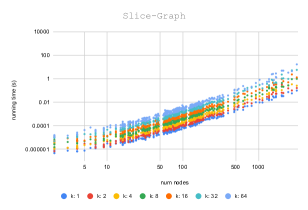
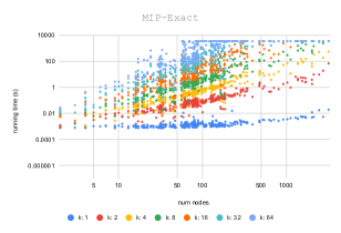
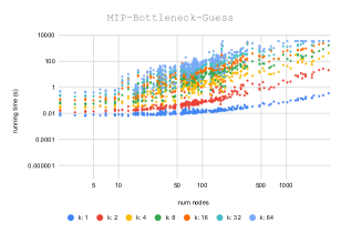
Figure 4: Running times of SliceGraph and different MIP lower bound solves across the production models, where data points are colored by $k\in\{1,2,4,8,16,32,64\}$: (left) one call to SliceGraph, (middle) exact MIP solves, (right) guess-the-bottleneck MIP formulation.

Table 1: Geometric means of the approximation ratio upper bounds $\textnormal{{SliceGraph}}(G,k,\pi)/L(G,k)$ across production models. Compares different topological ordering heuristics relative to the simple combinatorial lower bound in Lemma 4.2.

Algorithm	$k=2$	$k=4$	$k=8$	$k=16$	$k=32$	$k=64$
mla	1.216	1.538	1.950	2.224	2.304	2.326
mla-weighted	1.206	1.516	1.920	2.182	2.258	2.283
random-1	1.220	1.551	1.959	2.230	2.309	2.333
random-100	1.201	1.512	1.916	2.179	2.258	2.282
random-10000	1.199	1.509	1.911	2.176	2.256	2.281
brkga-100	1.201	1.516	1.919	2.184	2.263	2.288
brkga-10000	1.199	1.509	1.910	2.175	2.255	2.272

Table 2: Geometric means of the MIP lower bound improvements relative to Lemma 4.2 across the production models. Unsolved MIPs use the best objective value found before the time limit. The percent of instances whose best objective value is greater than or equal to the simple lower bound is given in parenthesis.

Lower bound	$k=2$	$k=4$	$k=8$	$k=16$	$k=32$	$k=64$
bottleneck-no-dag	1.002 (100)	1.002 (100)	1.004 (100)	1.006 (100)	1.005 (100)	1.002 (100)
bottleneck-no-cut-io	1.006 (100)	1.003 (100)	1.007 (100)	1.007 (100)	1.005 (100)	1.004 (100)
bottleneck	1.150 (99.7)	1.193 (99.7)	1.238 (99.7)	1.255 (99.7)	1.260 (99.7)	1.259 (99.7)
guess-the-bottleneck	1.187 (100)	1.274 (99.1)	1.260 (99.1)	1.253 (98.3)	1.252 (95.9)	1.244 (92.6)
exact	1.187 (100)	1.468 (100)	1.829 (100)	2.050 (100)	1.938 (95.1)	1.689 (79.1)

Table 3: Geometric means of the improved approximation ratio upper bounds across the production models using brkga-10000 and the best available lower bound from the MIP hierarchy.

Lower bound	$k=2$	$k=4$	$k=8$	$k=16$	$k=32$	$k=64$
simple (Lemma 4.2)	1.199	1.509	1.910	2.175	2.255	2.272
bottleneck	1.042	1.264	1.543	1.733	1.789	1.804
guess-the-bottleneck	1.010	1.184	1.515	1.730	1.788	1.804
exact	1.010	1.027	1.043	1.058	1.143	1.270

Random

The $\texttt{random-}T$ algorithm samples $T$ i.i.d. node weight vectors $\mathbf{x}^{(t)}\in[0,1]^{n}$ where $x^{(t)}_{i}\sim U(0,1)$, maps them to topological orders $\pi^{(t)}$ as described in Section 3.3, and returns $\min_{t\in[T]}\textnormal{{SliceGraph}}(G,\pi^{(t)},k)$.

BRKGA

The brkga-100 entries in Table 1 run BRKGA with Algorithm 2 and $(p,g)=(10,10)$, where $p$ is the population size and $g$ is the number of generations, to get $100$ total candidate evaluations. The brkga-10000 entries set $(p,g)=(100,100)$ for $10^{4}$ candidate evaluations. Note that BRKGA requires some “warm starting” since brkga-100 underperforms random-100, but improves in the long run.

MLA

A minimum linear arrangement (MLA) of an undirected graph $G=(V,E,w)$ is a node permutation $\pi\in\mathfrak{S}_{V}$ minimizing the objective

$$h(\pi)=\sum_{\{u,v\}\in E}w(u,v)\cdot\left\lvert\pi^{-1}(u)-\pi^{-1}(v)\right\rvert.$$

To generalize this idea to computation graphs, we restrict the search by taking $h(\pi)=\infty$ if $\pi$ is not a topological order, and setting $w(u,v)=1$ for the (unweighted) mla objective or $w(u,v)=\textnormal{{io}}(u,v)$ for mla-weighted in Table 1.

MLA is also an NP-hard problem, so we again use BRKGA to optimize this objective (similar to Algorithm 2), but now the fitness is $h(\pi(\mathbf{x}))$. We set $(p,g)=(100,100)$ for $10^{4}$ total candidate evaluations. Table 1 demonstrates that there is a clear benefit to using mla-weighted over mla for MTPP, which agrees with intuition. Even though MLA orderings optimize for a different objective, they are still very competitive, especially for being a zero-shot heuristic.

5.4 MIP lower bounds and tighter approximation ratios

Now we compare our MIP-based lower bounds to the simple combinatorial lower bound in Lemma 4.2. We solve different bottleneck formulations for each graph and report the geometric means of these improvements $\text{LB}(G,k)/L(G,k)$ in Table 2. The first two rows are relaxations of the three-superblock formulation: bottleneck-no-dag is the bottleneck MIP in Section 4.2 without any DAG constraints, and bottleneck-no-io is the bottleneck MIP without any tensor edge-cut costs. Both relaxations are weak in isolation, but when combined to get bottleneck from Section 4.2 we start making progress. Note that solving the exact MIP (Figure 3) is too slow to be a general-purpose graph partitioning algorithm inside an ML compiler, but it does allow us to certify how well an algorithm performs offline. See Figure 4 for a comparison of running times.

Finally, we take the best partitioning results brkga-10000 and our improved lower bounds to show how the approximation guarantees get tighter as we strengthen the MIP formulations. We sort the rows of Table 3 in increasing order of solve complexity (i.e., our MIP lower bound hierarchy), and for each row we consider the best per-instance lower bound computed so far, hence the monotonic improvement even though the exact solves struggle to optimally partition graphs for $k\geq 32$ in Table 2. We highlight the improvement in the geometric means of approximation ratios from row 1 to row 4 of Table 3. Prior to our work, the reason for the large approximation ratio upper bounds in the first row was unclear—is the simple combinatorial lower bound weak, or can the partitioning algorithms be improved? As a final data point, for $k\leq 16$ we are provably within $5.8\%$ of optimal compared to the initial $2.175$-approximation.

6 Related work

Model parallelism

Two of the seminal works on pipeline parallelism for machine learning are GPipe (Huang et al., 2019) and PipeDream (Narayanan et al., 2019; 2021). These papers focus on scaling up DNN training and have spawned a long list of related work: torchgpipe (Kim et al., 2020), FPDeep (Wang et al., 2020), HetPipe (Park et al., 2020), Pipemare (Yang et al., 2021), TeraPipe (Li et al., 2021), BaPipe (Zhao et al., 2022), SAPipe (Chen et al., 2022), synchronous pipeline planning in (Luo et al., 2022), BPipe (Kim et al., 2023), and breadth-first pipeline parallelism (Lamy-Poirier, 2023).

Of these works, PipeDream studies the most similar mathematical model (Narayanan et al., 2019, Section 3.1). There is some overlap with MTPP (e.g., a min-max running time objective), but there are also major differences:

1. PipeDream assumes a single topological order, and that the induced quotient graph is a path graph. This means IO can only flow between adjacent blocks instead of to shared memory for downstream consumers.

2. PipeDream uses communication-work concurrency, so the running time of a processor executing ops $S\subseteq V$ is $\max(\textnormal{{work}}(S),\textnormal{{io}}(V\setminus S,S)+\textnormal{{io}}(S,V\setminus S))$.

3. PipeDream supports data parallelism and is designed to use replicated workers. The model weight updates for replicated workers use weight stashing and a vertical sync technique, but this is not necessary for inference.

Tensor sharding is another technique to push beyond data parallelism, e.g., Mesh TensorFlow (Shazeer et al., 2018), Megatron-LM (Shoeybi et al., 2019), and GSPMD (Xu et al., 2021). For inference workloads, there have also been major advances in scaling up transformers (Zhai et al., 2022, Liu et al., 2022, Pope et al., 2022) and model partitioning using reinforcement learning (Xie et al., 2022).

Acyclic graph partitioning

Acyclic graph partitioning has its origins in multiprocessor scheduling (Garey & Johnson, 1979). Since then, there have been several notable applications of acyclic partitioning for pipeline parallelism (Cong et al., 1994, Gordon et al., 2006, Sanchez et al., 2011). The computational hardness and inapproximability of balanced acyclic partitioning has recently been revisited in (Moreira et al., 2017, Papp et al., 2023). Some practical approaches for acyclic graph partitioning leverage multilevel algorithms with graph coarsening (Moreira et al., 2020, Herrmann et al., 2019, Popp et al., 2021) and integer programming formulations with branch-and-bound algorithms (Nossack & Pesch, 2014, Albareda-Sambola et al., 2019, Özkaya & Çatalyürek, 2022).

7 Conclusion

This work presents fast and effective pipeline partitioning algorithms for maximizing inference throughput. Our exact MIP formulation and its sparse relaxations in Section 4 allow us to give strong a posteriori approximation guarantees for MTPP in practice, which can be invaluable since countless software engineering hours are spent partitioning mission-critical models across ML accelerators to improve system efficiency. Without tight lower bounds, it is often unclear if practitioners should continue searching for better partitions, or if they are already close to optimal but don’t know it. Our MIP formulations enable us to compute certificates that can act as a stopping condition on further investment of software engineering time.

Our experiments on production models in Section 5 show that SliceGraph algorithms are sufficiently effective, and that further effort on MTPP in practice would be better spent improving the cost models that provide the node weights we feed into partitioning algorithms. On the theoretical side, we pose two exciting open questions for future research: (1) is there a constant-factor approximation algorithm for MTPP, and (2) what are the integrality gaps of the bottleneck MIP relaxations in Section 4?

Appendix A Missing algorithms and analysis for Section 3

A.1 Main results

See 3.3

Proof.

For any topological order $\pi\in\mathfrak{S}_{V}$, initialize segment_cost for $G(\pi)$ in $O(n^{2}+m\log^{2}(n))$ time and $O(n^{2})$ space by Lemma 3.2. Then, run the dynamic programming algorithm $\textnormal{{DP}}(\texttt{segment\_cost},n,k)$ on the full topological order $\pi$, which can be done in $O(n^{2}k)$ time and $O(n^{2})$ space since there are $O(nk)$ states and each state can be computed recursively in $O(n)$ time after preprocessing all $[\ell,r]$ segment costs. This gives an optimal stars-and-bars partition of $\pi$ into $k$ (possibly empty) blocks for the MTPP objective in Eq. Equation 4, which proves the result. ∎

See 3.5

Proof.

Consider a graph with $n=2k$ nodes of two types: nodes $\{1,2,\dots,k\}$ are heavy with weight $\textnormal{{work}}(v_{i})=1-\varepsilon$, and nodes $\{k+1,k+2,\dots,2k\}$ are light with weight $\textnormal{{work}}(v_{i})=\varepsilon$. Add one directed edge $(1,k+1)$ with weight $10k$. Clearly $\textnormal{OPT}=1$ since $G$ can be partitioned as $P^{*}=\{\{1,k+1\},\{2,k+2\},\dots,\{k,2k\}\}$, which means $f(P_{i}^{*})=(1-\varepsilon)+\varepsilon=1$ for all $i\in[k]$ since each block has no incoming or outgoing edges.

Now consider the topological order $\pi=(1,2,\dots,k,2k,2k-1,\dots,k+1)$. Any stars-and-bars partition $P$ with an internal separator must cut the edge $(1,k+1)$, which means $\max_{i\in[k]}\{f(P_{i})\}\geq 10k$. Therefore, the optimal slicing of $\pi$ groups all nodes into the same block and has objective value $k(1-\varepsilon)+k\varepsilon=k$. ∎

Remark A.1.

Going a step further, consider graph $G$ above without edge $(1,k+1)$. Any topological sort-based algorithm for $k$ blocks can be as bad as $\frac{2k}{k+1}\cdot\textnormal{OPT}$ since any stars-and-bars partition must have an MTPP objective value of at least $\max\{2(1-\varepsilon),(1-\varepsilon)+k\varepsilon\}$. To see this, observe that either two heavy nodes must be in the same block or there is a divider between each pair of adjacent heavy nodes. Setting $\varepsilon=\frac{1}{k+1}$ proves the claim.

A.2 Kahn’s topological sort algorithm with node priorities

Algorithm 3 Kahn’s topological sort algorithm with tie-breaking by node priorities.

1:function KahnWithNodePriorities(graph $G=(V,E)$, node priorities $\mathbf{x}\in[0,1]^{n}$)

2:     Initialize $\pi\leftarrow\mathbf{0}_{n}$ and $\texttt{indegree}\leftarrow\mathbf{0}_{n}$

3:     for each $v\in V$ do

4:         $\texttt{indegree}[v]\leftarrow|N^{-}(v)|$      

5:     Initialize priority queue $q$ +++ // Max heap implementation

6:     for each leaf node $v\in V$ do

7:         Insert priority-node pair $(x_{v},v)$ into $q$      

8:     Initialize index $i\leftarrow 1$

9:     while $q$ is not empty do

10:         $u\leftarrow\text{top}(q)$; $\text{pop}(q)$

11:         $\pi[i]\leftarrow u$

12:         for each $v\in N^{+}(u)$ do

13:              $\texttt{indegree}[v]\leftarrow\texttt{indegree}[v]-1$

14:              if $\texttt{indegree}[v]=0$ then

15:                  Insert priority-node pair $(x_{v},v)$ into $q$                        

16:         $i\leftarrow i+1$      

17:     return $\pi$

A.3 Segment cost data structure

We start with a simpler version of the segment cost data structure that makes entrywise updates to the io_struct[][] array during initialization. We give a proof of its correctness, and then we explain how to speed up this preprocessing step using a two-dimensional Fenwick tree to achieve faster $O(\log^{2}(n))$ subrectangle updates (Mishra, 2013).

Warmup A.2.

There is a SegmentCostDataStructure that takes a computation graph $G=(V,E)$ and topological order $\pi\in\mathfrak{S}_{V}$ as input, and supports the following operations:

• $\textnormal{{Initialize}}(G,\pi)$: Preprocesses the graph in $O(n^{3})$ time.

• $\textnormal{{Query}}(\ell,r)$: Returns $f(\{v_{\pi(\ell)},\dots,v_{\pi(r)}\})$ in Eq. Section 2.2 in constant time, after initialization.

Proof.

The correctness is clear by inspection since we are memoizing the contributions of work, io, and $\texttt{size}_{\texttt{param}}$ to the overall cost of each segment. Calls to $\textnormal{{Query}}(\ell,r)$ take constant time since we are only performing $O(1)$ array look-ups and arithmetic operations. It remains to show that the memoization data structures can be built in $O(mn^{2})$ time.

The prefix-sum data structures work_struct and mem_struct can all be built in $O(n)$ time since we take one pass over each vertex of the computation graph, and updating each entry requires $O(1)$ time (assuming $O(1)$-time queries to work and $\texttt{size}_{\texttt{param}}$). Furthermore, io_struct can be constructed in $O(n^{3})$ time. To see this, observe that we take a single pass over all vertices $u\in V$, and for each vertex, we perform at most $O(n^{2})$ arithmetic operations and calls to $\texttt{size}_{\texttt{out}}$ since each update is for a distinct $[\ell,r]$ interval. ∎

Algorithm 4 Segment cost data structure for blocks of the form $P=\{v_{\pi(\ell)},v_{\pi(\ell+1)},\dots,v_{\pi(r)}\}$.

1:function Initialize($G$, $\pi$)

2:     $\texttt{work\_struct}\leftarrow\texttt{InitWorkStruct}(G,\pi)$

3:     $\texttt{mem\_struct}\leftarrow\texttt{InitMemStruct}(G,\pi)$

4:     $\texttt{io\_struct}\leftarrow\texttt{InitIOStruct}(G,\pi)$

5:function Query($\ell$, $r$)

6:     Query $\textnormal{{work}}\leftarrow\texttt{work\_struct}[r]-\texttt{work\_struct}[\ell-1]$

7:     Query $\texttt{size}_{\texttt{param}}\leftarrow\texttt{mem\_struct}[r]-\texttt{mem\_struct}[\ell-1]$

8:     Set $\texttt{overflow}\leftarrow\texttt{size}_{\texttt{param}}+\texttt{peak}([v_{\pi(\ell)},v_{\pi(\ell+1)},\dots,v_{\pi(r)}])-M$

9:     Update $\texttt{overflow}\leftarrow\frac{1}{B}\max\left\{\texttt{overflow},0\right\}$

10:     Query $\textnormal{{io}}\leftarrow\texttt{io\_struct}[\ell][r]$

11:     return $\textnormal{{work}}+\texttt{overflow}+\textnormal{{io}}$

In the Algorithm 5 pseudocode, we use the fact that $\pi\in\mathfrak{S}_{V}$ is a permutation of the vertices and that $\pi^{-1}:V\rightarrow[n]$ tells us the index at which a given node appears in the topological order.

Now we explain how the preprocessing running time can be reduced using subrectangle range updates to subtract $\texttt{size}_{\texttt{out}}(u)$ from disjoint regions of the two-dimensional io_struct[][] array.

Algorithm 5 Segment cost data structure helper functions.

1:function InitWorkStruct($G$, $\pi$)

2:// Builds 1D array of work prefix sums

3:     Initialize $\texttt{work\_struct}\leftarrow\mathbf{0}_{n}$

4:     $\texttt{work\_struct}[1]\leftarrow\textnormal{{work}}(\pi(1))$

5:     for $i=2$ to $n$ do

6:         $\texttt{work\_struct}[i]\leftarrow\texttt{work\_struct}[i-1]+\textnormal{{work}}(\pi(i))$      

7:     return work_struct

8:function InitMemStruct($G$, $\pi$)

9:// Builds 1D array of $\texttt{size}_{\texttt{param}}$ prefix sums

10:     Initialize $\texttt{mem\_struct}\leftarrow\mathbf{0}_{n}$

11:     $\texttt{mem\_struct}[1]\leftarrow\texttt{size}_{\texttt{param}}(\pi(1))$

12:     for $i=2$ to $n$ do

13:         $\texttt{mem\_struct}[i]\leftarrow\texttt{mem\_struct}[i-1]+\texttt{size}_{\texttt{param}}(\pi(i))$      

14:     return mem_struct

15:function InitIOStruct($G$, $\pi$)

16:// Builds 2D array of io segment costs

17:     Compute $\texttt{total}\leftarrow\sum_{v\in V}\texttt{size}_{\texttt{out}}(v)$

18:     Initialize $n\times n$ array io_struct with total

19:     for $u\in V$ do +++ // Remove $\texttt{size}_{\texttt{out}}(u)$ from eligible segments

20:         Let $S=(v_{1},v_{2},\dots,v_{d})$ be the nodes in $\{u\}\cup N^{+}(u)$ sorted s.t. $\pi^{-1}(v_{i})<\pi^{-1}(v_{i+1})$

21:         for $1\leq\ell\leq r<\pi^{-1}(v_{1})$ do

22:              $\texttt{io\_struct}[\ell][r]\leftarrow\texttt{io\_struct}[\ell][r]-\texttt{size}_{\texttt{out}}(u)$          

23:         for $i=1$ to $d-1$ do

24:              for $\pi^{-1}(v_{i})<\ell\leq r<\pi^{-1}(v_{i+1})$ do

25:                  $\texttt{io\_struct}[\ell][r]\leftarrow\texttt{io\_struct}[\ell][r]-\texttt{size}_{\texttt{out}}(u)$                        

26:         for $\pi^{-1}(v_{d})<\ell\leq r\leq n$ do

27:              $\texttt{io\_struct}[\ell][r]\leftarrow\texttt{io\_struct}[\ell][r]-\texttt{size}_{\texttt{out}}(u)$          

28:         for $1\leq\ell\leq\pi^{-1}(v_{1})$ do +++ // Segments fully containing $\{v_{1},v_{d}\}$

29:              for $\pi^{-1}(v_{d})\leq r\leq n$ do

30:                  $\texttt{io\_struct}[\ell][r]\leftarrow\texttt{io\_struct}[\ell][r]-\texttt{size}_{\texttt{out}}(u)$                             

31:     return io_struct

See 3.2

Proof.

We use a two-dimensional Fenwick tree (Mishra, 2013) to implement the io_struct array. This data structure needs $O(n^{2})$ time and space to initialize as $\mathbf{0}_{n\times n}$. It also supports the operation $\texttt{Update}(p,q,x)$ where $p=(i_{1},j_{1})$ and $q=(i_{2},j_{2})$ define two corners of a rectangular sub-array, and adds $x$ to all entries $\texttt{io\_struct}[i][j]$ for all $(i,j)\in[i_{1},i_{2}]\times[j_{1},j_{2}]$ in time $O(\log^{2}(n))$. Therefore, we can first initialize all entries to total in $O(\log^{2}(n))$ time.

For each $u\in V$, we describe how to update io_struct in $O(\deg^{+}(u)\log^{2}(n))$ time. First, observe that there are $\deg^{+}(u)+2$ updates in Lines 17–24 of the form $i\leq\ell\leq r\leq j$. It follows that we can call $\texttt{Update}((\ell,\ell),(r,r),-\texttt{size}_{\texttt{out}}(u))$ to correctly update the Fenwick tree. Note that this updates entries that will never be queried (i.e., when $\ell>r$), but this is not a problem. Finally, we call $\texttt{Update}((1,\pi^{-1}(u)),(\pi^{-1}(v_{d}),n),-\texttt{size}_{\texttt{out}}(u))$ to update segments that fully contain $\{u,v_{d}\}$. Putting everything together, the total running time to maintain io_struct as a two-dimensional Fenwick tree is

$$O\left(n^{2}\right)+\sum_{u\in V}O\left(\deg^{+}(u)\log^{2}(n)\right)=O\left(n^{2}+m\log^{2}(n)\right).$$

Since each element-wise query takes $O(\log^{2}(n))$ time in isolation, we use the fact that we can iterate over all $O(n^{2})$ entries of the Fenwick tree and write the values of $\texttt{io\_struct}[\ell][r]$ in a separate two-dimensional array in amortized $O(n^{2})$ time. This allows us to achieve $O(1)$ time queries for the segment cost data structure after initialization. Correctness follows from Mishra (2013) and A.2. ∎

Appendix B Additional experiments and details for Section 5

B.1 REGAL graphs

We describe the synthetic computation graph constructions in Paliwal et al. (2020, Appendix A.1.4). The base graphs are first sampled from a set of classic random graph model (see Table 2 therein for the parameters of each random graph model). The graphs have $50\leq n\leq 200$ nodes, and are converted to directed acyclic graphs via a random topological order. The size of each tensor is sampled from the normal distribution $\mathcal{N}(50,10)$, and each node cost is the sum of its input and output tensor costs plus a random fraction $r$ of the total memory cost (i.e., the sum of all tensor sizes), where $r\sim\mathcal{N}(0,0.1)$. If a node has more than one output tensor, we only use the lexicographically least according to the tensor index. Finally, Paliwal et al. (2020) filter these graphs and only keep those that are sufficiently hard for their min-peak scheduling objective.

B.2 REGAL results

We present a parallel set of results to accompany our running time plots and tables of approximation ratio upper bounds for the production dataset in Section 5.

Table 4: Geometric means of the approximation ratio upper bounds $\textnormal{{SliceGraph}}(G,k,\pi)/L(G,k)$ across REGAL graphs. Compares different topological ordering heuristics relative to the simple combinatorial lower bound in Lemma 4.2.

Algorithm	$k=2$	$k=4$	$k=8$	$k=16$	$k=32$	$k=64$
random-1	1.179	1.296	1.406	1.849	2.551	3.025
random-100	1.125	1.240	1.344	1.791	2.501	3.010
random-10000	1.099	1.208	1.315	1.763	2.478	3.004
brkga-100	1.106	1.217	1.327	1.778	2.492	3.008
brkga-10000	1.044	1.137	1.264	1.718	2.447	2.998

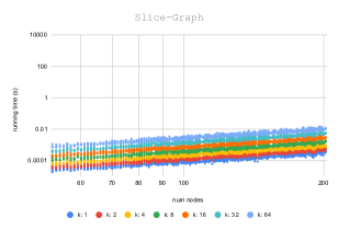
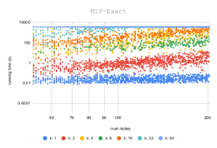
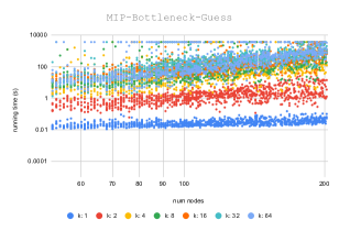
Figure 5: Running times of SliceGraph and different MIP lower bound solves across the REGAL models, where data points are colored by $k\in\{1,2,4,8,16,32,64\}$: (left) one call to SliceGraph, (middle) exact MIP solves, (right) guess-the-bottleneck MIP formulation.

Table 5: Geometric means of the MIP lower bound improvements relative to Lemma 4.2 across REGAL graphs. Unsolved MIPs use the best objective value found before the time limit. The percent of instances whose best objective value is greater than or equal to the simple lower bound is given in parenthesis.

Lower bound	$k=2$	$k=4$	$k=8$	$k=16$	$k=32$	$k=64$
bottleneck-no-dag	1.000 (100)	1.000 (100)	1.000 (100)	1.000 (100)	1.000 (100)	1.000 (100)
bottleneck-no-io	1.000 (100)	1.000 (100)	1.000 (100)	1.000 (100)	1.000 (100)	1.000 (100)
bottleneck	1.021 (100)	1.002 (100)	1.000 (100)	1.000 (100)	1.000 (100)	1.000 (100)
bottleneck-guess	1.023 (100)	1.003 (95.1)	1.000 (94.1)	1.000 (96.7)	1.000 (97.6)	1.000 (88.6)
exact	1.023 (100)	1.089 (100)	1.189 (100)	1.533 (100)	1.445 (97.8)	1.141 (42.0)

Table 6: Geometric means of the improved approximation ratio upper bounds across REGAL graphs using brkga-10000 and the best available lower bound from the MIP hierarchy.

Lower bound	$k=2$	$k=4$	$k=8$	$k=16$	$k=32$	$k=64$
simple (Lemma 4.2)	1.044	1.137	1.264	1.718	2.447	2.998
bottleneck	1.021	1.134	1.263	1.717	2.445	2.996
bottleneck-guess	1.020	1.133	1.263	1.717	2.445	2.996
exact	1.020	1.044	1.063	1.120	1.692	2.625

B.3 Solving the MIPs

To solve the MIPs that underpin Table 2 and Table 5, we used a combination of the Gurobi (Gurobi Optimization, LLC, 2023) and SCIP (Bestuzheva et al., 2021) solvers. For bottleneck-no-dag, bottleneck-no-cut-io and bottleneck, we used Gurobi with a 15-minute time limit, and for exact we relaxed that to 60 minutes because these MIPs are tougher to solve. For technical reasons having to do with our computing setup, we instead used SCIP for guess-the-bottleneck, with a 60-minute time budget that was shared across all values of $k$ of the MIPs that compose a single guess-the-bottleneck instance (one MIP per guess). A non-trivial fraction of the instances failed to solve to provable optimality within the time limit, especially for exact with $k=64$. In these cases, the solver still returns a valid lower bound, and we use that.

References

- Abadi et al. (2016) Abadi, M., Barham, P., Chen, J., Chen, Z., Davis, A., Dean, J., Devin, M., Ghemawat, S., Irving, G., Isard, M., et al. TensorFlow: A system for large-scale machine learning. In 12th USENIX Symposium on Operating Systems Design and Implementation, pp. 265–283, 2016.
- Ahn et al. (2020) Ahn, B. H., Lee, J., Lin, J. M., Cheng, H.-P., Hou, J., and Esmaeilzadeh, H. Ordering chaos: Memory-aware scheduling of irregularly wired neural networks for edge devices. Proceedings of Machine Learning and Systems, 2:44–57, 2020.
- Albareda-Sambola et al. (2019) Albareda-Sambola, M., Marín, A., and Rodríguez-Chía, A. M. Reformulated acyclic partitioning for rail-rail containers transshipment. European Journal of Operational Research, 277(1):153–165, 2019.
- Bestuzheva et al. (2021) Bestuzheva, K., Besançon, M., Chen, W.-K., Chmiela, A., Donkiewicz, T., van Doornmalen, J., Eifler, L., Gaul, O., Gamrath, G., Gleixner, A., Gottwald, L., Graczyk, C., Halbig, K., Hoen, A., Hojny, C., van der Hulst, R., Koch, T., Lübbecke, M., Maher, S. J., Matter, F., Mühmer, E., Müller, B., Pfetsch, M. E., Rehfeldt, D., Schlein, S., Schlösser, F., Serrano, F., Shinano, Y., Sofranac, B., Turner, M., Vigerske, S., Wegscheider, F., Wellner, P., Weninger, D., and Witzig, J. The SCIP Optimization Suite 8.0. Technical report, Optimization Online, December 2021. URL http://www.optimization-online.org/DB_HTML/2021/12/8728.html.
- Bhakta et al. (2017) Bhakta, P., Cousins, B., Fahrbach, M., and Randall, D. Approximately sampling elements with fixed rank in graded posets. In Proceedings of the Twenty-Eighth Annual ACM-SIAM Symposium on Discrete Algorithms, pp. 1828–1838. SIAM, 2017.
- Bubley & Dyer (1999) Bubley, R. and Dyer, M. Faster random generation of linear extensions. Discrete Mathematics, 201(1):81–88, 1999.
- Chen et al. (2015) Chen, T., Li, M., Li, Y., Lin, M., Wang, N., Wang, M., Xiao, T., Xu, B., Zhang, C., and Zhang, Z. MXNet: A flexible and efficient machine learning library for heterogeneous distributed systems. arXiv preprint arXiv:1512.01274, 2015.
- Chen et al. (2022) Chen, Y., Xie, C., Ma, M., Gu, J., Peng, Y., Lin, H., Wu, C., and Zhu, Y. SAPipe: Staleness-aware pipeline for data parallel DNN training. In Advances in Neural Information Processing Systems, 2022.
- Cong et al. (1994) Cong, J., Li, Z., and Bagrodia, R. Acyclic multi-way partitioning of boolean networks. In Proceedings of the 31st annual design automation conference, pp. 670–675, 1994.
- Dao et al. (2022) Dao, T., Fu, D., Ermon, S., Rudra, A., and Ré, C. FlashAttention: Fast and memory-efficient exact attention with IO-awareness. Advances in Neural Information Processing Systems, 35:16344–16359, 2022.
- Dasari et al. (2021) Dasari, U. K., Temam, O., Narayanaswami, R., and Woo, D. H. Apparatus and mechanism for processing neural network tasks using a single chip package with multiple identical dies, March 2 2021. US Patent 10,936,942.
- Gao et al. (2020) Gao, Y., Liu, Y., Zhang, H., Li, Z., Zhu, Y., Lin, H., and Yang, M. Estimating GPU memory consumption of deep learning models. In Proceedings of the 28th ACM Joint Meeting on European Software Engineering Conference and Symposium on the Foundations of Software Engineering, pp. 1342–1352, 2020.
- García-Segador & Miranda (2019) García-Segador, P. and Miranda, P. Bottom-up: A new algorithm to generate random linear extensions of a poset. Order, 36(3):437–462, 2019.
- Garey & Johnson (1979) Garey, M. R. and Johnson, D. S. Computers and Intractability. W. H. Freeman, 1979.
- Gonçalves & Resende (2011) Gonçalves, J. F. and Resende, M. G. Biased random-key genetic algorithms for combinatorial optimization. Journal of Heuristics, 17(5):487–525, 2011.
- Gordon et al. (2006) Gordon, M. I., Thies, W., and Amarasinghe, S. Exploiting coarse-grained task, data, and pipeline parallelism in stream programs. ACM SIGPLAN Notices, 41(11):151–162, 2006.
- Gurobi Optimization, LLC (2023) Gurobi Optimization, LLC. Gurobi Optimizer Reference Manual, 2023. URL https://www.gurobi.com.
- Herrmann et al. (2019) Herrmann, J., Ozkaya, M. Y., Uçar, B., Kaya, K., and Çatalyürek, Ü. V. V. Multilevel algorithms for acyclic partitioning of directed acyclic graphs. SIAM Journal on Scientific Computing, 41(4):A2117–A2145, 2019.
- Hochbaum & Shmoys (1987) Hochbaum, D. S. and Shmoys, D. B. Using dual approximation algorithms for scheduling problems theoretical and practical results. Journal of the ACM, 34(1):144–162, 1987.
- Huang et al. (2019) Huang, Y., Cheng, Y., Bapna, A., Firat, O., Chen, D., Chen, M., Lee, H., Ngiam, J., Le, Q. V., Wu, Y., et al. GPipe: Efficient training of giant neural networks using pipeline parallelism. Advances in Neural Information Processing Systems, 32, 2019.
- Huber (2006) Huber, M. Fast perfect sampling from linear extensions. Discrete Mathematics, 306(4):420–428, 2006.
- Jouppi et al. (2017) Jouppi, N. P., Young, C., Patil, N., Patterson, D., Agrawal, G., Bajwa, R., Bates, S., Bhatia, S., Boden, N., Borchers, A., et al. In-datacenter performance analysis of a tensor processing unit. In Proceedings of the 44th Annual International Symposium on Computer Architecture, pp. 1–12, 2017.
- Jouppi et al. (2023) Jouppi, N. P., Kurian, G., Li, S., Ma, P., Nagarajan, R., Nai, L., Patil, N., Subramanian, S., Swing, A., Towles, B., et al. TPU v4: An optically reconfigurable supercomputer for machine learning with hardware support for embeddings. arXiv preprint arXiv:2304.01433, 2023.
- Kahn (1962) Kahn, A. B. Topological sorting of large networks. Communications of the ACM, 5(11):558–562, 1962.
- Karzanov & Khachiyan (1991) Karzanov, A. and Khachiyan, L. On the conductance of order Markov chains. Order, 8:7–15, 1991.
- Kaufman et al. (2021) Kaufman, S., Phothilimthana, P., Zhou, Y., Mendis, C., Roy, S., Sabne, A., and Burrows, M. A learned performance model for tensor processing units. Proceedings of Machine Learning and Systems, 3:387–400, 2021.
- Kim et al. (2020) Kim, C., Lee, H., Jeong, M., Baek, W., Yoon, B., Kim, I., Lim, S., and Kim, S. torchgpipe: On-the-fly pipeline parallelism for training giant models. arXiv preprint arXiv:2004.09910, 2020.
- Kim et al. (2023) Kim, T., Kim, H., Yu, G.-I., and Chun, B.-G. BPipe: Memory-balanced pipeline parallelism for training large language models. International Conference on Machine Learning, pp. 16639–16653, 2023.
- Lamy-Poirier (2023) Lamy-Poirier, J. Breadth-first pipeline parallelism. Proceedings of Machine Learning and Systems, 5, 2023.
- Lattner et al. (2021) Lattner, C., Amini, M., Bondhugula, U., Cohen, A., Davis, A., Pienaar, J., Riddle, R., Shpeisman, T., Vasilache, N., and Zinenko, O. MLIR: Scaling compiler infrastructure for domain specific computation. In 2021 IEEE/ACM International Symposium on Code Generation and Optimization (CGO), pp. 2–14. IEEE, 2021.
- Li et al. (2021) Li, Z., Zhuang, S., Guo, S., Zhuo, D., Zhang, H., Song, D., and Stoica, I. Terapipe: Token-level pipeline parallelism for training large-scale language models. In International Conference on Machine Learning, pp. 6543–6552. PMLR, 2021.
- Lin et al. (2021) Lin, J., Chen, W.-M., Cai, H., Gan, C., and Han, S. Mcunetv2: Memory-efficient patch-based inference for tiny deep learning. arXiv preprint arXiv:2110.15352, 2021.
- Liu et al. (2022) Liu, Z., Hu, H., Lin, Y., Yao, Z., Xie, Z., Wei, Y., Ning, J., Cao, Y., Zhang, Z., Dong, L., et al. Swin transformer v2: Scaling up capacity and resolution. In Proceedings of the IEEE/CVF conference on computer vision and pattern recognition, pp. 12009–12019, 2022.
- Luo et al. (2022) Luo, Z., Yi, X., Long, G., Fan, S., Wu, C., Yang, J., and Lin, W. Efficient pipeline planning for expedited distributed DNN training. In IEEE INFOCOM 2022-IEEE Conference on Computer Communications, pp. 340–349. IEEE, 2022.
- Marchal et al. (2019) Marchal, L., Simon, B., and Vivien, F. Limiting the memory footprint when dynamically scheduling DAGs on shared-memory platforms. Journal of Parallel and Distributed Computing, 128:30–42, 2019.
- Matthews (1991) Matthews, P. Generating a random linear extension of a partial order. The Annals of Probability, 19(3):1367–1392, 1991.
- Mei & Chu (2016) Mei, X. and Chu, X. Dissecting GPU memory hierarchy through microbenchmarking. IEEE Transactions on Parallel and Distributed Systems, 28(1):72–86, 2016.
- Mishra (2013) Mishra, P. A new algorithm for updating and querying sub-arrays of multidimensional arrays. arXiv preprint arXiv:1311.6093, 2013.
- Moreira et al. (2017) Moreira, O., Popp, M., and Schulz, C. Graph partitioning with acyclicity constraints. In 16th International Symposium on Experimental Algorithms (SEA), volume 75, pp. 30:1–30:15, 2017.
- Moreira et al. (2020) Moreira, O., Popp, M., and Schulz, C. Evolutionary multi-level acyclic graph partitioning. Journal of Heuristics, 26(5):771–799, 2020.
- Narayanan et al. (2019) Narayanan, D., Harlap, A., Phanishayee, A., Seshadri, V., Devanur, N. R., Ganger, G. R., Gibbons, P. B., and Zaharia, M. PipeDream: Generalized pipeline parallelism for DNN training. In Proceedings of the 27th ACM Symposium on Operating Systems Principles, pp. 1–15, 2019.
- Narayanan et al. (2021) Narayanan, D., Phanishayee, A., Shi, K., Chen, X., and Zaharia, M. Memory-efficient pipeline-parallel DNN training. In International Conference on Machine Learning, pp. 7937–7947. PMLR, 2021.
- Nossack & Pesch (2014) Nossack, J. and Pesch, E. A branch-and-bound algorithm for the acyclic partitioning problem. Computers & Operations Research, 41:174–184, 2014.
- Özkaya & Çatalyürek (2022) Özkaya, M. Y. and Çatalyürek, Ü. V. A simple and elegant mathematical formulation for the acyclic DAG partitioning problem. arXiv preprint arXiv:2207.13638, 2022.
- Paliwal et al. (2020) Paliwal, A., Gimeno, F., Nair, V., Li, Y., Lubin, M., Kohli, P., and Vinyals, O. Reinforced genetic algorithm learning for optimizing computation graphs. In Proceedings of the 8th International Conference on Learning Representations (ICLR), 2020.
- Papp et al. (2023) Papp, P. A., Anegg, G., and Yzelman, A.-J. N. Partitioning hypergraphs is hard: Models, inapproximability, and applications. In Proceedings of the 35th ACM Symposium on Parallelism in Algorithms and Architectures, pp. 415–425, 2023.
- Park et al. (2020) Park, J. H., Yun, G., Chang, M. Y., Nguyen, N. T., Lee, S., Choi, J., Noh, S. H., and Choi, Y.-r. HetPipe: Enabling large DNN training on (whimpy) heterogeneous GPU clusters through integration of pipelined model parallelism and data parallelism. In 2020 USENIX Annual Technical Conference (USENIX ATC 20), pp. 307–321, 2020.
- Paszke et al. (2019) Paszke, A., Gross, S., Massa, F., Lerer, A., Bradbury, J., Chanan, G., Killeen, T., Lin, Z., Gimelshein, N., Antiga, L., et al. PyTorch: An imperative style, high-performance deep learning library. Advances in Neural Information Processing Systems, 32, 2019.
- Pope et al. (2022) Pope, R., Douglas, S., Chowdhery, A., Devlin, J., Bradbury, J., Levskaya, A., Heek, J., Xiao, K., Agrawal, S., and Dean, J. Efficiently scaling transformer inference. arXiv preprint arXiv:2211.05102, 2022.
- Popp et al. (2021) Popp, M., Schlag, S., Schulz, C., and Seemaier, D. Multilevel acyclic hypergraph partitioning. In Proceedings of the Workshop on Algorithm Engineering and Experiments (ALENEX), pp. 1–15. SIAM, 2021.
- Sanchez et al. (2011) Sanchez, D., Lo, D., Yoo, R. M., Sugerman, J., and Kozyrakis, C. Dynamic fine-grain scheduling of pipeline parallelism. In 2011 International Conference on Parallel Architectures and Compilation Techniques, pp. 22–32. IEEE, 2011.
- Shazeer et al. (2018) Shazeer, N., Cheng, Y., Parmar, N., Tran, D., Vaswani, A., Koanantakool, P., Hawkins, P., Lee, H., Hong, M., Young, C., et al. Mesh-TensorFlow: Deep learning for supercomputers. Advances in Neural Information Processing Systems, 31, 2018.
- Shoeybi et al. (2019) Shoeybi, M., Patwary, M., Puri, R., LeGresley, P., Casper, J., and Catanzaro, B. Megatron-LM: Training multi-billion parameter language models using model parallelism. arXiv preprint arXiv:1909.08053, 2019.
- Vee et al. (2021) Vee, E. N., Purohit, M. D., Wang, J. R., Ravikumar, S., and Svitkina, Z. Scheduling operations on a computation graph, March 30 2021. US Patent 10,963,301.
- Wang et al. (2020) Wang, T., Geng, T., Li, A., Jin, X., and Herbordt, M. FPDeep: Scalable acceleration of cnn training on deeply-pipelined FPGA clusters. IEEE Transactions on Computers, 69(8):1143–1158, 2020.
- Wilson (2004) Wilson, D. B. Mixing times of lozenge tiling and card shuffling Markov chains. The Annals of Applied Probability, 14(1):274–325, 2004.
- Xie et al. (2022) Xie, X., Prabhu, P., Beaugnon, U., Phothilimthana, P., Roy, S., Mirhoseini, A., Brevdo, E., Laudon, J., and Zhou, Y. A transferable approach for partitioning machine learning models on multi-chip-modules. Proceedings of Machine Learning and Systems, 4:370–381, 2022.
- Xu et al. (2021) Xu, Y., Lee, H., Chen, D., Hechtman, B., Huang, Y., Joshi, R., Krikun, M., Lepikhin, D., Ly, A., Maggioni, M., et al. GSPMD: General and scalable parallelization for ML computation graphs. arXiv preprint arXiv:2105.04663, 2021.
- Yang et al. (2021) Yang, B., Zhang, J., Li, J., Ré, C., Aberger, C., and De Sa, C. Pipemare: Asynchronous pipeline parallel DNN training. Proceedings of Machine Learning and Systems, 3:269–296, 2021.
- Zhai et al. (2022) Zhai, X., Kolesnikov, A., Houlsby, N., and Beyer, L. Scaling vision transformers. In Proceedings of the IEEE/CVF Conference on Computer Vision and Pattern Recognition, pp. 12104–12113, 2022.
- Zhang et al. (2022) Zhang, K., Wang, H., Hu, H., Zou, S., Qiu, J., Li, T., and Wang, Z. TENSILE: A tensor granularity dynamic GPU memory scheduling method toward multiple dynamic workloads system. IEEE Transactions on Knowledge and Data Engineering, 2022.
- Zhao et al. (2022) Zhao, L., Xu, R., Wang, T., Tian, T., Wang, X., Wu, W., Ieong, C.-I., and Jin, X. Bapipe: Balanced pipeline parallelism for DNN training. Parallel Processing Letters, 32(03n04):2250005, 2022.