Long Range Voter Models and Dynamical Fractional Brownian Motion

Abstract.

We study the voter model on $\mathbb{Z}$ with long range interactions, as proposed by Hammond and Sheffield in [10]. We show the associated family of random walks converges to a one parameter family of evolving fractional Brownian motions. As a consequence we obtain that in equilibrium the voter model on $\mathbb{Z}$ with suitable long range interactions rescales to fractional Gaussian noise. The argument uses the Lindeberg swapping technique and heat kernel estimates for random walks with jump distributions in the domain of attraction of a stable law.

1. Introduction

1.1. Overview

For a law $\mu$ on $\mathbb{Z}$, we recall the voter model with interactions $\mu$. Suppose each site on $\mathbb{Z}$ is a voter who at time $t$ is affiliated to one of two political parties, either the $+1$ party or the $-1$ party. At time $t+1$ each voter will update their opinion by taking on the party affiliation of the voter at a displacement given by an independent sample of $\mu$. Let $X(n,t)\in\{+1,-1\}$ be the political affiliation of voter $n$ at time $t$, and $S(n,t)=\sum_{j=0}^{n}X(j,t)$ be a running tally of votes at time $t$. We are interested in the evolution of the field $(X(n,t))_{(n,t)\in\mathbb{Z}^{2}}$ and the random walks $(S(\cdot,t))_{t\in\mathbb{Z}}$.

Our Theorem 1.2 shows that the family of random walks $(S(\cdot,t))_{t\in\mathbb{Z}}$ rescales to an evolving family of fractional Brownian motions when $\mu$ is in the domain of attraction of an $\alpha$-stable subordinator with $\alpha\in(0,1)$. By taking a slice of the random field $(X(n,t))_{(n,t)\in\mathbb{Z}^{2}}$ at time $0$ we also obtain that in equilibrium the voter model with interactions $\mu$ rescales to fractional Gaussian noise. This is Theorem 1.5. Precise statements are given in Section 1.2.

Let us recall some prior results on the voter model. When $\mu$ is short range and mean zero on $\mathbb{Z}^{d}$, say symmetric with nearest neighbor jumps, much is known. For $d=1,2$ the only extremal invariant measures of the process are the unanimous ones. This is because two random walks on $\mathbb{Z}^{1}$ or $\mathbb{Z}^{2}$, with jump distribution $\mu$, started from any two points almost surely meet. Hence, any two voters eventually hold the same opinion almost surely. When $d\geq 3$ such walks are transient, and the voter model has a one parameter family of extremal invariant measures. See Ligget [11] for a more precise statement. The scaling limits of the voter model in these equilibriums were investigated by Bramson and Griffeath for $\mathbb{Z}^{3}$ [3] and Zahle for $\mathbb{Z}^{d}$, $d\geq 4$ [16]. When $\mu$ is sufficiently long range on $\mathbb{Z}$, there is also a one parameter family of extremal invariant measures, and our results give the scaling limit of these measures. A novelty to Theorem 1.2 is that it includes the natural time dynamics associated to the voter model in equilibrium, giving a time evolution of the limiting field. Compared to the previous results mentioned this appears to be new.

We also discuss the work of Hammond and Sheffield, which motivated this work. In [10] they introduced a class of simple random walks described intuitively as follows: given the increments $(X_{m})_{m<n}$, the $n$-th increment of the walk, $X_{n}$, is determined by making an independent sample $k_{n}$ of a measure $\mu$ on $\mathbb{Z}_{>0}$, and letting $X_{n}=X_{n-k_{n}}$. This description of the walks is not exactly rigorous, since it would take some initial condition to construct them. To get around this, Hammond and Sheffield use a Gibbs measure formulation. For heavy tailed $\mu$, Hammond and Sheffield show that the walks scale to fractional Brownian motion. One reason this work is notable is that it gives a simple discrete object that scales to fractional Brownian motion; indeed these walks can be considered the natural discrete analogues of fractional Brownian motion. The model considered in this paper was suggested in [10] as a dynamical variant of the Hammond-Sheffield model.

Recall that fractional Brownian motion is a one parameter family of Gaussian processes that can be canonically identified as the unique family of self-similar Gaussian processes with stationary increments. The parameter, denoted $H$, is referred to as the Hurst parameter and takes any value in $(0,1)$. The covariance of fractional Brownian motion, $B^{H}$, with Hurst parameter $H$ satisfies

$$\mathbb{E}(B^{H}(t)B^{H}(s))=\frac{1}{2}(|t|^{2H}+|s|^{2H}-|t-s|^{2H}).$$

Brownian motion occurs at $H=1/2$, and $B^{H}$ exhibits long-range correlations when $H>1/2$. Since being introduced by Kolmogorov in his work on turbulence [13], fractional Brownian motion has been well studied in mathematics and found applications to finance, genetics, biology and other fields. Due to its self-similarity and long range correlation it is a natural scaling limit of systems with long range correlation. That said, surprisingly few discrete models were known to scale to it until recently. We mention some other models that have been considered since the work of Hammond and Sheffield. Biermé, Durieu, and Wang generalized the Hammond-Sheffield model to $\mathbb{Z}^{d}$ in [4]. Other urn schemes and scaling limits were explored in [5], [6], [7]. Recently, in [12], Ingelbrink and Wakolbinger gave a new proof of Gaussianity for the Hammond-Sheffield model using Stein’s method.

A difficulty to these models is that they exhibit long-range dependence. Studying fields with long-range correlations provides new challenges as many traditional tools rely on strong independence assumptions. One contribution of this work is to adapt the Lindeberg swapping trick to this setting for an intuitive proof of Gaussianity. As immediate corollaries of the method one gets an invariance principle and even a quantitative rate of convergence, given quantitative information on $\mu$. Our methods can also be adapted to higher dimensions.

1.2. Model and Results

We now give a precise description of the model and our results. Given a probability measure $\mu$ on the integers define a random directed graph $\mathcal{G}_{\mu}$ on $\mathbb{Z}^{2}$ as follows: for each $(n,t)\in\mathbb{Z}^{2}$ make an independent sample of $\mu$, denoted $J_{(n,t)}$, and attach an outward directed edge starting at $(n,t)$ and pointing to $(n-J_{(n,t)},t-1)$. Figure 1 below depicts a connected component of a sample of $\mathcal{G}_{\mu}$.

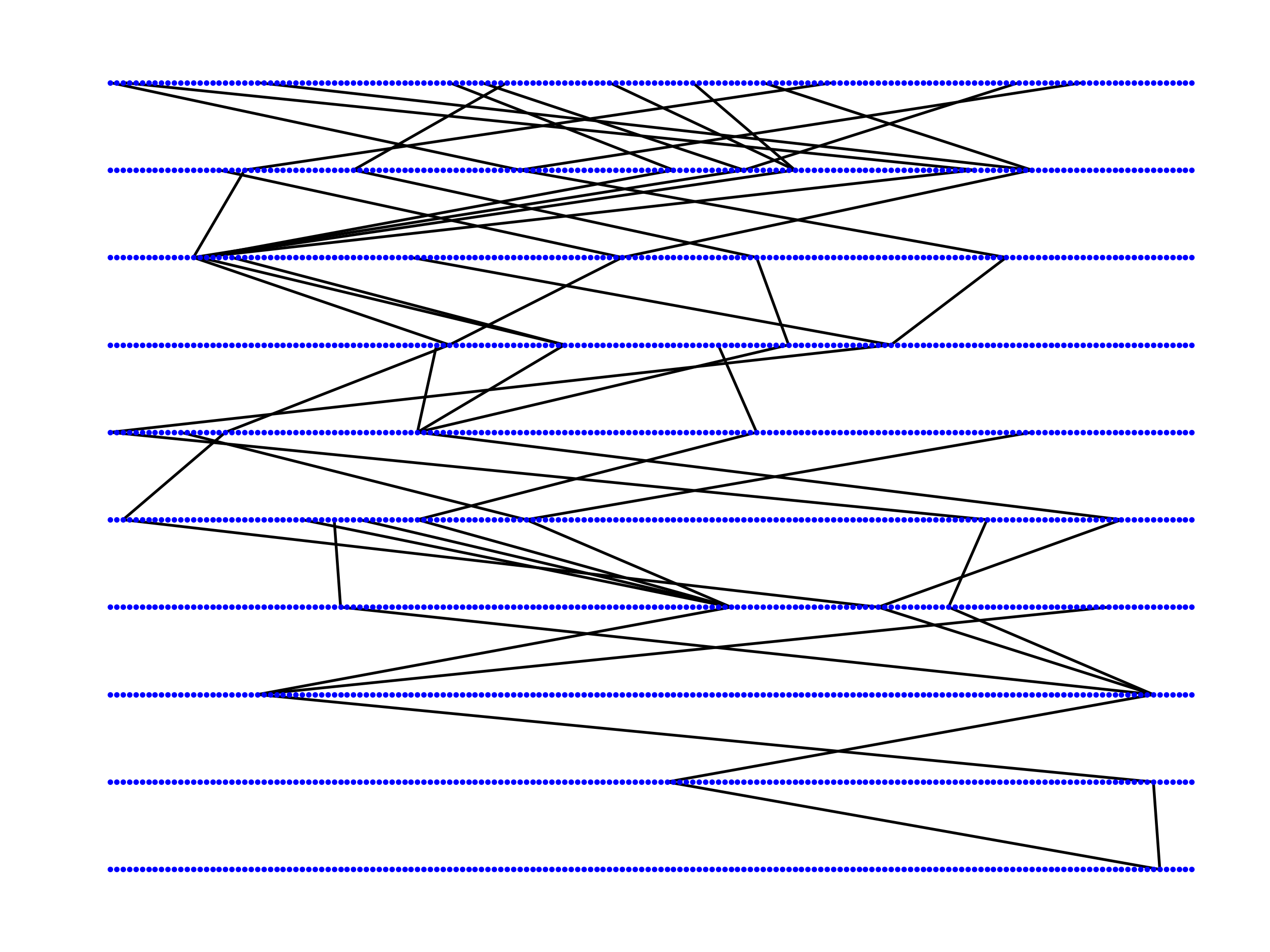
Figure 1. A connected component in a sample of $\mathcal{G}_{\mu}$, for a $\mu$ with heavy, but truncated tails.

For $p\in(0,1)$ define the random $\pm 1$ field $X_{p}:\mathbb{Z}^{2}\to\{+1,-1\}$ by sampling the random graph $\mathcal{G}_{\mu}$ and assigning to each connected component of $\mathcal{G}_{\mu}$ either $+1$ or $-1$ independently with probabilities $p$ and $1-p$ respectively. Precisely, if $(T_{\beta})_{\beta\in I}$ denotes the (random) connected components of $\mathcal{G}_{\mu}$, and $(B_{\beta})_{\beta\in I}$ is a collection of i.i.d. random variables taking the values $+1$ or $-1$, with probabilities $p$ and $1-p$ respectively, then we define $X_{p}(n,t)=\sum_{\beta\in I}1_{T_{\beta}}(n,t)B_{\beta}$. Finally, define the random field $S(n,t)$ by

$$S(n,t)=\sum_{i=1}^{n}X_{p}(i,t).$$

We restrict our attention to the following class of measures, which are the symmetric probability measures in the domain of attraction of a stable law with parameter $\alpha$.

Definition 1.1.

We say that $\mu\in\Gamma_{\alpha}$ if for some slowly varying $L:\mathbb{R}_{+}\to\mathbb{R}_{+}$

1. $\mu(\{-n\})=\mu(\{n\})$,

2. $\mu(\{n,n+1,...\})=L(n)n^{-\alpha}$,

3. the greatest common divisor of $\operatorname{supp}(\mu)$ is $1$,

for all $n\in\mathbb{N}$. Recall that $L:\mathbb{R}_{+}\to\mathbb{R}_{+}$ is slowly varying if for each $c\in(0,\infty)$

$$\lim_{x\to\infty}\frac{L(cx)}{L(x)}=1.$$

Condition $(3)$ is technically convenient, although not necessary. When $\mu\in\Gamma_{\alpha}$, we prove that the random field $S(n,t)$ rescales to a two dimensional Gaussian process $W_{\alpha}$ defined below.

Theorem 1.2.

Let $p,\alpha\in(0,1)$, and $\mu\in\Gamma_{\alpha}$ for some slowly varying function $L:\mathbb{R}_{+}\to\mathbb{R}_{+}$. Define $\sigma_{n}$ by

$$\sigma_{n}^{2}=\tilde{c}_{p}n^{1+\alpha}L(n)^{-1},$$

where $\tilde{c}_{p}$ is the deterministic constant given in Lemma 3.1. Then the random field

$$S_{n}(x,t):\mathbb{R}^{2}\to\mathbb{R}^{2}\ :\ (x,t)\to\frac{1}{\sigma_{n}}\Big{(}S(\lfloor xn\rfloor,\lfloor tn^{\alpha}L(n)^{-1}\rfloor)-(2p-1)\lfloor xn\rfloor\Big{)}$$

converges in distribution to $W_{\alpha}(x,t)$ as $n\to\infty$.

Remark 1.3.

From the proof it is clear that one could replace the independent random variables $(B_{\beta})_{\beta\in I}$ used to construct $S(n,t)$ with any family of independent random variables having 3 bounded moments. In this sense the proof of Theorem 1.2 yields an invariance principle.

The random field $W_{\alpha}(x,t)$ is defined as follows.

Definition 1.4.

Let $W_{\alpha}(x,t)$ be the unique Gaussian random field on $\mathbb{R}^{2}$ with covariance given by

(1.1) $$\operatorname{Cov}(W_{\alpha}(x_{1},t_{1}),W_{\alpha}(x_{2},t_{2}))=\\ \frac{1}{2V(0,1)}\Big{(}V(t_{2}-t_{1},x_{1})|x_{1}|^{1+\alpha}+V(t_{2}-t_{1},x_{2})|x_{2}|^{1+\alpha}-V(t_{2}-t_{1},|x_{2}-x_{1}|)|x_{2}-x_{1}|^{1+\alpha}\Big{)},$$

where $V(t,x)$ is defined as

$$V(t,x)=\int_{0}^{\infty}\frac{1-\cos(u)}{u^{2+\alpha}}e^{-c_{\alpha}\frac{t}{x^{\alpha}}u^{\alpha}}\,du,$$

where $c_{\alpha}=\cos(\frac{\alpha\pi}{2})\Gamma(1-\alpha)$.

It is interesting to consider some aspects of the field $W_{\alpha}$. It is self-similar under the scaling $W_{\alpha}(x,t)\stackrel{{\scriptstyle d}}{{=}}\frac{1}{r^{\frac{1}{2}(1+\alpha)}}W(rx,r^{\alpha}t)$. In particular, for each fixed $t\in\mathbb{R}$, $W_{\alpha}(\cdot,t)$ is fractional Brownian motion with Hurst parameter $1/2+\alpha/2$. In the $t$-direction we see that for each fixed $x\in\mathbb{R}$, $W_{\alpha}(x,\cdot)$ is a stationary Gaussian process. In this sense, $W_{\alpha}$ is a dynamical version of fractional Brownian motion. As $\alpha\to 0$ the family of one dimensional Gaussian processes $(W_{\alpha}(\cdot,t))_{t\in\mathbb{R}}$ behaves like a family of Brownian motions, evolving in time under the Ornstein-Uhlenbeck process. In view of Theorem 1.2, one heuristic for this is to recall the following natural dynamics on the simple random walk. At time $0$ sample a simple random walk with $n$ steps. At time $1$ update the random walk by choosing one of the $n$ steps uniformly at random and independently resampling the $\pm 1$ value there. Repeating this update process gives a family of random walks indexed in time. Rescaling the family of random walks yields a family of Brownian motions evolving according to Ornstein-Uhlenbeck processes. As $\alpha\to 0$ the measure $\mu$ has larger and larger tails so from time $t$ to $t+1$, the $\pm 1$ value at $(n,t+1)$ is effectively being sampled uniformly at random with some probability.

As a corollary of Theorem 1.2 we derive the scaling limit of the voter model with long range interactions. Recall that given $\mu$ on $\mathbb{Z}$, we can define the voter model as the Markov process on $\{-1,+1\}^{\mathbb{Z}}$ whose transition function is the product measure

$$P(\eta,\cdot)=\prod_{i\in\mathbb{Z}}\rho_{i,\eta}(\cdot),$$

where $\rho_{m,\eta}(\xi)=\sum_{n\in\mathbb{Z}}\mu(\{n\})1_{\eta(m-n)=\xi(m)}$ for $\xi:\mathbb{Z}\to\{-1,+1\}$. In other words, given $\eta_{t}$, we can sample $\eta_{t+1}(m)$, by making a independent sample of $\mu$, say $k_{m}$, and adopting the value $\eta_{t}(m-k_{n})$. When $\mu\in\Gamma_{\alpha}$ the Markov process has a one parameter family of extremal invariant measures $\{\nu_{p}\ |p\in[0,1]\}$. See [11] for more background on the voter model.

Theorem 1.5.

Let $p,\alpha\in(0,1)$, $\mu\in\Gamma_{\alpha}$ for some $L:\mathbb{R}_{+}\to\mathbb{R}_{+}$ slowly varying, and $\xi:\mathbb{Z}\to\{+1,-1\}$ be a random function with law $\nu_{p}$. If $F^{n}_{p}:\mathbb{R}\to\mathbb{R}$ is the random field defined on $\phi\in\mathcal{S}(\mathbb{R})$ by

$$F^{n}_{p}(\phi)=\frac{1}{\sigma_{n}\sqrt{\alpha(\alpha/2+1/2)}}\sum_{i\in\mathbb{Z}}\phi\left(\frac{i}{n}\right)(\xi(i)-(2p-1))$$

then $F_{p}^{n}$ converges weakly as a probability measure on tempered distributions to $FGF_{\alpha/2}$, the fractional Gaussian field on $\mathbb{R}$ with index $\frac{\alpha}{2}$. Here $\sigma_{n}$ is as given in Theorem 1.2.

The fractional Gaussian field on $\mathbb{R}^{d}$ with index $h$, denoted $FGF_{h}(\mathbb{R}^{d})$, can be defined as a random tempered distribution given by $(-\Delta)^{-h/2}W$, where $W$ is Gaussian white noise on $\mathbb{R}^{d}$. $FGF_{\alpha/2}$ is known as fractional Gaussian noise and given a test function $\phi$, $FGF_{\alpha/2}(\phi)$ is a Gaussian random variable with variance

$$\int_{\mathbb{R}}\int_{\mathbb{R}}\frac{\phi(x)\phi(y)}{|x-y|^{1-\alpha}}dxdy.$$

For comparison, when $\mu$ is sufficiently short range on $\mathbb{Z}^{3}$, the voter model also has a one parameter family of invariant measures, and Bramson-Griffeath [3] proved in that case the voter model rescales to $FGF_{1}(\mathbb{R}^{3})$, the Gaussian free field. For more on fractional Gaussian fields see the survey [14].

1.3. A Brief Proof Sketch

The first step to Theorem 1.2 is to ensure that the random graph $\mathcal{G}_{\mu}$ has infinitely many connected components when $\alpha\in(0,1)$. It is natural to expect that this happens for $\alpha\in(0,1)$ since a random walk with step distribution $\mu$ is recurrent whenever $\alpha>1$ and transient whenever $\alpha<1$. The next step is to derive the asymptotic covariance of the field $S(n,t)$. This is done with a Fourier analytic argument, using an idea from [10]. We note that the techniques in [10] need to be revised since the multi-dimensional nature of the model does not allow one to directly apply a Tauberian theorem.

To finish the proof of Theorem 1.2 we need to prove $S(n,t)$ is asymptotically Gaussian. As opposed to prior works which use a martingale central limit theorem, we take a component based approach using the Lindeberg exchange method. If $(T_{\beta})_{\beta\in I}$ are the connected components of $\mathcal{G}_{\mu}$, then $S(n,0)=\sum_{i=1}^{n}X_{i,t}=\sum_{\beta}B_{\beta}|T_{\beta}\cap[0,n]\times\{0\}|$. So $S(n,0)$ is a sum of independent Bernoulli random variables with random weights coming from the sizes of the connected components in $[0,n]\times\{0\}$. If all the $|T_{\beta}\cap[0,n]\times\{0\}|$ were deterministic and asymptotically made small contributions, one could apply the standard Lindeberg swapping method to conclude the sum is nearly Gaussian. While the $|T_{\beta}\cap[0,n]\times\{0\}|$ are not deterministic, they are independent of the random variables $(B_{\beta})_{\beta\in I}$ and one can show that with high probability no single connected component “dominates” the sum. This is enough to adapt the Lindeberg swapping method. The main technical points here are moment and covariance bounds on $|T_{\beta}\cap[0,n]\times\{t\}|$ proved in section $5$.

Once Theorem 1.2 is proven, Theorem 1.5 is a straightforward corollary, and the main thing to check is that restricted to a time slice, $X_{p}$ has the law of $\nu_{p}$. This is done in Section 6.

1.4. Notation

Throughout the paper $C>1>c>0$ denote constants that may differ in each instance and depend on $\mu$. Any further dependencies will be explicitly stated.

1.5. Acknowledgements

The author is grateful to Alan Hammond for suggesting this problem and stimulating discussions. The author would also like to thank Charles Smart for useful discussions and encouragement, and Adam Black for helpful comments on an earlier draft of the paper.

2. Number of Components of $\mathcal{G}_{\mu}$

Our first result relates the rate of tail decay of $\mu$ to the number of connected components of $\mathcal{G}_{\mu}$. We refer to $(n-J_{(n,t)},t-1)$ as the parent of $(n,t)$, and use the term ancestral line of $(n,t)$ to refer to the unique sequence of vertices starting at $(n,t)$ for which the next vertex in the sequence is the parent of the current vertex. Note the law of the ancestral line of $(n,t)$ is given by a random walk started at $(n,t)$ with jump distribution $\mu$. We write $(n_{1},t_{1})\sim(n_{2},t_{2})$ if the ancestral lines of $(n_{1},t_{1})$ and $(n_{2},t_{2})$ merge at some point.

Proposition 2.1.

Suppose $\mu\in\Gamma_{\alpha}$. If $\alpha>1$ then $\mathcal{G}_{\mu}$ has one connected component almost surely, and if $\alpha<1$ then $\mathcal{G}_{\mu}$ has infinitely many connected components almost surely.

Proof.

Sample two independent ancestral lines $A_{(0,0)}$ and $\tilde{A}_{(0,0)}$ both started at $(0,0)$.

Claim 1: If $\mathbb{E}|A_{(0,0)}\cap\tilde{A}_{(0,0)}|=\infty$ then $\mathcal{G}_{\mu}$ has one connected component almost surely and if $\mathbb{E}|A_{(0,0)}\cap\tilde{A}_{(0,0)}|<\infty$, then $\mathcal{G}_{\mu}$ has infinitely many connected components almost surely.

Since the greatest common divisor of the support of $\mu$ is $1$, we have that $\mathbb{E}|A_{(0,0)}\cap\tilde{A}_{(0,0)}|=\infty$ implies $\mathbb{P}((n,0)\sim(0,0))=1$ for each $n\in\mathbb{Z}$. So $\mathcal{G}_{\mu}$ has 1 connected component almost surely. On the other hand if $\mathbb{E}|A_{(0,0)}\cap\tilde{A}_{(0,0)}|<\infty$ then we argue that $\mathbb{P}((k,0)\sim(0,0))\to 0$ as $k\to\infty$. To see this let $q_{n,t}:=\mathbb{P}((n,t)\in A_{(0,0)})$ and note that

$$\mathbb{E}|A_{(0,0)}\cap\tilde{A}_{(0,0)}|=1+\sum_{n\in\mathbb{Z},t<0}q_{n,t}^{2}<\infty.$$

In particular this implies that if $A_{(k,0)}$ is an ancestral line started at $(k,0)$ and independent of $A_{(0,0)}$

$$\mathbb{E}|A_{(0,0)}\cap A_{(k,0)}|\to 0$$

as $k\to\infty$, since

$$\mathbb{E}|A_{(0,0)}\cap A_{(k,0)}|=\sum_{n\in\mathbb{Z},t<0}q_{n-k,t}q_{n,t}\to 0\ as\ k\to\infty.$$

By the relation $\mathbb{E}|A_{(k,0)}\cap A_{(0,0)}|=\mathbb{P}((k,0)\sim(0,0))\mathbb{E}|A_{(0,0)}\cap\tilde{A}_{(0,0)}|$, we see that $\mathbb{P}((k,0)\sim(0,0))\to 0$ as $k\to\infty$. Now the infinitude of the components follows from Borel-Cantelli. Indeed, choose a sequence $a_{0}<a_{1}<...\to\infty$, and define the events

$$E_{l}=\{(a_{l},0)\not\sim(a_{j},0)\ \forall 0\leq j<l\}.$$

Since $\mathbb{P}((k,0)\sim(0,0))\to 0$ as $k\to\infty$ we may take the sequence $(a_{n})$ to infinity fast enough that $\mathbb{P}(E_{l}^{c})\leq\sum_{k=0}^{l}\mathbb{P}((a_{l},0)\sim(a_{k},0))\leq\frac{10}{l^{2}}$. By Borel-Cantelli infinitely many $E_{j}$ happen almost surely and hence $\mathcal{G}_{\mu}$ has infinitely many connected components almost surely.

Claim 2: $\mathbb{E}|A_{(0,0)}\cap\tilde{A}_{(0,0)}|=\infty$ if $\alpha>1$ and $\mathbb{E}|A_{(0,0)}\cap\tilde{A}_{(0,0)}|<\infty$ if $\alpha<1$.

Let $p_{n}:=\mu(\{n\})$ and define

$$P(x)=\sum e^{inx}p_{n},$$

and

$$Q(x,y)=\frac{1}{1-e^{-iy}P(x)}.$$

Note that $\widehat{Q}(n,t)=q_{n,t}=\mathbb{P}((n,t)\in A_{(0,0)})$, and thus

$$\mathbb{E}|A_{(0,0)}\cap\tilde{A}_{(0,0)}|=||Q||^{2}_{L^{2}(\mathbb{T}^{2})}.$$

Since $\mu\in\Gamma_{\alpha}$ we have by Theorem 1 in [9]

(2.1) $$|1-P(x)|=c_{\alpha}x^{\alpha}L(x^{-1})+o(x^{\alpha}L(x^{-1}))$$

as $x\to 0$, where

$$c_{\alpha}=\cos\left(\frac{\alpha\pi}{2}\right)\Gamma(1-\alpha).$$

Calculating we see that $\int_{\mathbb{T}^{2}}\frac{1}{|1-e^{-iy}P(x)|^{2}}\,dx\,dy=\infty$ if $\alpha>1$, and is finite if $\alpha<1$. ∎

We note that when $\alpha=1$, the number of connected components of $\mathcal{G}_{\mu}$ can depend on the slowly varying function $L(x)$.

3. Asymptotics for the Variance

For the remainder of the paper we assume $\mu\in\Gamma_{\alpha}$. Let $p\in(0,1)$ and let $S(n,t)=\sum_{m=0}^{n}X_{p}(m,t),$ where $X_{p}$ is as defined in section 1.2.

Lemma 3.1.

For any $p\in(0,1)$ and $t,x_{1},x_{2}\in\mathbb{R}$ we have

(3.1) $$\operatorname{Cov}\Big{(}S(\lfloor x_{1}n\rfloor,0),\ S(\lfloor x_{2}n\rfloor,\lfloor tL(n)^{-1}n^{\alpha}\rfloor)\Big{)}\\ =\tilde{c}_{p}n^{1+\alpha}L(n)^{-1}\Big{(}V(t,x_{1})|x_{1}|^{1+\alpha}+V(t,x_{2})|x_{2}|^{1+\alpha}+V(t,|x_{2}-x_{1}|)|x_{1}-x_{2}|^{1+\alpha}\Big{)}\\ +o(n^{1+\alpha}L(n)^{-1})$$

as $n\to\infty$, where

$$V(t,x)=\int_{0}^{\infty}\frac{1-\cos(u)}{u^{2+\alpha}}e^{-c_{\alpha}\frac{t}{x^{\alpha}}u^{\alpha}}\,du$$

and

$$\tilde{c}_{p}=\frac{2p(1-p)}{\pi c_{\alpha}||Q||_{L^{2}}^{2}}.$$

Remark 3.2.

It may surprising at first glance that $t\sim n^{\alpha}$ is the correct time-scale for $S(n,t)-S(n,0)$ to exhibit sizable fluctuations. Indeed, one is re-sampling all values at each time step. A heuristic explanation for this timescale is that a random walk with step distribution $\mu$ will take $\sim n^{\alpha}$ steps to leave a neighborhood of size $n$. So roughly $n^{\alpha}$ time steps are needed for a macroscopic proportion of the current values between $(0,0)$ and $(n,0)$ to “exit” the interval between $(0,0)$ and $(n,0)$ and be replaced by new values. Lemmas 4.1 and 4.2 make this heuristic more precise.

Proof.

It suffices to consider $x_{1},x_{2},t\in\mathbb{R}_{\geq 0}$. Let $n_{1}=\lfloor x_{1}n\rfloor,\ n_{2}=\lfloor x_{2}n\rfloor$, $t_{1}=\lfloor tL(n)^{-1}n^{\alpha}\rfloor$ and compute

$$\operatorname{Cov}\Big{(}S(n_{1},0),\ S(n_{2},t_{1})\Big{)} =\sum_{0\leq k_{2}\leq n_{2}}\sum_{0\leq k_{1}\leq n_{1}}\operatorname{Cov}(X_{k_{1},0},\ X_{k_{2},t_{1}})$$

$$=4p(1-p)\sum_{0\leq k_{2}\leq n_{2}}\sum_{0\leq k_{1}\leq n_{1}}\mathbb{P}((k_{1}-k_{2},t_{1})\sim(0,0)).$$

Counting the number of pairs $(k_{1},k_{2})\in[0,n_{1}]\times[0,n_{2}]$ such that $|k_{1}-k_{2}|=k$ we see that

(3.2) $$\operatorname{Cov}\Big{(}S(n_{1},0),\ S(n_{2},t_{1})\Big{)}=4p(1-p)\Bigg{(}\sum_{k=0}^{n_{1}}(n_{1}-k)\mathbb{P}((k,t_{1})\sim(0,0))+\sum_{k=0}^{n_{2}}(n_{2}-k)\mathbb{P}((k,t_{1})\sim(0,0))\\ -\sum_{k=0}^{|n_{2}-n_{1}|}(|n_{2}-n_{1}|-k)\mathbb{P}((k,t_{1})\sim(0,0))\Bigg{)}+O(n).$$

It suffices to work out the asymptotics for $\sum_{k=0}^{n_{1}}(n_{1}-k)\mathbb{P}((k,t_{1})\sim(0,0))$ since the other sums are of the same form. The key observation is that if $\tilde{A}_{(0,0)}$, $A_{(0,0)}$, and $A_{(k,t)}$ are all independent ancestral lines started at $(0,0),\ (0,0),\$ and $(k,t)$, respectively, then

$$\frac{\mathbb{E}|A_{(0,0)}\cap A_{(k,t)}|}{\mathbb{E}|A_{(0,0)}\cap\tilde{A}_{(0,0)}|}=\mathbb{P}((0,0)\sim(k,t)).$$

Recalling the characteristic function of $\mu$,

$$P(x)=\sum_{n\in\mathbb{Z}}\mu(\{n\})e^{inx},$$

we see

$$\mathbb{E}|A_{(0,0)}\cap A_{(k,t)}|=\sum_{s=0}^{\infty}\widehat{P^{t+2s}}(k)=\widehat{\frac{P^{t}}{1-P^{2}}}(k).$$

Now compute for $t_{1}\geq 0$

$$\sum_{k=0}^{n_{1}}(n_{1}-k)\mathbb{P}((k,t_{1})\sim(0,0)) =\frac{1}{\mathbb{E}|A_{(0,0)}\cap\tilde{A}_{(0,0)}|}\sum_{k=0}^{n_{1}}(n_{1}-k)\mathbb{E}|A_{(0,0)}\cap A_{(k,t_{1})}|$$

$$=\frac{1}{||Q||^{2}_{L^{2}}}\sum_{k=0}^{n_{1}}(n_{1}-k)\widehat{\frac{P^{t_{1}}}{1-P^{2}}}(k)$$

$$=\frac{1}{2\pi||Q||^{2}_{L^{2}}}\int_{0}^{2\pi}\left(\sum_{k=0}^{n_{1}}(n_{1}-k)\cos(kx)\right)\frac{P^{t_{1}}(x)}{1-P^{2}(x)}dx$$

The sum inside the integral is $\frac{n_{1}}{2}F_{n_{1}}(x)+\frac{n_{1}}{2}$, where $F_{N}(x)=\sum_{|k|\leq N}\big{(}1-\frac{|k|}{N}\big{)}e^{ikx}=\frac{1}{N}\big{(}\frac{1-\cos(nx)}{1-\cos(x)}\big{)}$ is the Fejér kernel. Thus

(3.3) $$\begin{split}\sum_{k=0}^{n_{1}}(n_{1}-k)\mathbb{P}((k,t_{1})\sim(0,0))&=\frac{n_{1}}{2\pi||Q||^{2}_{L^{2}}}\int_{0}^{\pi}\frac{1-\cos(n_{1}x)}{n_{1}(1-\cos(x))}\frac{P^{t_{1}}(x)}{1-P^{2}(x)}dx+O(n_{1})\\ &=\frac{n_{1}^{1+\alpha}L(n_{1})^{-1}}{2\pi||Q||_{2}^{2}}\int_{0}^{\pi n_{1}}\frac{1-\cos(u)}{n_{1}^{2}\big{(}1-\cos\big{(}\frac{u}{n_{1}}\big{)}\big{)}}P^{t_{1}}\Big{(}\frac{u}{n_{1}}\Big{)}\frac{L(n_{1})}{n_{1}^{\alpha}\big{(}1-P^{2}\big{(}\frac{u}{n_{1}}\big{)}\big{)}}du+O(n_{1})\\ &:=\frac{n_{1}^{1+\alpha}L(n_{1})^{-1}}{2\pi||Q||_{2}^{2}}\int_{0}^{\pi n_{1}}A_{n}(u)B_{n}(u)C_{n}(u)+O(n_{1}),\end{split}$$

where we used that the integrand was even to integrate from $0$ to $\pi$ and made the change of variables $u=n_{1}x$ in the second step. Recall that $(n_{1},t_{1})=(\lfloor x_{1}n\rfloor,\lfloor tL(n)^{-1}n^{\alpha}\rfloor)$.

To compute the asymptotics in $n$ we claim we may apply dominated convergence. The standard bound on the Fejér kernel implies $|F_{N}(x)|\leq C\min(N,\frac{1}{Nx^{2}})$ (see [15] chapter 1) and by definition $|P(x)|\leq 1$ so that $|B_{n}(u)A_{n}(u)|\leq\frac{C}{1+u^{2}}$. Further by (2.1) and Potters Theorem for slowly varying functions (Theorem 1.5.6 in [2]) applied to $C_{n}(u)$ we obtain

$$|A_{n}(u)B_{n}(u)C_{n}(u)|\leq\Big{(}\frac{C}{u^{\alpha}(1+u^{2})}\Big{)}\frac{L(n_{1})}{L(\frac{n_{1}}{u})}\leq\frac{C(u^{\epsilon}+u^{-\epsilon})}{u^{\alpha}(1+u^{2})}$$

for any $\epsilon>0$ where $C$ may depend on $\epsilon$, $x_{1}$ and $t$. The above function is clearly integrable for $\epsilon$ small, so it suffices to compute the pointwise limits of $A_{n}(u),B_{n}(u),$ and $C_{n}(u)$. Fix $u\in\mathbb{R}$ and estimate

$$A_{n}(u)=\frac{1-\cos(u)}{n_{1}^{2}\big{(}1-\cos\big{(}\frac{u}{n_{1}}\big{)}\big{)}}=\frac{2(1-\cos(u))}{u^{2}}+O(n_{1}^{-2}).$$

For $B_{n}$ we use the asymptotics (2.1) and the fact that $(1-x)^{x}\to e^{-1}$ as $x\to 0$ to estimate

$$B_{n}(u) =\Big{(}1-\Big{(}1-P\Big{(}\frac{u}{n_{1}}\Big{)}\Big{)}^{t_{1}}$$

$$=e^{-c_{\alpha}\frac{t}{x^{\alpha}}u^{\alpha}}+o(1),$$

where $c_{\alpha}$ is as used in (2.1). Lastly, for $C_{n}$ we again use the asymptotics (2.1) to get

$$C_{n}(u) =\frac{L(n_{1})}{n_{1}^{\alpha}(1-P^{2}(\frac{u}{n_{1}}))}$$

$$=\Big{(}\frac{1}{1+P(\frac{u}{n_{1}})}\Big{)}\frac{L(n_{1})}{n_{1}^{\alpha}\big{(}1-P\big{(}\frac{u}{n_{1}}\big{)}\big{)}}$$

$$=\frac{1}{2c_{\alpha}u^{\alpha}}+o(1)$$

Plugging this into (3.3) gives

$$\sum_{k=0}^{n_{1}}(n_{1}-k)\mathbb{P}((k,t_{1})\sim(0,0))=\frac{n_{1}^{1+\alpha}L(n_{1})^{-1}}{2c_{\alpha}\pi||Q||_{2}^{2}}\int_{0}^{\infty}\frac{1-\cos(u)}{u^{2+\alpha}}e^{-\frac{c_{\alpha}t}{x^{\alpha}}u^{\alpha}}du+O(n_{1}).$$

Computing the asymptotics of the other terms in (3.2) and recalling that $L(x)$ is slowly varying yields the claim. ∎

4. Estimates on the Random Graph $\mathcal{G}_{\mu}$

To apply a Lindeberg swapping type argument the main technical obstacle is to ensure that the connected components are roughly the same size. This is achieved by the second moment and covariance estimates in this section, which rest on the heat kernel bounds proved below.

4.1. A Heat Kernel Estimate

We will need the following estimate for random walks with jump kernel $\mu$. It quantifies the rate of transience of the random walk generated by $\mu$.

Lemma 4.1.

Let $p_{t}(x,y)$ be the $t$-step transition kernel of the random walk on $\mathbb{Z}$ generated by $\mu$ and started at $x$. Then for each $\epsilon>0$, there exists $C>0$ depending on $\epsilon$, such that

(4.1) $$||p_{t}(x,y)||_{\infty}\leq Ct^{-1/(\alpha+\epsilon)}.$$

The above lemma essentially follows from the local limit law. Our proof adapts the proof of the local limit law for stable laws given in [8]. To put the above bound in context we recall that if $\mu$ satisfies the pointwise bounds

$$\frac{\kappa^{-1}}{(1+|n|)^{1+\alpha}}\leq p_{n}=\mu(\{n\})\leq\frac{\kappa}{(1+|n|)^{1+\alpha}},$$

then it is known (see [1] for instance) that

(4.2) $$c_{2}\min\left(t^{-1/\alpha},\frac{n}{|n|^{1+\alpha}}\right)\leq p_{t}(0,n)=q_{(n,-t)}\leq c_{1}\min\left(t^{-1/\alpha},\frac{n}{|n|^{1+\alpha}}\right).$$

Proof.

Fix $\epsilon>0$ sufficiently small, and recall the characteristic function of $\mu$

$$P(x)=\hat{\mu}(x)=\sum_{m\in\mathbb{Z}}e^{imx}\mu(m).$$

Since $\mu$ is regularly varying with $\operatorname{supp}(\mu)$ having greatest common divisor $1$, we have the estimate

(4.3) $$|P(x)|\leq 1-c|x|^{\alpha+\epsilon}$$

for each $x\in[-\pi,\pi]$, where $c$ may depend on $\epsilon$ and $\mu$. Writing $p_{t}(0,\cdot)$ in terms of $P$ by Fourier inversion and using the above bound gives

$$|p_{t}(0,n)|=|\frac{1}{2\pi}\int_{0}^{2\pi}e^{-inx}P^{t}(x)\,dx| \leq\frac{1}{2\pi}\int_{|x|\leq t^{-1/(\alpha+\epsilon)}}(1-c|x|^{\alpha+\epsilon})^{t}\,dx$$

$$\qquad\qquad\qquad\qquad+\frac{1}{2\pi}\int_{t^{-1/(\alpha+\epsilon)}<|x|\leq\pi}(1-c|x|^{\alpha+\epsilon})^{t}\,dx$$

$$\leq Ct^{-1/(\alpha+\epsilon)}+C\int_{t^{-1/(\alpha+\epsilon)}<|x|\leq\pi}(1-c|x|^{\alpha+\epsilon})^{t}\,dx.$$

To show the second integral is $\leq Ct^{-1(\alpha+\epsilon)}$, we make the change of variables $x=yt^{-1/(\alpha+\epsilon)}$ and compute

$$\int_{t^{-1/(\alpha+\epsilon)}<|x|\leq\pi}(1-|x|^{\alpha+\epsilon})^{t}\,dx =2t^{-1/(\alpha+\epsilon)}\int_{1}^{t^{-1/(\alpha+\epsilon)}\pi}\Big{(}1-c\frac{y^{\alpha+\epsilon}}{t}\Big{)}^{t}\,dy$$

$$\leq Ct^{-1/(\alpha+\epsilon)}\int_{1}^{\infty}e^{-cy^{\alpha+\epsilon}}\,dy$$

$$\leq Ct^{-1/(\alpha+\epsilon)}.$$

∎

Using the Lemma 4.1 we prove the following estimate for the total amount of time the random walk started at $k\in\mathbb{Z}$ and generated by $\mu$ spends in any interval of length $n$.

Lemma 4.2.

Fix $\epsilon>0$. Then there exists $C>0$, depending on $\epsilon$, such that for any $k\in\mathbb{Z}$ and $n\in\mathbb{Z}_{>0}$ we have

(4.4) $$\sum_{0\leq n_{1}\leq n}\sum_{t\geq 0}p_{t}(0,n_{1}-k)\leq Cn^{\alpha+\epsilon}.$$

Proof.

Without loss of generality we may take $0<\epsilon<1-\alpha$. By Lemma 4.1 we have for each $t\geq 1$

$$\sum_{0\leq n_{1}\leq n}p_{t}(0,n_{1}-k)\leq Cnt^{-1/(\epsilon+\alpha)}$$

We also have the bound

$$\sum_{0\leq n_{1}\leq n}p_{t}(0,n_{1}-k)\leq 1,$$

for all $t\geq 0$. Using both we estimate, using that $\epsilon<1-\alpha$

$$\sum_{t\geq 0}\sum_{0\leq n_{1}\leq n}p_{t}(0,n_{1}-k) \leq\sum_{0\leq t\leq n^{\alpha+\epsilon}}\sum_{0\leq n_{1}\leq n}p_{t}(0,n_{1}-k)+\sum_{n^{\alpha+\epsilon}\leq t}\sum_{0\leq n_{1}\leq n}p_{t}(0,n_{1}-k)$$

$$\leq n^{\alpha+\epsilon}+Cn\sum_{n^{\alpha+\epsilon}\leq t}t^{-1/(\alpha+\epsilon)}$$

$$\leq Cn^{\alpha+\epsilon}$$

∎

4.2. Moment Bounds on Connected Components

For any $S\subset\mathbb{Z}^{2}$ and $q\in\mathbb{Z}^{2}$ let $T_{q}^{S}=\{q_{0}\in S|q\sim q_{0}\}$. $T_{q}^{S}$ is the set of points in $S$ which are in the same connected component of $\mathcal{G}_{\mu}$ as $q$. In this section we establish the following two estimates.

Lemma 4.3.

Fix $\epsilon>0$ and $S=[0,n]\times\{0\}$. Then there exists $C>0$, depending on $\epsilon$, such that for each $q\in S$ and $n\in\mathbb{Z}_{>0}$

(4.5) $$\mathbb{E}|T_{q}^{S}|^{2}\leq Cn^{2\alpha+\epsilon}.$$

Lemma 4.4.

Fix $\epsilon>0$, and $S=\cup_{j=1}^{k}[0,x_{k}n]\times\{t_{k}\}$. Then there exists $C>0$, depending on $x_{i}$, $t_{i}$, and $\epsilon$, such that for each $q\in S$ and $n\in\mathbb{Z}_{>0}$

(4.6) $$\sum_{q_{0}\in S}\operatorname{Cov}\Big{(}|T_{q}^{S}|,|T_{q_{0}}^{S}|\Big{)}\leq Cn^{3\alpha+\epsilon}.$$

For comparison if $S=[0,n]\times\{0\}$, our variance estimates show that $\mathbb{E}|T_{(0,0)}^{S}|=O(L(n)n^{\alpha})$. So, Lemma 4.3 tells us that $|T_{(0,0)}^{S}|$ is $O(n^{\alpha+\epsilon})$ with high probability. Lemma 4.4 says that in a weak sense $|T_{(0,0)}^{S}|$ and $|T_{(m,0)}^{S}|$ behave independently when $(m,0)\notin T_{(0,0)}^{S}$.

Proof of Lemma 4.3.

Without loss of generality we can assume $q=(0,0)$. First we estimate the number of points in $[0,n]\times\{0\}$ who’s ancestral lines merge with that of a given point. In what follows we use the shorthand $p_{t}(n):=p_{t}(0,n)=p_{t}(k,k+n)$, and define $p_{t}(k)=0$ for all $t<0$. For any $(j,s)\in\mathbb{Z}^{2}$ we have

(4.7) $$\sum_{0\leq n_{1}\leq n}\mathbb{P}((n_{1},0)\sim(j,s)) =\sum_{0\leq n_{1}\leq n}\frac{\mathbb{E}|A_{(n_{1},0)}\cap A_{(j,s)}|}{\mathbb{E}|A_{(0,0)}\cap\tilde{A}_{(0,0)}|}$$

$$\leq C\sum_{0\leq n_{1}\leq n}\sum_{(k,t)\in\mathbb{Z}^{2}}p_{t}(k-n_{1})p_{t+s}(j-k)$$

$$\leq C\sum_{0\leq n_{1}\leq n}\sum_{t\geq 0}p_{2t+s}(j-n_{1})$$

$$\leq Cn^{\alpha+\epsilon},$$

where we used the semi-group property of $p_{t}(x,y)$ summing over $k$ in the second inequality, and then used Lemma 4.2 to finish. To prove 4.3 we compute

$$\mathbb{E}|T_{0}^{S}|^{2}=\mathbb{E}\sum_{0\leq n_{1},n_{2}\leq n}1_{(0,0)\sim(n_{1},0)}1_{(0,0)\sim(n_{2},0)}=\sum_{0\leq n_{1},n_{2}\leq n}\mathbb{P}((0,0)\sim(n_{1},0)\sim(n_{2},0)).$$

The last probability can be bounded as

(4.8) $$\mathbb{P}((0,0)\sim(n_{1},0)\sim(n_{2},0))\leq C\Big{(}\sum_{(k,t)\in\mathbb{Z}^{2}}p_{t}(k)p_{t}(n_{1}-k)\mathbb{P}((k,t)\sim(n_{2},0))\\ +p_{t}(k)p_{t}(n_{2}-k)\mathbb{P}((k,t)\sim(n_{1},0))+p_{t}(n_{2}-k)p_{t}(n_{1}-k)\mathbb{P}((k,t)\sim(0,0))\Big{)}.$$

The first term is the probability that $A_{(0,0)}$ and $A_{(n_{1},0)}$ meet at the point $(k,t)$ and $(n_{2},0)$ is in the same connected component as $(k,t)$. The second and third terms are the same but for the cases that $(0,0)$ and $(n_{2},0)$ meet first or $(n_{2},0)$ and $(n_{1},0)$ meet first respectively. Consider the first term above. Summing it over $n_{1}$ and $n_{2}$ gives

$$\sum_{0\leq n_{1},n_{2}\leq n}\sum_{(k,t)\in\mathbb{Z}^{2}} p_{t}(k)p_{t}(n_{1}-k)\mathbb{P}((k,t)\sim(n_{2},0))$$

$$\leq C\sum_{0\leq n_{1}\leq n}\sum_{(k,t)\in\mathbb{Z}^{2}}p_{t}(k)p_{t}(n_{1}-k)\Big{(}\sum_{0\leq n_{2}\leq n}\mathbb{P}((k,t)\sim(n_{2},0))\Big{)}$$

$$\leq Cn^{\alpha+\epsilon}\sum_{0\leq n_{1}\leq n}\sum_{(k,t)\in\mathbb{Z}^{2}}p_{t}(k)p_{t}(n_{1}-k)$$

$$\leq Cn^{\alpha+\epsilon}\sum_{0\leq n_{1}\leq n}\sum_{t\geq 0}p_{t}(n_{1})$$

$$\leq Cn^{2\alpha+2\epsilon}.$$

From the second to third line we summed over $n_{2}$ and used 4.7, and for the last inequality we used the semigroup property and 4.7 again. Since $\mu$ is symmetric and we are summing over $n_{1},n_{2}\in[0,n]$ the other two terms in 4.8 satisfy the same bound. Thus $\mathbb{E}|T_{0}^{S}|^{2}\leq Cn^{2\alpha+2\epsilon}$. ∎

Next we establish a covariance estimate on the connected components. The coupling arguement used was adapted from Lemma 7.1 in [12].

Proof of Lemma 4.4.

We assume without loss of generality that $q=(0,0)$ and we write $0$ for the point $(0,0)$. To begin compute

(4.9) $$\begin{split}\operatorname{Cov}(|T_{0}^{S}|,|T_{q_{0}}^{S}|)&=\sum_{q_{1},q_{2}\in S}\operatorname{Cov}(1_{0\sim q_{1}},1_{q_{0}\sim q_{2}})\\ &=\sum_{q_{1},q_{2}\in S}\Big{(}\mathbb{P}(0\sim q_{1}\cap q_{0}\sim q_{2})-\mathbb{P}(0\sim q_{1})\mathbb{P}(q_{0}\sim q_{2})\Big{)}.\end{split}$$

We claim each term on the last line above is upper bounded by the probability all 4 points coalesce.

Claim 4.5.

For any $q_{0},q_{1},q_{2}\in\mathbb{Z}^{2}$

(4.10) $$\mathbb{P}(0\sim q_{1}\cap q_{0}\sim q_{2})-\mathbb{P}(0\sim q_{1})\mathbb{P}(q_{0}\sim q_{2})\leq\mathbb{P}(0\sim q_{1}\sim q_{0}\sim q_{2}).$$

We use a coupling argument. Sample independent ancestral lines $A_{0},A_{q_{0}},A_{q_{1}},A_{q_{2}}$ which start at $0,q_{0},q_{1},q_{2}$, and build a random graph $G$ inductively as follows. Start with $G=A_{0}$. If $A_{q_{0}}\cap G\neq\emptyset$ then add to $G$ all points in $A_{q_{0}}$ before the intersection with $G$, otherwise add to $G$ all of $A_{q_{0}}$. Repeat this process with the updated $G$ for $A_{q_{1}}$ and $A_{q_{2}}$. Note that the random graph $G$ is a sample of the random graph $\mathcal{G}_{\mu}$ restricted to the ancestral lines of $0,q_{0},q_{1},q_{2}$ and we can estimate

$$\mathbb{P}(0\sim_{G}q_{1}\not\sim_{G}q_{0}\sim_{G}q_{2}) \leq\mathbb{P}(\{A_{0}\cap A_{q_{1}}\neq\emptyset\}\cap\{A_{q_{0}}\cap A_{q_{2}}\neq\emptyset\})$$

$$=\mathbb{P}(\{A_{0}\cap A_{q_{1}}\neq\emptyset\})\mathbb{P}(\{A_{q_{0}}\cap A_{q_{2}}\neq\emptyset\})$$

$$=\mathbb{P}(0\sim q_{1})\mathbb{P}(q_{0}\sim q_{2}),$$

where $x\sim_{G}y$ means that $x$ and $y$ are in the same connected component of $G$. (4.10) now follows since

$$\mathbb{P}(0\sim q_{1}\cap q_{0}\sim q_{2})=\mathbb{P}(0\sim q_{1}\sim q_{0}\sim q_{2})+\mathbb{P}(0\sim q_{1}\not\sim q_{0}\sim q_{2}).$$

By (4.10) it now suffices to prove

(4.11) $$\sum_{q_{0},q_{1},q_{2}\in S}\mathbb{P}(0\sim q_{0}\sim q_{1}\sim q_{2})\leq Cn^{3\alpha+\epsilon}.$$

We can now handle the sum in the same way as the previous lemma. For clarity we give the argument when $k=1$ and $S=[0,n]\times\{0\}$. Note that we only use the semi-group property and the bound (4.7), hence the same argument works for $S=\cup_{j=1}^{k}[0,x_{j}n]\times\{t_{j}\}$ with straightforward adjustments.

To estimate (4.11) we break the event that $(0,0)\sim(i,0)\sim(k,0)\sim(j,0)$ into cases and estimate each case similarly as done in Lemma 4.3. There are 18 cases since there are $6$ ways to choose which pair of ancestral lines meet first, and then $3$ ways to choose which two ancestral lines coalesce next. Note that these cases are not disjoint, since more than two ancestral lines may merge at a given point. However, up to permuting the vertices, there are only 2 distinct types of sums corresponding to the two different “shapes of coalescence” the ancestral lines can make. Figure 2 depicts the two possible shapes of coalescence. It suffices to estimate the contributions from those two types.

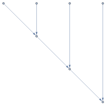
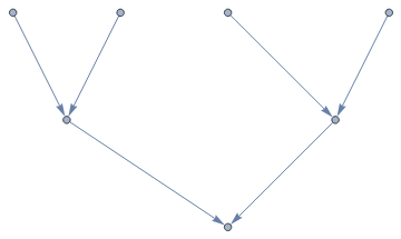
Figure 2. On the left the ancestral lines coalesce one at a time, and on the right the lines coalesce pairwise

The first type, depicted on the left in figure 2, is when the lines coalesce one at a time. Without loss of generality we estimate this by the probability that the ancestral line of $(0,0)$ merges with the ancestral line of $(i,0)$ at $(a_{1},t_{1})$, then merges with the ancestral line of $(j,0)$ at $(a_{2},t_{2})$ (with $t_{2}\leq t_{1}$), and finally with that of $(k,0)$. We can upper bound this by

$$C\sum_{(a_{1},t_{1}),(a_{2},t_{2})\in\mathbb{Z}^{2}}p_{t_{1}}(a_{1})p_{t_{1}}(a_{1}-i)p_{t_{2}-t_{1}}(a_{2}-a_{1})p_{t_{2}}(j-a_{2})\mathbb{P}((a_{2},t_{2})\sim(k,0)).$$

We want to sum over $0\leq i,j,k\leq n$. Summing first in $k$, and then repeatedly using the semi-group property and the estimate (4.7) we get

$$C\sum_{0=i,j,k}^{n} \sum_{(a_{1},t_{1}),(a_{2},t_{2})\in\mathbb{Z}^{2}}p_{t_{1}}(a_{1})p_{t_{1}}(a_{1}-i)p_{t_{2}-t_{1}}(a_{2}-a_{1})p_{t_{2}}(j-a_{2})\mathbb{P}((a_{2},t_{2})\sim(k,0))$$

$$\leq Cn^{\alpha+\epsilon}\sum_{0=i,j}^{n}\sum_{(a_{1},t_{1}),(a_{2},t_{2})\in\mathbb{Z}^{2}}p_{t_{1}}(a_{1})p_{t_{1}}(a_{1}-i)p_{t_{2}-t_{1}}(a_{2}-a_{1})p_{t_{2}}(j-a_{2})$$

$$\leq Cn^{\alpha+\epsilon}\sum_{0=i,j}^{n}\sum_{(a_{1},t_{1})\in\mathbb{Z}^{2}}\sum_{t_{2}\in\mathbb{Z}}p_{t_{1}}(a_{1})p_{t_{1}}(a_{1}-i)p_{2t_{2}-t_{1}}(j-a_{1})$$

$$\leq Cn^{2\alpha+2\epsilon}\sum_{0=i}^{n}\sum_{(a_{1},t_{1})\in\mathbb{Z}^{2}}p_{t_{1}}(a_{1})p_{t_{1}}(a_{1}-i)$$

$$\leq Cn^{3\alpha+3\epsilon}.$$

The second type of term, depicted on the right in figure 2, comes from when the four points first coalesce in pairs and then the paired ancestral lines coalesce. Say the ancestral line of $(0,0)$ merges with that of $(i,0)$ at $(a_{1},t_{1})$ and the ancestral line of $(j,0)$ merges with that of $(k,0)$ at $(a_{2},t_{2})$. Then finally the paired lines merge. This is upper bounded by

$$C\sum_{(a_{1},t_{1}),(a_{2},t_{2})\in\mathbb{Z}^{2}}p_{t_{1}}(a_{1})p_{t_{1}}(a_{1}-i)p_{t_{2}}(a_{2}-j)p_{t_{2}}(a_{2}-k)\mathbb{P}((a_{2},t_{2})\sim(a_{1},t_{1})).$$

Now summing over $0\leq i,j,k\leq n$ and changing the variables of summation gives

$$C\sum_{0=i,j,k}^{n} \sum_{(a_{1},t_{1}),(a_{2},t_{2})\in\mathbb{Z}^{2}}p_{t_{1}}(a_{1})p_{t_{1}}(a_{1}-i)p_{t_{2}}(a_{2}-j)p_{t_{2}}(a_{2}-k)\mathbb{P}((a_{2},t_{2})\sim(a_{1},t_{1}))$$

$$=C\sum_{0=i,j,k}^{n}\sum_{(a_{1},t_{1}),(b_{2},t_{2})\in\mathbb{Z}^{2}}p_{t_{1}}(a_{1})p_{t_{1}}(a_{1}-i)p_{t_{2}}(b_{2})p_{t_{2}}(b_{2}-(k-j))\mathbb{P}((b_{2}+j,t_{2})\sim(a_{1},t_{1}))$$

$$\leq C\sum_{0=i,j}^{n}\sum_{l=-n}^{n}\sum_{(a_{1},t_{1}),(b_{2},t_{2})\in\mathbb{Z}^{2}}p_{t_{1}}(a_{1})p_{t_{1}}(a_{1}-i)p_{t_{2}}(b_{2})p_{t_{2}}(b_{2}-l)\mathbb{P}((b_{2}+j,t_{2})\sim(a_{1},t_{1}))$$

$$\leq Cn^{\alpha+\epsilon}\sum_{0=i}^{n}\sum_{l=-n}^{n}\sum_{(a_{1},t_{1}),(b_{2},t_{2})\in\mathbb{Z}^{2}}p_{t_{1}}(a_{1})p_{t_{1}}(a_{1}-i)p_{t_{2}}(b_{2})p_{t_{2}}(b_{2}-l).$$

For the first equality we made the change of variables $b_{2}=a_{2}-j$, for the first inequality we made the change of variables $l=k-j$, and in the last inequality we summed of $j$. The sum now can be handled exactly like the previous sums. ∎

Remark 4.6.

Lemma 4.1 can be adapted to the setting of the Hammond-Sheffield urn, yielding similar estimates without the assumption of the strong renewal theorem. By the arguments of section 6 this gives another proof of Gaussianity for the Hammond-Sheffield urn.

5. Gaussianity via Lindeberg Swapping

Now we turn to the Gaussianity of $S(n,t)$. Writing $S(n,0)=\sum_{\beta}B_{\beta}|T_{\beta}\cap[0,n]\times\{0\}|$ we show each $B_{\beta}$ may be “swapped” for an independent unit Gaussian, without affecting the limiting distribution. After the swapping, we have a random variable which when conditioned on the random graph $\mathcal{G}_{\mu}$ is Gaussian with variance depending on the sizes of the $|T_{\beta}\cap[0,n]\times\{0\}|$. Then we use Lemma 4.4 to show this variance convergence to a deterministic limit.

Proof of Theorem 1.2.

Let $\sigma_{n}$ be as given in Theorem 1. To prove Theorem 1 it suffices to show that the random field $S(n,t)$ is asymptotically Gaussian. Indeed, if we show that $S(n,t)$ rescales to a Gaussian field, the covariance estimates in Section 3 imply the limiting field must be $W_{\alpha}(x,t)$. Recall that to prove convergence to a Gaussian field it suffices to show that for any points $(x_{1},t_{1}),...,(x_{k},t_{k})\in\mathbb{R}^{2}$ and coefficients $c_{1},...,c_{k}\in\mathbb{R}$ the random variable $Y_{n}:=\sum c_{i}\frac{1}{\sigma_{n}}S\left(\lfloor x_{i}n\rfloor,\lfloor t_{i}L(n)^{-1}n^{\alpha}\rfloor\right)$ converges to a Gaussian.

Step 1: We perform the swapping. Fix $n$ and enumerate the connected components which intersect $\cup_{i=1}^{k}[0,\lfloor x_{i}n\rfloor]\times\{\lfloor t_{i}L(n)^{-1}n^{\alpha}\rfloor\}$ as $T_{\beta_{1}},T_{\beta_{2}}...,T_{\beta_{N}}$. Note $N$ is random, depending on $\mathcal{G}_{\mu}$. For each $\beta$, let

$$c_{\beta}=\frac{1}{\sigma_{n}}\sum_{i=1}^{N}c_{i}|T_{\beta}\cap[0,\lfloor x_{i}n\rfloor]\times\{\lfloor t_{i}L(n)^{-1}n^{\alpha}\rfloor\}|.$$

Abusing notation, we let $B_{\beta}$ denote the mean zero random variable $B_{\beta}-\mathbb{E}B_{\beta}$ so that we have

$$Y_{n}=\sum_{j=1}^{N}c_{\beta_{j}}B_{\beta_{j}}.$$

To do the swapping we also introduce independent mean zero Gaussian random variables $(G_{\beta})_{\beta\in I}$ with the same variance as $B_{\beta}$, and define

$$Y_{n}^{l}=\sum_{i=1}^{l-1}c_{\beta_{i}}G_{\beta_{i}}+\sum_{i=l+1}^{N}c_{\beta_{i}}B_{\beta_{i}}.$$

Claim 5.1.

If $Y_{n}^{N+1}$ converges in distribution, then $Y_{n}$ converges in distribution to the same limit.

Fix a test function $\phi\in C^{3}(\mathbb{R})$. Writing $\mathbb{E}_{Z}$ to denote expectation with respect to the sigma algebra generated by a random variable $Z$, we have

(5.1) $$\begin{split}|\mathbb{E}\phi(Y_{n})-\mathbb{E}\phi(Y_{n}^{N+1})|&=|\mathbb{E}\sum_{i=1}^{N}\Big{(}\phi\left(Y_{n}^{i}+c_{\beta_{i}}B_{\beta_{i}}\right)-\phi\left(Y_{n}^{i}+c_{\beta_{i}}G_{\beta_{i}}\right)\Big{)}|\\ &=|\mathbb{E}_{\mathcal{G}_{\mu}}\sum_{i=1}^{N}\mathbb{E}_{(G_{\beta_{i}}),(B_{\beta_{i}})}\Big{(}\phi^{{}^{\prime}}\left(Y_{n}^{i})c_{\beta_{i}}(G_{\beta_{i}}-B_{\beta_{i}}\right)+\phi^{{}^{\prime\prime}}\left(Y_{n}^{i})c_{\beta_{i}}^{2}(G_{\beta_{i}}^{2}-B_{\beta_{i}}^{2}\right)\\ &\qquad\qquad\qquad\qquad\qquad\qquad\qquad\qquad-\phi^{{}^{\prime\prime\prime}}\left(q_{i}\right)c_{\beta_{i}}^{3}G_{\beta_{i}}^{3}+\phi^{{}^{\prime\prime\prime}}\left(\tilde{q}_{i}\right)c_{\beta_{i}}^{3}B_{\beta_{i}}^{3}\Big{)}|\\ &\leq||\phi||_{C^{3}}\left(\mathbb{E}|G_{\beta_{1}}|^{3}+\mathbb{E}|B_{\beta_{1}}|^{3}\right)\mathbb{E}_{\mathcal{G}_{\mu}}\sum_{i=1}^{N}c_{\beta_{i}}^{3}.\end{split}$$

The second line came from Taylor expanding the difference in the first line to third order, where $q_{i}$ and $\tilde{q}_{i}$ are some points in the intervals $[Y_{n}^{i},Y_{n}^{i}+G_{\beta_{i}}]$ and $[Y_{n}^{i},Y_{n}^{i}+B_{\beta_{i}}]$ respectively. To get the third line we noted that for each $i$, the random variables $G_{\beta_{i}}$, $B_{\beta_{i}}$ are independent of the random variables $Y_{n}^{i}$, and $c_{\beta_{i}}$ and have matching first and second moments. Hence if we take the expectation of the $i$-th term with respect to $G_{\beta_{i}}$ and $B_{\beta_{i}}$ the $\phi^{{}^{\prime}}$ and $\phi^{{}^{\prime\prime}}$ terms in the sum vanish. Finally we can estimate $\mathbb{E}\sum_{i=1}^{N}c_{\beta_{i}}^{3}$ by Lemma 4.3 and the bound $(a_{1}+a_{2}+...+a_{k})^{3}\leq Ck^{2}(a_{1}^{3}+...+a_{k}^{3})$ to get

$$\mathbb{E}\sum_{i=1}^{N}c_{\beta_{i}}^{3} \leq\frac{Ck^{2}}{\sigma_{n}^{3}}\mathbb{E}\sum_{j=1}^{k}\sum_{i=1}^{N}|T_{\beta_{i}}\cap[0,\lfloor x_{j}n\rfloor]\times\{\lfloor t_{j}n^{\alpha}L(n)^{-1}\rfloor\}|^{3}$$

$$=\frac{Ck^{2}}{\sigma_{n}^{3}}\mathbb{E}\sum_{j=1}^{k}\sum_{i=0}^{\lfloor x_{j}n\rfloor}|T^{S_{j}}_{(i,\lfloor t_{j}L(n)^{-1}n^{\alpha}\rfloor)}|^{2}$$

$$\leq\frac{Ck^{3}}{\sigma_{n}^{3}}\Big{(}\max_{j}|x_{j}n|\Big{)}\Big{(}\max_{j,i}\mathbb{E}|T^{S_{j}}_{(i,\lfloor t_{j}n^{\alpha}L(n)^{-1}\rfloor)}|^{2}\Big{)}$$

$$\leq\frac{C}{\sigma_{n}^{3}}n^{1+2\alpha+\epsilon},$$

where $S_{j}=[0,x_{j}n]\times\{t_{j}n^{\alpha}L(n)^{-1}\}$. In the last line we used Lemma 4.3, and the constant $C$ may depend on $\epsilon$, $k$, and the $x_{i}$. Finally, since $\sigma_{n}\geq cn^{\frac{1}{2}(1+\alpha)}L(n)^{-1/2}$, the above estimate and (5.1) gives

$$|\mathbb{E}\phi(Y_{n})-\mathbb{E}\phi(Y_{n}^{N+1})|\leq Cn^{-\frac{1}{2}(1-\alpha-\epsilon)}L(n)^{3/2}.$$

Recall that by Potter’s Theorem (Theorem 1.5.6 in [2]) $L(n)$ grows slower than any power. Hence taking $n\to\infty$ proves the claim. Now we show $Y_{n}^{N+1}$ converges in distribution to a Gaussian.

Step 2: Conditioned on the random graph $\mathcal{G}_{\mu}$, the random variable $Y_{n}^{N+1}$ is a Gaussian with variance $V_{n}:=\sum_{i=1}^{N}c_{\beta_{i}}^{2}$. Thus to prove $Y_{n}^{N+1}$ converges to a Gaussian it is enough to show that the random variable $V_{n}$ converges to a constant in probability. Estimating the variance gives

$$Var(V_{n}) =\frac{1}{\sigma_{n}^{4}}Var\Big{(}\sum_{j=1}^{N}|T_{\beta}\cap S|^{2}\Big{)}$$

$$=\frac{1}{\sigma_{n}^{4}}Var\Big{(}\sum_{q\in\cup S_{j}}|T_{q}^{S}|\Big{)}$$

$$=\frac{1}{\sigma_{n}^{4}}\Big{(}\sum_{q\in\cup S_{j}}Var\Big{(}|T_{q}^{S}|\Big{)}+2\sum_{q,q_{0}\in\cup S_{j}}\operatorname{Cov}\Big{(}|T_{q}^{S}|,|T_{q_{0}}^{S}|\Big{)}\Big{)}$$

$$\leq Cn^{-2-2\alpha}\left(n^{1+2\alpha+\epsilon}+n^{1+3\alpha+\epsilon}\right)L(n)^{4}$$

$$\leq Cn^{\alpha+\epsilon-1}L(n)^{4},$$

where $C$ depends on $x_{i}$, $t_{i}$, $\epsilon$, and $\mu$. Since $\alpha<1$ and, by Potter’s Theorem, $L(n)$ grows slower than any power, we may take $\epsilon$ sufficiently small and conclude $Var(V_{n})\to 0$ as $n\to\infty$. Hence $Y_{n}^{N+1}$ converges to a Gaussian. ∎

6. Application to the Voter Model

In this section we prove Theorem 1.5. It follows from Theorem 1.2 and the observation that restricted to functions $\mathbb{Z}\times\{0\}\to\{+1,-1\}$ the measures $\lambda_{p}$ are the extremal invariant measures of the voter model with interactions $\mu$. We use the following result which follows immediately from Theorem 1.9 in [11].

Theorem 6.1.

Let $\alpha\in(0,1)$, and $\mu\in\Gamma_{\alpha}$. The voter model with interactions $\mu$ has a one parameter family of extremal invariant measures given by $\{\nu_{p}\ |p\in[0,1]\}$, where $\nu_{p}$ is the unique extremal invariant measure with $\nu_{p}(\{\eta\ |\eta(0)=1\})=p$. Moreover, if $\nu$ is the $p-$Bernoulli product measure on functions $\mathbb{Z}\to\{-1,+1\}$ and $(\eta_{t})_{t\in\mathbb{N}}$ is the evolution of the voter model from initial state $\eta_{0}$, distributed according to $\nu$, then the law of $\eta_{t}$ converges to $\nu_{p}$.

Now we prove Theorem 1.5.

Proof of Theorem 1.5.

Let $\eta_{0}$ be distributed according to $\nu$, and let $(\eta_{t})_{t\in\mathbb{N}}$ be the voter model evolving from $\eta_{0}$. We argue that $\lambda_{p}^{t}$ and $\eta_{t}$ have the same limiting distribution. This implies that $\lambda_{p}^{t}=\nu_{p}$ since $\lambda_{p}^{t}$ has the same distribution for any $t$.

Fix any $S:=\{q_{1},q_{2},...,q_{m}\}\subset\mathbb{Z}$, we construct a coupling $(\xi,\eta)$ of random functions $S\to\{+1,-1\}$ such that $\xi$ and $\eta$ are distributed according to $\lambda_{p}^{t}$ and $\eta_{t}$ and $\eta=\xi$ with high probability. Sample $G_{\mu}$, take $(n,t)\in\mathbb{Z}^{2}$ and for any $s\leq t$, define $a_{s}(n)$ to be the ancestor, in $G_{\mu}$, of $(n,t)$ at time $s$. We define $\eta$ simply by

$$\eta(q_{i})=\eta_{0}(a_{0}(q_{i})).$$

Note that restricted to $S$, $\eta_{t}$ has the same law as $\eta$. To construct $\xi$ we define the time

$$t_{f}:=\sup\{s\leq t\ |\ |\{a_{s}(q_{i})\ |\ i\in[1,m]\}|=|\{a_{s_{0}}(q_{i})\ |\ i\in[1,m]\}|\ \forall\ s_{0}\leq s\}.$$

In words, $t_{f}$ is the earliest time such that there is no further coalescence among the ancestral lines of $(q_{1},t),...,(q_{m},t)$ after time $t_{f}$. Now, define

$$\xi(q_{i})=\eta_{0}(a_{t_{f}}(q_{i})).$$

One can check that restricted to $S$, $\lambda_{p}^{t}$ has the same law as $\xi$, and that in the event $\{t_{f}\geq 0\}$ we have that $\xi(q_{i})=\eta(q_{i})$ for each $i\in[1,m].$ Moreover, we have that

$$\mathbb{P}\left(\{t_{f}\geq 0\}\right)\to 1,$$

as $t\to\infty.$ Now applying Theorem 6.1, and using that $\lambda_{p}^{t}$ has the same distribution for all $t$, we see that $\lambda_{p}^{0}$ has law $\nu_{p}$.

Now Theorem 1.5 follows from Theorem 1.2 by an approximation argument. Let $\xi(n)=X_{p}(n,0)$, which is distributed according to $\nu_{p}$ by the above, and let $\phi\in C_{c}^{\infty}(\mathbb{R})$ with $\operatorname{supp}(\phi)\subset B_{R}(0)$. For any $N>0$ let $\left\lfloor x\right\rfloor_{N}$ denote the closest element of $\frac{1}{N}\mathbb{Z}$ to $x$ and compute

(6.1) $$\begin{split}F^{n}_{p}(\phi)&=\frac{1}{\sigma_{n}\sqrt{\alpha(\alpha/2+1/2)}}\sum_{i\in\mathbb{Z}}\phi\left(\frac{i}{n}\right)\left(\xi(i)-(2p-1)\right)\\ &=\frac{1}{\sqrt{\alpha(\alpha/2+1/2)}}\sum_{i\in\mathbb{Z}\cap B_{Rn}(0)}\phi\left(\left\lfloor\frac{i}{n}\right\rfloor_{N}\right)\left(S_{n}\left(\left\lfloor\frac{i}{n}\right\rfloor_{N}+\frac{1}{N}\right)-S_{n}\left(\left\lfloor\frac{i}{n}\right\rfloor_{N}\right)\right)\\ &\quad\quad\quad\quad\quad\quad+\frac{1}{\sigma_{n}\sqrt{\alpha(\alpha/2+1/2)}}\sum_{i\in\mathbb{Z}\cap B_{Rn}(0)}\left(\phi\left(\frac{i}{n}\right)-\phi\left(\left\lfloor\frac{i}{n}\right\rfloor_{N}\right)\right)(\xi(i)-(2p-1))\\ &:=M_{N}(n)+E_{N}(n).\end{split}$$

$S_{n}$ is as defined in Theorem 1.2. By Theorem 1.2 $M_{N}(n)$ converges in distribution to a centered Gaussian with variance

$$\begin{split}\frac{1}{\alpha(\alpha/2+1/2)}&\sum_{x,y\in\frac{1}{N}\mathbb{Z}}\phi(x)\phi(y)\mathbb{E}\left(\left(B^{H}\left(x+\frac{1}{N}\right)-B^{H}(x)\right)\left(B^{H}\left(y+\frac{1}{N}\right)-B^{H}(y)\right)\right)\\ &=\frac{1}{\alpha(\alpha+1)}\sum_{x,y\in\frac{1}{N}\mathbb{Z}}\phi(x)\phi(y)\left(|x-y+\frac{1}{N}|^{2H}+|x-y-\frac{1}{N}|^{2H}-2|x-y|^{2H}\right)\\ &=\sum_{x\neq y\in\frac{1}{N}\mathbb{Z}}\phi(x)\phi(y)|x-y|^{2H-2}N^{-2}+O(RN^{-\alpha})\end{split}$$

where $B^{H}$ is fractional Brownian motion with Hurst parameter $H=\frac{1}{2}+\frac{\alpha}{2}$. We used that $\mathbb{E}B^{H}(t)B^{H}(s)=\frac{1}{2}(|t|^{2H}+|s|^{2H}-|t-s|^{2H})$ in the first equality, and then Taylor expanded for the second equality. Moreover, by Lemma 3.1, we have

$$Var(E_{N}(n))\leq\frac{C||\phi||_{Lip}R}{\sigma_{n}^{2}N}\sum_{i,j\in\mathbb{Z}\cap B_{Rn}(0)}Cov(\xi(i),\xi(j))\leq\frac{C_{\phi}}{N},$$

where $C_{\phi}$ depends on $\phi$. Hence for any fixed $\phi$ if we take a sequence $(N_{n})_{n\in\mathbb{N}}$ such that $N_{n}\to\infty$ as $n\to\infty$ sufficiently slowly, $F^{n}_{p}(\phi)$ converges in distribution to the centered Gaussian with variance

$$\int_{\mathbb{R}}\int_{\mathbb{R}}\frac{\phi(x)\phi(y)}{|x-y|^{1-\alpha}}dxdy.$$

To see this for a general Schwarz function we approximate it by a compactly supported function and use the following variance estimate. For any $\phi\in\mathcal{S}(\mathbb{R})$ compute

(6.2) $$\begin{split}Var(F_{p}^{n}(\phi))&=\frac{1}{\alpha(\alpha/2+1/2)\sigma_{n}^{2}}\mathbb{E}(\sum_{i\in\mathbb{Z}}\phi\left(\frac{i}{n}\right)(\xi(i)-(2p-1)))^{2}\\ &\leq\frac{C}{\sigma_{n}^{2}}\sum_{i,j\in\mathbb{Z}}|\phi\left(\frac{i}{n}\right)||\phi\left(\frac{j}{n}\right)|\operatorname{Cov}(\xi(i),\xi(j))|\\ &\leq\frac{C}{\sigma_{n}^{2}}\sum_{l\in\mathbb{N}}\left(\max_{(2^{l-1}-1)n\leq k\leq 2^{l}n}\sum_{i\in\mathbb{Z}}\phi\left(\frac{i}{n}\right)\phi\left(\frac{i}{n}+\frac{k}{n}\right)\right)\sum_{2^{l-1}n\leq k\leq 2^{l}n}\mathbb{P}((0,0)\sim(0,k))\\ &\leq Cn^{-1-\alpha}L(n)\sum_{l\in\mathbb{N}}(n||\phi||_{L^{1}}||x^{2}\phi(x)||_{L^{\infty}}2^{-l})2^{l\alpha}n^{\alpha}L(2^{l}n)^{-1}\\ &\leq C||\phi||_{L^{1}}||x^{2}\phi(x)||_{L^{\infty}}\sum_{l\in\mathbb{N}}2^{-(1-\alpha)l}L(n)L(2^{l}n)^{-1}\\ &\leq C||\phi||_{L^{1}}||x^{2}\phi(x)||_{L^{\infty}},\end{split}$$

where we used Lemma 3.1 and that $\sigma_{n}^{2}=\tilde{c}_{p}n^{1+\alpha}L(n)^{-1}$ in the third inequality, and used Potter’s Theorem for slowly varying functions in the last line. Here $C$ depends on $\mu$ through its dependence on $\alpha$. Now for $\psi\in\mathcal{S}(\mathbb{R})$ take a sequence of lengths $R_{n}\to\infty$ and write $\psi=\psi\chi(x/R_{n})+\psi(1-\chi(x/R_{n}))$ for a smooth bump function $\chi$ supported in the ball of radius $1$. Taking $R_{n}\to\infty$ slowly enough in $n$ gives that $F_{p}^{n}(\psi\chi(\cdot/R_{n}))$ converges to $FGF_{\alpha/2}(\psi)$ in distribution, by the result for compactly supported functions, and that $F_{p}^{n}(\psi(1-\chi(\cdot/R_{n}))$ converges to $0$ in probability, by the variance estimate above. ∎

References

- [1] Richard Bass and David Levin. Transition probabilities for symmetric jump processes. Transactions of the American Mathematical Society, 354(7):2933–2953, 2002.
- [2] Nicholas H Bingham, Charles M Goldie, Jozef L Teugels, and JL Teugels. Regular variation. Number 27. Cambridge university press, 1989.
- [3] Maury Bramson and David Griffeath. Renormalizing the 3-dimensional voter model. The Annals of Probability, 7:418–432, 1979.
- [4] Olivier Durieu, Hermine Biermé, and Yizao Wang. Invariance principles for operator-scaling gaussian random fields. Ann. Appl. Probab., 2017.
- [5] Olivier Durieu, Hermine Biermé, and Yizao Wang. Generalized operator-scaling random ball model. Latin American Journal of Probability and Mathematical Statistics, 2018.
- [6] Olivier Durieu and Yizao Wang. From infinite urn schemes to decompositions of self-similar gaussian processes. Electronic Journal of Probability, 2016.
- [7] Olivier Durieu and Yizao Wang. From random partitions to fractional brownian sheets. Bernoulli, 2017.
- [8] William Feller. On regular variation and local limit theorems. In Proc. Fifth Berkeley Sympos. Math. Statist. and Probability (Berkeley, Calif., 1965/66), volume 2, pages 373–388, 1967.
- [9] Jaap Geluk and Luca de Haan. Stable probability distributions and their domains of attraction. Tinbergen Institute, Tinbergen Institute Discussion Papers, 20, 01 1997.
- [10] Alan Hammond and Scott Sheffield. Power law polya’s urn and fractional brownian motion. Probability Theory and Related Fields, 157(3-4):691–719, 2013.
- [11] Richard A. Holley and Thomas M. Ligget. Ergodic theorems for weakly interacting infinite systems and the voter model. The Annals of Probability, pages 643–663, 1975.
- [12] Jan Lukas Igelbrink and Anton Wakolbinger. Asymptotic gaussianity via coalescence probabilites in the hammond-sheffield urn. arXiv preprint arXiv:2201.06576, 2022.
- [13] Andrey N. Kolmogorov. Wienersche spiralen und einige andere interessante kurven im hilbertschen raum. Dok. Akad. Nauk SSSR, 26:115–118, 1940.
- [14] Asa Lodhia, Scott Sheffield, Xin Sun, and Samuel S. Watson. Fractional gaussian fields: A survey. Probability Surveys, pages 1–56, 2016.
- [15] Camil Muscalu and Wilhelm Schlag. Classical and Multilinear Harmonic Analysis: Volume 1, volume 137. Cambridge University Press, 2013.
- [16] Iljana Zahle. Renormalizing the voter mode in equilibrium. The Annals of Probability, 29:1262–1301, 2001.