Graph neural networks for power grid operational risk assessment

Abstract

In this article, the utility of graph neural network (GNN) surrogates for Monte Carlo (MC) sampling-based risk quantification in daily operations of power grid is investigated. The MC simulation process necessitates solving a large number of optimal power flow (OPF) problems corresponding to the sample values of stochastic grid variables (power demand and renewable generation), which is computationally prohibitive. Computationally inexpensive surrogates of the OPF problem provide an attractive alternative for expedited MC simulation. GNN surrogates are especially suitable due to their superior ability to handle graph-structured data. Therefore, GNN surrogates of OPF problem are trained using supervised learning. They are then used to obtain Monte Carlo (MC) samples of the quantities of interest (operating reserve, transmission line flow) given the (hours-ahead) probabilistic wind generation and load forecast. The utility of GNN surrogates is evaluated by comparing OPF-based and GNN-based grid reliability and risk for IEEE Case118 synthetic grid. It is shown that the GNN surrogates are sufficiently accurate for predicting the (bus-level, branch-level and system-level) grid state and enable fast as well as accurate operational risk quantification for power grids. The article thus develops various tools for fast reliability and risk quantification for real-world power grids using GNNs.

I Introduction

The growing participation of renewable energy resources (RES), bulk storage, natural gas turbines and other flexible generation sources (rooftop solar, vehicle to grid, etc.) leads to increasing volatility and uncertainty in the power grid [1, 2, 3]. Quantitative risk assessment and management tools are needed to safely operate the grid under these conditions, specifically: a) advanced decision-making algorithms that explicitly consider the uncertainty in grid variables, and b) explicit reliability and risk quantification methods. The first category includes stochastic optimization (i.e., stochastic programming, robust, chance-constrained, etc.) [4, 5] or dynamic reserve determination algorithms [6, 7, 8]. These methods model the grid uncertainty using various uncertainty representation methods (scenarios, intervals, etc.) and allow operators to make unit commitment and dispatch decisions under uncertainty. Due to the high computational cost of solving these complex stochastic optimization problems, the grid uncertainty can only be approximately captured (using, e.g., only up to 50 scenarios) for real-world power grids. The implicit risk quantification involved in these algorithms thus provides only an approximate or low-resolution estimate of the risk associated with a given commitment/dispatch decision [9]. Nevertheless, these methods are vital for optimal, safe, and reliable operation of the grid.

The second category of tools involves explicit, Monte Carlo (MC) sampling-based risk quantification given a commitment decision and a probabilistic forecast of grid variables [9, 5, 10]. These methods provide more accurate (high-resolution) risk estimates than those used in the current decision-making algorithms, because they use numerous (thousands or more) MC samples. During day-to-day operations, the risk estimates obtained using these methods can improve grid operators’ situational awareness for better decision-making. With heightened situational awareness, operators can tune the hyper-parameters (penalties, constraints, number of samples) of intra-day decision making algorithms (e.g., look-ahead commitment, or LAC) that ensure grid reliability. The real-time risk estimate provides a quantitative basis for emergency decisions such as purchasing additional power, asking consumers to shed loads etc. [11]; such decisions are currently not based on rigorous risk quantification. The risk quantification can also enable risk versus cost analysis for competing methods from the first category to help arrive at the most suitable decision-making algorithm.

The explicit risk assessment process considers uncertainty in the stochastic grid variables (renewable generation and power demand) to quantify the uncertainty in quantities that govern grid reliability and risk (reserves, transmission line flows, load shedding, etc.). This requires computing the required thermal generator dispatch corresponding to numerous samples of stochastic grid variables, and the resulting transmission line flows, by solving numerous optimal power flow (OPF) problems. For large grids, solving thousands of OPF problems during this explicit risk quantification process is prohibitively difficult. Since a large number of MC samples of the quantities of interest are necessary to accurately capture unsafe/extreme grid states corresponding to the tails of respective probability distributions, computationally efficient methods are needed to obtain approximate OPF solutions. It would be helpful if the expensive OPF analysis could be replaced by a fast surrogate model. In this article, we investigate the utility of graph neural network (GNN) surrogate models to provide approximate OPF solutions and enable fast, accurate grid reliability and risk quantification.

Among various artificial neural network (ANN) architectures, graph neural network (GNN) is particularly attractive for building a surrogate model for OPF, since it can effectively deal with graph-structured data (such as in a power grid) [12, 13, 14, 15, 16, 17]. The fundamental idea of GNN is to learn the nodal features in a graph by assimilating information from its neighborhood using message passing [12, 18]. GNN has been investigated to reduce the computational burden of various power grid operational tasks [19], and has been used earlier as a surrogate for OPF solvers to schedule power dispatch [20] or to provide warm start for iterative OPF solvers [21]. It has also been used for fault diagnosis [22, 23], power outage prediction [24], forecasting [25], line flow control [26], coupled power and transportation network analysis [27], distributed energy sources operation [28], transient stability assessment [29], and power grid maintenance [30]. GNN surrogates are capable of quickly solving large OPF problems, and are therefore an excellent recourse for real-time reliability and risk assessment. However, to the best of our knowledge, the utility of GNN for fast, explicit reliability and risk analysis of the power grid has not been investigated in the literature.

This article investigates the utility of GNN for supporting fast grid reliability and risk assessment. In the proposed methodology, multiple GNN surrogates are trained using a supervised learning approach to predict bus-level (thermal generator active power output), branch-level (transmission line flow) and system-level (operating reserve, load shedding, and total cost) quantities of interest (QoIs). A probabilistic forecast is used to obtain MC samples of power demand and renewable (wind) generation, which are provided as input to an OPF solver. Using the OPF input-output data for these samples, GNN surrogates are constructed for fast prediction of the bus-, branch-, and system-level QoIs.

Using MC sampling of the inputs, samples of QoIs predicted by the GNN surrogates are used to quantify grid risk and reliability. The reliability and risk estimate obtained using the OPF solver is considered as the ground truth, and the performance of the GNN surrogates is evaluated by comparing GNN-based reliability and risk estimates with OPF-based reliability and risk estimates. For this purpose, reliability and risk metrics relevant for day-to-day power grid operation are used [9]. Reliability is quantified in terms of the probability of an undesirable (failure) event. Risk is defined as the consequence (monetary cost) of adverse events, which are quantified according to the probability of occurrence. When supervised learning is used to build surrogate models, it is useful to quantify the surrogate model prediction error with respect to the distance between the training and testing (or use case) data distributions. Such quantification for the GNN-based reliability and risk quantification can help operators ascertain the accuracy of surrogate model-based risk quantification in real-world scenarios. To this end, a distance metric (similar to the energy distance [31]) is used to quantify the distance between the training and testing data distributions, and the effect of this distance on the accuracy of GNN-based reliability and risk estimation is quantified. The results can thus furnish insights into GNN surrogate’s performance under different potential grid variable distributions (forecasts) and enhance the robustness of the decision-making process.

The main contributions of this work are as follows:

1. Investigation of the GNN surrogate model’s predictive capability for stochastic grid variable states drawn from realistic probabilistic forecasts. Previous work on GNN surrogate evaluation has mainly considered uniform distributions for training and testing data generation. This is the first effort to evaluate GNN surrogate using stochastic grid variable samples drawn from realistic (forecast) probability distributions.

2. Evaluation of GNN surrogates for estimating power grid operational reliability and risk. GNN surrogate-based risk quantification can significantly improve operators’ situational awareness.

3. Extension of a previously developed zonal and system-level reliability and risk assessment framework [9] to quantify reliability and risk at the transmission line-level. GNN surrogates are especially well-suited to perform this task since they explicitly consider the network topology.

4. Systematic evaluation of the generalization capacity of GNN surrogates in the context of grid reliability and risk assessment. Various forecasts of joint probability distributions of renewable generation and load variables are considered to mimic a wide range of operational scenarios. A statistical distance metric is used to measure how well the training data covers the forecast scenario, in order to evaluate the quality of the GNN model prediction for scenarios that increasingly differ from the training data. The error in the GNN-based reliability and risk quantification is examined as a function of this distance.

The remainder of this article is organized as follows: in Section II, we provide background on OPF problem formulation, solution, GNN surrogates, and power grid reliability and risk assessment. The proposed methodology is described in Section III. In Section IV, we describe a numerical example conducted on a synthetic grid and the results of the experiments are summarized in Section V. Concluding remarks are provided in Section VI.

II Background

In this section, we provide a brief summary of important aspects of the problem of interest.

II-A Optimal power flow (OPF)

A power grid with $N$ buses (both generators and loads) and $K$ branches can be represented as a graph $\mathcal{G}=(\mathcal{V},\mathcal{E})$ wherein $\mathcal{V}$ and $\mathcal{E}$ denote the set of buses and branches, respectively. Each bus (node) is characterized by a state vector $\mathbf{x}_{i}=[P_{i}\;\;Q_{i}\;\;V_{i}\;\;\delta_{i}]^{T},i=\{1,2,3,\dots,N\}$, where $P$ and $Q$ denote active and reactive power, and $V$ and $\delta$ represent voltage magnitude and angle. Given the values of the nodal quantities, the electric current in each branch is determined using Kirchhoff’s law. The (AC) OPF problem is concerned with obtaining the (cost) optimal active power output from thermal generators in a power grid ($\mathcal{G}=(\mathcal{V},\mathcal{E})$) given the marginal cost of power generation for each thermal generator as well as the forecast of power demand (load) and renewable generation, while satisfying power balance and grid security constraints. Details of the OPF problem formulation and solution can be found in [32, 33]. The AC OPF problem is intractable to solve due to non-convexity, especially when it comes to a large grid with thousands of buses and branches [34, 35], therefore, a simplified OPF problem formulation (DC OPF), is commonly employed [32, 36, 37]. DC OPF ignores reactive power and voltage magnitude in the power balance constraint of the OPF problem. It has been shown that DC OPF is always convex in the feasible domain and a solution is guaranteed [37, 36]. DC OPF, which is routinely used by grid operators for computing optimal power dispatch, is the focus of the current article.

II-B Graph neural networks

Graph neural networks (GNNs) enable using deep learning algorithms on graph-structured data [13, 16]. In a GNN, message passing (aggregation + update) is used to recursively update the feature vector of each individual node in a graph by exchanging information with the neighboring nodes. In a graph, the nodes that have direct connection with a given node are known as its one-hop neighbors. One-hop neighbors of all one-hop neighbors are known as two-hop neighbors, and so on. A GNN surrogate consists of multiple layers, and within each layer, messages are (information is) passed between a node and its one-hop neighbors. Information from farther neighbors can be accessed and assimilated by including more layers in the GNN model. Consider the state of node $u$ in a GNN surrogate after executing message passing in $k$ layers as $\mathbf{h}_{u}^{(k)}$, which contains information from the $k$-hop neighbors. Message passing in the $(k+1)$ layer can then be expressed as:

$$\mathbf{h}^{(k+1)}_{u} =\text{UPDATE}(\mathbf{h}_{u}^{(k)},\;\mathbf{m}_{u}^{(k)}),\text{where}$$ (1)

$$\mathbf{m}^{(k)}_{u} =\text{AGGREGATE}(\mathbf{h}^{(k)}_{v}),\;\forall v\in\mathcal{N}(u),$$ (2)

$\mathcal{N}(u)$ denotes the set of one-hop neighbors, and $\mathbf{m}_{u}^{(k)}$ represents aggregated information from $k$-hop neighbors. The state $\mathbf{h}_{u}^{(k+1)}$ thus contains information from $(k+1)$-hop neighbors of $u$. The UPDATE operation updates the node’s current state using the aggregated information from neighbors ($\mathbf{m}_{u}$). Linear UPDATE functions such as sum, mean, etc., as well as nonlinear ones like concatenation, gated recurrent unit (GRU), long short-term memory (LSTM) can be used. Refer to [18] for more details. Various choices are also available for the AGGREGATE operation. For example, a popular type of GNN surrogate known as the graph convolutional network (GCN) employs symmetric-normalized aggregation (self-loop added), given by [38]:

$$\mathbf{m}_{u}=\sum_{v\in\mathcal{N}(u)\cup u}\frac{\mathbf{h}_{v}}{\sqrt{|\mathcal{N}(u)||\mathcal{N}(v)|}},$$ (3)

where $|\bullet|$ denotes the cardinality of the set $\mathcal{N}(u)$.

A large number of GNN architectures have been proposed and they have shown good predictive capability [18]. Different learning paradigms have been employed to train GNNs. Supervised learning models, for instance, utilize labeled data to learn the underlying graphical patterns, and have been employed for classification and link prediction in recommender systems [39]. Unsupervised learning, on the other hand, uncovers hidden structures within data without explicit guidance, proving instrumental in anomaly detection and community discovery. This paradigm has been used to train GNNs for social network modeling and analysis [40]. Semi-supervised learning strikes a balance between these two, utilizing a small amount of labeled data to guide the learning process. This approach has shown promise in areas where acquiring large volumes of labeled data is challenging. Semi-supervised learning has been used in GNN applications such as citation network and knowledge graph completion [38]. In this work, supervised learning is employed to train GNN surrogate models for OPF analysis.

II-C Reliability and risk metrics for power grids

The systematic risk assessment framework for grid-level QoIs proposed by Stover et al. [9] is employed for evaluating and communicating the hours-ahead operational risk. Specifically, risk is defined by a risk triplet: a credible adverse event, the likelihood of the event occurring and the consequence of its occurrence. Level 2 and 3 metrics defined in [9] are considered in this work. Level 2 metrics quantify the probability of failure corresponding to a chosen failure mode (reserve inadequacy, loss of load, etc.). Level 3 metrics consider the consequence cost of the adverse event in addition to the probability of failure. Let $A$ denote a QoI and $E$ denote the reliability threshold; then the probability of adverse event ($A>E$) is expressed as:

$$\mathcal{P}_{f}(A,E)=p(A>E),$$ (4)

and can be calculated as:

$$p(A>E)=\frac{1}{M}\sum_{i=1}^{M}U_{i},$$ (5)

where $M$ is the number of MC samples, $U_{i}=1$ if $A_{i}>E$, otherwise $U_{i}=0$. The risk can be computed as:

$$\mathcal{R}(A,E)=\mathcal{P}_{f}(A,E)\mathcal{C}(A,E),$$ (6)

where $\mathcal{C}(A,E)$ represents the monetary cost (consequence) of the adverse event occurring. Note that the risk assessment framework is applicable to various failure modes related to reserve adequacy, supply flexibility, ramp rate, etc.

III Methodology

In this section, we provide details of the GNN surrogates, the training data generation process, and method to evaluate the GNN surrogate model’s performance in estimating the grid reliability and risk.

III-A GNN surrogate development

The GNN surrogates used in this article are constructed using three GCN layers followed by a single, fully connected readout layer. GCN layers are used to update the node representation while the readout layer is only used to output the QoI with the correct dimension. Since we consider QoIs at multiple levels (bus-, branch- and system-level), it is necessary to develop separate GNN surrogates. Three separate GNN surrogates are developed and each of them predicts the QoIs at one of the three levels. The structure of these GNN surrogates are depicted in Fig. 1.

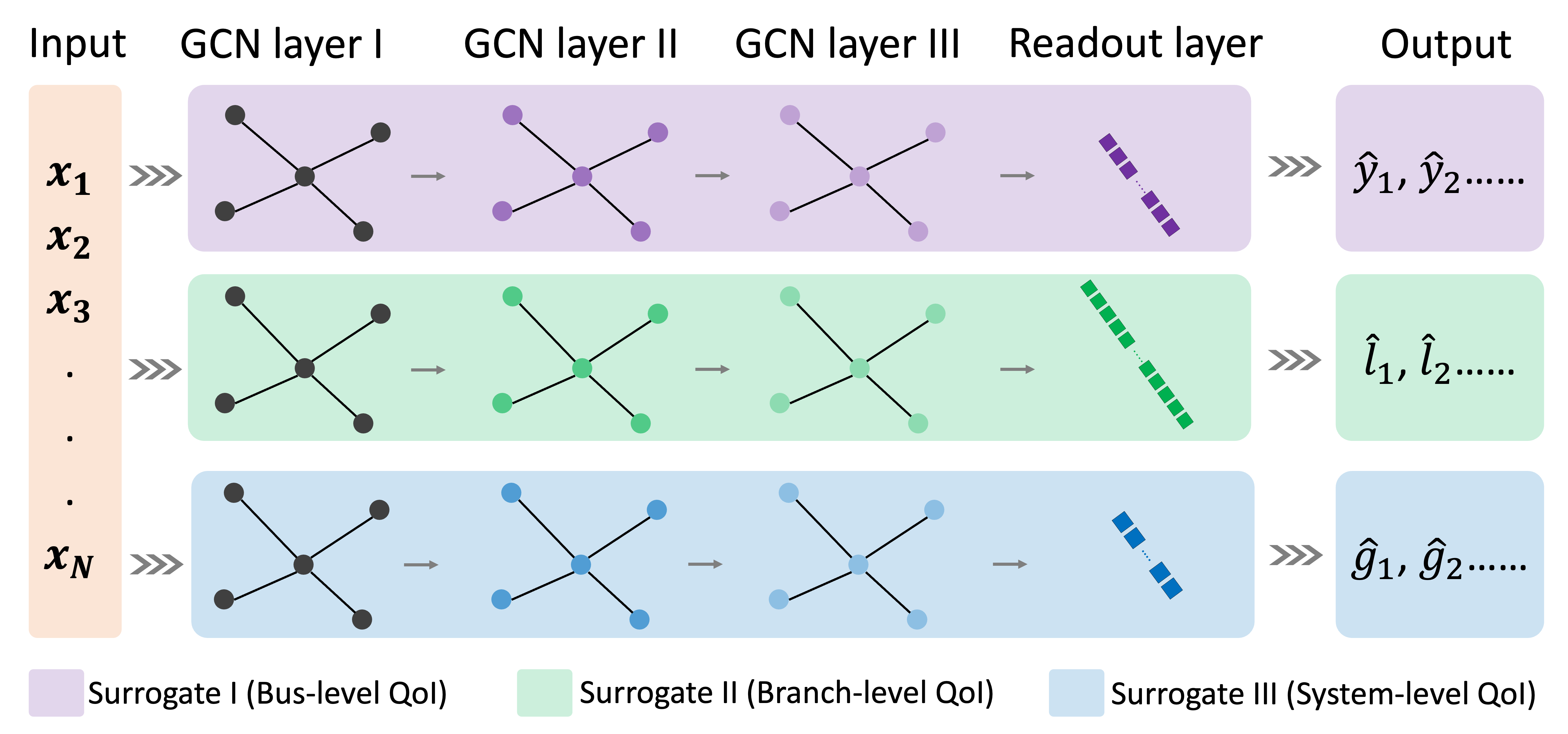
Figure 1: Structure of the three GNN surrogates.

The loss function is constructed using the mean squared error (MSE) loss and a penalty term. The MSE loss is given by:

$$L_{E}=\frac{1}{|\mathcal{V}|}\sum_{i\in\mathcal{V}}(x_{i}-x_{i}^{\ast})^{2},$$ (7)

where $x_{i}^{\ast}$ and $x_{i}$ represent the training data value and predicted value, respectively. A penalty term is added to ensure that the predictions satisfy OPF inequality constraints. The penalty term is expressed as:

$$L_{IE}=\frac{1}{|\mathcal{V}|}\sum_{i\in\mathcal{V}}\zeta_{i}^{2},$$ (8)

where $\zeta_{i}$ is an auxiliary variable defined as:

$$\zeta_{i}=\text{max}\{x_{i}-x^{\rm max}_{i},0\}-\text{min}\{x-x^{\rm min}_{i},0\}$$ (9)

with $x^{\rm min}$ and $x^{\rm max}$ denoting the minimum and maximum allowed value of the QoI. Using weighted averaging, the final loss function can be represented as:

$$L=\omega_{1}L_{E}+\omega_{2}L_{IE}.$$ (10)

Here $\omega_{1}>0$ and $\omega_{2}>0$ are weights and $\omega_{1}+\omega_{2}=1$. Equal weights ($\omega_{1}=\omega_{2}=0.5$) could be used to give equal importance to both constraints.

III-B Training data generation

The stochastic variabilities in the power demand and renewable generation sources (supply) are the main sources of uncertainty in a power grid [41, 7, 8, 4]. The probability distribution that quantifies such variability is not known at the time of training data generation, since it is to be obtained through forecasting for a future time of interest. The training data for the GNN surrogate is therefore generated by considering uniform distributions for the demand $P^{L}_{i},\;\forall\,i\in\mathcal{V}_{L}$ and renewable generation $P^{R}_{i},\;\forall\,i\in\mathcal{V}_{R}$, where $\mathcal{V}_{L}$ and $\mathcal{V}_{R}$ denote the set of load buses and the set of renewable generators, respectively. The lower and upper bounds of the uniform distributions can be decided based on generation capacities and historical load data. The uniform distributions used to generate the training data are uncorrelated. Given a portfolio of stochastic grid variables (i.e., sample values of $P^{L}_{i}\;\forall i\in\mathcal{V}_{L}$ and $P^{R}_{i}\;\forall i\in\mathcal{V}_{R}$), thermal power generation $P^{T}_{i},\;\forall i\in\mathcal{V}_{T}$ and transmission line power flow $I_{i},\;\forall i\in\mathcal{I}$ are uniquely determined by solving the DC OPF problem discussed in Section II-A ($\mathcal{V}_{T}$ and $\mathcal{I}$ represent the set of thermal generators and transmission lines, respectively). The grid state data (thermal generator dispatch and transmission line flows) thus obtained constitute the training data set.

Some of the QoIs needed for reliability and risk assessment, such as operating reserve and load shedding, are not directly available from the OPF solution. Operating reserve refers to the unused generation capacity that can be brought online in the specified time window, whereas load shedding refers to the amount of demand not met by the supply. For a given OPF solution, the operating reserve ($\Theta$) is taken as the residual thermal power generation capacity after satisfying the net load. This can be computed as:

$$\Theta ={\rm max}\left\{\sum_{i\in\mathcal{V}_{T}}P_{i,max}^{T}-\left(\sum_{i\in\mathcal{V}_{L}}P_{i}^{L}-\sum_{i\in\mathcal{V}_{R}}P_{i}^{R}\right),\;\;0\right\},$$ (11)

where $P^{T}_{i,max}$ represents the maximum allowed generation capacity of thermal generators. In case of load shedding, the supply is not able to meet the demand and the OPF solution cannot be obtained. Here, we use the slack bus to provide the required additional power. Power supply from the slack bus ($P_{s}$) is taken as load shedding ($\Psi$):

$$\Psi=\begin{cases}0,\;\;\;\;\text{if}\;P_{s}<0\\ P_{s},\;\;\;\text{if}\;P_{s}\geq 0.\end{cases}$$ (12)

The total cost, which is a system-level QoI, can also be calculated using the thermal generator dispatch and the bid information.

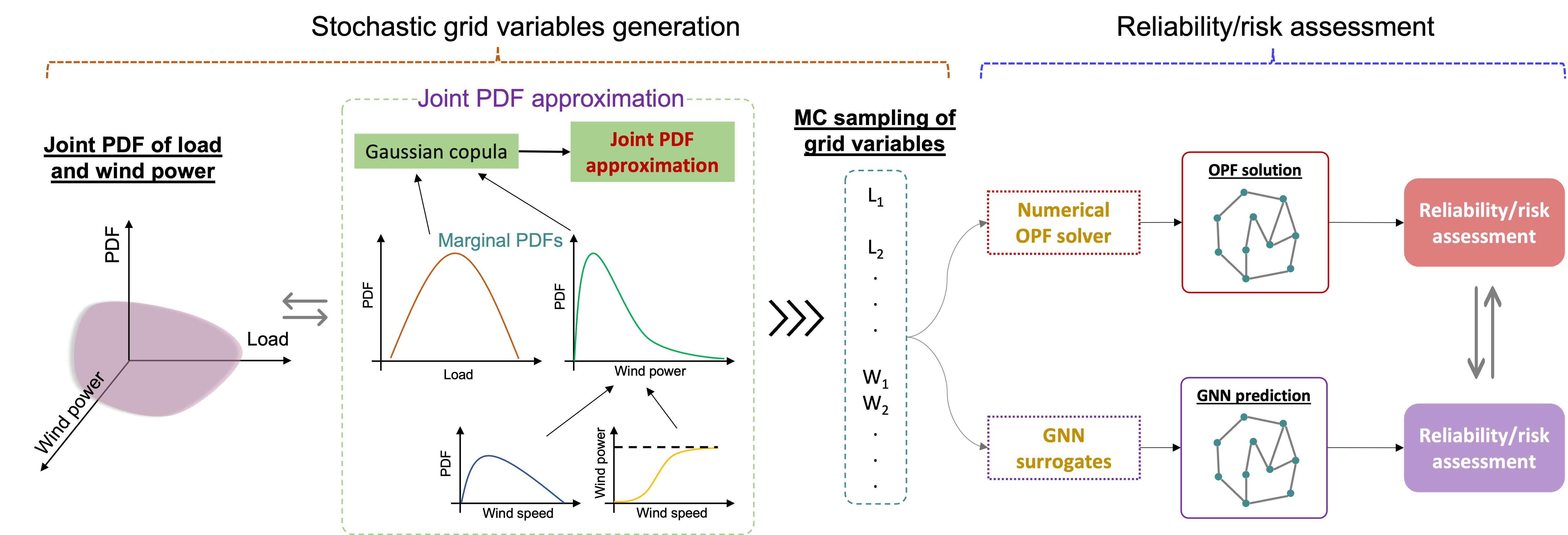
Figure 2: Schematic of Dataset II generation and reliability and risk assessment.

III-C Testing data generation and GNN surrogate evaluation

Two testing datasets (I and II) are used to evaluate the GNN surrogate performance. Dataset I is generated using the same uncorrelated uniform distributions as the training data, but is separate and independent of the training data. This type of test dataset has been used in the majority of the GNN surrogate literature in the power systems domain [7, 4]. Note, however, that the stochastic grid variables in a real power grid do not follow a uniform distribution. Previous studies suggest that the load follows a truncated normal distribution and different renewable generation sources are described by various other probability distributions [5]. Wind power, for instance, is roughly proportional to the cube of wind speed, and wind speed is typically assumed to follow a Weibull distribution [5]. In addition, grid variables are not independent but exhibit correlation [42, 43, 44]. The GNN surrogates are expected to handle such complicated yet more realistic statistical description (probability distributions and dependence structure) of the stochastic grid variables. Therefore, a second test dataset (Dataset II) is generated to test GNN surrogate performance with respect to this key requirement.

To this end, the power grid is partitioned into multiple zones. Each zone contains a certain proportion of load buses, thermal and RES generators. The joint PDF (forecast) of zonal (aggregated) stochastic grid variables, i.e., load and RES power generation, is represented using a Gaussian copula [45] $G_{C}(\mathbf{u})$: $[0,1]^{2s}\rightarrow[0,1]$, for the sake of illustration, as:

$$G_{C}(\mathbf{u})=\Phi_{C}\left(\Phi^{-1}(u_{1}),\Phi^{-1}(u_{2}),...,\Phi^{-1}(u_{2s})\right),$$ (13)

where $s$ is the number of distinct zones, $\mathbf{u}=[u_{1},u_{2},...,u_{2s}]^{T}$ is the random vector containing independent uniform variables, $\Phi$ and $\Phi_{C}$ represent the standard normal CDF and multivariate normal CDF with zero mean and correlation matrix $C$, respectively. In this work, we simply assume a $C$ matrix and use the resulting copula for drawing samples of correlated grid variables ($\mathbf{u}$). Note that in the real-world application of GNN surrogates, samples drawn from the joint forecast PDF of stochastic variables will be used and will therefore correctly incorporate the correlations. Here, the Gaussian copula (with an assumed $C$ matrix) is used only for demonstrating and evaluating GNN-based reliability and risk quantification. Given a sample of $\mathbf{u}$, a sample of correlated stochastic grid variables can be generated as:

$$S_{m}=\Phi_{S_{m}}^{-1}\left(G_{C}(\mathbf{u})\right),\;m=\{1,2,...,2s\},$$ (14)

where $\Phi_{S_{i}}$ represents the marginal CDF of stochastic variable in zone $m$.

Without loss of generality, wind turbines are assumed to be the renewable generators in our illustration. Samples of zonal (aggregated) load ($L_{i}=S_{m},m=1,2,...,s$) and wind generation ($W_{i}=S_{m},m=s+1,s+2,...,2s$) are drawn using the copula. The relative contribution of each load bus/wind turbine is assumed to be a constant in each zone. Consider zone $i$ containing $N_{L}$ load buses and $N_{W}$ wind turbines; then the bus-level load and wind power for zone $i$ are calculated as:

$$\begin{split}L_{i,j}&=r_{i,j}L_{i},\;j=1,2,...,N_{L}\\ W_{i,k}&=q_{i,k}W_{i},\;k=1,2,...,N_{W}\end{split}$$ (15)

where $r_{i,j}$ and $q_{i,k}$ represent the relative contribution of each load bus and wind generator bus to the respective zonal (aggregated) values, and $L_{i}$ and $W_{i}$ denote the aggregated values for zone $i$. Thus it is only necessary to draw samples of $L_{i}$ and $W_{i}$ for each zone, not at each bus. In this manner, a sample of stochastic grid variables with zonal correlation is obtained and used to solve the OPF problem. The procedure used to generate Dataset II is given below:

1. Draw a sample $L_{i}$ and $W_{i}$ for each zone using Eq. 14

2. Calculate load and wind power for load buses and wind generator buses in each zone using Eq. 15.

3. Run a numerical solver (e.g., Pandapower) to get OPF solution corresponding to the given sample of stochastic variables.

4. Repeat Step i to iii multiple times to generate sufficient amount of test data samples for Dataset II.

Note that Dataset II enables the evaluation of GNN surrogate performance for reliability and risk estimation for realistic conditions (correlated grid variables with non-uniform probability distributions). The results from GNN surrogates-based reliability and risk assessment are compared with the ground truth (i.e., OPF-based reliability and risk assessment). The procedure for Dataset II generation and GNN-based reliability and risk assessment evaluation is illustrated in Fig. 2.

III-D Reliability and risk assessment

We consider reserve inadequacy as the failure mode for zonal and system level reliability and risk assessment. At the transmission line level, we consider flow beyond a certain threshold as the failure event. This event is a surrogate for transmission line overloading.

III-D1 Reserve adequacy

To ascertain operating reserve adequacy, we use the minimum reserve requirement (MRR) as the reliability threshold. MRR is typically set as the generation capacity of the single largest generator in the power grid [9]. Therefore, the probability of reserve inadequacy is given by:

$$\mathcal{P}^{S}_{f}(\Phi,\text{MRR})=p(\Phi<\text{MRR}),$$ (16)

and is computed as

$$\mathcal{P}^{S}_{f}(\Phi,\text{MRR})=\frac{1}{M}\sum_{k=1}^{M}V(k),$$ (17)

where $M$ denotes the number of samples, $V(k)=1$ if $\Phi<\text{MRR}$ holds for $k$-th sample and $V(k)=0$ otherwise. Note that MRRs at system and zone levels are considered in this work.

Next, risk is computed as the product of probability of failure and the consequence (monetary cost). A constant consequence cost, $\mathcal{C}^{S}$, is assumed for insufficient reserve; thus the corresponding risk can be calculated as:

$$\Re^{S}(\Phi)=\mathcal{P}^{S}_{f}(\Phi,\text{MRR})\mathcal{C}^{S}.$$ (18)

III-D2 Branch overloading

The risk assessment framework developed by Stover et al. [9] is extended to include reliability and risk quantification for transmission line flow. This extension can help grid operators identify the risk of congestion in the power grid. The electric current $l_{f}$ in one or more branches exceeding a certain threshold $\epsilon$ is considered as a failure event for this purpose. The probability of overloading branch $i$ is defined as:

$$\mathcal{P}^{B}_{f}(i) =p(l_{f,i}\geq\epsilon),$$ (19)

and computed as

$$\mathcal{P}^{B}_{f}(i) =\frac{1}{M}\sum^{M}_{k=1}U_{k}(i),$$ (20)

where $i=\{1,\;2,\;\dots,\;N\}$ with $N$ denoting the number of branches. $U_{k}(i)=1$ if $l_{f}\geq\epsilon$ holds for branch $i$ in the $k$-th sample, otherwise 0. Moreover, the conditional probability of overloading a transmission line $j$, given that transmission line $i$ is overloaded, is also considered. This probability is defined and computed as:

$$\mathcal{P}^{B}_{f}(j|i) =p(l_{f,j}|\Omega_{i})=\frac{1}{|\Omega_{i}|}\sum_{k\in\Omega_{i}}U_{k}(j),$$ (21)

where $j=\{1,\;2,\;\dots,\;N\}$ and $j\neq i$. $\Omega_{i}$ represents the set of samples with $l_{f,i}\geq\epsilon$.

The overall risk of branch overloading, given that branch $i$ is overloaded, can computed by combining Eq. 19 and 21 as:

$$\Re^{B}(i)=\mathcal{P}^{B}_{f}(i)\mathcal{C}_{i}^{B}+\sum^{N}_{j=1,\;j\neq i}\mathcal{P}^{B}_{f}(j|i)\mathcal{C}_{j}^{B}.$$ (22)

where $\mathcal{C}_{i}^{B}$ and $\mathcal{C}_{j}^{B}$ are the consequence costs of overloading of lines $i$ and $j$ respectively. This formula includes the probability of overloading branch $i$ and the conditional probability of overloading any other branch, given that branch $i$ is overloaded; thus it provides a meaningful estimate of overall branch overloading risk. This overall risk can be used by operators to identify the most critical branches in the grid, given a probabilistic forecast of stochastic grid variables.

In summary, this section outlines the procedure of using GNN surrogates to estimate power grid operational reliability and risk. This includes GNN surrogate development, training/test data generation and reliability/ risk quantification. A system-level reliability and risk assessment framework is extended to branch level to account for line flow constraints. The performance of GNN surrogates is evaluated based on both simple (uniform) and complex (realistic) probabilistic forecasts of grid variables.

IV Numerical Example

The proposed GNN surrogate-based reliability and risk assessment method is evaluated on the IEEE Case118 power grid [32] shown in Fig. 3. The power grid consists of 118 buses, 173 branches and 13 transformers and operates at multiple voltages (138 kv, 161 kv and 345 kv). There are 54 generator buses among which 16 are randomly designated as wind turbines in this example. The rest are considered as thermal generators. Renewable energy sources, when they are available, would preferably be fully deployed in a real-world power grid in meeting the demand, due to their low cost and environmental friendliness. In order to enforce this, we always use the wind generator output first towards meeting the demand, and the thermal generators are deployed to satisfy the remaining demand.

For training data and testing dataset I, bus-level load ($P^{L}$) and wind power ($P^{R}$) are randomly drawn from independent and identical uniform distributions $U(50,100)$ (MW) and $U(0,\;100)$ (MW), respectively. Note that the unit of load, wind power as well as power flow are MW unless otherwise specified. Note also that the stochastic variables in Dataset I are independent random variables. A sample of the stochastic variables is given as input to the numerical solver Pandapower to obtain the OPF solution (bus-level, branch-level and system-level QoIs). A total of 1000 samples are generated using the OPF solver (70% for training and 30% for testing). Although these samples share the same grid topology, they are distinct graphs because every node’s feature vectors are different. Supervised learning is used during the training process and the hyper-paramters of the GNN surrogates are carefully tuned to promote training efficiency.

For Dataset II, the power grid is partitioned into three distinct zones (i.e., $s=3$), as shown in Fig. 3. Following the procedure outlined in Section III-C, the joint PDF approximation is established using six ($2s=6$) marginal PDFs (three load and three wind power PDFs) via Eq. 13 and 14 with a correlation matrix assumed as:

$$C=\begin{bmatrix}1&0.7&0.5&0.1&0.05&0.03\\ 0.7&1&0.4&0.02&0.08&0.05\\ 0.5&0.4&1&0.06&0.04&0.1\\ 0.1&0.02&0.06&1&0.3&0.4\\ 0.05&0.08&0.04&0.3&1&0.6\\ 0.03&0.05&0.1&0.4&0.6&1\\ \end{bmatrix}.$$ (23)

Load is assumed to followed a truncated normal (TN) distribution. Wind speed is assumed to follow a Weibull (WB) distribution and wind power is computed from wind speed following the power curve in [5] with rated power generation at 200 MW. The parameters used for these marginal distributions are specified in Table I. For reliability and risk quantification, the following parameters are utilized: $\epsilon=95\%$ of maximum allowable flow capacity, $\text{MRR}=\text{200 MW}$ at both system and zonal level, $\mathcal{C}_{i}^{B}=\$100$ for all $i$, $\mathcal{C}^{S}=\$30,000$ (system) and $\$10,000$ (individual zone).

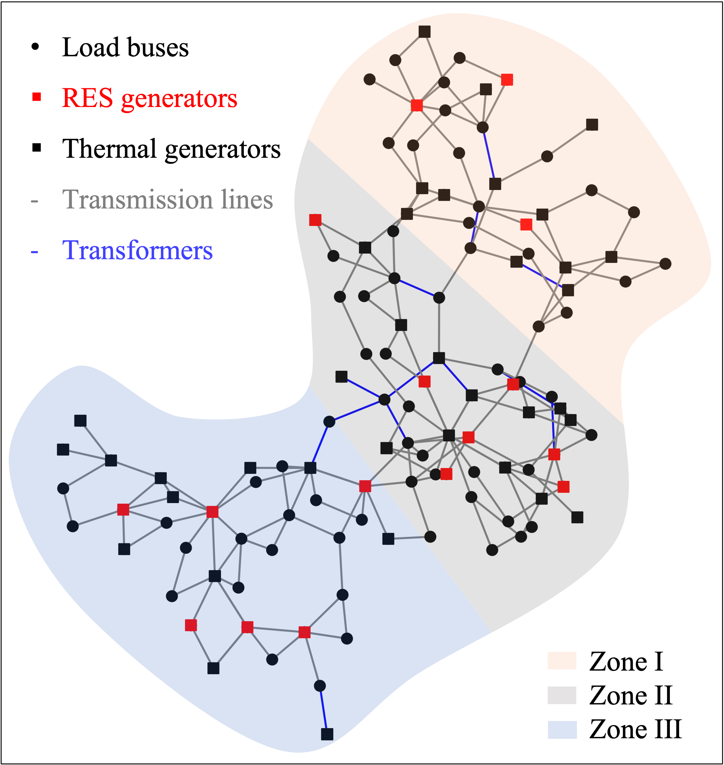
Figure 3: IEEE Case118 power grid.

TABLE I: Parameters used for the truncated normal PDF (load, $MW$) and Weibull PDF (wind speed, $m/s$).

Zone/PDF							Location	Shape	Scale	Left trca.	Right trca.
I	TN	85	–	10	55	115
	WB	1	20	11	–	–
II	TN	90	–	12	55	125
	WB	3	15	8	–	–
III	TN	95	–	15	40	150
	WB	1	10	6	–	–

V Results

The prediction accuracy of GNN surrogates for bus-level and branch-level QoIs is quantified using the mean relative error (MRE) for these predictions with respect to the OPF solution. The one-on-one comparison between GNN prediction and ground truth is provided for system-level QoIs. Accuracy for GNN-based reliability and risk quantification is examined for reserve adequacy at the system and zonal level, while twenty critical (heavily loaded) branches are selected to demonstrate results of branch overloading analysis.

V-A GNN surrogate prediction accuracy

GNN predictions for bus-level and branch-level QoIs are shown in Fig. 4. In terms of active power output in the thermal generator, the MRE is within $\pm 10\%$ for the majority of buses, indicating excellent accuracy of the GNN surrogates. There are a few cases where MRE exceeds $\pm 20\%$, but this is mainly due to lower OPF (true) values that lead to a large relative percentage. In addition, the error bounds for Datasets I and II are nearly the same. These results indicate that the GNN surrogates have learnt the grid’s thermal generator dispatch pattern and they could handle realistic stochastic inputs. GNN surrogates also perform well for power flow prediction in Dataset I, as most of MRE is within $\pm 10\%$. The prediction for Dataset II shows slightly high MRE in some cases. However, for lines with significant amount of power flow ($>$ 100 MW) the error is largely within $\pm 10\%$.

For the system-level QoIs, as shown in Fig. 5, it is found that GNN predictions for load shedding and operating reserve are satisfactorily accurate, whereas those for total cost exhibit slightly higher error when the cost is at the lower end of the spectrum. This, again, is not a major concern, since low cost indicates relatively safer system state. Note that GNN surrogates take $8\times 10^{-4}$ s on average to get one prediction while the numerical OPF solver needs $0.2$ s or more to get one solution. Therefore, GNN surrogates can enable MC sampling-based real-time operational risk estimation by quickly providing thousands of (approximate) OPF solutions, given the updated forecast of the stochastic grid variables.

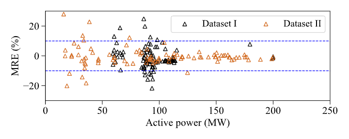
((a)) Bus-level QoI.

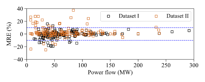
((b)) Branch-level QoI.

Figure 4: GNN surrogates’ performance for bus-level and branch-level QoIs. Blue lines represent $\text{MRE}=\pm 10\%$.

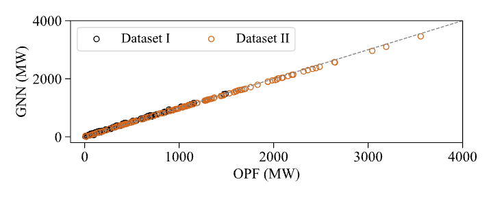
((a)) Load shedding.

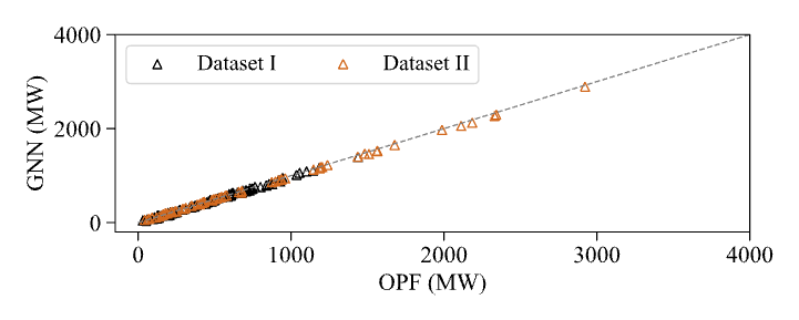
((b)) Operating reserve.

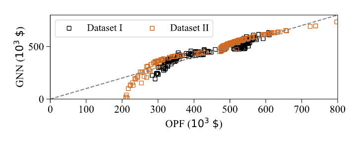
((c)) Total cost.

Figure 5: GNN surrogates performance for system-level QoIs.

V-B GNN surrogates for reliability and risk assessment

V-B1 Reserve adequacy

The results for system level and zonal reserve adequacy are shown in Table II. The GNN surrogate-based prediction of probability of inadequate reserve is very accurate for both Datasets I and II. For the realistic case (Dataset II), zone III is the most vulnerable to reserve shortage with $\mathcal{P}^{s}_{f}=0.2025$, followed by zone I and II at 0.1189 and 0.1554, respectively. However, reserve at the system level seems to be sufficient in most conditions as $\mathcal{P}^{s}_{f}$ is only 0.0566. The corresponding system level and zonal risk estimates are also reported in Table II. For this simple risk model, the GNN-based risk estimate shows excellent agreement with the OPF-based risk estimate.

TABLE II: Reliability and risk quantification in terms of reserve adequacy at the system and zone levels

Zone						Dataset I	Dataset II
	$\mathcal{P}^{S}_{f}$	$\mathcal{\Re^{S}}/\$$	$\mathcal{P}^{S}_{f}$	$\mathcal{\Re^{S}}/\$$
I	OPF	0.5850	5850	0.1189	1189
	GNN	0.5822	5822	0.1084	1084
II	OPF	0.5567	5567	0.1554	1554
	GNN	0.5579	5579	0.1622	1622
III	OPF	0.7667	7667	0.2045	2045
	GNN	0.7759	7759	0.1985	1985
Total	OPF	0.4719	14157	0.0566	1698
	GNN	0.4857	14571	0.0566	1698

V-B2 Branch overloading

Results of branch overloading analysis for Dataset II are shown in Fig. 6. (The results for Dataset I are not included due to page limits). Overall, GNN surrogates provide accurate prediction for the probability of overloading in a transmission line. In particular, $\mathcal{P}^{B}_{f}(i)=1$ for two branches, indicating that they will always approach the maximum allowed capacity and thus operators should give special attention to these lines to ensure the safety of grid operation. There are four branches with $\mathcal{P}^{B}_{f}(i)>0.5$, and they have been identified as such by the GNN surrogate-based assessment. The probability of multiple branch overloading is shown in Fig. 7. Given a heavily loaded critical branch, the conditional probability of overloading all the remaining branches is calculated. Overall, the GNN predictions are in good agreement with the ground truth. It is noticed that overloading does not happen for most branches as the value of $\mathcal{P}^{B}_{f}(j|i)$ is almost zero. Moreover, there are a few branches (e.g., $j={6,7,89,142,150,162,163}$) that experience heavier loading more often than other branches. It is therefore necessary to monitor the flow in these lines during daily operation of the grid.

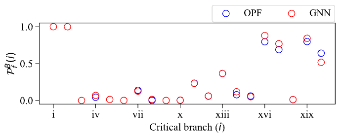
Figure 6: Reliability assessment at branch level (Dataset II). Twenty critical branches are selected to evaluate the GNN surrogate accuracy.

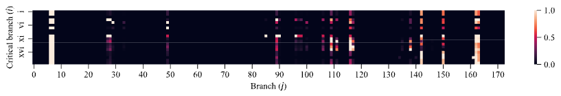
((a)) OPF (Dataset II).

((b)) GNN (Dataset II).

Figure 7: Conditional probability of branch overloading $\mathcal{P}_{f}^{B}(j|i)$.

The overall risk of branch overloading, as defined in Eq. 22, is shown in Fig. 8. It is observed that $\Re^{B}(i)$ ranges between $\$0$ and $\$10,000$. Interestingly, it is found that branches with the highest (marginal) overloading probability (Fig. 6) do not carry the highest overall (system-wide) overloading risk. This indicates that there will be significant risk of overall (system-wide) branch overloading if the branches that rarely experience overloading experience high power flow. The comparison of OPF-based and GNN-based risk estimates indicates that GNN surrogates are sufficiently accurate for predicting this complex (conditional) risk, and can be used for real-time risk assessment.

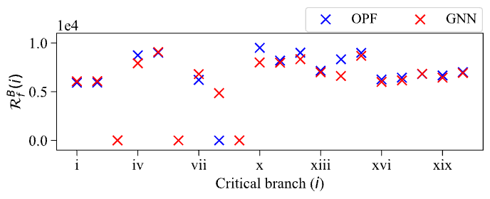
Figure 8: Risk assessment at branch level (Dataset II)

V-B3 GNN surrogate accuracy for different grid forecasts

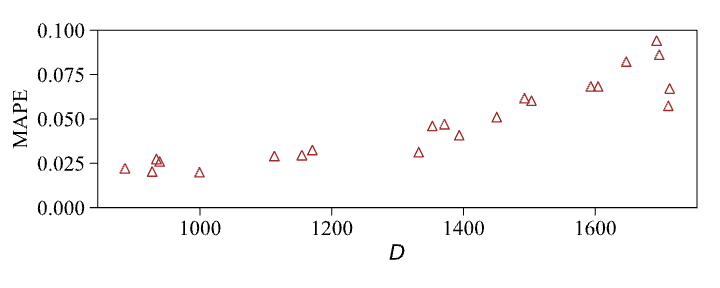
Figure 9: Effect of distance between training and testing data on GNN prediction accuracy.

The GNN surrogate trained using the training data with simple underlying probability distributions (uniform, uncorrelated variables) needs to be exercised for grid variable forecasts that follow more realistic probability distributions (non-uniform, correlated variables) for reliability and risk assessment. It is thus important to quantify the error in reliability or risk estimation as a function of a measure of distance between the training and the forecast distributions. To this end, multiple joint forecast distributions are generated by modifying the marginal distribution parameters in Table I. Samples of correlated grid variables are obtained from each of these distributions and are used to quantify reliability and risk. The similarity between the training data and a candidate (forecast) supply/demand regime (as represented by the corresponding joint probability distributions) is quantified using a statistical distance metric ($D$). If the samples of a random vector ${X}$ are given by $x_{1},x_{2},\dots,x_{n}$ and those of a random vector $Y$ are given by $y_{1},y_{2},\dots,y_{m}$, then $D$ is defined as:

$$D=E[||X-Y||]=\frac{1}{mn}\sum_{i=1}^{n}\sum_{j=1}^{m}||x_{i}-y_{j}||,$$ (24)

where $n$ and $m$ are the number of samples of $X$ and $Y$, respectively, $E$ denotes the expected value, and $||\bullet||$ is a vector norm. A higher value of $D$ indicates a higher degree of dissimilarity between $X$ and $Y$. In the context of GNN surrogate evaluation, $X$ represents training data whereas $Y$ denotes testing data. The (ensemble-based) distance ($D$) between GNN training data and the forecast distribution is computed using Eq. 24. The mean absolute percentage error (MAPE) in the estimation of branch overloading probability (i.e., Fig. 6) for different values of $D$ is shown in Fig. 9. The MAPE $\leq 5$% when $D<1200$, however, the value of MAPE gradually increases after that till it reaches about $10$% for $D=1600$. The methodology used in this exercise could be implemented by grid operators to quantify the error bounds on their GNN-based real-time risk estimates.

VI Conclusion

We investigated the utility of GNN surrogate modeling of the OPF analysis for power grid operational risk assessment. We solved a large number of optimal power flow (OPF) problems to obtain the GNN surrogate training data, and learned multiple GNN surrogates that predict bus-level, branch-level and system-level QoIs. We considered inadequate zonal and system reserve, as well as branch overloading as the relevant failure modes for reliability and risk assessment. The GNN surrogate model performance for predicting the QoI values as well as for quantifying the reliability and risk was assessed using two types of test datasets. The first dataset used simple statistical description (uniform, uncorrelated) for stochastic grid variables (renewable generation and load). This is the prevailing practice in GNN literature on power grids. The second dataset used realistic, complex statistical description of stochastic grid variables. Specifically, we used realistic marginal probability distributions and employed a Gaussian copula to capture the dependence structure of stochastic grid variables. This has not been previously reported in the power grid literature, and GNN surrogate performance evaluation under this complicated joint (forecast) distribution is needed before real-world operational risk assessment of power grids. We demonstrated the proposed GNN surrogate-based reliability and risk estimation methodology on the IEEE Case118 power grid. By comparing OPF-based and GNN-based reliability and risk estimation, we showed that GNN surrogates can provide accurate estimate of the grid’s operational risk at a desired time instant and are also capable of dealing with correlations between variables in distinct zones. We also developed a methodology that could be used to estimate the error in GNN-based reliability and risk estimation as a function of the statistical distance between training data and grid forecast data. The excellent accuracy and lower computational cost of the GNN surrogates as compared to numerical OPF solvers indicate that GNNs can be good surrogates for computationally expensive numerical OPF solvers, and could be deployed for real-time risk assessment.

The proposed methodology has only considered static reliability and risk assessment, for a given unit commitment. It can be extended to capture temporal evolution of grid variables. To that end, it is necessary to examine generator on/off status, ramping rate, wear and tear cost, etc., and consider the change in committed thermal units. In addition, advanced learning methods such as reinforcement learning maybe helpful to improve GNN prediction accuracy, especially for branch-level and system-level QoIs, and thus enhance real-time reliability and risk quantification.

VII Acknowledgement

This work is partly funded by ARPA-E PERFORM award DE-AR0001280. The support is gratefully acknowledged.

References

- [1] M. Milligan, P. Donohoo, D. Lew, E. E. Kirby, B. Holttinen, H. Lannoye, E. Flynn, D. O’malley, M. Miller, and N. Eriksen, “Operating reserves and wind power integration: An international comparison,” National Renewable Energy Lab.(NREL), 2010.
- [2] Ž. B. Rejc and M. Čepin, “Estimating the additional operating reserve in power systems with installed renewable energy sources,” Int. J. Electr. Power Energy Syst., vol. 62, pp. 654–664, Nov. 2014.
- [3] P. J. Heptonstall and R. J. K. Gross, “A systematic review of the costs and impacts of integrating variable renewables into power grids,” Nat. Energy, vol. 6, no. 1, pp. 72–83, Nov. 2020.
- [4] Q. P. Zheng, J. Wang, and A. L. Liu, “Stochastic optimization for unit commitment—a review,” IEEE Trans. Power Syst., vol. 30, no. 4, pp. 1913–1924, Jul. 2015.
- [5] Y.-Y. Hong and G. F. D. G. Apolinario, “Uncertainty in unit commitment in power systems: A review of models, methods, and applications,” Energies, vol. 14, no. 20, p. 6658, Oct. 2021.
- [6] H. Holttinen, M. Milligan, E. Ela, N. Menemenlis, J. Dobschinski, B. Rawn, R. J. Bessa, D. Flynn, E. Gomez Lazaro, and N. Detlefsen, “Methodologies to determine operating reserves due to increased wind power,” in 2013 IEEE Power & Energy Society General Meeting. IEEE, 2013.
- [7] B. Mohandes, M. S. E. Moursi, N. Hatziargyriou, and S. E. Khatib, “A review of power system flexibility with high penetration of renewables,” IEEE Trans. Power Syst., vol. 34, no. 4, pp. 3140–3155, Jul. 2019.
- [8] E. Ela, B. Kirby, E. Lannoye, M. Milligan, D. Flynn, B. Zavadil, and O. Malley, Evolution of operating reserve determination in wind power integration studies. InIEEE PES general meeting. IEEE, 2010.
- [9] O. Stover, P. Karve, and S. Mahadevan, “Reliability and risk metrics to assess operational adequacy and flexibility of power grids,” Reliab. Eng. Syst. Saf., vol. 231, no. 109018, p. 109018, Mar. 2023.
- [10] M. Čepin, Assessment of power system reliability: methods and applications. Springer Science & Business Media, 2011.
- [11] P. Dehghanian and M. Kezunovic, “Probabilistic decision making for the bulk power system optimal topology control,” IEEE Transactions on Smart Grid, vol. 7, no. 4, pp. 2071–2081, 2016.
- [12] V. Bolz, J. RueB, and A. Zell, “Power flow approximation based on graph convolutional networks,” in 2019 18th IEEE International Conference On Machine Learning And Applications (ICMLA). IEEE, Dec. 2019.
- [13] Q. Yang, A. Sadeghi, G. Wang, G. B. Giannakis, and J. Sun, “Power system state estimation using gauss-newton unrolled neural networks with trainable priors,” in 2020 IEEE International Conference on Communications, Control, and Computing Technologies for Smart Grids (SmartGridComm). IEEE, Nov. 2020.
- [14] D. Wang, K. Zheng, Q. Chen, G. Luo, and X. Zhang, “Probabilistic power flow solution with graph convolutional network,” in 2020 IEEE PES Innovative Smart Grid Technologies Europe (ISGT-Europe). IEEE, Oct. 2020.
- [15] P. Xu, Y. Pei, X. Zheng, and J. Zhang, “A simulation-constraint graph reinforcement learning method for line flow control,” in 2020 IEEE 4th Conference on Energy Internet and Energy System Integration (EI2). IEEE, Oct. 2020.
- [16] W. Miao, H. Wu, P. Chen, and J. Jing, “Intelligent auxiliary operation and maintenance system of power communication network based on knowledge graph,” J. Phys. Conf. Ser., vol. 1684, no. 1, p. 012105, Nov. 2020.
- [17] J. Q. James, D. J. Hill, L. Vo, and Y. Hou, “Synchrophasor recovery and prediction: A graph-based deep learning approach,” IEEE Internet of Things Journal, vol. 6, no. 5, pp. 7348–7359, 2019.
- [18] W. L. Hamilton, Graph representation learning. Synthesis Lectures on Artifical Intelligence and Machine Learning. Morgan & Claypool Publishers, 2020, vol. 14.
- [19] W. Liao, B. Bak-Jensen, J. Radhakrishna Pillai, Y. Wang, and Y. Wang, “A review of graph neural networks and their applications in power systems,” J. Mod. Power Syst. Clean Energy, vol. 10, no. 2, pp. 345–360, 2022.
- [20] M. Dezvarei, K. Tomsovic, J. S. Sun, and S. M. Djouadi, “Graph neural network framework for security assessment informed by topological measures,” 2023.
- [21] F. Diehl, “Warm-starting ac optimal power flow with graph neural networks,” in 33rd Conference on Neural Information Processing Systems (NeurIPS 2019), 2019, pp. 1–6.
- [22] N. Sapountzoglou, J. Lago, B. De Schutter, and B. Raison, “A generalizable and sensor-independent deep learning method for fault detection and location in low-voltage distribution grids,” Applied Energy, vol. 276, p. 115299, 2020.
- [23] Y. Benmahamed, M. Teguar, and A. Boubakeur, “Application of svm and knn to duval pentagon 1 for transformer oil diagnosis,” IEEE Transactions on Dielectrics and Electrical Insulation, vol. 24, no. 6, pp. 3443–3451, 2017.
- [24] E. Kabir, S. D. Guikema, and S. M. Quiring, “Predicting thunderstorm-induced power outages to support utility restoration,” IEEE Transactions on Power Systems, vol. 34, no. 6, pp. 4370–4381, 2019.
- [25] A. Al Mamun, M. Sohel, N. Mohammad, M. S. H. Sunny, D. R. Dipta, and E. Hossain, “A comprehensive review of the load forecasting techniques using single and hybrid predictive models,” IEEE Access, vol. 8, pp. 134 911–134 939, 2020.
- [26] P. Xu, Y. Pei, X. Zheng, and J. Zhang, “A simulation-constraint graph reinforcement learning method for line flow control,” in 2020 IEEE 4th Conference on Energy Internet and Energy System Integration (EI2). IEEE, 2020, pp. 319–324.
- [27] H. Yuan, J. Zhang, P. Xu et al., “Study on fast charging demand guid-ance in coupled power-transportation networks based on graph rein-forcement learning,” Power System Technology, vol. 99, pp. 1–9, 2020.
- [28] F. Fusco, B. Eck, R. Gormally, M. Purcell, and S. Tirupathi, “Knowledge-and data-driven services for energy systems using graph neural networks,” in 2020 IEEE International Conference on Big Data (Big Data). IEEE, 2020, pp. 1301–1308.
- [29] J. Huang, L. Guan, Y. Su, H. Yao, M. Guo, and Z. Zhong, “Recurrent graph convolutional network-based multi-task transient stability assessment framework in power system,” IEEE Access, vol. 8, pp. 93 283–93 296, 2020.
- [30] W. Miao, H. Wu, P. Chen, and J. Jing, “Intelligent auxiliary operation and maintenance system of power communication network based on knowledge graph,” in Journal of Physics: Conference Series, vol. 1684, no. 1. IOP Publishing, 2020, p. 012105.
- [31] M. L. Rizzo and G. J. Székely, “Energy distance,” wiley interdisciplinary reviews: Computational statistics, vol. 8, no. 1, pp. 27–38, 2016.
- [32] O. D. Montoya, W. Gil-González, and A. Garces, “Sequential quadratic programming models for solving the OPF problem in DC grids,” Electric Power Syst. Res., vol. 169, pp. 18–23, Apr. 2019.
- [33] A. S. Zamzam and K. Baker, “Learning optimal solutions for extremely fast AC optimal power flow,” in 2020 IEEE International Conference on Communications, Control, and Computing Technologies for Smart Grids (SmartGridComm). IEEE, Nov. 2020.
- [34] C. Duan, W. Fang, L. Jiang, L. Yao, and J. Liu, “Distributionally robust chance-constrained approximate AC-OPF with wasserstein metric,” IEEE Trans. Power Syst., vol. 33, no. 5, pp. 4924–4936, Sep. 2018.
- [35] X. Pan, M. Chen, T. Zhao, and S. H. Low, “Deepopf: A feasibility-optimized deep neural network approach for ac optimal power flow problems,” 2020.
- [36] A. G. Bakirtzis and P. N. Biskas, “A decentralized solution to the dc-opf of interconnected power systems,” IEEE Transactions on Power Systems, vol. 18, no. 3, pp. 1007–1013, 2003.
- [37] D. Deka and S. Misra, “Learning for dc-opf: Classifying active sets using neural nets,” in 2019 IEEE Milan PowerTech. IEEE, 2019, pp. 1–6.
- [38] T. N. Kipf and M. Welling, “Semi-supervised classification with graph convolutional networks,” 2016.
- [39] C. Gao, X. Wang, X. He, and Y. Li, “Graph neural networks for recommender system,” in Proceedings of the Fifteenth ACM International Conference on Web Search and Data Mining, 2022, pp. 1623–1625.
- [40] A. Chaudhary, H. Mittal, and A. Arora, “Anomaly detection using graph neural networks,” in 2019 international conference on machine learning, big data, cloud and parallel computing (COMITCon). IEEE, 2019, pp. 346–350.
- [41] H. Holttinen, M. Milligan, E. Ela, N. Menemenlis, J. Dobschinski, B. Rawn, R. J. Bessa, D. Flynn, E. Gomez Lazaro, and N. Detlefsen, “Methodologies to determine operating reserves due to increased wind power,” in 2013 IEEE Power & Energy Society General Meeting. IEEE, 2013.
- [42] G. Li, C.-C. Liu, C. Mattson, and J. Lawarree, “Day-ahead electricity price forecasting in a grid environment,” IEEE Trans. Power Syst., vol. 22, no. 1, pp. 266–274, Feb. 2007.
- [43] M. Aien, M. Fotuhi-Firuzabad, and M. Rashidinejad, “Probabilistic optimal power flow in correlated hybrid wind–photovoltaic power systems,” IEEE Trans. Smart Grid, vol. 5, no. 1, pp. 130–138, Jan. 2014.
- [44] M. B. Amor, E. Billette de Villemeur, M. Pellat, and P.-O. Pineau, “Influence of wind power on hourly electricity prices and GHG (greenhouse gas) emissions: Evidence that congestion matters from ontario zonal data,” Energy (Oxf.), vol. 66, pp. 458–469, Mar. 2014.
- [45] J. Tastu, P. Pinson, and H. Madsen, “Space-time scenarios of wind power generation produced using a gaussian copula with parametrized precision matrix,” Technical University of Denmark, Tech. Rep., 2013.