BOB: Bayesian Optimized Bootstrap
with Applications to Gaussian Mixture Models

Abstract

Sampling from the joint posterior distribution of Gaussian mixture models (GMMs) via standard Markov chain Monte Carlo (MCMC) imposes several computational challenges, which have prevented a broader full Bayesian implementation of these models. A growing body of literature has introduced the Weighted Likelihood Bootstrap and the Weighted Bayesian Bootstrap as alternatives to MCMC sampling. The core idea of these methods is to repeatedly compute maximum a posteriori (MAP) estimates on many randomly weighted posterior densities. These MAP estimates then can be treated as approximate posterior draws. Nonetheless, a central question remains unanswered: How to select the distribution of the random weights under arbitrary sample sizes. Thus, we introduce the Bayesian Optimized Bootstrap (BOB), a computational method to automatically select the weights distribution by minimizing, through Bayesian Optimization, a black-box and noisy version of the reverse KL divergence between the Bayesian posterior and an approximate posterior obtained via random weighting. Our proposed method allows for uncertainty quantification, approximate posterior sampling, and embraces recent developments in parallel computing. We show that BOB outperforms competing approaches in recovering the Bayesian posterior, while retaining key theoretical properties from existing methods. BOB’s performance is demonstrated through extensive simulations, along with real-world data analyses.

Keywords: Weighted Bayesian Bootstrap, Bayesian Optimization, Multimodal Posterior Sampling, Finite Mixture Models, Monte Carlo Methods, Parallel Computing.

1 Introduction

Gaussian Mixture Models (GMMs) are powerful and flexible tools, which turn up naturally when the population of sampling units consists of homogeneous clusters or subgroups (Van Havre et al.,, 2015), and can be applied in a wide range of scientific problems including model-based clustering (Fraley and Raftery,, 2002; Grazian,, 2023), density estimation (Izenman and Sommer,, 1988), or as flexible semi-parametric model-based approaches for analyzing complex data (Omori et al.,, 2007). It is no surprise, then, that uncertainty quantification to infer properties of a population of interest based on mixture models is now a crucial and important area of statistical research (Wade and Ghahramani,, 2018), and a natural way to quantify uncertainty in mixture models is through Bayesian methods by specifying a sampling model and a prior distribution (Ni et al.,, 2020).

Motivation. Despite the flexibility and wide applicability of GMMs, the large computational costs of Bayesian inference have prevented a broader full Bayesian implementation of these models. For instance, one could sample from the posterior distribution of GMMs via standard Markov chain Monte Carlo (MCMC). Nonetheless, since the log-likelihood function is non-concave, the resulting posterior might be multimodal. The multimodality of the posterior, combined with the serial nature of MCMC algorithms, results in a sampler that might get trapped in local regions of high posterior density, failing to explore the entire parameter space and leading to mixing limitations between posterior modes (Celeux et al.,, 2000; Fong et al.,, 2019). Moreover, in the context of mixture models, MCMC algorithms scale poorly to large datasets (Ni et al.,, 2020) and their serial nature has prevented the adoption of recent developments in parallel computing (Newton et al.,, 2021; Pompe,, 2021), exacerbating even further the computational limitations of these methods. Thus, in order to maintain the challenged Bayesian inferential paradigm relevant throughout the era of big data, new and refined posterior samplers are still required.

Related Work. This research joins a growing body of literature, dating back to 1994 when Newton and Raftery, proposed the Weighted Likelihood Bootstrap (WLB) as an alternative to MCMC. The main idea behind WLB is to generate approximate posterior draws by independently maximizing a series of randomly weighted log-likelihood functions. WLB, however, does not naturally incorporate any prior information in the sampling procedure. With this in mind, researchers have been recently extending the WLB framework to accommodate prior information by weighting not only the likelihood but also the prior. A few examples include the Weighted Bayesian Bootstrap, or WBB (Newton et al.,, 2021; Ng and Newton,, 2022) and the Bayesian Bootstrap spike-and-slab Lasso (Nie and Ročková, 2023a, ). In the context of generalized Bayesian analysis and model misspecification, we can find the loss-likelihood Bootstrap (Lyddon et al.,, 2019), the Posterior Bootstrap (Fong et al.,, 2019; Pompe,, 2021) and the Deep Bayesian Bootstrap (Nie and Ročková, 2023b, ).

Our Contribution. Up until now, one key question has not been addressed: how to select the distribution of the random weights under arbitrary—especially under small to medium—sample sizes. Few analyses have been proposed from the lenses of asymptotic theory but, to the best of our knowledge, the core of this question remains unanswered. Indeed, as discussed by Newton and Raftery, (1994) and Nie and Ročková, 2023b , “no general recipe (to select the weights distribution) yet exists.” Thus, in this work we develop the Bayesian Optimized Bootstrap (BOB), a computational approach to automatically select the distribution of the random weights by minimizing a black-box and noisy version of the reverse Kullback–Leibler (KL) divergence between the Bayesian posterior and an approximate posterior obtained via random weighting. However, since we do not have access to a closed-form expression for such a noisy, and expensive to evaluate, divergence, the minimization is carried out via Bayesian Optimization, or BO (and thus the name BOB), as BO is one of the most efficient approaches to optimize a black-box objective with little evaluations (Jones et al.,, 1998; Jones,, 2001). We show that BOB leads to a better approximation of the Bayesian posterior, it allows for uncertainty quantification, and, unlike MCMC, it is trivially parallelizable.

Article Outline. The rest of this article is organized as follows. Section 2 revisits WBB and describes how a full Bayesian implementation of GMMs can be carried out within a WBB framework. In Section 3 we formally introduce BOB and draw connections with existing Bootstrap approaches. Simulation exercises are carried out in Section 4. In section 5, we demonstrate the applicability of BOB on real-world data. We conclude with a discussion in Section 6.

2 Revisiting Weighted Bayesian Bootstrap

2.1 Problem Setup

For our sampling model, let $\left\{\mathbf{y}_{1},\dots,\mathbf{y}_{n}\right\}$ be a random sample from a Gaussian Mixture with $K$ components. More precisely, let the density of $\mathbf{y}_{i}\in\mathbb{R}^{d}$, for $i\in\{1\,\dots,n\}$, be

$$p\bigl{(}\mathbf{y}_{i}\bigl{|}\left\{\pi_{k},\boldsymbol{\mu}_{k},\boldsymbol{\Sigma}_{k}\right\}_{k=1}^{K}\bigr{)}=\sum_{k=1}^{K}\pi_{k}\varphi\left(\mathbf{y}_{i};\,\boldsymbol{\mu}_{k},\boldsymbol{\Sigma}_{k}\right),$$ (1)

where $\pi_{k}\in[0,1]$ is the weight of component $k$ so that $\sum_{k=1}^{K}\pi_{k}=1$, $K\geq 2$ is a known integer, $\varphi(\cdot\,;\,\boldsymbol{\mu}_{k},\boldsymbol{\Sigma}_{k})$ denotes the Gaussian density with mean vector $\boldsymbol{\mu}_{k}\in\mathbb{R}^{d}$ and covariance matrix $\boldsymbol{\Sigma}_{k}\in\mathbb{M}_{+}^{d}$, and $\mathbb{M}_{+}^{d}$ denotes the set of symmetric positive semidefinite matrices of size $d\times d$. Additionally, let us define the latent indicator variables $z_{ik}=\mathbbm{1}\{i\text{-th obs. is drawn from the }k\text{-th component}\}$ so that $\mathbf{z}_{i}=(z_{i1},\dots,z_{iK})^{\prime}\sim\mathcal{M}(1;\left\{\pi_{k}\right\}_{k=1}^{K})$, where $\mathcal{M}$ denotes the multinomial distribution. Then, the joint distribution of $\mathbf{Y}=(\mathbf{y}_{1}^{\prime},\dots,\mathbf{y}_{n}^{\prime})^{\prime}\in\mathbb{R}^{n\times d}$ and $\mathbf{Z}=(\mathbf{z}_{1}^{\prime},\dots,\mathbf{z}_{n}^{\prime})^{\prime}\in\{0,1\}^{n\times K}$ would be given by

$$p\bigl{(}\mathbf{Y},\mathbf{Z}\bigl{|}\left\{\pi_{k},\boldsymbol{\mu}_{k},\boldsymbol{\Sigma}_{k}\right\}_{k=1}^{K}\bigr{)}=\prod_{i=1}^{n}\prod_{k=1}^{K}\left(\pi_{k}\varphi\left(\mathbf{y}_{i};\,\boldsymbol{\mu}_{k},\boldsymbol{\Sigma}_{k}\right)\right)^{z_{ik}}.$$ (2)

For our prior specification, let $\boldsymbol{\mu}_{k}|\boldsymbol{\Sigma}_{k}\sim\mathcal{N}(\boldsymbol{\beta}_{k},\,\boldsymbol{\Sigma}_{k}/\lambda_{k})$, $\boldsymbol{\Sigma}_{k}\sim\mathcal{IW}(\nu_{k},\,\boldsymbol{\Psi}_{k})$, and $\boldsymbol{\pi}\sim\mathcal{D}(a_{1},\dots,a_{K})$, which corresponds to a normal-inverse-Wishart prior for $\boldsymbol{\mu}_{k}$ and $\boldsymbol{\Sigma}_{k}$, and a Dirichlet prior for the mixture proportions $\boldsymbol{\pi}=(\pi_{1},\dots,\pi_{K})^{\prime}$. Additionally, let $\boldsymbol{\theta}=\left\{\pi_{k},\boldsymbol{\mu}_{k},\boldsymbol{\Sigma}_{k}\right\}_{k=1}^{K}\in\boldsymbol{\Theta}$ be the collection of all model parameters so that, under the sampling distribution and priors introduced above, the joint Bayesian posterior would be, up to a proportionality constant, given by

$$p(\boldsymbol{\theta},\mathbf{Z}|\mathbf{Y})\propto p(\boldsymbol{\pi})\prod_{k=1}^{K}\left\{p(\boldsymbol{\Sigma}_{k})p(\boldsymbol{\mu}_{k}|\boldsymbol{\Sigma}_{k})\prod_{i=1}^{n}p(\mathbf{y}_{i}|\boldsymbol{\mu}_{k},\boldsymbol{\Sigma}_{k},z_{ik})p(z_{ik}|\pi_{k})\right\}.$$ (3)

2.2 Posterior Sampling via Random Weighting

We now illustrate how one can approximately sample from the joint posterior in (3) via WBB. Following Newton et al., (2021), WBB can be summarized in three simple steps:

Step 1: Start by sampling random weights $\mathbf{u}=(u_{1},\dots,u_{n})^{\prime}$ from some weight distribution $F_{u}$ and construct the re-weighted log-density of $\mathbf{Y}$ and $\mathbf{Z}$ as

$$\log p_{u}\left(\mathbf{Y},\mathbf{Z}|\boldsymbol{\theta}\right)=\sum_{i=1}^{n}u_{i}\left\{\sum_{k=1}^{K}z_{ik}\left[\log\pi_{k}+\log\varphi(\mathbf{y}_{i};\,\boldsymbol{\mu}_{k},\boldsymbol{\Sigma}_{k})\right]\right\}.$$ (4)

Step 2: Sample $\tilde{\mathbf{u}}=(\tilde{u}_{\pi},\tilde{u}_{\mu_{1}},\dots,\tilde{u}_{\mu_{K}},\tilde{u}_{\Sigma_{1}},\dots,\tilde{u}_{\Sigma_{K}})^{\prime}$ from some weight distribution $F_{\tilde{u}}$ and construct the re-weighted log-prior density as

$$\begin{split}\log p_{\tilde{u}}(\boldsymbol{\theta})&\propto\sum_{k=1}^{K}\Biggl{\{}\tilde{u}_{\pi}\left(a_{k}-1\right)\log\pi_{k}-\tilde{u}_{\Sigma_{k}}\left[\left(\frac{\nu_{k}+d}{2}+1\right)\log|\boldsymbol{\Sigma}_{k}|+\frac{\operatorname{tr}\left(\boldsymbol{\Psi}_{k}\boldsymbol{\Sigma}_{k}^{-1}\right)}{2}\right]\\ &\qquad\qquad-\tilde{u}_{\mu_{k}}\left[\frac{\lambda_{k}}{2}(\boldsymbol{\mu}_{k}-\boldsymbol{\beta}_{k})^{\prime}\boldsymbol{\Sigma}_{k}^{-1}(\boldsymbol{\mu}_{k}-\boldsymbol{\beta}_{k})\right]\Biggr{\}}.\end{split}$$ (5)

Step 3: By marginalizing $\mathbf{Z}$ out of equation (4), one would have that $\log p_{u}\left(\mathbf{Y}\left|\boldsymbol{\theta}\right.\right)=\log\left(\sum_{Z}p_{u}\left(\mathbf{Y},\mathbf{Z}\left|\boldsymbol{\theta}\right.\right)\right)$ and the re-weighted log-posterior of $\boldsymbol{\theta}$ would be, up to an additive constant, given by $\log p_{u}(\boldsymbol{\theta}|\mathbf{Y})\propto\log p_{u}\left(\mathbf{Y}\left|\boldsymbol{\theta}\right.\right)+\log p_{\tilde{u}}(\boldsymbol{\theta})$. WBB proceeds to maximize this posterior density seeking

$$\boldsymbol{\theta}^{*}=\operatorname*{arg\,max}_{\boldsymbol{\theta}\in\boldsymbol{\Theta}}\left\{\log p_{u}(\boldsymbol{\theta}|\mathbf{Y})\right\}.$$ (6)

Under a standard Bayesian framework, the randomness in $\boldsymbol{\theta}$ arises from treating it as a random variable with a prior distribution. On the other hand, as discussed in Nie and Ročková, 2023b , $\boldsymbol{\theta}^{*}$ can be seen as an estimator, where, given the data, the only source of randomness comes from the random weights. Thus, by fixing the data $\mathbf{Y}$ and repeating steps 1 - 3 many times, one would have approximate posterior draws $\{\boldsymbol{\theta}^{*}_{(s)}\}_{s\in\mathbb{N}}$. This idea is attractive as optimizing can be easier and less computationally intensive than sampling from an intractable posterior. Note, additionally, that the random weights are independent across iterations, and thus, $\boldsymbol{\theta}^{*}_{(s)}$ and $\boldsymbol{\theta}^{*}_{(s^{\prime})}$, for $s\neq s^{\prime}$, are also independent and could be sampled in parallel. Moreover, Bootstrap-based posterior samplers do not require costly tuning runs, burn-in periods, or convergence diagnostics as in traditional MCMC (Fong et al.,, 2019; Pompe,, 2021), making random weighting an attractive alternative for posterior sampling.

Nonetheless, performing the joint optimization in (6) is still a challenge on its own, especially in light of the non-concavity of $\log p_{u}(\boldsymbol{\theta}|\mathbf{Y})$. Thus, we treat the latent indicator variables, $\mathbf{Z}$, as missing data and use an expectation-maximization (EM) algorithm (Dempster et al.,, 1977) to solve (6).

2.3 Randomly Weighted Expectation-Maximization

2.3.1 Expectation-Step

We start by computing the expected value of $\mathbf{Z}$, conditional on $\mathbf{Y}$, $\mathbf{u}$ and $\boldsymbol{\theta}^{(t)}$, where $\boldsymbol{\theta}^{(t)}$ is the current value of $\boldsymbol{\theta}$ within the EM algorithm. By Bayes’ rule, we have that

$$\begin{split}\mathbb{E}\left[z_{ik}|\boldsymbol{\theta}^{(t)},\mathbf{Y},\mathbf{u}\right]&=\frac{\exp\left\{u_{i}\left[\log\mathbb{P}\left(z_{ik}=1|\pi_{k}^{(t)}\right)+\log\varphi\left(\mathbf{y}_{i};\,\boldsymbol{\mu}_{k}^{(t)},\boldsymbol{\Sigma}_{k}^{{(t)}}\right)\right]\right\}}{\sum_{r=1}^{K}\exp\left\{u_{i}\left[\log\mathbb{P}\left(z_{ir}=1|\pi_{r}^{(t)}\right)+\log\varphi\left(\mathbf{y}_{i};\,\boldsymbol{\mu}_{r}^{(t)},\boldsymbol{\Sigma}_{r}^{{(t)}}\right)\right]\right\}}\\ &=\frac{\left[\pi_{k}^{(t)}\varphi\left(\mathbf{y}_{i};\,\boldsymbol{\mu}_{k}^{(t)},\boldsymbol{\Sigma}_{k}^{{(t)}}\right)\right]^{u_{i}}}{\sum_{r=1}^{K}\left[\pi_{r}^{(t)}\varphi\left(\mathbf{y}_{i};\,\boldsymbol{\mu}_{r}^{(t)},\boldsymbol{\Sigma}_{r}^{{(t)}}\right)\right]^{u_{i}}}=q_{ik}.\end{split}$$ (7)

2.3.2 Maximization-Step

In the maximization step, we then maximize the following surrogate objective function with respect to $\boldsymbol{\theta}\in\boldsymbol{\Theta}$.

$$\begin{split}\mathbb{E}\left[\log p_{u}(\boldsymbol{\theta},\mathbf{Z}|\mathbf{Y})|\boldsymbol{\theta}^{(t)}\right]=-\frac{1}{2}\sum_{i=1}^{n}u_{i}\left\{\sum_{k=1}^{K}q_{ik}\left[\log|\boldsymbol{\Sigma}_{k}|+\left(\mathbf{y}_{i}-\boldsymbol{\mu}_{k}\right)^{\prime}\boldsymbol{\Sigma}_{k}^{-1}\left(\mathbf{y}_{i}-\boldsymbol{\mu}_{k}\right)\right]\right\}\qquad\;\;\\ -\sum_{k=1}^{K}\Biggl{\{}\tilde{u}_{\mu_{k}}\left[\frac{\lambda_{k}}{2}(\boldsymbol{\mu}_{k}-\boldsymbol{\beta}_{k})^{\prime}\boldsymbol{\Sigma}_{k}^{-1}(\boldsymbol{\mu}_{k}-\boldsymbol{\beta}_{k})\right]+\tilde{u}_{\Sigma_{k}}\left[\left(\frac{\nu_{k}+d}{2}+1\right)\log|\boldsymbol{\Sigma}_{k}|+\frac{\operatorname{tr}\left(\boldsymbol{\Psi}_{k}\boldsymbol{\Sigma}^{-1}_{k}\right)}{2}\right]\qquad\\ -\left[\tilde{a}_{k}-1+\sum_{i=1}^{n}u_{i}q_{ik}\right]\log\pi_{k}\Biggr{\}},\qquad\qquad\qquad\qquad\qquad\qquad\qquad\end{split}$$ (8)

where $\tilde{a}_{k}=(a_{k}-1)\tilde{u}_{\pi}+1$. As we will illustrate shortly, the objective in (8) leads to well-known maximization problems, which can be solved relatively cheaply.

Proposition 1.

Let us define $\tilde{n}_{k}=\sum_{i=1}^{n}u_{i}q_{ik}$, $\tilde{\lambda}_{k}=\tilde{u}_{\mu_{k}}\lambda_{k}$, $\tilde{\boldsymbol{\Psi}}_{k}=\tilde{u}_{\Sigma_{k}}\boldsymbol{\Psi}_{k}$, $\tilde{\nu}_{k}=\tilde{u}_{\Sigma_{k}}(\nu_{k}+d+2)-2-d$, $\tilde{\bar{\mathbf{y}}}_{k}=(\tilde{n}_{k})^{-1}\sum_{i=1}^{n}(u_{i}q_{ik})\mathbf{y}_{i}$ and $\tilde{\mathbf{S}}_{k}=\sum_{i=1}^{n}(u_{i}q_{ik})(\mathbf{y}_{i}-\tilde{\bar{\mathbf{y}}}_{k})(\mathbf{y}_{i}-\tilde{\bar{\mathbf{y}}}_{k})^{\prime}$, for all $k\in\{1,\dots,K\}$. Additionally, let $\bar{\boldsymbol{\beta}}_{k}=\tilde{\lambda}_{k}/(\tilde{\lambda}_{k}+\tilde{n}_{k})\boldsymbol{\beta}_{k}+\tilde{n}_{k}/(\tilde{\lambda}_{k}+\tilde{n}_{k})\tilde{\bar{\mathbf{y}}}_{k}$, $\bar{\boldsymbol{\Psi}}_{k}=(\tilde{\boldsymbol{\Psi}}_{k}+\tilde{\mathbf{S}}_{k}+\tilde{\lambda}_{k}\tilde{n}_{k}/(\tilde{\lambda}_{k}+\tilde{n}_{k})(\tilde{\bar{\mathbf{y}}}_{k}-\boldsymbol{\beta}_{k})(\tilde{\bar{\mathbf{y}}}_{k}-\boldsymbol{\beta}_{k})^{\prime})$, $\bar{\lambda}_{k}=\tilde{\lambda}_{k}+\tilde{n}_{k}$, and $\bar{\nu}_{k}=\tilde{\nu}_{k}+\tilde{n}_{k}$. Then, the update of $\boldsymbol{\mu}_{k}$ and $\boldsymbol{\Sigma}_{k}$ would be given by

$$\bigl{(}\boldsymbol{\mu}_{k}^{(t+1)},\boldsymbol{\Sigma}_{k}^{(t+1)}\bigr{)}=\operatorname*{arg\,max}_{\begin{subarray}{c}\boldsymbol{\mu}_{k},\,\boldsymbol{\Sigma}_{k}\end{subarray}}\bigl{\{}h(\boldsymbol{\mu}_{k},\boldsymbol{\Sigma}_{k})\bigr{\}},$$ (9)

where

$$h(\boldsymbol{\mu}_{k},\boldsymbol{\Sigma}_{k})=-\left(\frac{\bar{\nu}_{k}+d}{2}+1\right)\log|\boldsymbol{\Sigma}_{k}|-\frac{1}{2}\operatorname{tr}\left(\bar{\boldsymbol{\Psi}}_{k}\boldsymbol{\Sigma}_{k}^{-1}\right)-\frac{\bar{\lambda}_{k}}{2}(\boldsymbol{\mu}_{k}-\bar{\boldsymbol{\beta}}_{k})^{\prime}\boldsymbol{\Sigma}_{k}^{-1}(\boldsymbol{\mu}_{k}-\bar{\boldsymbol{\beta}}_{k}).$$

Details on the derivation of $h:\mathbb{R}^{d}\times\mathbb{M}_{+}^{d}\rightarrow\mathbb{R}$ are presented in the supplementary materials. To optimize $h$, we make use of a two-stage procedure in which we first update $\boldsymbol{\Sigma}_{k}$ and then update $\boldsymbol{\mu}_{k}$.

Update $\boldsymbol{\Sigma}_{k}$: Start by noting that $\boldsymbol{\Sigma}_{k}\mapsto\log\int_{\mathbb{R}^{d}}\exp(h(\boldsymbol{\mu}_{k},\boldsymbol{\Sigma}_{k}))d\boldsymbol{\mu}_{k}$ is a monotone transformation of $\boldsymbol{\Sigma}_{k}\mapsto h(\boldsymbol{\mu}_{k},\boldsymbol{\Sigma}_{k})$ (Schilling,, 2017, Ch. 9). Thus, optimizing (9) with respect to $\boldsymbol{\Sigma}_{k}$ yields

$$\boldsymbol{\Sigma}_{k}^{(t+1)}=\operatorname*{arg\,max}_{\boldsymbol{\Sigma}_{k}\in\mathbb{M}_{+}^{d}}\left\{-\frac{\bar{\nu}_{k}+d+1}{2}\log|\boldsymbol{\Sigma}_{k}|-\frac{1}{2}\operatorname{tr}\left(\bar{\boldsymbol{\Psi}}_{k}\boldsymbol{\Sigma}_{k}^{-1}\right)\right\}.$$ (10)

One can identify the solution to (10) as the mode of an $\mathcal{IW}(\bar{\nu}_{k},\,\bar{\boldsymbol{\Psi}}_{k})$ distribution. This is,

$$\boldsymbol{\Sigma}_{k}^{(t+1)}=\frac{\bar{\boldsymbol{\Psi}}_{k}}{\bar{\nu}_{k}+d+1}.$$ (11)

Update $\boldsymbol{\mu}_{k}$: Again, note that $\boldsymbol{\mu}_{k}\mapsto\int_{\mathbb{M}_{+}^{d}}\exp(h(\boldsymbol{\mu}_{k},\boldsymbol{\Sigma}_{k}))d\boldsymbol{\Sigma}_{k}$ is a monotone transformation of $\boldsymbol{\mu_{k}}\mapsto h(\boldsymbol{\mu}_{k},\boldsymbol{\Sigma}_{k})$, and so, optimizing (9) with respect to $\boldsymbol{\mu}_{k}$ reduces to

$$\boldsymbol{\mu}_{k}^{(t+1)}=\operatorname*{arg\,max}_{\boldsymbol{\mu}_{k}\in\mathbb{R}^{d}}\left\{\left[1+\left(\bar{\lambda}_{k}(\bar{\nu}_{k}-d+1)^{2}\right)^{-1}(\boldsymbol{\mu}_{k}-\bar{\boldsymbol{\beta}}_{k})^{\prime}\bar{\boldsymbol{\Psi}}_{k}(\boldsymbol{\mu}_{k}-\bar{\boldsymbol{\beta}}_{k})\right]^{-(\bar{\nu}_{k}+1)/2}\right\},$$ (12)

which corresponds to the mode of a $t_{(\bar{\nu}_{k}-d+1)}(\bar{\boldsymbol{\beta}}_{k},\,\bar{\boldsymbol{\Psi}}_{k}/(\bar{\lambda}_{k}(\bar{\nu}_{k}-d+1)))$ distribution, where $t_{\nu}(\mathbf{m},\boldsymbol{\Lambda})$ denotes the t-distribution with $\nu$ degrees of freedom, location vector $\mathbf{m}$ and scale matrix $\boldsymbol{\Lambda}$ (Bishop,, 2006, Ch. 2). More precisely, the update of $\boldsymbol{\mu}_{k}$ is given by $\boldsymbol{\mu}_{k}^{(t+1)}=\bar{\boldsymbol{\beta}}_{k}$.

Update $\boldsymbol{\pi}$: Lastly, note from (8) that the update of $\boldsymbol{\pi}$ corresponds to the mode of a $\mathcal{D}\left(\bar{a}_{1},\dots,\bar{a}_{K}\right)$ distribution, where $\bar{a}_{k}=\tilde{a}_{k}+\tilde{n}_{k}$. Namely, for $k\in\{1,\dots,K\}$,

$$\pi_{k}^{(t+1)}=\frac{\bar{a}_{k}-1}{\sum_{r=1}^{K}\left(\bar{a}_{r}\right)-K}.$$ (13)

Our EM algorithm, then, iterates between the E and the M steps until convergence.

2.3.3 Dealing with Suboptimal Modes: Tempered EM

Despite the simplicity of our EM algorithm, a well-known drawback of non-convex optimization methods is that they might converge to a local maxima (i.e., a suboptimal mode). Random restarts (RRs) have been widely used to increase the parameter space exploration and escape suboptimal modes. However, this approach is too computationally intensive and yet, do not guarantee that one would reach the global mode.

Tempering and annealing (Kirkpatrick et al.,, 1983; Sambridge,, 2014), on the other hand, are optimization techniques which also increase the parameter space exploration at a lower computational cost. More precisely, let $\left\{T_{t}\right\}_{t\in\mathbb{N}}$ be a tempering profile, i.e., a sequence of positive numbers such that $\lim_{t\rightarrow\infty}T_{t}=1$, where $t$ is the $t$-th iteration of the EM algorithm. Then, a tempered EM algorithm modifies the E step in equation (7) by $\tilde{q}_{ik,t}=q_{ik}^{1/T_{t}}/(\sum_{r=1}^{K}q_{ir}^{1/T_{t}})$, where larger values of $T_{t}$ yield a flatter distribution of $\tilde{q}_{ik,t}$ so that the algorithm can explore more of the target posterior, and as $t\rightarrow\infty$ one would recover the original objective function, progressively attracting the solution towards the global mode (Allassonnière and Chevallier,, 2021; Lartigue et al.,, 2022). Thus, we let

$$T_{t}=1+a^{\tau}+b\frac{\sin{(\tau)}}{\tau},\qquad\text{where}\qquad\tau=\frac{t+cr}{r},\;\;t\in\mathbb{N},$$ (14)

with $a\in[0,1)$, $b\in\mathbb{R}$, and $c,r>0$, which corresponds to the the oscillatory tempering profile with gradually decreasing amplitudes from Allassonnière and Chevallier, (2021). To select a suitable combination of $a,b,c$ and $r$, we use a grid-search over a range of possible values, choose the combination that yields the largest objective using an unweighted EM algorithm and fix such a solution throughout the entire sampler. As discussed in Lartigue et al., (2022), the tempering hyper-parameters can remain fixed across different optimization problems with similar characteristics, as in the case of randomly weighted EM.

That being said, as pointed out by Fong et al., (2019) and Nie and Ročková, 2023a , the consequences of finding a local mode are not severe, as we are interested in the entire posterior distribution, including its global and local modes. For a large number of posterior draws, we will explore all the posterior modes but with the inclusion of a tempering profile, we expect to find the global mode more often, creating an adequate representation of the entire posterior distribution.

3 Introducing BOB

So far, we have illustrated how sampling from the posterior distribution of GMMs can be approximately carried out via randomly weighted EM, but we have not yet answered a key and important question: How to select the distribution of the random weights. Newton and Raftery, (1994) showed that under low-dimensional settings and assuming the squared of Jeffreys prior, uniform Dirichlet weights for the likelihood yield approximate posterior draws that are first order correct, i.e., consistent (they tend to concentrate around a small neighbourhood of the maximum likelihood estimator—MLE) and asymptotically normal. More recently, Ng and Newton, (2022) established first order correctness and model selection consistency for a wide range of weight distributions in linear models with Lasso priors, and Nie and Ročková, 2023a showed that, for a number of weight distributions, the approximate posterior from Bayesian Bootstrap spike-and-slab Lasso concentrates at the same rate as the actual Bayesian posterior.

Note, however, that these results are all based on the assumption that $n\rightarrow\infty$. Considering the case of a fixed $n$ is important because, under a small to medium sample size, the prior, $p(\boldsymbol{\theta})$, would have more influence on the posterior, and as the effect of $p(\boldsymbol{\theta})$ gets bigger, the relationship between $p_{u}(\boldsymbol{\theta}|\mathbf{Y})$ and the random weights becomes less clear (Nie and Ročková, 2023b, ), making the choice of adequate weight distributions a much more essential and difficult task. Thus, we propose BOB as an alternative methodology to automatically select the distribution of the random weights under arbitrary sample sizes.

Before illustrating our proposed methodology, though, let us present a brief summary of Variational Bayes (VB) methods, as we draw inspiration from them. VB aims to obtain an approximation, $g_{{}_{VB}}(\boldsymbol{\theta}|\hat{\boldsymbol{\nu}})$, with variational parameters $\hat{\boldsymbol{\nu}}\in\boldsymbol{\Theta}$, such that $\hat{\boldsymbol{\nu}}=\operatorname*{arg\,min}_{\boldsymbol{\nu}\in\boldsymbol{\Theta}}\mathbb{E}_{g_{{}_{VB}}(\boldsymbol{\theta}|{\boldsymbol{\nu}})}[\log g_{{}_{VB}}(\boldsymbol{\theta}|{\boldsymbol{\nu}})-\log p(\boldsymbol{\theta}|\mathbf{Y})]$, i.e., VB aims to minimize the reverse KL divergence between the Bayesian posterior (up to a proportionality constant) and a variational approximation (Blei et al.,, 2017; Giordano et al.,, 2023).

With this in mind, we propose the following weighting scheme: Draw the likelihood weights as $u_{i}=\frac{w_{i}^{\alpha}}{\sum_{i=1}^{n}w_{i}^{\alpha}}$, with $w_{i}\sim\mathcal{E}(1)$ and $\alpha\sim\delta_{\alpha}(x_{\alpha})$, where $x_{\alpha}>0$, $\delta_{\alpha}(x_{\alpha})$ denotes the Dirac measure so that $\mathbb{P}(\alpha=x_{\alpha})=1$, and $\mathcal{E}(1)$ denotes the exponential distribution with mean 1. If $x_{\alpha}=1$, the distribution for the likelihood weights would be the uniform Dirichlet, while $x_{\alpha}>1$ would yield an overdispersed distribution (Newton and Raftery,, 1994; Gelman and Rubin,, 1992). For the weights associated with the prior, we set, for $k\in\{1,\dots,K\}$, $\tilde{u}_{\mu_{k}}\sim\delta_{\tilde{u}_{\mu_{k}}}(x_{\mu_{k}})$, $\tilde{u}_{{}_{\Sigma_{k}}}\sim\delta_{\tilde{u}_{\Sigma_{k}}}(x_{{}_{\Sigma_{k}}})$, and $\tilde{u}_{\pi}\sim\delta_{\tilde{u}_{\pi}}(x_{\pi})$. Hence, our problem is reduced to finding appropriate values for $\boldsymbol{x}=(x_{\alpha},x_{\mu_{1}},\dots,x_{\mu_{K}},x_{{}_{\Sigma_{1}}},\dots,x_{{}_{\Sigma_{K}}},x_{\pi})^{\prime}\in\boldsymbol{\mathcal{X}}\subset\mathbb{R}^{2(K+1)}$. Inspired by VB, we propose to select the optimal $\boldsymbol{x}$, denoted by $\boldsymbol{x}^{*}$, as

$$\begin{split}\boldsymbol{x}^{*}=\operatorname*{arg\,min}_{\boldsymbol{x}\in\boldsymbol{\mathcal{X}}}\left\{\mathcal{L}(\boldsymbol{x})\right\},\qquad\qquad\quad\\ \mathcal{L}(\boldsymbol{x})=\mathbb{E}_{g_{{}_{u}}(\boldsymbol{\theta}|{\boldsymbol{x}},\mathbf{Y})}\left[\log g_{{u}}(\boldsymbol{\theta}|\boldsymbol{x},\mathbf{Y})-\log p(\boldsymbol{\theta}|\mathbf{Y})\right],\end{split}$$ (15)

where $g_{{u}}(\boldsymbol{\theta}|{\boldsymbol{x}},\mathbf{Y})$ is the joint density of the approximate posterior induced by random weights, for a given value of $\boldsymbol{x}$ and the data $\mathbf{Y}$. As discussed in section 2, given the data $\mathbf{Y}$, the only source of variation in $\boldsymbol{\theta}^{*}$ comes from the random weights, which, in our weighting scheme, depend on $\boldsymbol{x}$. Thus, we propose to select the optimal $\boldsymbol{x}^{*}$ so that we minimize the reverse KL divergence between the Bayesian posterior and the approximate posterior $g_{{u}}(\boldsymbol{\theta}|{\boldsymbol{x}},\mathbf{Y})$.

Ideally, we would like to compute $\boldsymbol{x}^{*}$ as in (15), but we cannot optimize $\mathcal{L}(\boldsymbol{x})$ directly because: (a) the expectation $\mathbb{E}_{g_{{}_{u}}(\boldsymbol{\theta}|{\boldsymbol{x}},\mathbf{Y})}[\cdot]$ is generally intractable, and (b) we do not know the form of the density $g_{{u}}(\boldsymbol{\theta}|{\boldsymbol{x}},\mathbf{Y})$. To overcome (a), we use a sample average approximation (SAA) as an estimate for the expected value, which is a widely implemented technique in the numerical optimization literature (Giordano et al.,, 2023; Kim et al.,, 2015; Nemirovski et al.,, 2009). To overcome (b), one could use a kernel density estimate (KDE) of $g_{{u}}$; however, in high-dimensional settings, obtaining an accurate KDE of a joint density is almost infeasible. Thus, we propose to approximate $\mathcal{L}(\boldsymbol{x})$ with

$$\begin{split}\hat{\mathcal{L}}(\boldsymbol{x})=\frac{1}{S_{b}}\sum_{s=1}^{S_{b}}\Biggl{\{}\frac{1}{K(2d+1)}\Biggl{[}\sum_{k=1}^{K}\Biggl{(}\Bigl{(}\log\hat{g}(\pi^{*}_{k,(s)}|\mathbf{Y},x_{\pi})-\log p(\pi^{*}_{k,(s)}|\mathbf{Y},\hat{\mathbf{Z}})\Bigr{)}\\ +\sum_{j=1}^{d}\Biggl{\{}\Bigl{(}\log\hat{g}(\mu^{*}_{kj,(s)}|\mathbf{Y},x_{\mu_{k}})-\log p(\mu^{*}_{kj,(s)}|\mathbf{Y},\hat{\mathbf{Z}})\Bigr{)}\qquad\qquad\\ +\Bigl{(}\log\hat{g}(\sigma^{*}_{kjj,(s)}|\mathbf{Y},x_{{}_{\Sigma_{K}}})-\log p(\sigma^{*}_{kjj,(s)}|\mathbf{Y},\hat{\mathbf{Z}})\Bigr{)}\Biggr{\}}\Biggr{)}\Biggl{]}\Biggr{\}}.\qquad\quad\end{split}$$ (16)

The core idea is to obtain, for a given value of $\boldsymbol{x}$, a mini-batch of approximate posterior draws via random weighting, $\{\boldsymbol{\theta}^{*}_{(s)}\}_{s=1}^{S_{b}}$, of size $S_{b}$. Then, with this mini-batch of posterior draws we compute univariate KDEs of the approximate marginal posteriors, denoted by $\hat{g}$, and these KDEs are then compared with their Bayesian counterparts. Following Gelman et al., (2014), under the likelihood and priors specified in section 2.1, the univariate Bayesian marginals would be given by $\left\{\sigma_{kjj}|\mathbf{Y},{\mathbf{Z}}\right\}\sim\mathcal{IG}\left((\hat{\nu}_{k}-d+1)/2,\hat{\psi}_{kjj}/2\right)$, $\left\{\mu_{kj}|\mathbf{Y},{\mathbf{Z}}\right\}\sim\textit{t}_{(\hat{\nu}_{k}-d+1)}\left(\hat{{\beta}}_{kj},\sqrt{{\hat{{\psi}}_{kjj}}/{(\hat{\lambda}_{k}(\hat{\nu}_{k}-d+1))}}\right)$, and $\left\{\pi_{k}|\mathbf{Y},{\mathbf{Z}}\right\}\sim\mathcal{B}\text{eta}\left(\hat{a}_{k},-\hat{a}_{k}+\sum_{r=1}^{K}\hat{a}_{r}\right)$, where $\hat{\boldsymbol{\beta}}_{k}=(\hat{\beta}_{k1},\dots,\hat{\beta}_{kd})^{\prime}=\lambda_{k}/(\lambda_{k}+n_{z_{k}})\boldsymbol{\beta}_{k}+n_{z_{k}}/(\lambda_{k}+n_{z_{k}})\bar{\mathbf{y}}_{z_{k}}$, $\hat{\boldsymbol{\Psi}}_{k}=\left(\hat{\psi}_{kjj^{\prime}}\right)=\boldsymbol{\Psi}_{k}+\mathbf{S}_{z_{k}}+(\lambda_{k}n_{z_{k}})/(\lambda_{k}+n_{z_{k}})(\bar{\mathbf{y}}_{z_{k}}-\boldsymbol{\beta}_{k})(\bar{\mathbf{y}}_{z_{k}}-\boldsymbol{\beta}_{k})^{\prime}$, $\hat{\lambda}_{k}=\lambda_{k}+n_{z_{k}}$, $\hat{\nu}_{k}=\nu_{k}+n_{z_{k}}$, and $\hat{a}_{k}=a_{k}+n_{z_{k}}$, with $n_{z_{k}}=\sum_{i=1}^{n}z_{ik}$, $\bar{\mathbf{y}}_{z_{k}}=(n_{z_{k}})^{-1}\sum_{i:z_{ik}=1}\mathbf{y}_{i}$, and $\mathbf{S}_{z_{k}}=\sum_{i:z_{ik}=1}(\mathbf{y}_{i}-\bar{\mathbf{y}}_{z_{k}})(\mathbf{y}_{i}-\bar{\mathbf{y}}_{z_{k}})^{\prime}$. Note, however, that the latent indicator variables ${\mathbf{Z}}$ are unknown, and so, we propose to estimate them using an unweighted EM algorithm. Note also that in $\hat{\mathcal{L}}(\boldsymbol{x})$ we are including the marginals of the variances $\sigma_{kjj}$ but not of the covariances $\sigma_{kjj^{\prime}}$. This is because the marginals of $\sigma_{kjj^{\prime}}$ cannot be expressed in closed-form. That said, since $\sigma_{kjj}$ and $\sigma_{kjj^{\prime}}$ share the same $x_{{}_{\Sigma_{K}}}$, by capturing the correct behaviour of $\sigma_{kjj}$, we expect to also capture the correct behaviour of $\sigma_{kjj^{\prime}}$. To finalize, we approximate the expectation $\mathbb{E}_{g_{{}_{u}}(\boldsymbol{\theta}|{\boldsymbol{x}},\mathbf{Y})}[\cdot]$ via SAA using the mini-batch of posterior draws. Hence, we can think about $\hat{\mathcal{L}}(\boldsymbol{x})$ as a noisy approximation of ${\mathcal{L}}(\boldsymbol{x})$.

Minimizing $\hat{\mathcal{L}}(\boldsymbol{x})$, however, is quite challenging, as we do not have access to a closed-form expression for neither the objective nor its derivatives. Additionally, note that evaluating $\hat{\mathcal{L}}(\boldsymbol{x})$ is tremendously expensive because, for each $\boldsymbol{x}$, we need to sample a mini-batch of posterior draws, compute univariate KDEs of the approximate marginals and compare them to the actual Bayesian marginal posteriors. As a consequence, exhaustive grid-search approaches would be infeasible to implement. To overcome this, we use BO to minimize $\hat{\mathcal{L}}(\boldsymbol{x})$, as it is one of the most efficient approaches to optimize a noisy black-box objective with little evaluations (Jones et al.,, 1998; Jones,, 2001).

3.1 Minimizing $\hat{\mathcal{L}}$ via Bayesian Optimization

We now illustrate our BO approach to minimize $\hat{\mathcal{L}}$. First up, though, note that maximizing $\Upsilon(\boldsymbol{x})=-\hat{\mathcal{L}}(\boldsymbol{x})$ is equivalent to minimizing $\hat{\mathcal{L}}(\boldsymbol{x})$. Thus, we consider the problem

$$\boldsymbol{x}^{*}=\operatorname*{arg\,max}_{\boldsymbol{x}\in\boldsymbol{\mathcal{X}}}\left\{\Upsilon(\boldsymbol{x})\right\}.$$

Namely, given the black-box function $\Upsilon:\boldsymbol{\mathcal{X}}\rightarrow\mathbb{R}$, we would like to find its global maximum using repeated evaluations of $\Upsilon$. However, since each evaluation is expensive, our goal is to maximize $\Upsilon$ using as few evaluations as possible.

By combining the current evidence, i.e., the evaluations $\{(\boldsymbol{x}_{m},{\Upsilon}(\boldsymbol{x}_{m}))\}_{m=1}^{l}$, with some prior information over ${\Upsilon}$, i.e., $Q({\Upsilon})$, BO efficiently determines future evaluations. More precisely, BO uses the posterior $Q(\Upsilon\,|\,\{(\boldsymbol{x}_{m},{\Upsilon}(\boldsymbol{x}_{m}))\}_{m=1}^{l})$ to construct an acquisition function $\xi:\boldsymbol{\mathcal{X}}\rightarrow\mathbb{R}$ and choose its maximum, $\boldsymbol{x}_{l+1}=\operatorname*{arg\,max}_{\boldsymbol{x}\in\boldsymbol{\mathcal{X}}}\xi(\boldsymbol{x})$, as our next point for evaluation (Kandasamy et al.,, 2020).

For our prior on $\Upsilon$, we assume a Gaussian Process ($\mathcal{GP}$). This is,

$$\Upsilon\sim\mathcal{GP}(\phi,\kappa),$$

where $\phi:\boldsymbol{\mathcal{X}}\rightarrow\mathbb{R}$ and $\kappa:\boldsymbol{\mathcal{X}}\times\boldsymbol{\mathcal{X}}\rightarrow\mathbb{R}$ are a mean and a kernel (covariance) function, respectively, so that $\Upsilon(\boldsymbol{x})\sim\mathcal{N}(\phi(\boldsymbol{x}),\kappa(\boldsymbol{x},\boldsymbol{x}))$, for all $\boldsymbol{x}\in\boldsymbol{\mathcal{X}}$. Given the evidence $\{(\boldsymbol{x}_{m},\hat{y}_{m})\}_{m=1}^{l}$, with $\boldsymbol{x}_{m}\in\boldsymbol{\mathcal{X}}$, $\hat{y}_{m}=\Upsilon(\boldsymbol{x}_{m})+\epsilon_{m}\in\mathbb{R}$, and $\epsilon_{m}\sim\mathcal{N}(0,\eta^{2})$, the resulting posterior $\Upsilon\,|\,\{(\boldsymbol{x}_{m},\hat{y}_{m})\}_{m=1}^{l}$ would also be a $\mathcal{GP}$ with mean and covariance given by

$$\hat{\phi}(\boldsymbol{x})=\boldsymbol{k}^{\prime}(\mathbf{K}+\eta^{2}\mathbf{I}_{l})^{-1}\hat{\boldsymbol{y}},$$ (17)

$$\hat{\kappa}(\boldsymbol{x},\boldsymbol{\vartheta})={\kappa}(\boldsymbol{x},\boldsymbol{\vartheta})-\boldsymbol{k}^{\prime}(\mathbf{K}+\eta^{2}\mathbf{I}_{l})^{-1}\boldsymbol{v},$$ (18)

where $\boldsymbol{x},\boldsymbol{\vartheta}\in\boldsymbol{\mathcal{X}}$, $\hat{\boldsymbol{y}}=(\hat{y}_{1},\dots,\hat{y}_{l})^{\prime}$, $k_{m}=\kappa(\boldsymbol{x},\boldsymbol{x}_{m})$, $v_{m}=\kappa(\boldsymbol{\vartheta},\boldsymbol{x}_{m})$, $\boldsymbol{k}=(k_{1},\dots,k_{l})^{\prime}$, $\boldsymbol{v}=(v_{1},\dots,v_{l})^{\prime}$, and $(\mathbf{K})_{m,m^{\prime}}=\kappa(\boldsymbol{x}_{m},\boldsymbol{x}_{m^{\prime}})$ (Rasmussen and Williams,, 2005).

As suggested by Snoek et al., (2012), we use a Matèrn 2.5 kernel, this is

$$\kappa(\boldsymbol{x},\boldsymbol{\vartheta})=\zeta_{0}\left(1+\sqrt{5r^{2}(\boldsymbol{x},\boldsymbol{\vartheta})}+\frac{5}{3}r^{2}(\boldsymbol{x},\boldsymbol{\vartheta})\right)\exp\left\{-\sqrt{5r^{2}(\boldsymbol{x},\boldsymbol{\vartheta})}\right\},$$

where $r^{2}(\boldsymbol{x},\boldsymbol{\vartheta})=\sum_{r=1}^{2(K+1)}\left(x_{r}-\vartheta_{r}\right)^{2}/\zeta_{r}^{2}$, $\zeta_{0}$ is a covariance amplitude, and $\zeta_{r}$, for $r\in\{1,\dots,2(K+1)\}$ are $\mathcal{GP}$ length scales. For our acquisition function, we use the Expected Improvement (EI) over the best current value (Jones et al.,, 1998), as it has been shown to be efficient in the number of evaluations required to find the global maximum of a wide range of black-box functions (Bull,, 2011; Snoek et al.,, 2012). More precisely, given the best current value—denoted by $\boldsymbol{x}^{+}$, we set

$$\xi(\boldsymbol{x})=\mathbb{E}\left[\max\left\{0,\,\Upsilon(\boldsymbol{x})-\Upsilon(\boldsymbol{x}^{+})\right\}\,|\,\{(\boldsymbol{x}_{m},\hat{y}_{m})\}_{m=1}^{l}\right].$$

To implement our BO, we make use of the well-established BayesOpt library from Martinez-Cantin, (2014). Altogether, this would let us select the optimal $\boldsymbol{x}^{*}$, and hence, adequate weight distributions. Then, given adequate weight distributions, we proceed to sample the approximate posterior draws as described in section 2. We summarize our proposed method in algorithm 1.

Input:

Data: $\mathbf{Y}$

Total number of posterior draws: $S$

Prior parameters: $\left\{a_{k},\,\lambda_{k},\,\nu_{k},\,\boldsymbol{\beta}_{k},\,\boldsymbol{\Psi}_{k}\right\}_{k=1}^{K}$

Mini-batch size: $S_{b}$

Compact set: $\boldsymbol{\mathcal{X}}$

Tempering hyper-parameters: $\{a,\,b,\,c,\,r\}$

Output:

Posterior draws: $\left\{\boldsymbol{\theta}^{*}_{\text{BOB},(s)}\right\}_{s=1}^{S}$

1 Compute $\boldsymbol{x}^{*}\leftarrow\operatorname*{arg\,min}_{\boldsymbol{x}\in\boldsymbol{\mathcal{X}}}\hat{\mathcal{L}}(\boldsymbol{x})$ via Bayesian Optimization

2 Set $(x_{\alpha}^{*},x_{\mu_{1}}^{*},\dots,x_{\mu_{K}}^{*},x_{{\Sigma_{1}}}^{*},\dots,x_{{\Sigma_{K}}}^{*},x_{\pi}^{*})^{\prime}\leftarrow\boldsymbol{x}^{*}$

3 for $s\in\{1,\dots,S\}$ do $\blacktriangleright\;\,$in parallel

4       Set $\tilde{u}_{\pi}\leftarrow x_{\pi}^{*}$

5       Set $\tilde{u}_{\mu_{k}}\leftarrow x_{\mu_{k}}^{*}$, $\forall k\in[K]$

6       Set $\tilde{u}_{\Sigma_{{k}}}\leftarrow x_{\Sigma_{k}}^{*}$, $\forall k\in[K]$

7       Construct $u_{i}\leftarrow\frac{w_{i}^{x_{\alpha}^{*}}}{\sum_{i=1}^{n}w_{i}^{x_{\alpha}^{*}}}$, where $w_{i}\sim\mathcal{E}(1)$, $\forall i\in[n]$

8       Compute $\boldsymbol{\theta}^{*}_{\text{BOB},(s)}\leftarrow\operatorname*{arg\,max}_{\boldsymbol{\theta}\in\boldsymbol{\Theta}}\log p_{u}(\boldsymbol{\theta};\mathbf{Z}|\mathbf{Y})$ via Tempered EM

9 end for

Algorithm 1 Bayesian Optimized Bootstrap

Note that the BO procedure is carried out just once. Then, we use the learned weight distributions throughout the entire sampling process. Additionally, obtaining the mini-batch of approximate posterior draws, computing the univariate KDEs, and getting the Bayesian marginal posteriors, can all be trivially implemented in parallel, reducing the cost of minimizing $\hat{\mathcal{L}}$, which is consistent with our parallelizable sampling approach. Thus BOB, as WLB and WBB, also embraces recent developments in parallel computing.

3.2 BOB’s Asymptotic Properties

Throughout this subsection, we want to show that BOB retains key asymptotic properties from WLB and WBB. To that end, let $\hat{\boldsymbol{\theta}}_{\text{MLE}}\in\boldsymbol{\Theta}$ be the MLE for $\boldsymbol{\theta}$ and let $\boldsymbol{\theta}^{*}_{\text{BOB}}$ be a draw from BOB. Let also, for $k\in\{1,\dots,K\}$, $a_{k}=a_{k}(n)$, $\lambda_{k}=\lambda_{k}(n)$, $\boldsymbol{\Psi}_{k}=\boldsymbol{\Psi}_{k}(n)$, and $\nu_{k}=\nu_{k}(n)$, such that, as $n\rightarrow\infty$, $a_{k}(n)\rightarrow 1$, $\lambda_{k}(n)\rightarrow 0$, $\boldsymbol{\Psi}_{k}(n)\rightarrow\mathbf{0}_{d\times d}$, and $\nu_{k}(n)\rightarrow-(d+2)$, which is equivalent as not incorporating any prior information. Then, note, that BOB can be seen as a generalization of WLB and WBB. In fact, by setting $\boldsymbol{x}^{*}=(1,0,0,\dots,0)^{\prime}\in\boldsymbol{\mathcal{X}}$ one would recover WLB. Therefore, under a correctly specified model, as in section 2.1, and if we let the BOB solution converge to the WLB solution as $n\rightarrow\infty$, we would be retaining key asymptotic properties such as consistency and asymptotic normality. More precisely, following theorems 1 and 2 from Newton and Raftery, (1994), along with the results from Chapter 3 from Newton, (1991), we have that if $\boldsymbol{x}^{*}\rightarrow(1,0,0,\dots,0)^{\prime}\in\boldsymbol{\mathcal{X}}$, as $n\rightarrow\infty$, then:

1. For any $\varepsilon>0$, as $n\rightarrow\infty$,

   $$\mathbb{P}_{u}(\lVert\boldsymbol{\theta}^{*}_{\text{BOB}}-\hat{\boldsymbol{\theta}}_{\text{MLE}}\rVert>\varepsilon\,|\,\{\mathbf{y}_{i}\}_{i=1}^{n})\rightarrow 0,$$

   for almost every infinite sequence of data $\left\{\mathbf{y}_{i}\right\}_{i\in\mathbb{N}}$.

2. For all measurable $\mathbf{B}\in\mathcal{B}(\boldsymbol{\Theta})$, as $n\rightarrow\infty$,

   $$\mathbb{P}_{u}(\sqrt{n}(\boldsymbol{\theta}^{*}_{\text{BOB}}-\hat{\boldsymbol{\theta}}_{\text{MLE}})\in\mathbf{B}\,|\,\{\mathbf{y}_{i}\}_{i=1}^{n})\rightarrow\mathbb{P}(\mathbf{T}\in\mathbf{B}),$$

   for almost every infinite sequence of data $\left\{\mathbf{y}_{i}\right\}_{i\in\mathbb{N}}$. In this case, $\mathbf{T}\sim\mathcal{N}(\mathbf{0},\boldsymbol{\mathcal{I}}(\boldsymbol{\theta}_{0})^{-1})$, $\boldsymbol{\mathcal{I}}(\boldsymbol{\theta})$ is the Fisher information, and $\mathcal{B}(\boldsymbol{\Theta})$ denotes the Borel field on $\boldsymbol{\Theta}$.

Remark 1: The probabilities $\mathbb{P}_{u}:\mathcal{B}(\boldsymbol{\theta})\rightarrow[0,1]$, from above, refer to the distribution of $\boldsymbol{\theta}^{*}_{\text{BOB}}$ induced by random weights given the sequence of data $\{\mathbf{y}_{i}\}_{i=1}^{n}$.

Remark 2: The Bernstein–von Mises theorem states that, under regularity conditions, the actual Bayesian posterior converges to a normal distribution. More formally, as $n\rightarrow\infty$, $\{\boldsymbol{\theta}|\mathbf{Y}\}\rightarrow\mathcal{N}(\boldsymbol{\theta}_{0},[n\,\boldsymbol{\mathcal{I}}(\boldsymbol{\theta}_{0})]^{-1})$. Comparing this result with our previous results, one have that it is possible to approximate posterior credible sets with BOB as $\mathbb{P}(\boldsymbol{\theta}^{*}_{\text{BOB}}\in\mathbf{B}{}\,|\,\mathbf{Y})\approx\int_{\mathbf{B}}p(\boldsymbol{\theta}|\mathbf{Y})d\boldsymbol{\theta}$, for all $\mathbf{B}\in\mathcal{B}(\boldsymbol{\Theta})$, and the approximation would get better with a growing $n$.

On the whole, we have that BOB provides an automatic and much more informed approach to select the weights distribution, while retaining the asymptotic first order correctness from existing Bootstrap-based posterior samplers.

4 Simulations

We now compare the performance of BOB against competing posterior samplers trough various simulation experiments.

4.1 Simulations Setup

To generate the simulated data, we start by sampling $\mathbf{z}_{i}$, for $i\in\{1,\dots,n\}$, from $p(\mathbf{z}_{i}|K)\propto\prod_{k=1}^{K}(\frac{1}{K})^{z_{ik}}$, where $K\in\{2,4,6\}$. For the dimension $d$, we are going to consider low $(d=5)$, medium $(d=15)$, and high $(d=30)$ dimensional problems. To generate each $\boldsymbol{\mu}_{k}$, we follow the work by Sun et al., (2012) and Raymaekers and Zamar, (2022) and set

$\text{for }K=2:$	$\boldsymbol{\mu}_{1}=(\gamma\mathbf{1}_{3}^{\prime},\mathbf{0}_{(d-3)}^{\prime})^{\prime},$	$\boldsymbol{\mu}_{2}=(-\gamma\mathbf{1}_{3}^{\prime},\mathbf{0}_{(d-3)}^{\prime})^{\prime},$
$\text{for }K=4:$	$\boldsymbol{\mu}_{1}=(-\gamma,\gamma\mathbf{1}_{2}^{\prime},\mathbf{0}_{(d-3)}^{\prime})^{\prime}$,	$\boldsymbol{\mu}_{2}=(\gamma\mathbf{1}_{3}^{\prime},\mathbf{0}_{(d-3)}^{\prime})^{\prime}$,
	$\boldsymbol{\mu}_{3}=(\gamma,-\gamma\mathbf{1}_{2}^{\prime},\mathbf{0}_{(d-3)}^{\prime})^{\prime}$,	$\boldsymbol{\mu}_{4}=(-\gamma\mathbf{1}_{3}^{\prime},\mathbf{0}_{(d-3)}^{\prime})^{\prime}$,
$\text{for }K=6:$	$\boldsymbol{\mu}_{1}=(-\gamma,\gamma,-\gamma,\mathbf{0}_{(d-3)}^{\prime})^{\prime}$,	$\boldsymbol{\mu}_{2}=(-\gamma,\gamma\mathbf{1}_{2}^{\prime},\mathbf{0}_{(d-3)}^{\prime})^{\prime}$,
	$\boldsymbol{\mu}_{3}=(\gamma\mathbf{1}_{3}^{\prime},\mathbf{0}_{(d-3)}^{\prime})^{\prime}$,	$\boldsymbol{\mu}_{4}=(\gamma,-\gamma,\gamma,\mathbf{0}_{(d-3)}^{\prime})^{\prime}$,
	$\boldsymbol{\mu}_{5}=(\gamma,-\gamma\mathbf{1}_{2}^{\prime},\mathbf{0}_{(d-3)}^{\prime})^{\prime}$,	$\boldsymbol{\mu}_{6}=(-\gamma\mathbf{1}_{3}^{\prime},\mathbf{0}_{(d-3)}^{\prime})^{\prime}$,

where only the first three entries of $\boldsymbol{\mu}_{k}$ are important parameters in separating the clusters, while the remaining $(d-3)$ entries are set to zero. Note that the sparsity level of $\boldsymbol{\mu}_{k}$ varies with $d$. In other words, $d=5$ yields a dense environment, where 60% of the entries are non-zero. When $d=15$, 20% of the entries would be non-zero. Lastly, $d=30$ results in a sparse environment, where only 10% of the entries are non-zero. Throughout these simulation studies we set $\gamma=K$. Lastly, for each $\boldsymbol{\Sigma}_{k}$, we consider covariance matrices with a first-order autoregressive structure (Littell et al.,, 2000), this is, for $j,j^{\prime}\in\{1,\dots,d\}$, $(\boldsymbol{\Sigma}_{k})_{jj^{\prime}}=\sigma_{k}^{2}\rho_{k}^{|j-j^{\prime}|}$, with $\sigma_{1}=\cdots=\sigma_{K}=1$ and $\rho_{k}=\frac{1}{2k}$, such that the decrease towards zero of the off-diagonal elements of $\boldsymbol{\Sigma}_{k}$ is different between clusters. In total, we consider nine different simulations settings, which are summarized in table 1. In all cases, we standardize the data so that each feature has mean 0 and variance 1.

Table 1: Simulation Settings

Setting	1	2	3	4	5	6	7	8	9
$n$	30	30	30	50	50	50	100	100	100
$d$	5	15	30	5	15	30	5	15	30
$K$	2	2	2	4	4	4	6	6	6

The prior parameters are set as $\boldsymbol{\beta}_{k}=\mathbf{0}_{d}$, $\boldsymbol{\Psi}_{k}=\mathbf{I}_{d}$, $a_{k}=1.1$, $\lambda_{k}=\lambda$, and $\nu_{k}=\nu$, for $k\in\{1,\dots,K\}$. To select the regularization parameters, $\lambda$ and $\nu$, we use a likelihood-based cross-validation approach as in Friedman et al., (2008). The idea is to consider a grid of values for $\lambda$ and $\nu$, run an unweighted EM algorithm using each pair of $\lambda$ and $\nu$ on a training subset of the data, and choose the pair of $\lambda$ and $\nu$ that maximizes the log-likelihood over the validation set. We then use the same values of $\lambda$ and $\nu$ across all the posterior samplers. That being said, the goal of these experiments is not to choose the “best” regularization parameters. Instead, as pointed out by Nie and Ročková, 2023b , the goal is to compare different posterior approximations for given values of $\lambda$ and $\nu$.

We compare the performance of BOB against two versions of WBB, namely, WBB1 (with random prior weights) and WBB2 (with fixed prior weights). Our goal is to compare how well BOB and WBB approximate the posterior distribution recovered by MCMC, which is treated as a benchmark method. To implement WBB1, we set $\mathbf{u}\overset{iid}{\sim}\mathcal{E}(1)$ and $\tilde{\mathbf{u}}\overset{iid}{\sim}\mathcal{E}(1)$. To implement WBB2, we set $\mathbf{u}\overset{iid}{\sim}\mathcal{E}(1)$ and $\tilde{\mathbf{u}}\overset{iid}{\sim}\delta_{\tilde{u}}(1)$. For our MCMC algorithm, we use a No-U-Turn sampler, or NUTS (Hoffman and Gelman,, 2014), executed in Stan (Carpenter et al.,, 2017). WBB and BOB were implemented in Julia. We obtain $S=2000$ posterior draws using WBB and BOB, while with NUTS, we obtain $2S=4000$ posterior draws and discard the first half as a burn-in period. In the case of BOB, we use mini-batches of size $S_{b}=1000$ to construct $\hat{\mathcal{L}}(\boldsymbol{x})$. We run all our simulations on a machine with a 2.0GHz Quad-Core Intel Core i5 processor and 16 GB of memory. All source code can be found in the supplementary materials.

4.2 Comparison Metrics

To assess the accuracy of posterior approximations, researchers have traditionally used metrics like the Kolmogorov–Smirnov (KS) or the Total Variation (TV) distances between the MCMC posterior and its approximation. To ease computations, this assessment has been based on comparing the MCMC marginal posteriors with the approximate marginal posteriors (Stringer et al.,, 2023; Ng and Newton,, 2022). However, in the context of mixture models, these comparisons are no longer viable because of the so-called label switching problem (Diebolt and Robert,, 1994). One could use relabeling algorithms, as in Stephens, (2000), but the problem would remain as the ordering of the marginals from MCMC might be different to the ordering of the marginals from BOB or WBB, even after employing a relabeling algorithm, making comparisons between the marginals virtually meaningless. Thus, we base our comparisons on the posterior predictive distribution, as the posterior predictive is the same for all permutations of $\boldsymbol{\theta}$ (i.e., it circumvents the label switching problem).

More formally, let $p(\boldsymbol{\theta}|\mathbf{Y})$ be the Bayesian posterior and let $g_{u}(\boldsymbol{\theta}|\mathbf{Y})$ be an approximate posterior obtained via random weighting. Then, $p(\mathbf{y}_{\text{new}}|\mathbf{Y})=\int_{\boldsymbol{\Theta}}p(\mathbf{y}_{\text{new}}|\boldsymbol{\theta})p(\boldsymbol{\theta}|\mathbf{Y})d\boldsymbol{\theta}$ would be the actual Bayesian posterior predictive distribution, while the approximate posterior predictive distribution would be given by $g_{u}(\mathbf{y}_{\text{new}}|\mathbf{Y})=\int_{\boldsymbol{\Theta}}p(\mathbf{y}_{\text{new}}|\boldsymbol{\theta})g_{u}(\boldsymbol{\theta}|\mathbf{Y})d\boldsymbol{\theta}$. We then use the TV and KS distances between $p(\mathbf{y}_{\text{new}}|\mathbf{Y})$ and $g_{u}(\mathbf{y}_{\text{new}}|\mathbf{Y})$ as comparison metrics. In other words, we want to see how far is $\mathbb{E}_{g_{u}(\boldsymbol{\theta}|\mathbf{Y})}[p(\mathbf{y}_{\text{new}}|\boldsymbol{\theta})]$ from $\mathbb{E}_{p(\boldsymbol{\theta}|\mathbf{Y})}[p(\mathbf{y}_{\text{new}}|\boldsymbol{\theta})]$, where smaller distances would suggest a better approximation. To ease computations, we approximate the TV and KS distances as

$$\hat{\text{TV}}=\frac{1}{d}\sum_{j=1}^{d}\frac{1}{2}\sum_{y\in\mathcal{Y}}\left|\hat{P}^{\text{MCMC}}_{y_{\text{new},j}}(y)-\hat{G}^{(\cdot)}_{y_{\text{new},j}}(y)\right|,$$ (19)

$$\hat{\text{KS}}=\frac{1}{d}\sum_{j=1}^{d}\sup_{y\in\mathcal{Y}}\left|\hat{P}^{\text{MCMC}}_{y_{\text{new},j}}(y)-\hat{G}^{(\cdot)}_{y_{\text{new},j}}(y)\right|,$$ (20)

where $\hat{P}^{\text{MCMC}}_{y_{\text{new},j}}$ denotes the empirical CDF of the posterior predictive of $y_{\text{new},j}$ (i.e., the $j$-th element of $\mathbf{y}_{\text{new}}$) obtained via MCMC, and $\hat{G}^{(\cdot)}_{y_{\text{new},j}}$ denotes the empirical CDF of the posterior predictive of $y_{\text{new},j}$ obtained by one of the approximate methods.

4.3 Simulation Results

Figure 1 and Table 2 present detailed simulation results. Figure 1 displays boxplots of the $\hat{\text{TV}}$ and $\hat{\text{KS}}$ distances between the MCMC posterior predictive distribution and the posterior predictives obtained by each one of the approximate methods, based on ten independent runs per setting. In Table 1, we show the averages of the $\hat{\text{TV}}$ and $\hat{\text{KS}}$ distances, based on the same ten independent runs. In all cases, we observe that BOB provides a better approximation to the MCMC posterior predictive. We can also observe that the benefits of BOB become clearer as the dimension increase, which is expected. As $d$ increases (leaving everything else constant), one would need to impose much more informative priors on the model parameters, pushing the solution away from the MLE. Existing WBB approaches rely on a Bernstein–von Mises approximation to the Bayesian posterior, and therefore, would underperform when the sample size is small relative to the number of unknown parameters in the model. Interestingly, WBB1 (with random prior weights) outperforms WBB2 (with fixed prior weights). On the whole, however, we can observe that, across the nine settings, BOB constantly outperforms both versions of WBB.

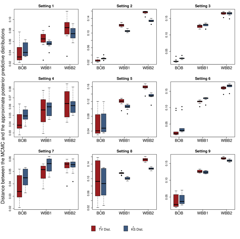
Figure 1: Boxplots of the $\hat{\text{TV}}$ and $\hat{\text{KS}}$ distances between the MCMC posterior predictive and the posterior predictive obtained by each one of the approximate methods based on ten independent runs per setting.

Table 2: Averages of the $\hat{\text{TV}}$ and $\hat{\text{KS}}$ distances between the MCMC posterior predictive and the posterior predictive obtained by each one of the approximate methods based on ten independent runs per setting.

Setting			1	2	3	4	5	6	7	8	9
$\hat{\text{TV}}$	BOB		0.042	0.025	0.021	0.042	0.057	0.035	0.037	0.092	0.038
			(0.007)	(0.001)	(0.002)	(0.003)	(0.010)	(0.010)	(0.003)	(0.016)	(0.006)
	WBB1		0.063	0.121	0.126	0.055	0.119	0.117	0.049	0.115	0.126
			(0.005)	(0.001)	(0.002)	(0.005)	(0.003)	(0.002)	(0.002)	(0.001)	(0.001)
	WBB2		0.084	0.156	0.165	0.063	0.158	0.159	0.054	0.152	0.165
			(0.007)	(0.002)	(0.002)	(0.005)	(0.003)	(0.002)	(0.002)	(0.002)	(0.001)
$\hat{\text{KS}}$	BOB		0.045	0.031	0.029	0.049	0.061	0.044	0.045	0.082	0.043
			(0.004)	(0.001)	(0.001)	(0.002)	(0.009)	(0.009)	(0.002)	(0.012)	(0.005)
	WBB1		0.058	0.106	0.129	0.059	0.105	0.127	0.055	0.100	0.124
			(0.004)	(0.001)	(0.002)	(0.003)	(0.002)	(0.002)	(0.002)	(0.001)	(0.001)
	WBB2		0.074	0.133	0.164	0.062	0.134	0.165	0.054	0.127	0.158
			(0.004)	(0.001)	(0.002)	(0.003)	(0.003)	(0.003)	(0.002)	(0.001)	(0.001)

NOTE: Standard errors are provided in parentheses. The best performance, across each setting, is presented in bold.

Moreover, we are also interested in analyzing the effect of the sample size on the different posterior approximations. Thus, Figure 2 presents the results of an additional experiment where we fix $d=10$ and $K=2$, and consider various sample sizes spanning from $n=25$ to $n=500$. More precisely, Figure 2 displays the $\hat{\text{TV}}$ and $\hat{\text{KS}}$ distances between the MCMC and the approximate posterior predictive distributions, as a function of $n$. We observe that, across all methods, the $\hat{\text{TV}}$ and $\hat{\text{KS}}$ distances decrease, as $n$ increases. This is consistent with the asymptotic properties from WBB and BOB. However, we can see that BOB persistently outperforms WBB, especially when $n$ is small. This illustrates the fact that under fixed sample sizes, BOB yields a better approximation to the Bayesian posterior. Asymptotically, though, we can observe that WBB and BOB converge to the same limiting distribution, which is desirable as WBB possesses appealing asymptotic properties. Altogether, we have that BOB is a reliable method for approximate posterior sampling, which can be applied in a wide range of problems with different dimensions and sample sizes.

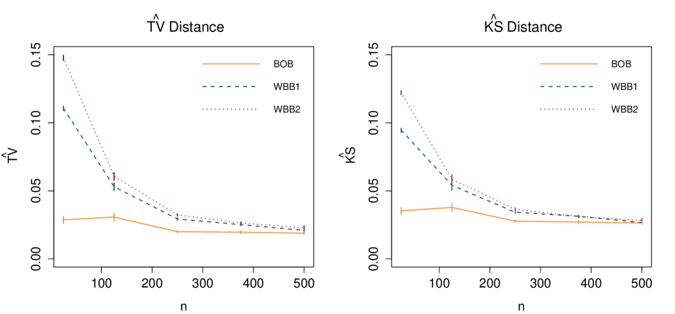
Figure 2: $\hat{\text{TV}}$ and $\hat{\text{KS}}$ distances between the MCMC and the approximate posterior predictive distributions as a function of $n$, with $d=10$ and $K=2$. The curves were produced by averaging across ten independent runs. Error bars indicate one standard error.

5 Analysis of Benchmark Data

To further demonstrate BOB’s performance and practical utility, we apply it to the widely analyzed wine data (Forina et al.,, 1986). The data consists of $d=27$ chemical properties for $n=178$ specimens belonging to $K=3$ types of wine, namely Barbera, Barolo, and Grignolino, produced in Italy’s Piedmont region. From the Barbera type we have 48 specimens, from Barolo we have 59 specimens, and from Grignolino we have 71 specimens. The idea is to cluster types of wine based on the chemical features of each specimen. A detailed description of the 27 features is presented in the supplementary materials. As preprocessing, we standardize the data so that each feature has mean 0 and variance 1. To set the prior hyperparameters, we follow the same approach as in section 4.1. Again, we obtain $S=2000$ posterior draws using BOB, WBB1 and WBB2. In the case of NUTS, we run the algorithm for 4000 iterations and discard the first half as a burn-in period. For BOB, we use a mini-batch of size $S_{b}=1000$ to construct $\hat{\mathcal{L}}(\boldsymbol{x})$.

Figure 3 shows the posterior and posterior predictive densities for selected variables from the wine data obtained via NUTS, BOB and WBB1. More precisely, row 1 presents the posterior KDEs of $(\mu_{\texttt{colour}},\mu_{\texttt{ODdw}})$, where colour is the colour intensity from each specimen and ODdw is the $OD_{280}/OD_{315}$ ratio of diluted wines. Row 2 presents the posterior predictive KDEs of $(y_{\text{new},\texttt{colour}},y_{\text{new},\texttt{ODdw}})$. We can observe a reasonable agreement between the three methods. NUTS, however, tends to shrink much more aggressively towards zero than BOB and WBB1. We can also observe that WBB1 induces the least shrinkage and tend to overestimate the posterior variances of $\boldsymbol{\mu}_{k}$ relative to NUTS. Interestingly, even if WBB1 overestimates the posterior variances of $\boldsymbol{\mu}_{k}$, it ends up underestimating the variances in the posterior predictive distribution, which suggests that WBB1 is not capturing well the posterior distribution of $\boldsymbol{\Sigma}_{k}$. Additional posterior density plots are provided in the supplementary materials, where we can observe similar patterns across different variables from the wine data. Moreover, in Table 3, we present the $\hat{\text{TV}}$ and $\hat{\text{KS}}$ distances between the MCMC and the approximate posterior predictive distributions. We can observe that BOB constantly returns the closest approximation to the MCMC posterior predictive, illustrating BOB’s reliable applicability in real-world problems.

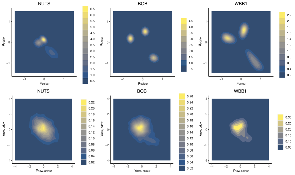
Figure 3: Posterior and post. predictive KDEs for selected variables from the wine data.

Table 3: $\hat{\text{TV}}$ and $\hat{\text{KS}}$ distances between the MCMC posterior predictive and the posterior predictive, for the wine data, obtained by each one of the approximate methods.

	BOB	WBB1	WBB2
$\hat{\text{TV}}$	0.037	0.075	0.100
$\hat{\text{KS}}$	0.042	0.071	0.089

NOTE: The best performance, across each metric, is presented in bold.

6 Discussion

In this article, we developed BOB, a novel computational methodology for approximate posterior sampling. We build on WLB and WBB ideas, which are based on the premise that optimizing randomly weighted posterior densities can be faster and less computationally intensive than sampling from an intractable posterior. BOB, however, tackles the problem of selecting the distribution of the random weights under arbitrary sample sizes, which has not been addressed before. This is automatically done by minimizing a black-box and noisy version of the reverse KL divergence between the Bayesian posterior and an approximate posterior induced by random weighting. We have demonstrated that, under fixed sample sizes, BOB outperforms competing approaches in recovering the Bayesian posterior while retaining key asymptotic properties from existing methods. Based on these results, we can conclude that BOB is a reliable approximate posterior sampler. On the whole, BOB joins a growing body of literature, which aims to draw practitioner’s attention toward posterior samplers beyond traditional MCMC algorithms (Nie and Ročková, 2023b, ; Newton et al.,, 2021). Thus, extending BOB (and BOB-like methodologies) from GMMs with conjugate priors to arbitrary posterior distributions presents an exciting research opportunity, which we leave for future work.

Supplementary Materials for “BOB: Bayesian Optimized Bootstrap with Applications to Gaussian Mixture Models”
Santiago Marin   Bronwyn Loong   Anton Westveld

S.1 Proof of Proposition 1

From (8), we have that the update of $\boldsymbol{\mu}_{k}$ and $\boldsymbol{\Sigma}_{k}$ is given by

$$\bigl{(}\boldsymbol{\mu}_{k}^{(t+1)},\boldsymbol{\Sigma}_{k}^{(t+1)}\bigr{)}=\operatorname*{arg\,max}_{\boldsymbol{\mu}_{k},\boldsymbol{\Sigma}_{k}}\bigl{\{}h(\boldsymbol{\mu}_{k},\boldsymbol{\Sigma}_{k})\bigr{\}},$$

with

$$\begin{split}h(\boldsymbol{\mu}_{k},\boldsymbol{\Sigma}_{k})&=-\frac{1}{2}\sum_{i=1}^{n}\left(u_{i}q_{ik}\left[\log|\boldsymbol{\Sigma}_{k}|+\left(\mathbf{y}_{i}-\boldsymbol{\mu}_{k}\right)^{\prime}\boldsymbol{\Sigma}_{k}^{-1}\left(\mathbf{y}_{i}-\boldsymbol{\mu}_{k}\right)\right]\right)-\frac{\tilde{u}_{\Sigma_{k}}\operatorname{tr}(\boldsymbol{\Psi}_{k}\boldsymbol{\Sigma}_{k}^{-1})}{2}\\ &\quad-\frac{\tilde{u}_{\mu_{k}}\lambda_{k}}{2}(\boldsymbol{\mu}_{k}-\boldsymbol{\beta}_{k})^{\prime}\boldsymbol{\Sigma}_{k}^{-1}(\boldsymbol{\mu}_{k}-\boldsymbol{\beta}_{k})-\tilde{u}_{\Sigma_{k}}\left(\frac{\nu_{k}+d}{2}+1\right)\log|\boldsymbol{\Sigma}_{k}|\\ &\overset{(*)}{=}-\frac{\tilde{n}_{k}}{2}\log|\boldsymbol{\Sigma}_{k}|-\frac{1}{2}\operatorname{tr}\left[\left(\tilde{n}_{k}(\tilde{\bar{\mathbf{y}}}_{k}-\boldsymbol{\mu}_{k})(\tilde{\bar{\mathbf{y}}}_{k}-\boldsymbol{\mu}_{k})^{\prime}+\tilde{\mathbf{S}}_{k}\right)\boldsymbol{\Sigma}_{k}^{-1}\right]\\ &\quad-\left(\frac{\tilde{\nu}_{k}+d}{2}+1\right)\log|\boldsymbol{\Sigma}_{k}|-\frac{1}{2}\operatorname{tr}\left(\tilde{\boldsymbol{\Psi}}_{k}\boldsymbol{\Sigma}_{k}^{-1}\right)-\frac{\tilde{\lambda}_{k}}{2}\operatorname{tr}\left[(\boldsymbol{\mu}_{k}-\boldsymbol{\beta}_{k})(\boldsymbol{\mu}_{k}-\boldsymbol{\beta}_{k})^{\prime}\boldsymbol{\Sigma}_{k}^{-1}\right]\\ &=-\left(\frac{\bar{\nu}_{k}+d}{2}+1\right)\log|\boldsymbol{\Sigma}_{k}|-\frac{1}{2}\operatorname{tr}\left(\bar{\boldsymbol{\Psi}}_{k}\boldsymbol{\Sigma}_{k}^{-1}\right)-\frac{\bar{\lambda}_{k}}{2}(\boldsymbol{\mu}_{k}-\bar{\boldsymbol{\beta}}_{k})^{\prime}\boldsymbol{\Sigma}_{k}^{-1}(\boldsymbol{\mu}_{k}-\bar{\boldsymbol{\beta}}_{k}),\end{split}$$

where $(*)$ follows from the fact that $\sum_{i=1}^{n}\mathbf{b}_{i}^{\prime}\mathbf{A}\mathbf{b}_{i}=\operatorname{tr}(\mathbf{B}^{\prime}\mathbf{BA})$, where $\mathbf{B}\in\mathbb{R}^{n\times d}$ denotes the matrix whose $i$-th row is $\mathbf{b}_{i}^{\prime}\in\mathbb{R}^{1\times d}$, and by writing $(\mathbf{y}_{i}-\boldsymbol{\mu}_{k})$ as $(\mathbf{y}_{i}-\tilde{\bar{\mathbf{y}}}_{k}+\tilde{\bar{\mathbf{y}}}_{k}-\boldsymbol{\mu}_{k})$. ∎

S.2 Additional Posterior Density Plots

Figures 4 and 5 present posterior density plots for $(\texttt{alcohol},\texttt{ODdw})$ and $(\texttt{alcohol},\texttt{colour})$, respectively. We observe that NUTS shrinks much more aggressively towards zero. We can also observe that WBB1 induces the least shrinkage and tend to overestimate posterior variances relative to NUTS. Interestingly, it might look like NUTS is getting stuck in a local mode, failing to explore the entire posterior distribution. WBB and BOB, on the other hand, clearly recover the multimodality of the Gaussian Mixture.

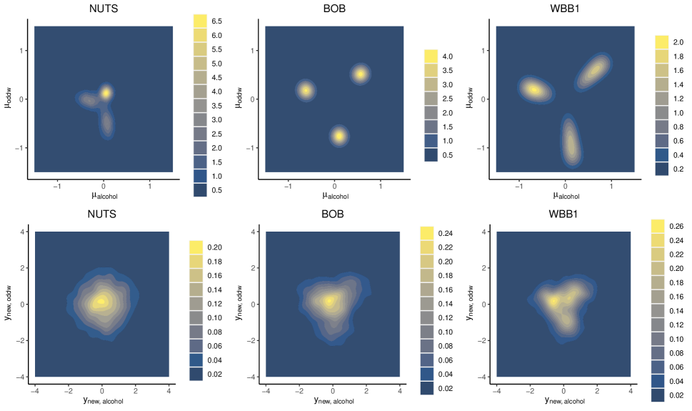
Figure 4: Posterior density plots for $(\texttt{alcohol},\texttt{ODdw})$

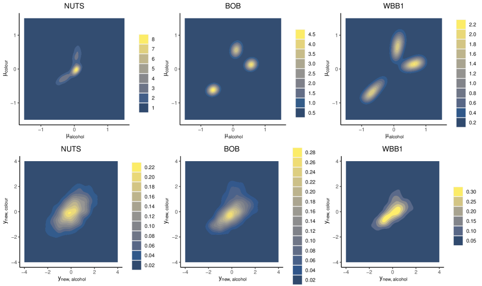
Figure 5: Posterior density plots for $(\texttt{alcohol},\texttt{colour})$

S.3 Features in the Wine data

List of 27 chemical features in the Wine data:

1. alco: Alcohol percentage

2. sug: Sugar-free extract

3. acid: Fixed acidity

4. tart: Tartaric acid

5. mal: Malic acid

6. uro: Uronic acid

7. pH: pH

8. ash: Ash

9. akash: Alkalinity of ash

10. pot: Potassium

11. cal: Calcium

12. mag: Magnesium

13. phos: Phosphate

14. chl: Chloride

15. phen: Total phenols

16. flav: Flavanoids

17. nflav: Nonflavanoid phenols

18. proa: Proanthocyanins

19. col: Colour intensity

20. hue: Hue

21. ODdw: $OD_{280}/OD_{315}$ of diluted wines

22. ODfl: $OD_{280}/OD_{315}$ of flavanoids

23. gly: Glycerol

24. buta: 2,3-butanediol

25. nit: Total nitrogen

26. prol: Proline

27. met: Methanol

References

- Allassonnière and Chevallier, (2021) Allassonnière, S. and Chevallier, J. (2021). A new class of stochastic em algorithms. escaping local maxima and handling intractable sampling. Computational Statistics & Data Analysis, 159:107159.
- Bishop, (2006) Bishop, C. M. (2006). Pattern recognition and machine learning. Springer New York, NY.
- Blei et al., (2017) Blei, D. M., Kucukelbir, A., and McAuliffe, J. D. (2017). Variational inference: A review for statisticians. Journal of the American Statistical Association, 112(518):859–877.
- Bull, (2011) Bull, A. D. (2011). Convergence rates of efficient global optimization algorithms. Journal of Machine Learning Research, 12(10).
- Carpenter et al., (2017) Carpenter, B., Gelman, A., Hoffman, M. D., Lee, D., Goodrich, B., Betancourt, M., Brubaker, M. A., Guo, J., Li, P., and Riddell, A. (2017). Stan: A probabilistic programming language. Journal of Statistical Software, 76.
- Celeux et al., (2000) Celeux, G., Hurn, M., and Robert, C. P. (2000). Computational and inferential difficulties with mixture posterior distributions. Journal of the American Statistical Association, 95(451):957–970.
- Dempster et al., (1977) Dempster, A. P., Laird, N. M., and Rubin, D. B. (1977). Maximum likelihood from incomplete data via the em algorithm. Journal of the Royal Statistical Society Series B: Statistical Methodology, 39(1):1–22.
- Diebolt and Robert, (1994) Diebolt, J. and Robert, C. P. (1994). Estimation of finite mixture distributions through bayesian sampling. Journal of the Royal Statistical Society Series B: Statistical Methodology, 56(2):363–375.
- Fong et al., (2019) Fong, E., Lyddon, S., and Holmes, C. (2019). Scalable nonparametric sampling from multimodal posteriors with the posterior bootstrap. International Conference on Machine Learning, pages 1952–1962.
- Forina et al., (1986) Forina, M., Armanino, C., Castino, M., and Ubigli, M. (1986). Multivariate data analysis as a discriminating method of the origin of wines. Vitis, 25:189–201.
- Fraley and Raftery, (2002) Fraley, C. and Raftery, A. E. (2002). Model-based clustering, discriminant analysis, and density estimation. Journal of the American Statistical Association, 97(458):611–631.
- Friedman et al., (2008) Friedman, J., Hastie, T., and Tibshirani, R. (2008). Sparse inverse covariance estimation with the graphical lasso. Biostatistics, 9(3):432–441.
- Gelman et al., (2014) Gelman, A., Carlin, J. B., Stern, H. S., Dunson, D. B., Vehtari, A., and Rubin, D. B. (2014). Bayesian Data Analysis, 3rd edn. CRC Press, Boca Raton, FL.
- Gelman and Rubin, (1992) Gelman, A. and Rubin, D. B. (1992). Inference from iterative simulation using multiple sequences. Statistical Science, 7(4):457–472.
- Giordano et al., (2023) Giordano, R., Ingram, M., and Broderick, T. (2023). Black box variational inference with a deterministic objective: Faster, more accurate, and even more black box. arXiv preprint arXiv:2304.05527.
- Grazian, (2023) Grazian, C. (2023). A review on bayesian model-based clustering. arXiv preprint arXiv:2303.17182.
- Hoffman and Gelman, (2014) Hoffman, M. D. and Gelman, A. (2014). The no-u-turn sampler: Adaptively setting path lengths in hamiltonian monte carlo. Journal of Machine Learning Research, 15(47):1593–1623.
- Izenman and Sommer, (1988) Izenman, A. J. and Sommer, C. J. (1988). Philatelic mixtures and multimodal densities. Journal of the American Statistical Association, 83(404):941–953.
- Jones, (2001) Jones, D. R. (2001). A taxonomy of global optimization methods based on response surfaces. Journal of Global Optimization, 21:345–383.
- Jones et al., (1998) Jones, D. R., Schonlau, M., and Welch, W. J. (1998). Efficient global optimization of expensive black-box functions. Journal of Global Optimization, 13:455–492.
- Kandasamy et al., (2020) Kandasamy, K., Vysyaraju, K. R., Neiswanger, W., Paria, B., Collins, C. R., Schneider, J., Poczos, B., and Xing, E. P. (2020). Tuning hyperparameters without grad students: Scalable and robust bayesian optimisation with dragonfly. Journal of Machine Learning Research, 21(81):1–27.
- Kim et al., (2015) Kim, S., Pasupathy, R., and Henderson, S. G. (2015). A guide to sample average approximation. Handbook of simulation optimization, pages 207–243.
- Kirkpatrick et al., (1983) Kirkpatrick, S., Gelatt Jr, C. D., and Vecchi, M. P. (1983). Optimization by simulated annealing. Science, 220(4598):671–680.
- Lartigue et al., (2022) Lartigue, T., Durrleman, S., and Allassonnière, S. (2022). Deterministic approximate em algorithm; application to the riemann approximation em and the tempered em. Algorithms, 15(3):78.
- Littell et al., (2000) Littell, R. C., Pendergast, J., and Natarajan, R. (2000). Modelling covariance structure in the analysis of repeated measures data. Statistics in Medicine, 19(13):1793–1819.
- Lyddon et al., (2019) Lyddon, S. P., Holmes, C., and Walker, S. (2019). General bayesian updating and the loss-likelihood bootstrap. Biometrika, 106(2):465–478.
- Martinez-Cantin, (2014) Martinez-Cantin, R. (2014). Bayesopt: A bayesian optimization library for nonlinear optimization, experimental design and bandits. Journal of Machine Learning Research, 15(115):3915–3919.
- Nemirovski et al., (2009) Nemirovski, A., Juditsky, A., Lan, G., and Shapiro, A. (2009). Robust stochastic approximation approach to stochastic programming. SIAM Journal on Optimization, 19(4):1574–1609.
- Newton, (1991) Newton, M. A. (1991). The weighted likelihood bootstrap and an algorithm for prepivoting. PhD dissertation, Department of Statistics, University of Washington, Seattle, WA.
- Newton et al., (2021) Newton, M. A., Polson, N. G., and Xu, J. (2021). Weighted bayesian bootstrap for scalable posterior distributions. Canadian Journal of Statistics, 49(2):421–437.
- Newton and Raftery, (1994) Newton, M. A. and Raftery, A. E. (1994). Approximate bayesian inference with the weighted likelihood bootstrap. Journal of the Royal Statistical Society Series B: Statistical Methodology, 56(1):3–48.
- Ng and Newton, (2022) Ng, T. L. and Newton, M. A. (2022). Random weighting in lasso regression. Electronic Journal of Statistics, 16(1):3430–3481.
- Ni et al., (2020) Ni, Y., Müller, P., Diesendruck, M., Williamson, S., Zhu, Y., and Ji, Y. (2020). Scalable bayesian nonparametric clustering and classification. Journal of Computational and Graphical Statistics, 29(1):53–65.
- (34) Nie, L. and Ročková, V. (2023a). Bayesian bootstrap spike-and-slab lasso. Journal of the American Statistical Association, 118(543):2013–2028.
- (35) Nie, L. and Ročková, V. (2023b). Deep bootstrap for bayesian inference. Philosophical Transactions of the Royal Society A, 381(2247):20220154.
- Omori et al., (2007) Omori, Y., Chib, S., Shephard, N., and Nakajima, J. (2007). Stochastic volatility with leverage: Fast and efficient likelihood inference. Journal of Econometrics, 140(2):425–449.
- Pompe, (2021) Pompe, E. (2021). Introducing prior information in weighted likelihood bootstrap with applications to model misspecification. arXiv preprint arXiv:2103.14445.
- Rasmussen and Williams, (2005) Rasmussen, C. E. and Williams, C. K. I. (2005). Gaussian Processes for Machine Learning. The MIT Press.
- Raymaekers and Zamar, (2022) Raymaekers, J. and Zamar, R. H. (2022). Regularized k-means through hard-thresholding. Journal of Machine Learning Research, 23(93):1–48.
- Sambridge, (2014) Sambridge, M. (2014). A Parallel Tempering algorithm for probabilistic sampling and multimodal optimization. Geophysical Journal International, 196(1):357–374.
- Schilling, (2017) Schilling, R. L. (2017). Measures, integrals and martingales. Cambridge University Press.
- Snoek et al., (2012) Snoek, J., Larochelle, H., and Adams, R. P. (2012). Practical bayesian optimization of machine learning algorithms. Advances in Neural Information Processing Systems, 25.
- Stephens, (2000) Stephens, M. (2000). Dealing with label switching in mixture models. Journal of the Royal Statistical Society Series B: Statistical Methodology, 62(4):795–809.
- Stringer et al., (2023) Stringer, A., Brown, P., and Stafford, J. (2023). Fast, scalable approximations to posterior distributions in extended latent gaussian models. Journal of Computational and Graphical Statistics, 32(1):84–98.
- Sun et al., (2012) Sun, W., Wang, J., and Fang, Y. (2012). Regularized k-means clustering of high-dimensional data and its asymptotic consistency. Electronic Journal of Statistics, 6:148–167.
- Van Havre et al., (2015) Van Havre, Z., White, N., Rousseau, J., and Mengersen, K. (2015). Overfitting bayesian mixture models with an unknown number of components. PloS one, 10(7):e0131739.
- Wade and Ghahramani, (2018) Wade, S. and Ghahramani, Z. (2018). Bayesian Cluster Analysis: Point Estimation and Credible Balls (with Discussion). Bayesian Analysis, 13(2):559 – 626.